semartcam scheduler: semantics driven real-time data collection

SPECIAL ISSUE

SEMARTCam scheduler: semantics driven real-time datacollection from indoor camera networks to maximize eventdetection

Ronen Vaisenberg • Sharad Mehrotra •

Deva Ramanan

Received: 30 June 2009 / Accepted: 14 December 2009

� Springer-Verlag 2010

Abstract A distributed camera network allows for many

compelling applications such as large-scale tracking or

event detection. In most practical systems, resources are

constrained. Although one would like to probe every

camera at every time instant and store every frame, this is

simply not feasible. Constraints arise from network band-

width restrictions, I/O and disk usage from writing images,

and CPU usage needed to extract features from the images.

Assume that, due to resource constraints, only a subset of

sensors can be probed at any given time unit. This paper

examines the problem of selecting the ‘‘best’’ subset of

sensors to probe under some user-specified objective—e.g.,

detecting as much motion as possible. With this objective,

we would like to probe a camera when we expect motion,

but would not like to waste resources on a non-active

camera. The main idea behind our approach is the use of

sensor semantics to guide the scheduling of resources.

We learn a dynamic probabilistic model of motion corre-

lations between cameras, and use the model to guide

resource allocation for our sensor network. Although pre-

vious work has leveraged probabilistic models for sensor-

scheduling, our work is distinct in its focus on real-time

building-monitoring using a camera network. We validate

our approach on a sensor network of a dozen cameras

spread throughout a university building, recording mea-

surements of unscripted human activity over a two week

period. We automatically learnt a semantic model of

typical behaviors, and show that one can significantly

improve efficiency of resource allocation by exploiting this

model.

Keywords Video surveillance � Algorithms �Sensor network � Real-time

1 Introduction

Consider a camera-based surveillance system deployed

throughout a building environment. The task of the system

is to process a typically immense quantity of data in real-

time, possibly forwarding ‘‘suspicious’’ activities to a

human for further inspection. We envision that multiple

components are involved in this processing: low-level

motion detection algorithms will identify specific regions

and cameras of interest, camera sensors must record and

transmit images to a central server, and finally, high-level

object and activity recognition algorithms should identify

suspicious movement patterns that are finally presented to

human user. A vital aspect of this processing is that it must

be done in real time.

Real-time restrictions are particularly limiting because

of the enormous computational demands and the resource

limitations imposed by a large-scale network. CPU

resources limit the number of frames we can process, and

image file sizes limit the amount of images that can be

transmitted throughout a network. In this work, we con-

sider a fundamental resource limitation due to network

bandwidth: we can only probe K out of N cameras at each

time instant, where K B N. Under such restrictions, we

examine: what is the system’s optimal plan of sensor

probes?

R. Vaisenberg (&) � S. Mehrotra � D. Ramanan

School of Information and Computer Sciences,

University of California, Irvine, CA 92697-3425, USA

e-mail: [email protected]

S. Mehrotra


D. Ramanan


123

J Real-Time Image Proc

DOI 10.1007/s11554-009-0147-8

Our intuition is that much of the behavior and activity in

a building, even for the ‘‘suspicious’’ cases, follows certain

low-level semantics—people enter and exit through doors,

walk along hallways, wait in front of elevators, etc. We

demonstrate that one can build a semantic model of such

behavior, and use the model to guide efficient resource

allocation for the K available sensor probes.

We look at the planning problem as a sub-task selection

problem. The sub-tasks were selected to optimize an

application-dependant benefit function (BF). For example,

a particular application may want all image frames for

which there is motion (all motion events are equally

important), while another application may define that two

images of two different individuals are more important

than two of the same person.

Another consideration is the cost of a plan, in terms of

network resources, referred to as cost function (CF). Dif-

ferent plans may not cost the same in terms of network

resources since it may be less expensive to probe the same

sensor at the next time instant. In a fully general model,

one might also place the number of sensor probes K into

the cost function.

A major motivating application for such an algorithm is

a real-time display of image data collected from a network

cameras. As the number of cameras is much larger than the

number of available screens for display, a subset of the

camera feeds need to be selected at any time point based on

a user defined, benefit function, e.g., visualize as many

motion events in the camera network on a display of k

screens. Currently, most such surveillance systems follow a

Round-Robin approach to schedule the camera feeds to

display on the available screens.

Formally, we define a plan for N cameras to be a binary

vector of length N that specifies which cameras will be

probed in the next time instant. Plan = {Ci|1 B i B N},

where Ci [ {0, 1}.

Our task is not only to know when and where motion

was detected but also to probe the cameras for frames for a

surveillance application or a human operator. Motion is an

underlying primitive, that is used to select data that might

contain interesting events.

To illustrate how the choice of sub-tasks affects a real-

time tracking system, consider the following example.

Suppose we have N = 6 cameras and budget of K = 1

probes per time instant. At time t, a frame processed from

camera cj reveals motion. Semantic correlation data col-

lected off-line suggests that motion is expected to continue

at cj at probability pstay(cj). Suppose further that at time t-3,

motion was detected at camera ck. Semantic correlation data

further suggests that given the motion was seen at ck at t-3,

motion is expected to be seen at camera ccorrelated to k with

probability p correlationðck; ccorrelated to k; 3Þ. This proba-

bility is a function of the time elapsed and the two cameras in

order: from, to. At the same time, the semantic information

suggests that motion can start spontaneously at cspont with

probability pspont(cspont).

These probabilities provide estimates as to where

motion is expected (we will see how they can be computed

shortly). The actual sub-task selection should be performed

based on the specific benefit/cost functions defined. Note

that decisions are made based on partial knowledge of

where motion is since we only know what we have ‘‘seen’’.

Related work is discussed in detail in Sect. 2, for the

completeness of presentation, we briefly describe related

work and its relation to ours.

Scheduling under resource constraints for data collection

has been previously studied in a variety of contexts [8, 21];

e.g., Markov decision processes, in sensor networks to create

an accurate system state representation or for optimizing

query performance [6, 7, 22]. Such work has also exploited

semantics of the environment and/or phenomena being

sensed to optimize resources (e.g., powering down sensors

and/or reducing the rate at which they transmit). While such

previous work is very related to our approach, none of the

related strategies applies directly to our real-time camera

network setting, as there are several aspects of our work that

make it unique. First, we study resource constrained

scheduling in the setting where sensors are video cameras

which, to the best of our knowledge, has not been studied

previously. The nature of cameras and activity these cam-

eras capture provide new opportunities for optimization—

e.g., exploiting cross correlation of motion amongst cameras

to predict future motion. Second, our goal is to design a

principled extensible framework that enables diverse

semantics to be incorporated in making scheduling deci-

sions—we illustrate the framework using three semantic

concepts (all learnt from data): a priori probability, self-

correlation, and cross-correlation. Finally, we illustrate the

utility of the technique on real data captured using video

cameras deployed at different locations of the building. We

believe that the sub-task selection problem is a central, and

frequent, one in multimedia applications [14].

Generally, there is a limit on how many processing tasks

can be applied in real-time and an optimal subset of the

computation tasks to be selected. In most of these cases,

semantic information seems to be a promising way to

efficiently direct the available resources.

In order to study the sub-task selection problem, we

made several assumptions:

• Semantics available are only of those of motion.

Although more information can potentially be extracted

as semantic information, we focused only on motion.

• Semantic system information is learned off-line with no

budget constraints and is not updated while in

operation.


123

• Prediction window is t = 1. Although, it may be

important to plan for the next t seconds1 extending our

approach to support this is part of our planned work for

the future, and for this work we assume that t = 1.

• Homogeneity assumption. In order to simplify the

algorithms, we assumed that the cameras are homoge-

nous in terms of probe costs. As such, the cost function

was always constant. We are leaving the study of the

effects of incorporating cost functions to future work.

• Scheduling Decisions are made by a (logically2) central

node which knows the current state of the system and

its history.

Push versus Pull Note that our approach is based on a

pull-based model wherein data is probed from cameras

based on a schedule generated by exploiting semantics. An

alternate approach could be for cameras to push data

whenever an event of interest is observed (push-based

model). While push-based models are interesting, they

display a few shortcomings in our setting. First, push-based

models depend upon cameras to have some computational

resources (which is not the case in our infrastructure).

Second, such models require basic event detection to be

done at the camera which is achievable if events are well

defined but more complex in settings such as surveillance

where the interest may be in ill-defined events such as

‘‘abnormal’’ event. Of course, push-models could be based

simply on motion detection but then scalability becomes an

issue since, depending the usage of the monitored space,

multiple cameras may detect motion together leading to

network resource saturation. Even in our experimental set

up, push based model (which we used for collecting

training data) led to significant delays (about 30 s in some

cases). This is specially the case during periods of high

activity (e.g., in-between classes) when all sensors are

likely to have motion. The delay caused due to network

resources adversely affects the real-time nature of the

application. Finally, push-based approach at the motion

level is not as robust as the pull-based model we use since

false positives such as lighting changes from doors

swinging, etc. would result in data transmission. In this

paper, we concentrate on exploiting semantics in a pull-

based approach—a hybrid strategy based on combining

both push and pull offers an interesting direction for future

research.

As we proceed, we will address the following questions:

1. What are the options in selecting sub-tasks?

2. What kind of semantic information needs to be

collected off-line, for the case of motion?

3. Which approach proves to work better on real-data?

4. What are the underlying reasons for the observed

differences of sub-task selection strategies?

The rest of the paper is organized as follows: in

Sect. 2, we discuss related work. Section 3 describes our

system architecture and the semantics exploited in our

framework. In Sect. 4, we introduce the models that we

used to learn the semantics. Section 5 discusses different

strategies for sub-task selection. Section 6 describes our

implementation of the framework and presents accompa-

nying results. We conclude and discuss future work in

Sect. 7.

2 Related work

This work is an extended version of [20]. The three main

contributions in this work are:

• We extend the semantic model to include semantics of

event start and event ongoing and create a new model

that out performs the previous—motion only semantic

model. This shows how other types of semantics can be

added to the model, and used to improve the perfor-

mance of the scheduler.

• We give a detailed description of the two implemen-

tation pitfalls we identified: probe based on sampling,

as opposed to probing based on the order of probabil-

ities (high to low) and predict only based on motion that

was probed. The importance of avoiding these pitfalls is

illustrated by an experiment that shows a significant

improvement in the recall of events.

• We evaluate the scheduling algorithm based on other

benefit functions, such as event start, number of

different events and average delay between the event

start and the first second it is probed.

To the best of our knowledge, we are first to address

the problem of scheduling access in a camera network

using a semantic model of building activities. Our

correlation-based model is simple enough to be imple-

mented in real-time, yet powerful enough to capture

meaningful semantics of typical behavior. However, there

is numerous relevant and related work which we now

discuss.

The general problem we addressed relates to the prob-

lem of deadline assignment to different jobs [9] where a

global task is to be completed before a deadline and mul-

tiple processing components are available for processing.

We can think of the task of event capture as a global task

which is to be detected until a deadline, the end of the

event. Our work mainly as the question we try to answer is

which nodes should take part in the processing when

1 For example, due to network delays, deployment has to be done in

advance.2 More on this in Sect. 7.


123

different node have different cost/benefit related to the task

in hand. Only a specific node (the one where the event is in

the FOV) can help the system meet the ‘‘deadline’’ or in

our terminology, maximize event capture we exploit

semantics of motion to guide the selection of nodes to

probe, by definition nodes are not equivalent processing

units.

In the context of multimedia applications, [14] suggest a

scheduler for multimedia applications which supports

applications with time constraints. It adjusts the allocation

of resources dynamically and automatically shed real-time

tasks and regulate their execution rates when the system is

overloaded. This approach is similar in its motivation to

our work, however, we exploiting semantics for the

scheduling of data collection tasks.

In the context of video surveillance, [1] propose a new

approach known as experimental sampling which carries

out analysis on the environment and selects data of interest

while discarding the irrelevant data. In the case of multiple

surveillance cameras, the paper assumes that all video

frames are can be collected for processing at any given

time. The motivation is similar as out of the set of available

images, the most important ones need to be selected.

However, our problem is fundamentally different as we

address the problem given a resource limitation which

prevents the system from accessing all video frames.

In the context of sensor networks, [22] and [6] describe

a prediction based approach used to utilize battery con-

sumption in sensor networks. Only when the observed

value deviates from the expected value based on the pre-

diction model, by a pre-defined error bound, the sensor

transmits the observed value to the server. The error bound

is defined by the application according to different quality

requirements across sensors. [11] proposed an online

algorithm for creating approximation of a real valued time

series generated by wireless sensors, that guarantees that

the compressed representation satisfies a bound on the L?

distance. The compressed representation is used to reduce

the communication between the sensor and the server in a

sensor network.

In the domain of people and object tracking [17] and [4]

address the problem of tracking when the estimates of

location are not accurate, i.e., some of the generated esti-

mates are erroneous due to the inaccuracy of the capturing

sensor. The task in both papers was to reconstruct the

actual trajectory of the object being tracked with statistical

models, such as Kalman filters by [2] are utilized to find the

most probable trajectory. The kinds of problems that these

statistical models are used for try to estimate the location of

moving objects, for example tracking planes given a

wandering blip that appears every 10 seconds. Work by

Song et al. used semantic information to address the

problem of inaccuracy feature based tracking algorithms

that try to associate subjects seen at different cameras by

[19]. Here, the challenge is again individual tracking and

specifically, being able to associate two images from two

different cameras to the same person.

There is a large body of work on schedule optimization

within the sensor modeling literature, see [5, 8, 10, 21]. A

common approach is to build a probabilistic model of

object state and probe sensors that reduce the entropy, or

uncertainly in state, at the next time frame. Our application

is different in that, rather than reducing the uncertainty in

building state, we want to collect images of events (even if,

and indeed especially if, we are certain of their occurrence)

for further high-level processing. Directly modeling object

state is difficult in our scenario because a large number of

people move, interact, and enter/exit, making data associ-

ation and tracking extremely challenging. We take a dif-

ferent approach and directly model the environment itself

using a simple, but effective, sensor-correlation model.

Modeling people activity was studied by [8]. It was

found that a Poison process provided a robust and accurate

model for human behavior, such as people and car count-

ing, and showed that normal behavior can be separated

from unusual event behavior. In the context of intrusion

detection, [18] proposed a Markov modulated nonhomo-

geneous Poisson process model for telephone fraud

detection. Scott used only event time data, but detectors

based on Scott’s model may be combined with other

intrusion detection algorithms to accumulate evidence of

intrusion across continuous time. Our work differs as we

tried to find event of interest on real time under constraints.

One common task in sensor networks is topology

reconstruction—[12] explicitly do this in the context of

non-overlapping cameras. Our correlation model implicitly

not only encodes such a spatial topology, but also captures

temporal dependencies between sensors (Fig. 1c). We

know of no previous work on spatio-temporal structure

estimation, though we found it vital in our building envi-

ronment model.

3 Our approach

To study the sub-task selection problem, we postulate a

simple model where nodes are cameras and task is to pull

frames from nodes (cameras) such that an application

defined criteria, such as detect as much motion is maxi-

mized. A central server process (following the pull based

approach) decides which subset of frames to be analyzed

for each time unit3.

To address the scheduling problem, the approach we

adopt is to exploit semantics. While the framework we

3 We chose second, but other scales were possible to discrete time.


123

develop (which is based on probabilistic reasoning) is gen-

eral and can accommodate any type of semantics, we focus

on three different semantic concepts with which to illustrate

and experiment. We then show how the system can be

extended to accommodate other types of semantics as well.

The semantics of interest included:

1. A priori knowledge of where motion is likely to be.

Such semantics can be learned from the data by simply

detecting which camera is more likely to have an event

occurring. In the case of the building, it is likely that

the camera at the front door will see more motion than

other cameras. In addition, cameras in front of

classrooms (or meeting facilities) are likely to observe

events more often than others.

2. Self correlation of camera stream over time. Given that

a camera observes an event and given the camera’s

field of view (FOV), one could predict the probability

that the event will continue. Of course, this is a camera

specific property since it depends upon FOV as well as

how individuals in the FOV use the space. For

instance, a camera focussing on a long corridor will

have a person in view for a longer period of time

compared to a camera that is focused on an exit door.

3. Cross correlations between cameras. Clearly a person

who exits a FOV of one camera will be captured by

another depending upon the trajectory of the individual

and the placement of the cameras. Given that a person

exits the FOV of camera A, there is an implied

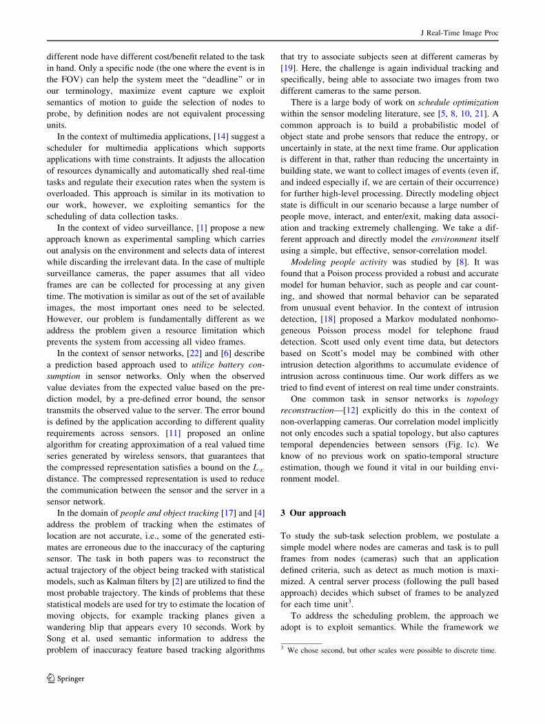
0 10 20 30 40 50 600

0.1

0.2

0.3

0.4

0.5

0.6

0.7

seconds

Pro

b of

mot

ion

Motion conditioned on cam2

cam1, floor2cam2, floor2cam3, floor2cam4, floor2cam5, floor4

0 10 20 30 40 50 600

0.05

0.1

0.15

0.2

0.25

0.3

0.35

0.4

seconds

Pro

b of

mot

ion

Motion conditioned on cam1

cam1, floor2cam2, floor2cam3, floor2cam4, floor2cam5, floor4

0 10 20 30 40 500

10

20

30

40

50

60

70

Number of Motion Events in All Sensors Over the Last 15 seconds

% F

rom

Tot

al

(a) (b)

(c) (d)

Fig. 1 Physical instrumentation and visualization of motion semantics. a Second floor, b cross-correlated, c only self correlated, d motion is

sparse over time


123

probability that he/she will enter into the FOV of

camera B.

Given the above, our approach to scheduling is as

follows:

1. We learn the above semantics from data.

2. We develop a framework, where given the state of the

system currently, we project the state in the near future

by determining probabilities of event (motion in FOV).

These probabilities are based on all the three semantic

concepts above. The three main modules of our

framework are:

• Task processing module Takes as an input a set of

cameras to probe (query plan) performs the que-

rying of the frames from the cameras and returns a

list of cameras where motion was detected.

• System semantics module Uses a pre-generated log,

containing list of cameras and time at which

motion was detected at each camera and outputs

semantic information in a form of correlation

matrix which is used by the scheduler.

• Scheduling module Uses the current state of the

system, i.e., the cameras at which motion was

detected, semantic information, BF Benefit Func-

tion, CF Cost Function and k Constraint on the

number of sensors to probe and returns a list of k

cameras to query (a query plan) which maximizes

BF and minimizes CF.

The semantic module computes the probabilities of the

following three events predicted to occur in the future:

(a) E(a priori(i)) motion starts at sensor i.

(b) E(Self-correlation(i, p)) motion continues at sensor i,

given that there was motion with probability p, at the

previous time unit.

(c) E(Cross-correlation(i, M)) motion at sensor i, given

M—a matrix containing the probability of motion for

all sensors for the last t time units.

Based on the probabilities of the above events, given

by the semantic module and the current state of the

system, detected by the task processing module the

scheduling module generates a schedule for the next time

unit under the constraints, that minimizes CF and max-

imizes BF.

We observe that this probabilistic framework is very

general. If we had some other semantics we could further

incorporate it as long as we can map the semantics to a

conditional probability between events over time.

Later on, we will offer other examples of semantics

which may be useful. The key technical challenge and

contributions of this paper were as follows:

1. Techniques to learn probabilities from past (as well as

current) data.

2. Techniques to schedule based on probabilities. The

key issue here is efficiency of computing the schedule

without a complex probabilistic analysis.

The next section describes our learning algorithms and

the scheduling algorithm followed by an experimental

setup, testing and validation.

4 Learning algorithms

The following sections describe the models that we con-

structed in order to capture semantics of motion. All of the

semantics extracted were learned from training data (see

Sect. 6 for information about how the data was collected).

In the following sections, subscript will denote time while

super script will denote camera.

4.1 A priori

Arguably, the simplest level of semantics exploits the fact

that certain cameras are more likely to see motion, and so

they should be probed more often. We compute the prob-

ability of seeing motion at a camera from training data as

follows: we divide the number of time instants where

motion was observed by the total time period.

4.2 Self-correlation

Assume the state of a camera at time t is st [ {0, 1},

signifying a motion event or the lack thereof. Let us call the

observed motion reading from a camera at time t as ot

[ {0, 1}. We assume a Hidden Markov Model (HMM) [16]

of the state and observations

Pðo; sÞ ¼ PðojsÞPðsÞ ð1Þ

Pðo; sÞ ¼ Pðs1ÞY

t [ 1

PðotjstÞPðstjst�1Þ ð2Þ

The parameters of the HMM are (SC, B, p) where

SC ¼ Pðstjst�1Þ ¼a 1� a

1� b b

� �ð3Þ

B ¼ PðotjstÞ ¼1 0

0 1

� �ð4Þ

p ¼ PðsoÞ ¼ p1 p2½ �T ð5Þ

For simplicity, we use a zero-noise observation model

(Eq. 2), though we could learn these values as well. Here,

a = P(st = 0|st-1 = 0) and b = P(st = 1|st-1 = 1).

Inference (computing P(st)) Exact inference in an HMM

can be performed with the forward–backward algorithm [16].


123

Since we are concerned only with the current state for online

scheduling, we need only to implement the forward stage.

This can be implemented with a prediction step that predicts

P(st) from P(st-1) using the dynamic model A, and a correction

step that refines P(st) using the observations ot (and B) if

available.

Learning (estimating SC, B, p) One can learn model

parameters from noisy data using the Expectation Maxi-

mization algorithm [16]. Since our observation model is

noise-free, we can learn model parameters directly by

frequency estimation. For example, b from Eq. 3 is set to

the fraction of times one observed motion in a camera

given there was motion in the previous second (from

training data).

4.3 Cross-sensor correlation

We would like to capture the intuition that, given that

motion is observed in a particular camera, the scheduler

should probe other cameras that lie on typical walking

paths emanating from that camera. An important consid-

eration is that it can take many time units, to move between

cameras in a typical network. Hence a first-order Markov

model no longer applies.

For ease of exposition, we first describe a first-order

multi-sensor model, but will extend it subsequently to a

Mth order model that looks behind (or alternatively, looks

ahead) M time units.

4.3.1 First order cross-sensor model

We would like to capture interactions between N cameras. For

now, only consider interactions 1 s later. Let us write the state

of a camera i at time t is sit. The overall state is st =

{s1t,…, sN

t}, while the observations are ot = {o1t,…, oN

t}. The

observation model is naturally written as

Pðo1:Nt js1:N

t Þ ¼YN

i¼1

Pðoitjsi

tÞ ð6Þ

where we use the shorthand o1:N for {o1,…, oN}. We use

superscripts to denote cameras, and subscripts to denote

time. Let us write the transition model at P(s1:Nt?1|s1:N

t).

The first assumption we will make is that motion events

occur independently at each camera

Pðs1:Ntþ1js1:N

t Þ ¼YN

i¼1

Pðsitþ1js1:N

t Þ ð7Þ

This model is an instance of a Dynamic Bayesian

Network (DBN). It consists of N separate HMMs, where

the state at time t depends on all N previous states (a coupled

HMM). The conditional probability table on the right-hand-

side has 2N entries, so a naive representation will require

both exponential storage and time O(2N) when making

predictions. Clearly this does not scale.

Let aij be the probability that a person moves to camera j

in the next timestep given they are currently at camera i. If

we assume that people move independently throughout our

camera network, we want to intuitively ‘‘add’’ such proba-

bilities across i to compute P(sjt). We use a noisy-OR model

to do this [15]. Formally, let us compute the binary state with

a logical OR: sit ¼ c1 ^ . . . ^ cN where cj are equivalent to

sjt-1 but are randomly flipped to 0 with probability (1 - aij).

The transition model now simplifies to

Pðsitjs1:N

t�1Þ ¼ 1�YN

j¼1

Pðcj ¼ 0Þ ð8Þ

Pðsitjs1:N

t�1Þ ¼ 1�YN

j¼1

ð1� aijsjt�1Þ ð9Þ

The above model has O(N2) parameters, and so scales

much better than a naive representation.

Learning Assuming noise-free training data makes the

hidden states observable, and so we can learn aij parame-

ters by frequency counting as before.

Inference Exact inference in a coupled HMM is intrac-

table because the probabilistic model contains cycles of

dependance [15]. Nearby cameras will tend to develop

correlated states estimates over time, meaning that the joint

P(s1:Nt) does not factor into

QiPðsi

tÞ. Due to real-time con-

siderations, it is difficult to employ typical solutions that

computationally expensive, such as variational approxima-

tions or sampling-based algorithms [5, 8, 10, 21]. One nat-

ural approximation is to assume that the states at the

previous timestep are independent, and ‘‘naively’’ apply

prediction/correction updates (Eq. 9) to compute P(sit). In

the DBN literature, this is known as the factored frontier

algorithm [13], or one-pass loopy belief propagation [15].

4.3.2 Mth-order cross-sensor model

Assume we have a M-order Markov model, where the

prediction of state st depends on the past M states. Again, a

native implementation of P(sit?1|s1:N

(t-M):t) would require a

table of size 2NM. If we assume that people move inde-

pendently, this suggests a noisy-OR model of temporal

correlations.

Pðsitjs1:Nðt�MÞ:ðt�1ÞÞ ¼ 1�

YM

o¼1

YN

j¼1

ð1� aoijs

jt�oÞ ð10Þ

where aoij is the probability that a person moves to camera

jo-s later, given that they are currently at camera i.

The above model states that if there is no motion activity

in any camera in the past M-s, there can be no motion in

any camera currently. To overcome this limitation, we


123

allow for a probability ai that a person will spontaneously

appear at camera i—this is equivalent to a leaky noisy OR.

We add in (1 - ai) as an extra term in the product in (10).

Structure learning We observe that most of the aoij

dependencies are weak; far-away cameras do not effect

each other. To improve speed and enforce sparse connec-

tivity, we zero out the aoij values below some threshold.

For a given camera i, these prunes away many of the

dependencies between s1:N(t-M):(t-1) and si

t. This means we

are learning the temporal and spatial structure of our sensor

network, formalized as a DBN.

4.3.3 Mth-order model with extended predictor semantics

All of the previous models try to predict motion based only

on motion events. However, it can be possible to extract

more information from the current camera probed, for

example, if the scheduler probed for motion at time ti as

well as no motion at time ti?1, it knows that motion event

had just ended. This is a significant piece of information

that can be used to predict the beginning of motion at a

correlated camera more accurately than based only on the

information that there was motion probed at time ti.

Assume that we have a Mth order Markov model where

the prediction of the current state st depends on the past M

states. We first develop the model for the single-camera

case. The full transition model is now encoded with a set of

2M variables

ai1:M¼ Pðst ¼ 1jsðt�MÞ:ðt�1Þ ¼ i1:MÞ ð11Þ

If M = 2, then ai1i2 encodes the probability that st = 1

given that the previous two states encoded no event, a

sustained event, an event start, or an event end.

Note that the motion only model is nested within the

current model, specifically, when M = 1 we get the motion

model.

For shorthand, we will write (11) above as

asðt�MÞ:ðt�1Þ ¼ Pðst ¼ 1jsðt�MÞ:ðt�1ÞÞ ð12Þ

For large M, it is impractical to learn the exponential

number of a parameters above. One approximation

common for binary probabilistic models is a noisy-OR

model

Pðst ¼ 1jsðt�MÞ:ðt�1ÞÞ ¼ 1�YM

o¼1

ð1� aosðt�oÞÞ ð13Þ

If we fix ao0 = 0, we can interpret ao

1 as the probability

that there will be motion o time steps from now given that

there is currently motion. We show these self-correlation

probabilities in Fig 1. This model ignores semantics of

ongoing/starting/stopping events, which should be useful

for prediction. One option for a tractable model exploiting

these semantics is a noisy-OR defined over pairs of states

Pðst ¼ 1jsðt�MÞ:ðt�1ÞÞ ¼ 1�YM

o¼1

ð1� aosðt�o�1Þsðt�oÞ

Þ ð14Þ

For example, we can interpret ao10 as the probability of

motion occurring o steps from now given that a motion

event is currently ending. We would expect this to be

smaller than ao11, which captures the probability of future

motion given that a motion event is currently on-going.

4.3.4 Mth-order cross-correlation model with extended

predictor semantics

It is straightforward to extend the exponentially-large Mth-

order model from (12) to a multi-sensor model using a

noisy-OR model. One needs a different set of a tables for

each pair of sensors ij in the model. Formally speaking, the

transition probability model is written as:

Pðsit ¼ 1js1:N

ðt�MÞ:ðt�1ÞÞ ¼ 1�YN

j¼1

ð1� aijsðt�MÞ:ðt�1Þ

Þ ð15Þ

Here, aijsðt�MÞ:ðt�1Þ

can be interpreted as the probability of

motion occurring in camera i given that camera j undergoes

the state sequence s(t-M):(t-1). For large M, it is impractical

to learn the exponential number of ai1:M’s. We can use the

same approximation exploited in (15) by considering pairs

of states:

Pðsit ¼ 1js1:N

ðt�MÞ:ðt�1ÞÞ ¼ 1�YM

o¼1

YN

j¼1

ð1� aoijsðt�o�1Þsðt�oÞ

Þ ð16Þ

For example, aoij10 can be interpreted as the probability of

motion occurring in camera i in o time steps given that a

motion event is currently ending in camera j. Because a

person must leave one camera before transitioning to

another, we would expect aoij10 to be larger than aoij

11,

which is the opposite behavior from the single-sensor model.

Strictly speaking, the pairwise model from (16) is more

general than (10), and so subsumes it. However, a binary state

model limits the scheduler’s probing behavior, for example, it

cannot behave like RR and probe a different camera each

second. We found better results by a combined model:

Pðsit ¼ 1js1:N

ðt�MÞ:ðt�1ÞÞ

¼ 1�YM

o¼1

YN

j¼1

ð1� aoijsðt�o�1Þsðt�oÞ

Þð1� aoijs

jt�oÞ ð17Þ

The above model has the freedom to probe different

cameras each time instance and use the binary semantics if

they are available. The binary semantics are available if the

scheduler’s plan was to stay at the same camera for a time

interval greater than 1 second.

As in the single motion model, the above model states

that if there is no motion activity in any camera in the past


123

M-seconds, there can be no motion in any camera

currently. To overcome this limitation, we allow for a

probability ai that a person will spontaneously appear at

camera i—this is equivalent to a leaky noisy OR. We add in

(1 - ai) as an extra term in the product in (17).

4.4 Visualization of the semantics collected

The camera layout in the second floor is illustrated in

Fig. 1a. Camera 2 is deployed in a short hallway that leads

in cameras 3 and 4. This leads to an increased probability

of motion at cameras 3 and 4 given motion in camera 2. We

plot the conditional probability of motion in all other

cameras given that motion was observed at camera 2 in

Fig 1b. Note the increased probability of motion in cam-

eras 3 and 4, in the time flowing motion in camera 2.

Another possible case, is when only self correlation is

present as it is the case for camera 1, the conditional

probability of motion in other cameras given motion in

camera 1 as a function of time is plotted in Fig 1c. This

semantic information is exploited by the scheduler in the

following way: Given that motion appears in camera 1, it

will estimate motion continuing in camera 1 with high

probability. 6 s after motion was detected in camera 2, it

will estimate motion in the correlated cameras (3, 4), with

high probability (Fig. 2).

Figure 1d plots the average number of average motion

events over a 15-s sliding time window. This illustrates

several semantics of motion: 70% of the time there is no

motion during a 15-s time window. About 30% of the time,

there are between 2 and 8 motion events. This teaches us

that when motion is detected, there really is a benefit for

seeking correlated cameras as motion is rare and when it

occurs it does not come alone.

5 Sub-task selection strategies

In this section, we propose six strategies for sub-task

selection, give their formal definition and algorithm sketch.

We consider a system with N sensors C1,…, CN and sub-

jects appearing in view of these cameras. A budget of K

frames can be processed each second. The statistical

attributes were available and were computed off-line, while

the real-time attributes are gathered while frames are

processed.

First, we presented three ad-hoc, deterministic approa-

ches termed as such because the logic they implement is

based on ad-hoc intuition of how resources should be

allocated.

1. RR A based line algorithm, where regardless of the

state of the system, the scheduler probes in a Round

Robin fashion.

2. RR ? Stay We observed that while motion tended to be

continuous, our next algorithm followed this approach

and exploited the continuous nature of the signal. It

planned to stay as long as motion was detected and

when it was not detected at the previous probe, it

moved to the next sensor in a round-robin fashion.

3. RR ? Stay ? Go to Nearest Neighbor We observed

that motion is correlated, i.e, motion in one location

usually triggered motion in a another location. Thus,

when motion was observed, the algorithm would

choose to keep probing the sensor. Once the motion

ended, we waited for 60 time units for motion in the

nearest neighbor4. Note that it would be very hard to

come up with a systematic algorithm that will capture

the correct semantics of the system. The ad-hoc values

we choose were selected before we know the actual

semantics of the motion in the monitored building. As

will be shown in the experimental section, this

approach proves to perform even worse than the

previous alternative. The probabilistic algorithms that

we present next follow a systematic approach based on

the actual system semantics and prove to achieve a

great improvement in detecting motion events under

budget constraints.

Fig. 2 A case illustrated the conditional correlation of motion between cameras 2, 3 and 4

4 Each camera has one nearest neighbor.


123

The following are probabilistic algorithms that exploit

the semantics of motion at three different levels: proba-

bility of spontaneous motion, motion continuing at the

same sensor and motion appearing at a sensor after it

appeared in a previous sensor. These probabilities, which

we refer to as motion semantics, are computed before the

actual execution of the algorithm, based on training data.

1. Semantic RR Given the probability distribution of

motion at each sensor, we selected a subset of k

sensors sampled randomly from the distribution. For

example, if cameras i and j were assigned probabilities

of 0.1 and 0.2, respectively, camera j is twice as likely

to be probed by the algorithm.

2. Semantic RR ? Stay Our next Algorithm implements

the single-sensor Markov model from Sect. 4.2. At

each time instant, the system maintains a probability of

motion at each sensor. This probability can be used,

with the dynamic model, to predict the probability of

motion in the next time instant. If the scheduler choose

to probe this camera, the state is set to 0 or 1. If the

probe yields a ‘1’, the predicted probability of motion

for the next time instant will be high, and so the

scheduler will tend to probe the same sensor until

another sensor becomes more likely or, alternatively,

no motion is found. Hence the algorithm is naturally

interpreted as a probabilistic variant of RR ? Stay.

3. Semantic RR ? Stay ? Correlations Our final algo-

rithm with we refer to as Algorithm 1, implements the

multi-sensor Markov model from Sect. 4.3. This

allows nearby cameras to affect the motion prediction

for a particular camera.

To implement the prediction step, we need to maintain a

MN matrix of probabilities for motion of all N sensors

for the last M seconds. To compute the predicted

probability for camera i, we multiply the matrix with the

correlation values a0ij. Doing this for all N cameras

requires MN2 operations. We observe that most of the

values in the MN matrix of state history probabilities are

either zero (if probed) or very close to it5 and thus their

contribution is insignificant. By rounding the state

probabilities to {0, 1} we optimized this step signifi-

cantly, as most of the multiplication (and the lookup)

operations were avoided when the probability is zero.

Note that the complexity of generating a plan, in this

algorithm is H(N*N*M) compared to H(N*2NM)

required by a naı̈ve implementation that would try to

generate the complete state table (see Sect. 4.3).

Incorporating the extended predictor semantics is done

the same manner discussed above, but instead of only

incorporating information about motion or no motion,

we also include the event start, ongoing and event end

semantics if the scheduler probed the same camera in

two subsequent occasions.

While experimenting with the algorithm we identi-

fied two pitfalls: The first is in line 15: we choose to

probe based on sampling, as opposed to probing based

on the order of probabilities (high to low). The ordering

alternative will prefer probing cameras where motion is

probable and might cause starvation in other sensors and

thus will perform sub-optimally, see Fig. 4.

The second is in line 6 where we add to the history table

(H) only motion that was probed. And thus only motion

probed is used for prediction. An alternative would be to

use predicted probabilities computed in line 14 for the

process of prediction as well. This alternative would

cause the scheduler to continue probing sensors for a

very long period, even when motion is no longer

present, as the following example illustrates:

Assume that two sensors: A and B are correlated, k = 1

and motion was present and detected by the scheduler at A

for 1 s, and then ended. That motion instance in A will

cause the probability of motion in B to increase, as B is

correlated to A. At this point, B’s probability for motion

becomes relatively high. When using predicted probabil-

ities for motion prediction, B’s increased probability

would cause the probability of motion at A to rise (as it is

correlated to B). Eventually, this will cause the scheduler

to over-estimate the probabilities of motion at A and B

and be ‘‘trapped’’, probing A and B. The reason for this is

using probabilities to estimate motion. To further illus-

trate the problem of over estimating these probabilities

(a)

(b)

Fig. 3 Actual probabilities

computed by a partial run of the

algorithm, with k = 1. a When

predicting based on probability

for motion. b When basing

decision only on probed motion

5 As most of the time there is no motion.


123

see Fig. 3, where the actual probabilities computed by a

partial run of the algorithm, with k = 1 are displayed.

Notice that when using predicted probabilities to make

decisions, the probability of motion at camera 10 remains

high even when motion has ended there. This is since it is

accumulation of both self correlation and also based on

cross correlation with camera 9. In contrast, in Fig. 3b,

the problem is reducing since now it does not take into

account speculated motion, basing the computation of the

probabilities only on motion that was actually probed.

The more accurate probabilities allow the scheduler to

visit C5 instead of wasting more probing resources on C9

and C10 and perhaps encounter a new motion event.

Both of those pitfalls apply to the extended predictor

semantics as well.

Note the inflated probabilities at the last time unit when

predicting based on speculative motion compared to

when basing decisions only on motion probed. The affect

of this pitfall on the over all recall rate, is illustrated in

Fig. 4. We named this phenomena ‘‘the gossip motion

trap’’. It can be avoided by not predicting motion based on

‘‘gossip’’ (speculated motion), and only on motion that

was actually probed.

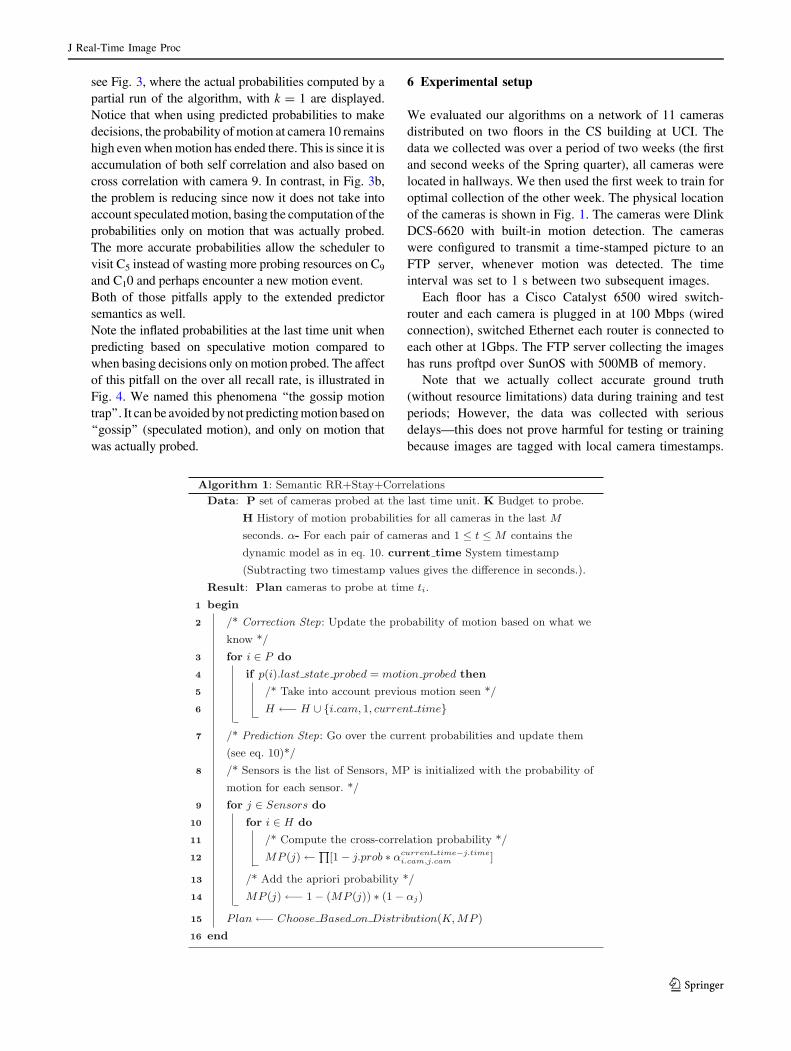
6 Experimental setup

We evaluated our algorithms on a network of 11 cameras

distributed on two floors in the CS building at UCI. The

data we collected was over a period of two weeks (the first

and second weeks of the Spring quarter), all cameras were

located in hallways. We then used the first week to train for

optimal collection of the other week. The physical location

of the cameras is shown in Fig. 1. The cameras were Dlink

DCS-6620 with built-in motion detection. The cameras

were configured to transmit a time-stamped picture to an

FTP server, whenever motion was detected. The time

interval was set to 1 s between two subsequent images.

Each floor has a Cisco Catalyst 6500 wired switch-

router and each camera is plugged in at 100 Mbps (wired

connection), switched Ethernet each router is connected to

each other at 1Gbps. The FTP server collecting the images

has runs proftpd over SunOS with 500MB of memory.

Note that we actually collect accurate ground truth

(without resource limitations) data during training and test

periods; However, the data was collected with serious

delays—this does not prove harmful for testing or training

because images are tagged with local camera timestamps.


123

Our end goal is to design a real-time scheduler which

avoids such delays using a semantic model.

Furthermore, each cameras was able to process the

images locally in hardware, sending only images contain-

ing motion. In a general setting where the sensors do not

have these local processing capabilities, scheduling

becomes a vital issue since a central server must also

perform motion detection for each time instant for each

camera.

We ran the evaluation on a Windows XP PC running

Oracle with Intel Pentium 4, 3.0 Mhz processor and 1Gb of

RAM.

6.1 Evaluation methodology

The training data were used to generate three tables: first

the probability of unconditioned motion for each camera

was computed and stored in a table. The cardinality of that

table is 11, one record per camera. Second, for each camera

we computed the self-correlation matrix, as discussed in

Sect. 4.2. The cardinality of this table was 11*4, four

values per sensor. Finally, we computed the correlation

between sensors (as discussed in Sect. 4.3.2), and stored

the correlations in a table of size 11*11*156.

To reduce the size of the correlation matrix, we did the

following: We computed a threshold probability, p = 0.05,

and removed all entries of less probability from the table.

This value to be visually verified by noting that in Fig. 1b

and c, everything below 0.05 is noise. Similarly, we found

that it is sufficient to look back only 15 s, when considering

correlations between different cameras.

The correlation matrix was not to be used for self-cor-

relation, which justified the removal of all entries where a

camera was self-correlated. Eventually, the cardinality of

the table containing these associations was 165 as opposed

to 1815 we started with7. The different algorithms were

implemented in PL/SQL. We simulated the different

algorithms, with varying budget: 1 B k B 11 by running it

over the test data. Each algorithm generated a plan to probe

k sensors based on the motion detected by the previous

probes. We counted the number of ‘‘hits’’ of each plan and

later computed the precision, recall, and relative

improvement in recall over round robin. Precision was

computed as the fraction of probes containing motion out

of the total number of probes. The recall was the fraction of

motion detected out of the whole motion in the system.

6.2 Evaluation results

With a budget of 1, our last two semantic algorithms

achieved over 150%(!) improvement over RR (see Fig. 5a).

‘‘RR ? Stay ? NN’’ performed much worse than

‘‘RR ? Stay’’. This proves that without exploiting

semantics properly, an ad-hoc approach will prove to

perform worse than a simple alternative(‘‘RR ? Stay’’),

which in this case better exploits the semantics of the data.

The probabilistic approach ‘‘Semantic RR’’ proved to

work better then RR but worse than all other alternatives

that took into account the continuation of motion.

‘‘Semantic RR ? Stay’’ is the ‘‘second-best’’ candidate

exploiting more of the available semantics than all other

alternatives and proves to achieve about 100% improve-

ment over the best out of the deterministic approaches.

‘‘Semantic RR ? Stay ? Correlations’’ and the model

exploiting extended semantics dominate the chart and offer

a tremendous improvement over all other alternatives,

when the resources are constrained.

To give an intuition for the reasons behind this vast

improvement, imagine that a sensor falsely detects that

there is no motion. The deterministic approaches would

choose to go to a different sensor, and will not be able to

‘‘recover’’ from that error. The probabilistic approaches

elegantly recover from that situation as the training data

teaches the algorithm that sometimes it is a good idea to

look back and check again for motion, as the probability

for motion will not drop to zero immediately after no

motion was detected (see Fig. 1c).

The Model with Extended Predictor Semantics, per-

formed almost the same as Semantic RR ? Stay ? corre-

lation in this case, when the benefit function is motion.

1 2 3 4 5 6 7 8 9 10 110

0.1

0.2

0.3

0.4

0.5

0.6

0.7

0.8

0.9

1

Budget

Rec

all o

f Mot

ion

Benefit Function − Motion

Semantic RR+Stay+CorrelationsSemantic RR+Stay+Correlations:GossipSemantic RR+Stay+Correlations:Top k

Fig. 4 The effect of the two pitfalls on the recall rate

6 which is n*n*M where n is the number of sensors and M is the time

window to look back.

7 The table size is 1262 after thresholding in the extended semantics

case, as opposed to 11*11*15*4 = 7, 260. The last 4 represents the

four states: event start, event ongoing, event end and motion.


123

Thus, the extra information didn’t improve the perfor-

mance of the scheduler when all motion events are equally

important. We will see a difference in Sect. 6.3 when we

score the performance of the scheduler based on different

benefit functions discussed next.

6.3 Experimenting with other scoring types

One might claim that the application might not benefit

from multiple motion events of the same person walking

down a long hallway, but rather from capturing as many

frames from different such individual trajectories.

In order to evaluate the performance of our approach in

this scenario we created a notion of a continuous event as

follows: we ran a connected component analysis over the

motion stream to generate continuous motion events. To

illustrate, the following motion pattern at a single sensor:

.. - ? ? - ? ? ? - .. would generate two motion

events, of length 2 and 3. Given these motion events we are

able to define different scoring functions (benefit

functions):

• Distinct events as the number of distinct events that

were probed.

• Motion start time as the first second of the motion burst.

• Delay as the number of seconds elapsed from the start

time of the event until the first probe.

Next, we report the recall rates based on these different

scoring function.

6.3.1 Distinct events

When the number of different events found is counted

(Fig. 6b) we can see the benefit of using the model with

extended semantics, as the recall rate improves even

compared to Semantic RR ? Stay ? Correlation. The

number of distinct events that the scheduler was able to

probe was 45% higher compared to RR with k = 1.

Semantic RR ? Stay ? Correlation achieved a 34%

improvement over RR.

The best Semantic algorithms dominate all other algo-

rithms but the improvement in this case was smaller than

what was found in the case of motion—Semantic

RR ? Stay ? Correlation was only able to get 35%

improvement over RR with k = 1 and 15% with K = 2.

The reason that RR proves to be a reasonable strategy is

that long lasting events, have a very high probability of

being probed once by RR. Even with a budget of 1, in our

case, RR will hit on all events of length 11 or more. With

budget of k ¼ n2

RR will visit every camera every two

seconds and achieve very high recall rates (all events of

length 2 or more will be captured). This leaves a very small

slack for improvement. An improvement of any algorithm

over RR, under this scoring function is only when k ¼ np

and p ¼ nk is greater than the average length of motion

events. In our system events on average last 2.65 s, we

would expect to see almost no improvement over RR when

kC4.15. This is supported by our results: as we see no

improvement when kC5.

Notice that it is possible to do much worse than RR,

actually, RR ? Stay ? NN performs considerably worse

than RR. The reason is that this algorithm will choose to

continuously probe a sensor (Stay) which serves no benefit

to capture distinct events. The ‘‘hard-coded’’ rule of staying

in a neighboring sensor until motion begins serves as

another factor which decreases the recall of different

events.

1 2 3 4 5 6 7 8 9 10 110

20

40

60

80

100

120

140

160

180

BudgetPer

cent

age

of Im

prov

emen

t in

Rec

all,

Com

pare

d to

RR Benefit Function Motion

RRRR+StayRR+Stay+NNSemantic RRSemantic RR+StaySemantic RR+Stay+CorrelationsExtended Semantics

(a)

1 2 3 4 5 6 7 8 9 10 110

0.1

0.2

0.3

0.4

0.5

0.6

0.7

0.8

0.9

1

Budget

Rec

all

Benefit Function Motion


(b)

Fig. 5 Comparison of the different algorithms—motion hits.

a Improvement over RR, b Recall


123

6.3.2 Average delay

An alternative to different events would be to measure the

‘‘responsiveness’’ of the system in terms of the average

number of seconds that pass from the beginning of the event

until the algorithm probes it. Again, the richer model was able

to outperform all other methods, the delay shortened on

average on 8% compared to Semantic RR ? Stay ? Corre-

lation. Semantic RR ? Stay ? Correlation achieves 40–80%

decrease in the average delay time compared to RR. The

reason is that RR simply ‘‘guesses’’ where to go next, while

the semantic algorithms incorporate information about where

motion is expected to start and probe sensors in an informed

systematic fashion leading to better responsiveness.

RR ? Stay ? NN is comparable only when k = 1, which is

explained by it probing nearest neighbors which other algo-

rithms, except the semantic algorithms that incorporate cross

correlations, do not. When k increases, RR ? Stay ? NN

quickly loses its dominance and the reason is that its decision

making is not accurate, e.g., wait 60 s in the nearest neighbor.

The best semantic elegantly incorporates all the available

semantic information and efficiently exploits it. Moreover,

notice that RR ? Stay ? NN has a much smaller recall rete

of distinct events compared to the best semantic algorithm.

Although it achieves a good average response time for k = 1,

the recall rate of events is smaller. The semantic algorithm

with extended predictor semantics dominates the chart as it

uses information about the end of events to accurately predict

the start of events as opposed to treating all events as motion

events (Fig. 7).

1 2 3 4 5 6 7 8 9 10 110

0.2

0.4

0.6

0.8

1

1.2

1.4

Budget

Ave

rage

Del

ay in

Sec

onds

Benefit Function Average Delay


1 2 3 4 5 6 7 8 9 10 11–90

–80

–70

–60

–50

–40

–30

–20

–10

0

10

BudgetPer

cent

age

of Im

prov

emen

t in

Ave

rage

Del

ay, C

ompa

red

to R

R Benefit Function Average Delay

(a)

(b)

Fig. 7 Comparison of the different algorithms—average delay scor-

ing function. a Average delay in seconds, b average delay compared

to the recall of RR

1 2 3 4 5 6 7 8 9 10 110.1

0.2

0.3

0.4

0.5

0.6

0.7

0.8

0.9

1

Budget

Rec

all o

f Dis

tinct

Eve

nts

Benefit Function Distinct Events


1 2 3 4 5 6 7 8 9 10 11–40

–30

–20

–10

0

10

20

30

40

50

BudgetPer

cent

age

of Im

prov

emen

t in

Rec

all,

Com

pare

d to

RR Benefit Function Distinct Events


(a)

(b)

Fig. 6 Comparison of the different algorithms—different events

scoring function. a Recall of different events, b recall compared to the

recall of RR


123

6.3.3 Event start

The semantic algorithm with extended predictor semantics

was able to get a considerable improvement over semantic

RR ? Stay ? Correlation, over 20% improvement for

k = 1 and about 8% on average for k [ 1. Semantic

RR ? Stay ? Correlation achieved about 100% improve-

ment over RR with K = 1, K = 2 and a considerable

improvement over all other algorithms. This goes hand in

hand with the results for number of distinct events and

average delay. This result is extremely important for cases

where the sensors are located close to entry/exit points as

the first frame is expected to contain the highest quality of

picture of an individual that just walk in the field of view of

the camera (Fig. 8).

6.3.4 Experimenting with other scoring types—summary

Overall, the best semantic algorithm achieves the best

results, compared to all other algorithms. Even in the case

where RR performs relatively well (different events) the

best semantic is still the best choice.

So far we evaluated the algorithm based on different

benefit functions, and the decision was always to probe

based on where motion is most likely to happen (best

semantic). It is part of our planned future work to inves-

tigate an alternative approach which will probe the sensors

based a function of the predicted probabilities. For exam-

ple, for different events, it seems that once we saw motion

for a particular sensor, probing it again at the next time unit

would serve no purpose, as it is expected that the next time

unit will contain a motion event—part of the one already

detected.

As an example of such function we probabilities are

computed as before but are used for probing as follows: for

each sensor we estimated the probability that motion in the

next time unit is a continuation of a previously observed

motion event, Pmotion seen already. The last can be obtained

computing the probability of the HMM associated with that

sensor staying at state motion for the time interval since it

was last probed to be in motion state.

Next subtract from the computed probability of motion

Pmotion seen already and use the computed probabilities to

schedule the next set of probes. This alternative was able to

meet the performance of our best semantic algorithm but

not improve on it.

The intuition behind the difficulty of that problem is that

probing a sensor again, although not serving the benefit

function immediately, is important for accurate state esti-

mation. Since motion events are used to predict future

motion events it is important to keep an accurate state

estimation—which serves the benefit function indirectly.

The challenge is to design an algorithm that would find the

optimal balance between probing for state estimation and

probing for the benefit of the application.

7 Conclusions and future work

In this paper, we address the challenge of scheduling data

collection from sensors to maximize event detection. We

designed and implemented a fully functional system using

available off-the-shelf cameras to learn motion semantics

for our building and evaluated different scheduling algo-

rithms based on non scripted motion over a period of a

week. Our semantic based algorithm that takes into account

all available semantic information proves that even under

significant resource constraints, we can detect a very large

number of events.

1 2 3 4 5 6 7 8 9 10 110

0.1

0.2

0.3

0.4

0.5

0.6

0.7

0.8

0.9

1

Budget

Rec

all o

f the

Sta

rt o

f Eve

nts

Benefit Function Event Start


1 2 3 4 5 6 7 8 9 10 11–20

0

20

40

60

80

100

120

140

Budget% Im

prov

emen

t in

Rec

all o

f the

Sta

rt o

f Eve

nts,

Com

pare

d to

RR Benefit Function Event Start


(a)

(b)

Fig. 8 Comparison of the different algorithms—event start scoring

function. a Recall of events start, b recall compared to recall of RR


123

We followed a pull based approach, however, for future

work plan to investigate a hybrid push/pull approach that

will benefit from the advantages of computation at the

sensors while meeting the deadlines of a real-time system

and supporting the dynamic nature of a surveillance task.

We started this work stating five assumptions. In our

future work, we plan to relax these assumptions. Semantics

available: we will extract features from the images, such as

number of people in the FOV learn semantic information

based on such information and use semantics at different

levels (motion, number of people) for scheduling. In this

work, we already incorporated semantics at two different

levels: motion and event type (event start, end or ongoing).

Updating the semantic model while the system is in opera-

tion, up-to-date information is collected about the state of

the system. This information can be used to tune the

semantic model, for example, due to changes in the semantic

behavior (A new coffee-machine was installed and more

people tended to stop for coffee). This problem relates to a

problem addressed by the database communities: estimating

query selectivity based on the actual query results [3]. We

plan to study the affect of different prediction windows on

the recall rates of our algorithms. The scheduler will be

given the state of the system as was ‘‘seen’’ in the last t

seconds, and will generate a plan for the next t seconds. At

that stage, distributed decision making might be taken into

account as each node might choose to ‘‘stay’’ when motion is

‘‘seen’’ and further ‘‘tip’’ a correlated node to expect as

opposed to being loyal to an obsolete plan. Note that our

current algorithms can scale with large number of sensor as

semantics are local and several decision making nodes can

operate in parallel, e.g., we could have installed a different

scheduler for each floor in out building case. Different cost

functions that depend on the actual network topology, delays

and connection overheads is in our plan to relax the

homogenous assumption.

Acknowledgments Support of this research by the National Science

Foundation under Award Numbers 0331707 and 0331690 and the

Department of Homeland Security under award number EMW-2007-

FP-02535 is gratefully acknowledged.

References

1. Anandathirtha, P., Ramakrishnan, K., Raja, S., Kankanhalli, M.:

Experiential sampling for object detection in video. In: Multi-

media Content Analysis: Theory and Applications, p. 175 (2009)

2. Brown, R.G., Hwang, P.Y.C.: Introduction to Random Signals

and Applied Kalman Filtering. Wiley, New York (1992)

3. Chen, C., Roussopoulos, N.: Adaptive selectivity estimation using

query feedback. In: Proceedings of the 1994 ACM SIGMOD Inter-

national Conference on Management of Data, pp. 161–172 (1994)

4. Daeipour, E., Bar-Shalom, Y.: An interacting multiple model

approach for target tracking withglint noise. IEEE Trans. Aerosp.

Electr. Syst. 31(2), 706–715 (1995)

5. Gupta, V., Chung, T., Hassibi, B., Murray, R.: On a stochastic

sensor selection algorithm with applications in sensor scheduling

and sensor coverage. Automatica 42(2), 251–260 (2006)

6. Han, Q., Mehrotra, S., Venkatasubramanian, N.: Energy efficient

data collection in distributed sensor environments. In: Proceed-

ings of 24th International Conference on Distributed Computing

Systems, vol. 39, pp. 590–597 (2004)

7. Ihler, A., Hutchins, J., Smyth, P.: Adaptive event detection with

time-varying poisson processes. In: KDD ’06: Proceedings of the

12th ACM SIGKDD International Conference on Knowledge

Discovery and Data Mining, pp. 207–216. ACM Press, New York

(2006). doi:10.1145/1150402.1150428

8. Isler, V., Bajcsy, R.: The sensor selection problem for bounded

uncertainty sensing models. In: IPSN 2005 Fourth International

Symposium on Information Processing in Sensor Networks,

2005, pp. 151–158 (2005)

9. Kao, B., Garcia-Molina, H.: Deadline assignment in a distributed

soft real-time system. IEEE Trans. Parallel Distrib. Syst. 8(12),

1268–1274 (1997)

10. Krishnamurthy, V.: Algorithms for optimal scheduling and

management of hidden Markovmodel sensors. IEEE Trans. Sig-

nal Process. [see also IEEE Trans. Acoust. Speech Signal Pro-

cess.] 50(6), 1382–1397 (2002)

11. Lazaridis, I., Mehrotra, S.: Capturing sensor-generated time ser-

ies with quality guarantees. In: International Conference on Data

Engineering (ICDE) (2003)

12. Makris, D., Ellis, T., Black, J.: Bridging the gaps between cam-

eras. In: CVPR 2004 Proceedings of the 2004 IEEE Computer

Society Conference on Computer Vision and Pattern Recogni-

tion, vol. 2 (2004)

13. Murphy, K.P., Weiss, Y.: The factored frontier algorithm for

approximate inference in dbns. In: UAI ’01: Proceedings of the

17th Conference in Uncertainty in Artificial Intelligence, pp.

378–385. Morgan Kaufmann Publishers Inc., San Francisco

(2001)

14. Nieh, J., Lam, M.: The design, implementation and evaluation of

SMART: a scheduler for multimedia applications. In: Proceed-

ings of the Sixteenth ACM Symposium on Operating Systems

Principles, pp. 184–197. ACM, New York (1997)

15. Pearl, J.: Probabilistic Reasoning in Intelligent Systems: Net-

works of Plausible Inference. Morgan Kaufmann Publishers Inc.,

San Francisco (1988)

16. Rabiner, L.R.: A tutorial on hidden markov models and selected

applications in speech recognition. Proc. IEEE 77(2), 257–286

(1989)

17. Schulz, D., Fox, D., Hightower, J.: People tracking with anony-

mous and id-sensors using rao-blackwellised particle filters. In:

Proceedings of the International Joint Conference on Artificial

Intelligence (IJCAI) (2003)

18. Scott, S.: Detecting network intrusion using a Markov modulated

nonhomogeneous Poisson process. J. Am. Stat. Assoc. (2010)

19. Song, B., Roy-Chowdhury, A.: Stochastic adaptive tracking in a

camera network. In: IEEE 11th International Conference on

Computer Vision, 2007 ICCV, pp. 1–8 (2007)

20. Vaisenberg, R., Mehrotra, S., Ramanan, D.: Exploiting semantics for

scheduling real-time data collection from sensors to maximize event

detection. In: Proceedings of SPIE, vol. 7253, p. 72530B (2009)

21. Williams, J., Fisher, J. III, Willsky, A.: An approximate dynamic

programming approach to a communication constrained sensor

management problem. In: Proceedings of Eighth International

Conference of Information Fusion (2005)

22. Yu, X., Niyogi, K., Mehrotra, S., Venkatasubramanian, N.:

Adaptive target tracking in sensor networks. In: Communication

Networks and Distributed Systems Modeling and Simulation

Conference (CNDS04) (2004)


123

http://dx.doi.org/10.1145/1150402.1150428

semartcam scheduler: semantics driven real-time data collection

Documents