semantic information extraction of lanes based on onboard …

SEMANTIC INFORMATION EXTRACTION OF LANES BASED ON ONBOARD

CAMERA VIDEOS

Luliang Tang 1, Tuo Deng 1, *, Chang Ren 1

1 State Key Laboratory of Information Engineering in Surveying, Mapping, and Remote Sensing, Wuhan University, Wuhan, China -

(tll, dengtuo, imrc)@whu.edu.cn

Commission III, WG III/1

KEY WORDS: Lane Marking Detection, Lane Semantic Recognition, Lane Classification, Onboard Camera Video, Lane-Based

Road Network

ABSTRACT:

In the field of autonomous driving, semantic information of lanes is very important. This paper proposes a method of automatic

detection of lanes and extraction of semantic information from onboard camera videos. The proposed method firstly detects the

edges of lanes by the grayscale gradient direction, and improves the Probabilistic Hough transform to fit them; then, it uses the

vanishing point principle to calculate the lane geometrical position, and uses lane characteristics to extract lane semantic information

by the classification of decision trees. In the experiment, 216 road video images captured by a camera mounted onboard a moving

vehicle were used to detect lanes and extract lane semantic information. The results show that the proposed method can accurately

identify lane semantics from video images.

* Corresponding author

1. INTRODUCTION

High-precision lane-level road maps provides information such

as lane number, location, geometry and connectivity semantic,

and its acquisition of low cost is a focus and difficulty in the

field of autonomous driving (Hillel et al, 2014). There are

several existing methods for obtaining lane-level road

information: such as using high resolution images to extract the

centerline markings and the width of lanes (Ye et al, 2006; Cao

et al, 2017; Yu et al, 2013; Lisini 2006); using

airborne/terrestrial Lidar data to extract the edge, road markings

and geographic position of lanes(Fang et al, 2013; Anttoni et al,

2008; Hui et al, 2016); using GPS trajectories to extract the

number, location, and change detection of lanes(Chen et al,

2010; Tang et al, 2016; Yang et al, 2017). The above lane-level

road data acquisition methods have the disadvantages of high

cost, slow update, lack of semantic information, so it is urgent

to develop a method with low cost, quick collection, and

complete road information.

With the rapid development of sensors and Internet of Things

technologies, more and more vehicle users have installed

onboard cameras. These videos produced huge amounts of

video data, containing rich road markings and lane semantic

information such as speed limit signs, lane direction, and

turning information (Yeh et al, 2015). Therefore, onboard

camera videos data provides a rich data source for lane-level

road information extraction with fast acquisition, low cost, and

complete semantic information, which provides important

technical support for vehicle navigation, driving assistance

system, and autonomous driving. The onboard camera videos

are mainly used for lane detection in driving assistance system

in the existing research (Aly, 2008; Paula et al, 2013; Chen et al,

2011). There is less research on lane semantic recognition. This

paper proposes a method of extracting lane position and

semantic information by using onboard camera videos.

2. TYPE OF LANE MARKINGS

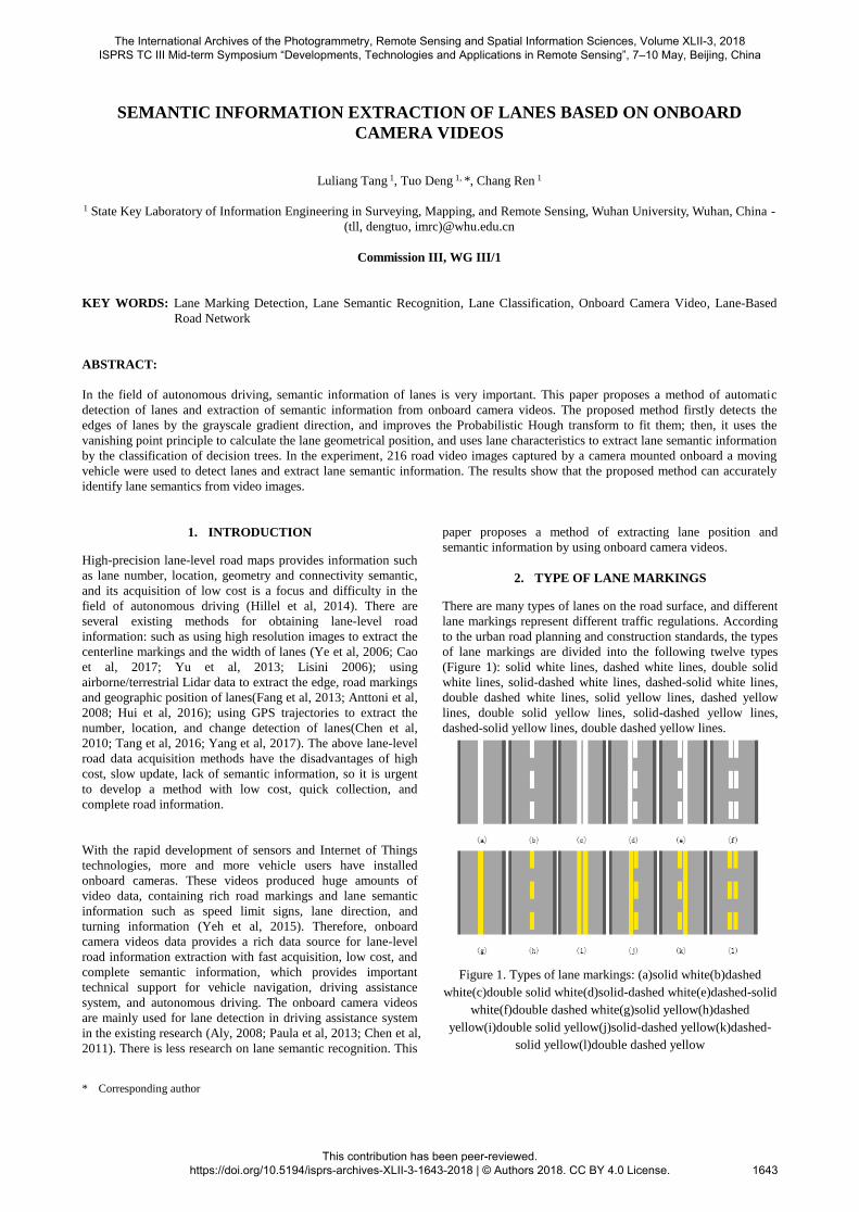
There are many types of lanes on the road surface, and different

lane markings represent different traffic regulations. According

to the urban road planning and construction standards, the types

of lane markings are divided into the following twelve types

(Figure 1): solid white lines, dashed white lines, double solid

white lines, solid-dashed white lines, dashed-solid white lines,

double dashed white lines, solid yellow lines, dashed yellow

lines, double solid yellow lines, solid-dashed yellow lines,

dashed-solid yellow lines, double dashed yellow lines.

Figure 1. Types of lane markings: (a)solid white(b)dashed

white(c)double solid white(d)solid-dashed white(e)dashed-solid

white(f)double dashed white(g)solid yellow(h)dashed

yellow(i)double solid yellow(j)solid-dashed yellow(k)dashed-

solid yellow(l)double dashed yellow

The International Archives of the Photogrammetry, Remote Sensing and Spatial Information Sciences, Volume XLII-3, 2018 ISPRS TC III Mid-term Symposium “Developments, Technologies and Applications in Remote Sensing”, 7–10 May, Beijing, China

This contribution has been peer-reviewed. https://doi.org/10.5194/isprs-archives-XLII-3-1643-2018 | © Authors 2018. CC BY 4.0 License.

1643

In general, white lines always separates traffic in the same

direction while yellow lines separates the inverse. Single dashed

lines mean passing or lane changing is allowed, single solid

white lines mean lane changing is discouraged but not

prohibited, and double solid white lines mean it is prohibited.

On two-lane roads, a single dashed centerline means that

passing is allowed in either direction, a double solid centerline

means passing is prohibited in both directions, and the

combination of a solid line with a dashed line means that

passing is allowed only from the side with the broken line and

prohibited from the side with the solid line.

3. SEMANTIC INFORMATION EXTRACTION OF

LANES

3.1 Lane Markings Detection Based on Videos

Detecting lane markings is the basis of extracting lane semantic

information, so the first step of the proposed approach is to

detect lane boundaries from video images. To simplify

complicated lane detection problem, we assume the following

conditions: (1) strong image noise does not exist; (2) the road

width is fixed or changes slowly and the road plane is flat; (3)

the camera frame axis stays parallel to the road frame plane.

These assumptions can improve the effectiveness and real-time

performance of the detection algorithm.

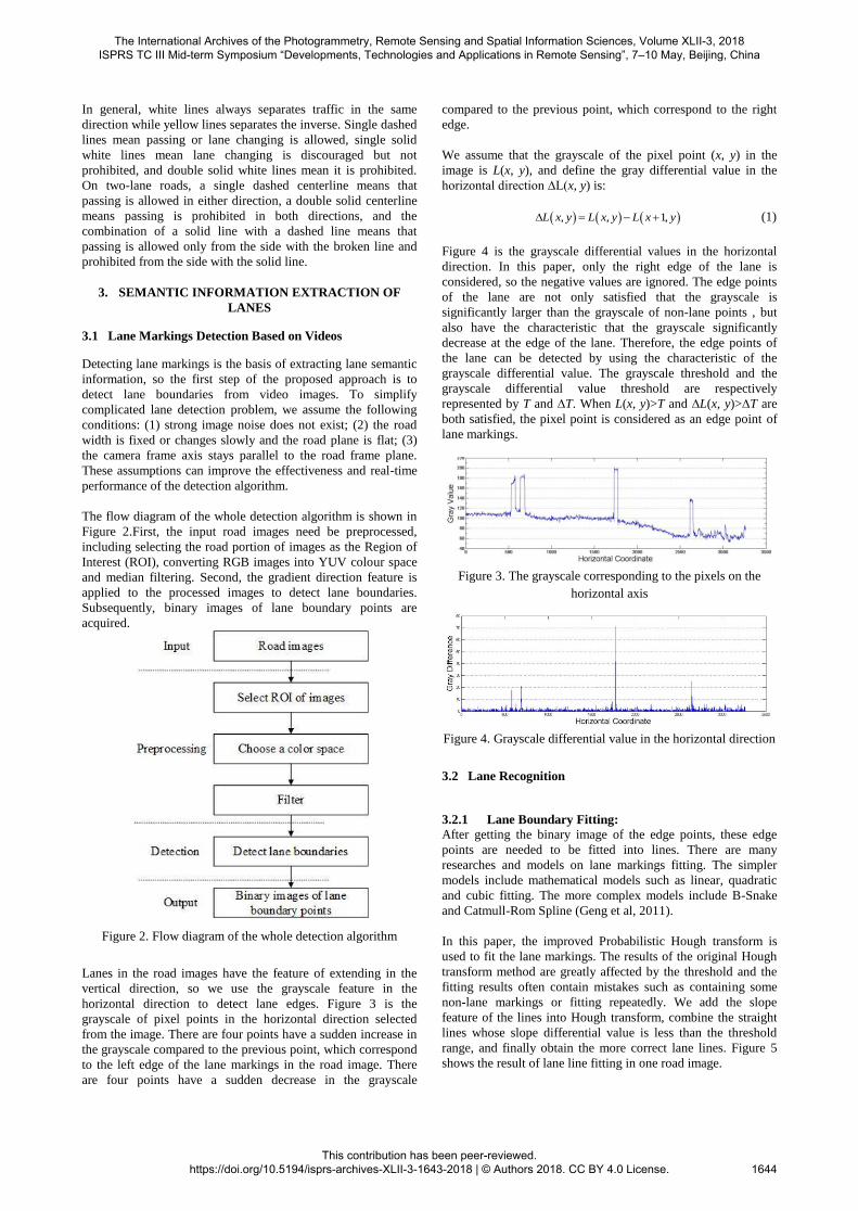
The flow diagram of the whole detection algorithm is shown in

Figure 2.First, the input road images need be preprocessed,

including selecting the road portion of images as the Region of

Interest (ROI), converting RGB images into YUV colour space

and median filtering. Second, the gradient direction feature is

applied to the processed images to detect lane boundaries.

Subsequently, binary images of lane boundary points are

acquired.

Figure 2. Flow diagram of the whole detection algorithm

Lanes in the road images have the feature of extending in the

vertical direction, so we use the grayscale feature in the

horizontal direction to detect lane edges. Figure 3 is the

grayscale of pixel points in the horizontal direction selected

from the image. There are four points have a sudden increase in

the grayscale compared to the previous point, which correspond

to the left edge of the lane markings in the road image. There

are four points have a sudden decrease in the grayscale

compared to the previous point, which correspond to the right

edge.

We assume that the grayscale of the pixel point (x, y) in the

image is L(x, y), and define the gray differential value in the

horizontal direction ∆L(x, y) is:

, , 1,L x y L x y L x y (1)

Figure 4 is the grayscale differential values in the horizontal

direction. In this paper, only the right edge of the lane is

considered, so the negative values are ignored. The edge points

of the lane are not only satisfied that the grayscale is

significantly larger than the grayscale of non-lane points , but

also have the characteristic that the grayscale significantly

decrease at the edge of the lane. Therefore, the edge points of

the lane can be detected by using the characteristic of the

grayscale differential value. The grayscale threshold and the

grayscale differential value threshold are respectively

represented by T and ∆T. When L(x, y)>T and ∆L(x, y)>∆T are

both satisfied, the pixel point is considered as an edge point of

lane markings.

Figure 3. The grayscale corresponding to the pixels on the

horizontal axis

Figure 4. Grayscale differential value in the horizontal direction

3.2 Lane Recognition

3.2.1 Lane Boundary Fitting:

After getting the binary image of the edge points, these edge

points are needed to be fitted into lines. There are many

researches and models on lane markings fitting. The simpler

models include mathematical models such as linear, quadratic

and cubic fitting. The more complex models include B-Snake

and Catmull-Rom Spline (Geng et al, 2011).

In this paper, the improved Probabilistic Hough transform is

used to fit the lane markings. The results of the original Hough

transform method are greatly affected by the threshold and the

fitting results often contain mistakes such as containing some

non-lane markings or fitting repeatedly. We add the slope

feature of the lines into Hough transform, combine the straight

lines whose slope differential value is less than the threshold

range, and finally obtain the more correct lane lines. Figure 5

shows the result of lane line fitting in one road image.



1644

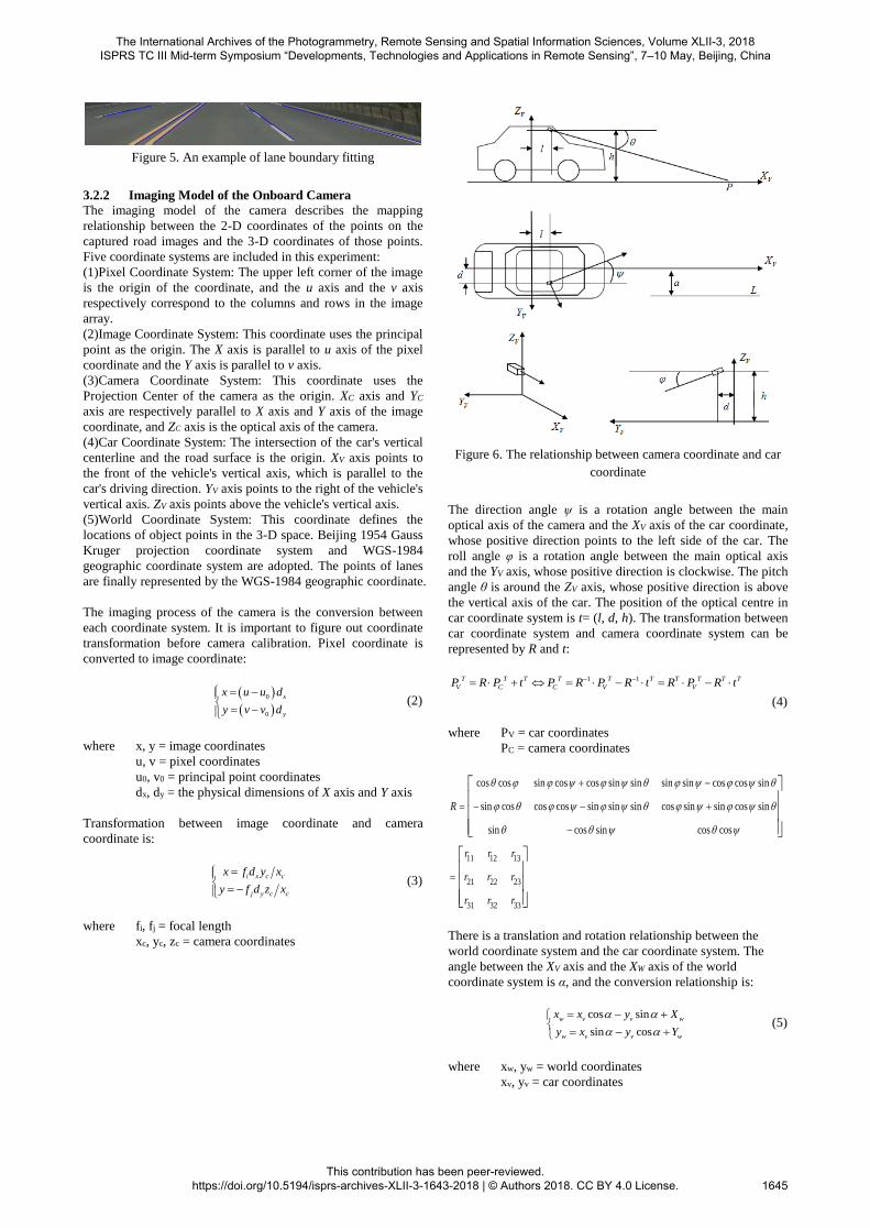
Figure 5. An example of lane boundary fitting

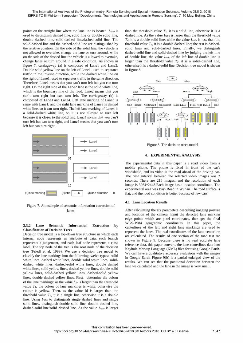
3.2.2 Imaging Model of the Onboard Camera

The imaging model of the camera describes the mapping

relationship between the 2-D coordinates of the points on the

captured road images and the 3-D coordinates of those points.

Five coordinate systems are included in this experiment:

(1)Pixel Coordinate System: The upper left corner of the image

is the origin of the coordinate, and the u axis and the v axis

respectively correspond to the columns and rows in the image

array.

(2)Image Coordinate System: This coordinate uses the principal

point as the origin. The X axis is parallel to u axis of the pixel

coordinate and the Y axis is parallel to v axis.

(3)Camera Coordinate System: This coordinate uses the

Projection Center of the camera as the origin. XC axis and YC

axis are respectively parallel to X axis and Y axis of the image

coordinate, and ZC axis is the optical axis of the camera.

(4)Car Coordinate System: The intersection of the car's vertical

centerline and the road surface is the origin. XV axis points to

the front of the vehicle's vertical axis, which is parallel to the

car's driving direction. YV axis points to the right of the vehicle's

vertical axis. ZV axis points above the vehicle's vertical axis.

(5)World Coordinate System: This coordinate defines the

locations of object points in the 3-D space. Beijing 1954 Gauss

Kruger projection coordinate system and WGS-1984

geographic coordinate system are adopted. The points of lanes

are finally represented by the WGS-1984 geographic coordinate.

The imaging process of the camera is the conversion between

each coordinate system. It is important to figure out coordinate

transformation before camera calibration. Pixel coordinate is

converted to image coordinate:

0

0

x

y

x u u d

y v v d

(2)

where x, y = image coordinates

u, v = pixel coordinates

u0, v0 = principal point coordinates

dx, dy = the physical dimensions of X axis and Y axis

Transformation between image coordinate and camera

coordinate is:

i x c c

j y c c

x f d y x

y f d z x

(3)

where fi, fj = focal length

xc, yc, zc = camera coordinates

Figure 6. The relationship between camera coordinate and car

coordinate

The direction angle ψ is a rotation angle between the main

optical axis of the camera and the XV axis of the car coordinate,

whose positive direction points to the left side of the car. The

roll angle φ is a rotation angle between the main optical axis

and the YV axis, whose positive direction is clockwise. The pitch

angle θ is around the ZV axis, whose positive direction is above

the vertical axis of the car. The position of the optical centre in

car coordinate system is t= (l, d, h). The transformation between

car coordinate system and camera coordinate system can be

represented by R and t:

1 1T T T T T T T T T T

V C C V VP R P t P R P R t R P R t

(4)

where PV = car coordinates

PC = camera coordinates

12 13

21 23

3

11

22

32 331

cos cos sin cos cos sin sin sin sin cos cos sin

sin cos cos cos sin sin sin cos sin sin cos sin

cos sin cos cn ossi

r

r

r

r

r r

r r

R

r

There is a translation and rotation relationship between the

world coordinate system and the car coordinate system. The

angle between the XV axis and the XW axis of the world

coordinate system is α, and the conversion relationship is:

cos sin

sin cos

w v v w

w v v w

x x y X

y x y Y

(5)

where xw, yw = world coordinates

xv, yv = car coordinates



1645

(Xw, Yw) can be obtained by the camera. Α can be calculated by

two adjacent images:

2 1

2 1

arctan w w

w w

Y Y

X X

(6)

where Xw1, Yw1 = the current image coordinates

Xw2, Yw2 = the next image coordinates

3.2.3 Calculate the Position of Lanes

There are six parameters describing imaging posture and

location of the camera: 3 rotation angle- direction angle ψ, roll

angle φ and pitch angle θ, and 3 translation components- l, d

and h. This paper uses the vanishing point principle to calibrate

camera parameters and does not require a specific calibration

field. In accordance with the perspective projection principle of

camera, three mutually non-coincident parallel lines have same

vanishing point and different slopes on imaging plane (Li et al,

2004).Thus, the external parameters of the camera can be

represented by a mathematical expression associated with

parallel lane markings and vanishing point.

For a random line L parallel to the XV axis, if the distance from

L to XV is a, the equation in the car coordinate system can be

expressed as:

, , 0v v vx s y a z (7)

where a = any real number

To image this line, it needs to be transformed into the camera

coordinate system. From (4), the equation of L in the camera

coordinate system is:

11 21 31 11 21 31

12 22 32 12 22 32

13 23 33 13 23 330

c

c

c

x r r r s r r r l

y r r r a r r r d

z r r r r r r h

(8)

Finally, it is transformed into image coordinate system. From (3)

and (8), the equation of L in the image coordinate system is:

12 22 12 22 32 11 21 11 21 31

13 23 13 23 33 11 21 11 21 31

/

/

i x

j y

x f d sr ar lr dr hr sr ar lr dr hr

y f d sr ar lr dr hr sr ar lr dr hr

(9)

The vanishing point of L in the image coordinate system is (uh,

vh). Because s is an any real number and the distance between

the optical center of the camera in XV axis is l, there is an any

real number after andding or subtracting between s and l:

lim sin cos cos sin sin / cos cos

lim sin sin cos cos sin / cos cos

h i xs

h j ys

u u f d

v v f d

(10)

If there are at least three lane markings parallel to XV on the

road surface, the distance between them and XV axis is a1, a2

and a3. Their vanishing point is:

1 2 3 1 2 3h h h h h h h hu u u u v v v v ， (11)

The slope of the three lines can be computed:

12 21 12 21 12 31 11 22 11 22 11 32

13 21 13 21 13 31 11 23 11 23 11 33

i x nn

j y n

f d a r r dr r hr r ar r dr r hr rg

f d a r r dr r hr r ar r dr r hr r

n=1, 2, 3… (12)

Rotation angles ψ, φ and θ, and translation components l, d and

h can be computed:

1 3 1 2 1 2 1 3 1 3 1 1 3 2 1 2 1 1 3 3

2 1

2 1 1

/

sin / cos /

cos / sin / cos

/

/ /

h i x h j y

h i x

arctg r r a a r r a a r r r a r a r r r a r a

arctg u f d v f d

arctg u f d tg

h a a AC BC AD

d B A a a AC BC AD a

(13)

where 1A sin cos cos cosr

1cos sin sin cos sin cos cos sin sin sinB r

2 sin cos cos cosC r

2cos sin sin cos sin cos cos sin sin sinD r

/ / , 1,2,3...n j i h n h nr f f i i j j n

From(13), when we know the camera internal parameters fi, fj

and u0,v0, the distance between any three lane markings on

video images in the car coordinate system and XV axis- a1, a2

and a3, and any other points on the three lanes in pixel

coordinate system, the external parameters of camera can be

calculated.

When calibration parameters of the camera are calculated, we

can calculate the position of lane points by the coordinate

transformation. On the assumption of flat road plane (zv=0), we

can get from (4) and (9):

31 32 33/ / /

/

/

c i x j y

c c i x

c c j y

x h r r u f d r v f d

y x u f d

z x v f d

(14)

The coordinates of the lane points in the car coordinate system:

11 31 32 33 12 13

21 31 32 33 22 23

/ / / / /

/ / / / /

v i x j y c i x c j y

v i x j y c i x c j y

x r h r r u f d r v f d r x u f d r x v f d l

y r h r r u f d r v f d r x u f d r x v f d d

(15)

3.3 Semantic Information Extraction of Lanes

3.3.1 Lane Characteristics Analysis

The lane semantic information is obtained according to the

types of lane markings. Lane markings have colour features,

single or double line features, and dashed or solid line features.

The traffic semantics represented by different types of lane

markings are different. The two colours of the lines are white

and yellow. It is found that the Cb component value of the

yellow lane line under various lighting conditions is the

smallest. So the Cb component ICb in the YCbCr colour space

of the lane edge points can identify the colour. The white line is

usually the dividing line between lanes running in the same

direction, and the yellow line is the dividing line between lanes

that drive in opposite directions. In order to distinguish single

line or double line, it is necessary to use the actual distance

value Id of the lane to judge. Define a ratio Iratio, which means

that the number of points on each lane line in the road binary

image with the value of 255 is divided by the number of all



1646

points on the straight line where the lane line is located. Iratio is

used to distinguish dashed line, solid line or double solid line,

double dashed line, solid-dashed line/dashed-solid line. The

solid-dashed line and the dashed-solid line are distinguished by

the relative position. On the side of the solid line, the vehicle is

not allowed to overtake, change the lane or turn around, while

on the side of the dashed line the vehicle is allowed to overtake,

change lanes or turn around in a safe condition. As shown in

figure 7, carriageway (a) is composed of Lane1 and Lane2.

Double solid yellow line on the left of Lane1, used to separates

traffic in the inverse direction, while the dashed white line on

the right of Lane1, used to separates traffic in the same direction.

Therefore, Lane1 means that you can’t turn left but you can turn

right. On the right side of the Lane2 lane is the solid white line,

which is the boundary line of the road. Lane2 means that you

can’t turn right but can turn left. The carriageway (b) is

composed of Lane3 and Lane4. Left lane marking of Lane3 is

same with Lane1, and the right lane marking of Lane3 is dashed

white line, so it can turn right. The left lane marking of Lane4 is

a solid-dashed white line, so it is not allowed to turn left

because it is closer to the solid line. Lane3 means that you can’t

turn left but can turn right, and Lane4 means that you can’t turn

left but can turn right.

Figure 7. An example of semantic information extraction of

lanes

3.3.2 Lane Semantic Information Extraction by

Classification of Decision Trees

Decision tree model is a top-down tree structure in which each

internal node represents an attribute of data, each branch

represents a judgement, and each leaf node represents a class

label. The top node of the tree is the root node of the decision

tree (Friedl et al, 1999). We use a decision tree model to

classify the lane markings into the following twelve types: solid

white lines, dashed white lines, double solid white lines, solid-

dashed white lines, dashed-solid white lines, double dashed

white lines, solid yellow lines, dashed yellow lines, double solid

yellow lines, solid-dashed yellow lines, dashed-solid yellow

lines, double dashed yellow lines. First，determine the colour

of the lane markings: as the value ICb is larger than the threshold

value T1, the colour of lane markings is white, otherwise the

colour is yellow. Then, as the value Id is larger than the

threshold value T2, it is a single line, otherwise it is a double

line. Using Iratio to distinguish single dashed lines and single

solid lines, distinguish double solid line, double dashed line,

dashed-solid line/solid–dashed line. As the value Iratio is larger

than the threshold value T3, it is a solid line, otherwise it is a

dashed line. As the value Iratio is larger than the threshold value

T4, it is a double solid line; while the value Iratio is less than the

threshold value T5, it is a double dashed line; the rest is dashed-

solid lines and solid-dashed lines. Finally, we distinguish

dashed-solid line and solid-dashed line by judging the left line

of double line, the value Iratio of the left line of double line is

larger than the threshold value T3, it is a solid–dashed line,

otherwise it is a dashed-solid line. Decision tree model is shown

in figure 8.

Figure 8. The decision trees model

4. EXPERIMENTAL ANALYSIS

The experimental data in this paper is a road video from a

mobile phone. The phone is fixed in front of the car's

windshield, and its video is the road ahead of the driving car.

The time interval between the selected video images was 2

seconds. There are 216 images, and the resolution of each

image is 3264*2448.Each image has a location coordinate. The

experimental area was Bayi Road in Wuhan. The road surface is

flat, and the road condition is better because of few cars.

4.1 Lane Location Results

After calculating the six parameters describing imaging posture

and location of the camera, input the detected lane marking

edge points which are pixel coordinates, then get the final

WGS-1984 geographic coordinates. In this paper, the

centerlines of the left and right lane markings are used to

represent the lanes. The real coordinates of the lane centerline

are calculated. The results of one section of the road test are

shown in Figure 9. Because there is no real accurate lane

reference data, this paper converts the lane centerlines data into

Keyhole Markup Language (KML) files for using Google Earth.

We can have a qualitative accuracy evaluation with the images

in Google Earth. Figure 9(b) is a partial enlarged view of the

results. We can see that the positional deviation between the

lane we calculated and the lane in the image is very small.



1647

(a) An example of lane location results

(b) An example of superposition results of lane centerlines on

Google Earth.

Figure 9. Lane location results

4.2 Lane Semantic Extraction Results

Sampling method is used to obtain the optimal threshold in the

experiment, and statistics are made for the correct rate of

decision tree classification under different thresholds. Among

the 216 images, 186 of them can be correctly detected.

Therefore, 120 of these correctly detected numbers are used as

the training set of the decision tree classifier, and the remaining

66 are used as test sets. Tests have shown that when T1= 100,

T2= 1.5, T3= 0.9, T4= 1.8, T5= 1.2, the best classification results

are obtained. In the 66 road images, there are 3 classification

objects for each, so there are a total of 198 test subjects. In the

experiment, 182 objects were accurately identified and the

recognition accuracy was 91.92%. Fig. 10 shows the lane

recognition results of various semantics in the test section. As

can be seen from Fig. 10, the method can recognize the lane

semantics better. The figures identified in the images

corresponds to the type of lane type in Fig. 8. The main reason

for wrong identification is solid white, which is similar to

double dashed white. This wrong identification needs to be

improved.

Figure 10. Examples of accurate lane semantic extraction

4.3 Evaluation on the experiment method

The results of this paper are compared with a method to lane

markings real-time detection (Aly, 2008) and a method of real-

time detection and classification to lane markings detection

(Paula et al, 2013). The comparison results of the three methods

are shown in table 1.Aly’s Method is based on generating a top

view of the road, filtering using selective oriented Gaussian

filters, using RANSAC line fitting. This algorithm can detect all

lanes in images of the street in various conditions, but it can’t

locate the lane and extract the semantic information. Paula’s

method adopted a cascade of binary classifiers to distinguish

markings, but it only have five types-dashed, dashed-solid,

solid-dashed, single-solid and double-solid. This method can’t

extract the semantic information or locate lanes. This paper

proposes a method of extracting lane position and semantic

information, which benefits to the research on high-precision

lane-level road maps.

Method Detection

accuracy

Lane

location

Lane

classification

Lane

semantic

extraction

Aly’s 85%-90%

Paula’s 85%-90% 88.30%

Proposed 85%-90% 91.92%

Table 1. Comparison of experimental results

5. CONCLUSION

Based on the detection of lane markings in video images, this

paper proposes a method of lane detection and semantic

information extraction. The method starts from the detection

and fitting of lane marking edges in the road images, calculates

the lane position by vanishing point principle, and uses the

decision tree classification method to identify the lane semantic

information.

The method presented in this paper still has some drawbacks. It

has poor detection results for the lane markings of roads or road

intersections with large numbers of vehicles, affecting the

subsequent results of lane positioning and semantic recognition.

In the future, it will further improve the detection of lane

markings in more complicated environment, detect road signs to

increase the steering information of lanes, and complete lane-

level road maps information.



1648

ACKNOWLEDGEMENTS

This work was supported by the grants from National Key

Research and Development Plan of China (2017YFB0503604,

2016YFE0200400), the grants from the National Natural

Science Foundation of China (41671442, 41571430, 41271442),

and the Joint Foundation of Ministry of Education of China

(6141A02022341).

REFERENCES

Hillel, A. B., Lerner, R., Dan, L., Raz, G., 2014. Recent

progress in road and lane detection. Machine Vision &

Applications, 25(3), pp. 727-745.

Ye, M., Su, L., Li, S., Tang, J., 2006. Review and thought of

road extraction from high resolution remote sensing images.

Remote Sensing For Land& Resources, (1), pp. 12-17.

Cao, Y., Wang, Z., Tang, L., 2017. Advances in method on road

extraction from high resolution remote sensing images. Remote

Sensing Technology and Application, 32(1), pp. 20-26.

Yu, J., Yu, F., Zhang, J., Liu, Z., 2013. High resolution remote

sensing image road extraction combining region crowing and

road-unit. Geomatics and Information Science of Wuhan

University, 38(7), pp. 761-764.

Lisini, G., Tison, C., Tupin, F., Gamba, P., 2006. Feature fusion

to improve road network extraction in high-resolution SAR

images. IEEE Geoscience & Remote Sensing Letters, 3(2), pp.

217-221.

Fang, Li., Yang, B., 2013. Automated extracting structural

roads from mobile laser scanning point clouds. Acta Geodaetica

et Cartographica Sinica, 42(2), pp. 260-267.

Anttoni, J., Juha, H., Hannu, H., Antero, K., 2008. Retrieval

algorithms for road surface modelling using laser-based mobile

mapping. Sensors, 8(9), pp. 5238.

Hui, Z., Hu, Y., Jin, S., Yao, Z. Y., 2016. Road centerline

extraction from airborne lidar point cloud based on hierarchical

fusion and optimization. ISPRS Journal of Photogrammetry &

Remote Sensing, 118, pp. 22-36.

Chen, Y., Krumm, J., 2010. Probabilistic modeling of traffic

lanes from GPS traces. Sigspatial International Conference on

Advances in Geographic Information Systems ACM, pp. 81-88.

Tang, L., Yang, X., Dong, Z., Li, Q., 2016. CLRIC: collecting

lane-based road information via crowdsourcing. IEEE

Transactions on Intelligent Transportation Systems, 17(9), pp.

2552-2562.

Yang, X., Tang, L., Stewart, K., Dong, Z., Zhang, X., Li, Q.,

2017. Automatic change detection in lane-level road networks

using GPS trajectories. International Journal of Geographical

Information Science, (12), pp. 1-21.

Yeh, A. G. O., Zhong, T., Yue, Y., 2015. Hierarchical

polygonization for generating and updating lane-based road

network information for navigation from road markings.

International Journal of Geographical Information Science,

29(9), pp. 1509-1533.

Aly. M., 2008. Real time detection of lane markers in urban

streets. IEEE Intelligent Vehicles Symposium, pp. 7-12.

Paula, M. B. D., Jung, C. R., 2013. Real-time detection and

classification of road lane markings. XXVI Conference on

Graphics, pp. 83-90.

Chen, L., Li, Q., Mao, Q., 2011. Lane detection and following

algorithm based on imaging model. China Journal of Highway

and Transport, 24(6), pp. 96-102.

Xun, G., Ming, Z., Zhao, F., 2010. Digital photogrammetry.

The Mapping Publishing Company, pp. 28-40.

Li, Q., Zheng, N., Zhang, X., 2004. Calibration of external

parameters of vehicle-mounted camera with trilinear method.

Opto-Electronic Engineering, 31(8), pp. 23-26.

Friedl, M., Brodley, C. E., Strahler, A. H., 1999. Maximizing

land cover classification accuracies produced by decision trees

at continental to global scales. IEEE Transactions on

Geoscience & Remote Sensing, 37(2), pp. 969-977.

Revised March 2018



1649

semantic information extraction of lanes based on onboard …

Documents