semantic building faÇade segmentation from … › papers_2018 › msc › gfm › lin.pdf ·...

YAPING LIN

February, 2018

SUPERVISORS:

Dr, F.C. Nex

Dr, M. Y. Yang

SEMANTIC BUILDING FAÇADE

SEGMENTATION FROM

AIRBORNE OBLIQUE IMAGES

Thesis submitted to the Faculty of Geo-Information Science and Earth

Observation of the University of Twente in partial fulfilment of the

requirements for the degree of Master of Science in Geo-information Science

and Earth Observation.

Specialization: Geoinformatics

SUPERVISORS:

Dr, F.C. Nex

Dr, M. Y. Yang

THESIS ASSESSMENT BOARD:

Prof. Dr. ir. M.G. Vosselman (Chair)

Dr. R.C. Lindenbergh, Delft University of Technology, Optical and Laser

Remote Sensing

etc

SEMANTIC BUILDING FAÇADE

SEGMENTATION FROM

AIRBORNE OBLIQUE IMAGES

YAPING LIN

Enschede, The Netherlands, February, 2017

DISCLAIMER

This document describes work undertaken as part of a programme of study at the Faculty of Geo-Information Science and

Earth Observation of the University of Twente. All views and opinions expressed therein remain the sole responsibility of the

author, and do not necessarily represent those of the Faculty.

i

ABSTRACT

With the introduction of airborne oblique camera systems and the improvement of photogrammetric

techniques, high-resolution 2D and 3D data can be acquired in urban areas. This high-resolution data

allows us to perform detailed investigations about building roofs and façades which can contribute to

LoD3 city modelling. Normally, façade segmentation is preformed from terrestrial views. However,

acquiring terrestrial images is time-consuming when it comes to large urban areas. In my study, high

resolution aerial oblique images are used as data source for façade segmentation in urban areas.

In addition to traditional image features, like RGB and SIFT, normal vector and planarity are also

extracted at different scales from dense matching point cloud. Then, these 3D geometrical features are

projected back to 2D space to assist façade interpretation. Random forest is trained and applied to label

façade pixels. Outputs of random forest are always noisy because no contextual information is taken into

consideration. As a result, conditional random field (CRF) is applied to refine classification results by

involving neighboring information.

The experiment is conducted in three different scenarios where different training strategies are used, 3-

class classification, 5-class classification and 5-class-equal classification. In all scenarios, three CRF models

are implemented, namely 8 connected CRF, higher order CRF and fully connected CRF. In 8 connected

CRF, for each pixel, it only connects to its 8 nearest pixels. This takes very limited contextual information.

Therefore, another potential term, computed based on superpixels got from unsupervised segmentation

based on surface growing algorithm in 3D space, is added to 8 connected CRF to enforce label

consistency. This is called as higher order CRF. Fully connected CRF, connecting all pixels in pairs, allows

to capture global interactions over an image. 8 connected and higher order CRFs are solved by graph cut

based algorithms while fully connected CRF is solved by mean field approximation.

Experiments show that adding 3D features can significantly improve classification IoU by 26.36%,

15.57% and 11.92% respectively in 3-class, 5-class and 5-class-equal scenarios. In terms of CRF models,

fully connected potentials perform the best in refining results in 3-class and 5-class-equal scenarios,

improving IoU by 4.67% and 6.75%.

Keywords

Façade segmentation, point cloud, random forest, conditional random field, airborne images

ii

ACKNOWLEDGEMENTS

I would like to express my sincere thanks to my first supervisor, Dr. F.C. Nex, for warm encouragement,

intelligent ideas, supportive guidance and valuable discussion during my thesis. I would also like to say

thank you to my second supervisor, Dr, M. Y. Yang, for constructive suggestions and critical comments to

push me work hard and think deeply in my thesis. I cannot complete my thesis without their helps.

I should thank all teachers in GFM program for providing stimulating lectures and exercises to help me

find my interests in Geoinformatics.

I am very grateful to receive helps from my friends ye, zhenchao, fashuai when I met difficulties in my

thesis. I also want to thank all my friends in ITC for encouraging words and positive attitudes when I felt

depressed. Thank you for making my 18-month study in Enschede more than amazing.

Finally, I would like to say thank you to my parents who always trust me, encourage me and support me to

pursue my passion.

iii

TABLE OF CONTENTS

1. Introduction ........................................................................................................................................................... 1

1.1. Motivation And Problem Statement ...................................................................................................... 1

1.2. Reserch Identification .............................................................................................................................. 2

1.2.1. Research Objectives ........................................................................................................................... 2

1.2.2. Research Questions ............................................................................................................................ 3

1.2.3. Innovation Aimed at .......................................................................................................................... 3

1.3. Thesis Structure ......................................................................................................................................... 3

2. Literature Review .................................................................................................................................................. 4

2.1. Principle of Dense Matching Point Cloud ............................................................................................ 4

2.2. Feature Extraction .................................................................................................................................... 4

2.2.1. 2D Feature Extraction ....................................................................................................................... 4

2.2.2. 3D Feature ........................................................................................................................................... 5

2.2.3. Combination Of 2D and 3D Features ............................................................................................ 5

2.3. Contextual Information ........................................................................................................................... 5

2.4. Façade Interpretation ............................................................................................................................... 6

3. Method ................................................................................................................................................................... 8

3.1. Feature Extraction .................................................................................................................................... 8

3.1.1. 2D Features .......................................................................................................................................... 8

3.1.1.1. Colour Features ........................................................................................................................... 8

3.1.1.2. SIFT .............................................................................................................................................. 8

3.1.1.3. LM Filter ...................................................................................................................................... 8

3.1.2. 3D Features .......................................................................................................................................... 9

3.1.3. Feature Combination ...................................................................................................................... 10

3.2. Random Forest ....................................................................................................................................... 12

3.3. Conditional Random Field ................................................................................................................... 13

3.3.1. Unary Potentials ............................................................................................................................... 14

3.3.2. Pairwise Potentials ........................................................................................................................... 14

3.3.2.1. 8 Connected CRF ..................................................................................................................... 14

3.3.2.2. Fully Connected CRF ............................................................................................................... 15

3.3.3. Higher Order Potentials ................................................................................................................. 16

3.3.3.1. Surface Growing Algorithm .................................................................................................... 17

3.3.4. Inference ........................................................................................................................................... 18

3.3.4.1. Graph Cut .................................................................................................................................. 18

3.3.4.2. Mean Field Approximation ..................................................................................................... 19

3.4. Learning ................................................................................................................................................... 19

3.5. Quality Assessment ................................................................................................................................ 20

4. Experiment Setup .............................................................................................................................................. 21

4.1. Dataset ..................................................................................................................................................... 21

4.1.1. Annotation ........................................................................................................................................ 23

4.1.2. Facade Cropping .............................................................................................................................. 24

4.1.3. Training Strategy .............................................................................................................................. 24

4.2. Model Parameters .................................................................................................................................. 25

4.2.1. Random Forest ................................................................................................................................. 25

iv

4.2.2. 8 Connected CRF ............................................................................................................................. 26

4.2.3. Fully Connected CRF ...................................................................................................................... 27

4.2.4. Higher Order CRF ........................................................................................................................... 31

5. Results .................................................................................................................................................................. 34

5.1. 3-Class Classification .............................................................................................................................. 34

5.2. 5-Class Classification .............................................................................................................................. 36

5.3. 5-Class-Equal Classification .................................................................................................................. 38

6. Discussion ............................................................................................................................................................ 41

6.1. Features .................................................................................................................................................... 41

6.1.1. 2D Features ....................................................................................................................................... 41

6.1.2. 3D Features ....................................................................................................................................... 42

6.1.3. 2D Features vs 3D Features ........................................................................................................... 44

6.2. CRF Models ............................................................................................................................................. 45

6.2.1. 8 Connected CRF ............................................................................................................................. 45

6.2.2. Robust Higher Order CRF ............................................................................................................. 46

6.2.3. Fully Connected CRF ...................................................................................................................... 48

7. Conclusion and Recommendations ................................................................................................................. 49

7.1. Conclusion ............................................................................................................................................... 49

7.2. Answers to Research Questions ........................................................................................................... 49

7.3. Recommendations .................................................................................................................................. 51

References .................................................................................................................................................................... 55

Appendix ...................................................................................................................................................................... 59

v

LIST OF FIGURES

Figure 1.1 Results from Li and Yang et al. (2016). ................................................................................................... 2

Figure 1.2 Results from Chen et al. (2015).. .............................................................................................................. 2

Figure 3.1 LM filter bank. ............................................................................................................................................ 9

Figure 3.2 The process of extracting LM features. .................................................................................................. 9

Figure 3.3 Unsupervised segmentation based on 3D features extracted from different scales. .................... 10

Figure 3.4 Change of void percentage with increasing patch size. ..................................................................... 11

Figure 3.5 Project 3D features to 2D images with different patch size. ............................................................ 12

Figure 3.6 Random Forest......................................................................................................................................... 13

Figure 3.7 From left to right: 8 connected CRF and fully connected CRF. ..................................................... 14

Figure 3.8 Edge potentials for an example image. ................................................................................................ 15

Figure 3.9 Robust Pn model potential ..................................................................................................................... 17

Figure 3.10 An example of graph cut. ..................................................................................................................... 18

Figure 4.1 Workflow .................................................................................................................................................. 21

Figure 4.2 Study area .................................................................................................................................................. 22

Figure 4.3 Serval examples of façade in façade dataset. ....................................................................................... 23

Figure 4.4 Examples of annotations and a cropped façade point cloud ........................................................... 24

Figure 4.5 Number of training pixels for each class (3-class classification) ...................................................... 25

Figure 4.6 Number of training pixels for each class (5-class classification) ...................................................... 25

Figure 4.7 IoU for changing α in 8 connected CRF. ............................................................................................ 27

Figure 4.8 Qualitative assessment of the influence of α in 8 connected CRFs. ............................................... 27

Figure 4.9 Quantitative assessment (IoU) of the influence of connections in fully connected CRF............ 28

Figure 4.10 Qualitative assessment of the influence of connections in fully connected CRF. ...................... 29

Figure 4.11 IoU for changing σγ in fully connected CRF .................................................................................... 30

Figure 4.12 Qualitative assessment of changing σγ in fully connected CRF .................................................... 30

Figure 4.13 IoU for changing truncation parameter q in higher order CRF .................................................... 31

Figure 4.14 Qualitative assessment of the influence of q in higher CRF .......................................................... 32

Figure 4.15 Comparison in IoU using two different parameters set to get region information in higher

order CRF. ................................................................................................................................................................... 32

Figure 4.16 Segmentation .......................................................................................................................................... 33

Figure 4.17 Semantic façade segmentation results in higher order CRFs.. ....................................................... 33

Figure 5.1 Examples from 3-class classifier............................................................................................................ 35

Figure 5.2 Examples from 5-class classifier............................................................................................................ 37

Figure 5.3 Examples from 5-class-equal classifier. ................................................................................................ 40

Figure 6.1 Importance of features. .......................................................................................................................... 44

Figure 6.2 Comparison between rectified façade image and perspective façade image. ................................. 41

Figure 6.3 Various balcony styles. ............................................................................................................................ 42

Figure 6.4 Remained confusions between wall and window (in 5-class-equal classifier). ............................... 42

Figure 6.5 Steep roof (3-class classification). ......................................................................................................... 43

Figure 6.6 Misclassification caused by inaccurate dense matching point cloud. .............................................. 44

Figure 6.7 The probability difference between wall and roof for each pixel. ................................................... 46

Figure 6.8 Effect of higher order potentials (classifier: 5-class-equal). .............................................................. 47

Figure 6.9 Comparison between fully connected CRF and higher order CRF results. ................................... 48

vi

LIST OF TABLES

Table 4.1 Feature sets for different classifiers ........................................................................................................ 25

Table 4.2 IoU of validation set with changing number of trees and changing minimum leaf size. ............... 26

Table 4.3 Random forest parameters ....................................................................................................................... 26

Table 4.4 Optimized parameters for fully connected CRFs ................................................................................. 28

Table 4.5 Optimized parameters for higher order CRFs ...................................................................................... 31

Table 5.1 Results from 3-class classifier. ................................................................................................................. 34

Table 5.2 Results from 5-class classifier. ................................................................................................................. 36

Table 5.3 Results from 5-class-equal sampling classifier. ...................................................................................... 38

SEMANTIC FAÇADE SEGMENTATION FROM AIRBORNE OBLIQUE IMAGES

1

1. INTRODUCTION

1.1. Motivation and problem statement

With population explosion in urban areas, detailed 3D city modelling is demanded for scientific urban

planning and disaster management. In terms of urban planning, accurate building footprints facilitate the

collection and update of cadastral data (Döllner et al., 2006). Also, indoor illumination can be estimated by

number and size of the window on buildings and then solutions can be given to provide more suitable

indoor living and working environment (Biljecki et al., 2015). When it comes to disaster management, 3D

modelling supports damage estimation. For example, knowing locations and sizes of doors and windows,

the amount of water penetrating into buildings can be calculated for a given flood or tsunami in a large

(Kemec et al., 2009). All these applications rely on a detailed 3D city model.

Building facade interpretation is a subproblem, contributing to the Level of Detail 3 of CityGML. It aims

to detect building façades and distinguish its components, like windows, doors and balconies. However,

time-inefficient human interpretation is the main hurdle in generating a detailed 3D city model (Döllner et

al., 2006). It is impossible to annotate every window, door and balcony for each building in a large urban

area. Therefore, automated interpretation of man-made scene is required at a urban scale.

Machine learning techniques are possible solutions to the automated interpretation. Classifiers are trained

by image features and corresponding given labels. These trained classifiers assign labels to unannotated

image pixels based on extracted features. Random forest (Frohlich et al., 2010 & Yang et al., 2012),

boosting scheme (Shotton et al., 2006) and deep convolutional neural networks (DCNNs) (Chen et al.,

2015) are commonly used classifiers in scene interpretation. However, they either produce noisy results

ore oversmoothed segments. Random forest and boosting scheme always produce noisy boundaries

because no contextual information is considered to smooth results (Figure 1.1.c). In contrast, DCNNs are

capable to capture neighboring information by convolutional filters while repetitive use of downsampling

layers and max-pooling layers leads to large receptive fields. This gives rise to coarse outputs and

consequently generates blob-like shapes and non-sharp boundaries (Chen et al., 2015) (Figure 1.2.c). CRF

models show their capabilities to deal with boundaries. 4-connected and 8-connected CRFs can capture

short-range interactions between pixel labels and produce smoothed boundaries of facade elements.

However, they cannot delineate more detailed structures like decorations on building façades. To improve

the classification accuracy and achieve better visualization on object boundaries, fully connected

conditional random field is applied to refine outputs from classifiers. In fully connected CRF, both local

and global spatial dependencies can be modelled. Globally connected structures model long-range

interactions, so as to disambiguate object boundaries and figure out delicate structures. This solves the

oversmoothing issues caused by DCNNs and local connected CRFs.

In urban scene interpretation, sources of images that are fed into machine techniques are flexible. Thus,

building facade information can be captured through multiple ways. Data from terrestrial platforms, like

ground laser scanners and on-board cameras, can be used to differentiate building facade components

from street views (Yang et al., 2016). However, collecting data from terrestrial platforms is time-

consuming, especially when data are required to cover large areas for 3D city modelling. Compared with

terrestrial platforms, data from airborne equipment is more appropriate for wide coverage application

(Yang et al., 2015). Airborne oblique images from multi-views efficiently depict vertical structures,

especially building façades. Some researchers used oblique aerial images to extract façades for more

accurate building outlines (Xiao, 2013) or landcover classification (Rau et al., 2015). In addition to detailed


2

textural information, oblique images can be used to derive 3D point cloud with the help of

photogrammetry techniques. The reliability of the point cloud counts on image resolution.

My research uses airborne oblique images with high resolution as the data source and proposes CRF

models for semantic building facade segmentation. Potentials of both radiometric information and

photogrammetric 3D point clouds in semantic segmentation are exploited.

Figure 1.1 Results from Li and Yang et al. (2016). a) tested image, b) corresponding ground truth, c) result

from Textonboost classifier, d) result from 4-connected CRF, e) result from fully connected CRF.

Figure 1.2 Results from Chen et al. (2015). a) tested image, b) corresponding ground truth, c) results from

a DCNN-based model, d) result from the model where the DCNN is trained first, and then CRF is

applied on top of the DCNN output.

1.2. Research identification

1.2.1. Research objectives

The main objective of this study is to develop and apply 1.1 an automated classification method based on

CRF model to differentiate different components of building façades from aerial oblique images. Current

methods are capable of extracting building façades (Li et al., 2016; Serna et al., 2016) so my research

assumes that façades have been identified in 3D. The main aim is divided into the following sub-

objectives:

1. Design a method to incorporate 2D and 3D information in CRF.

2. Evaluate the influence brought by 3D information.

3. Compare the performance of different CRF models.

a) b) c) d) e)

a) b) c) d)


3

1.2.2. Research questions

Sub-objective 1:

• How can features of 2D images be extracted, represented and involved in CRF models?

• How can features of photogrammetric points be extracted, represented and involved in CRF

models?

• How can 2D and 3D features be combined and fed into a classifier?

• How can the pairwise term be designed and how can higher order term be designed?

Sub-objective 2:

• What is the accuracy matrix only using 2D data?

• How much can overall accuracy be improved by adding 3D data? Which class can gain the

most benefits from the involvement of 3D information?

Sub-objective 3:

• Which CRF has better performance, 8-connected or fully connected or higher order CRF?

• What are advantages and disadvantages of different CRF models?

1.2.3. Innovation aimed at

Previous studies only use terrestrial images for facade segmentation, while the proposed study aims to

design a CRF model for semantic building facade segmentation from oblique airborne images. Multi-view

of buildings in oblique airborne images can be used to generate textured 3D point clouds. This study is

also innovated at taking advantages of both 2D and 3D features.

1.3. Thesis structure

This thesis consists of seven chapters. Chapter 1 describes the motivation of this research and problems

that will be addressed in this study. Chapter 2 gives a brief review of scene interpretation methods in

current literature. Chapter 3 explains the methodology tried in this research. Chapter 4 focuses on

parameters optimization, showing how parameters can influence façade segmentation results. Chapter 5

shows façade segmentation results comparing to ground truths. Chapter 6 explains advantages of methods

in this study and assesses some failures and limitations in this research. Chapter 7 gives a short conclusion

on this study and problems can be addressed in the future.


4

2. LITERATURE REVIEW

This chapter briefly reviews the existing semantic segmentation approaches that are related to this

research. Firstly, how dense match point cloud is generated is reviewed in section 2.1. Section 2.2

describes 2D and 3D feature extraction in scene interpretation and the advantage of combining 2D and

3D features. Section 2.3 explains the application of conditional random field to take contextual

information in semantic segmentation. Section 2.4 is a brief review of current advance façade

segmentation methods.

2.1. Principle of dense matching point cloud

To construct 3D point cloud from a sequence of images, structure from motion is a commonly used

technique in computer vision. Basically, it has 4 steps (Hartley & Zisserman, 2003). Firstly, corresponding

points are matched or tracked by features like scale-invariant feature transform (SIFT), Difference-of-

Gaussians (DoG) and Harris operators over the image sequence. RANSAC (Random Sample Consensus)

algorithm is normally used to remove mismatching point pairs. Secondly, initial structure points and

camera motion are recovered by computing the relative position of selected two views. Then, additional

views are related to current images one by one to calculate their camera poses and refine the existing

structure points. Finally, computed 3D point cloud and camera poses are refined by bundle adjustment.

2.2. Feature extraction

In traditional machine learning, feature extraction is critical to classification results. Appropriate features

are able to efficiently distinguish different classes. The following gives a brief review of commonly used

2D and 3D features in scene interpretation.

2.2.1. 2D feature extraction

Textons, proposed by Winn et al. (2005), is a set of efficient texture features in scene interpretation. It is a

filter bank composed of 17 filters. These features are selected from Leung-Malik filter bank (Varma &

Zisserman, 2005) based on experimental tests. The Texton filter bank is a combination of 4 first-order

derivatives of Gaussian kernels, 4 Laplacian of Gaussian kernels and 3 Gaussian kernels. Scales of three

Gaussian kernels are 1, 2, 4. They are applied to 3 CIE L, a, b channels, therefore generating 9 filter

responses. First derivatives of Gaussians are divided into 2 orientations (vertical and horizontal) and

created under 2 scales (𝜎 = 2,4). Scales of Laplacian of Gaussians are 1, 2, 4 and 8. Both first derivatives

of Gaussians and Laplacian of Gaussians are applied to L (lightness) channel, producing 8 filter responses.

This is a commonly used filter bank in object recognition (Shotton et al., 2009) and also façade

segmentation (Gadde et al., 2017; Li & Yang, 2016; Jampani et al, 2015).

In addition to Textons, Ojala et al. (2002) propose a rotational invariant local binary pattern (LBP) to

describe texture features in scene interpretation. They compare the gray value of N neighboring pixels on

a circle with radius R to the gray value of the central pixel. The neighboring pixel will be assigned as 1 if its

grayscale value is larger than that of the central pixel. Otherwise, it will be assigned as 0. The assignment

for all neighboring pixels can be completed in clockwise or counter-clockwise directions. This gives a

sequence of N bits binary code. To make this texture feature rotationally isotropic, bitwise rotation or

circular shift is used to get the minimum binary value. Gevaert et al. (2017) use LBP as texture features to

distinguish informal settlements and Jampani et al. (2015), Gadde et al. (2017) and Rahmani et al. (2017)

use LBP for façade segmentation. In this study, rotational invariant is not necessary as façade in images

always oriented at similar angles and edge detector is more useful to find out man-made objects on

façades.


5

Histogram of oriented gradients (HOG) (Dalal & Triggs, 2005) is a blockwise descriptor proposed for

human detection. The image is separated into small blocks at first and a histogram is summarized over

small blocks. Within a small block, the gradient of each pixel is calculated and make a weighted vote for

the histogram. For certain pixel gradient, the weight is determined by its magnitude and the difference

between its orientation the orientation values for each bin. Then, the histogram is normalized to get rid of

the effects of illumination variance. The idea of HOG is that the distribution of local gradients can

describe the appearance of objects. This descriptor has been adapted to scene interpretation (Gadde et al.,

2017; Li & Yang, 2016; Jampani et al, 2015; Yang, 2012). SIFT descriptor used in this study is also a

histogram to record the magnitude of the gradient at different orientations but with specific block size and

specific bin size (section 3.1.1.2).

2.2.2. 3D feature

Weinmann et al. (2015) propose a framework to extract 21 geometrical features from LiDAR based on

optimal neighborhoods. To find out a set of optimal neighborhoods for certain point, the amount of

selected neighborhood keeps increasing until minimum Shannon entropy is achieved. The Shannon

entropy is calculated from three eigenvalues of the selected point set. Then, 3D features like linearity,

planarity, scattering and change of curvature can be computed from eigenvalues of neighbors for each

point. Although Weinmann’s method is initially designed for LiDAR point clouds, it is adapted to dense

matching points cloud by changing neighbors searching strategy (Gevaert et al., 2017; Vetrivel et al., 2017).

Gevaert et al., (2017) use those features to extract informal settlements and Vetrivel et al. (2017) use them

to find building damage. No study has tried to use Weinmann’s method to detect more details structures

like objects on façades.

Spin image is a typical feature for point cloud that is commonly used in object recognition (Johnson &

Hebert, 1999). The idea is to project 3D points to a 2D spin image at object-oriented views. The key

element of the spin image is the oriented point which is defined as a point with its normal vector. The

point with its normal vector and tangential plane defines a cylindrical coordinate system. The spin image is

grid image. It rotates around the normal vector for 360 degrees and counts how many 3D points fall in

each grid. Spin images are very sensitive to scales. Gadde et al. (2017) and Jampani et al (2015) use spin

images for façade segmentation in 3D space. The main limitation of this feature is that it requires large

storage during data processing.

2.2.3. Combination of 2D and 3D features

Scene interpretation benefits from the combination of 2D and 3D features. Vetrivel et al. (2017) use dense

matching point cloud to facilitate building damage detection in aerial oblique images. 3D characteristics

are extracted in 3D space, like linearity, planarity and scattering. The combination of two types of features

achieves 3% higher average classification accuracy than the approach only using 2D features (Vetrivel et

al., 2017). Similarly, Gevaert et al. (2017) combine 2D features, 2.5 topographic features and 3D

geometrical features (Weinmann et al., 2015), to delineate informal settlements from UAV images. The

involvement of 2.5D features and 3D features improves 5-class classification results by 17.8% and 14.4%

in Kigali dataset and Maldonado dataset respectively. Fooladgar and Kasaei (2015) also combine 2D and

3D information at image pixel level to achieve semantic segmentation of indoor RGB-D images.

2.3. Contextual information

As mentioned in introduction (chapter 1), basic machine learning classifiers always give noise results due

to the lack of contextual information. Markov random field (MRF) is a typical post procedure to refine the

classification results. It is a generative model, modelling the joint distribution between observations and

labels. To make MRF computationally tractable, there is a conditional independent assumption (Koller &

Friedman, 2009). This assumption restricts the MRF to only capture the spatial dependencies in label


6

space, without consideration of observations from images. In fact, spatial relationships also exist among

image pixels and they are supposed to be modelled to improve classification results.

In semantic image segmentation study, conditional random field (CRF) is a more feasible method because

it is a discriminative model, only modelling probabilities of labels conditioned on given observed data

(Koller & Friedman, 2009). Compared with conventional MRF, it is more computationally efficient as

there is no need to model observation variables. Therefore, the contextual information is allowed to be

modelled for both labels and image features in CRFs. Yang and Förstner (2011) use same methods to get

to pixelwise classification as Yang et al., (2012), while Yang and Förstner (2011) have better results. This is

because they combine the outcome of random forest with a location potential and a pairwise potential to

compose a discriminative CRF model. Here, pairwise potential represents the class compatibility between

nearby labels.

Many recent studies have different attempts to exploit contextual information in CRF models. Shotton et

al. (2006) proposed a discriminative model that incorporate texture, shape, color, edge and location

information. Image segmentation is based on unary classification from Boosting scheme and interactions

between neighboring pixels. One of the limitations of this research is that only local features are used to

capture short-range interactions. This gives rise to oversmoothed boundaries in classification results.

There are also attempts to capture longer range interactions in CRF models. He et al., (2004) propose a

multiscale CRF to combine local, regional and global features. Regional features describe geometrical

relationships between objects and global features enforce the consistency for whole images. The improved

performance is a benefit of these contextual cues. Higher order potentials are also utilized in CRFs (like Pn

model and hierarchical CRFs) to solve the local smoothness caused by the pairwise term. Kohli et al.,

(2007) propose a Pn model to deal with higher order cliques and a Robust Pn model (2009) that is sensitive

to the feature variance within superpixels. Yang and Förstner (2011) propose a hierarchical CRF to exploit

contextual dependencies from local to global. Expect unary term from random forest and the pairwise

term that represents class compatibility between nearby labels, a hierarchical term is added to demonstrate

the relationships of segments between different scales.

Fully connected CRF is another option to model long-range spatial dependencies. In this model, all nodes

are connected in pairs. The efficient interference that represents pairwise terms by the linear combination

of Gaussian kernels makes the fully connected CRF tractable (Krähenbühl & Koltun, 2011). This fully

connected CRF can incorporate with DCNNs to solve the coarse labelling at the pixel level. Chen et al.

(2015) take the CRF model as a post-processing after DCNN. DCNN is trained at first and then CRF

model is trained with the fixed unary term. In contrast, Zheng et al. (2015) take the CRFs as recurrent

neural networks and propose an end to end training in the network.

2.4. Façade interpretation

At present, façade segmentation approaches can be divided into two categories. The first one is top-down

method using shape grammar to parse façades. The second one is bottom-up method, applying multi-class

classifier to pixels or superpixels and then employing CRF or other optimization methods to refine

classification results.

For top-down method, a façade is represented by a tree and tree nodes keep splitting based on predefined

rules and images characteristics. These rules or shape grammars are always manually defined counting on

strong prior knowledge of façade structure. Teboul et al., (2010) define six rules to constrain the global

layout of building façades. The splitting of façades considers pixelwise classification results obtained from

random forest. However, their rules only fit Haussmannian style buildings in Paris and can fail when they

are applied to other architectural styles. Instead of relying on prior knowledge, Martinović and Van Gool

(2013) learn splitting grammars from labelled images while their method still focuses on grid-shape objects

with good alignment and cannot deal with orientated façade objects from oblique airborne images.

Bottom-up methods aim to label façade at pixel or superpixel level by using machine learning classifiers.


7

Yang et al., (2012) use random forest as the classifier for façade segmentation. Results are noisy due to the

lack of contextual information. Rahmani et al. (2017) propose an approach using a structured random

forest to produce nearly noise-free façade segmentation. Schmitz and Mayer (2016) use fully convolution

network to achieve façade interpretation. As building façade components always possess symmetry in

shape, Liu et al. (2017) present an approach to incorporate this symmetry in loss function when training

the neural network.

Conditional random field is commonly used to refine pixelwise classification results by modelling

contextual interactions. Yang and Förstner (2011) propose a hierarchical CRFs to exploit contextual

dependencies from local to global for façade interpretation using mean shift superpixel at different levels.

In addition to a unary term from random forest and a pairwise term that represents class compatibility

between nearby labels, a hierarchical term is added to demonstrate relationships of segments between

different scales. Li and Yang (2016) implemented fully connected CRF to semantic façade segmentation.

They choose Textonboost to get unary potentials and pick linear combinations of Gaussian kernels

(Krähenbühl and Koltun, 2011) as fully connected pairwise potentials. Their model is not only good at

enforcing the label consistency, but also capable of detecting small façade components and delineating

crisp boundaries. Martinović et al. (2012) propose a three-layered approach to solve façade interpretation.

In the first layer, a Recursive Neural Network (RNN) is trained to get label probability at superpixel level.

In the middle layer, object detectors are used to get probability for window and door over the image. This

information is combined with the output of RNN in a CRF model. In the top layer, weak architectural

constraints are introduced to achieve more structured façade configurations.

All above studies are attempts to interpret façades by using image features, except urban scene

interpretation, façade segmentation also benefits from involving 3D data. Instead of assigning labels to

image pixels, Martinović et al. (2015) design a 3D pipeline to take advantages of 2D images and 3D point

cloud from structure from motion for 3D labelling. Height, depth, normal vector and spin image

descriptors at different scales are 3D features used in a random forest classifier. A 3D CRF, considering 4

nearest neighboring points, is used as a post-processing to smooth results. They find the CRF model that

utilizes both 2D and 3D features in 3D space and incorporates with superpixel and object detectors

achieves the best accuracy.

Overall, currently, most of the studies only use single view images for façade segmentation and few of

them incorporate 3D characteristics obtained from multi-view images. Few studies use aerial images for

scene understanding but studies in semantic segmentation at façade level are quite rare. Most of the

studies perform façade segmentation from terrestrial views. This work explores potentials of airborne

images to address the problem with different CRF models.


8

3. METHOD

In this chapter, key methods in this study are explained. In section 3.1, how 2D and 3D features can be

extracted and combined are explained. In section 3.2, how random forest, the classifier, works is

described. In section 3.3, structures of three types of conditional random field and how they can be solved

are explained.

3.1. Feature extraction

Three groups of features are extracted from 2D façade images (RGB, SIFT, LM filter bank) and normal

vector and planarity are extracted from 3D façade point cloud. Then, 3D features are projected back to

image space to be combined with 2D features.

3.1.1. 2D features

3.1.1.1. Color features

In this study, color information is stored in RGB color space. Intensities in red, green blue channels are

used as three features to represent spectral information.

3.1.1.2. SIFT

SIFT descriptor is made up of 128 features (Lowe, 2004). These features are extracted from grayscale

images in an image region at a fixed scale and a fixed orientation. Image gradient for every pixel is

computed over the image. For each pixel, gradient histograms are summarized over a 16*16 pixel image

region. This region is divided into 16 subregions. For each region, the size is 4*4 pixels. Gradient

histograms are computed based on gradient orientations and magnitudes at 8 orientations within these 16

subregions. Each bin in a histogram is treated as a feature so 128 features are got. The histogram is then

normalized to be SIFT features for one pixel (Liu et al., 2011; Lowe, 2004).

3.1.1.3. LM filter

48 texture features are derived from Leung-Malik filter bank (Varma & Zisserman, 2005). The filter bank

is a combination of 18 first order and 18 second order derivatives of Gaussian kernels, 8 Laplacian of

Gaussian kernels and 4 Gaussian kernels. First and second derivatives of Gaussian are divided into 6

orientations and created under 3 scales (σ𝑥,σ𝑦) = {(3√2, √2), (6,2), (6√2, 2√2)}. Scales of Laplacian

of Gaussians are √2, 2, 2√2, 4, 3√2, 6, 6√2 and 12. Scales of Gaussians are √2, 2, 2√2 and 4. All these

filters are applied to grey scale images which are converted from RGB images with 3 channels. The size of

filters is 49 * 49. 48 filter responses for each pixel are texture features fed into random forest. Note that in

Leung-Malik filter bank, edge and bar filters, derivatives of Gaussians, do not have rotational symmetry.

Schmid filter bank (Varma & Zisserman, 2005), consisting 13 rotationally invariant filters, are also tested.

However, these isotropic filters are not helpful in this study.


9

Figure 3.1 LM filter bank (Varma & Zisserman, 2005). It consists of 18 first order derivatives Gaussian

kernels, 18 second order derivatives Gaussian kernels, 8 Laplacian filters and 4 Gaussian filters.

LM-Filter bank

Figure 3.2 The process of extracting LM features. The input image is convolved with the filter bank in

Figure 3.1. Each pixel is assigned to a filter index that gives the largest filter response.

3.1.2. 3D features

Normal vector and planarity are features extracted from local neighborhood. Normal vector is helpful to

separate points on different planes, like points on roof and wall surface. Planarity is an efficient indicator

to assess whether the surface is flat or curved and distinguish objects with different kinds of surfaces

(Vosselman et al., 2017). It is derived from 3 eigenvalues (𝜆1 ≥ 𝜆2 ≥ 𝜆3) of the covariance matrix which

is calculated based on local neighborhoods.

Planarity = 𝑒2−𝑒3

𝑒1

Equation 1

In this equation, 3 eigenvalues are normalized by 𝜆1 + 𝜆2 + 𝜆3 and therefore 𝑒1 + 𝑒2 + 𝑒3 = 1.

As both normal vector and planarity are computed based on local neighborhoods, how to define

neighboring points is critical in this study. Here ‘k-nearest neighbors’ is the method to search for nearby

points (Weinmann et al., 2015). Figure 3.3 shows how unsupervised classification results are influenced by

the scale of the search range. Planarity is extracted from 20, 100 and 500 nearest points respectively. Also,

optimal neighborhood mentioned by Weinmann et al. (2015) are tried (Figure 3.3). Unsupervised

segmentation based on optimal neighborhood features is not capable of differentiating different façade

objects. Although these 3D features extracted from a single scale are not sufficient to distinguish objects,

the change of the planarity in different scales is a signature for different classes, especially for those objects

on plan surfaces (Brodu & Lague, 2012). Figure 3.3 demonstrates planarity variation at different scales for

every class. Unsupervised classification results in Figure 3.3 illustrates that balcony points are separated

from surrounding wall points. Chimney and surrounding roof points are allocated to different classes

(Figure 3.3). Although chimney points and balcony points are clustered into the same group, other

features, like normal vector, are able to fix this confusion. Also, height information is involved to solve

this confusion in 5-class classification. In addition to absolute height in the unit of meter, the height of all

points on a façade is normalized from 0 to 1, to demonstrate the relative position of façade objects.

Clustering

and

assignment

1 2 3 4 5 6 7 8 9 10 11 12

13 14 15 16 17 18 19 20 21 22 23 24

25 26 27 28 29 30 31 32 33 34 35 36

37 38 39 40 41 42 43 44 45 46 47 48


10

Figure 3.3 Unsupervised segmentation based on 3D features extracted from different scales.

3.1.3. Feature combination

To combine 2D and 3D features, 3D features are projected back to oblique images. Following are

equations to achieve the projection:

(𝑥, 𝑦, 𝑧)𝑡 = 𝑃𝑀𝑎𝑡𝑟𝑖𝑥 ∗ (𝑋, 𝑌, 𝑍, 1)𝑡 Equation 2

𝑢 = 𝑥

𝑧; 𝑣 =

𝑦

𝑧;

Equation 3

Here, (X, Y, Z) are world coordinates in 3D space and (u, v) are 2D coordinates in undistorted images.

Pmatrix is generated by Pix4D mapper for every oblique image. It is a 3*4 matrix that combines intrinsic

and extrinsic parameters. Extrinsic parameters (𝐾𝑒𝑥𝑡) give the position of the camera in world coordinates

and they model the transformation of world 3D coordinates to camera coordinates. They are made up of

rotation and translation between real world and camera coordinate systems. Intrinsic parameters (𝐾𝑖𝑛𝑡)

define few parameters inside the camera like, focal length and the position of principle point in image

coordinates. They model the transformation of camera coordinates to image coordinates. Here, distortion

20N

100N

500N Multi-scale

Optimal

https://pix4d.com/


11

caused by camera is not taken into consideration because initial images are calibrated to undistorted

images before processing.

(𝑥, 𝑦, 𝑧)𝑡 = 𝐾𝑖𝑛𝑡𝐾𝑒𝑥𝑡 ∗ (𝑋, 𝑌, 𝑍, 1)𝑡 Equation 4

𝑃𝑀𝑎𝑡𝑟𝑖𝑥 = 𝐾𝑖𝑛𝑡 [𝑅 −𝑅 ∗ 𝑇0 1

] Equation 5

Where R is a rotation matrix and T is a translation matrix.

Projected 2D coordinates are floating while image pixels are stored in rows and columns which are

integers. Therefore, image coordinates are rounded to integers to assign 3D features on 2D images.

However, when one 3D point only relates to a single image pixel, there are a lot of voids in project images

(Figure 3.5) because sparse point clouds are used in this study. Thus, one point is supposed to correspond

to multiple image pixels. In this study, one point is assigned to larger sizes of image patch (2*2 pixels, 4*4

pixels and 8*8 pixels) and pixels within the same patch share same 3D features. If multiple points fall in

the same patch, averaged 3D features are assigned to that patch (Johnson & Hebert, 1999). As the patch

size increases, although the percentage of void pixels keeps decreasing (Figure 3.4), the projected image is

coarser and loose more detailed information as an effect of averaging (Figure 3.5). To achieve the balance

between void percentage and detail 3D features, 4*4 pixels is defined as an optimal patch size when

project 3D points to images.

Figure 3.4 The change of void percentage with increasing patch size.

0%

20%

40%

60%

80%

100%

0 2 4 6 8

void

per

cen

tage

Patch size


12

Figure 3.5 Project 3D features to 2D images with different patch size.

3.2. Random forest

Outputs from random forest are taken as the input for the unary term. A random forest classifier is an

ensemble of T independent decision trees and classification results are votes from independent decision

trees (Figure 3.6). Every decision tree is a function of x to get y where x is a sample consisting of n

features and recursively classified by branching down the tree until the sample reaches a leaf node. y is a

probability distribution for each class assigned by the leaf node based on feature values in sample x. For

example, in 3-class classification problem, x is a feature vector extracted based on section 3.1 and labels

are ‘roof’, ’wall’, ‘opening’. For each node, a split function is used to decide whether the sample should go

left or right. The split function is defined as below:

ℎ(𝑥, 𝜃) ∈ {0, 1} Equation 6

where 𝑥 represents data sample and 𝜃 = (𝑘, 𝜏) . 𝑘 defines a randomly selected feature and 𝜏 is the

corresponding threshold. The selected feature of sample 𝑥 is compared to the threshold. The sample 𝑥

goes left if the function returns 0. Otherwise, the sample falls to the right. Splitting terminates until a leaf

node is reached. For each node, the split function is learned from training dataset.


13

Figure 3.6 Random Forest (Criminisi et al., 2011).

3.3. Conditional random field

Conditional random fields (CRFs) are commonly used to refine noisy segmentation results. They combine

results from simple classifiers with contextual information. Here, two pairwise CRFs (8 connected

(Shotton et al., 2009) and fully connected (Krähenbühl & Koltun, 2011)) and one higher order CRF

(Kohli et al., 2009) are constructed for façade segmentation.

In this study, a random field 𝑿 is constructed by a set of random variables {𝑥1, … , 𝑥𝑁}, where N is the

number of pixels over the image. For each random variable in 𝑿, its domain is a set of labels 𝐿 =

{𝑙1, … , 𝑙𝑐𝑙𝑎𝑠𝑠} . For 3-class classification, 𝐿 = {𝑟𝑜𝑜𝑓, 𝑤𝑎𝑙𝑙, 𝑜𝑝𝑒𝑛𝑖𝑛𝑔} . For 5-class classification, 𝐿 =

{𝑟𝑜𝑜𝑓, 𝑤𝑎𝑙𝑙, 𝑜𝑝𝑒𝑛𝑖𝑛𝑔, 𝑏𝑎𝑙𝑐𝑜𝑛𝑦, 𝑐ℎ𝑖𝑚𝑛𝑒𝑦}. Random field 𝑿 is conditioned on image 𝑰 which consists of

image pixels {𝐼1, … , 𝐼𝑁}. This conditional random field (𝑰, 𝑿) is a Gibbs distribution and it can be written

as:

𝑃(𝑿|𝑰) =1

𝑍exp (− ∑ 𝜙𝑐(𝒙𝒄|𝑰)

𝑐∈𝐶𝒢

) Equation 7

𝐸(𝒙) = ∑ 𝜙𝑐(𝒙𝒄|𝑰)𝑐∈𝐶𝒢

Equation 8

𝑍 = ∑ exp (−𝐸(𝒙))𝒙

Equation 9

Here 𝒢 = (𝒱, ℰ) is an undirected graph established on 𝑿, potential functions 𝜙𝑐(𝒙𝑐|𝑰) are defined over

variables (𝒙𝑐 = {𝑥𝑖 , 𝑖 ∈ 𝑐}) within a clique 𝑐. Here, a clique is a subgraph of 𝒢, consisting of a set of

vertices 𝒱 and edges ℰ, in which for every two vertices, there is an edge to connect them. 𝐶𝒢 is a set of all

cliques in a graph 𝒢. 𝐸(𝒙) is a Gibbs energy function to label 𝒙 ∈ 𝐿𝑁. Any possible assignment of labels

to random variables is called a labelling 𝒙, taking values from 𝐿𝑁 . 𝑍 is a partition function which is a

normalization constant. The maximum a posteriori (MAP) labelling 𝒙∗ is defined as below:

𝒙∗ = 𝑎𝑟𝑔𝑚𝑎𝑥𝒙∈𝐿𝑁𝑃(𝑿|𝑰) Equation 10

Optimal labelling can be found by minimizing the energy function 𝐸(𝒙). In this study, energy functions

are written as below:


14

For pairwise CRF:

𝐸(𝒙) = ∑ 𝜓𝑖(𝑥𝑖)

𝑖∈𝒱

+ 𝛼 ∑ 𝜓𝑝(𝑥𝑖, 𝑥𝑗)

{𝑖,𝑗}∈ℰ

Equation 11

For higher order CRF:

𝐸(𝒙) = ∑ 𝜓𝑖(𝑥𝑖)

𝑖∈𝒱

+ 𝛼 ∑ 𝜓𝑝(𝑥𝑖, 𝑥𝑗)

{𝑖,𝑗}∈ℰ

+ 𝛽 ∑ 𝜓𝑐(𝒙𝑐)

𝑐 ∈𝑆

Equation 12

where unary potentials 𝜓𝑖(𝑥𝑖) is derived from probability distribution over labels from classifiers. Pairwise

potentials 𝜓𝑖(𝑥𝑖, 𝑥𝑗) enforce consistency in pixels that share similar features in image space. ℰ represents a

set of edges which are established based on 8 nearest neighbors in 8 connected CRF (Figure 3.7 left) and

built on all possible pairs of pixels over the whole image in fully connected CRF (Figure 3.7 right). Higher

order potentials 𝜓𝑐(𝒙𝑐) enforce consistency within superpixels which are produced by surface growing

algorithm in point cloud (section 3.4.3.1). 𝑆 is a collection of all superpixels.

3.3.1. Unary potentials

Feature extraction is explained in section 3.1. Taking those 2D and 3D features, random forest gives initial

multi-class label prediction. For every pixel 𝑖 , probability distribution over label set L, 𝑃(𝑥𝑖|𝑰) , is

independently generated by classifier. The domain of 𝑥𝑖 is defined as a set of labels 𝐿 = {𝑙1, … , 𝑙𝑐𝑙𝑎𝑠𝑠}.

Unary potentials for pixel 𝑖 are defined as the negative log of probability, shown as below:

𝜓𝑖(𝑥𝑖) = −𝑙𝑜𝑔𝑃(𝑥𝑖|𝑰) Equation 13

3.3.2. Pairwise potentials

In this study, two types of pairwise potentials are implemented, 8 connected and fully connected pairwise

terms (Figure 3.7). These terms are explained in the following.

Figure 3.7 From left to right: 8 connected CRF and fully connected CRF.

3.3.2.1. 8 connected CRF

In 8 connected CRFs, neighborhood systems are established based on 8 nearest neighbors which can only

capture short-range spatial interactions. The 8 connected pairwise potential is formed by a contrast

sensitive Potts model (Shotton et al., 2009), shown below:

𝜓𝑝(𝑥𝑖, 𝑥𝑗) = 𝜇(𝑥𝑖, 𝑥𝑗)𝑔(𝑓𝑖, 𝑓𝑗) Equation 14

𝜇(𝑥𝑖, 𝑥𝑗) = {0 𝑖𝑓 𝑥𝑖 = 𝑥𝑗,

1 𝑜𝑡ℎ𝑒𝑟𝑤𝑖𝑠𝑒,

Equation 15

𝜇(𝑥𝑖, 𝑥𝑗), a Potts model, is applied as a label compatibility function. If 𝑖 and 𝑗 share the same label, Potts

model 𝜇(𝑥𝑖 , 𝑥𝑗) returns 0 and no cost will be assigned. If 𝑖 and 𝑗 have different labels, Potts model

𝜇(𝑥𝑖, 𝑥𝑗) returns 1 and the potential 𝜓𝑝(𝑥𝑖, 𝑥𝑗) is assigned as 𝑔(𝑓𝑖, 𝑓𝑗).


15

Contrast sensitive penalty is shown below:

𝑔(𝑓𝑖, 𝑓𝑗) = exp(−(𝑓𝑖 − 𝑓𝑗)2

2𝜎)

Equation 16

𝜎 = ⟨(𝑓𝑖 − 𝑓𝑗)2⟩ Equation 17

Suggested by Rother et al. (2004), 𝑔(𝑓𝑖, 𝑓𝑗) calculates difference between neighboring pixels i and j in

feature space. Color vectors for nearby pixels are used as features in pairwise edge potential. Here, 𝜎

measures the average of color difference in all neighboring pairs over an image, where ⟨·⟩ denotes the

operator to calculate average. 𝜎 is an image-dependent factor that is separately set for every image sample,

insuring the exponential term is adaptive to both high-contrast and low-contrast images. This color

contrastive 𝑔(𝑓𝑖, 𝑓𝑗) allows 𝜓𝑝(𝑥𝑖, 𝑥𝑗) to preserve inconsistency in high contrast region, and at the same

time (Figure 3.8). The inference of this 8-way connectivity CRF is explained in section 3.3.4.1.

Original image Edge potentials

Figure 3.8 Edge potentials for an example image. Edge potentials assign costs to neighboring pixels with

different labels. Lighter pixels mean weaker edge response and thus high costs.

3.3.2.2. Fully connected CRF

In fully connect CRF, pairwise potentials are built on all possible pairs of pixels over the whole image and

this full connection makes it possible to model long-range interactions within an image (Figure 3.7).

Currently, this is one of the most advanced CRF models to smooth noisy classification results but also

keep enough details for fine edges. Inference of fully connected CRF by traditional algorithms is

computationally expensive. Krähenbühl & Koltun (2011) apply a linear combination of Gaussian kernels

as the pairwise term and use mean field approximation to solve fully connected CRF in an efficient way.

The inference is explained in section 3.3.4.2.

Pairwise term in fully connected CRF is formed by a linear combination of Gaussian kernels, defined as

below:

𝜓𝑝(𝑥𝑖, 𝑥𝑗) = 𝜇(𝑥𝑖, 𝑥𝑗) ∑ 𝑤(𝑚)𝑘(𝑚)1

𝑚(𝑓𝑖, 𝑓𝑗)

Equation 18

𝜇(𝑥𝑖 , 𝑥𝑗) = {0 𝑖𝑓 𝑥𝑖 = 𝑥𝑗,

1 𝑜𝑡ℎ𝑒𝑟𝑤𝑖𝑠𝑒,

Equation 19

𝑘1(𝒇𝑖, 𝒇𝑗) = 𝑤(1) exp (−|𝑝𝑖 − 𝑝𝑗|

2

2𝜃𝛼2 −

|𝐼𝑖 − 𝐼𝑗|2

2𝜃𝛽2 )

Equation 20


16

𝑘2(𝒇𝑖, 𝒇𝑗) = 𝑤(2) exp (−|𝑝𝑖 − 𝑝𝑗|

2

2𝜃𝛾2 )

Equation 21

𝑘(𝑚) are Gaussian kernels and 𝑤(𝑚) are weights of kernels. 𝑓𝑖, 𝑓𝑗 are feature vectors taking color values

and positions for neighboring pixels 𝑖 and 𝑗. Here, 𝜇(𝑥𝑖, 𝑥𝑗), the Potts model, is same as the one used in 8

connected pairwise term (Equation 15). It assigns penalty when two neighboring pixels have different

labels. Contrast-sensitive potential of Potts model is composed by two kernel potentials, 𝑘1(𝑓𝑖, 𝑓𝑗) and

𝑘2(𝑓𝑖, 𝑓𝑗). 𝑝𝑖 , 𝑝𝑗 are position vectors and 𝐼𝑖, 𝐼𝑗 are color vectors using RGB values (0-255). 𝑘1(𝑓𝑖, 𝑓𝑗) is an

appearance kernel encourage two pixels which are close in position and have similar colors to have a same

label. In other words, high penalty will be introduced when two pixels with different labels have similar

features vectors and this penalty should be minimized to achieve coherency between pixels. 𝜃𝛼 and 𝜃𝛽 are

used to control the extents of nearness and color similarity when determining penalties. 𝑘2(𝑓𝑖, 𝑓𝑗) is a

smoothness kernel to clean small and isolated parts.

3.3.3. Higher order potentials

Robust higher order potentials proposed by Kohli et al. (2009) are used to encourage the label consistency

within superpixels. Here, superpixels are calculated by surface growing algorithm in PCM software

(section 3.3.3.1).

Traditionally, a strict Pn Potts model is shown below (Kohli et al., 2007):

𝜓𝑐(𝒙𝑐) = {0 𝑖𝑓 𝑥𝑖 = 𝑙𝑘, ∀𝑖 𝜖 𝑐,

𝜃𝑝ℎ|𝑐|𝜃𝛼 𝑜𝑡ℎ𝑒𝑟𝑤𝑖𝑠𝑒,

Equation 22

Where 𝑙𝑘 is the dominant label in clique c and |𝑐| represents the number of pixels constituting clique c, 𝜃𝑝ℎ

and 𝜃𝛼 are parameters optimized based on validation dataset. This model suggests that once there is a

pixel has a different label from others, a penalty will be assigned to that superpixel. That means, in a clique

c, no matter how many pixel labels are different from the dominant label, the inconsistency penalty is the

same. This is a rigid and strict model that cannot be adapted to inaccurate superpixels which are common

in unsupervised segmentation. Therefore, a robust Pn Potts model is proposed by Kohli et al. (2009) to

enforce label consistency in superpixels but also preserving discontinuity at boundaries. Equations are

shown as below:

𝜓𝑐(𝒙𝑐) = {𝑁𝑖(𝒙𝑐)

1

𝑄𝛾𝑚𝑎𝑥 𝑖𝑓 𝑁𝑖(𝒙𝑐) ≤ 𝑄

𝛾𝑚𝑎𝑥 𝑜𝑡ℎ𝑒𝑟𝑤𝑖𝑠𝑒,

Equation 23

𝑁𝑖(𝒙𝑐) = 𝑚𝑖𝑛𝑘 (|𝑐| − ∑ 𝛿𝑘(𝑥𝑖)

𝑖∈𝑐

) Equation 24

𝛿𝑘(𝑥𝑖) = {1 𝑖𝑓 𝑥𝑖 = 𝑘.0 𝑜𝑡ℎ𝑒𝑟𝑤𝑖𝑠𝑒,

Equation 25

𝑄 = 𝑞|𝑐| Equation 26

where 𝑁𝑖(𝒙𝑐) denotes the number of pixels that does not take the dominant label k in a clique c. Q is a

truncated parameter making the cost as a constant when 𝑁𝑖(𝒙𝑐) is larger than Q. Normally, Q is

proportional to the size of superpixel |𝑐| (Equation 26). 𝑞 is a constant should be predefined. 𝛾𝑚𝑎𝑥 is a

parameter assessing the quality of superpixel c. It is calculated based on the feature variance within the

superpixel. In this study, both RGB values and normal vectors are taken as features (𝑓(𝑖)) to evaluate the

quality of superpixel c. The equation is shown as below:

𝛾𝑚𝑎𝑥 = |𝑐|𝜃𝛼(𝜃𝑝ℎ + 𝜃𝑣

ℎ𝐺(𝑐)) Equation 27


17

𝐺(𝑐) = exp(−𝜃𝛽ℎ

‖∑ (𝑓(𝑖) − 𝜇)2𝑖𝜖𝑐 ‖

|𝑐|)

Equation 28

𝜇 = ∑ 𝑓(𝑖)𝑖𝜖𝑐

|𝑐|

Equation 29

Intuitively, 𝜓𝑐(𝒙𝑐) a linear truncated function can be plotted as Figure 3.9. The potential starts from 0,

suggesting that no penalty will be given to clique c if all pixels in that clique have a same label. With

𝑁𝑖(𝒙𝑐) increasing, that is label inconsistency increasing in the superpixel, the cost keeps rising until

𝑁𝑖(𝒙𝑐) is larger than Q.

Figure 3.9 Robust Pn model potential.

Considering different pixels may make different relative contributions to the superpixel inconsistency,

weight is introduced to every pixel in the clique. For example, pixels at boundaries have more chance to

belong to another label. Their inconsistency costs are reduced by assigning lower weights to them. The

weighted 𝑁𝑖(𝒙𝑐) is written as below:

𝑁𝑖(𝒙𝑐) = 𝑚𝑖𝑛𝑘 (∑ 𝑤𝑖𝑘

𝑖∈𝑐

− ∑ 𝑤𝑖𝑘

𝑖∈𝑐

𝛿𝑘(𝑥𝑖)) Equation 30

𝑤𝑖𝑘 represents the relative importance for pixels to penalize the inconsistency within a superpixel.

In summary, equation 𝜓𝑐(𝒙𝑐) = min {1 𝑄⁄ ∗ 𝑁𝑖(𝒙𝑐)𝛾𝑚𝑎𝑥, 𝛾𝑚𝑎𝑥} is taken as higher order potentials to

involve segmentation information from 3D space. How the 3D segmentation information can be

computed and how it can be involved in higher order potential function is introduced in the following

part.

3.3.3.1. Surface growing algorithm

Chimneys and balconies consist of a set of planar segments on roofs and walls respectively. Therefore,

planar segments are acquired by implementing surface growing algorithm (Vosselman & Maas, 2010) to

enforce label consistency. Surface growing algorithm is applied to acquire façade segmentation in 3D

space.

In this algorithm, seed points are firstly determined in a façade point cloud and then a set of neighbors is

selected based on k nearest neighbors. Then this group of points is assessed by the plane-fitting algorithm,

Hough transform. If the residual of this point set to the local fitted plane is lower than a user-defined

threshold, these coplanar points are accepted as a seed segment. If the point set does not meet criteria,

another point will be randomly picked and neighbors of this point will be selected and analyzed. After

building the seed surface, this planar surface starts to grow by including more neighboring points within a

predefined radius and a certain distance from the fitted plane. Then parameters of the grown plane will be

recalculated. The segment keeps growing until there is no additional points can be added. Then next seed


18

point begins to expand. A greedy strategy is applied in growing algorithm. If a point is a neighbor for

multiple segments, it will be attached to the surface to which the point has the lowest residual error.

3.3.4. Inference

3.3.4.1. Graph cut

Finding the optimal labelling is to maximize the conditional probability, that is, minimizing energy

functions (Equation 11 and Equation 12). Graph cut algorithm (Boykov & Kolmogorov, 2004) is an

efficient approach to minimizing submodular function.

To solve the labelling problem, a graph 𝒢 = (𝒱, ℰ) is constructed over the image with two extra

terminals, source s and sink t (Figure 3.10). An s-t cut C separates all vertices in to two disjoint sets, S and

T. s-t cut are solved by minimizing the cost of the cut. The cost is defined as the sum of all weighted edges

in the undirected graph. There two types of links (edges) in the graph. n-links represents interactions

between vertices derived from pixels and corresponding costs are calculated as pairwise potentials

explained in Equation 11. t-links describe connections between pixel vertices and label terminals,

corresponding costs are derived from unary potentials in Equation 13. According to Ford Jr and

Fulkerson (1962), minimizing the cost of a s-t cut is equivalent to maximizing the flow from source s to

sink t. Although this s-t cut only separates vertices into two sets, a binary labelling, it can be expanded to

multi-class labelling.

Figure 3.10 An example of graph cut (Wang et al., 2014).

α expansion move algorithm is applied to minimize the energy function (Boykov et al., 2001). This

algorithm is one of the efficient methods to solve metric pairwise potential functions over the label space

(𝑥𝑖, 𝑥𝑗, 𝑥𝑘 ∈ 𝐿𝑛) that satisfy the following criteria (Boykov et al., 2001):

𝜓𝑝(𝑥𝑖, 𝑥𝑖) = 0 Equation 31

𝜓𝑝(𝑥𝑖, 𝑥𝑗) = 𝜓𝑝(𝑥𝑗, 𝑥𝑖) ≥ 0 Equation 32

𝜓𝑝(𝑥𝑖, 𝑥𝑗) ≤ 𝜓𝑝(𝑥𝑖, 𝑥𝑘) + 𝜓𝑝(𝑥𝑘 , 𝑥𝑗) Equation 33

In this study, a contrast sensitive Potts model is used as pairwise potentials in energy function to preserve

discontinuity and it has all above properties. Therefore, energy function in this study can be solved by α

expansion algorithm.

α expansion algorithm simplifies the multi-class labelling to a series of binary optimization problems.

Suppose the current label configuration over the graph is f and a particular label is α∈𝐿. Every vertice in

the graph makes a binary decision whether convert to label α or keep its current label, moving the label

configuration f to f’. This implies that from f to f’, the number of label α has increased. This expansion

iterates through α labels in a fixed or random order. If the energy of f’ is lower than the energy of current


19

f, f’ becomes the current label configuration. The algorithm starts with an initial labelling derived from 2D

and 3D classifier. It terminates with a set of labels that achieves a local minimum energy in terms of

expansion moves; that is, no further expansion move for any label α can decrease the energy function.

The higher order potential function is converted to a pairwise potential function by adding two auxiliary

variables. The transformed energy function can be solved by graph cut algorithm introduced above.

3.3.4.2. Mean field approximation

According to Krähenbühl & Koltun (2011), an approximate CRF distribution is applied for Maximum

Posterior Marginal labelling. This alternative distribution Q(X) is obtained based on the mean field

approximation to an exact distribution P(X). Q(X) which is a product of independent marginals can be

computed by minimizing the KL-divergence D(Q||P) (Koller & Friedman, 2009), the difference between

‘true’ P(X) distribution and predicted Q(X) distribution. D(Q||P) is 0 if Q(X) and P(X) are identical.

D(Q||P) = − 𝑙𝑜𝑔 Q(X)

P(X)

Equation 34

Following the below update equation, the inference is calculated by iterative message passing,

compatibility transform and local update within the approximate field until convergence (Krähenbühl &

Koltun, 2011).

𝑄𝑖(𝑥𝑖 = 𝑙) =1

𝑍𝑖𝑒𝑥𝑝 {−𝜓𝑢(𝑥𝑖) − ∑ 𝜇(𝑙, 𝑙′) ∑ 𝑤(𝑚) ∑ 𝑘(𝑚)(𝑓𝑖, 𝑓𝑗)𝑄𝑗(𝑙′)

𝑗≠𝑖

𝐾

𝑚=1𝑙′𝜖ℒ

}

Equation 35

In fully connected CRF, direct message passing computation is intractable because, for every pixel, the

sum of all other pixels is supposed to be evaluated (Krähenbühl & Koltun, 2011). The complexity of this

problem is quadratic to the number of pixels in images. Thus, high dimensional Gaussian filtering is

applied to reduce the complexity from quadratic to linear (Krähenbühl & Koltun, 2011). The transformed

message passing algorithm is shown as below:

∑ 𝑘(𝑚)

𝑗∈𝒱(𝑓𝑖, 𝑓𝑗)𝑄𝑗(𝑙) − 𝑄𝑖(𝑙) = [𝐺∧(𝑚) ⊗ 𝑄(𝑙)](𝑓𝑖) − 𝑄𝑖(𝑙)

Equation 36

Message passing algorithm (Koller & Friedman, 2009), expressed as ∑ 𝑘(𝑚)𝑗∈𝒱 (𝑓𝑖, 𝑓𝑗)𝑄𝑗(𝑙) − 𝑄𝑖(𝑙), is

converted into a function where all pixels are summed up by convolutions 𝐺∧(𝑚) but sum of 𝑄𝑖 is

excluded (Equation 36). Here, 𝐺∧(𝑚) is a low passing filter. Based on sampling theorem, the function can

be reconstructed and the convolution can be achieved by downsampling 𝑄(𝑙) , applying 𝐺∧(𝑚) to

downsampled 𝑄(𝑙) and then upsampling results in feature space. Gaussian kernels 𝐺∧(𝑚) can be

approximately converted to truncated Gaussians, where values are turned to zero if they are not within

two standard deviations. As sample spacing is in proportion to standard deviation, there are fixed number

of samples in truncated kernel. Therefore, convolution can be approximately calculated by summing over

limited number of nearby pixels. This suggests that the inference can be completed in O(N) time.

Permutohedral lattice, an efficient convolution data structure, is applied to simplify the calculation to be

O(Nd) time. By Cholesky decomposition, high dimension kernels are separated into 1 dimensional kernels

that allows the inference tractable.

3.4. Learning

Features mentioned in section 3.1 are extracted for 45 façades, combining with corresponding ground

truth labels (section 4.1.1), to train random forest classifiers. Every tree in random forest is separately


20

trained on a randomly selected subset of the training dataset. 15 façades are used as validation dataset to

tune parameters in random forest like number of trees and minimum leaf size and in CRF models. How

parameters are tuned is explained in section 4.2.

3.5. Quality assessment

Performances of random forest and CRF models are evaluated by segmented testing images and

classification results are estimated by 3 measures. Overall pixel classification accuracy for entire images

and averaged pixel-wise accuracy for each class are two standard measures. Intersection over union (IoU)

score (Everingham et al., 2010) is calculated for each class and then averaged. These three measures are

calculated in terms of true positives (TP), false positives (FP) and false negatives (FN). Followings are

equations:

Overall pixel accuracy: ‘𝑇𝑃/(𝑇𝑃 + 𝐹𝑁)’ is calculated over the whole image.

Average class accuracy: ‘𝑇𝑃/(𝑇𝑃 + 𝐹𝑁) is calculated for every class and then averaged.

IoU score: ‘𝑇𝑃/(𝑇𝑃 + 𝐹𝑁 + 𝐹𝑃) is calculated for every class and then averaged


21

4. EXPERIMENT SETUP

Figure 4.1 Workflow.

This chapter describes how the dataset is prepared and how classifiers are trained and parameters models

are optimized in CRF. Figure 4.1 demonstrates the workflow of the experiment in this study.

4.1. Dataset

Airborne images used in this study were acquired by an IGI Pentacam system over the city of Dortmund

(Germany) on July 7th, 2016. It is composed by 20 nadir images and 60 oblique images (back: 20, forward:

20, left: 8, right: 12). Average ground sampling distance of nadir images is 3.2 cm and that of oblique

images is 4.5 cm. High-resolution images have been oriented and used to generate the point cloud over

Dortmund city center in Pix4D (Figure 4.2).


22

Figure 4.2 Study area.

In this study, 105 façades with various architectural styles are selected (Figure 4.3). 80 façades are visible

from forward and backward cameras and 25 façades are visible from leftward and rightward cameras. Less

façades are selected from left and right view images because buildings always make a good alignment from

left to right with very little or no space in between. Therefore, fewer façades are visible in left and right

views. Also, some façades are occluded by trees.

The façade dataset is split into three parts. 45 façades are used for training random forest classifiers. 15

façades are used for validating parameters and 45 façades are used for testing (Figure 4.1). All three parts

contain façades in different looking directions.


23

Figure 4.3 Serval examples of façade in façade dataset. For better visualization, all façade images are rotated to the same orientation as the forward.

4.1.1. Annotation

Online annotation tool LabelMe is used to delineate component boundaries on building façades. In my

research, classifications are done by 3 classes and 5 classes separately. For 3-class annotation, pixels are

labelled based on functionality. Here, 3 classes are identified namely, roof, wall and opening. Roof is

defined as a structure covering a building horizontally and wall is an element covering a building vertically.

In this scenario, a balcony is divided into a roof segment and a wall segment (Figure 4.4) and a chimney is

also separated into two parts (Figure 4.4). Opening includes windows and doors because both structures

allow air, sound and light to pass. Also, in urban areas, especially for commercial buildings, doors are

made of glass, the same material as windows. For 5-class classification, balcony and chimney are added. In

this scenario, they are treated as whole objects, instead of separating them into roofs and walls.

Annotation layer is a matrix in MATLAB and each pixel has its own index to represent its class.

http://labelme2.csail.mit.edu/Release3.0/browserTools/php/matlab_toolbox.php


24

4.1.2. Facade cropping

Façades of interest are manually cropped from dense matching point cloud (Figure 4.4) because my

research is based on LoD2 city models, where buildings can be detected from point clouds.

Figure 4.4 Examples of annotations and a cropped façade point cloud.

4.1.3. Training strategy

In this study, three types of unary potentials are used in different CRF models, namely 3-class, 5-class and

5-class-equal random forest. For 3-class classification, the number of pixel for training different classes is

shown in Figure 4.5. More than 100,000 pixels are used to train each class. However, when it comes to 5-

class classification, pixel distribution over different classes are very unbalanced (Figure 4.6). There are very

few proportions of the balcony and chimney pixels used for training and this inevitably results in

difficulties in detecting balconies and chimneys. To balance the samples for each class and reduce the

underestimation of balcony and chimney, except chimney, all classes are downsampled to 8607 pixels.

This classifier is called 5-class-equal random forest. The performance of these three classifiers is explained

in chapter 5.

3-class 5-class

Cropped point cloud Image


25

Figure 4.5 Number of training pixels for each class (3-class classification).

Figure 4.6 Number of training pixels for each class (5-class classification).

Also, features extracted for 3 different classifications are different (Table 4.1). Height information is

involved in 5-class and 5-class-equal classification. In addition to absolute height in the unit of meter, the

height of all points on a façade is normalized from 0 to 1, to demonstrate the relative position of façade

objects.

Classifier 2D 3D

3-class RGB, SIFT, LM filter Normal vector, planarity

5-class RGB, SIFT, LM filter Normal vector, planarity, height

5-class-equal RGB, SIFT, LM filter Normal vector, planarity, height

Table 4.1 Feature sets for different classifiers.

4.2. Model Parameters

CRF models defined in the previous chapter requires a set of predefined parameters to generate final

segmentation. This section explains how these input parameters are tuned and how the segmentation

accuracy (IoU) is influenced by changing parameters. The strategy to assess the influence of certain

parameter is to vary one parameter while keeping other parameters as constants. Validation dataset,

consisting of 15 façades, is used to optimize parameters. Parameters are optimal when IoU achieves largest

on validation dataset.

4.2.1. Random forest

Table 4.3 demonstrates parameters used in random forest. Large number of trees achieves better results

but takes long time during the training. To achieve the balance between time and accuracy, 50 trees are

used in this study. Minimum leaf size is the minimum number of observations in each leaf. If it is small,

branches are likely to go deep. Although out of bag prediction error is small in this case, the forest can be

629590

262375

103131

0

100000

200000

300000

400000

500000

600000

700000

Roof Wall Opening

589527

256584

10313137247 8607

0100000200000300000400000500000600000700000


26

overfitting and have poor performance on testing images. Thus, minimum leaf size is set to be 50 based

on experiments (Table 4.2). This creates shallow trees but can avoid overfitting. Number of predictors to

sample defines how many features are selected at random to feed to each node. If it is too large, the

strength of an individual tree increases but correlations between different trees also increases. As the

reliable performance of a random forest counts on the independence between individual decision trees,

the high correlation is not allowed (Breiman, 2001). As a result, the square root of the total number of

features (√193 ≈ 14) is calculated to be the value of number of predictors to sample (Breiman, 2001).

Leaf size

Trees

1 30 50 100

30 64.82% 66.09% 65.47% 65.52%

50 65.68% 66.27% 66.35% 65.77%

100 66.05% 66.32% 66.22% 66.17%

Table 4.2 IoU of validation set (3-class) with changing number of trees and changing minimum leaf size.

Parameters Value

Number of trees 50

Minimum leaf size 50

Number of predictors to sample 14

Table 4.3 Random forest parameters.

4.2.2. 8 connected CRF

Section 4.2.1 defines a set of parameters for the unary term in 8 connected CRF. The next step is to tune

𝛼 shown in energy equation (Equation 8). 𝛼 represents the relative importance between unary term and

pairwise term in an energy function. Small value of 𝛼 gives weak influence of pairwise terms and that

means very little contextual information is taken into consideration. Large value of 𝛼 makes pairwise costs

influential while this results in oversmoothed segmentation and therefore reduces the accuracy. The

sensitive analysis is done by fixing unary potentials and pairwise potentials while only changing the weight

parameter α in front of pairwise potential function. The influence of α is assessed quantitatively and

qualitatively in Figure 4.7 and Figure 4.8 respectively.

Figure 4.8 illustrates that, for all three types of unary inputs, large α contributes to smoothing effects.

How much the CRF model can benefit from large α depends on the quality of unary inputs (𝛼=0). The

quality of 3-class random forest ranks the first followed by 5-class random forest and 5-class-equal

random forest. Also, optimized α values for corresponding pairwise potentials are 0.5, 1.0, 2.5 respectively

(Figure 4.7). This suggests that CRF model with unreliable unary input requires influential pairwise costs

to refine segmentation results. Yet, if the unary input already produces reliable segmentation, large value

of 𝛼 can only smooth out details and reduce accuracy.


27

Figure 4.7 IoU for changing α in 8 connected CRF.

0.5 1 2.5 5

3class

5class

5class

equal

Figure 4.8 Qualitative assessment of the influence of α in 8 connected CRFs.

4.2.3. Fully connected CRF

According to Krähenbühl & Koltun (2011), 𝜎𝛼 and 𝜎𝛽 in Equation 20 are two most influential

parameters for fully connected CRF. 𝜎𝛼 controls the extent of nearness between two pixels. Suppose that

there are two pixels with different labels. If the distance between two pixels is smaller than 𝜎𝛼 , high

potential will be assigned to the energy function, encouraging label transformation. Otherwise, low

potential will be assigned. In other words, large value of 𝜎𝛼 means the CRF model takes long-range

interactions into consideration, while small value of 𝜎𝛼 suggests that the CRF model takes more local

neighboring information and two distant pixels are less likely to influence each other. Similarly, 𝜎𝛽

62.87%66.77% 66.59%

62.72%

53.89%

38.16% 38.79% 39.11%

36.59%31.59%

35.86% 36.52% 37.55%

40.12% 39.17%

0.00%

20.00%

40.00%

60.00%

80.00%

100.00%

0 0.5 1 2.5 5

IoU

𝛼

3class 5class 5classequal


28

controls the extent of color similarity between two pixels. Large value of 𝜎𝛽 suggests that pixels with

same labels have large tolerance in color difference. Even if two pixels are distant from each other in RGB

(0-255) color space, they still have chances to share the same label, which is not reasonable in this case. To

assess how 𝜎𝛼 and 𝜎𝛽 influence segmentation results, 𝑤(1) is kept as 1 and 𝑤(2) is set to be 0.

Figure 4.9 demonstrates how changing 𝜎𝛼 and 𝜎𝛽 contribute to accuracy variation. For all three types of

unary inputs, as 𝜎𝛼 increases, the accuracy increases at first and then steadily decreases. In 3-class case,

lower 𝜎𝛼 is preferred and IoU is not very sensitive to changes in 𝜎𝛽 when 𝜎𝛼 is small and 𝜎𝛽 is lower than

25. In 5-class case, relative longer range is preferred and IoU decreases quickly when 𝜎𝛽 increases.

Regarding to 5-class-equal case, with increasing 𝜎𝛼 and 𝜎𝛽, the IoU steadily increases, peaks at (12, 15) and

then steadily decreases. Long-range connection and high tolerance in color difference cause some failures

(Figure 4.10). Parameter setting tuned by 15 validation façades are shown in Table 4.4. The

corresponding 𝜎𝛼 values for 3-class, 5-class and 5-class-equal unary inputs are 4, 11, 12 pixels respectively.

For these three models, the 3-class unary input gives best classification results in terms of IoU (66.00%),

followed by 5-class (IoU: 41.43%) and 5-class-equal (IoU: 36.94%) unary inputs. 3-class unary inputs, with

the best performance, require shortest range of spatial interactions while 5-class-equal with the worst

performance, require longest range of spatial interactions.

3-class 𝑤(1) = 1, 𝜎𝛼 = 4, 𝜎𝛽 = 11, 𝑤(2) = 2, 𝜎𝛾 = 1

5-class 𝑤(1) = 1, 𝜎𝛼 = 11, 𝜎𝛽 = 4, 𝑤(2) = 1, 𝜎𝛾 = 1.5

5-class-equal 𝑤(1) = 1, 𝜎𝛼 = 12, 𝜎𝛽 = 15, 𝑤(2) = 1, 𝜎𝛾 = 2

Table 4.4 Optimized parameters for fully connected CRFs

3-class

5-class

5-class-equal

Figure 4.9 Quantitative assessment (IoU) of the influence of connections in fully connected CRF.


29

a) 3-class

𝜎α = 1 𝜎α = 4 𝜎α = 11 𝜎α = 16

𝜎β = 1 𝜎β = 11 𝜎β = 21 𝜎β = 31

b) 5-class

𝜎α = 1 𝜎α = 4 𝜎α = 11 𝜎α = 16

𝜎β = 4 𝜎β = 11 𝜎β = 21 𝜎β = 31

c) 5-class-equal

𝜎α = 1 𝜎α = 4 𝜎α = 12 𝜎α = 16

𝜎β = 1 𝜎β = 15 𝜎β = 21 𝜎β = 21

Figure 4.10 Qualitative assessment of the influence of connections in fully connected CRF.


30

To test 𝜎𝛾, optimized 𝜎𝛼 and 𝜎𝛽 are kept. The weight of smoothness kernel is set to 1. Figure 4.11 and

Figure 4.12 demonstrate how changing 𝜎𝛾 influences segmentation results quantitively and qualitatively.

The role of 𝜎𝛾 is to remove isolated parts. With larger 𝜎𝛾, the removing effects are stronger. Very large 𝜎𝛾

cleans large isolated parts like opening segment, decreasing the segmentation accuracy.

Figure 4.11 IoU for changing σγ in fully connected CRF.

𝜎𝛾 = 1 𝜎𝛾 = 2 𝜎𝛾 = 6 𝜎𝛾 = 10

Figure 4.12 Qualitative assessment of changing σγ in fully connected CRF (first row: 3 class, second row:

5-class, third row: 5-class-equal).

0.00%

10.00%

20.00%

30.00%

40.00%

50.00%

60.00%

70.00%

80.00%

1 2 6 10

𝜎𝛾

3 class 5 class 5 class E


31

4.2.4. Higher order CRF

From section 3.3.3, 7 parameters in higher order CRF requires to be tuned, namely, 𝜃𝛼, 𝜃𝑝ℎ, 𝜃𝑣

ℎ, 𝜃𝛽ℎ, 𝑞, 𝛼

(weight for pairwise potential), β (weight for higher order potential). As higher order potentials and

pairwise potentials share similar functionality in CRF model (Kohli et al., 2009), tuning parameters from

optimized pairwise potentials gives rise to low weights of higher order parameters. As a result, 𝛼 is set to 0

at first and optimize other coefficients in higher potential function one by one. Optimal parameters for

different unary input are shown in Table 4.5.

3-class 𝜃𝛼 = 1, 𝜃𝑝ℎ = 0, 𝜃𝑣

ℎ = 0.4, 𝜃𝛽ℎ = 26, 𝑞 = 0.1, 𝛼 = 1, 𝛽 = 1

5-class 𝜃𝛼 = 0.2, 𝜃𝑝ℎ = 0, 𝜃𝑣

ℎ = 1.4, 𝜃𝛽ℎ = 50, 𝑞 = 0.2, 𝛼 = 1.5, 𝛽 = 0.3

5-class-equal 𝜃𝛼 = 1, 𝜃𝑝ℎ = 0, 𝜃𝑣

ℎ = 1, 𝜃𝛽ℎ = 21, 𝑞 = 0.3, 𝛼 = 2.5, 𝛽 = 1

Table 4.5 Optimized parameters for higher order CRFs.

According to Kohli et al. (2009), the choice of truncation parameter q is critical to higher order CRF.

Thus, how changing q influences the accuracy is quantitively (Figure 4.13) and qualitatively (Figure 4.14)

analyzed. A small value of q contributes to rigid higher order potentials which strongly favor consistency

within superpixels (Figure 3.9, Equation 26) and are likely to smooth out isolated parts. This is supported

by segmentation results shown in Figure 4.14. Higher order potentials remove noisy points on roof

segments from results got from 5-class-equal classifier.

Figure 4.13 IoU for changing truncation parameter q in higher order CRFs.

63.54% 63.47% 63.42% 63.40%

38.37% 38.37% 38.37% 38.37%

37.63% 37.91% 37.96% 37.79%

0.00%

20.00%

40.00%

60.00%

80.00%

100.00%

0.1 0.2 0.3 0.4

IoU

q



32

0.1 0.2 0.3 0.4 3-class

5-class

5-class-equal

Figure 4.14 Qualitative assessment of the influence of q in higher CRFs.

How parameters in surface growing algorithm influence segmentation results is presented in Figure 4.15

and Figure 4.17 quantitively and qualitatively. Two sets of parameters are tried. Parameter settings are

shown in Figure 4.16. Parameter set 1 tends to produce large segments while parameters set 2 tends to

produce small regions. For both 2 cases, parameters are tuned based on validation dataset to get optimal

results. Set 2 parameters (small regions) outperform set 1 parameters a little bit in terms of IoU (Figure

4.15). This little difference between parameter set 1 and 2 in results suggests that optimizing parameters in

higher order CRF is more important than changing parameters in surface growing algorithm.

Figure 4.15 Comparison in IoU using two different parameters sets to get region information in higher

order CRFs.

68.54%

43.62% 43.61%

68.43%

43.56% 43.59%

0.00%

10.00%

20.00%

30.00%

40.00%

50.00%

60.00%

70.00%

80.00%


Small region Large region


33

Parameter set 1

Parameter set 2

Figure 4.16 Segmentation based on surface growing algorithm in 3D.

3-class 5-class 5-class-equal

Figure 4.17 Semantic façade segmentation results in higher order CRFs. First row: results using parameter

set 1. Second row: results using parameter set 2.


34

5. RESULTS

5.1. 3-class classification

3-class 2D 2D3D 8CRF HCRF FCRF

Roof 91.66% 93.30% 95.37% 95.31% 96.11%

Wall 39.75% 81.56% 88.87% 86.41% 85.56%

Opening 35.78% 57.89% 52.00% 53.79% 60.20%

Average class accuracy 55.73% 77.59% 78.75% 78.50% 80.62%

Overall pixel accuracy 60.59% 82.42% 85.32% 84.57% 85.63%

IoU 39.64% 66.00% 69.20% 68.43% 70.67%

Table 5.1 Results from 3-class classifier.

Table 5.1 shows results from 3-class classifier. When only taking 2D features, 91.66% of roof pixels were

correctly labelled, while accuracies of wall and opening were 39.75% and 35.78% respectively. From

Figure 5.1 (third column), misclassifications mainly lay in confusions between roof and wall. 57.13% of

wall pixels were labelled as roof (Appendix 1 a). Also, openings on roof were hardly to be labelled. Very

large opening segments were difficult.

By adding 3D features, the IoU improved by 26.36%. Accuracies of wall and opening improved by

41.81% and 22.11% respectively. In Figure 5.1 from the third row to fourth row, 3D features converted

most of roof pixels on vertical surfaces to wall or opening pixels while confusions between wall and

openings remained. In addition, on the hip roof, some pixels on steep side surface were wrongly

converted to wall pixels.

Implementation of 8 connected on the top of classifier taking both 2D and 3D features improved IoU by

3.20%. Wall accuracy increased by 7.31% while opening accuracy decreased by 5.89%. By comparing the

fourth row and fifth row in Figure 5.1, many noisy pixels in the fourth row were removed in the fifth row.

For example, wrongly labelled pixels on the steep hip roof were removed but at the same time, wall pixels

on chimneys were also removed. Also, few correctly labelled but isolated opening pixels on the wall were

cleaned.

Applying higher order CRF improved IoU of 2D3D classifier by 2.43%. Comparing to 8 connected CRF,

extra higher order potentials derived from surface growing segmentation in 3D space did not improve

results. There was 0.77% decrease in IoU from 8 connected CRF to higher order CRF. Some opening

pixels on the wall were removed and non-sharp boundaries could be found in higher order CRF results

(Figure 5.1).

Fully connected CRF showed best results in IoU (70.67%). Fully connected pairwise potentials

outperformed 8 connected potentials by 1.47% (IoU) and improved results of 2D3D classifier by 4.67%

(IoU). It produced highest opening accuracy among all models, 8.20% higher than 8 connected CRF and

6.41% higher than higher order CRF. Figure 5.1 demonstrates that fully connected potentials gave rise to

similar smoothing effects to 8 connected potentials but they also kept some details that could be removed

by 8 connected potentials. For example, on the one hand, wall pixels on the steep hip roof were removed.

On the other hand, some wall pixels on chimneys remained and some correctly labelled isolated opening

pixels were still there.


35

Figure 5.1 Examples from 3-class classifier (First row: image. Second row: ground truth. Third row: results

from random forest only using 2D features. Fourth row: results from random forest using 2D and 3D features. Fifth row: results from 8 connected CRF. Sixth row: results from higher order CRF. Seventh

row: results from fully connected CRF.).


36

5.2. 5-class classification

5-class 2D 2D3D 8CRF HCRF FCRF

Roof 88.77% 93.79% 95.36% 95.38% 95.68%

Wall 45.23% 87.04% 92.52% 92.74% 90.47%

Opening 46.58% 58.65% 58.45% 57.81% 60.61%

Balcony 0.18% 3.03% 1.90% 1.92% 1.71%

Chimney 0.00% 0.00% 0.00% 0.00% 0.00%



IoU 25.86% 41.43% 43.67% 43.62% 43.43%

Table 5.2 Results from 5-class classifier.

Table 5.2 presents results from 5-class classification where the size of training dataset for each class is

unequal. For classifier only taking 2D information, the IoU was only 25.86%. 88.77% of roof pixels were

correctly labelled, while the accuracies of wall and opening were 45.23% and 46.58% respectively. Only

0.18% of balcony pixels could be labelled and no chimney pixels could be labelled. Except confusions

between roof and wall which exists in 3-class classification, misclassifications also lay among roof, balcony

and chimney. 61.10% of balcony pixels were labelled as roof and 77.97% of chimney pixels were taken as

roof (Appendix 2 a).

For classifier taking both 2D and 3D features, the overall accuracy was 82.80% which was similar with

that of 3-class classification, while the IoU was only 41.43% which was much lower than that of 3-class

classification. Comparing to 2D classifier, the IoU improved by 15.57%. Accuracies of wall and opening

improved by 41.81% and 12.07% respectively. In Figure 5.2 from the third row to the fourth row, 3D

features (normal vector, planarity and height) cleaned most of roof pixels on the wall while confusions

between wall and openings remained. In addition, on the hip roof, more pixels on steep side surface were

wrongly converted to wall pixels, comparing to results from 3-class classification. There was only little

improvement in balcony accuracy (2.85%) and chimney pixels still could not be labelled. For all 45 testing

façades, 90.9% of chimney pixels were misclassified as roof pixels and 7.88% of them were wall. 47.01%

of balcony pixels were labelled as roof and 41.4% of them were labelled as wall (Appendix 2 b). When to

comes to a specific example in the third row of Figure 5.2, no balcony pixel was visible. Furthermore, the

majority of the chimney was taken as green and some pixels on chimney vertical surfaces were taken as

wall.

In terms of 8 connected CRF, IoU was 2.24% higher than that of 2D3D classifier. Although there was a

5.48% increase in wall accuracy, labelling of balconies and chimneys was still a difficult task. Figure 5.2

suggests that 8 connected pairwise potentials removed a lot of isolated pixels to refine results.

When it comes to higher order CRF, labelling results did not get benefits from extra higher potentials,

similar with the effects on 3-class classification. Even the percentage of opening pixels labelled as wall was

0.69% lower than that of 8 connected CRF. This was demonstrated by the removal of some opening

segments in the sixth row of Figure 5.2. In addition, no improvement was found in balcony and chimney.

Fully connected CRF gave rise to 2.00% higher IoU than 2D3D classifier. From 8 connected potentials to

fully connected potentials, only roof accuracy and opening accuracy increased by 0.32% and 1.96%

respectively. Although there was a slight increase in average class accuracy, IoU decreased by 0.24%. and

correct labelling of balcony and chimney pixels is a difficult task. No balcony and chimney was labelled in

the last row of Figure 5.2.


37

Figure 5.2 Examples from 5-class classifier (First row: image. Second row: ground truth. Third row: results

from random forest only using 2D features. Fourth row: results from random forest using 2D and 3D features. Fifth row: results from 8 connected CRF. Sixth row: results from higher order CRF. Seventh



38

5.3. 5-class-equal classification

5-class-equal 2D 2D3D 8CRF HCRF FCRF

Roof 55.56% 73.97% 78.44% 81.59% 83.82%

Wall 41.56% 57.76% 72.99% 72.18% 77.10%

Opening 63.61% 76.85% 76.46% 76.20% 70.43%

Balcony 36.49% 62.42% 66.34% 69.73% 56.91%

Chimney 59.78% 85.64% 91.02% 63.92% 67.07%



IoU 25.49% 37.41% 43.23% 43.61% 44.16%

Table 5.3 Results from 5-class-equal sampling classifier.

Table 5.3 demonstrates the results from 5-class-equal classification where the size of training dataset for

each class is equal. For classifier only taking 2D information, the IoU was only 25.49%. When comparing

to unequal classifier, the overall pixel accuracy of equal classification results was 10.81% lower, while its

average class accuracy was 15.25% higher. In this scenario, balcony and chimney pixels were detectable

but only 55.6% of roof pixels and 41.6% of wall pixels were correctly labelled and there were still a lot of

misclassifications to be corrected. In the third row of Figure 5.3, openings on roofs which are hardly to be

delineated in other two scenarios were labelled as chimney. Pixels on intersections between roof and wall

were likely to be labelled as balcony. (objects on roof were labelled as chimney)

By adding 3D features, IoU increased from 25.49% to 37.41%. Accuracies of all classes were significantly

improved, especially for balcony and chimney which increased by 25.93% and 25.86% respectively. By

comparing confusion matrices of 2D and 2D3D classifier, misclassifications between balcony and

chimney, roof and wall were significantly reduced. Furthermore, confusions between balcony and wall

were reduced. The percentage of wall pixels that were labelled as balcony decreased from 14.44% to

11.55% and the proportion of balcony pixels that were labelled as wall decreased from 15.48% to 9.34%.

From the second row to the third row of figure 5.3, wrongly labelled balcony pixels on wall surface were

solved but balcony pixels at intersections of roof and wall were still left. Also, openings on roof were still

labelled as chimney.

8 connected CRF improved IoU of 2D3D classifier by 5.82%. Accuracies of balcony and chimney

increased by 3.92% and 5.38% respectively. Wall accuracy increased by 15.23% and the confusion

between wall and opening reduced. Comparing to results from 2D3D classifier which produced noisy

boundaries for opening segments, noisy boundaries were cleaned to be relatively sharp boundaries (Figure

5.3). Openings in shadow which were likely to be removed by 8 CRF in other two scenarios remained.

Furthermore, isolated chimney pixels on roof were also almost removed but there were still some large

wrongly labelled chimney segments could not be removed. A part of gray pixels on intersections of

different surfaces was corrected and left little confusion to be solved.

Higher order CRF slightly outperformed 8 connected CRF by 0.38% in IoU. The extra higher order term

reduced chimney accuracy from 91.02% to 63.92%. In 8 connected CRF, only 8.50% of chimney pixels

were labelled as roof, while, in higher order CRF, that proportion became 35.32%. In Figure 5.3, few

chimney segments on roof were smooth out. Also, few opening segments and balcony segments on wall

were removed. Balcony pixels on intersections of different surfaces were reduced.

Comparing to other two CRF models, fully connected model gave the best IoU. It outperformed 8

connected model and higher order model by 0.93% and 0.55% respectively. It improved results from

2D3D classifier by 6.75% in IoU. In contrast to 8 connected potentials, fully connected potentials had


39

better performance in roof and wall classes. This is demonstrated by Figure 5.3 where many noisy pixels

were cleaned on roof and wall surfaces. However, removed pixels included some correctly labelled

opening, balcony and chimney segments and these wrong removals were reflected in the decrease in

opening, balcony and chimney accuracy in Table 5.3. Comparing to the enforcement label consistency in

unsupervised segments, although fully connected potentials had lower accuracy in opening and balcony

chimney class, their performance was more robust and achieved higher overall pixel accuracy and IoU.

For example, in Figure 5.3, three balcony segments were remained in the seventh row, while there was

only one balcony segments left in the sixth row. Also, fully connected model generated sharper boundaries

and it kept some opening segments that would be removed in higher order CRF.


40

Figure 5.3 Examples from 5-class-equal classifier (First row: image. Second row: ground truth. Third row: results from random forest only using 2D features. Fourth row: results from random forest using 2D and 3D features. Fifth row: results from 8 connected CRF. Sixth row: results from higher order CRF. Seventh



41

6. DISCUSSION

This chapter discusses pros and cons in this study. Section 6.1 evaluates the importance of 2D and 3D

features in distinguishing different classes. Section 6.2 discusses some successes and failures in different

model and gives brief explanations why it is good or bad.

6.1. Features

The roles of 2D and 3D features are analyzed and compared. They are also compared to results of other

studies.

6.1.1. 2D features

Although this study has used the state-of-art 2D features, segmentation results were not as good as recent

façade segmentation only using 2D features (Rahmani et al., 2017, Gadde et al., 2017, and Jampani et al.,

2015). This is because dataset in this study contains various architectural styles and shows high diversity in

object appearance, comparing to commonly used benchmark dataset like ECP and eTRIMS. Figure 6.2

illustrates some balcony styles in Dortmund city center. Therefore, large amounts of training façades are

required to produce good results. Due to the limited time and effort, only 45 façades were prepared for

training. In addition to the highly variant dataset, infeasibility of using object detector could be another

reason for poor performance of 2D features. Rahmani et al., 2017, Gadde et al., 2017, and Jampani et al.,

2015 used object detectors (Benenson et al., 2012) to find windows and doors in rectified façade images.

They incorporated detection scores with outputs of classifiers in a CRF model (Martinović et al., 2015) or

took detection scores as features in classifier (Gadde et al., 2017, and Jampani et al., 2015). Detection

scores corresponding to rectangular bounding boxes were converted for every single pixel in images and

this was achieved by summing up all scores at each pixel. This was feasible for rectified images because

objects, like window, were well fitted in rectangular bounding boxes (Figure 6.1 left). However, this

conversion could be problematic for perspective images, like façade in oblique aerial images (Figure 6.1

right). The bounding box would always include large amount of wall pixels and these wall pixels would get

same score as window pixels in that bounding box. Then, the bounding box could lose the ability to

distinguish wall and window and even lead to more confusions. High variance and few training data is

another reason why object detector is not suitable for this study. Normally, advanced object detector

algorithms, like CNN, require large training dataset but training dataset in this study only has 64 balcony

objects and 40 chimney objects. Overall, various architectural styles and infeasibility of object detector

gave rise to the poor performance of random forest only taking 2D features.

Figure 6.1 Comparison between rectified façade image and perspective façade image.


42

Figure 6.2 Various balcony styles.

6.1.2. 3D features

3D features showed good performance in solving confusions between roof and pixels on vertical surfaces

like wall and opening. One reason was that normal vector could efficiently separate roof pixels from wall

and opening pixels. In 5-class-equal scenario, the involvement of height information could be the reason

to distinguish balcony and chimney pixels because chimneys were always lay on roof top while balconies

were more likely to be positioned on wall surfaces which were relatively lower. Multi-scale planarity could

explain the reduced confusion between balcony and wall as balcony always protrude from or intrude into

wall surface and therefore, low planarity tended to be found on balcony. Gadde et al. (2017) also combine

2D and 3D features for image labeling in a terrestrial view dataset and there is an increase from 60.5% to

62.7% in IoU by adding 3D geometrical features to 2D features. Compared with results from Gadde et al.

(2017), aiming to delineate detailed façade objects (window, wall, balcony, door, roof and shop) from

terrestrial views, our experiment suggests that 3D features play an essential role in façade interpretation

(roof, wall, opening) from unrectified aerial oblique images. However, there were still confusions between

wall and opening pixels left to be solved because there was no significant difference in 3D point cloud

between opening and wall (Figure 6.3). Confusions between opening and wall could be more relevant to

the deficiency of 2D feature. Normally, openings are in dark color and walls are in relative light color.

Although light openings and dark walls were chosen to train classifiers, the size of them was too small.

Figure 6.3 shows that the classifier was not good at solving the exception with dark red wall and light

openings because of the curtains. To solve this problem, extracting features in regions that produced from

unsupervised segmentation could be a choice for future work.

Figure 6.3 Remained confusions between wall and window (in 5-class-equal classifier).

Results suggest that 3D features were critical in façade interpretation from aerial oblique images and their

performance depends on variance in object appearance and accuracy of dense matching point clouds.

High variance in object appearance could induce errors. For example, normally, roofs are horizontal or

slightly tilted surfaces, while there were few steep roofs whose normal vectors were close to wall surfaces.


43

These roofs were more likely to be labelled as wall pixels because they were close to wall cluster in feature

space. Figure 6.4 gives an example of misclassification on steep roof. Inaccurate point clouds produced by

poor image dense matching also weaken the ability of 3D features to solve misclassifications. Figure 6.5

gives an example where classifier using 2D features misclassifies wall pixels as roof pixels. In Figure 6.5.e,

3D features could correct most of wrongly labelled wall pixels, while there were still few roof pixels on the

wall. By checking the corresponding point cloud in Figure 6.5.b, there were few wall points having similar

normal vector to roof points. These unsolved misclassifications can hardly be corrected by CRF models.

Figure 6.4 Steep roof (3-class classification).


44

a)

b)

b)

d)

e)

Figure 6.5 Misclassification caused by inaccurate dense matching point cloud. a) façade image, b) façade point cloud, color representing the angle (o) between normal vector and z-axis c) ground truth d) results

from random forest using 2D features, e) results from random forest using 2D and 3D features.

6.1.3. 2D features vs 3D features

a) 3-class

1.14%1.96%

1.51%

16.01%

1.28%

0.00%

2.00%

4.00%

6.00%

8.00%

10.00%

12.00%

14.00%

16.00%

18.00%

RGB SIFT LM NormalVector Planarity


45

b) 5-class

c) 5-class-equal

Figure 6.6 Importance of features. It is calculated by how much the accuracy would drop if a certain feature set is removed. The larger accuracy drops, the more important the feature set is.

Figure 6.6 shows that normal vector was the most important feature set. This is reasonable as normal

vectors were important to separate objects on different surfaces. This is in accordance with significant

improvements in results when taking 2D and 3D features in chapter 5. For other features, their ranks

varied in different cases but there was not very big difference in their influences.

6.2. CRF models

6.2.1. 8 connected CRF

Results shown in chapter 5 demonstrate the role of 8 connected CRF in refining segmentation results.

This is in accordance with segmentation results obtained by Li and Yang (2016). Classification results were

0.02%0.29%

0.05%

4.92%

0.32%0.08%

0.00%

1.00%

2.00%

3.00%

4.00%

5.00%

6.00%

RGB SIFT LM NormalVector Planarity Height

0.74%

0.10%

0.73%

1.49%

0.19%

0.89%

0.00%

1.00%

2.00%

3.00%

4.00%

5.00%

6.00%

RGB SIFT LM NormalVector Planarity Height


46

quite dependent on unary input. For example, wall pixels on the steep hip roof in Figure 5.1 were

removed by using pairwise potentials while pairwise potentials converted that steep hip roof to a wall

segment in Figure 5.2 and Figure 5.3. By comparing scores of roof and wall for each pixel on that steep

hip roof (Figure 6.7), more pixels got higher scores in wall instead of roof in 5-class classification and 5-

class-equal classification. Thus, when taking neighboring pixels’ labels and colors, roof pixels were treated

as noisy pixels to be removed, wrongly labelling the whole steep hip roof segments. In addition to the role

of unary term, the importance of contextual information should not be ignored. In this study, it varied in

different scenarios. Contextual information was more important to the model with unreliable unary input

than the model with reliable unary input. For example, for unbalanced training, overall accuracies from

unary term achieved over 80%. In those two models, weights of pairwise potential were 1. In contrast, the

5-class-equal classifier only achieved 67.11% in terms of overall accuracy and the corresponding pairwise

weight was 2.5. Improvement given by pairwise term was much higher than the other two models.

3-class

5-class

5-class-equal

Figure 6.7 The probability difference between wall and roof for each pixel. Light color means the probability of that pixel to be labelled as wall is higher than roof.

6.2.2. Robust higher order CRF

Different objects on façades were separated by surface growing algorithm based on plane extraction

explained in section 3.4.3.1. These unsupervised segmentation results were then projected to façade

images. Projected segments are shown in Figure 6.8. Enforcing consistency within superpixels gave

different effects in different scenarios. It did not improve results from 8 connected CRF in 3-class and 5-

class classification. This means the extra higher order CRF had negative effects in these two scenarios. In

3-class classification, some openings were removed because openings and walls were on same planes and

surface growing algorithm in 3D space was not able to separate them into different parts. Therefore,

openings were always included in large superpixels dominated by wall pixels, leading to wrong

enforcement. This could be solved by assigning label compatibility cost between opening and chimney as

zero in Potts model in the future work. Also, non-sharp boundaries were induced by jagged boundaries of

superpixels which were relevant to the patch size when projecting 3D points to 2D images (section 3.1.3.).

In terms of 5-class model, except failures appeared in 3-class model, there were more issues. Although

chimney superpixels were delineated in higher order potential, few pixels in those superpixels were

labelled as chimney. Therefore, those correct isolated chimney pixels tended to be converted to roof pixels

to enforce the consistency with superpxiels (Figure 5.2). In this case, higher order term was not very

helpful and this was also supported by its low weight (0.3) mentioned in section 4.2.4. When it comes to 5-

class-equal classifier, which produced noisy segmentation results, the enforcement of consistency within

superpixels showed its importance and the optimal weight of higher order potentials was 1 (section 4.2.4).

In Figure 5.3, noisy chimney segments were smoothed or removed by encouraging label consistency

within roof plane. Furthermore, balcony pixels at the intersection between roofs and walls were corrected

because they were located on superpixels whose labels were dominated by wall or roof. Overall, although

higher order potential could improve segmentation results to some extents, there was also a large chance


47

to cause failures. In general, using unsupervised segments produced by surface growing algorithm in 3D

space to enforce label consistency in higher order CRF is not as robust as 8-connected CRF.

Surface growing segmentation

Segmentation from 8-connected CRF (5-class)

Segmentation from higher order CRF (5-class)

Segmentation from 8-connected CRF (5-class-

equal)

Segmentation from higher order CRF (5-class-

equal)

Figure 6.8 Effect of higher order potentials (classifier: 5-class-equal).


48

6.2.3. Fully connected CRF

Fully connected CRF always outperformed other two CRF models except in 5-class classification scenario.

One possible reason could be that its parameters were tuned on a relatively small validation dataset (15

images). In validation dataset, optimal parameters tended to increase roof and opening accuracy by taking

relative long-range interactions and thus to increase the average class accuracy and IoU. When it comes to

the testing dataset, relative long-range interactions did improve the average class accuracy a little bit by

improving roof and opening accuracy comparing to 8 connected potentials, but it sacrificed accuracies of

other classes leading to a slight decrease in IoU.

When comparing to higher order CRF models, although 3D contextual information was not involved in

fully connected pairwise potentials, it had more robust performance than higher order CRF. In the first

row of Figure 6.9, enforcement of consistency in superpixel gave better results in balcony part but fully

connected CRF also gave acceptable results although it was a little bit noisy. Fully connected model did

not correctly label white openings on roof like higher order model, but this error is reasonable. For other

two cases in Figure 6.9, fully connected performed better by taking long-range interactions to keep more

details and produce sharper boundaries.

Figure 6.9 Comparison between fully connected CRF and higher order CRF results in 5-class-equal

scenario. First column: image; second column: ground truth. Third column: results from fully connected CRF. Fourth column: results from higher order CRF.

Comparing with Krähenbühl and Koltun's experiment (2011), relatively small 𝜎𝛼 values were got. This

suggests that very long-rang interactions in this study were not as help as in object recognition and

segmentation (Krähenbühl & Koltun, 2011). As mentioned in Krähenbühl and Koltun's experiment

(2011), most of spatial standard deviations are larger than 35 pixels but relatively short-range connections

were more suitable for façade interpretation from aerial oblique images. In this study, 𝜎𝛼 values for 3-

class, 5-class and 5-class-equal models were 4, 11, 12 pixels respectively. The preference of short-range

contextual information could be explained by regular shape of man-made façade objects. In spite of the

fact that long-range interactions could delineate more detailed boundaries, these details could be

redundant to LoD3 city modelling and could not make contributions to accuracies.


49

7. CONCLUSION AND RECOMMENDATIONS

7.1. Conclusion

In this thesis, we explored semantic façade segmentation from airborne oblique images. It is an alternative

investigation of state-of-art works which perform façade segmentation from terrestrial views. The

experiment was conducted in three different scenarios where different training strategies were used, 3-

class classification, 5-class classification and 5-class-equal classification. There were four main steps in this

study, namely feature extraction, random forest training, CRF parameters tuning and testing. Three types

of CRF models were tried namely, 8 connected CRF, fully connected CRF and higher order CRF. RGB,

SIFT, LM filter bank features were extracted from images. 3D geometrical features were extracted from

dense matching point cloud and then projected back to 2D space to facilitate image façade segmentation.

Instead of extracting 3D features at a fixed scale, for each point, normal vector and planarity were

extracted at different scales, taking as signatures for different classes. For 5-class and 5-class-equal

classification, height information was also involved to assist in separating objects located in different

vertical locations. These 3D features contributed to a significant increase in IoU in all three cases. After

feature extraction, all extracted features were fed into random forest classifiers. The optimal number of

trees was 50 and the optimal maximum leaf size was 50. Then trained random forest classifiers were used

to predict the probability for each class on validation data which was taken as unary term in CRF models.

After that, parameters were tuned for pairwise term and higher order term depending on unary term. All

three CRF models improved segmentation results in different scenarios. Among these three models, fully

connected CRF preformed best except the failure in 5-class classification. One important observation was

that unlike long rang interactions used in Krähenbühl & Koltun’s experiment (2011), relatively short-range

interactions were more suitable for façade segmentation from oblique aerial images. Performance of

higher order CRF was unstable. As label consistency was enforced within very large superpixels which

were generated by surface growing algorithm in 3D space. This was good for class taking large flat

surfaces, like roof. However, regarding different classes lay on same surfaces, the introduction of higher

order term could make more confusions between those classes. 8 connected CRF could remove noisy

pixel to refine segmentation results. However, its refining effect was not as strong as fully connected CRF

because only limited contextual information was taken into consideration.

7.2. Answers to research questions

1. How can features of 2D images be extracted, represented and involved in CRF models?

Three types of 2D features were extracted, namely color feature RGB, texture features from LM filter

bank and local pixel features SIFT. They were used to train random forest classifiers. Results

predicted by trained classifier were taken as the unary input CRF model. Furthermore, contrast

sensitive Potts was used in pairwise potentials where color difference between neighboring pixels was

taken into consideration. In higher order potentials, color difference was also considered in Potts

model.

2. How could features of photogrammetric point cloud be extracted, represented and involved in CRF

models?

In 3-class classification, normal vector and planarity were calculated at different scales (20, 100, 500

neighborhoods). In 5-class and 5-class-equal classification, height information was involved to

separate objects on roof and objects on wall. They were used to train random forest classifiers. Results

predicted by trained classifier were taken as the unary input CRF model. For pairwise term, no 3D

information was included. In terms of higher order term, instead of using traditional image

segmentation to get region information, surface growing algorithm was applied to acquire façade


50

segments in 3D space and segments were then projected back to images as superpixels to enforce

label consistency.

3. How 2D and 3D features can be combined and fed into a classifier?

As mentioned in section 3.2.3, 3D points were projected back to 2D images according to Pmatrix. 4*4

pixel was defined as an optimal patch size when project 3D points to images to achieve the balance

between void percentage and detail 3D features. Then images and point cloud features could be

combined and fed into classifiers.

4. How can pairwise term be designed and how can higher order term be designed?

Pairwise potentials of 8 connected CRF were formed by a contrast sensitive Potts model (Shotton et

al., 2009) which enforces consistency in pixels that share similar features in image space.

Pairwise potentials of fully connected CRF were constructed by a linear combination of two Gaussian

filters concatenated with a Potts model. One filter is an appearance kernel encourages two pixels

which are close in position and have similar colors to have the same label. Another filter is a

smoothness kernel to clean small and isolated parts.

Pairwise potentials of higher CRF were same as those of 8 connected CRF. Higher order term used

the robust Pn Potts model proposed by Kohli et al. (2009). Superpixels were derived from 3D space by

surface growing algorithm and feature difference in color and normal vector was considered in Potts

model.

5. What is the accuracy matrix only using 2D data?

Overall accuracies of 3-class, 5-class and 5-class-equal classifier were only 60.59%, 61.48% and

50.67% respectively (Table 5.1, Table 5.2, Table 5.3). The main confusion was lay in roof and wall.

6. How much can overall accuracy be improved by adding 3D data? Which class can gain the most

benefits from the involvement of 3D information?

By adding 3D data, overall accuracies of 3-class, 5-class and 5-class-equal classifier were improved by

21.83%, 21.32% and 16.85% respectively. In 3-class and 5-class classification, wall gained the most

benefits, improved by 41.81% and 41.81% respectively. In 5-class-equal classification, balcony and

chimney gained the most benefits, improved by 25.93% and 25.86% respectively.

7. Which CRF has better performance, 8-connected or fully connected or higher order CRF?

In 3-class and 5-class-equal scenario, fully connected CRF performed the best. In 5-class scenario, 8

connected CRF outperformed others.

8. What are advantages and disadvantages of different CRF models?

Regarding to 8 connected CRF, it could remove noisy pixel to refine segmentation results. However,

its refining effect was not as strong as fully connected CRF because only limited contextual

information was taken into consideration.

Fully connected CRF was the most robust CRF model. As it was a fully connected system, pairwise

potentials could emphasis on long or relatively short-range interactions by getting optimal parameters

based on validation dataset. However, comparing to 8 connected CRF, it has more parameters to be

tuned. It failed in 5-class classification where parameters were tuned by grid searching depending on

small validation dataset.

Higher order CRF was able to enforce label consistency within very large superpixels generated by

surface growing algorithm in 3D space. This was good for class taking large flat surfaces, like roof.

However, regarding to different classes lay on same surfaces, the introduction of higher order term

could make more confusions between those classes.


51

7.3. Recommendations

• Increasing the size of dataset or borrowing information from other datasets could be future

choices to improve the performance of classifiers.

• With larger dataset, convolutional neural network could be a future choice to extract more

advanced features at different levels.

• Features like size and shape could be extracted in regions that produced from unsupervised

segmentation based on normal vector in 3D point cloud and RGB value in image space.

• Parameters in CRF model could be trained together based on validation dataset instead of using

grid searching approach which tuning parameters separately. Krähenbühl & Koltun, (2013) train

parameters in fully connected CRF and leads to a slight improvement in IoU.

• Oriented façade images could be rectified (Liebowitz & Zisserman, 1998). Then object detectors

could be applied. Also, some week architectural rules could be applied to constrain results, like

symmetry and alignment.

• Semantic classification results could be projected to point could, contributing to LoD3 city

modelling.


53

55

LIST OF REFERENCES

REFERENCES

Benenson, R., Mathias, M., Timofte, R., & Van Gool, L. (2012). Pedestrian detection at 100 frames per second. In 2012 IEEE Conference on Computer Vision and Pattern Recognition (pp. 2903–2910). IEEE. https://doi.org/10.1109/CVPR.2012.6248017

Biljecki, F., Stoter, J., Ledoux, H., Zlatanova, S., & Çöltekin, A. (2015). Applications of 3D City Models: State of the Art Review. ISPRS International Journal of Geo-Information, 4(4), 2842–2889. https://doi.org/10.3390/ijgi4042842

Boykov, Y., & Kolmogorov, V. (2004). An experimental comparison of min-cut/max- flow algorithms for energy minimization in vision. IEEE Transactions on Pattern Analysis and Machine Intelligence, 26(9), 1124–1137. https://doi.org/10.1109/TPAMI.2004.60

Boykov, Y., Veksler, O., & Zabih, R. (2001). Fast approximate energy minimization via graph cuts. IEEE Transactions on Pattern Analysis and Machine Intelligence, 23(11), 1222–1239. https://doi.org/10.1109/34.969114

Breiman, L. (2001). Random Forests. Machine Learning, 45(1), 5–32. https://doi.org/10.1023/A:1010933404324

Brodu, N., & Lague, D. (2012). 3D terrestrial lidar data classification of complex natural scenes using a multi-scale dimensionality criterion: Applications in geomorphology. ISPRS Journal of Photogrammetry and Remote Sensing, 68, 121–134. https://doi.org/10.1016/j.isprsjprs.2012.01.006

Chen, L.-C., Papandreou, G., Kokkinos, I., Murphy, K., & Yuille, A. L. (2015). DeepLab: Semantic Image Segmentation with Deep Convolutional Nets, Atrous Convolution, and Fully Connected CRFs. arXiv Preprint arXiv:1606.00915. Retrieved from http://arxiv.org/abs/1606.00915

Criminisi, A., Shotton, J., & Konukoglu, E. (2011). Decision Forests for Classification, Regression, Density Estimation, Manifold Learning and Semi-Supervised Learning. Microsoft Research. Retrieved from https://www.microsoft.com/en-us/research/wp-content/uploads/2016/02/decisionForests_MSR_TR_2011_114.pdf

Dalal, N., & Triggs, B. (2005). Histograms of Oriented Gradients for Human Detection. In IEEE Computer Society Conference on Computer Vision and Pattern Recognition (CVPR’05) (Vol. 1, pp. 886–893). IEEE. https://doi.org/10.1109/CVPR.2005.177

Döllner, J., Kolbe, T. H., Liecke, F., Sgouros, T., & Teichmann, K. (2006). The Virtual 3d City Model of Berlin -Managing, Integrating and Communicating Complex Urban Information. In Proceedings of the 25th Urban Data Management Symposium UDMS (pp. 15–17). Retrieved from http://misc.gis.tu-berlin.de/igg/htdocs-kw/typo3_src/fileadmin/citygml/docs/udms_berlin3d_2006.pdf

Everingham, M., Luc, ·, Gool, V., Williams, C. K. I., Winn, J., Zisserman, A., … Zisserman, A. (2010). The PASCAL Visual Object Classes (VOC) Challenge. International Journal of Computer Vision Manuscript, 88(2), 303–338. Retrieved from http://citeseerx.ist.psu.edu/viewdoc/download?doi=10.1.1.157.5766&rep=rep1&type=pdf

Fooladgar, F., & Kasaei, S. (2015). Semantic Segmentation of RGB-D Images Using 3D and Local Neighbouring Features. In 2015 International Conference on Digital Image Computing: Techniques and Applications (DICTA) (pp. 1–7). IEEE. https://doi.org/10.1109/DICTA.2015.7371307

Ford Jr, L. R., & Fulkerson, D. R. (1962). Flows in networks. Princeton university press. Frohlich, B., Rodner, E., & Denzler, J. (2010). A Fast Approach for Pixelwise Labeling of Facade Images.

In 2010 20th International Conference on Pattern Recognition (pp. 3029–3032). IEEE. https://doi.org/10.1109/ICPR.2010.742

Gadde, R., Jampani, V., Marlet, R., & Gehler, P. V. (2017). Efficient 2D and 3D Facade Segmentation using Auto-Context. IEEE Transactions on Pattern Analysis and Machine Intelligence. Retrieved from https://arxiv.org/pdf/1606.06437v1.pdf

Gevaert, C. M., Persello, C., Sliuzas, R., & Vosselman, G. (2017). Informal settlement classification using point-cloud and image-based features from UAV data. ISPRS Journal of Photogrammetry and Remote Sensing, 125, 225–236. https://doi.org/10.1016/J.ISPRSJPRS.2017.01.017

56

Hartley, R., & Zisserman, A. (2003). Multiple view geometry in computer vision. Cambridge university press. Retrieved from http://cvrs.whu.edu.cn/downloads/ebooks/Multiple View Geometry in Computer Vision (Second Edition).pdf

He, X., Zemel, R. S., & Carreira-Perpinan, M. A. (2004). Multiscale conditional random fields for image labeling. In Proceedings of the 2004 IEEE Computer Society Conference on Computer Vision and Pattern Recognition, 2004. CVPR 2004. (Vol. 2, pp. 695–702). IEEE. https://doi.org/10.1109/CVPR.2004.1315232

Jampani, V., Gadde, R., & Gehler, P. V. (2015). Efficient Facade Segmentation Using Auto-context. In 2015 IEEE Winter Conference on Applications of Computer Vision (pp. 1038–1045). IEEE. https://doi.org/10.1109/WACV.2015.143

Johnson, A. E., & Hebert, M. (1999). Using spin images for efficient object recognition in cluttered 3D scenes. IEEE Transactions on Pattern Analysis and Machine Intelligence, 21(5), 433–449. https://doi.org/10.1109/34.765655

Kemec, S., Zlatanova, S., & Duzgun, S. (2009). Selecting 3d Urban Visualisation Models for Disaster Management: a Rule-Based Approach. In Proceedings of TIEMS 2009 Annual Conferenc (pp. 9–11). Retrieved from http://www.gdmc.nl/publications/2009/Visualisation_Models_Disaster_Management.pdf

Kohli, P., Kumar, M. P., & Torr, P. H. S. (2007). P3 & Beyond: Solving Energies with Higher Order Cliques. In 2007 IEEE Conference on Computer Vision and Pattern Recognition (pp. 1–8). IEEE. https://doi.org/10.1109/CVPR.2007.383204

Kohli, P., Ladický, L., & Torr, P. H. S. (2009). Robust Higher Order Potentials for Enforcing Label Consistency. International Journal of Computer Vision, 82(3), 302–324. https://doi.org/10.1007/s11263-008-0202-0

Koller, D., & Friedman, N. (2009). Probabilistic graphical models: principles and techniques. MIT press. Retrieved from https://libsvm.com/pgm.pdf

Krähenbühl, P., & Koltun, V. (2011). Efficient Inference in Fully Connected CRFs with Gaussian Edge Potentials. Advances in Neural Information Processing Systems, 109–117. Retrieved from http://papers.nips.cc/paper/4296-efficient-inference-in-fully-connected-crfs-with-gaussian-edge-potentials.pdf

Krähenbühl, P., & Koltun, V. (2013). Parameter Learning and Convergent Inference for Dense Random Fields. In International Conference on Machine Learning (pp. 513–521). Retrieved from http://www.philkr.net/papers/2013-06-01-icml/2013-06-01-icml.pdf

Li, W., & Yang, M. Y. (2016). Efficient Semantic Segmentation of Man-Made Scenes Using Fully-Connected Conditional Random Field. International Archives of the Photogrammetry, Remote Sensing & Spatial Information Sciences, 41. https://doi.org/10.5194/isprsarchives-XLI-B3-633-2016

Li, Y., Hu, Q., Wu, M., Liu, J., & Wu, X. (2016). Extraction and Simplification of Building Façade Pieces from Mobile Laser Scanner Point Clouds for 3D Street View Services. ISPRS International Journal of Geo-Information, 5(12), 231. https://doi.org/10.3390/ijgi5120231

Liebowitz, D., & Zisserman, A. (1998). Metric rectification for perspective images of planes. In Proceedings. 1998 IEEE Computer Society Conference on Computer Vision and Pattern Recognition (Cat. No.98CB36231) (pp. 482–488). IEEE Comput. Soc. https://doi.org/10.1109/CVPR.1998.698649

Liu, C., Yuen, J., & Torralba, A. (2011). SIFT Flow: Dense Correspondence across Scenes and Its Applications. IEEE Transactions on Pattern Analysis and Machine Intelligence, 33(5), 978–994. https://doi.org/10.1109/TPAMI.2010.147

Liu, H., Zhang, J., Zhu, J., & Hoi, S. C. H. (2017). DeepFacade: A Deep Learning Approach to Facade Parsing. Proceedings of the Twenty-Sixth International Joint Conference on Artificial Intelligence, IJCAI-17. Retrieved from https://www.ijcai.org/proceedings/2017/0320.pdf

Lowe, D. G. (2004). Distinctive Image Features from Scale-Invariant Keypoints. International Journal of Computer Vision, 60(2), 91–110. https://doi.org/10.1023/B:VISI.0000029664.99615.94

Martinović, A., Knopp, J., Riemenschneider, H., & Van Gool, L. (2015). 3D All The Way: Semantic Segmentation of Urban Scenes From Start to End in 3D. In Proceedings of the IEEE Conference on Computer Vision and Pattern Recognition (pp. 4456–4465). Retrieved from http://www.cv-foundation.org/openaccess/content_cvpr_2015/html/Martinovic_3D_All_The_2015_CVPR_paper.html

Martinović, A., Mathias, M., Weissenberg, J., & Gool, L. Van. (2012). A Three-Layered Approach to Facade Parsing. Computer Vision–ECCV 2012, 416–429. Retrieved from http://martinovi.ch/publications/martinovic-eccv2012.pdf

57

Martinović, A., & Van Gool, L. (2013). Bayesian Grammar Learning for Inverse Procedural Modeling. In 2013 IEEE Conference on Computer Vision and Pattern Recognition (pp. 201–208). IEEE. https://doi.org/10.1109/CVPR.2013.33

Ojala, T., Pietikainen, M., & Maenpaa, T. (2002). Multiresolution gray-scale and rotation invariant texture classification with local binary patterns. IEEE Transactions on Pattern Analysis and Machine Intelligence, 24(7), 971–987. https://doi.org/10.1109/TPAMI.2002.1017623

Rahmani, K., Huang, H., & Mayer, H. (2017). Facade Segmentation with a Structured Random Forest. ISPRS Annals of Photogrammetry, Remote Sensing & Spatial Information Sciences, 4. https://doi.org/10.5194/isprs-annals-IV-1-W1-175-2017

Rau, J.-Y., Jhan, J.-P., & Hsu, Y.-C. (2015). Analysis of Oblique Aerial Images for Land Cover and Point Cloud Classification in an Urban Environment. IEEE Transactions on Geoscience and Remote Sensing, 53(3), 1304–1319. https://doi.org/10.1109/TGRS.2014.2337658

Rother, C., Kolmogorov, V., & Blake, A. (2004). GrabCut -Interactive Foreground Extraction using Iterated Graph Cuts. ACM Transactions on Graphics (SIGGRAPH). Retrieved from https://www.microsoft.com/en-us/research/publication/grabcut-interactive-foreground-extraction-using-iterated-graph-cuts/

Schmitz, M., & Mayer, H. (2016). A Convolutional Network for Semantic Facade Segmentation and Interpretation. ISPRS - International Archives of the Photogrammetry, Remote Sensing and Spatial Information Sciences, 41, 709–715. https://doi.org/10.5194/isprs-archives-XLI-B3-709-2016

Serna, A., Marcotegui, B., & Hernández, J. (2016). Segmentation of Façades from Urban 3D Point Clouds Using Geometrical and Morphological Attribute-Based Operators. ISPRS International Journal of Geo-Information, 5(1), 6. https://doi.org/10.3390/ijgi5010006

Shotton, J., Winn, J., Rother, C., & Criminisi, A. (2006). TextonBoost: Joint Appearance, Shape and Context Modeling for Multi-class Object Recognition and Segmentation. In European conference on computer vision (pp. 1–15). Springer, Berlin, Heidelberg. https://doi.org/10.1007/11744023_1

Shotton, J., Winn, J., Rother, C., & Criminisi, A. (2009). TextonBoost for Image Understanding: Multi-Class Object Recognition and Segmentation by Jointly Modeling Texture, Layout, and Context. Int. Journal of Computer Vision (IJCV). Retrieved from https://www.microsoft.com/en-us/research/publication/textonboost-for-image-understanding-multi-class-object-recognition-and-segmentation-by-jointly-modeling-texture-layout-and-context/

Teboul, O., Simon, L., Koutsourakis, P., & Paragios, N. (2010). Segmentation of Building Facades Using Procedural Shape Priors. In 2010 IEEE Computer Society Conference on Computer Vision and Pattern Recognition (pp. 3105–3112). IEEE. https://doi.org/10.1109/CVPR.2010.5540068

Varma, M., & Zisserman, A. (2005). A Statistical Approach to Texture Classification from Single Images. International Journal of Computer Vision, 62(1/2), 61–81. https://doi.org/10.1023/B:VISI.0000046589.39864.ee

Vetrivel, A., Gerke, M., Kerle, N., Nex, F., & Vosselman, G. (2017). Disaster damage detection through synergistic use of deep learning and 3D point cloud features derived from very high resolution oblique aerial images, and multiple-kernel-learning. ISPRS Journal of Photogrammetry and Remote Sensing, (2017). https://doi.org/10.1016/j.isprsjprs.2017.03.001

Vosselman, G., Coenen, M., & Rottensteiner, F. (2017). Contextual segment-based classification of airborne laser scanner data. ISPRS Journal of Photogrammetry and Remote Sensing, 128, 354–371. https://doi.org/10.1016/j.isprsjprs.2017.03.010

Vosselman, G., & Maas, H.-G. (2010). Airborne and terrestrial laser scanning. CRC Press. Retrieved from https://books.google.nl/books/about/Airborne_and_Terrestrial_Laser_Scanning.html?id=J0DNQQAACAAJ&redir_esc=y

Wang, X., Hänsch, R., Ma, L., & Hellwich, O. (2014). Comparison of different color spaces for image segmentation using graph-cut. In Computer Vision Theory and Applications (VISAPP), 2014 International Conference (pp. 301–308). IEEE. Retrieved from http://ieeexplore.ieee.org/abstract/document/7294824/

Weinmann, M., Jutzi, B., Hinz, S., & Mallet, C. (2015). Semantic Point Cloud Interpretation Based on Optimal Neighborhoods, Relevant Features and Efficient Classifiers. ISPRS Journal of Photogrammetry and Remote Sensing, 105, 286–304. https://doi.org/10.1016/j.isprsjprs.2015.01.016

Winn, J., Criminisi, A., & Minka, T. (2005). Object categorization by learned universal visual dictionary. In Tenth IEEE International Conference on Computer Vision (ICCV’05) Volume 1 (p. 1800–1807 Vol. 2). IEEE. https://doi.org/10.1109/ICCV.2005.171

Xiao, J. (2013). Automatic building detection using oblique imagery. University of Twente. Retrieved from

58

http://www.itc.nl/library/papers_2013/phd/xiaojing.pdf Yang, J., Shi, Z., & Wu, Z. (2016). Towards automatic generation of as-built BIM: 3D building facade

modeling and material recognition from images. International Journal of Automation and Computing, 13(4), 338–349. https://doi.org/10.1007/s11633-016-0965-7

Yang, M. Y., & Forstner, W. (2011). A Hierarchical Conditional Random Field Model for Labeling And Classifying Images Of Man-Made Scenes. In 2011 IEEE International Conference on Computer Vision Workshops (ICCV Workshops) (pp. 196–203). IEEE. https://doi.org/10.1109/ICCVW.2011.6130243

Yang, M. Y., & Förstner, W. (2011). Regionwise classification of building facade images. In U. Stilla, F. Rottensteiner, H. Mayer, B. Jutzi, & M. Butenuth (Eds.), Photogrammetric Image Analysis: ISPRS Conference, PIA 2011, Munich, Germany, October 5-7, 2011. Proceedings (Vol. 6952 LNCS, pp. 209–220). Springer, Berlin, Heidelberg. https://doi.org/10.1007/978-3-642-24393-6_18

Yang, M. Y., Förstner, W., & Chai, D. (2012). Feature Evaluation for Building Facade Images—An Empirical Study. ISPRS - International Archives of the Photogrammetry, Remote Sensing and Spatial Information Sciences, XXXIX-B3, 513–518. https://doi.org/10.5194/isprsarchives-XXXIX-B3-513-2012

Yang, X., Qin, X., Wang, J., Wang, J., Ye, X., & Qin, Q. (2015). Building Façade Recognition Using Oblique Aerial Images. Remote Sensing, 7(8), 10562–10588. https://doi.org/10.3390/rs70810562

Zheng, S., Jayasumana, S., Romera-Paredes, B., Vineet, V., Su, Z., Du, D., … Torr, P. H. S. (2015). Conditional Random Fields as Recurrent Neural Networks. In Proceedings of the IEEE International Conference on Computer Vision (pp. 1529–1537). Retrieved from http://www.cv-foundation.org/openaccess/content_iccv_2015/html/Zheng_Conditional_Random_Fields_ICCV_2015_paper.html

59

APPENDIX

a) 2D

Predict

True

roof wall window

roof 0.916553 0.06603 0.017417

wall 0.571334 0.397519 0.031147

window 0.505768 0.136408 0.357824

b) 2D3D

Predict

True

roof wall window

roof 0.933042 0.060458 0.0065

wall 0.112186 0.81564 0.072175

window 0.083152 0.33792 0.578928

c) 8CRF

Predict

True

roof wall window

roof 0.953726 0.044514 0.00176

wall 0.081929 0.88868 0.029392

window 0.060898 0.419076 0.520026

d) HCRF

Predict

True

roof wall window

roof 0.953078 0.044478 0.002444

wall 0.098004 0.864063 0.037933

window 0.066745 0.395307 0.537947

e) DCRF

Predict

True

roof wall window

roof 0.961076 0.035801 0.003123

wall 0.095065 0.855606 0.049329

window 0.069512 0.328466 0.602022

Appendix 1 C Confusion matrices of 3-class show accuracy for each class (row) and each row is summed up to 1.

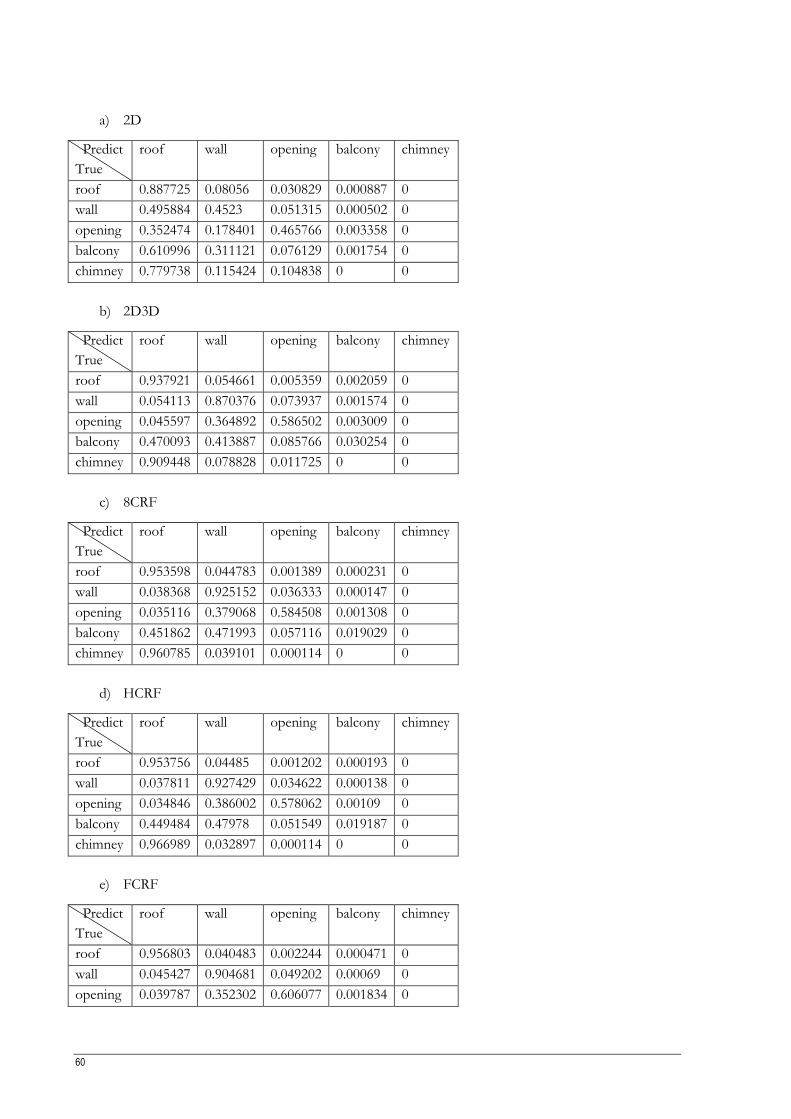
60

a) 2D

Predict

True

roof wall opening balcony chimney

roof 0.887725 0.08056 0.030829 0.000887 0

wall 0.495884 0.4523 0.051315 0.000502 0

opening 0.352474 0.178401 0.465766 0.003358 0

balcony 0.610996 0.311121 0.076129 0.001754 0

chimney 0.779738 0.115424 0.104838 0 0

b) 2D3D

Predict

True


roof 0.937921 0.054661 0.005359 0.002059 0

wall 0.054113 0.870376 0.073937 0.001574 0

opening 0.045597 0.364892 0.586502 0.003009 0

balcony 0.470093 0.413887 0.085766 0.030254 0

chimney 0.909448 0.078828 0.011725 0 0

c) 8CRF

Predict

True


roof 0.953598 0.044783 0.001389 0.000231 0

wall 0.038368 0.925152 0.036333 0.000147 0

opening 0.035116 0.379068 0.584508 0.001308 0

balcony 0.451862 0.471993 0.057116 0.019029 0

chimney 0.960785 0.039101 0.000114 0 0

d) HCRF

Predict

True


roof 0.953756 0.04485 0.001202 0.000193 0

wall 0.037811 0.927429 0.034622 0.000138 0

opening 0.034846 0.386002 0.578062 0.00109 0

balcony 0.449484 0.47978 0.051549 0.019187 0

chimney 0.966989 0.032897 0.000114 0 0

e) FCRF

Predict

True


roof 0.956803 0.040483 0.002244 0.000471 0

wall 0.045427 0.904681 0.049202 0.00069 0

opening 0.039787 0.352302 0.606077 0.001834 0

61

balcony 0.480886 0.429178 0.072853 0.017083 0

chimney 0.986454 0.013546 0 0 0

Appendix 2 Confusion matrices of 5-class show accuracy for each class (row) and each row is summed up to 1.

62

a) 2D

Predict

True


roof 0.555633 0.111388 0.107222 0.133556 0.092201

wall 0.139068 0.41558 0.176873 0.144432 0.124046

opening 0.020285 0.050763 0.636073 0.171859 0.12102

balcony 0.084365 0.154818 0.222274 0.364874 0.173669

chimney 0.026181 0.040922 0.24963 0.085487 0.59778

b) 2D3D

Predict

True


roof 0.739656 0.025792 0.007267 0.09249 0.134795

wall 0.014346 0.577627 0.243725 0.115545 0.048756

opening 0.004412 0.098602 0.76854 0.0935 0.034945

balcony 0.088373 0.093399 0.120278 0.624225 0.073726

chimney 0.063802 0.007911 0.028515 0.043369 0.856403

c) 8CRF

Predict

True


roof 0.784435 0.024237 0.003399 0.096748 0.091181

wall 0.00809 0.72994 0.159998 0.079693 0.022279

opening 0.002142 0.144776 0.764623 0.068994 0.019464

balcony 0.052015 0.109468 0.103111 0.663393 0.072013

chimney 0.084974 0.000911 0 0.00387 0.910245

d) HCRF

Predict

True


roof 0.815871 0.027672 0.00295 0.08906 0.064447

wall 0.014397 0.721781 0.165933 0.08037 0.017519

opening 0.006408 0.147281 0.762033 0.0676 0.016678

balcony 0.002145 0.107472 0.100093 0.697344 0.092946

chimney 0.353216 0.001366 0.005065 0.001195 0.639158

e) DCRF

Predict

True


roof 0.838213 0.032173 0.002929 0.073292 0.053394

wall 0.021549 0.770993 0.122916 0.069614 0.014927

opening 0.013884 0.201035 0.704349 0.066838 0.013894

63

balcony 0.08328 0.174691 0.10003 0.569109 0.07289

chimney 0.311269 0.014115 5.69E-05 0.00387 0.670689

Appendix 3 Confusion matrices of 5-class-equal show accuracy for each class (row) and each row is summed up to 1.

semantic building faÇade segmentation from … › papers_2018 › msc › gfm › lin.pdf ·...

Documents