selling money on ebay: a field study of surplus …
TRANSCRIPT

SELLING "MONEY" ON EBAY: A FIELD STUDY OF SURPLUS DIVISION
By
Alia Gizatulina and Olga Gorelkina
August 2017
COWLES FOUNDATION DISCUSSION PAPER NO. 3004
COWLES FOUNDATION FOR RESEARCH IN ECONOMICS YALE UNIVERSITY
Box 208281 New Haven, Connecticut 06520-8281
http://cowles.yale.edu/

SELLING "MONEY" ON EBAY: A FIELD STUDY OF
SURPLUS DIVISION *
Alia Gizatulina† and Olga Gorelkina‡
August 11, 2017
Abstract
We study the division of trade surplus in a natural field experiment on German eBay.Acting as a seller, we offer Amazon gift cards with face values of up to 500 Euro. Arandom selection of buyers, the subjects of our experiment, make price offers accordingto the rules of eBay. Using a novel decomposition method, we infer the offered sharesof trade surplus from the data and find that the average share proposed to the selleramounts to about 30%. Additionally, we document: (i) insignificant effects of stake size;(ii) poor use of strategically relevant public information; and (iii) differences betweenEast and West German subjects.
Keywords: Field experiment, surplus division, bargaining, Internet trade, eBay.JEL codes: C72, C93, C57.
1 Introduction
Bilateral trade is at the core of economics. Trade occurs if it generates some surplus, that is,if a buyer is willing to pay more than what a seller is willing to accept. When the buyer andthe seller bargain about the price, they bargain about the division of trade surplus.
Bargaining over the surplus division has been extensively studied in the literature, bothempirically and theoretically. Theoretical studies of bargaining take two approaches. Thefirst is the axiomatic approach, which was put forth by John Nash who looks at bargainingoutcomes that satisfy a set of desirable axioms.1 The second is the strategic approach, which
*We are grateful to Anna Petukhova for excellent research assistance. Further acknowledgements to be added.†University of St. Gallen and Max Planck Institute for Research on Collective Goods; [email protected]‡University of Liverpool Management School, Chatham Street, Liverpool L69 7ZH, UK; [email protected] central axiomatic notions are the Nash bargaining solution, the Kalai-Smorodinski solution and the
Egalitarian solution. See, e.g., Thomson (1994). When two parties bargain over money and their utilities arelinear, all three solutions imply the same outcome: the equal division of surplus.
1

focusses on equilibrium outcomes of the bargaining games. The simplest bargaining gameinvolves two players and one take-it-or-leave-it offer of one player to the second one (Güthet al., 1982). In a more complex game, players can exchange offers over several rounds, in-cluding the extreme case of an infinite-horizon bargaining game (Rubinstein, 1982). Shiftingfrom a one-round bargaining game to an infinite-horizon model leads to a drastic increase inthe first mover’s offer to the second player (Selten, 1965).2
On the empirical side, several studies have tested the ultimatum game in the lab envi-ronment. The main surprising finding in the literature is that a large proportion of openingoffers deviate from the unique subgame-perfect equilibrium of the ultimatum game, wherethe first mover takes the entire pie for himself. Instead, the observed opening offers are ratherconsistent with an infinitely repeated bargaining-game and with axiomatic solutions, wherein each case both sides get a positive share of surplus. However, given the general critiquethat is usually applied to laboratory studies, see e.g. Levitt and List (2007), the question isyet whether a non-trivial division of surplus observed in the lab is also observed in real lifebargaining situations.
The goal of our paper is to study bargaining outcomes in a natural field setting. In partic-ular, we are interested in the share of surplus that the proposing party gives to the receivingparty during the first stage of a bargaining game with at most three rounds. To conduct ourexperiment, we went to the online trading platform eBay.de and used the existing bargainingmechanism that is known as the "Buy-it-now or Best offer" selling format.3 Mimicking thetypical eBay sellers of gift cards, we collected from buyers their price offers for Amazon giftcards of different nominal values. The buyers made their offers privately (without observ-ing others’ buyers offers). We were the second movers and buyers expected that we wouldeither accept the offer, reject it, make a counter-offer or not react at all. If a buyer succeeds tobuy the card, he would typically credit its nominal value to his Amazon account and use itfor purchasing anything available on Amazon. Hence, by knowing the face values of Ama-zon gift cards, we have control over the variable which is typically unobserved, namely, thebuyer’s valuation.
On the other side of trade surplus is the seller’s outside option. From the viewpoint ofany buyer, trade surplus is the difference between his valuation and the seller’s opportunitycost. The seller’s opportunity cost is defined by the possibility to trade with other buyers orto use the card eventually on his own.4 All those are unknown to the buyer and he forms anestimate of the seller’s opportunity cost. If the buyer offers to the seller strictly more than his
2See also Binmore et al. (2007) and references therein.3This trading format should not to be confused with eBay’s second-price ascending auction, where the seller
set the starting price and bidders bid over a pre-defined period of time.4Obviously, for the market of gift cards to exist, sellers’ own valuation of the card must be less than the
nominal value of the card.
2

estimate of the seller’s outside option, he offers a non-zero share of trade surplus.
If the buyers’ estimates of the seller’s outside option were observable to us, solving forthe share of surplus that each buyer offers to the seller would be a trivial task. Obviously,we do not observe those estimates. As the result, to identify the share of surplus that a givenbuyer offers to the seller we have to infer the buyer’s belief about the seller’s opportunitycost.
We developed a new statistical method to use our own data to infer the subjects’ beliefs.In our model those beliefs could be any, i.e., we do not impose the requirements of consis-tency with the publicly observed data or any kind of rationality or a common prior. As eachobserved offer is a non-degenerate function of two variables, it is not feasible to decomposethe offers at the level of individual observations. However, under our model’s assumptions,which we discuss below, we can implement an aggregate decomposition program, where theobserved distribution of offers is decomposed into a distribution of shares of surplus and adistribution of the buyers’ beliefs about the seller’s expected opportunity cost.
In our setting, to decompose the observed distribution of normalized offers in two un-derlying unobserved distributions we have to solve an integral equation with two unknownfunctions. This problem is infinite-dimensional and computationally hard. To obtain a feasi-ble program, we first reduce the dimensionality. For this, in line with the standard approxi-mation theory, we restrict the set of possible distributions to be a family of finite polynomials.Our search for fitting distribution starts with the uniform law as a candidate solution for bothfunctions. We consecutively raise the polynomial degree until the optimal solution passes apre-specified goodness-of-fit test. To check the robustness of the main method’s findings, wealso apply two further estimation methods, including a non-parametric one.
Our key finding is the following distribution of shares of surplus that buyers offer to theseller:
Share of surplus: 0-10% 10-20% 20-30% 30-40% 40-50%
Percentage of subjectsoffering the share : 33.2 3.7 3.6 16.6 43.0
Table 1: Estimated distribution of surplus shares offered by eBay users.
By the very nature of our estimation method, this distribution of shares is free from anyeffects of competition among buyers or any other origins of buyers’ beliefs about the seller’soutside option. Hence, it can be compared to the findings from experiments on a one-shortbilateral bargaining model, i.e., the ultimatum game.
As one can see, approximately 43% of subjects offer 40-50 % of trade surplus to thecounter-party. This implies that even in a large anonymous market like eBay, equal splitting
3

of the total trade surplus is rather usual. Whether the equal split is due to social preferences,cultural norms, its salience, simplicity, or the axiomatic properties of the egalitarian solution,our results imply that its occurrence in the field is similar to that in the lab. On the otherside, about one third of all subjects have behaviour consistent with the maximization of in-dividual monetary payoffs, offering no more than 10 % of the trade surplus. The averageshare offered is 29.4 %, which falls within the range of estimates typically obtained in labexperiments of the ultimatum game (e.g., Oosterbeek et al., 2004).
Our estimation technique rests on three assumptions. First, the card is worth its nominalvalue to any buyer who makes a sizeable offer in the experiment. The money on the Amazonaccount, can indeed be split, stored, combined with other payment methods and used forpurchasing goods from both Amazon and third-party sellers that operate on the platform. Toan Amazon customer, the money on his Amazon account is thus no different from the moneyon a credit card.5 If, however, the cards are worth less than their nominal value to somebuyers then our results imply that the sharing is even more generous than our estimatessuggest. More precisely, the estimated distribution is first-order stochastically dominated bythe true one. In that sense, we have obtained a lower bound on the sharing intentions (seealso Section 5.1). Moreover, we do not need to assume that the subjects who make extremelylow offers fully appreciate the card’s value.
Second, we assume buyers’ risk-neutrality. In the lab studies of bargaining, this assump-tion is standard. Moreover, our data suggests that the subjects are risk-neutral within therelevant range of payoffs. This is shown by contradiction. If the subjects were risk-averse inthis range, we would have observed that the distribution of offers changed as we increasedthe stake. This, however, is not the case in our data (see Section 5.2).
The third assumption postulates that subjects’ beliefs and sharing intentions are statis-tically independent. This follows from the predominant economic approach to rationality,which implies maximization of utility given subjective beliefs. Fundamentally, utility for-malizes preferences over allocations and the belief function reflects the knowledge about thegame. We similarly regard sharing intentions as an expression of subjects’ preferences whiletheir beliefs are formed through their information and individual experiences from the game.
Regardless of all of the above assumptions we obtained a number of further results fromthe regression analysis. First, as noted above, we find that the observed distributions ofnormalized offers6 do not vary with the amount of money at stake. Second, we find that ob-served buyer behaviour is insensitive to public information about the degree of competition,
5On the other hand, the gift cards are not worth their face value to those selling them, or generally non-customers of Amazon. EBay customer protection service guarantees that the buyer gets all goods as described;seller fraud is therefore not a determinant of the card’s value.
6A normalized offer is a price offer divided by the card’s face value. For example, the value of a normalizedoffer that corresponds to 40 Euro for a 50-Euro gift card is 0.8.
4

as well as to the public history of sellers’ responses to price offers. Third, we use data onbuyers’ postal codes to classify the subjects in two regions, East and West Germany. Whileboth groups of offers tend to cluster at 50% of the card’s value, the "naïve equal split" is moreprevalent among subjects in East Germany.7 Thereby, West German subjects are more likelyto make competitive offers, that is, to be consistent with the theoretical prediction of a modelwith multiple buyers.
The present study is the first bargaining experiment to include a non-standard (non-student) subject pool and to feature a field context in which the subjects undertake the tasknaturally. Moreover, the subjects did not know that they were participating in an experi-ment.8 Therefore, our experiment is a natural field experiment, according to the definitionof Harrison and List (2004).
The next section describes the experiment and its data. The decomposition strategy andits results are presented in Section 3; robustness checks are described in Appendix A.4. Sec-tion 4 reports on the regression analysis. Section 5 discusses the assumptions and the relatedliterature. Section 6 concludes.
2 Experiment
2.1 Amazon Gift Cards
We set up a controlled environment within an existing secondary market for Amazon giftcards on the German site of eBay (www.ebay.de). Amazon gift cards are used primarily aspresents.9 Typically, the gift giver would go to the Amazon website, pay V Euros to get asixteen-digit code, and transmit the code to the gift receiver. Subsequently, the receiver logsin to his Amazon account, enters the code and gets V Euros credited to his account. Theaccount credit can be used for purchasing any goods offered on the Amazon website,10 it canbe split, combined with other payment methods and stored for up to three years.
If the gift card owner does not intend to use the code, he puts it up for sale in a secondarymarket. Upon purchase, the code is transmitted in a secure message. In Germany, resellingAmazon gift cards on eBay is very common. For instance, 87 gift cards were on sale at 7p.m. on June 13, 2014, and 1962 sales in total were posted within 114 days prior to that date.
7A 50% offer can be viewed as an equal split of trade surplus only under a "naïve" assumption that theseller’s outside option is 0.
8The fact that we work with unaware eBay users is the distinction of our setup from Bolton and Ockenfels(2014).
9Other uses include: reward for participation in internet surveys, including lottery prices, payment forconsumer-to-consumer online purchases, bonus to third-party promotions.
10The goods can be bought from Amazon.com, Inc. / Amazon EU S.a.r.l. as well as any other seller, privateor institutional, that uses Amazon as platform.
5

Nominal values of gift cards ranged from 5 to 2500 Euro.11 The market turnover in Q4 2015is estimated at 70 000 Euro.
2.2 The "Buy-it-now or Best Offer" format on Ebay
In the experiment, we employ the Buy-it-Now or Best Offer (BINBO) format of eBay, So-fortverkauf oder Preisvorschlag in German. The BINBO sales format is an alternative to thebetter-known eBay auction, which is an English auction where the bidders openly competewith each other.
The rules of BINBO are as follows. Initially, the seller posts an ask price and invites thebuyers to either pay the ask price or make their own price offer. When a buyer makes anoffer, the seller has forty-eight hours (or less, if the listing expires earlier) to accept, reject, ormake a counter-offer. When a price offer is accepted, the card is sold and the game ends. Alisting becomes inactive if it expires or if the card is sold to a buyer. EBay users can browsethe history of inactive listings.
Figure 1: BINBO.
The BINBO game is illustrated in Figure 1.The card value is normalized to 1. The buyer’soffer is denoted bi, where i refers to a buyer-sellerpair. When bi is below the ask price, the selleraccepts or rejects; no reply is strategically equiv-alent to a rejection. If the seller accepts he getsbi, if he rejects he saves the opportunity cost oftrade ci. The seller’s cost of trade ci is due to theopportunity to trade with other buyers and thecard’s usage value to the seller. The buyer gets1− bi in case of acceptance and zero in case of re-jection. If the buyer accepts the seller’s ask price,bi equals the ask price and the seller is bound toaccept, i.e., to transfer the card code. When an of-fer bi is accepted, the surplus 1− ci is effectivelysplit between the buyer who gets 1− bi and theseller who "gets" bi − ci. Note that Figure 1 omitsthe possibility of counter-offers; their role is dis-cussed in Section 5.4.
11One may wonder that such expensive goods could be sold anonymously over the Internet. This is due, to alarge extent, to efficient consumer protection services offered by eBay, as well as the importance of reputation (seeResnick et al. (2006)). Note also that Germany ranks high on the level of trust between strangers (see Fukuyama(1995)). On the relation between culture and e-commerce diffusion see Gibbs et al. (2003).
6

When an eBay user makes a price offer he becomes a subject of our study. The subject(buyer) observes the posted price and the following information. First, he can observe thetotal number of offers received by the seller: 0, 1, 2, etc., the timing and the status of eachoffer: pending, rejected, counter-offer received. Second, the buyer observes the number ofminutes left before the listing expires, the seller’s feedback score, and the other items theseller currently offers for sale. The buyers can also observe the history of previously offereditems of this seller. The most immediate information about the seller’s history is the list ofall feedback entries (positive, negative, neutral) that are left to the seller for the items that hehas sold.
Importantly, only the seller can see how much money is being offered. The buyers canonly observe how many competitors are present, if at all.12 Naturally, no-one observes howmany competitors there will have arrived until the listing expires, as that information per-tains to the future.
2.3 Listings
We offer Amazon gift cards with a range of face values: 5, 10, 20, 50, 100, 200, and 500Euro, i.e., in total seven treatments. In two waves of the experiment, March to July 2014 andMarch 2015, we posted over 200 listings. Each listing lasts three days, the lowest possibleduration on eBay. We used five different seller accounts with feedback scores ranging fromno feedback and no tenure to 430 stars and 10 years tenure. Each seller account listed oneor two gift cards at a time, and the nominal values of the gift cards rotated between selleraccounts over the entire duration of the experiment.
The text of the announcement and the video illustration URL are given in Appendix A.1.
We drafted the listings in a way that mimics the common practice of the gift card salesvia the BINBO format. Relying on the history of similar posts, we used typical wording andset the initial ask prices above the nominal value of the gift card13. On top of replicating thecommon practice, the excessive ask price allowed us to limit the number of actually executedtransactions: rational buyers should not accept to pay more than the card’s nominal value.To our surprise, the excessive ask price was accepted on a few occasions. The explanation ofoverbidding is the focus of Malmendier and Lee (2011). As for this paper, we concentrate onoffers that do not imply a loss. Finally, to unify the sellers’ response to offers, we let all offersto expire without any our response.
12Similarly, in Camerer (2003) and Roth et al. (1991), the proposers do not observe their competitors’ offers.13E.g., we set the ask price of a 100 Euro gift card equal to 119 Euros
7

2.4 An Illustration
As an illustration, consider one round of the experiment. We list a gift card with the nominalvalue of 100 Euro on June 1 at 1:08 p.m. We receive the first offer of 90 Euro from the buyerhaving the user name “lu..er” and who has 6 eBay feedbacks as of June 3 10:16 a.m. and thesecond offer of 80 Euros from the buyer “xx...30” with 60 feedbacks at 1:23 p.m.
At the moment “lu..er” placed his offer, he could observe that there were no offers out-standing. In contrast, the second buyer “xx...30” could see that he was facing competitionfrom one other buyer.
We let both offers expire on June 4 at 1:08 p.m. This generated two observations. Thedata collected per observation include the offered amount, the exact timing and order of theoffer, the buyer characteristics (eBay alias, feedback score and registered postal code), as wellas the seller’s information and the exact time the listing was posted. We also keep track ofthe announcements that did not receive any offers.
2.5 Data
Figure 2: Cumulative distribution functions of the observed(blue), and uniform (red) arrival times, normalized to one.
72 percent of the listings receive at least oneoffer within the three-day period. The num-ber of offers per listing ranges from 0 to 15,with 1.6 offers made on average. One offerper listing is both the median and the mostfrequent number of offers, and correspondsto the situation of bilateral trade.
The subjects come from all over thecountry, 15 percent of the offers originate inEast Germany (former German DemocraticRepublic).14 The most experienced buyer inthe sample was registered on eBay 16 yearsprior to our experiment. On average, buyershad 8.5 years of eBay experience.
The distribution of the arrival times ofprice offers within the duration of sale isplotted in Figure 2. The diagonal corresponds to the uniform distribution. The times arenormalized to one according to the formula toffer−tlisting
3×24×60 , where t is expressed in minutes. Con-trary to the case of eBay’s ascending auction, where the bidding frequencies spike at the
14Five offers from Austria were not included in either East- or West-German group.
8

end of sale (see, e.g., Roth and Ockenfels (2002)), we do not observe any such patterns inthe arrival rates in the BINBO format we use in the experiment. This is not surprising sincewaiting to place an offer is not profitable in a BINBO sale.
Voucher Value All 5 e 10 e 20 e 50 e 100 e 200 e 500 e
No. of Listings 221 46 25 19 22 36 43 30No. of Offers 358 42 45 38 57 60 74 43Average Bid 0.73 0.71 0.77 0.73 0.77 0.70 0.72 0.71
Std. Err. 0.04 0.11 0.11 0.12 0.10 0.09 0.08 0.11Std. Dev. 0.23 0.23 0.18 0.17 0.17 0.27 0.23 0.29Median 0.80 0.80 0.80 0.75 0.80 0.80 0.79 0.82
Table 2: Descriptive statistics of normalized offers bi = Bi/Vi, "Offer / Nominal Value".
The offers in our sample range from 1 Euro, the lowest admissible offer on eBay, to thenominal value of the gift card. To make the data comparable across treatments, we normalizethe offers by dividing each offer by the nominal value of the gift card. The pooled datadisplay clustering: the normalized offers concentrate around 0, 50, 80, and 90 percent of thegift card value (see Figure 4).
The descriptive statistics, broken down with respect to nominal value treatments, arereported in Table 2. Overall, the distribution of offers is right-skewed: every second offerexceeds 80 percent of the nominal value. The average offer in our sample ranges from 71 to77 percent of the nominal value and does not display monotonicity with respect to the giftcard’s nominal value. The same is true of median values that range from 75 to 82 percent ofthe nominal value.
Figure 3: Gift card nominal values along the horizontal axisin log scale. Normalized offers, mean, standard error bandalong the vertical axis.
Figure 3 presents the data, where thelogarithm of the nominal card value is plot-ted against the horizontal axis and the nor-malized offer is the dependent variable onthe vertical axis. We use the one-wayANOVA to test whether the empirical av-erages vary across the nominal value treat-ments. We find the null hypothesis of equalmeans is not rejected,15 implying the nor-malized offers’ invariance in scale. Pair-wise linear and log-linear regressions yielda similar finding: the nominal value doesnot have a statistically significant effect on
the normalized price offers (see Table 5).Overall, our analysis indicates that stake size does
15ANOVA P-value = 0.50.
9

not affect the normalized offers in the population of eBay buyers. Similar findings wereobtained in the lab settings by Cameron (1999), Munier and Zaharia (2002), Hoffman et al.(1996), Slonim and Roth (1998).16
3 Decomposition of Offers
In this section we study the sharing intentions behind the subjects’ offers in the experiment.Figure 4 is a histogram that presents the data pooled across value treatments.
Figure 4: Empirical frequency h(bi) of normalized offers bi = Bi/Vi. The relative offers bi are grouped into five-percentbins and plotted against the horizontal axis. The bins include the upper bound of the interval, for instance, the last bincorresponds to bi ∈ (0.95,1].
The experimental data displays substantial heterogeneity and irregular clustering: in par-ticular, we observe clusters at around 0, 50 and between 80-90 percent of the card’s nominalvalue. An offer of 50%, where we observe a spike in frequency, would correspond to an equalsplitting of surplus, if the seller’s outside option (cost) was zero. Similarly, the seller couldonly accept an offer close to zero, if zero was his cost. In reality the seller’s cost of trade isdifferent from zero; this also appears to be the belief of the majority of subjects, who offer theseller 80% of the card’s value or more.
16A meta-study by Oosterbeek et al. (2004) documents a small negative effect of increasing stake size. Slonimand Roth (1998) and Roth and Erev (1995) find a positive effect when the game is played in the first round oronly played once.
10

Overall, the observed pattern of offers points at stark heterogeneity in the subjects’ per-ceptions of the game and (or) their intentions when playing it. Therefore, our treatmentof the data does not impose any structure on the subjects’ beliefs about the seller’s outsideoption, in particular, we do not assume a common prior.
3.1 The Decomposition Problem (DP)
Our model allows for subject heterogeneity across two dimensions: the perceptions of theseller’s outside option (seller’s cost) and the sharing motives. The perception of the seller’scost c is subject to uncertainty of the number of competing bids and of their sizes, as well asthe seller’s own usage value of the card, if any. In our model, the buyer’s perceptions of care captured by a distribution function Φi(c) that we refer to as the buyer i’s belief over c.17
The buyers’ beliefs are thus the first source of offers heterogeneity.
The second source of the observed subject heterogeneity is the sharing motive, or thefraction of surplus that a subject offers in excess of the seller’s cost. Consider first a fixedseller cost c. The surplus from trade is given by 1− c, the difference between the buyer’svalue and the seller’s cost. In the game of bargaining over the surplus 1− c the buyer’s priceoffer implies how the surplus is split. Buyer i’s price offer bi leaves the seller with a sharesi of surplus: si =
bi−c1−c , where c is the seller’s true cost. For a fixed c, the price offer bi(c) is
therefore given bybi(c) = c + si (1− c) . (1)
However, since c is uncertain, the offer is
bi =
ˆbi(c)dΦi(c) =
ˆ[c + si (1− c)]dΦi(c)
= ci + si (1− ci) , (2)
where ci ≡´
cdΦi(c). The observed offer bi is the solution of the bargaining problem in buyeri’s subjective expectation over the seller’s cost c. Note that (2) implies that the first moment ci
of Φi(c) is sufficient information to calculate the buyer’s offer when si is known.
Equation (2) summarizes two sources of variation in offers that we observe. First, thesubjects vary in the normalized shares si they are willing to offer to the seller. Second, theydiffer in their expectations ci of the seller’s opportunity cost c. To understand the prevalenceof sharing rules in the data, we have to extract si from the observed normalized offers bi.
17Formally, c = max{
us,max{
bj : j ∈ J}}
where us is the seller’s own usage value, and J is the set of com-petitors, bj is the bid of competitor j.
11

Clearly ci and si cannot be identified from an observed offer bi. Since the observed offer isa function of two unknowns, decomposing bi is infeasible at the level of individual observa-tions. However, one can implement an aggregate decomposition of the observed distributionof normalized offers into a distribution of shares si and a distribution of the first moments ofthe belief functions ci. The aggregate decomposition implies splitting of the observed distri-bution of offers into a distribution of shares si and a distribution of subjective expectations(first moments of the belief functions) ci. The aggregate decomposition is a novel statisticalapproach to analyse of partially controlled experiments. We drop the subscript i in whatfollows.
To formally specify the Decomposition Problem (DP), we let f (s) and g (c) denote, re-spectively, the unobserved distributions of the shares s and of the cost expectations (belieffirst moments) c. Let h (b) be the observed distribution of offers. Capitals F, G, and H denotethe corresponding cumulative distribution functions. For simplicity we think of all threedistributions as having continuous supports. We assume that the supp(g) = [0,1], supp( f ) =[0,0.5], where the 0.5 bound follows from the standard other-regarding preference theories.18
We demonstrate the robustness of the results by relaxing this bound in the Appendix Table15. Note that “selfish” offers (maximizing individual payoffs given subjective beliefs) corre-spond to si = 0 for all i and are therefore allowed in this specification.
Assuming that offered shares and cost expectations are distributed independently in thepopulation, the distributions are related through the following equations:
H (b) = Pr (c + s (1− c) < b) = Pr(
c < b, s <b− c1− c
)=
ˆ b
0
[ˆ b−c1−c
0f (s)ds
]g (c)dc =
ˆ b
0F(
b− c1− c
)g (c)dc. (3)
The cumulative distribution function H on the left-hand side is given by the observations inour experiment. The right-hand side integrates over all c and s that generate an offer less orequal to b, according to (2). The essence of the decomposition problem (DP) is to find f (s)and g (c) that best fit equation (3) given H(b) constructed from the experimental data.
3.2 Computational Issues and Uniqueness
Decomposing the observed distribution of normalized offers into two underlying unob-served distributions is equivalent to solving an integral equation with two unknown func-tions. As both f (.) and g(.) belong each to an infinite-dimensional space, the DP (3) isinfinite-dimensional and, therefore, computationally hard. Finding a solution calls for a
18See, e.g., Fehr and Schmidt (1999) [Proposition 1], Ockenfels and Bolton (2000) [Statement 3].
12

reduction in the problem’s dimensionality to a point where optimization becomes computa-tionally feasible. What complicates the analysis further is that while the solution to (3) existsit may not be unique unless the space of functions f (.) and g(.) is restricted.19
Our approach to solving the DP (3) addresses both issues, the dimensionality reductionand uniqueness. We run three alternative optimization programs to cross-check the findings.Two programs are parametric; dimensionality reduction is achieved by restricting the solu-tion to a space of parametric functions. The first, baseline program is reported in the next sec-tion 3.3. It relies on the standard approximation theory and looks for a solution in the spaceof polynomials. The second program, reported in the Appendix A.4.1 is non-parametric. Thedimensionality of the DP (3) is reduced by discretizing the supports of f and g. Finally, inthe Appendix A.4.2 we restrict f and g to the class of beta functions, which permits a globalsearch for four parameter estimates (two for each distribution). All three programs yieldsimilar results, however the beta approximation is rejected by the goodness-of-fit test.
In the following section we focus on the polynomial program and report its results inTable 3.
3.3 Polynomial Approximation
Our baseline program achieves the reduction of dimensionality by restricting the solution toa set of continuous functions, in particular, to a space of parametric functions. Following thestandard approximation theory, the space of finite polynomials is the best choice within aparametric class.20 Hence, our goal is to identify a polynomial approximation of H. Conse-quently, we treat both f and g as linear combinations of Chebyshev polynomials:
fn (s;γ) =n
∑k=0
γkTk (s) , 0≤ s ≤ 0.5, (4)
gm(c;δ) =m
∑i=0
δkTk (c) , 0≤ c ≤ 1, (5)
where Tk(x) is a k-degree Chebyshev polynomial of the first kind.
19There always exists a trivial corner solution, where h≡ g and f is a Dirac delta function with the entire prob-ability mass concentrated at zero. Sadovnichy (1986) shows that, for a given kernel function F(b, c), a Volterraintegral equation such as (3) is a contraction mapping and hence has a unique solution g∗. Since both f and g arerestricted to the class of probability measures, Sadovnichy’s result does not imply that one can generate multiplesolutions by simply varying the kernel function.
20By the Stone-Weierstrass theorem, the subset of polynomials is dense in C[a,b] which means that any con-tinuous function on a bounded interval can be approximated arbitrarily well by a sufficiently large degree poly-nomial.
13

The iterative procedure starts at n = m = 0. That is, the initial candidate solution forf p = f0 and gp = g0 is a pair of zero-degree polynomials, which corresponds to two uni-form distributions. Subsequently, we raise the polynomial degree until the optimal solutionwithin the respective class passes a goodness-of-fit test.
More specifically, at each iteration we search for the vector of parameters (γ,δ) that min-imizes the Kolmogorov-Smirnov distance between H and H
(γ∗n,δ∗m) = argmin(γ,δ)
dKS (Hnm(·;γ,δ), H(·)) (6)
subject to´ 0−∞ fn (s;γ)ds= 0,
´ +∞0.5 fn (s;γ) = 0, fn (s;γ)≥ 0;
´ 0−∞ gn (c;δ)dc= 0,
´ +∞1 gn (c;δ)dc=
0, gn (c;δ) ≥ 0, where the Kolmogorov-Smirnov distance is
dKS(
H(·), H(·))= supb∈[0,1]
∣∣H (b)− H (b)∣∣ , (7)
and Hnm is a composition of
Hnm (b;γ,δ) =ˆ b
0
ˆ b−c1−c
0fn (s;γ) gm (c;δ)dsdc. (8)
Once we find the best approximations ( fn(·;γ∗n), gm(·;δ∗m)) for fixed polynomial degrees nand m, we take the respective composition H(·;γ∗n,δ∗n), and compare it to the observed cu-mulative distribution H(·). We dismiss the solution if the respective Kolmogorov-Smirnovdistance between H(·;γ,δ) and H(·) exceeds the bootstrapped critical value and proceed tothe next iteration allowing for an extra polynomial term.21
At n = 3, m = 4 the hypothesis that H = H is no longer rejected. In other words H(·) isstatistically indistinguishable from the empirical H(·). To avoid overfitting we terminate theprocedure at this iteration and adopt the respective solution
(f p(·), gp(·)
)= ( f3(·;γ∗4), g4(·;δ∗4 )).
As a robustness check, the procedure was reiterated with higher polynomial degrees up toten; this did not improve the distance significantly and each subsequent solution was qual-itatively similar to
(f p(·), gp(·)
). In summary, the estimated
(f p(·), gp(·)
)is stable, data-
consistent, and uniquely optimal polynomial approximation.
Remark We used Mathematica’s differential evolution fitting method, allowing for 500 iterationsat each round of search. The advantage of the differential evolution method is that it consistent atfinding the global solution. The search procedure requires that a continuous version of H is generated.To that end, we derive a non-parametric kernel density function from the data, setting the bandwidth
21Bootstrap critical values corresponding to 358 observations are 0.049 for significance at 10%, 0.057 for sig-nificance at 5%, and 0.071 for significance at 1%.
14

at 0.015. This value allows for the used H to be sufficiently continuous while still preserving theinformation contained in the empirically observed version of H.
3.4 Results of Polynomial Decomposition
The estimated distributions are presented in Table 3. (The corresponding Chebyshev coef-ficient estimates are given in the Appendix, Table 11.) The estimate of the distribution ofsharing rules f implies that 43− 44% of the subjects offer 40 to 50% of the trade surplus tothe seller. One third of all our subjects make "greedy" offers and propose no more than 10 %of the trade surplus to the seller. The remaining 25− 30% of the subjects make offers between10 and 40%. The average offer to the seller amounts to 29.4% of the respective trade surplus.
s: 0-10% 10-20% 20-30% 30-40% 40-50%f p (s): 33.2 3.7 3.6 16.6 43.0
c: 0-10% 10-50% 50-60% 60-70% 70-80% 80-90% 90-100%gp (c): 11.2 10.1 11.8 17.7 21.1 19.2 8.9
Table 3: Estimated distributions of sharing rules f p (s) and cost expectations gp (c) in the population of eBay buyers (inpercentage points). dKS = 0.028.
The estimated g(.) evokes of a mixture of two distributions. (See also Figure 5 that reportsthe quantitatively similar non-parametric estimates.) This suggests that there are two typesof beliefs that prevail in the population of bidders. There is a fraction of "naïve" subjects,estimated at 11− 14%, who make their offers under the assumption that the seller’s outsideoption (cost) is null. The first moments of the beliefs of the remaining "sophisticated" major-ity of the subjects are described by a bell curve centered around the observed average offerof 73%. This suggests a certain "crowd wisdom" manifests itself in the eBay market of Ama-zon gift cards – the expectations of seller’s cost are correct, on average, in the "sophisticated"group of subjects, even though there is noise around the value.
3.5 Robustness Checks
To verify whether the decomposition we found is robust, we have conducted further decom-positions, using two alternative approaches. One approach, reported in Appendix (A.4.1), isto discretize the support of distributions h, f , and g, in order to obtain a finite-dimensionalproblem. Namely, we partition the support of the three distributions into equal-sized bins.Given the upper limit on the support of sharing rules of 50% and a bin size of 10%, we obtaina substantially simplified problem with fifteen unknowns. We use an iterative numerical op-timization to assign a probability mass to each of the bins. This program yields distribution
15

functions similar to the baseline solution. The average offered share of surplus (the mean ofthe estimated f np) amounts to 29.8% according to the non-parametric estimates. See Figure5.
Figure 5: Estimated distributions of sharing rules f np (s) and cost expectations gnp (c) in the population of eBay buyers(in percentage points). dKS = 0.0077.
Our second robustness check, reported on in the Appendix A.4.2, employs a differentparametric program that restricts both f and g to the class of Beta probability distribu-tions. The restriction to the Beta class boils the problem down to only four unknowns (eachbeta distribution is described by two parameters). While the resulting fit measured by theKolmogorov-Smirnov distance is unsatisfactory, the similarity of the beta functions solutionto our main result suggests that the findings are robust.
4 Regression Analysis
The regression analysis is a separate exercise that we conducted on the raw data. The maintake-away from this section is to confirm that the offers cannot be explained by the observ-able characteristics. It therefore suggests that the decomposition approach is necessary toaccount for heterogeneity.
By the design of the experiment, we know exactly what information was available to thebuyer at the time he made his offer, as well as several characteristics of the buyer himself.The dependent variable in all regressions is the normalized offer bi.
4.1 Competition Marks
We start by looking at the effects of information about the number of competitors for a giftcard. In BINBO, the buyers observe two signals informative of competition intensity. The
16

first signal is the amount of time remaining before the listing expires: the more time is left,the more buyers are expected to arrive by the end of sale, and the higher is the degree ofcompetition. The second signal is the number of offers already outstanding by the time agiven buyer makes his offer; naturally this signal conveys the information in a more directway. Both indicators are displayed next to the ask price and barely involve any search effort(see the screen-cast URL p. 24). Both indicators should make buyers update their beliefsabout the seller’s outside option. This, in turn, should have an effect on the buyers’ normal-ized offers. However the regression results demonstrate that both signals have insignificanteffects on the subjects’ normalized offers (see Table 5 in the Appendix).
We take a further step to verify whether the simplest binary indicator of competition pro-duces an effect. Specifically, we split the offers in two groups: those arriving first on a listingand those arriving when at least one other has been already made. The respective empiri-cal distributions are presented in Figure 7 in the Appendix. Again, we find no significantdifference in both groups’ mean offers.22
Beside the obvious explanation that any updating, however simple, is inhibited by cog-nitive costs, we offer two alternative reasons why the competition marks fail to produce anysignificant effects in the experiment. First, the subjects may use a rule of thumb when mak-ing offers, drawing on their past experience of gift card sales. Such an approach is aimed ata longer-term market performance and substantiated by a large bulk of psychological liter-ature, e.g., Tversky and Kahneman (1974), Newell et al. (1972), Gigerenzer (2007). Second,the buyers may (rationally) expect that if the gift cards remain unsold by the deadline theygo on sale again in the future. Therefore, the expected stream of future offers may outweighany present competition, making the latter effect statistically insignificant.
4.2 Subjects’ Learning
Next, we test whether the normalized offers change over the course of our experiment, whichmay occur due to subjects learning about the environment. The subjects get informationabout the seller’s response strategy from two sources. First, the history of sales was avail-able through eBay’s search engine at the time we conducted the experiment. For all fiveaccounts used in the experiment, browsing the history of the account revealed that a num-ber gift cards were listed exclusively in BINBO format and remained unsold.23 While thisinformation could have stopped some buyers from making an offer, the regression analysissuggests that the size of normalized offers was unaffected by history (see Tables 6 and 7 inthe Appendix). To proxy the opportunity of learning from history, we use calendar time:
22ANOVA P-value = 0.13.23Apart from a few cases when we received offers to pay the posted price that exceeds the card’s value.
17

subjects participating at the start of the experiment have less evidence on our response be-haviour than those arriving toward the end of the experiment. This finding implies that thesubjects did not browse sale histories or did not take the information into account.
Second, buyers can learn from their own experiences of making an offer to a particularseller. To study the possible effect, we look at the sub-sample of the recurrent buyers. Intotal, 56 out of 277 buyers in our experiment made offers on multiple listings. We trackhow those buyers’ offers change over time. Specifically, we calculate the increment of eachsubsequent offer relative to the previous offer that buyer made. This variable captures thesubject’s learning dynamics due to his or her experience with one of the seller accounts weuse. Student’s test finds no statistically significant change in offers between two consecutiverounds of a subject’s participation.24
4.3 Effects of Experience
Buyers’ eBay experience, reflected by their feedback score,25 has a mild positive effect onnormalized offer sizes (significance at 10%; see Tables 6, 7, 8 and 9 in the Appendix). Even ifthe effect is present, its size is extremely small. For instance, an inexperienced buyer with nofeedback offers 1 percentage point less than the average buyer with 450 feedback entries.
A similarly sized effect, also statistically significant, is produced by the increase of theseller’s feedback score. However, while the effect of buyer experience is linear, the marginaleffect of the seller’s experience decreases. Specifically, the effect on the normalized offer ofextra feedback that the seller receives decreases drastically after just 12 feedback entries.26
The effects of buyer and seller experience do not display complementarity, i.e., there is noevidence that more experienced buyers make significantly higher or lower offers to moreexperienced sellers.
4.4 East and West Germany
Using data about buyers’ registered postal codes, we identify the impact of each subject’slocation on the size of the offer. Our sample contains about 15% of offers stemming fromthe states on the former GDR territory.27 Our main observation here is that when subjectsare grouped by region, there are important differences in the distribution of offers between
24P-value = 0.317.25Note this is an imperfect measure of experience, due to the benevolent nature of ratings. In particular, the
sellers’ incentives to leave feedback are limited, since they can only leave positive feedback.26There is a statistically significant effect of seller experience when we use the feedback score from 5 accounts
jointly (P-value is equal to 1.9× 10⁻⁴). Splitting the sample into two groups, for sellers with zero feedback andat least 12 feedback entries results in P-value of 0.79 and 0.68, respectively.
27Postal codes are only indicative of current residency, not the subject’s origin.
18

East and West Germany. In the latter group, we observe a larger number of offers that areclose to the competitive prediction – near 95 percent of the gift card value. By contrast, thebuyers from East Germany make more offers in a close neighbourhood of 50 percent of thetotal value. (See Fig. 6 in the Appendix).
Can this variety in offers be attributed to the remaining cultural differences between Eastand West Germany? From the previous analysis we know that a buyer’s experience affectsthe average size of his offer to the seller: more experienced buyers tend to make slightlyhigher offers. Since West German buyers in our sample have more experience with eBay,the regional difference we observe may be due to the difference in experience. In order tocorrect for the possible bias, we extract a sub-sample of buyers from West Germany that hasthe same the distribution of feedback scores as the East German sample. After the correction,the distributions of normalized offers remain virtually unchanged and the same differencepatterns emerge. The equal split of the "naive surplus" is a significantly more important focalpoint for East German subjects, while the competitive offers are more common among theWest German subjects. In the next section, we also report on the difference between tworegions at the level of offered shares of surplus.
For instance, in a large scale empirical study Alesina and Fuchs-Schuendeln (2005) foundthat East Germans displayed higher preference for equality and redistribution – somethingthat could reinforce the prevalence of equal splits. In two waves of a public good experiment,Ockenfels and Weimann (1999) and Brosig-Koch et al. (2011) find important differences inEast and West German behaviour, which persisted two decades past the reunification. Focus-ing on children and adolescents aged 10 to 18, John and Thomsen (2013) find more supportfor other-regarding preferences in East than in West Germany.
5 Discussion
5.1 Subjects’ valuations
Suppose that the subjects do not always value the cards at their full nominal value. In thatcase the distribution of bids is given by:
H (b) =
ˆ b
0
[ˆ 1
bF(
b− cv− c
)dW (v |v > b )
]g (c)dc, (9)
where dW (v |v > b ) is the conditional distribution of the subject’s true valuation v. Thevaluation of a rational subject cannot be lower than his bid b, but it cannot exceed 1 sincethe gift card can be bought at the price of 1 on the Amazon website. Comparing the original
19

problem with (9) we observe that our reported estimate F is in this case is equivalent to theexpectation of F over the values v:
F(
b− c1− c
)≡ˆ 1
bF(
b− cv− c
)dW (v |v > b ) . (10)
Since function F is a c.d.f. and increasing, we obtain the inequality:
F(
b− c1− c
)=
ˆ 1
bF(
b− cv− c
)dW (v |v > b )
≥ˆ 1
bF(
b− c1− c
)dW (v |v > b ) = F
(b− c1− c
). (11)
Inequality (11) implies that our estimate F is first-order stochastically dominated by F. There-fore, if the subjects’ valuations are less that the card’s value then our estimate of sharing rulesprovides a lower bound on the actual sharing.
One may argue that the subjects offering, for instance, 1 Euro for a 100 card value the cardlower than 100 and simply "try their luck". This is to a large extent inconsequential to ourestimates. To continue with the example, as long as the subject’s true value V < 100 is above10 Euros his offer of 1 Euro will be allocated to the lowest 10% bin anyway (i.e., he still offersbetween 0 and 10 percent of V). Therefore the results of the non-parametric decompositionwill not change. If however the subject’s value for a 100 Euro card is less than 10 Euros thenwe are back to the lower bound.
5.2 Risk-neutrality assumption
We have assumed that our buyers are risk-neutral. This assumption is supported by ourown data and by the size of the stakes that we used. But it is also confirmed by the existentliterature. In particular, given the empirical evidence for an increased risk aversion at highermonetary stakes (see, e.g., Holt and Laury (2002) and references therein), if buyers wererisk-averse we would observe a reduction, on average, of offers for the gift cards of a highnominal value, e.g. 200 or 500 Euro.28 The regression results do not support this hypothesis(see Tables 5-10 in Appendix). Similarly, Fehr-Duda et al. (2010) demonstrate that the riskaversion is not identifiable in the data when the stakes are comparable to ours.
28In 2014, the monthly disposable median net income per capita in Germany amounted to 1644Euro (European Commission data: http://ec.europa.eu/eurostat/web/gdp-and-beyond/quality-of-life/median-income)
20

5.3 Competition with other sellers
As the sellers of gift cards, we face competition from other sellers present on eBay through-out the entire duration of the experiment. However, such competition is irrelevant for ouranalysis, since a gift card bought at a discount gives to an Amazon customer an equivalentamount of Amazon cash. As long as preferences for Amazon cash are insatiable, at leastlocally, the demand for transaction does not depend on the presence of other sellers offeringsimilar cards.
5.4 The first stage of a multi-stage bargaining game
Figure 1 does not reflect the possibility of the seller’s counteroffer as a third possible action.If the seller makes a counter-offer we are back to the top node where the buyer moves andthe game is repeated once (and only once) again.29 The game depicted in Figure 1 would berepeated at most twice again and then terminate.
Our data does not support the hypothesis that subjects intend to play a multi-stage game.If this intention were systematically present, then (i) most offers would arrive on the first dayof the listing (as the buyers would expect that they are starting a dialogue with the seller),and (ii) low offers would be made more frequently than higher offers within the first hours.Figure 2 in Section 2.5 suggests that there is no systematic difference in the timing of arrivalacross 3 days of listing, therefore (i) does not hold. Table 5, and more generally the resultsreported in Section 4.1, imply that (ii) is not true either.
Furthermore, even if our analysis failed to capture the fact that the subjects are actuallyexpecting to reach the stage where the seller makes a counter-offer, it is the subjects’ firstoffers that are the most indicative of their true sharing intentions, i.e., the minimum surplusthat they would like to give to the seller.
5.5 Related Literature
According to Card et al. (2011), laboratory experiments constitute about three quarters of allexperimental economics. Following the agenda of Levitt and List (2009), List (2011), and Gal-izzi and Navarro Martinez (2015) who emphasize the importance of the field experiments,we study surplus sharing in the field and obtain estimates that can be contrasted with labora-tory findings. In the lab, our setup is closest to the ultimatum game, which has been studiedextensively. See, e.g., Güth and Kocher (2013), van Damme et al. (2014), as well as Camerer
29EBay rules allow at most three exchanges of offers between a buyer and a seller. In practice, the sellersbarely ever respond with a counter-offer, thus the buyers should rationally expect to have only one chance to calla price.
21

(2003) and Bearden (2001). Comparing our findings to those studies, we see little differencebetween the lab and the field – at least, when the focus is on surplus division.30
The prominence of the equal splitting of trade surplus that we document can be explainedby a theory of social preferences. One strand of this literature includes consequentialist the-ories, where agents have preferences over the distribution of final payoffs: Fehr and Schmidt(1999) and Ockenfels and Bolton (2000). An opposing view is that subjects’ behaviour ismotivated by reciprocity in response to actions and intentions of opponents, for instance:Rabin (1993), Falk and Fischbacher (2006), Dufwenberg and Kirchsteiger (2004), Charnessand Rabin (2002). Taking a dynamic approach, Alger and Weibull (2013) rationalize socialpreferences as a stable evolutionary outcome. Alternatively, the egalitarian division of sur-plus is central to the theories of Boehm et al. (1993) and Henrich et al. (2006).
By the nature of data it studies, our paper contributes to the growing economic literatureon eBay users’ behaviour. This literature focuses predominantly on the effects of users’ rep-utation on transaction prices (e.g., Resnick et al. (2006), Cabral and Hortascu (2010), Noskoand Tadelis (2015)) or the benefits from gaming the mechanism, such as snipe bidding (e.g.,Roth and Ockenfels (2002), Ely and Hossain (2009)). A notable exception is Bolton and Ock-enfels (2014), who use the eBay platform to study the ultimatum game. They design a framedexperiment where they hire students and match them via the eBay platform, while keepingthe remaining features of the setup similar to the lab.
6 Conclusion
In this paper we present a natural field experiment31 on the amount of surplus offered bythe proposer during the first stage of a three-round bargaining game. The key goal of ourexperiment is to document the distribution of surplus sharing rules prevalent on a marketplace like eBay. We have established that the equal split of surplus is nearly as prevalent inthe field as it is in the lab. Thus, the share of surplus that is given by the proposers of theprice is one of the determinants of the price on eBay.
The key feature of our setup that makes it distinct from a typical lab experiment on theultimatum game is the uncertainty of the buyer about the overall number of competitors.32
Arguably, this feature is naturally present in many real world markets. As a result, comparedto the settings with a publicly-observed degree of competition, we do not observe buyers
30For the phenomenon of gift exchanges, in contrast, List (2006) finds less evidence for social preferences inthe field as compared to the lab in otherwise equivalent settings.
31For a definition, see (Harrison and List, 2004)32In contrast, Roth et al. (1991), Fischbacher et al. (2009) look at the behaviour within the ultimatum game
where the number of competing proposers is commonly known.
22

rallying up their offers to the whole nominal value of the card. Instead, there is a significantdispersion in observed offers. This implies that there is some non-zero surplus from a matchof a given buyer and a seller (remember that the surplus in our setting is defined relative tothe competitor’s offer). In turn, such presence of a non-trivial surplus to be shared allows tobuyers to express more saliently their non-monetary preferences.
As usual, the downside of conducting a field experiment is that we do not perfectly con-trol for players’ unobservable characteristics that define their behaviour. In particular, be-cause of the uncertainty concerning the degree of competition, the beliefs of our subjects areless predictable than in the lab. To handle this, our paper comes up with a new methodologyto decompose the observed distribution of offers into a distribution of unobserved expectedvalue of the seller’s opportunity cost and a distribution of unobserved shares of surplusproposed by buyers.
Our main findings suggest that even in large one-shot interaction markets like eBay, par-ticipants often offer to equally split the surplus. In particular, we find that up to 44% ofplayers offer to the seller roughly half of the total surplus, while selfish players (offering0-10% of surplus) constitute less than a third of all our subjects. The estimated frequenciesof offered shares of surplus are not far from the estimates emerging from most of the labstudies. This implies, that despite all the discrepancies between the lab and the field, labexperiments on surplus division provide a number of valid insights into behaviour in thefield, both qualitatively and quantitatively.
To sum up, the eBay platform, featuring the stochastic arrival of buyers, could be consid-ered as a fair representation of a generic market place found all over the world. Most of thosemarkets are dynamic and uncertain – the population of traders evolves over time, some par-ticipants quit the market, while new participants enter at random. Traders do not possessperfect and common information, instead they learn about going prices and the fierceness ofcompetition via their own private experiences of bargaining with different sellers or throughobservations of how markets clear; all in the same way as what happens on eBay. Our analy-sis suggests that because of such uncertain and evolving degrees of competition, even a largemarket offers a scope to share the surplus non-trivially. Clearly, more research is neededto fully understand how competition and strategic uncertainty interact with the individualpreferences for pro-social behaviour.
23

A Appendix
A.1 Experiment
An example text used in the description box of a listing (German):
“Biete hier einen Amazon-Gutschein im Wert von 50 Euro an, gültig
bis zum xx.xx.20xx. Der Gutscheincode wird nach Zahlungseingang
auf meinem Konto am gleichen Tag via eBay Mitteilung versendet. Es
handelt sich um echte Geschenkgutscheine (keine Aktionsgutscheine!),
d.h. sie haben keinen Mindestbestellwert, es können mehrere
Gutscheine kombiniert werden, und eventuelles Restguthaben verbleibt
auf dem Amazon-Kundenkonto.”
English translation:
“I offer here an Amazon gift card worth 50 Euros, valid until
xx.xx.20xx. The card code is sent to you via eBay message on the
same day I receive payment. These are actual gift certificates
(not promotion coupons!), that is, there is no minimal purchase
requirement, multiple coupons can be combined, and any residual
credit would remain on the Amazon account.”
Watch a video illustration at:33
https://www.youtube.com/watch?v=dKCsOhItstw.
33ATTENTION Anonymous Referee: YouTube tracks viewers’ information, please take the necessary precau-tions to protect your anonymity.
24

A.2 Tables
A.2.1 Regression Analysis
Variable Description Range
normalized offer Offer divided by the card’s nominal value 0.02 .. 1nominal Gift card’s nominal in euros 5 .. 500
time to deadlineTime left to listing expiry when offer
0.0007 .. 0.9988is made divided by listing duration
order 1, if the offer arrives first on the listing, 2, if second etc. 1 ..15trend Time elapsed since the arrival of the first offer, in days 0 .. 359.20buyer_exp Number of buyer’s eBay stars when he makes offer 1.. 8847seller_exp Number of seller’s eBay stars when he receives offer 1 .. 511
Table 4: Regression variables.
Dep.: normalized offer Model 1 Model 2 Model 3 Model 4 Model 5constant 0.736*** 0.751*** 0.737*** 0.741*** 0.762***nominal −6.5 · 10−5 −6.5 · 10−5 −6.8 · 10−5 −6.4 · 10−5
log(nominal) −5.8 · 10−3
time to deadline −1.8 · 10−3 2.1 · 10−3 4.6 · 10−3
order −2.1 · 10−3 −4.1 · 10−3
trend −1.2 · 10−4
N obs 358 358 358 358 358R sq. 0.001 0.001 0.002 0.002 0.006
Table 5: Regression models 1-5.
Dep.: normalized offer Model 6 Model 7 Model 8 Model 9 Model 10constant 0.733*** 0.747*** 0.751*** 0.763*** 0.753***buyer_exp 2.9 · 10−5* 3.0 · 10−5** 2.8 · 10−5 * 2.9 · 10−5* 2.8 · 10−5 *trend −1.24 · 10−4 −1.1 · 10−4 −1.4 · 10−4 −1.5 · 10−4 −1.1 · 10−4
order −5.0 · 10−3 −5.8 · 10−3 −5.2 · 10−3 −5.9 · 10−3
time to deadline 8.9 · 10−3 8.9 · 10−3 11 · 10−3
nominal −4.8 · 10−5 −5.0 · 10−5
log(nominal) −4.55 · 10−3
offer number −2.0 · 10−5
N obs 358 358 358 358 358R sq. 0.01 0.01 0.01 0.02 0.02
Table 6: Regression models 6-10.
25
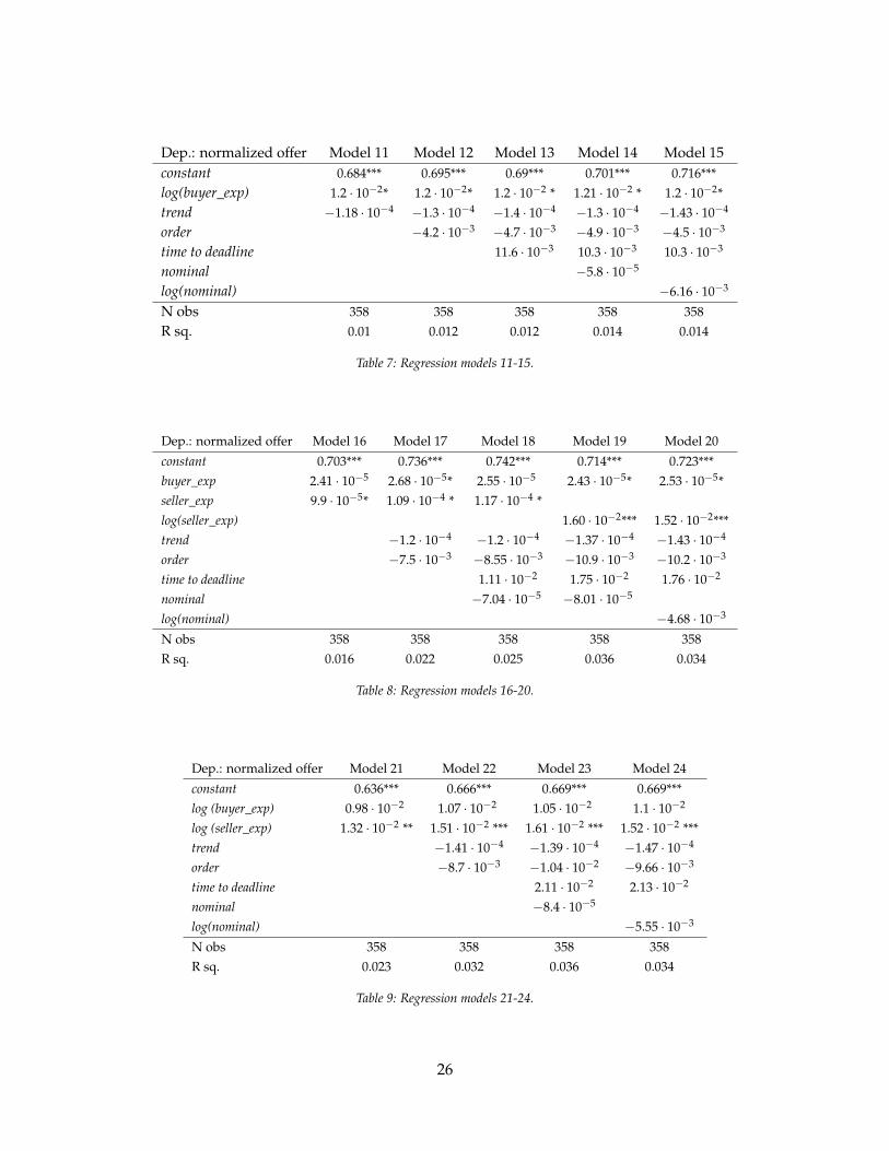
Dep.: normalized offer Model 11 Model 12 Model 13 Model 14 Model 15constant 0.684*** 0.695*** 0.69*** 0.701*** 0.716***log(buyer_exp) 1.2 · 10−2* 1.2 · 10−2* 1.2 · 10−2 * 1.21 · 10−2 * 1.2 · 10−2*trend −1.18 · 10−4 −1.3 · 10−4 −1.4 · 10−4 −1.3 · 10−4 −1.43 · 10−4
order −4.2 · 10−3 −4.7 · 10−3 −4.9 · 10−3 −4.5 · 10−3
time to deadline 11.6 · 10−3 10.3 · 10−3 10.3 · 10−3
nominal −5.8 · 10−5
log(nominal) −6.16 · 10−3
N obs 358 358 358 358 358R sq. 0.01 0.012 0.012 0.014 0.014
Table 7: Regression models 11-15.
Dep.: normalized offer Model 16 Model 17 Model 18 Model 19 Model 20
constant 0.703*** 0.736*** 0.742*** 0.714*** 0.723***buyer_exp 2.41 · 10−5 2.68 · 10−5* 2.55 · 10−5 2.43 · 10−5* 2.53 · 10−5*seller_exp 9.9 · 10−5* 1.09 · 10−4 * 1.17 · 10−4 *log(seller_exp) 1.60 · 10−2*** 1.52 · 10−2***trend −1.2 · 10−4 −1.2 · 10−4 −1.37 · 10−4 −1.43 · 10−4
order −7.5 · 10−3 −8.55 · 10−3 −10.9 · 10−3 −10.2 · 10−3
time to deadline 1.11 · 10−2 1.75 · 10−2 1.76 · 10−2
nominal −7.04 · 10−5 −8.01 · 10−5
log(nominal) −4.68 · 10−3
N obs 358 358 358 358 358R sq. 0.016 0.022 0.025 0.036 0.034
Table 8: Regression models 16-20.
Dep.: normalized offer Model 21 Model 22 Model 23 Model 24
constant 0.636*** 0.666*** 0.669*** 0.669***log (buyer_exp) 0.98 · 10−2 1.07 · 10−2 1.05 · 10−2 1.1 · 10−2
log (seller_exp) 1.32 · 10−2 ** 1.51 · 10−2 *** 1.61 · 10−2 *** 1.52 · 10−2 ***trend −1.41 · 10−4 −1.39 · 10−4 −1.47 · 10−4
order −8.7 · 10−3 −1.04 · 10−2 −9.66 · 10−3
time to deadline 2.11 · 10−2 2.13 · 10−2
nominal −8.4 · 10−5
log(nominal) −5.55 · 10−3
N obs 358 358 358 358R sq. 0.023 0.032 0.036 0.034
Table 9: Regression models 21-24.
26
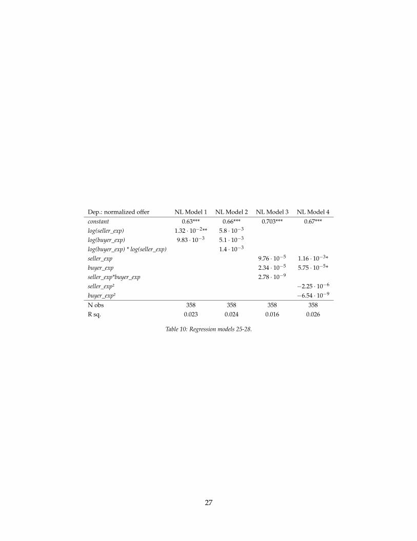
Dep.: normalized offer NL Model 1 NL Model 2 NL Model 3 NL Model 4
constant 0.63*** 0.66*** 0.703*** 0.67***log(seller_exp) 1.32 · 10−2** 5.8 · 10−3
log(buyer_exp) 9.83 · 10−3 5.1 · 10−3
log(buyer_exp) * log(seller_exp) 1.4 · 10−3
seller_exp 9.76 · 10−5 1.16 · 10−3*buyer_exp 2.34 · 10−5 5.75 · 10−5*seller_exp*buyer_exp 2.78 · 10−9
seller_exp² −2.25 · 10−6
buyer_exp² −6.54 · 10−9
N obs 358 358 358 358R sq. 0.023 0.024 0.016 0.026
Table 10: Regression models 25-28.
27

A.2.2 Decomposition
Coefficient γ0 γ1 γ2 γ3 γ4
Estimate -43.9533 73.5298 -52.4472 22.4486 -8.4939Coefficient δ0 δ1 δ2 δ3 δ4
Estimate 8.39309 -11.4105 4.53588 0.639369 -2.1579
Table 11: Chebyshev polynomial coefficients.
s: 0-10% 10-20% 20-30% 30-40% 40-50%f np (s): 25.9 7.4 3.7 18.5 44.4
c: 0-10% 10-50% 50-60% 60-70% 70-80% 80-90% 90-100%gnp (c): 14.3 7.1 5.4 17.9 23.2 21.4 10.7
Table 12: Non-parametric estimate of the distributions of sharing rules ( f ) and beliefs (g).
s: 0-10% 10-20% 20-30% 30-40% 40-50%f β (s): 23.5% 12.9% 12.0% 15.2% 36.4%
c: 0-10% 10-50% 50-60% 60-70% 70-80% 80-90% 90-100%gβ (c): 0.4% 22.1% 11.9% 14.4% 16.6% 17.9% 16.7%
Table 13: Parametric estimates when f and g are restricted to the class of β distributions. α f = 0.230, β f = 0.031;αg = 2.470, βg = 1.121, Kolmogorov-Smirnov distance = 0.066 (rejected).
28

Iter
atio
n0
12
34
56
78
910
1112
13...
50f(
b 1)
20%
14.3
%11
.1%
9.1%
14.3
%20
.0%
22.2
%26
.3%
28.6
%27
.3%
26.1
%28
.0%
26.9
%25
.9%
25.9
%f(
b 2)
20%
14.3
%11
.1%
18.2
%14
.3%
13.3
%11
.1%
10.5
%9.
5%9.
1%8.
7%8.
0%7.
7%7.
4%7.
4%f(
b 3)
20%
14.3
%11
.1%
9.1%
7.1%
6.7%
5.6%
5.3%
4.8%
4.5%
4.3%
4.0%
3.8%
3.7%
3.7%
f(b 4)
20%
28.6
%33
.3%
27.3
%28
.6%
26.7
%27
.8%
26.3
%23
.8%
22.7
%21
.7%
20.0
%19
.2%
18.5
%18
.5%
f(b 5)
20%
28.6
%33
.3%
36.4
%35
.7%
33.3
%33
.3%
31.6
%33
.3%
36.4
%39
.1%
40.0
%42
.3%
44.4
%44
.4%
g(b 1)
10%
7.1%
5.6%
4.8%
8.3%
7.7%
10.0
%9.
4%10
.5%
11.4
%12
.5%
12.5
%13
.5%
14.3
%14
.3%
g(b 2)
10%
7.1%
5.6%
4.8%
4.2%
3.8%
3.3%
3.1%
2.6%
2.3%
2.1%
2.1%
1.9%
1.8%
1.8%
g(b 3)
10%
7.1%
5.6%
4.8%
4.2%
3.8%
3.3%
3.1%
2.6%
2.3%
2.1%
2.1%
1.9%
1.8%
1.8%
g(b 4)
10%
7.1%
5.6%
4.8%
4.2%
3.8%
3.3%
3.1%
2.6%
2.3%
2.1%
2.1%
1.9%
1.8%
1.8%
g(b 5)
10%
7.1%
5.6%
4.8%
4.2%
3.8%
3.3%
3.1%
2.6%
2.3%
2.1%
2.1%
1.9%
1.8%
1.8%
g(b 6)
10%
7.1%
5.6%
4.8%
4.2%
3.8%
3.3%
3.1%
5.3%
6.8%
6.3%
6.3%
5.8%
5.4%
5.4%
g(b 7)
10%
14.3
%16
.7%
19.0
%16
.7%
15.4
%16
.7%
15.6
%15
.8%
15.9
%16
.7%
16.7
%17
.3%
17.9
%17
.9%
g(b 8)
10%
14.3
%16
.7%
19.0
%20
.8%
23.1
%23
.3%
25.0
%23
.7%
22.7
%22
.9%
22.9
%23
.1%
23.2
%23
.2%
g(b 9)
10%
14.3
%16
.7%
19.0
%20
.8%
23.1
%23
.3%
25.0
%23
.7%
22.7
%22
.9%
22.9
%23
.1%
21.4
%21
.4%
g(b 1
0)10
%14
.3%
16.7
%14
.3%
12.5
%11
.5%
10.0
%9.
4%10
.5%
11.4
%10
.4%
10.4
%9.
6%10
.7%
10.7
%
KS-
stat
0.13
640.
1658
0.06
670.
0398
0.03
270.
0264
0.01
960.
0171
0.01
430.
0127
0.01
060.
0089
0.00
810.
0077
0.00
77
Tabl
e14
:The
cons
ecut
ive
itera
tions
ofth
ebi
nary
sear
chpr
oced
ure.
29

Iter
atio
n0
12
34
56
78
910
1112
...24
...50
f (b 1)
16.7
%12
.5%
9.1%
8.3%
8.3%
13.3
%16
.7%
19.0
%21
.7%
22.2
%19
.4%
21.2
%22
.9%
23.7
%23
.7%
f (b 2)
16.7
%12
.5%
9.1%
8.3%
8.3%
6.7%
5.6%
4.8%
4.3%
3.7%
6.5%
6.1%
5.7%
8.5%
8.5%
f (b 3)
16.7
%12
.5%
9.1%
8.3%
8.3%
6.7%
5.6%
4.8%
4.3%
3.7%
3.2%
3.0%
2.9%
1.7%
1.7%
f (b 4)
16.7
%12
.5%
18.2
%16
.7%
16.7
%20
.0%
22.2
%19
.0%
17.4
%18
.5%
19.4
%21
.2%
22.9
%16
.9%
16.9
%f (
b 5)
16.7
%25
.0%
27.3
%33
.3%
33.3
%33
.3%
33.3
%33
.3%
34.8
%33
.3%
32.3
%30
.3%
28.6
%37
.3%
37.3
%f (
b 6)
16.7
%25
.0%
27.3
%25
.0%
25.0
%20
.0%
16.7
%19
.0%
17.4
%18
.5%
19.4
%18
.2%
17.1
%11
.9%
11.9
%
g(b
1)10
.0%
7.1%
5.6%
4.5%
7.7%
7.4%
9.4%
11.1
%10
.8%
12.2
%13
.3%
13.0
%13
.7%
15.6
%15
.6%
g(b
2)10
.0%
7.1%
5.6%
9.1%
7.7%
7.4%
6.3%
5.6%
5.4%
4.9%
4.4%
4.3%
3.9%
2.6%
2.6%
g(b
3)10
.0%
7.1%
5.6%
4.5%
3.8%
3.7%
3.1%
2.8%
2.7%
2.4%
2.2%
2.2%
2.0%
1.3%
1.3%
g(b
4)10
.0%
7.1%
5.6%
4.5%
3.8%
3.7%
3.1%
2.8%
2.7%
2.4%
2.2%
2.2%
2.0%
1.3%
1.3%
g(b
5)10
.0%
7.1%
5.6%
4.5%
3.8%
3.7%
3.1%
2.8%
2.7%
2.4%
2.2%
2.2%
2.0%
2.6%
2.6%
g(b
6)10
.0%
7.1%
11.1
%9.
1%7.
7%7.
4%6.
3%5.
6%5.
4%4.
9%4.
4%4.
3%3.
9%2.
6%2.
6%g(b
7)10
.0%
14.3
%16
.7%
18.2
%19
.2%
18.5
%18
.8%
19.4
%18
.9%
19.5
%20
.0%
19.6
%19
.6%
19.5
%19
.5%
g(b
8)10
.0%
14.3
%16
.7%
18.2
%19
.2%
18.5
%18
.8%
19.4
%21
.6%
22.0
%22
.2%
23.9
%23
.5%
27.3
%27
.3%
g(b
9)10
.0%
14.3
%16
.7%
18.2
%19
.2%
22.2
%21
.9%
22.2
%21
.6%
22.0
%22
.2%
21.7
%21
.6%
19.5
%19
.5%
g(b
10)
10.0
%14
.3%
11.1
%9.
1%7.
7%7.
4%9.
4%8.
3%8.
1%7.
3%6.
7%6.
5%7.
8%7.
8%7.
8%
KS
0.12
500.
0550
0.04
110.
0361
0.03
220.
0271
0.02
310.
0190
0.01
710.
0161
0.01
510.
0129
0.00
660.
0066
Tabl
e15
:The
cons
ecut
ive
itera
tions
ofth
ebi
nary
sear
chpr
oced
ure,
with
rest
rict
ion
0.6.
30

A.3 Figures
Figure 6: Smooth kernel histograms for the offers made by the East (red) and the West German participants (blue).
Figure 7: The histogram of the normalized offers (grey bars) and smooth kernel histograms for the offers made first (blue)and all the higher-order offers (red).
31

A.4 Robustness Checks
A.4.1 Note: Non-parametric Decomposition
As an alternative way to solve for f and g, we discretize the support of distributions in(3) and we search for finite solution approximations using a non-parametric approach. Inan iterative procedure with the initial state where both f and g are uniform, we graduallyincrease precision until the solution cannot be improved. The estimates of f and g are chosento minimize the Kolmogorov-Smirnov distance as a goodness-of-fit criterion, adapted to thediscrete case:
dKS(
H, H)≡ sup{bk}k=1,..,10
∣∣H (bk)− H (bk)∣∣ , (12)
where both H and H are defined on a set of bins (b1,b2, ..,b10) = (0.1,0.2, ..,1). In thediscrete problem, we look for f and g that minimize (12), subject to f (bk) = 0 for k = 6,7, ..,10,and ∑k f (bk) = ∑k g (bk) = 1. (Recall that f and g define H according to (8)).
We estimate discretized versions of f and g simultaneously at each iteration. As a startingpoint of recurrence, we consider uniform f and g that correspond to the maximal entropy inboth c and s (See Table 14 in the Appendix). That is, we assign equal mass to each of the 5bins of f and 10 bins of g at the first iteration. The candidate solution can be represented asa vector of ones: v1 = (1,1, ..,1); it corresponds to the distribution of probability mass acrossbins before normalization. v1 is the unique candidate solution at the first iteration, thus weset v∗1 = v1 At the second iteration, we consider all elements e2,k of the set {0,1}15 and therespective v2,k = v1 + e2,k. This gives 215 = 32768 candidate solutions ( f , g) and we choose theone that minimizes the Kolmogorov-Smirnov distance (after the appropriate normalization)– v∗2 . Generally, in iteration t, we go through all possible constellations of adding one unit ornot changing the mass in the bins of distributions defined by v∗t−1 selected at iteration t− 1.Among the pairs of f and gn we select the one that minimizes the Kolmogorov-Smirnovdistance and take it to iteration t + 1. The process is repeated until the result at a subse-quent iteration stays unchanged. Note that as the depth of the binary search tree increases,the estimates become increasingly precise. The results of the non-parametric approach arepresented in Table 12.
Define Hnp as in (8) by substituting in f = f np and g = gnp from Table 12. H∗ is anextremely good fit for H: the Kolmogorov-Smirnov distance is 7.7× 10⁻³, meaning that themaximal divergence between Hnp and H across bins is less than 1 percentage point. Thecorresponding bootstrap test does not distinguish between H and Hnp at the conventional
32

significance levels,34 implying that H and H∗bp can be regarded as equivalent.
As a further robustness check, we relax the restriction on the support of f allowing sixbins; similar results are obtained (see Table 15).
A.4.2 Note: Parametric Decomposition with Beta Distributions.
As a further robustness check, we look for estimates f β and gβ within the class of the betadistributions. The beta class is chosen due to its support on [0, 1], small number of param-eters and flexibility, as Beta distributions can have one or two modes.35 Since each of thedistributions f and g is pinned down by two parameters, the problem to find the suitableH(.) in (7) is now (only) four-dimensional. We estimate the parameters by random gridsearch. More precisely, we fix a grid size for each of four parameters and randomly choosethe grid position. For every intersection of the grid (a combination of four parameter values),we compute the discretized versions of f and g, estimate the integral (8), then we calculatethe Kolmogorov-Smirnov distance and reiterate to find the best-performing combination ofparameters. By performing the procedure multiple times, we refine the search and narrowdown the parameters ranges. A random grid search permits us to trace out local minimaand find the global solution. We report the parametric estimates of distributions f β and gβ
Table 13. The parametric Beta estimates f β and gβ are dominated by both the parametric andthe non-parametric solutions reported in the main text of the paper (Kolmogorov-Smirnovdistance = 0.066). The distributions have a shape similar to the non-parametric estimates f ∗
and g∗, with the exception of the lowest bin in the distribution of cost estimates g.
34Bootstrap critical values corresponding to 358 observations are 0.049 for significance at 10%, 0.057 for sig-nificance at 5%, and 0.071 for significance at 1%.
35Excluding the uniform distribution.
33

References
ALESINA, A. AND N. FUCHS-SCHUENDELN (2005): “Good bye Lenin (or not?): The effect ofCommunism on people’s preferences,” Tech. rep., National Bureau of Economic Research.
ALGER, I. AND J. W. WEIBULL (2013): “Homo moralis – preference evolution under incom-plete information and assortative matching,” Econometrica, 81, 2269–2302.
BEARDEN, J. (2001): “Ultimatum Bargaining Experiments: The State of the Art,” Workingpaper, INSEAD – Decision Sciences.
BINMORE, K., J. SWIERZBINSKI, AND C. TOMLINSON (2007): “An experimental test of Ru-binstein’s bargaining model,” Working paper, ESRC Centre for Economic Learning andSocial Evolution.
BOEHM, C., H. B. BARCLAY, R. K. DENTAN, M.-C. DUPRE, J. D. HILL, S. KENT, B. M.KNAUFT, K. F. OTTERBEIN, AND S. RAYNER (1993): “Egalitarian behavior and reversedominance hierarchy [and comments and reply],” Current Anthropology, 34, 227–254.
BOLTON, G. E. AND A. OCKENFELS (2014): “Does laboratory trading mirror behavior in realworld markets? Fair bargaining and competitive bidding on eBay,” Journal of EconomicBehavior & Organization, 97, 143–154.
BROSIG-KOCH, J., C. HELBACH, A. OCKENFELS, AND J. WEIMANN (2011): “Still differentafter all these years: Solidarity behavior in East and West Germany,” Journal of Public Eco-nomics, 95, 1373–1376.
CABRAL, L. AND A. HORTASCU (2010): “The dynamics of seller reputation: Evidence fromeBay,” The Journal of Industrial Economics, 58, 54–78.
CAMERER, C. (2003): Behavioral game theory: Experiments in strategic interaction, Princeton, NJ:Cambridge University Press.
CAMERON, L. A. (1999): “Raising the stakes in the ultimatum game: Experimental evidencefrom Indonesia,” Economic Inquiry, 37, 47–59.
CARD, D., S. DELLAVIGNA, AND U. MALMENDIER (2011): “The Role of Theory in FieldExperiments,” Journal of Economic Perspectives, 25, 39–62.
CHARNESS, G. AND M. RABIN (2002): “Understanding Social Preferences with SimpleTests,” The Quarterly Journal of Economics, 117, 817–869.
DUFWENBERG, M. AND G. KIRCHSTEIGER (2004): “A theory of sequential reciprocity,”Games and Economic Behavior, 47, 268 – 298.
34

ELY, J. C. AND T. HOSSAIN (2009): “Sniping and Squatting in Auction Markets,” AmericanEconomic Journal: Microeconomics, 1, 68–94.
FALK, A. AND U. FISCHBACHER (2006): “A theory of reciprocity,” Games and Economic Be-havior, 54, 293 – 315.
FEHR, E. AND K. M. SCHMIDT (1999): “A Theory of Fairness, Competition, and Coopera-tion,” The Quarterly Journal of Economics, 114, 817–868.
FEHR-DUDA, H., A. BRUHIN, T. EPPER, AND R. SCHUBERT (2010): “Rationality on the rise:Why relative risk aversion increases with stake size,” Journal of Risk and Uncertainty, 40,147–180.
FISCHBACHER, U., C. FONG, AND E. FEHR (2009): “Fairness, Error and the Power of Com-petition,” Journal of Economic Behaviour and Organization, 72, 527–545.
FUKUYAMA, F. (1995): Trust: The social virtues and the creation of prosperity, Free Press NewYork.
GALIZZI, M. M. AND D. NAVARRO MARTINEZ (2015): “On the external validity of social-preference games: A systematic lab-field study,” Working paper, Barcelona GraduateSchool of Economics.
GIBBS, J., K. L. KRAEMER, AND J. DEDRICK (2003): “Environment and policy factors shapingglobal e-commerce diffusion: A cross-country comparison,” The information society, 19, 5–18.
GIGERENZER, G. (2007): Gut feelings: The intelligence of the unconscious, Penguin.
GÜTH, W. AND M. KOCHER (2013): “More than Thirty Years of Ultimatum Bargaining Ex-periments: Motives, Variations, and a Survey of the Recent Literature,” Working paper,Max Planck Instute of Economics and CESifo.
GÜTH, W., R. SCHMITTBERGER, AND B. SCHWARZE (1982): “An experimental analysis ofultimatum bargaining,” Journal of Economic Behaviour and Organization, 3, 367–388.
HARRISON, G. W. AND J. A. LIST (2004): “Field experiments,” Journal of Economic literature,42, 1009–1055.
HENRICH, J., R. MCELREATH, A. BARR, J. ENSMINGER, C. BARRETT, A. BOLYANATZ, J. C.CARDENAS, M. GURVEN, E. GWAKO, N. HENRICH, ET AL. (2006): “Costly punishmentacross human societies,” Science, 312, 1767–1770.
HOFFMAN, E., K. MCCABE, AND V. SMITH (1996): “On expectations and the monetarystakes in ultimatum games,” International Journal of Game Theory, 25, 289–301.
35

HOLT, C. AND S. LAURY (2002): “Risk Aversion and Incentive Effects,” American EconomicReview, 92, 1644–1655.
JOHN, K. AND S. L. THOMSEN (2013): “Environment and other-regarding preferences,”Tech. rep., Discussion Paper 4, Niedersächsisches Institut für Wirtschaftsforschung, Han-nover.
LEVITT, S. D. AND J. A. LIST (2007): “What do laboratory experiments measuring socialpreferences reveal about the real world?” The journal of economic perspectives, 21, 153–174.
——— (2009): “Field experiments in economics: The past, the present, and the future,” Eu-ropean Economic Review, 53, 1 – 18.
LIST, J. A. (2006): “The Behavioralist Meets the Market: Measuring Social Preferences andReputation Effects in Actual Transactions,” Journal of Political Economy, 114.
——— (2011): “Why Economists Should Conduct Field Experiments and 14 Tips for PullingOne Off,” Journal of Economic Perspectives, 25, 3–16.
MALMENDIER, U. AND Y. H. LEE (2011): “The bidder’s curse,” The American Economic Re-view, 749–787.
MATHEMATICA (2015): Version 10, Wolfram Research, Inc., Champaign, IL.
MUNIER, B. AND C. ZAHARIA (2002): “High stakes and acceptance behavior in ultimatumbargaining,” Theory and Decision, 53, 187–207.
NEWELL, A., H. A. SIMON, ET AL. (1972): Human problem solving, vol. 104, Prentice-Hall.
NOSKO, C. AND S. TADELIS (2015): “The limits of reputation in platform markets: An em-pirical analysis and field experiment,” Working paper, National Bureau of Economic Re-search.
OCKENFELS, A. AND G. E. BOLTON (2000): “ERC: A Theory of Equity, Reciprocity, andCompetition,” American Economic Review, 90, 166–193.
OCKENFELS, A. AND J. WEIMANN (1999): “Types and patterns: an experimental East-West-German comparison of cooperation and solidarity,” Journal of Public Economics, 71, 275–287.
OOSTERBEEK, H., R. SLOOF, AND G. VAN DE KUILEN (2004): “Cultural Differences in Ul-timatum Game Experiments: Evidence from a Meta-Analysis,” Experimental Economics, 7,171–188.
36

RABIN, M. (1993): “Incorporating Fairness into Game Theory and Economics,” AmericanEconomic Review, 83, 1281–1302.
RESNICK, P., R. ZECKHAUSER, J. SWANSON, AND K. LOCKWOOD (2006): “The value ofreputation on eBay: A controlled experiment,” Experimental Economics, 9, 79–101.
ROTH, A., V. PRASNIKAR, M. OKUNO-FUJIWARA, AND S. ZAMIR (1991): “Bargaining andMarket Behaviour in Jerusalem, Ljubljana, Pittsburgh and Tokyo,” American Economic Re-view, 81, 1068–1095.
ROTH, A. E. AND I. EREV (1995): “Learning in extensive-form games: Experimental dataand simple dynamic models in the intermediate term,” Games and Economic Behavior, 8,164 – 212.
ROTH, A. E. AND A. OCKENFELS (2002): “Last-Minute Bidding and the Rules for EndingSecond-Price Auctions: Evidence from eBay and Amazon Auctions on the Internet,” Amer-ican Economic Review, 92, 1093–1103.
RUBINSTEIN, A. (1982): “Perfect equilibrium in a bargaining model,” Econometrica: Journal ofthe Econometric Society, 97–109.
SADOVNICHY, V. (1986): Theory of Operators (in Russian), Moscow State University.
SELTEN, R. (1965): “Spieltheoretische behandlung eines oligopolmodells mit nach-frageträgheit: Teil i: Bestimmung des dynamischen preisgleichgewichts,” Zeitschrift fürdie gesamte Staatswissenschaft/Journal of Institutional and Theoretical Economics, 301–324.
SLONIM, R. AND A. E. ROTH (1998): “Learning in high stakes ultimatum games: An experi-ment in the Slovak Republic,” Econometrica, 569–596.
THOMSON, W. (1994): “Cooperative models of bargaining,” Handbook of game theory witheconomic applications, 2, 1237–1284.
TVERSKY, A. AND D. KAHNEMAN (1974): “Judgment under uncertainty: Heuristics andbiases,” science, 185, 1124–1131.
VAN DAMME, E., K. G. BINMORE, A. E. ROTH, L. SAMUELSON, E. WINTER, G. E. BOLTON,A. OCKENFELS, M. DUFWENBERG, G. KIRCHSTEIGER, U. GNEEZY, M. G. KOCHER,M. SUTTER, A. G. SANFEY, H. KLIEMT, R. SELTEN, R. NAGEL, AND O. H. AZAR (2014):“How Werner Güth’s ultimatum game shaped our understanding of social behavior,” Jour-nal of Economic Behavior and Organization, 108, 292–318.
37