selling info sept 4 - stanford universityskrz/selling_info.pdf · jel codes: c72, d82, d83 ... case...
TRANSCRIPT
Selling Information∗
Johannes Horner† and Andrzej Skrzypacz‡
September 5, 2014
Abstract
A Firm considers hiring an Agent who may be competent for a potential project or not.
The Agent can prove her competence, but faces a hold-up problem. We propose a model of
persuasion and show how gradualism helps mitigate the hold-up problem. We show when
it is optimal to give away part of the information at the beginning of the bargaining, and
sell the remainder in dribs and drabs. The Agent can only appropriate part of the value of
information. Introducing a third-party allows her to extract the maximum surplus.
Keywords: value of information, dynamic game.
JEL codes: C72, D82, D83
∗We thank Daron Acemoglu, Robert Aumann, Hector Chade, Alex Frankel, Drew Fudenberg, David Kreps,Max Kwiek, R. Vijay Krishna, Sofia Moroni, Romans Pancs, Arthur Robson, Rann Smorodinsky and seminarparticipants at the Barcelona JOCS, the Collegio Carlo Alberto, Turin, Essex University, the European UniversityInstitute, Harvard-MIT, University of Illinois at Urbana-Champaign, Northwestern University, Oxford University,Simon Fraser University, Stanford University, University of British Columbia, University of Western Ontario, UCSan Diego, Yale, X-HEC Paris, Paris Sciences Economiques, Toulouse School of Economics, the European SummerSymposium in Economic Theory at Gerzensee 2012, the SED 2009 meeting, the Stony Brook 2010 game theoryconference, and the 2011 Asian meeting of the Econometric Society for useful comments and suggestions.
†Yale University, 30 Hillhouse Ave., New Haven, CT 06520, USA. [email protected].‡Stanford University, Graduate School of Business, 518 Memorial Way, Stanford, CA 94305, USA.
1
1 Introduction
A firm contemplates hiring an expert for a potential project. For example, the firm considers
hiring a consulting company to lead a potential re-organization of its division; the firm considers
hiring an advisor to help with a potential acquisition, or an inventor to help build a new product
feature, or a product itself, in the case of an agency engaged in a procurement process.
The agent has private information whether she is competent (type 1) or incompetent (type
0). Hiring an incompetent agent leads to a negative expected net present value (ENPV) from
the project. Hiring a competent agent yields a positive ENPV. While the firm could hire the
expert/agent by offering her a payment equal to her outside option, the firm’s problem is that
it is uncertain whether hiring the agent and going forward with the project is the best course of
action. The firm could take its decision based on the prior belief, but taking into account the
agent’s information would result in efficiency gains.
How could the agent persuade the firm that she is competent and at the same time be
rewarded for competence? How should the agent sell that information optimally so that the firm
would make an informed hiring decision and the agent would be utmost motivated to acquire
competence?
To answer these questions, we propose a game-theoretic model of gradual persuasion between
the Agent and the Firm. Persuasion can be thought of as preliminary projects, or temporary
employment spells (that either side can revoke at any time). During the trial period the Agent
is paid and gradually reveals information. In particular, the Agent performs tasks (that we call
“tests”) that are informative about her type. In every period, the Firm observes the task chosen
by the Agent, its outcomes and then decides whether to continue the trial period, fire the Agent,
or hire her and start the main project. Neither the Firm nor the Agent can commit to future
payments, hiring decisions, test-taking (choice of tasks) or information sharing. There is neither
commitment nor contractibility. Most importantly, the Firm cannot commit to pay the Agent
contingent on the information she reveals. In practice, there are obvious ways in which the two
sides can commit, more or less formally. The Agent might be concerned about her reputation
for competence, for instance. The legal structure might provide some protection to intellectual
property rights (as patents do).
2
Motivated by incentives to acquire competence, we characterize equilibria that maximize the
difference in expected payoffs of the Agent of type 1 and type 0 (as we show, this is equivalent
to solving for equilibria that maximize the payoffs of the competent agent).
With one-time information transmission (whether information disclosure is full or partial)
both types of the Agent would get the same payment. Maximizing incentives to acquire compe-
tence calls for multi-stage communication. The game we consider is therefore dynamic: there is
a multi-stage information selling stage (which we call the game of information sale) followed by
the final decision of the Firm, that depends on the information the Firm has acquired. Within a
round of communication, the two parties make voluntary monetary transfers and then the Agent
can disclose some information to the Firm.
We assume that information is verifiable and divisible. In particular, the information trans-
mission is modeled as tests to verify the Agent’s type. Verifiability of information means that each
test has a known difficulty: the competent Agent can always pass it (in the baseline model), but
the incompetent Agent passes it with a probability commensurate to its difficulty. Easier tests
have a higher probability of being passed by an incompetent Agent. Divisibility of information
means that there is a rich set of available tests of varying difficulties.
Our main result is that, very generally, “splitting information over time” increases the com-
petent Agent’s payoff. That is, the competent Agent’s payoff is higher in equilibria in which
she takes two tests (and is paid for them) in a sequence, than if she takes both of them at once
(which is equivalent to taking one harder test). The intuition is that when we split the tests, the
Firm pays still the same amount on average, but the incompetent Agent may fail the first test,
so that type gets a smaller fraction of the expected payment.
That effect explains the structure of the best equilibrium in our first model: first, an initial
chunk of information is given away for free that leads the Firm to utmost confusion regarding
whether hiring the agent is the correct decision. If the Agent passes this first test, she is then
hired on a “temporary basis,” and during the trial, as long as the Agent performs, she sells
information in dribs and drabs and gets paid a little for each bit (and a failure of a test leads
to a termination). These features seem consistent with the practice of preliminary reports/trial
periods before firms make large financial commitments to projects with the help of external
3
experts. Our finding that selling information gradually is beneficial to reward competence of the
seller should come as no surprise to anyone who was ever involved in consulting. The free first
consultation is also reminiscent of standard business practice.
We derive a tight bound on the competent Agent’s equilibrium payoff as the number of
possible communication rounds grows to infinity. Although the closed-form expression for the
limit payoff relies on the divisibility of information and the arbitrary number of rounds that we
allow, there is no discontinuity: the benefit of splitting information does not depend on either
assumption.
While the acquisition of competence is our leading interpretation for the model, we also
develop a more general version that could be useful for other applications. For example, the
Firm may be buying the Agent’s advice (not needing the Agent’s help to execute the project)
and the Agent could be privately informed about a state of the world, which in turn affects the
ENPV of the project. The Firm’s action set does not need to be binary either (for example,
the Firm may be choosing a size of its investment in the project). To model such situations, we
allow for more general payoffs if the Firm decides to make decisions without further information
from the Agent. In particular, these payoffs capture the possibility that revealing information
the Agent has about the state makes it easier for the Firm to make good decisions without
further Agent’s input. We show that the benefits of “splitting information” apply to this more
general model and characterize the best equilibrium payoffs for the type-1. We prove that selling
information in small bits is profitable as long as the Firm’s payoff function (mapping the current
posterior belief to Firm’s ENPV if it was to make a decision without any further information
from the Agent) is star-shaped, that is, as long as its average value is increasing in the belief.
Splitting information might help the Agent in extracting more surplus from the relationship,
but it does not suffice to extract the entire surplus. In the last section of the paper we show
how enlarging the class of “test technologies” to include some that involve noisy communication
between the Agent and the Firm can help. In particular, we show that, even with our extreme
assumptions of non-contractibility and non-commitment, with rich enough tests, the competent
Agent can extract the entire expected value quite generally.
4
Related Literature: The paper is related to the literature on hold-up, for example Gul (2001)
and Che and Sakovics (2004). One difference is that in our game what is being sold is information
and hence the value of past pieces sold can depend on the future pieces that are disclosed (or
failed to be). An agent that eventually reveals himself to be incompetent destroys by the same
token the value of the consideration that he had established. This property of beliefs –that
they can go up or down– is an essential ingredient for our results. Moreover, we assume that
there is no physical cost of selling a piece of information and hence the Agent does not care per
se about how much information the Firm gets or what action it takes. In contrast, in Che and
Sakovics (2004) each piece of the project is costly to the Agent and the problem is how to provide
incentives for this observable effort.
The formal maximization problem, and in particular the structural constraints on information
revelation, are reminiscent of the literature on long cheap talk. See, in particular, Forges (1990)
and Aumann and Hart (2003), and, more generally, Aumann and Maschler (1995). As is the
case here, the problem is how to “split” a martingale optimally over time. That is, the Firm’s
belief is a martingale, and the optimal strategy specifies its distribution over time. Ely, Frankel
and Kamenica (2013) is another analysis of optimal martingale splitting, although information
has instrumental value there.
There are important differences between our paper and the motivation of these papers, how-
ever. First and foremost, unlike in that literature, payoff-relevant actions are taken before infor-
mation disclosure is over, since the Firm pays the Agent as information gets revealed over time,
so communication and payments are concurrent here. In fact, with a mediator, the Agent also
makes payments to the Firm during the communication phase. As in Matthews and Postlewaite
(1995) or Forges and Koessler (2008), messages are type-dependent, as the Agent is constrained
in the messages she can send by the information she actually owns. Pure cheap-talk (i.e., the
possibility to send messages from sets that are type-independent) is of no help in our model.
Rosenberg, Solan and Vieille (2013) consider the problem of information exchange between two
informed parties in a repeated game without transfers, and establish a folk theorem. In all these
papers, the focus is on identifying the best equilibrium from the Agent’s perspective in the ex
ante sense, before her type is known. In our case, this is trivial and does not deliver differential
5
payoffs to the Agent’s types (i.e., a higher payoff to the competent type).
The martingale property is distinctive of information, and this is a key difference between our
set-up and other models in which gradualism appears. In particular, the benefits of gradualism
are well known in games of public goods provision (see Admati and Perry, 1991, Compte and
Jehiel, 2004 and Marx and Matthews, 2000). Contributions are costly in these games, whereas
information disclosure is not costly per se. In fact, costlessness is a second hallmark of information
disclosure that plays an important role in the analysis. (On the other hand, the specific order of
moves is irrelevant for the results, unlike in contribution games.) The opportunity cost of giving
information away is a function of the equilibrium to be played. So, unlike in public goods game,
the marginal (opportunity) cost of information is endogenous. Relative to sales of private goods,
the marginal value of information cannot be ascertained without considering the information as
a whole, very much as for public goods.
Our focus (proving one’s knowledge) and instrument (tests that imperfectly discriminate for
it) are reminiscent of the literature on zero-knowledge proofs, which also stresses the benefits
of repeating such tests. This literature that starts with the paper of Goldwasser, Micali and
Rackoff (1985) is too large to survey here. A key difference is that, in that literature, passing
a test conveys information about the type without revealing anything valuable (factoring large
numbers into primes does not help the tester factoring numbers himself). In many economic
applications, however, it is hard to convince the buyer that the seller has information without
giving away some of it, which is costly –as it is in our model.
Indeed, unlike in public goods games, or zero-knowledge proofs, splitting information is not
always optimal. As mentioned, this hinges on a (commonly satisfied) property of the Firm’s
payoff, as a function of its belief about the Agent’s type.
Our leading motivating example of an agent that tries to convince a firm to hire her is
closely related to that of the standard model of signaling, as in Spence (1973). There are three
differences. First, in terms of technology: In job market signaling, all messages can be sent
by all types, but at different costs. Here instead, messages are free, but the message space is
type-dependent. Second, in terms of market structure: in standard job market signaling, it is
usually assumed that firms compete for the worker, who reaps the entire surplus, so the issue
6
of how much surplus signaling allows her to appropriate does not really come up. Third, in
terms of objective function: our goal is to understand what equilibrium maximizes the payoff
difference between the competent and incompetent type, a question that isn’t usually central to
the analysis of signaling. These are not major differences, however: type-dependent messages
can be viewed as actions that are prohibitively costly to some types;1 perfect competition among
firms does not seem like an essential ingredient of Spence’s analysis, and likewise for the fact that
we ignore here any outside option for the agent. The major difference, in our view, is that we are
interested in how persuasion should be dynamically structured, to provide maximum rewards for
(and so incentives to acquire) competence. With the exception of Forges (1990), who analyzes a
very different game, we are not aware of an analysis of longer communication or signaling in a
job market related setting.
Less related are some papers in industrial organization. Our paper is complementary to Anton
and Yao (1994 and 2002) in which an inventor tries to obtain a return to his information in the
absence of property rights. In Anton and Yao (1994) the inventor has the threat of revealing
information to competitors of the Firm and it allows him to receive payments even after she
gives the Firm all information. In Anton and Yao (2002) some contingent payments are allowed
and the inventor can use them together with competition among firms to obtain positive return
to her information. In contrast, in our model, there are no contingent payments and we assume
that only one Firm can use the information.
Finally, there is a vast literature directly related to the value of information. See, among
others, Admati and Pfleiderer (1988 and 1990). Eso and Szentes (2007) take a mechanism design
approach to this problem, while Kamenica and Gentzkow (2011) apply ideas similar to Aumann
and Maschler (1995) to study optimal information disclosure policy when the Agent does not
have private information about the state of the world, but cares about the Firm’s action.
1Although this interpretation of our tests does not quite work, because the incompetent agent does not knowwhether she will be lucky or not in passing a given test.
7
2 Hiring Competent Experts and Motivating Competence
We start with a simple model in which we explicitly derive how the Firm’s payoff of hiring the
Agent as a function of the Firm’s beliefs about her competence arises from a decision problem.
2.1 Set-Up
There is one Agent (she) and a Firm (it). The Agent is of one of two possible types: ω ∈Ω := 0, 1 , she is either competent (1) or not (0). We also refer to these as type-1 and type-0.
The Agent’s type is private information. The Firm’s prior belief that ω = 1 is p0 ∈ (0, 1). In
Section 2.6, we discuss how this belief might come about.
The game is divided into K rounds of communication (we focus on the limit as K grows
large), followed by an action stage. In the action stage the Firm must choose either action I
(hire the agent and “Invest”in the project) or N (not hire the agent and “Not Invest”in the
project). Not Investing yields a payoff of 0 independently of the Agent’s type. Investing yields
an expected net payoff of 1 if ω = 1 and −γ < 0 if ω = 0 (net of the costs of hiring the Agent).
That is, investing is optimal if the Agent is competent, as such an Agent has the skill, know-how,
or information to make the investment thrive. However, if the Agent is incompetent, it is safer
to abstain from investing.
In each of the K rounds of communication timing is as follows. First, the Firm and the Agent
choose a monetary transfer to the other player, tAk and tFk , respectively.2 Second, after these
simultaneous transfers, the Agent chooses whether to reveal some information by undergoing a
test.3
We propose the following concrete model of gradual persuasion/communication using tests.
We assume that for every m ∈ [0, 1], there exists a test that the competent Agent passes for
sure, but that the incompetent Agent passes with probability m. The level of difficulty, m, is
2The Reader might wonder why we allow the Agent to pay the Firm. After all, it is the Agent who owns theunique valuable good, information. Such payments will turn out to be irrelevant given the testing technology inthis section, but will play a role in the second part of the paper with more complex communication.
3Nothing hinges on this timing. Payments could be made sequentially rather than simultaneously, and occurafter rather than before the test is taken.
8
chosen by the Agent and observed by the Firm.4 If the Firm’s prior belief about the Agent being
competent is p and a test of difficulty m is chosen and passed, the posterior belief is
p′ =p
p+ (1− p)m.
Thus, the range of possible posterior beliefs as m varies is [p, 1] (if the test is passed). An
uninformative test corresponds to the case m = 1. If the Agent fails the test, then the Firm
correctly updates its belief to zero. To allow for rich communication, tests of any desired precision
m are available at each of the K rounds, and their outcomes are conditionally independent.
In words, by disclosing information, the Agent affects the Firm’s belief that she is competent.
Persuasion can be a gradual process: after the Agent discloses some information, the Firm’s
posterior belief p′ can be arbitrary, provided the prior belief p is not degenerate. But the Firm uses
Bayesian updating. Viewed as a stochastic process whose realization depends on the disclosed
information, the sequence of posterior beliefs is a martingale from the Firm’s point of view. 5
2.2 Histories, Strategies and Payoffs
More formally, a (public) history of length k is a sequence
hk = (tAk′, tFk′, mk′, rk′)k−1k′=0,
where (tAk′, tFk′, mk′, rk′) ∈ R
2+ × [0, 1]× 0, 1. Here, mk is the difficulty of the test chosen by the
Agent in stage k and rk is the outcome of that test (which is either positive, 1, or negative, 0).
4Because the level of difficulty is determined in equilibrium, it does not matter that the Agent chooses it ratherthan the Firm.
5More abstractly, as in the literature on repeated games with incomplete information, we can think of anAgent’s strategy as a choice of a martingale –the Firm’s beliefs– given the consistency requirements imposed byBayes’ rule. For concreteness, we model this as the outcome of a series of tests whose difficulty can be varied.Alternatively, we may think of information as being divisible, and the Agent choosing how much information todisclose at each round; the incompetent Agent might be a charlatan who might be lucky or skilled enough toproduce some persuasive evidence. For now, we do not allow the competent Agent to flunk the test on purpose,nor do we consider tests so difficult that even the competent Agent might fail them. This means that the samplepath of the belief martingale is either non-decreasing, or absorbed at zero. We discuss richer communicationpossibilities in Section 4.
9
The set of all such histories is denoted Hk (set H0 := ∅).
A (behavior) strategy σF for the Firm is a collection (τFk K−1k=0 , α
F ), where (i) τFk is a prob-
ability transition τFk : Hk → R+, specifying a transfer tFk := τF (hk) as a function of the (public)
history so far, as well as (ii) an action (a probability transition as well), αF : HK → I, N after
the K-th round. A (behavior) strategy σA for the Agent is a collection τAk , µAk K−1
k=0 , where (i)
τAk : Ω × Hk → R+ is a probability transition specifying the transfer tAk := τA(hk) in round k
given the history so far and given the information she has, (ii) µAk : Ω × Hk × R
2+ → [0, 1] is a
probability transition specifying the difficulty of the test (i.e., the value of m), as a function of
the Agent’s type, the history up to the current round, and the transfers that were made in the
round. All choices are possibly randomized, but in this and next section we restrict attention to
pure-strategy equilibria.
These definitions imply that there is no commitment on either side: the Firm (and the Agent)
can stop making payments at any time, and nothing compels the Agent to disclose information
if she prefers not to.
In terms of payoffs, we assume there is neither discounting nor any other type of frictions
during the K rounds (for example, taking the tests is free). We discuss frictions in the next
section.
Absent any additional information revelation, the Firm’s optimal action is to invest if and
only if its belief p that her type is 1 satisfies
p ≥ p∗ :=γ
1 + γ.
Hence, its payoff from the optimal action is given by
w(p) := [p− (1− p)γ]+,
where x+ := max0, x. While our analysis covers both the case in which the prior belief p0 is
below or above p∗, we have in mind the more interesting case in which p0 is smaller than p∗.
The payoff w(p) is the Firm’s outside option. Since we assumed that the firm makes a binary
investment decision, the specific outside option reduces to a call option. We consider a richer
10
class of outside option specifications in the next section.
To focus attention on the communication stage of the game, we assume for now that if the
Firm decides to invest, it hires the Agent at a salary equal to her outside option (we consider
the perhaps more realistic case in which the Agent strictly prefers to be hired in section 2.5).
As a result, the Agent does not care about the Firm’s investment decision or about its own
competence per se. All she cares about is getting paid as much as possible over the K rounds of
communication.
The Firm cares about the payoff from the investment decision, net of any payments to the
Agent during the communication stage (recall that the investment payoffs already include the
cost of hiring the Agent).
Given some final history hK (which does not include the Firm’s final action to invest or not),
type-ω Agent’s realized payoff is the sum of all net transfers over all rounds, independently of
her type:
Vω(hK) =
K−1∑
k=0
(τFk − τAk ).
Given type ω, the Firm’s overall payoff results from its action, as well as from the sum of net
transfers. If the Firm chooses the safe action, it gets
W (ω, hK , N) =
K−1∑
k=0
(τAk − τF
k ).
If instead the Firm decides to invest, it receives
W (ω, hK , I) =K−1∑
k=0
(τAk − τFk ) + 1 · 1ω=1 − γ · 1ω=0,
where 1A denotes the indicator function of the event A.
A prior belief p0 and a strategy profile σ := (σF , σA) define a distribution over Ω×HK×I, N,and we let V (σ),W (σ), or simply V,W , denote the expected payoffs of the Agent and the Firm,
respectively, with respect to this distribution. When the strategy profile is understood, we also
write V (hk),W (hk) for the players’ continuation payoffs, given history hk. We further write
11
V0, V1, for the payoff to the Agent, when we condition on the type ω = 0, 1.
The solution concept is perfect Bayesian equilibrium, as defined in Fudenberg and Tirole
(1991, Definition 8.2).6 We assume that players have access to a public randomization device at
the beginning of each round (a draw from a uniform distribution), as this facilitates an argument
in a proof. The best equilibrium that we identify (in this and later sections) turns out not to
take advantage of this device, so that results do not depend on it.
2.3 Preliminary Remarks
This game admits a plethora of equilibria, but our focus is on identifying the best equilibrium
for the competent Agent. It is not difficult to motivate our interest in this equilibrium. After all,
rewarding agents for their expertise is socially desirable if acquiring it is costly. Clearly, there
are many ways to model acquisition of competence - Appendix B provides a particular example.
As usual, how good payoffs can be sustained on the equilibrium path depends on the worst
punishment payoffs that are consistent with a continuation equilibrium. In our game, after every
history there is a “babbling” equilibrium in which the Agent never undergoes a test (i.e., chooses
m = 1 in each period), and neither the Agent nor the Firm make payments. This gives the
Agent a payoff of 0, and the Firm a payoff of w(p), its outside option. This equilibrium achieves
the lower bound on the payoffs of all the participants simultaneously, so it is the most potent
punishment available. This implies that it is without loss of generality that we can restrict
attention to equilibria in which any observable deviation triggers reversion to this equilibrium
(the Firm getting then its outside option w(p) given its belief once the deviation occurs). To
induce compliance, it suffices to make sure that all players receive at least their minmax payoff
(0 and w(p)) at any time.
If the Firm assigns probability p to the type-1 Agent, then, from its point of view, the expected
total surplus is at most p · 1 + (1 − p) · 0 = p (this is in the best possible scenario in which it
eventually takes the right investment decision). Hence, given some equilibrium, any history hk
6Fudenberg and Tirole define perfect Bayesian equilibria for finite multistage games with observed actions only.Here instead, both the type space and the action sets are infinite. The natural generalization of their definitionis straightforward and omitted.
12
and resulting belief p, continuation payoffs must satisfy
pV1(hk) + (1− p) V0(hk) +W (hk) ≤ p. (1)
With only one round of communication, K = 1, both types of the Agent have to receive the
same payoff in any equilibrium so V1 ≤ p−w (p) in this case. By (1), p−w (p) is also the upper
bound on the average, or ex ante payoff of the Agent.
How much can gradual communication improve V1? By (1), given that W (hk) ≥ w(p) and
V0(hk) ≥ 0, the type-1 Agent cannot receive more than 1−w(p)/p. Clearly p−w(p) < 1−w(p)/p
whenever w(p) < p, so the upper bound is strictly larger than the maximum ex ante payoff. Can
we improve on the latter?
It is worth pointing out that, in some cases, maximizing the incentives to acquire competence
is not about maximizing the type-1 Agent’s payoff V1, but the difference V1 − V0. But the two
objectives coincide. This can be seen in three steps: first, in terms of the Agent’s equilibrium
payoffs (V0, V1), there is no loss of generality in assuming that the equilibrium achieving this
payoff is efficient, i.e., that it satisfies (1) with equality: disclosing the type in the last period
on the equilibrium path does not affect the Agent’s payoff and only makes compliance with the
equilibrium strategy more attractive to the Firm. Second, if (1) holds as an equality, then
V1 − V0 =V1 +W − p0
1− p0.
Hence, maximizing the difference in the types’ payoffs amounts to maximizing the sum V1 +W .
Third, maximizing V1 is equivalent to maximizing V1 +W . This is because payoffs between the
principal and the Agent can be transferred one-to-one via the first payment that the Firm makes:
if W > w(p0), we can decrease W and increase V1 by the same amount by requiring the Firm
to make a larger payment upfront. Hence, in maximizing V1 +W over all equilibria, there is no
loss in assuming that W = w(p0), a fixed quantity, and so in maximizing V1 only.
13
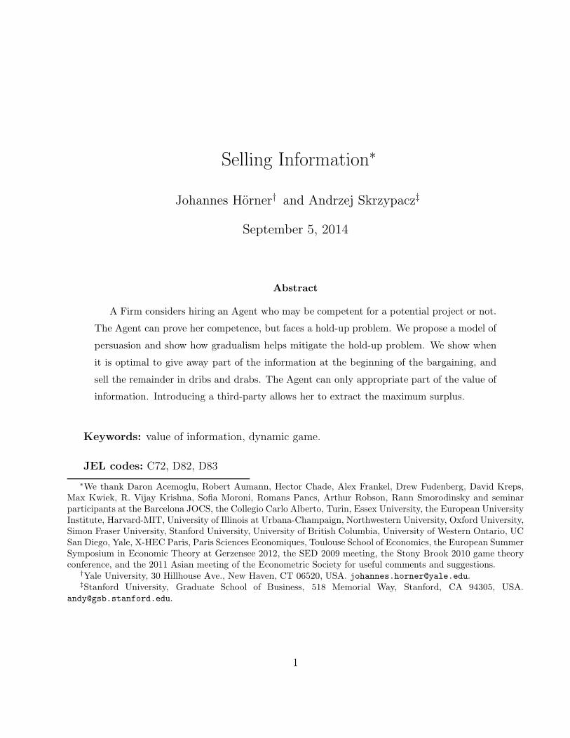
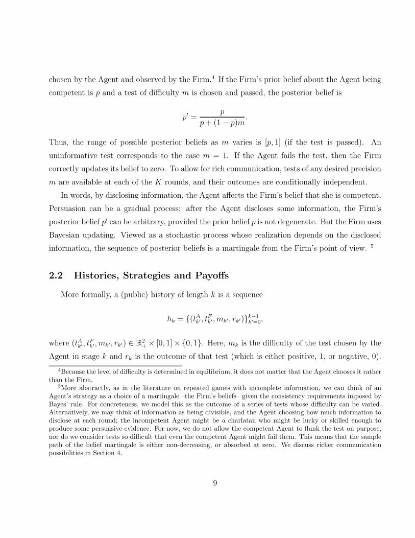
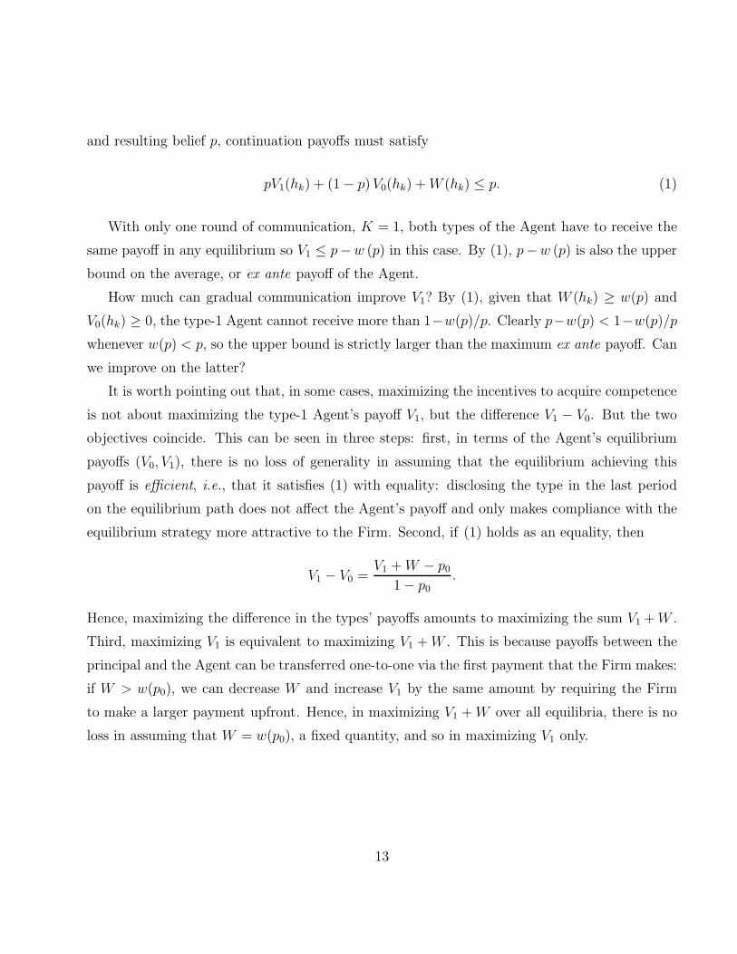
p0 p0 p∗ p′ 1
Figure 1: A feasible action
2.4 The Best Equilibrium for the Competent Agent
We now turn to the focus of the analysis: what equilibrium maximizes the payoff of the
competent Agent, and how much of the surplus can she appropriate? Note that this maximum
payoff is non-decreasing in K, the number of rounds: players can always choose not to make
transfers or disclose any information in the first round. Hence, for any p0, the highest equilibrium
payoff for the type-1 Agent has a well-defined limit as K → ∞ that we seek to identify.
In this and the next section we consider equilibria in which the competent Agent always
passes any test she takes. She is not allowed to “flunk” the test on purpose, a possibility that we
will allow in Section 4: there we enrich the description of the game to allow the agent to choose
whether to pass the test after she chooses the difficulty m. In that richer game the analysis in
this section is equivalent to restricting attention to pure strategies (a restriction that we recall
in formal statements).
From the Firm’s point of view, its posterior will take one of two values: either it jumps from
p0 up to some p′, if the test is successful. Or it jumps down to zero. This is illustrated in Figure
1. The two arrows indicate the two possible posterior beliefs. As mentioned, viewed from the
Firm’s perspective, this belief must follow a martingale: the Firm’s expectation of its posterior
belief must be equal to its prior belief. This is not the case from the Agent’s point of view. Given
her knowledge of the type, she assigns different probabilities to these posterior beliefs than the
Firm. If she is competent, she knows for sure that the belief will not decrease over time. If she
is incompetent, the expectation of the posterior belief is below p0, as she does not know whether
she will be lucky in taking the test (the process is then a supermartingale).
14
Instead of describing the information part of an equilibrium outcome by the tests taken so far
mk and their results, we can equivalently describe it by martingale splitting, i.e. the sequence
of Firm’s beliefs that the type is 1, conditional on all tests so far. As long as the Agent passes the
tests, the Firm’s equilibrium beliefs follow a non-decreasing sequence p0, . . . , pK+1 starting at
the Firm’s prior belief, p0, and ending at pK+1 = 1 (assuming, without loss, that the equilibrium
is efficient). If the Agent fails a test, the posterior drops to zero.
An equilibrium must also specify payments. It turns out that the type-1 Agent’s payoff
decreases if the Firm is ever granted any payoff in excess of its outside option. On the one hand,
the Agent could demand more in earlier rounds by promising to leave some surplus to the Firm
in later rounds. On the other hand, the willingness-to-pay of the Firm for this future surplus is
lower than the cost of such a promise to the type-1 Agent. The reason is that the Firm assigns
a lower probability than the type-1 Agent to the posterior increasing (and payments once the
posterior drops to zero are not individually rational). Finally, it is not hard to see that there is
no point here in having the Agent make any payments. To sum up, if the Firm’s belief in the
next round is either pk+1 or 0, given the current belief pk, then the equilibrium specifies that the
Firm pays her willingness-to-pay
EF [w(p′)]− w(pk),
where p′ is the (random) belief in the next round, with possible values 0 and pk+1, and EF [·] isthe expectation operator for the Firm.
This leaves us with the determination of the sequence of posterior beliefs.7
2.4.1 A Geometric Analysis
We already know that it is possible for the Agent to appropriate some of the value of her
information, but the question is whether she can get more than p0−w(p0), which is just as much
as the type-0 Agent gets in the equilibrium we constructed so far.
Consider first the case K = 1. In this case, the highest equilibrium payoff to the type-1 Agent
7In addition, an equilibrium must also specify how players behave off the equilibrium path. As discussed, themost effective punishment for deviations is reversion to the babbling equilibrium, and this is assumed throughoutunless mentioned otherwise.
15
is indeed equal to p0−w(p0). Suppose that a successful test takes the posterior to p1 ≥ p0. Using
the martingale property, it must be that the probability that the posterior is p1 is p0/p1, because
p0 =p0p1
· p1 +p1 − p0
p1· 0.
hence, the Firm is willing to pay
EF [w(p′)]− w(p0) =
p0p1w (p1)− w (p0) ≤ p0 − w (p0) ,
where the inequality follows from w(p1) ≤ p1. Setting p1 to 1 is best, as it makes the inequality
tight: with one round, revealing all information is optimal.
Note that, when p0 ≤ p∗, w(p0) = 0, and the highest payoff in one round that the type-1
Agent can achieve is the prior p0, which is increasing in p0 ≤ p∗. This suggests one way to
improve on the payoff with two rounds. In the first round, the Agent takes a test whose success
leads to a posterior of p∗ for free. Indeed, the Firm is not willing to pay for a test that does not
affect its outside option. In the second round, the equilibrium of the one-round game is played,
given the belief p∗. This second and only payment yields
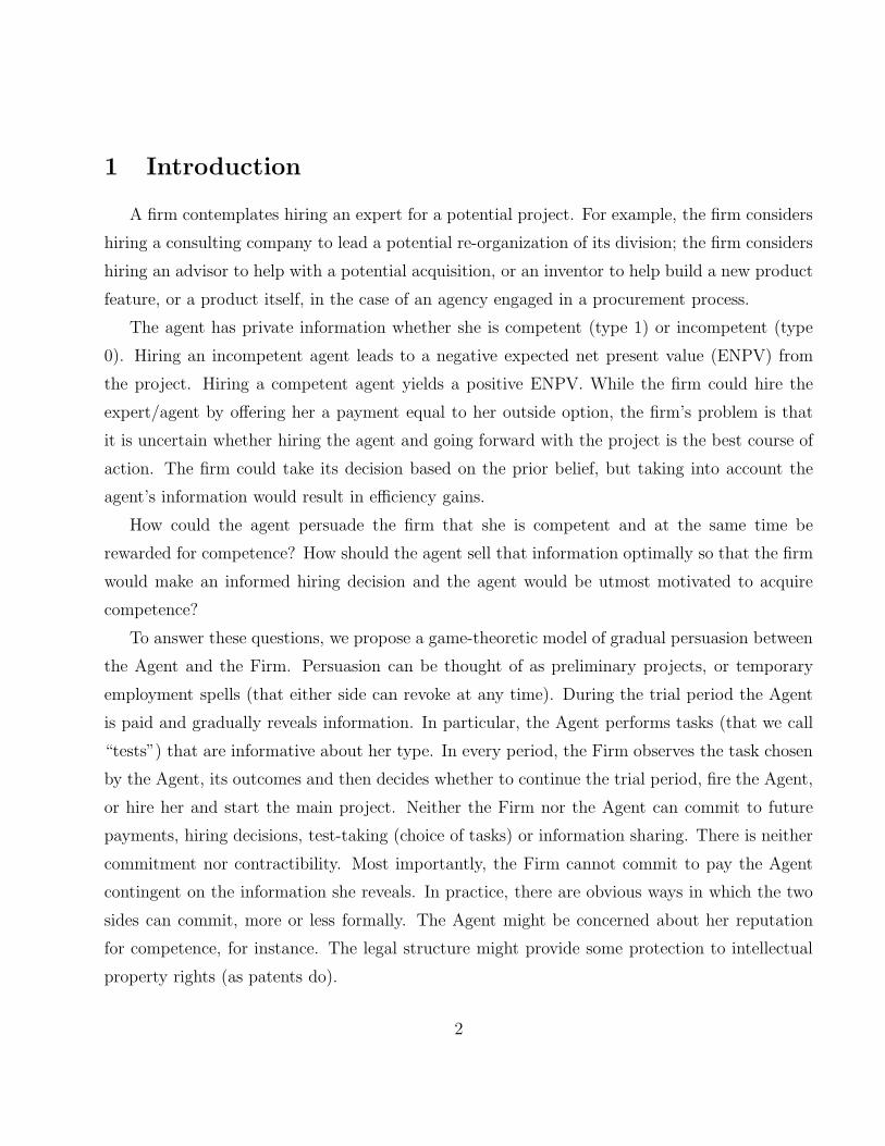
p∗ − w(p∗) = p∗ > p0.
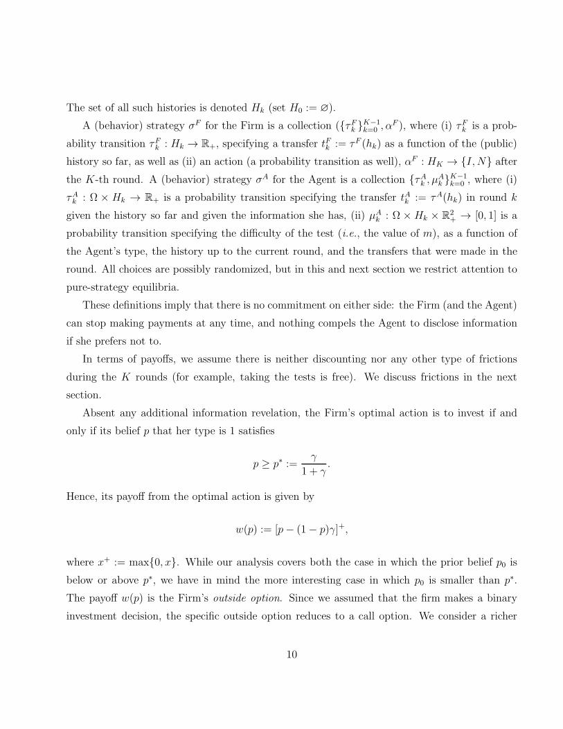
This is illustrated in the right panel of Figure 2. The lower kinked line is the outside option w,
the upper straight line is total surplus, p. Hence, the payment in the second round is given by
the length of the vertical segment at p∗ in the right panel, which is larger than the payment with
only one round, given by the length of the vertical segment at p0.
To sum up: the Agent gives away a chunk of information for free, making the Firm really
unsure whether investing is a good idea. Then she charges as much as she can for the disclosure
of all her information.
Is the splitting that we described optimal with two periods to go? As it turns out, it is so if
and only if p0 < (p∗)2. But there are many other ways of splitting information with two periods
to go that improve upon the one-round equilibrium, and among them, splits that also improve
16
p0 p0 p∗ 1 0 p1
1
$
p0 p∗b
b
b
b
Figure 2: Revealing information in two steps
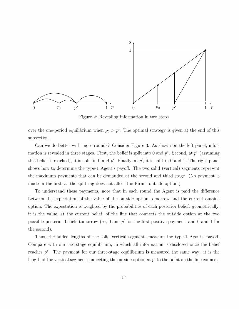
over the one-period equilibrium when p0 > p∗. The optimal strategy is given at the end of this
subsection.
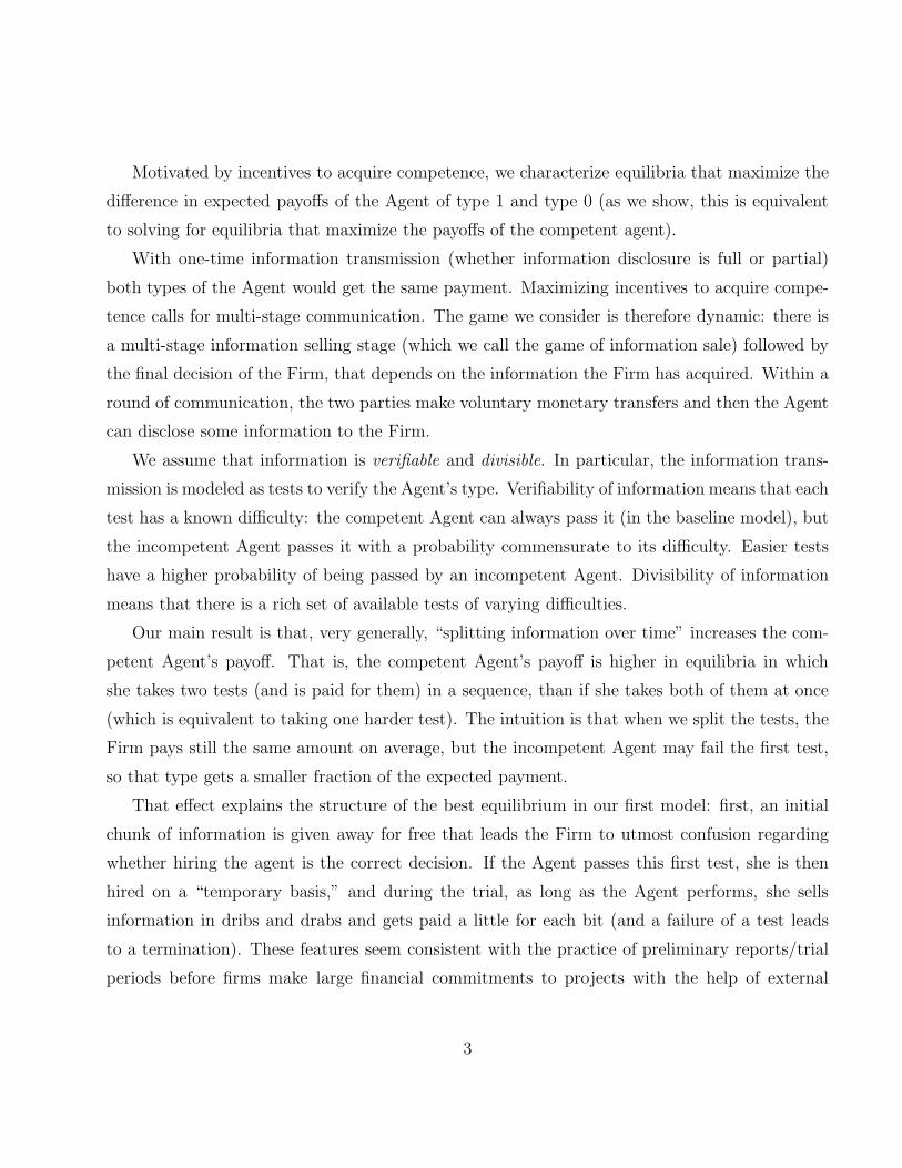
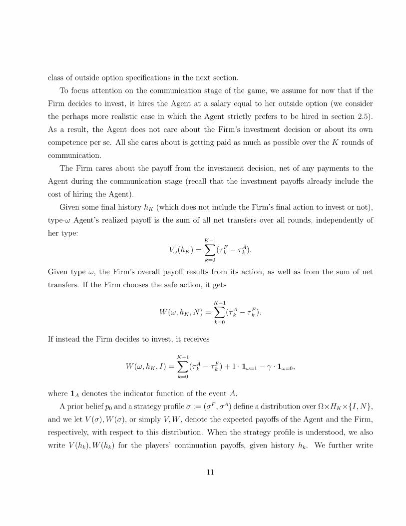
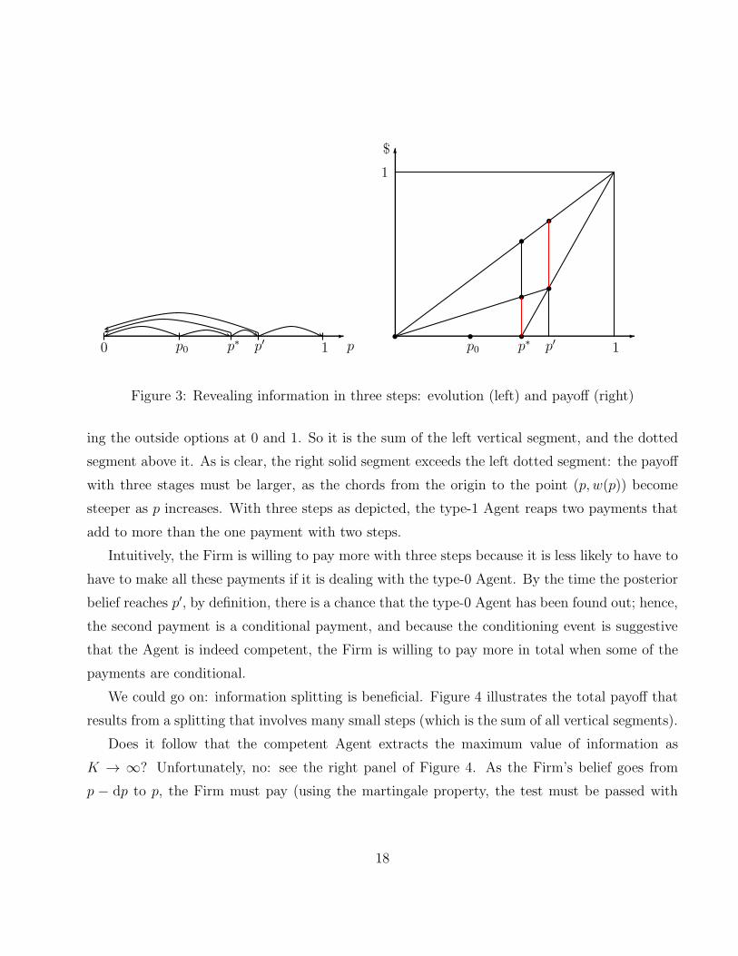
Can we do better with more rounds? Consider Figure 3. As shown on the left panel, infor-
mation is revealed in three stages. First, the belief is split into 0 and p∗. Second, at p∗ (assuming
this belief is reached), it is split in 0 and p′. Finally, at p′, it is split in 0 and 1. The right panel
shows how to determine the type-1 Agent’s payoff. The two solid (vertical) segments represent
the maximum payments that can be demanded at the second and third stage. (No payment is
made in the first, as the splitting does not affect the Firm’s outside option.)
To understand these payments, note that in each round the Agent is paid the difference
between the expectation of the value of the outside option tomorrow and the current outside
option. The expectation is weighted by the probabilities of each posterior belief: geometrically,
it is the value, at the current belief, of the line that connects the outside option at the two
possible posterior beliefs tomorrow (so, 0 and p′ for the first positive payment, and 0 and 1 for
the second).
Thus, the added lengths of the solid vertical segments measure the type-1 Agent’s payoff.
Compare with our two-stage equilibrium, in which all information is disclosed once the belief
reaches p∗. The payment for our three-stage equilibrium is measured the same way: it is the
length of the vertical segment connecting the outside option at p′ to the point on the line connect-
17
p0 p0 p∗ p′ 1 1p0 p∗ p′
s s s
s
s
s
s
$
1
Figure 3: Revealing information in three steps: evolution (left) and payoff (right)
ing the outside options at 0 and 1. So it is the sum of the left vertical segment, and the dotted
segment above it. As is clear, the right solid segment exceeds the left dotted segment: the payoff
with three stages must be larger, as the chords from the origin to the point (p, w(p)) become
steeper as p increases. With three steps as depicted, the type-1 Agent reaps two payments that
add to more than the one payment with two steps.
Intuitively, the Firm is willing to pay more with three steps because it is less likely to have to
have to make all these payments if it is dealing with the type-0 Agent. By the time the posterior
belief reaches p′, by definition, there is a chance that the type-0 Agent has been found out; hence,
the second payment is a conditional payment, and because the conditioning event is suggestive
that the Agent is indeed competent, the Firm is willing to pay more in total when some of the
payments are conditional.
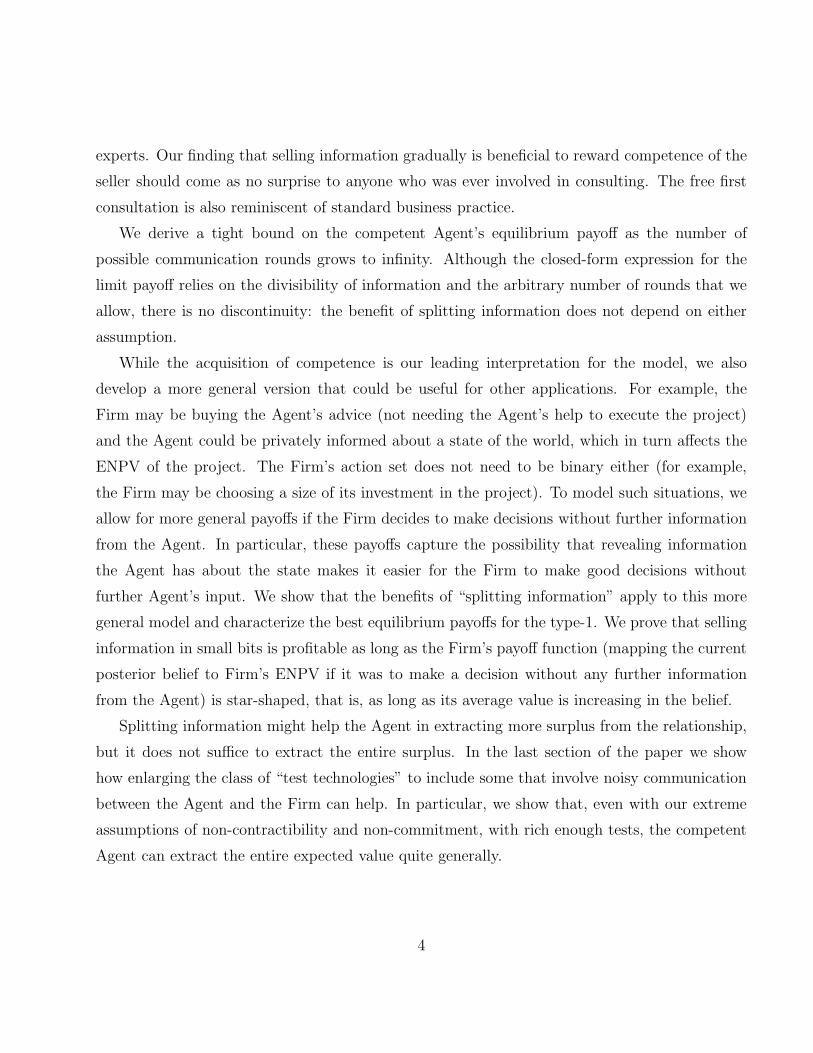
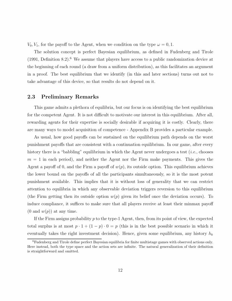
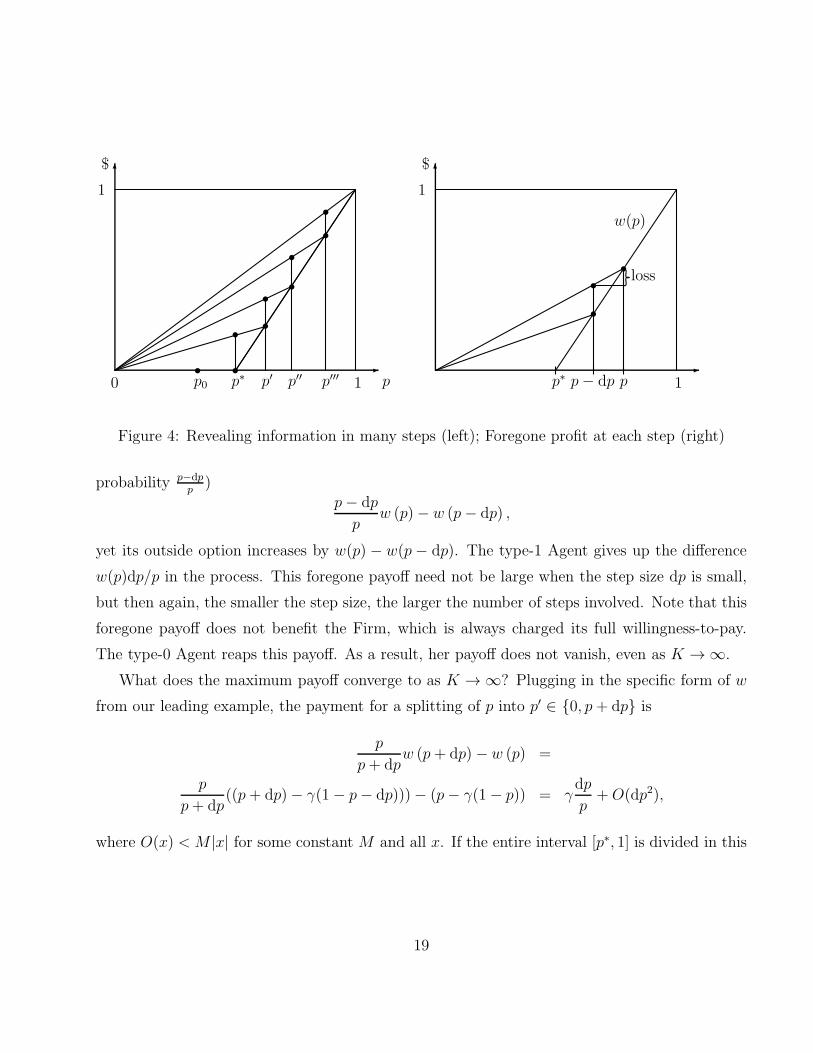
We could go on: information splitting is beneficial. Figure 4 illustrates the total payoff that
results from a splitting that involves many small steps (which is the sum of all vertical segments).
Does it follow that the competent Agent extracts the maximum value of information as
K → ∞? Unfortunately, no: see the right panel of Figure 4. As the Firm’s belief goes from
p − dp to p, the Firm must pay (using the martingale property, the test must be passed with
18
p0 p0 p∗ p′ p′′ p′′′ 1 1p− dpp∗ p
ss
s
s
s
s
s
s
s
1 1
s
s
s
$ $
w(p)
loss
Figure 4: Revealing information in many steps (left); Foregone profit at each step (right)
probability p−dpp
)p− dp
pw (p)− w (p− dp) ,
yet its outside option increases by w(p) − w(p− dp). The type-1 Agent gives up the difference
w(p)dp/p in the process. This foregone payoff need not be large when the step size dp is small,
but then again, the smaller the step size, the larger the number of steps involved. Note that this
foregone payoff does not benefit the Firm, which is always charged its full willingness-to-pay.
The type-0 Agent reaps this payoff. As a result, her payoff does not vanish, even as K → ∞.
What does the maximum payoff converge to as K → ∞? Plugging in the specific form of w
from our leading example, the payment for a splitting of p into p′ ∈ 0, p+ dp is
p
p+ dpw (p+ dp)− w (p) =
p
p+ dp((p+ dp)− γ(1− p− dp)))− (p− γ(1− p)) = γ
dp
p+O(dp2),
where O(x) < M |x| for some constant M and all x. If the entire interval [p∗, 1] is divided in this
19
fashion into smaller and smaller intervals, the resulting payoff to the competent Agent tends to
∫ 1
p∗γdp
p= γ(ln 1− ln p∗) = −γ ln p∗.
This suggests that the limiting payoff is independent of the exact way in which information
(above p∗) is divided up over time, as long as the mesh of the partition tends to zero.
p0 p0 p∗
0.0 0.2 0.4 0.6 0.8 1.0p0.0
0.1
0.2
0.3
0.4
0.5
0.6
0.7
V
V1
V2
V3
V10
V¥
Figure 5: Revealing information in many steps (left); Payoff as a function of K (right).
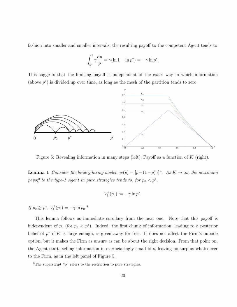
Lemma 1 Consider the binary-hiring model: w(p) = [p−(1−p)γ]+. As K → ∞, the maximum
payoff to the type-1 Agent in pure strategies tends to, for p0 < p∗,
V p1 (p0) := −γ ln p∗.
If p0 ≥ p∗, V p1 (p0) = −γ ln p0.
8
This lemma follows as immediate corollary from the next one. Note that this payoff is
independent of p0 (for p0 < p∗). Indeed, the first chunk of information, leading to a posterior
belief of p∗ if K is large enough, is given away for free. It does not affect the Firm’s outside
option, but it makes the Firm as unsure as can be about the right decision. From that point on,
the Agent starts selling information in excruciatingly small bits, leaving no surplus whatsoever
to the Firm, as in the left panel of Figure 5.
8The superscript “p” refers to the restriction to pure strategies.
20
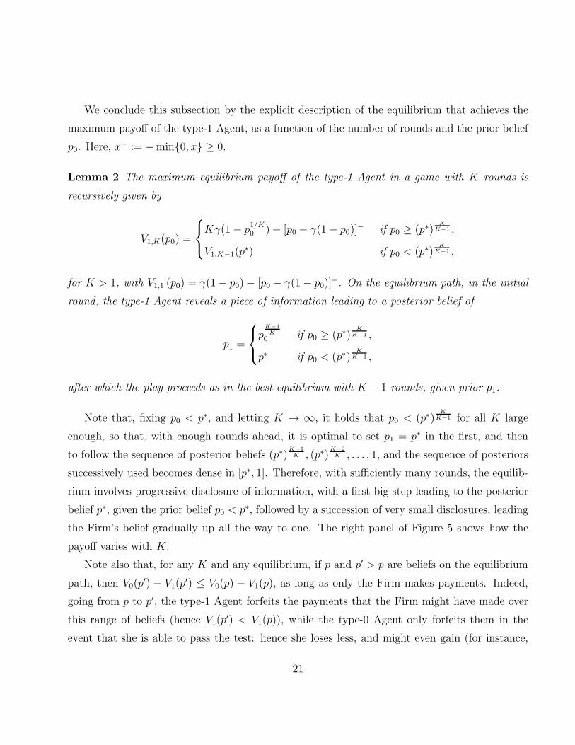
We conclude this subsection by the explicit description of the equilibrium that achieves the
maximum payoff of the type-1 Agent, as a function of the number of rounds and the prior belief
p0. Here, x− := −min0, x ≥ 0.
Lemma 2 The maximum equilibrium payoff of the type-1 Agent in a game with K rounds is
recursively given by
V1,K(p0) =
Kγ(1− p1/K0 )− [p0 − γ(1− p0)]
− if p0 ≥ (p∗)K
K−1 ,
V1,K−1(p∗) if p0 < (p∗)
K
K−1 ,
for K > 1, with V1,1 (p0) = γ(1− p0)− [p0 − γ(1− p0)]−. On the equilibrium path, in the initial
round, the type-1 Agent reveals a piece of information leading to a posterior belief of
p1 =
pK−1K
0 if p0 ≥ (p∗)K
K−1 ,
p∗ if p0 < (p∗)K
K−1 ,
after which the play proceeds as in the best equilibrium with K − 1 rounds, given prior p1.
Note that, fixing p0 < p∗, and letting K → ∞, it holds that p0 < (p∗)K
K−1 for all K large
enough, so that, with enough rounds ahead, it is optimal to set p1 = p∗ in the first, and then
to follow the sequence of posterior beliefs (p∗)K−1K , (p∗)
K−2K , . . . , 1, and the sequence of posteriors
successively used becomes dense in [p∗, 1]. Therefore, with sufficiently many rounds, the equilib-
rium involves progressive disclosure of information, with a first big step leading to the posterior
belief p∗, given the prior belief p0 < p∗, followed by a succession of very small disclosures, leading
the Firm’s belief gradually up all the way to one. The right panel of Figure 5 shows how the
payoff varies with K.
Note also that, for any K and any equilibrium, if p and p′ > p are beliefs on the equilibrium
path, then V0(p′) − V1(p
′) ≤ V0(p) − V1(p), as long as only the Firm makes payments. Indeed,
going from p to p′, the type-1 Agent forfeits the payments that the Firm might have made over
this range of beliefs (hence V1(p′) < V1(p)), while the type-0 Agent only forfeits them in the
event that she is able to pass the test: hence she loses less, and might even gain (for instance,
21
she might not have been able to pass the first free test at p < p∗). As a result, the type-1 Agent
has a preference for lower beliefs, relative to the type-0 Agent. Having to give away information
is more costly to an Agent who knows that she owns it. This plays an important role once noise
(mixed strategies) are considered.
2.5 Agent Prefers to be Hired
So far, we have assumed that the Firm can hire the Agent at her outside option, so that
the Agent is indifferent whether the Firm hires her or not. A perhaps more realistic assumption
is that the Agent’s compensation is strictly higher than her outside option, so that she strictly
prefers being hired. How does that affect our analysis?
Assume that the Agent’s surplus from employment is smaller than the expected net losses
the firm would incur if it hired an incompetent expert, so that not investing remains the efficient
action if the Agent is incompetent (otherwise, investing would be optimal in both states and
communicating competence would not be important).
In this case the equilibrium that maximizes V1 (or V1− V0) has the same equilibrium path as
described above. The only difference is in the off-path behavior supporting it.
First, in our construction above deviations are punished by a babbling equilibrium. That
means that if p ≥ p∗ and the Agent deviates, the Firm still hires her. When the Agent strictly
prefers being hired, this no longer suffices. Once p is sufficiently high, the incompetent type
would prefer not to take any more tests (even if she gets compensated for them) to avoid the
risk of losing employment. In particular, she would not take the last test in round K that
is fully revealing. To sustain our equilibrium outcome we can use the following continuation
equilibrium: if the Agent ever fails to take the test she is expected to take, the Firm’s belief
about her competence drops to 0, and the babbling equilibrium is then played. This clearly
provides incentives for the Agent to take the prescribed tests.
Second, one may worry that the Firm would not make any payments to the Agent knowing
that she wants to be employed and hence has strict incentives in the last period to reveal enough
information to get employed. This creates no difficulty: our equilibrium calls for the Agent to
take for free a test in the first period so that Firm’s beliefs increase to p∗. After that, it is always
22
a best response for the Firm to hire her. So if the Firm deviates to not paying for future tests,
the deviation to a babbling equilibrium (in which the Agent reveals no more information and is
still hired at the end) remains incentive compatible.
Positive employment surplus has two additional effects on the equilibrium that are worth
pointing out. First, it increases V1−V0, because only the competent Agent captures the employ-
ment surplus. Since our equilibrium is separating, leaving employment surplus to the competent
Agent strengthens incentives for acquisition of competence. Second, one may be worried that
in our original construction the Agent is indifferent between revealing and not revealing the last
piece of information in round K, because some considerations left out of the model might break
this indifference, leading to unraveling. With a positive employment surplus the Agent has strict
incentives to take the last, fully-revealing test, because otherwise the Firm would think that she
must be “hiding something,” and not hire her. At the same time, it does not lead to unraveling
because the strict incentives hold only on the equilibrium path. If the Firm deviates by not
paying for some of the tests, the Agent would still be hired, so it would be rational not take the
last test (the competent Agent would be indifferent and the incompetent Agent strictly prefers
to follow the punishment). For further discussion of robustness see Section 3.1.
2.6 Free Entry
The prior belief p0 plays an important role in the analysis, so it is worth discussing how it
might come about. One natural way of endogenizing it is to explicitly model a prior stage in
which agents must decide on whether to invest in competence, so that the benefit of doing so,
which depends on p0, must equal its cost. As a result, the fraction of agents doing the necessary
investment gives rise to the value of p0 that makes precisely this fraction willing to do so.
More directly, we may assume that there is a unit mass of agents (on the short side of the
market), whose choice is to enter either as incompetent for free, or as competent ones at a cost of
c ∈ (0, 1). There are plenty of equilibria –including one where only incompetent agents enter, and
p0 = 0.9 The best equilibrium from a social point of view is the one maximizing p0; indeed, each
competent agent generates a surplus of 1 at a cost of c. But note that it is not an equilibrium
9A small cost of entering as incompetent would eliminate this equilibrium.
23
for every agent to enter as a competent one, as the resulting belief p0 = 1 would strip them
from any additional rewards from further persuading the Firm of their competence. In the best
equilibrium, both types of agents must enter, and so the constraint V1(p0) − V0(p0) = c must
hold. Maximizing p0 thus means selecting the equilibrium that maximizes the difference V1−V0,
as this is the one for which it is possible to pick the highest p0 satisfying the constraint. This is
precisely the equilibrium that we have characterized.
Hence, the best equilibrium yields a prior belief p0 that solves
V1(p0)− V0(p0) = c,
p0V1(p0) + (1− p0)V0(p0) + w(p0) = p0.
If c ∈ (−γ(1 + (1 + γ) ln p∗),−γ ln p∗), the unique solution has p0 = − c+γ ln p∗
1−c∈ (0, p∗).10 If on
the other hand c ≤ −γ(1+(1+γ) ln p∗), the unique solution lies in (p∗, 1). As one would expect,
a lower cost leads to a higher prior belief that an agent is competent, as it is then cheaper for
them to enter.
3 General Outside Options
Assuming that the outside option is given by a call option, as in our main example, provides
a simple illustration of the benefits of splitting, as well as closed-form expressions. However, the
analysis can be generalized.
Such a generalization has two benefits. First, it clarifies what drives the benefits of splitting
information. Second, it encompasses a broader class of applications. Plainly, there is no reason to
confine ourselves to binary decisions by the Firm. For instance, the Firm might choose between
hiring the agent if it deems it profitable; remaining in an Arm’s length relationship with the
Agent; or stopping the relationship altogether.11 Competence is not a one-dimensional attribute.
Furthermore, the value of hiring a competent expert might rely on more than the competence
itself: it might depend on the feasibility of the firm’s project, on the match between this project
10If c ≥ −γ ln p∗, there is no equilibrium with competent entrants.11We thank a referee for suggesting such a ternary decision, as well as useful variations.
24
and the agent’s expertise. Also, there are cases in which tests can be conducted whose outcome
reveals nothing valuable (as is the case with “zero-knowledge proofs” which could be captured
in our model by taking w (p) equal to 0 for all p < 1 and w (1) = 1). In practice, however, it
is difficult to think of demonstrations (blueprints, prototypes, etc.) that do not involve some
valuable information leakage.
Hence, it makes sense to assume that the firm’s outside option depends on its belief in the
agent’s competence in arbitrary ways. Convexity seems to be a natural property to impose, but
as we show an even weaker condition suffices to generalize our results.
Suppose that the payoff of the Firm (gross of any transfers) as a function of its posterior
belief p after the K rounds is a non-negative continuous function w(p),12 and normalize w(0) = 0,
w (1) = 1. We further assume that w (p) ≤ p, for all p ∈ [0, 1], for otherwise full information
disclosure is not socially desirable. This payoff can be thought as the reduced-form of some
decision problem that the Firm faces, as in our baseline model. In that case, w must be convex,
but since it is a primitive here, we do not assume so.
Recall that the best equilibrium with many rounds called for a first burst of information
released for free (assuming p < p∗), after which information is disclosed in dribs and drabs. One
might wonder whether this is a general phenomenon.
The answer, as it turns out, depends on the shape of the outside option. It is in the interest of
the type-1 Agent to split information as finely as possible for any prior belief p0 if and only if the
function w is (strictly) star-shaped, i.e., if and only if the average, w(p)/p, is a strictly increasing
function of p.13 More generally, if a function is star-shaped on some intervals of beliefs, but not
on others, then information will be sold in small bits at a positive price for beliefs in the former
type of interval, and given away for free as a chunk in the latter. In our main example, w is
not star-shaped on [0, p∗], as the average value w(p)/p is constant (and equal to zero) over this
interval. However, it is star-shaped on [p∗, 1]. Hence our finding.
Let us first consider a star-shaped outside option. If in a given round the Firm’s belief goes
12We may without loss assume w to be non-decreasing.13This condition already appears in the economics literature in the study of risk (see Landsberger and Meilijson,
1990). It is weaker than convexity.
25
from p to either (p+ dp) or 0, the Agent can charge up to
p
p+ dpw(p+ dp)− w(p) = (w′(p)− w(p)/p)dp+O(dp2)
for it.14 Given the Firm’s prior belief p0, the type-1 Agent’s payoff becomes then (in the limit,
as the number of rounds K goes to infinity)
∫ 1
p0
[w′(p)− w(p)/p]dp = w(1)− w(p0)−∫ 1
p0
w(p)dp/p,
which generalizes the formula that we have seen for the special case w(p) = [p − (1 − p)γ]+.15
That is, the type-1 Agent’s payoff is the area between the marginal payoff of the Firm and its
average payoff.
To see that splitting information as finely as possible is best in that case, fix some arbitrary
interval of beliefs [p, p], and consider the alternative strategy under which the posterior belief of
the Firm jumps from p to p, the payment from the Firm to the Agent in that round is given by
p
pw(p)− w(p).
If instead this interval of beliefs is split as finely as is possible, the payoff over this range is
w(p)− w(p)−∫ p
p
w(p)
pdp.
Hence, splitting is better if and only if
1
p− p
∫ p
p
w(p)
pdp ≤ w(p)
p, (2)
14In case w (p) is not differentiable, then w′ (p) is the right-derivative, which is well-defined in case w is star-shaped.
15In our main example, w is (globally) weakly star-shaped: that is, the function p 7→ w(p)/p is only weaklyincreasing. The formula for the maximum payoff in the limit K → ∞ is the same whether there is a jump in thefirst period or not. But for any finite K, splitting information disclosures over the range [p0, p
∗] is suboptimal, asit is a “wasted period,” whose cost only vanishes in the limit.
26
p0 p0 p1 1 1p p
$ $
w(p)w(p)
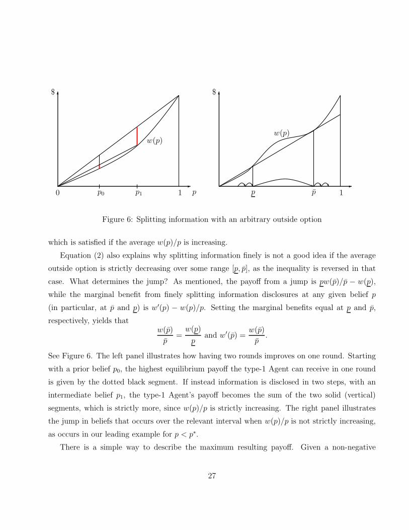
Figure 6: Splitting information with an arbitrary outside option
which is satisfied if the average w(p)/p is increasing.
Equation (2) also explains why splitting information finely is not a good idea if the average
outside option is strictly decreasing over some range [p, p], as the inequality is reversed in that
case. What determines the jump? As mentioned, the payoff from a jump is pw(p)/p − w(p),
while the marginal benefit from finely splitting information disclosures at any given belief p
(in particular, at p and p) is w′(p) − w(p)/p. Setting the marginal benefits equal at p and p,
respectively, yields thatw(p)
p=
w(p)
pand w′(p) =
w(p)
p.
See Figure 6. The left panel illustrates how having two rounds improves on one round. Starting
with a prior belief p0, the highest equilibrium payoff the type-1 Agent can receive in one round
is given by the dotted black segment. If instead information is disclosed in two steps, with an
intermediate belief p1, the type-1 Agent’s payoff becomes the sum of the two solid (vertical)
segments, which is strictly more, since w(p)/p is strictly increasing. The right panel illustrates
the jump in beliefs that occurs over the relevant interval when w(p)/p is not strictly increasing,
as occurs in our leading example for p < p∗.
There is a simple way to describe the maximum resulting payoff. Given a non-negative
27
function f on [0, 1], let
sha f
denote the largest weakly star-shaped function that is smaller than f . In light of the previous
discussion (see right panel of Figure 6), the following result should not be too unexpected.
Theorem 1 The maximum equilibrium payoff to the type-1 Agent in pure strategies tends to, as
K → ∞,
V p1 (p0) = 1− shaw (p0)−
1∫
p0
shaw (p) dp/p,
where p0 := min p ∈ [p0, 1] : w (p) = shaw (p).
That is, the same formula as in the case of a star-shaped function applies, provided one applies
it to the largest weakly star-shaped function that is smaller than w. In words, the maximum
payoff to the type-1 Agent is the area between the marginal and the average outside option of
the Firm, after “regularizing” this outside option by considering the largest weakly star-shaped
function below it.
The proof also elucidates the structure of the optimal information disclosure policy, at least
in the limit. Let
Iw := cl p ∈ [0, 1] : shaw (p) = w (p) and w(p)/p is strictly increasing at p .
In our main example, shaw(p) = w(p) for all p, but Iw = [1/2, 1]. Then the set of on-path beliefs
as K → ∞ held by the firm is contained, and dense, in Iw if Iw 6= ∅. If Iw = ∅, any policy is
optimal.
Note that this result immediately implies that the highest payoff to the type-1 Agent is higher,
the lower the outside option w. That is, if we consider two functions w, w such that w ≥ w,
then the corresponding payoffs satisfy V p1 ≤ V p
1 . The “favorite” outside option for the Agent
is w(p) = 0 for all p < 1, and w(1) = 1 (though this does not quite satisfy our maintained
continuity assumptions). In that case, the type-1 Agent appropriates the entire surplus. This
is the case considered in the literature on “zero-knowledge proofs:” the revision in the Firm’s
28
belief that successive information disclosures entail does not affect its willingness-to-pay.
3.1 Frictions
The only friction assumed so far has been the finiteness of the horizon. Clearly, this is a
simplification. In practice, delaying the action has a cost in terms of discounting. Taking tests
can entails intrinsic costs as well. Finally, the Agent is unlikely to be wholly unconcerned by
the Firm’s action. She might be able to make money out of her information elsewhere; in this
case, she would balk at giving away for free the last bit. Or, to the contrary, she might have a
slight preference for the Firm taking the right action, all else being equal; she would then not
resist giving away this last bit for free if this was the only way to prevent the Firm from making
a mistake. The Firm might then be tempted to forego the payments in hopes that this occurs.
Considering each friction one by one, it is not hard to see that our results are robust to small
perturbations. First, suppose that every additional round of communication is discounted, with
some common discount factor δ ∈ (0, 1). Plainly then, there is no benefit in having arbitrarily
many rounds. This is because the Agent faces a trade-off between collecting more money overall
and collecting it earlier, and because the Firm ultimately prefers taking its outside option rather
than waiting for another period, once the benefits from waiting become small. Hence, in the
best equilibrium, the number of rounds in which communication actually takes place is bounded.
However, as long as the players are not too impatient, the best equilibrium still involves a gradual
release of information. It is easy to see that, as discounting vanishes, the payoff to the competent
Agent must tend to her payoff in the undiscounted game. In Appendix, we prove the following
result.
Lemma 3 Suppose that w is star-shaped and that players discount rounds at rate δ ≥ 1. As
δ → 1, the maximum equilibrium payoff of the type-1 Agent in pure strategies tends to the
undiscounted limit V p1 (p0).
In our main example, it is easy to show that this convergence occurs at a rate that is geometric
in 1− δ.
Suppose now that the horizon is infinite (with low discounting), and introduce a cost to the
Agent taking a test, or transmitting/certifying information. (This is equivalent to each bit of
29
information having an opportunity cost.) Assume that conveying information is socially efficient;
more precisely, assume that the ratio of the cost of taking the posterior belief of the Firm from
p to p′ > p (denoted c(p, p′) ≥ 0) to the benefit p′w(p′)/p− w(p) to the Firm is bounded below
1, uniformly in p, p′.
We can then scale down the information as time passes so as to make sure that the continu-
ation payoff of the two parties incentivizes them to make payments and to take the test.16
In the case of an intrinsic preference of the Agent for the Firm taking either the right or
a given action (worth, say, a given $v(ω, a) ≥ 0, a = I, N , to the Agent, where it is assumed
that incentives are weakly aligned: v(1, I) ≥ v(1, N), v(0, N) ≥ v(0, I)), the procedure must be
modified so that the Agent releases a last chunk of information whose value to the Firm still
exceeds δmaxω,a v(ω, a); if the due payment takes place, the Agent releases this last chunk; if
not, the Agent postpones releasing this information, expecting the Firm to make up for such a
careless slip by making the payment in the next round (if and only if the Agent did not release
this information). See Appendix for a formal proof of the following result.
Lemma 4 Suppose that w is differentiable and star-shaped, and that players discount rounds
at rate δ ≥ 1. Suppose either costs c(p, p′) or intrinsic preferences v(ω, a) as described. As
δ → 1, and either maxp<p′ c(p, p′) → 0 or maxω,a v(ω, a) → 0, the maximum equilibrium payoff
of the type-1 Agent in pure strategies tends to the undiscounted limit (without cost of intrinsic
preferences) V p1 (p0).
We stress that this robustness applies to small perturbations only. Unravelling certainly ap-
plies to our model for certain kinds of perturbations, as it does in related models of contribution
games with irreversibilities (Admati and Perry 1991, Marx and Matthews 2000, etc.). For in-
stance (and this is certainly not the only possibility), if the Agent derives a strictly positive
gain from the Firm taking the right (hiring) decision, and there is a finite horizon, the Firm can
certainly wait until the last period and get all the information for free.
16As usual, one need not think of the information sale phase as lasting literally forever: the low discount factorcan be thought of as a probability of terminating this phase, and it can be generated by the players themselves,using for instance a jointly controlled lottery; in that case, the duration of this phase is (almost surely) finite.
30
4 Noisy Information Transmission
So far, we have assumed that the competent Agent always passes the test, which implies that
the Firm’s posterior belief is either non-decreasing, or absorbed at zero.
There are two reasons why even the competent Agent may fail. First, she may be able to
choose to flunk the test (it turns out that such option may improve upon the equilibria considered
so far). In practice, it is hard to see what prevents an Agent from failing intentionally a given
test: software can be crippled or slowed down, prototypes can be damaged or impaired, imprecise
or even incorrect answers can be given. To model this possibility, we add a third dimension to the
Agent’s strategy; namely, in every round, after a test has been privately performed, the Agent
has the choice, in case of a success, to report a failure. As further notation is not needed, we refer
the interested Reader to the working paper for a formal definition. Because the model considered
in Section 2.4 corresponds to the special case in which the competent Agent always passes the
test –the only interesting pure strategy in the extended model– we refer to this version as the
noisy model. Formally, this is the same model as before, but mixed strategies are considered,
and, as we will see, make a difference.
A second reason for why a competent Agent might fail a test is simply that the test might
be noisy, or very hard. One might devise procedures that are so difficult that even knowledge-
able agents might be occasionally unsuccessful; not many recognized experts provide correct
predictions every time.
There is an important difference between these two cases. In the first case, a competent Agent
who fails the test must be willing to fail. In the second case, she might just not be able to pass
it. Hence, in the first case, equilibrium imposes more stringent requirements than in the second.
Clearly, we can model the second case by allowing for a more general technology, i.e., tests that
are parameterized by two probabilities, (m0, m1), where mω is the probability with which the
type-ω Agent passes the test. From a game-theoretic point of view, this is equivalent to allowing
for a (disinterested) mediator in the baseline model: the competent Agent always passes the test,
whose outcome is observed by the mediator, but not by the Firm. Then, the mediator chooses
whether to report whether the test was successful or not to the Firm. Our description follows
the second approach, and we refer to this version as the model with mediation.
31
While the “game-theoretic” mediator is an abstraction that does not require a third-party
to be involved, but merely the necessary technology (a trustworthy noisy channel whose output
depends on the outcome of the test), it is worth stressing that such intermediaries are actually
being involved in sales of intellectual property. As mentioned in the introduction, there are law
firms, consulting firms and specialized companies that are hired for the purpose of estimating
and certifying the value of intellectual property and facilitating technological transfers.
While noise turns out to be less valuable than mediators, the fundamental principle for why
lower posterior beliefs can be useful is the same in both cases. The next subsection provides an
illustration.
4.1 The Value of Lower Posteriors: An Illustration
Consider the main example, in which the outside option is a simple call option, and consider
γ = 1 and the limiting case K = ∞. Using the best pure-strategy equilibrium (for the type-1
Agent) as a benchmark, the type-1 Agent has a payoff function given by − ln p for p > p∗, and
− ln p∗ for p ≤ p∗.
Suppose that the Firm and the Agent agree to the following (self-enforcing) scheme. If the
test fails, the posterior belief falls to p−∆, for some ∆ > 0. If the test succeeds, the posterior
belief jumps to p + ∆. Pick ∆ such that p∗ < p − ∆ < p + ∆ < 1. Such posterior beliefs are
achieved by mixing by the type-1 Agent (or by a mediator on her behalf), given that the type-0
Agent will disclose that the outcome of the test is a success whenever she is lucky. Because the
possible posterior beliefs are symmetric around p, the two events (that information gets disclosed
or not) must be equally likely from the Firm’s point of view.
The new twist is that, in the event that the posterior belief drops to p − ∆, the Agent is
expected to pay the Firm an amount X > 0. No payment is made by the Agent if the posterior
belief increases to p+∆. Because both posterior beliefs are equally likely, the Firm is willing to
pay X/2 upfront in exchange for this contingent future payment, and the equilibrium calls for
the Firm to make this payment in addition to the familiar term that corresponds to the variation
in its expected outside option.
Such a side-payment is neutral from the point of the view of the Firm: after all, the upfront
32
payment is fair, given the odds that the posterior goes up or down. But it is not fair from
the Agent’s point of view: because the posterior belief is more likely to go down if the Agent
is incompetent, by definition of the posterior belief, this implies that the incompetent Agent is
more likely to have to pay back than the competent Agent. In this fashion, some payoff gets
shifted from the incompetent to the competent Agent.
There are two constraints on the size of this payment X . First, it cannot exceed the con-
tinuation payoff of the type-0 Agent, for otherwise she would renege on the back payment in
case she fails the test. That is, X ≤ V0(p − ∆), where V0 is her continuation payoff. Second,
in the case the mixing is performed by the (type-1) Agent, rather than by a mediator, it must
be that the Agent is actually indifferent between passing or failing the test. In this case, as-
suming that after this payment play resumes according to the best pure strategy equilibrium
described above, the continuation payoffs after this payment are − ln(p + ∆) and − ln(p − ∆)
respectively; hence, we must set X so as to exactly offset this difference in continuation payoffs,
i.e., X = ln(p+∆)− ln(p−∆). This certainly satisfies X < V0(p−∆) if ∆ is small enough. As
mentioned, because V0 − V1 (the difference in payoffs in the best equilibrium) is increasing in p,
this implies that the type-0 Agent is happy to claim she passes the test whenever she is lucky.
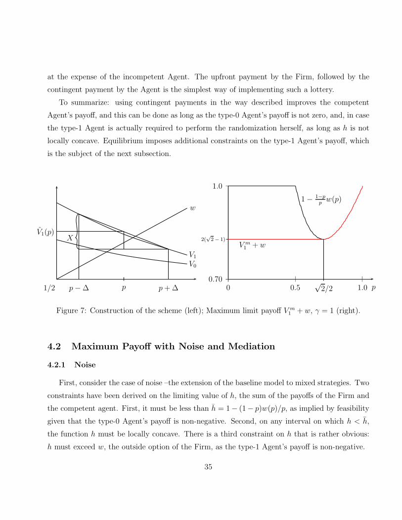
The left panel of Figure 7 illustrates how the mixing works, starting from a given belief p > p∗.
Given that the Firm pays X/2 upfront, and that, by construction, the continuation payoff of
the type-1 Agent is the same whether the posterior belief goes up or down (namely, ln(p−∆)),
her expected payoff is
ln(p+∆)− ln(p−∆)
2+ ln(p−∆) = − ln(p+∆) + ln(p−∆)
2> − ln p,
where the strict inequality follows from Jensen’s inequality. Hence, we have just improved on
our limit payoff V1(p) = − ln p.
What is the key to this improvement, and how much can such schemes improve on the
competent Agent’s payoff? It turns out to depend on the curvature of the sum of the Firm’s
and competent Agent’s payoffs. Let V m0 (p) and V m
1 (p) denote the limiting payoffs as K → ∞in the best equilibrium that uses mixed (or pure) strategies and define h(p) := V m
1 (p) + w(p). if
V m0 (p) = 0 for some p, the incompetent Agent would no longer make any payments; by (1), this
33
implies that h(p) = h(p) := 1− (1− p)w(p)/p (h is the bound from (1) and V0 ≥ 0). This would
yield the highest possible payoff to the competent Agent, given the Firm’s outside option. So
suppose that h < h on some interval around p, and for the sake of contradiction, assume that h
is not concave on this interval, i.e. there exists p1 < p < p2 such that
h(p) <p2 − p
p2 − p1h(p1) +
p− p1p2 − p1
h(p2).
We generalize the previous scheme to this case: the agent pays V m1 (p1)−V m
1 (p2) to the principal
if and only if the posterior drops to p1, and play reverts then (or if the posterior belief turns
out to be p2) to the equilibrium that achieves V m1 . The type-1 Agent is indifferent between both
posterior beliefs, and so is willing to randomize. Given her assessment of the likelihood of each
of these events, the Firm is willing to pay upfront
p2 − p
p2 − p1[w(p1) + V m
1 (p1)− V m1 (p2)] +
p− p1p2 − p1
w(p2)− w(p),
as this is the difference between its expected continuation payoff and its current outside option.
The type-1 Agent’s payoff V1(p) consists then of this payment and her continuation payoff V m1 (p2),
so that, adding up,
h(p) ≥ V1(p) + w(p) =p2 − p
p2 − p1[w(p1) + V m
1 (p1)− V m1 (p2)] +
p− p1p2 − p1
w(p2) + V m1 (p2)
=p2 − p
p2 − p1h(p1) +
p− p1p2 − p1
h(p2).
Note that the participation constraint for the incompetent Agent, V m0 (p1) > V m
1 (p1)−V m1 (p2) is
always satisfied if p1, p2 are close enough to p and V m0 (p1) > 0, and so h must be locally concave
at any p at which V m0 (p) > 0.17
The concavity of the sum of the payoffs of the competent Agent and the Firm in the best
equilibrium should not be surprising: if it were convex, a lottery could increase their joint payoff,
17This hinges on continuity of V m1 and V m
0 ; V m1 is continuous because it is always possible to use the same
disclosure strategy starting at p2 as the continuation strategy given p1 would specify from the first posterior beliefabove p2 onward; the first payment must be adjusted, but the continuity in payoffs as p1 → p2 then follows fromthe continuity of w. Continuity of V m
0 follows from the continuity of V m1 .
34
at the expense of the incompetent Agent. The upfront payment by the Firm, followed by the
contingent payment by the Agent is the simplest way of implementing such a lottery.
To summarize: using contingent payments in the way described improves the competent
Agent’s payoff, and this can be done as long as the type-0 Agent’s payoff is not zero, and, in case
the type-1 Agent is actually required to perform the randomization herself, as long as h is not
locally concave. Equilibrium imposes additional constraints on the type-1 Agent’s payoff, which
is the subject of the next subsection.
1/2
V0
pp−∆ p+∆
V1(p)
V1
X
w
p0.70
1.0
0 0.5 1.0√2/2
V m1 + w
1− 1−ppw(p)
2(√2− 1)
Figure 7: Construction of the scheme (left); Maximum limit payoff V m1 + w, γ = 1 (right).
4.2 Maximum Payoff with Noise and Mediation
4.2.1 Noise
First, consider the case of noise –the extension of the baseline model to mixed strategies. Two
constraints have been derived on the limiting value of h, the sum of the payoffs of the Firm and
the competent agent. First, it must be less than h = 1− (1− p)w(p)/p, as implied by feasibility
given that the type-0 Agent’s payoff is non-negative. Second, on any interval on which h < h,
the function h must be locally concave. There is a third constraint on h that is rather obvious:
h must exceed w, the outside option of the Firm, as the type-1 Agent’s payoff is non-negative.
35

Finally, the basic splitting of Section 2.4 delivers one more restriction, namely, the function h
must be no steeper than w(p)/p. We can always split the prior belief p0 into the posterior beliefs
in 0, p1, p1 > p0. The Firm is willing to pay p0w(p1)/p1 −w(p0) for such a test, so that, at the
very least,
V m1 (p0) ≥
p0p1w(p1)− w(p0) + V m
1 (p1),
orh(p1)− h(p0)
p1 − p0≤ w(p1)
p1. (3)
If h were known to be differentiable, this would reduce to the requirement that h′(p) be smaller
than w(p)/p. More generally, chords connecting points (p0, h(p0)) and (p1, h(p1)) must be flatter
than the ray with slope w(p1)/p1.
We summarize these requirements in the following definition.
Definition 1 Given the outside option w, we define hm : [0, 1] → R+ as the smallest function
such that:
1. For all p, hm ≤ h(p) := 1− (1− p)w(p)/p;
2. If hm < h on [p0, p1], then h is locally concave on [p0, p1].
3. For all p, hm ≥ w(p);
4. For all p1 > p0,hm(p1)− hm(p0)
p1 − p0≤ w(p1)
p1.
As it turns out, equilibrium imposes no additional restriction on h, as we show in Appendix.18
What is the smallest function that satisfies these four requirements?19 In our main example, some
18Roughly, any function satisfying these properties cannot be improved upon with one more round, even withmixed strategies. Because the payoff of the type-1 Agent is increasing in her continuation payoff, this meansthat the highest limiting payoff must be below this function. Conversely, the limiting payoff must satisfy theseproperties. Hence, it follows that this lowest function is the limiting payoff.
19One might wonder why the smallest function h satisfying the requirements is the appropriate one; this isbecause, starting from the highest equilibrium payoff with one round, and applying the two schemes that we havedescribed, we recursively obtain higher values for h as the number of rounds increases, but we cannot “overtake”the smallest function that satisfies the four requirements.
36
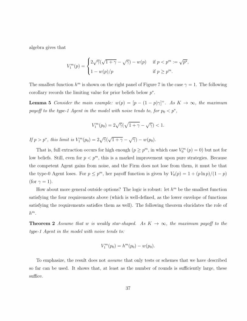
algebra gives that
V m1 (p) =
2√γ(√1 + γ −√
γ)− w(p) if p < pm :=√p∗,
1− w(p)/p if p ≥ pm.
The smallest function hm is shown on the right panel of Figure 7 in the case γ = 1. The following
corollary records the limiting value for prior beliefs below p∗.
Lemma 5 Consider the main example: w(p) = [p − (1 − p)γ]+. As K → ∞, the maximum
payoff to the type-1 Agent in the model with noise tends to, for p0 < p∗,
V m1 (p0) = 2
√γ(√
1 + γ −√γ) < 1.
If p > p∗, this limit is V m1 (p0) = 2
√γ(√1 + γ −√
γ)− w(p0).
That is, full extraction occurs for high enough (p ≥ pm, in which case V m0 (p) = 0) but not for
low beliefs. Still, even for p < pm, this is a marked improvement upon pure strategies. Because
the competent Agent gains from noise, and the Firm does not lose from them, it must be that
the type-0 Agent loses. For p ≤ pm, her payoff function is given by V0(p) = 1 + (p ln p)/(1 − p)
(for γ = 1).
How about more general outside options? The logic is robust: let hm be the smallest function
satisfying the four requirements above (which is well-defined, as the lower envelope of functions
satisfying the requirements satisfies them as well). The following theorem elucidates the role of
hm.
Theorem 2 Assume that w is weakly star-shaped. As K → ∞, the maximum payoff to the
type-1 Agent in the model with noise tends to:
V m1 (p0) = hm(p0)− w(p0).
To emphasize, the result does not assume that only tests or schemes that we have described
so far can be used. It shows that, at least as the number of rounds is sufficiently large, these
suffice.
37
4.2.2 Mediation
It turns out that a similar reasoning can be used to characterize the maximal V1 in case a
mediator can send noisy messages based on the test results (or the Agent has access to noisy
tests). The only difference is that the scheme that involves payments by the Agent in case
the posterior drops is no longer constrained by the indifference of the competent Agent, which
imposed that h was locally concave whenever h fell short of the upper bound h. So we are left
with the other three restrictions on the function h. It turns out, as before, that the solution
is given by the smallest function satisfying these requirements. The maximum payoff has a
particularly simple expression, and the result does not require w to be star-shaped.
As the next theorem states, the type-1 Agent can extract all the surplus from the type-0
Agent as well as the Firm, up to its outside option.
Theorem 3 As K → ∞, the maximum payoff to the type-1 Agent with an intermediary tends
to:
V int1 (p0) = 1− w(p0)
p0.
In our main example, this means that, for p0 < p∗, the maximum payoff of the competent
Agent is 1 –and there is nothing left to improve upon.
5 Final Remarks
This paper describes self-enforcing contracts based on gradual persuasion to facilitate sale
of information. Clearly, in real-life applications, the mechanism that we describe is limited by
the extent to which information is divisible, or tests are available. On the other hand, it can be
facilitated by repeated interactions and reputation-building.
As mentioned in the introduction, our mechanism is reminiscent of zero-knowledge proofs.
But gradualism is a technological constraint in this literature. There is no counterpart to the
Firm’s outside option, and the only objective is to convince the other party that the Agent holds
the information. It is as if w(p) = 0 for p < 1, and w(1) = 1, in which case it is optimal to reveal
all details but the “last key,” increasing the Firm’s posterior close to 1, and then to sell just
38
that remaining piece. Gradualism arises in our mechanism precisely because the Firm’s outside
option depends on its belief, as is plausible in most economic applications. In fact, often the
buyer has private information as well, and an inventor always risks making herself obsolete by
revealing additional information to the Firm. Considering such a model, in which both parties
hold private information, is left for future research.
References
[1] Admati, A.R. and M. Perry (1991). “Joint Projects without Commitment,” The Review of
Economic Studies, 58, 259–276.
[2] Admati, A.R. and P. Pfleiderer (1990). “Direct and Indirect Sale of Information,” Econo-
metrica, 58, 901–928.
[3] Admati, A.R. and P. Pfleiderer (1988). “Selling and Trading on Information in Financial
Markets,” The American Economic Review, P&P, 78, 96–103.
[4] Anton, J. and D. Yao (1994). “Expropriation and Inventions,” The American Economic
Review, 84, 190–209.
[5] Anton, J. and D. Yao (2002). “The Sale of Ideas: Strategic Disclosure, Property Rights, and
Contracting,” The Review of Economic Studies, 69, 513–531.
[6] Aumann, R.J. and S. Hart (2003). “Long Cheap Talk,” Econometrica, 71, 1619–1660.
[7] Aumann, R.J. and M.B. Maschler (1995). Repeated Games with Incomplete Information,
The MIT Press.
[8] Bruckner, A.M. and E. Ostrow (1962). “Some function classes related to the class of convex
functions,” Pacific Journal of Mathematics, 12, 1203–1215.
[9] Che, Y.-K. and J. Sakovics (2004). “A Dynamic Theory of Holdup,” Econometrica, 72,
1063–1103.
39
[10] Compte, O. and P. Jehiel (2004). “Gradualism in Bargaining and Contribution Games,”
The Review of Economic Studies, 71, 975–1000.
[11] Ely, J., A. Frankel and E. Kamenica (2013). “Suspense and Surprise,” Chicago Booth,
working paper.
[12] Eso, P. and B. Szentes (2007). “The price of advice,” The Rand Journal of Economics, 38,
863–1179.
[13] Forges, F. (1990). “Equilibria with Communication in a Job Market Example,” The Quar-
terly Journal of Economics, 105, 375–398.
[14] Forges, F. and F. Koessler (2008). “Long Persuasion Games,” Journal of Economic Theory,
143, 1–35.
[15] Fudenberg, D. and J. Tirole (1991). Game Theory, MIT Press, Cambridge.
[16] Kamenica, E. and M. Gentzkow (2011). “Bayesian Persuasion,” American Economic Review,
101, 2590–2615.
[17] Goldwasser, S., S. Micali and C. Rackoff (1985). “The knowledge complexity of interactive
proof-systems,” In Proc. 17th ACM Symp. on Theory of Computing, Providence, ACM,
291–304.
[18] Gul, F. (2001). “Unobservable Investment and the Hold-Up Problem,” Econometrica, 69,
343–376.
[19] Landsberger, M. and I. Meilijson (1990). “Lotteries, insurance and star-shaped utility func-
tions,” Journal of Economic Theory, 52, 1–17.
[20] Marx, L.M. and S.A. Matthews (2000). “Dynamic Voluntary Contribution to a Public
Project,” The Review of Economic Studies, 67, 327–358.
[21] Matthews, S.A. and A. Postlewaite (1995). “On Modeling Cheap Talk in Bayesian Games,”
in The Economics of Informational Decentralization: Complexity, Efficiency, and Stability:
Essays in Honor of Stanley Reiter, ed. J.O. Ledyard, Kluwer Academic Publishers, 347–366.
40
[22] Rosenberg, D., Solan, E. and N. Vieille (2013). “Strategic Information Exchange,” Games
and Economic Behavior, 82, 444–467.
[23] Spence, M. (1973). “Job Market Signaling,” Quarterly Journal of Economics, 87, 355–374.
A Proofs
Because mediation imposes one fewer constraints on the payoff function to be determined
than noise, as explained in Section 4.2.2, we prove the three theorems in the following order:
first, Theorem 1 (pure strategies), then Theorem 3 (mediation) and then Theorem 2 (noise).
A.1 Proof of Lemma 2 and Lemma 1
The proof of Lemma 2 is by induction on the number of rounds. Lemma 2 immediately
implies Lemma 1.
Our induction hypothesis is that, with k ≥ 1 periods to go, and a prior belief p = p0, the
best equilibrium involves setting the next (non-zero) posterior belief, p1, equal to p1 = pk−1k if
pk−1k ≥ p∗ (i.e. if p ≥ (p∗)
k
k−1 for k ≥ 2), and equal to p∗ otherwise.20 Further, the type-1 Agent’s
maximal payoff with k rounds to go is equal to
V1,k(p) = kγ(1− p1/k)− [p− γ(1− p)]− if p ≥ (p∗)k
k−1 , and V1,k(p) = V1,k−1(p∗) if p < (p∗)
k
k−1 .
Note that this claim implies that V1,k(p∗) = kγ
(
1− (p∗)1/k)
. Finally, as part of our induction
hypothesis, we claim the following. Given some equilibrium, let X ≥ 0 denote the payoff of the
Firm, net of its outside option, with k rounds left. That is, X := Wk(p)− w(p), where Wk(p) is
the Firm’s payoff given the history leading to the equilibrium belief p with k rounds to go. Let
V1,k(p,X) be the maximal payoff of the type-1 Agent over all such equilibria, with associated
belief p, and excess payoff X promised to the Firm (set V1,k(p,X) := −∞ if no such equilibrium
exists). Then we claim that V1,k(p,X) ≤ V1,k(p)−X. We first verify this with one round. Clearly,
20In this proof, when we say that the equilibrium involves setting the posterior belief p1, we mean that, fromthe type-1 Agent’s point of view, the posterior belief will be p1, while from the point of view of the Firm, theposterior belief will be a random variable p′ with possible values 0, p1 .
41
if K = 1, it is optimal to set the posterior p1 equal to 1, which is pK−1K , the relevant specification
given that p01 = 1 ≥ p∗. The payoff to the type-1 Agent is
V1,1 (p) = p− [p− γ(1− p)]+ = γ(1− p)− [p− γ(1− p)]−,
as was to be shown. Note that this equilibrium is efficient. This implies that V1,1(p,X) ≤V1,1(p)−X, for all X ≥ 0, because any additional payoff to the Firm must come as a reduction
of the net transfer from the Firm to the Agent.
Assume that this holds with k rounds to go, and consider the problem with k + 1 rounds.
Of course, we do not know (yet) whether, in the continuation game, the Firm will be held to its
outside option.
Note that the Firm assigns probability p/p1 to the event that its posterior belief p′ will be
p1, because, by the martingale property, we have
p = EF [p′] =
p
p1· p1 +
p1 − p
p1· 0.
This implies that, with k+1 rounds, the Firm is willing to pay at most tFk+1 :=pp1(w (p1) +X ′)−
w (p) , where X ′ is the excess payoff of the Firm with k rounds to go, given posterior belief p1.
Therefore, the payoff to the type-1 Agent is at most
V1,k+1(p) ≤ tFk+1 + V1,k(p1;X′) ≤ p
p1(w (p1) +X ′)− w(p) + V1,k(p1)−X ′,
where the second inequality follows from our induction hypothesis. Note that, since p/p1 < 1,
this is a decreasing function of X ′: it is best to hold the Firm to its outside option when
the next round begins. Therefore, we maximize pp1w (p1) + V1,k(p1). Note first that, given the
induction hypothesis, all values p1 ∈ [p, (p∗)k
k−1 ) yield the same payoff, because for any such p1,
V1,k(p1) = V1,k−1(p∗). The remaining analysis is now a simple matter of algebra. Note that, for
p1 ∈ [(p∗)k
k−1 , p∗) (which obviously requires p < p∗), the objective becomes (using the induction
hypothesis)
V1,k(p1) = kγ(1− (p1)1/k)− (p1 − γ(1− p1))
−,
42
which is increasing in p1, so that the only candidate value for p1 in this interval is p1 = p∗.
Consider now picking p1 ≥ p∗. Then we maximize
p
p1(p1 − γ(1− p1)) + kγ(1− p
1/k1 ),
which admits a unique critical point p1 = pk
k+1 , achieving a payoff equal to (k+1)γ(1−p1/(k+1))+
p− γ(1 − p) = (k + 1)γ(1 − p1/(k+1)). Note, however, that this critical point satisfies p1 ≥ p∗ if
and only if p ≥ (p∗)k+1k .
Therefore, the unique candidates for p1 are p∗,maxp∗, p k
k+1, 1. Observe that setting the
posterior belief p1 equal to maxp∗, p k
k+1 does at least as well as choosing either p∗ or 1. This
establishes the optimality of the strategy, and the optimal payoff for the type-1 Agent, with k+1
rounds to go.
Finally, we must verify that V1,k+1(p;X) ≤ V1,k+1(p)−X . Given that we have observed that
it is optimal to set X ′ = 0 in any case, any excess payoff to the Firm with k + 1 rounds to go is
best obtained by a commensurate reduction in the net transfer from the Firm to the Agent in the
first round (among the k+ 1 rounds). This might violate individual rationality for some type of
the Agent, but even if it does not, it still yields a payoff V1,k+1(p;X) no larger than V1,k+1(p)−X
(if it does violate individual rationality, V1,k+1(p;X) must be lower).
A.2 Proof of Theorem 1
Given a function f , the average function of f is denoted
fa (x) := f (x) /x.
Given a non-negative functionf on [0, 1], let sha f denote the largest weakly star-shaped function
that is smaller than f . This function is well-defined, because (i) if f1, f2 are two weakly star-
shaped functions lower than f , the pointwise maximum g (i.e. g(p) := maxf1(p), f2(p)) is
star-shaped as well,21 and (ii) the limit of a convergent sequence of star-shaped functions is star-
21Given p1 < p2 , let g(p1) = fi(p1), g(p2) = fj(p2). Then ga(p2) = faj (p2) ≥ fa
i (p2) ≥ fai (p1) = ga(p1).
43
shaped (Thm. 2, Bruckner and Ostrow, 1962), who also show that a non-negative star-shaped
function (with w(0) = 0) must be non-decreasing.
The theorem claims that the equilibrium payoff, given w, and w := shaw, is given by
V p1 (p0) = 1− w (p0)−
1∫
p0
wa (p) dp,
where p0 := min p ∈ [p0, 1] : w (p) = shaw (p). Further, letting
Iw = cl p ∈ [0, 1] : shaw (p) = w (p) and wa is strictly increasing at p ,
we show that the set of beliefs held by the firm is contained, and dense, in Iw if Iw 6= ∅. If
Iw = ∅, any policy is optimal.
Let us start by showing that this payoff can be achieved asymptotically (i.e., asK → ∞). Let
Jw denote the complement of Iw, which is a union of disjoint open intervals. Let (p−n , p+n )n∈Ndenote an enumeration of its endpoints. Finally, let p0 := min p ∈ Iw, p ≥ p0. Note that, for
all n, by continuity of w(using that w(p+n )
p+n= w(p−n )
p−nby definition of (p−n , p
+n )),
w(
p+n)
− w(
p−n)
−p+n∫
p−n
wa (p) dp = p−n(
wa(
p+n)
− wa(
p−n))
= 0.
Similarly, if p0 < p0,
w (p0)− w (p0)−p0∫
p0
wa (p) dp = 0.
Fix any sequence of finite subsets of points PK =
pKk : k = 0, . . . , K
⊆ Iw ∩ [p0, 1] (where
pKk is strictly increasing in k), for K ∈ N, with pK0 = p0, pKK = 1, such that pK becomes dense
in Iw as K → ∞. Consider the pure strategy according to which, in the first period, if p0 > p0,
the type-1 Agent gives away the information for free that leads to a posterior p0; afterwards, the
price paid in each period given that the posterior is supposed to move from pKk to pKk+1 is given by
44
the maximum amount pKk(
wa(
pKk+1
)
− wa(
pKk))
. Failure to pay leads to no further disclosure,
and failure to disclose leads to no further payment. Given K, the payoff of following this pure
strategy is (by considering Riemann sums and using the equality from the previous equation)
K−1∑
k=0
pKk(
wa(
pKk+1
)
− wa(
pKk))
→ 1− w (p0)−∫
Iw∩[p0,1]wa (p) dp = 1− w (p0)−
1∫
p0
wa (p) dp.
Conversely, we show that (i) for any K, the best payoff given w is the same as for some
weakly star-shaped function smaller than w, and (ii) if w ≥ w, then V1 ≤ V1. The result follows.
Note that the payoff from the sequence of beliefs p1, p2, . . . , pK−1, pK = 1, starting from p0 is
given by
p0(wa(p1)− wa(p0)) + p1(w
a(p2)− wa(p1)) + · · ·+ pK−1 · (wa(1)− wa(pK−1))
= 1− w(p0)− (1− pK−1)wa(1)− · · · − (p1 − p0)w
a(p1),
so that
V1,K(p0) + w(p0) = 1−K−1∑
k=0
(pk+1 − pk)wa(pk+1).
Note that maximizing V1,K(p) +w(p) and maximizing V1,K(p) are equivalent, so this amounts to
finding the sequence that maximizes the sum
1−K−1∑
k=0
(pk+1 − pk)wa(pk+1),
with p0 = p. Because w ≤ w implies wa ≤ wa, we have just established the following.
Lemma 6 Suppose that w ≥ w pointwise. Then, for every K, and every prior belief p0,
V1,K(p0) ≤ V1,K(p0),
where V1,K(p0) and V1,K(p0) are the type-1 Agent’s payoffs given outside option w and w, respec-
tively.
45
To every sequence of beliefs p0, p1, . . . , pK = 1, we can associate the piecewise linear function wK
on [p0, 1] that obtains from linear interpolation given the points
(p0, w(p0)), (p1, w(p1)), . . . , (1, 1).
Lemma 7 For all K, p0, the optimal policy is such that the function wK is weakly star-shaped.
Proof: This follows immediately from the payoff from the formula for the price of a jump from
p1 to p2,
p1 (wa (p2)− wa (p1)) .
Indeed, if p1, p2, p3 are consecutive jumps, it must be that doing so dominates skipping p2, i.e.
p1 (wa (p2)− wa (p1)) + p2 (w
a (p3)− wa (p2)) ≥ p1 (wa (p3)− wa (p1)) ,
or wa(p3) ≥ wa(p1). A similar argument applies to the first jump.
Note finally that the payoff from the sequence p1, . . . , pK given w is the same as given wK .
The result follows. The asymptotic properties of the optimal policy follow as well.
We start with the theorem, which implies the lemma by a straightforward computation.
A.3 Proof of Lemma 3
When there is discounting, the payment made when the current belief is p and the next belief
is p′ > p (or 0) is given by
t(p) =p
p′w(p′)− w(p).
Here, for simplicity, we assume that the function w is strongly star-shaped on the relevant interval
of beliefs [p0, 1], that is, there exists ν > 0 such that, for all p ∈ [p0, 1], pw′(p)− w(p) > ν. If as
in our main example the function is star-shaped, but not strongly star-shaped, given the prior
(it is strongly star-shaped if p0 > p∗), an elementary adaptation is required (e.g., in the main
example, if the prior p is lower than p < p∗, give for free a piece of information such that the
posterior p1 is strictly above, but arbitrarily close to p∗, and follow then the same argument.)
46

Fix the prior p0 > 0. We consider a strategy in which p/p′ is kept constant in all but a final
period of disclosure. That is, assume that p′ = (1 + k)p, for some k > 0 (and all p < 1/(1 + k)).
Once (1 + k)p > 1 given p, information is disclosed in one shot (for the maximum price).
We set k =√1− δ. The assumption that w is strongly star-shaped ensures that there exists
δ < 1, for all δ ∈ (δ, 1), and all p ∈ [p0, 1/(1 +√1− δ)],
δp′
pw(p′)− w(p) =
δ
1 +√1− δ
w((1 +√1− δ)p)− w(p) > 0.
We write p(0) = p0, p(n) = (1 + k)np0, and compute the value function V from this policy:
V (p0) =δ
1 + kw(p(1))− w(p) + δV (p(1))
=δw(p(1))
1 + k− w(p) + δ
(
δw(p(2))
1 + k− w(p(1))
)
+ · · ·+ δT(
δw(p(T+1))
1 + k− w(p(T ))
)
,
where T is the number of steps until the belief 1/(1 +√1− δ) is exceeded, that is, T = maxt :
(1 + k)tp ≤ 1/(1 +√1− δ). Alternatively, T = ⌊− ln((1+
√1−δ)p)
ln(1+k)⌋. Rearranging,
V (p0) =δT+1
1 + kw(p(T+1))− w(p)− δ
k
1 + kw(p(1))− · · · − δT
k
1 + kw(p(T ))
≥ δT+1
1 + kw(p(T+1))− w(p)−
(
k
1 + kw(p(1)) + · · ·+ k
1 + kw(p(T ))
)
.
Note that, for all k < T ,p(k+1)−p(k)
p(k+1) = k1+k
, so
V (p0) ≥ δT+1
1 + kw(p(T+1))− w(p)−
(
(p(1) − p(0))w(p(1))
p(1)+ · · ·+ (p(T ) − p(T−1))
w(p(T ))
p(T )
)
≥ δT+1
1 + kw(p(T+1))− w(p)−
∫ 1
p0
w(p)
pdp,
because w is star-shaped. To prove that this lower bound converges to w(1)−w(p0)−∫ 1
p0
w(p)pdp, as
desired, it now suffices to show that δT+1
1+√1−δ
→ 1. This follows from δ1
ln(1+√
1−δ) → 1. (Take logs to
get ln δln(1+
√1−δ)
; use l’Hospital’s rule to conclude that this has the same limit as 2 (1−δ)−√1−δ
δ→ 0.)
47
A.4 Proof of Lemma 4
1. Let us first consider the case of positive costs c(p, p′). Modify the construction of the
equilibrium used for Lemma 3 as follows. Instead of having a final period once (1+k)p > 1,
assume that from that round onward, the Agent discloses information on path in each
round in a way that leads the Firm’s belief to follow a strictly increasing sequence (pn)n∈N,
with pn < 1 for all n, and (pn+2 − pn+1)/(pn+1 − pn) > 1 − ε for some ε > 0 (take
for instance pn = 1 − h1/(n2 + h2) for some large constants h1, h2 > 0). If the Agent
ever deviates, or the Firm fails to pay δ pnpn+1
w(pn+1) − w(pn) in the n-th round along this
sequence, equilibrium reverts to babbling, with no payments ever made again. Because
(pn+2 − pn+1)/(pn+1 − pn) > 1− ε, w(pn+2)/pn+2−w(pn+1)/pn+1
w(pn+1)/pn+1−w(pn)/pn> 1− h3ε for some constant h3
(this is where differentiability of w is invoked), so that tomorrow’s payment exceeds the
cost c(pn, pn+1) today for ε small enough. Pick δ close enough to 1 for and ε small enough
for this to remain the case when discounting is taken into account. It follows that the
Agent has no incentive to deviate.
2. Let us now consider intrinsic preferences v(ω, a). Again, we modify the construction of
Lemma 3 by specifying that the last round is reached in the round immediately before the
first time the payment falls short of δmaxω,a v(ω, a). Taking v(ω, a) to 0, this occurs at
T , for δ sufficiently close to 1. As described in the text, equilibrium strategies call for the
entire information to be disclosed as soon as this payment is made. If the Agent discloses
more information than prescribed at earlier rounds, babbling is played –no payment is
ever made again. Because future payments always exceed the benefit from disclosure, it is
optimal for the Agent (as well as for the Firm) to follow this equilibrium strategy.
A.5 Proof of Theorem 3
The procedure used by the intermediary can be summarized by a distribution Fk(· | p) overthe Firm’s posterior beliefs, given the prior belief p, and given the number of rounds k. Due to
the fact that this distribution is known, the Firm’s belief must be a martingale, which means
48
that, given p,∫
[0,1]
p′dFk(p′ | p) = p, or
∫
[0,1]
(p′ − p)dFk(p′ | p) = 0. (4)
To put it differently, Fk(· | p) is a mean-preserving spread of the Firm’s prior belief p.22
Given such a distribution, and some equilibrium to be played in the continuation game for
each resulting posterior belief p′, how much is the Firm willing to pay up front? Again, this must
be the difference between its continuation payoff and its outside option, namely
tFk :=
∫ 1
0
(w(p′) +X(p′))dFk(p′ | p)− w(p),
where, as before, X(p′), or X ′ for short, denotes the Firm’s payoff, net of the outside option, in
the continuation game, given that the posterior belief is p′.
Assume that the distribution Fk(· | p) assigns probability q to some posterior belief p′. This
means that the Firm attaches probability q to its next posterior belief turning out to be p′. What
is the probability q1 assigned to this event by the type-1 Agent? This must be qp′/p, because
p′ = P[ω = 1 | p′] = pq1q,
where the first equality from the definition of the event p′, and the second follows from Bayes’
rule, given the prior belief p.
Therefore, the maximal payoff that the type-1 Agent expects to receive from the next round
onward is∫ 1
0
V1,k−1(p′, X ′)
p′
pdFk(p
′ | p),
where, as before, V1,k−1(p′, X ′) denotes the maximal payoff of the type-1 Agent, with k−1 rounds
to go, given that the Firm’s payoff, net of its outside option, is X ′ and its belief is p′.
22The notation [0, 1] for the domain of integration emphasizes the possibility of an atom at 0. This, however,plays no role for payoffs, as there is no room for transfers once the prior drops to zero, and w(0) = 0, and we willthen revert to the more usual notation.
49
Combining these two observations, we obtain that the payoff of the type-1 Agent is at most
∫ 1
0
(w(p′) +X ′)dFk(p′ | p)− w(p) +
∫ 1
0
V1,k−1(p′, X ′)
p′
pdFk(p
′ | p), (5)
and our objective is to maximize this expression, for each p, over all distributions Fk(·|p), as wellas mappings p′ 7→ X ′ = X(p′) (subject to (4) and the feasibility of X ′).
A.5.1 The Optimal Transfers
As a first step in the analysis, we prove the following.
Lemma 8 Fix the prior belief p and the number of remaining rounds k. The best equilibrium
payoff of the type-1 Agent, as defined by (5), is achieved by setting, for each p′ ∈ [0, 1], the Firm’s
net payoff in the continuation game defined by p′ equal to
X(p′) =
X∗(p′) if p′ < p,
0 if p′ ≥ p,
where
X∗(p′) :=p′ (1− V1,k−1 (p
′))− w(p)
1− p′.
The type-1 Agent’s continuation payoff is then given as
V1,k−1(p′, X∗(p′)) = V1,k−1(p
′)−X∗(p′).
Proof : First of all, we must derive some properties of the function V1,k(p,X). Note that, as
observed earlier, we can always assume that the equilibrium is efficient: take any equilibrium,
and assume that, in the last round, on the equilibrium path, the type-1 Agent discloses her type.
This modification can only relax any incentive (or individual rationality) constraint. This means
that payoffs must satisfy (1) with equality, which provides a rather elementary upper bound on
the maximal payoff to the type-1 Agent: in the best possible case, the payoffs X and V0,k(p,X)
50
are zero, and hence we have
V1,k(p) ≤p− w(p)
p.
Our observation that the equilibrium that maximizes the type-1 Agent’s payoff also maximizes
the sum of the Firm’s and type-1 Agent’s payoffs is obviously true here as well. Hence, any
increase in X must lead to a decrease in V1,k(p,X) of at least that amount. As long as X is
such that V0,k (p,X) is positive, we do not need to decrease V1,k(p,X) by more than this amount,
because it is then possible to simply decrease the net transfer made by the Firm to the Agent
in the initial period by as much. Therefore, either V1,k(p,X) = V1,k(p)−X , if X is smaller than
some threshold value X∗k(p) (X
∗ for short), or V0,k(p,X) = 0. By continuity, it must be that, at
X = X∗,
p(V1,k(p)−X∗) +X∗ + w(p) = p, or X∗ =p (1− V1,k (p))− w(p)
1− p.
Therefore, for values of X below X∗, we have that V1(p,X) = V1,k(p) − X , and this payoff is
obtained from the equilibrium achieving the payoff V1,k(p) to the type-1 Agent, by reducing the
net transfer from the Firm to the Agent in the initial round by an amount X . For values of X
above X∗, we know that V0,k(p,X) = 0, so that
V1,k (p,X) ≤ 1− w(p) +X
p.
We may now turn to the issue of the optimal net payoff to grant the Firm in the continuation
round. This can be done pointwise, for each posterior belief p′. The previous analysis suggests
that, to identify what the optimal value of X ′ is, it is convenient to break down the analysis into
two cases, according to whether or not X ′ is above X∗. Consider some posterior belief p′ in the
support of the distribution Fk(· | p). From (5), the contribution to the type-1 Agent’s payoff
from this posterior is equal to
w(p′) +X ′ + V1,k−1(p′, X ′)
p′
p
= w(p′) +X ′ + (V1,k−1 (p′)−X ′)p
′
pif X ′ ≤ X∗(p′),
≤ w(p′) +X ′ +(
1− w(p′)+X′
p′
)
p′
pif X ′ > X∗(p′).
51
Note that, for X ′ > X∗ (p′), the upper bound to this contribution is decreasing in X ′, and since
this upper bound is achieved at X ′ = X∗(p′), it is best to set X ′ = X∗(p′) in this range. For
X ′ ≤ X∗(p′), this depends on p′: if p′ > p, it is best to set X ′ to zero, while if p′ < p, it is optimal
to set X ′ to X∗(p′). To conclude, the optimal choice of X ′ is
X(p′) =
X∗(p′) if p′ < p,
0 if p′ ≥ p,
as claimed.
The intuition behind this lemma is that to maximize V1, because the type-1 Agent assigns
a smaller probability to the posterior decreasing than the type-0 Agent, it is best to promise as
high a rent as possible to the Firm if the posterior belief is lower than the prior belief, and as low
as possible if it is higher. The function X∗ describes this upper bound. As in the example, this
bound turns out to be the entire continuation payoff of the type-0 Agent in the best equilibrium
for the type-1 Agent with k− 1 periods to go. We can express this bound in terms of the Firm’s
belief and the type-1 Agent’s continuation payoff, given that the equilibrium is efficient. Of
course, it is possible to give even higher rents to the Firm, provided that the equilibrium that
is played in the continuation game gives the type-0 Agent a higher payoff than the equilibrium
that is best for the type-1 Agent. The proof of this lemma establishes that what is gained in
the initial period by considering higher rents is more than offset by what must be relinquished
in the continuation game, in order to generate a high enough payoff to the type-0 Agent.
The key intuition here is that the type-1 Agent assigns a higher probability to the event that
the posterior belief will be p′ > p than does the Firm and conversely, a lower probability to the
event that p′ < p, because she knows that her type is 1. Therefore, the type-1 Agent wants to
offer the Firm an extra continuation payoff in the event that p′ < p (and collect extra money
for it now), and offer as small a continuation payoff as possible in the event that p′ > p. Given
that the Agent and the Firm have different beliefs, there is room for profitable bets, in the form
of transfers whose odds are actuarially fair from the Firm’s point of view, but profitable from
the point of view of the type-1 Agent. Such bets were not possible without the intermediary (at
52
least in pure strategies), because, at the only posterior belief lower than p, namely p′ = 0, there
was no room for any further transfer in this event (because there was no further information to
be sold).
A.5.2 The Value of an Intermediary
Having solved for the optimal transfers, we may now focus on the issue of identifying the
optimal distribution Fk(·|p). Plugging in our solution for X ′ into (5), we obtain that
V1,k(p) = supFk(·|p)
∫ 1
0
vk−1(p′; p)dFk (p
′ | p)− w(p), (6)
where
vk−1(p′; p) :=
w(p′) + p−p′
pX∗ (p′) + p′
pV1,k−1 (p
′) for p′ < p,
w(p′) + p′
pV1,k−1 (p
′) for p′ ≥ p,
and the supremum is taken over all distributions Fk(· | p) that satisfy (4), namely, Fk(· | p) must
be a distribution with mean p.
This optimality equation cannot be solved explicitly. Nevertheless, the associated operator is
monotone and bounded above. Therefore, its limiting value as we let k tend to infinity, using the
initial value V1,0(p) = 0 for all p, converges to the smallest (positive) fixed point of this operator.
This fixed point gives us the limiting payoff of the type-1 Agent as the number of rounds grows
without bound.
It turns out that we can guess this fixed point. One of the fixed points of (6) is V1(p) =p−w(p)
p.
Recall that this value is the upper bound on V1,k(p) that we derived earlier, so it is the highest
payoff that we could have hoped for. We may now finally prove the theorem.
Proof of Theorem 3: Recall that the function to be maximized is
∫ p
0
[
w(p′) + V1,k−1(p′)p′
p+
p− p′
p
p′(1− V1,k−1(p′))− w(p′)
1− p′
]
dFk(p′|p)
+
∫ 1
p
[
w(p′) + V1,k−1(p′)p′
p
]
dFk(p′ | p)− w(p),
53
or re-arranging,
∫ p
0
[
1− p
p
p′w(p′) + p′V1,k−1(p′)
1− p′+
(p− p′)p′
p(1− p′)
]
dFk(p′ | p) +
∫ 1
p
[
w(p′) + V1,k−1(p′)p′
p
]
dFk(p′ | p)−w(p).
Let us define xk(p) := p − w(p) − pV1,k(p), and so multiplying through by p, and substituting,
we get
p− w(p)− xk(p) =
∫ p
0
[1− p
1− p′(p′w(p′) + p′ − w(p′)− xk−1(p
′)) +(p− p′)p′
1− p′]dFk(p
′ | p)
+
∫ 1
p
[pw(p′) + p′ − w(p′)− xk−1(p′)]dFk(p
′ | p)− pw(p),
or re-arranging,
xk(p) = p− w(p)−∫ p
0
[1− p
1− p′((p′ − 1)w(p′)− xk−1(p
′)) + p′]dFk(p′ | p)
−∫ 1
p
[p′ − (1− p)w(p′)− xk−1(p′)]dFk(p
′ | p) + pw(p).
This gives
xk(p) = (1− p)
∫ p
0
xk−1(p′)
1− p′dFk(p
′|p) +∫ 1
p
xk−1(p′)dFk(p
′ | p) + (1− p)
∫ 1
0
(w(p′)− w(p))dFk(p′ | p).
Note that the operator mapping xk−1 into xk, as defined by the minimum over Fk(· | p) for
each p, is a monotone operator. Note also that x = 0 is a fixed point of this operator (consider
Fk(· | p) = δp, the Dirac measure at p). We therefore ask whether this operator admits a larger
fixed point. So we consider the optimality equation, which to each p associates
x(p) = minF (·|p)
(1− p)
∫ p
0
x(p′)
1− p′dF (p′ | p) +
∫ 1
p
x(p′)dF (p′|p) + (1− p)
∫ 1
0
(w(p′)− w(p))dF (p′ | p).
It is standard to show that x is continuous on (0, 1). Further, consider the feasible distribution
F (·|p) that assigns probability 1/2 to p− ε, and 1/2 to p+ ε, for ε > 0 small enough. This gives
54
as upper bound
x(p) ≤ 1
2· 1− p
1− p+ εx(p− ε) +
1
2· x(p + ε) + (1− p)
(
w(p+ ε) + w(p− ε)
2− w(p)
)
,
or
x(p) + (1− p)w(p) ≤ 1
2· 1− p
1− p+ ε(x(p− ε) + (1− p+ ε)w(p− ε))
+1
2(x(p + ε) + (1− p− ε)w(p+ ε)) + εw(p+ ε)
=1
2(x(p− ε) + (1− p+ ε)w(p− ε)) +
1
2(x(p+ ε) + (1− p− ε)w(p+ ε))
+ ε
(
w(p+ ε)− w(p− ε)− x(p− ε)
1− p+ ε
)
.
Suppose that x(p) > 0 for some p ∈ (0, 1). Then, since x is continuous, x > 0 on some interval
I. Because w is continuous, the last summand is then negative for all p ∈ I, for ε > 0 small
enough. This implies that the function z : p 7→ x(p) + (1− p)w(p) is convex on I, and therefore
differentiable a.e. on I. Re-arranging our last inequality, we have
2
(
w(p− ε)− w(p+ ε) +x(p− ε)
1− p+ ε
)
+z(p)− z(p− ε)
ε≤ z(p+ ε)− z(p)
ε.
Integrating over I, taking limits as ε → 0 and using the a.e. differentiability of z gives∫
Ix(p)1−p
≤ 0.
Because x is positive and continuous, it must be equal to zero on I. Because I is arbitrary, it
follows that x = 0 on (0, 1).
Because x is the largest fixed point of the optimality equation, and because the map defined
by the optimality equation is monotone, it follows that the limit of the iterations of this map,
applied to the initial value x0 : x0 (p) := p − w(p) − pV1,0(p), all p ∈ (0, 1), is well-defined and
equal to 0. Given the definition of x, the claim regarding the limiting value of V1,k follows.
55
A.6 Proof of Lemma 5 and Theorem 2
We adapt the arguments from the proof of Theorem 3. Recall that w is assumed to be weakly
star-shaped (in particular, non-decreasing). Consider a mixed-strategy equilibrium. In terms of
beliefs, such an equilibrium can be summarized by a distribution Fk+1(· | p) that is used by
the Agent (on the equilibrium path) with k + 1 rounds left, given belief p, and the continuation
payoffs Wk(·) and Vk(·). As before, we may assume that the equilibrium is efficient, and so we can
assume that, given that the Firm obtains a net payoff of Xk (i.e., given that Wk = w(p) +Xk),
the type-1 Agent receives V1,k(p,Xk), the highest payoff to this type given that the Firm receives
at least a net payoff of Xk. Since V1,k maximizes the sum of the Firm’s and type-1 Agent’s payoff,
it holds that, for all k, p and X ≥ 0,
V1,k(p,X) ≤ V1,k(p)−X.
The payoff V1,k+1(p) of the type-1 Agent is at most, with k + 1 rounds to go,
supFk+1(·|p)
∫ 1
0
[
w(p′) +Xk(p′) + V1,k(p
′, Xk(p′))
p′
p
]
dFk+1(p′ | p)− w(p),
where the supremum is taken over all distributions Fk+1(· | p) that satisfy∫
[0,1]
(p′ − p)dFk+1(p′ | p) = 0,
i.e. such that the belief of the Firm follows a martingale. To emphasize the importance of the
posterior p′ = 0, we alternatively write this constraint as∫ 1
0(p′ − p)dFk+1(p
′ | p) = pFk+1(0 | p),where
∫ 1
0dFk+1(p
′ | p) := 1− Fk+1(0 | p).If the type-1 Agent randomizes, she must be indifferent between all elements in the support
of its mixed action, that is, for all p′ > 0 in the support of Fk+1(· | p), V1,k(p′, X ′) = V k, for some
V k independent of p′. Assume (as will be verified) that in all relevant arguments, p′ and X ≥ 0
are such that it holds that
V1,k(p′, X) = V1,k(p
′)−X.
56
Recall that this is always possible if X is small enough, cf. Lemma 8. Furthermore, for the type-0
Agent to go along, we must verify that V0,k ≥ X . By substitution, we obtain that V1,k+1(p) is at
most equal to
supFk+1(·|p)
∫ 1
0
[
w(p′) + V1,k(p′)− V k + V k
p′
p
]
dFk+1(p′ | p)− w(p)
= supFk+1(·|p)
∫ 1
0
[w(p′) + V1,k(p′)] dFk+1(p
′ | p) + Fk+1(0 | p) minp′∈supp Fk+1(·|p),p′>0
V1,k(p′)− w(p).
So let V ∗1 denote the smallest fixed point larger than 0 of the map T given by
T (V1)(p) = supF (·|p)
∫ 1
0
[w(p′) + V1(p′)] dF (p′ | p) + Fk+1(0 | p) min
p′∈supp F (·|p),p′>0V1(p
′)− w(p),
for which V ∗1 (1)+w(1) = 1. The function V ∗
1 , and hence h∗ is continuous by standard arguments.
As argued in the text, either h∗ := V ∗1 +w is equal to h at p, or it is locally concave at p. Indeed,
for any 0 < p1 < p < p2 ≤ 1,
V ∗1 (p) + w(p) ≥ p2 − p
p2 − p1(V ∗
1 (p1) + w(p1)) +p− p1p2 − p1
(V ∗1 (p2) + w(p2)),
and by choosing p1, p2 close to p, the constraint (that X is small enough) is satisfied. Clearly,
also, h∗ is no steeper than p 7→ w(p)/p (given p < p′, consider the distribution F (· | p) that
splits p into 0, p′, as explained in Subsection 4.1, so that h∗ is no steeper than w. That is, h∗
satisfies all four constraints from Section 4.2.1.
Recall that hm is defined to be the smallest function satisfying the four requirements. This
function is well-defined, because if h, h′ are two functions satisfying these requirements, the lower
envelope h′′ = minh, h′ does as well, and if (hn), n ∈ N, is a converging sequence of functions
satisfying them, so does limn→∞ hn.
We now show that hm cannot be improved upon. By monotonicity of the operator T , it
follows that, starting from h0 := w and iterating, the resulting sequence h1 = T (h0 − w) + w,
h2 = T (h1 − w) + w, etc. must converge to hm.
To show that hm cannot be improved upon, it suffices to consider arbitrary two-point distri-
57
butions splitting p into p1 < p < p2.23 If all three beliefs belong to an interval in which hm < h,
the result follows from the concavity of hm on such intervals. If p1 = 0, the result follows from
the fact that h∗ is no steeper than p 7→ w(p)/p. If p1 > 0 is such that hm(p1) = h(p1), such a
splitting is impossible, as V0(p1) = 0, and so the type-0 Agent would not pay X > 0, and hence
the type-1 Agent could not be indifferent. Hence, we are left with the case in which p1 > 0,
hm(p1) < h(p1), and hm(p) = h(p) for some p ∈ [p1, p2], which can be further reduced to the case
hm(p2) = h(p2). The side bet X must equal V1(p1) − V1(p2), and because V0(p2) = 0, we have
V1(p2) = (p2 − w(p2))/p2. We must have
V0(p1) =p1 − w(p1)− p1V1(p1)
1− p1≥ X = V1(p1)− V1(p2).
This implies that h1(p1) ≤ 1− (1− p1)w(p2)p2
, or, rearranging, and using the formula for V1(p2),
w(p2)
p2≤ 1− h(p1)
1− p1.
Note, however, that, because h is no steeper than w(p)/p,
h(p1) ≥ h(p2)−∫ p2
p1
wa(p)dp,
(recall that wa(p) := w(p)/p) and hence, replacing h(p1) and rearranging,
wa(p2) ≤1
p2 − p1
∫ p2
p1
wa(p)dp,
a contradiction, given star-shapedness (if w is weakly star-shaped on the entire interval [p1, p2],
the bet is feasible, but worthless).
23Note that, with arbitrarily many periods, we can always decompose more complicated distributions into asequence of two-point distributions. But the linearity of the optimization problem actually implies that two-pointdistributions are optimal.
58
B Investing in Competence and Endogenizing the Prior
(For Online Publication)
In our model we took p0 as exogenous and motivated maximizing V1 by incentives to acquire
competence. We now show an example of a game that endogenizes p0.
Suppose that before the Firm and the Agent meet, the Agent has the opportunity to privately
invest c to affect chances of being competent. The probability that investment c results in
competence is G (c) ∈ (0, 1) and we assume G is concave. Given a continuation game resulting
in payoffs V1 and V0, the Agent chooses c to maximize
G (c) V1 + (1−G (c))V0 − c
and the optimal investment level increases in V1 − V0. Concavity of G implies that the Agent
chooses c such that
G′ (c) (V1 − V0) = 1
(assuming there exists an interior c that satisfies this condition).
In turn, the efficient c maximizes
G (c)− c
There is a holdup problem in this game because the agent chooses her investment before she con-
tracts with the Firm and hence V1−V0 < 1. The higher the difference V1−V0 in the continuation
equilibrium, the more efficient is the Agent’s investment.
In equilibrium the Agent’s effort c∗ has to be consistent with the Firm’s prior belief:
p0 = G (c∗)
In our first model, we established that the highest V1−V0 with many rounds of communication
is
V1 − V0 =V1 + w (p0)− p0
1− p0=
−γ ln p∗ − p01− p0
59

if p0 ≤ p∗ and
V1 − V0 = −γln p0 + (1− p0)
1− p0
if p0 > p∗. Define
D (p0) ≡ V1 − V0
and note that D (p0) is continuous and decreasing.
The most efficient equilibrium of the meta-game has p0 that corresponds to the unique solution
of:
G′ (c)D (G (c)) = 1
If G (0) = 0 then a positive investment can be sustained in equilibrium if and only if G′ (0) >
− 1γ ln p∗
.
60