self-t networks b optimization of …

Published as a conference paper at ICLR 2019

SELF-TUNING NETWORKS:BILEVEL OPTIMIZATION OF HYPERPARAMETERS US-ING STRUCTURED BEST-RESPONSE FUNCTIONS

Matthew MacKay∗, Paul Vicol∗, Jon Lorraine, David Duvenaud, Roger Grosse

{mmackay,pvicol,lorraine,duvenaud,rgrosse}@cs.toronto.eduUniversity of Toronto

Vector Institute

ABSTRACT

Hyperparameter optimization can be formulated as a bilevel optimization prob-lem, where the optimal parameters on the training set depend on the hyperpa-rameters. We aim to adapt regularization hyperparameters for neural networksby fitting compact approximations to the best-response function, which maps hy-perparameters to optimal weights and biases. We show how to construct scalablebest-response approximations for neural networks by modeling the best-responseas a single network whose hidden units are gated conditionally on the regular-izer. We justify this approximation by showing the exact best-response for a shal-low linear network with L2-regularized Jacobian can be represented by a similargating mechanism. We fit this model using a gradient-based hyperparameter op-timization algorithm which alternates between approximating the best-responsearound the current hyperparameters and optimizing the hyperparameters using theapproximate best-response function. Unlike other gradient-based approaches, wedo not require differentiating the training loss with respect to the hyperparameters,allowing us to tune discrete hyperparameters, data augmentation hyperparameters,and dropout probabilities. Because the hyperparameters are adapted online, ourapproach discovers hyperparameter schedules that can outperform fixed hyperpa-rameter values. Empirically, our approach outperforms competing hyperparam-eter optimization methods on large-scale deep learning problems. We call ournetworks, which update their own hyperparameters online during training, Self-Tuning Networks (STNs).

1 INTRODUCTION

Regularization hyperparameters such as weight decay, data augmentation, and dropout (Srivastavaet al., 2014) are crucial to the generalization of neural networks, but are difficult to tune. Pop-ular approaches to hyperparameter optimization include grid search, random search (Bergstra &Bengio, 2012), and Bayesian optimization (Snoek et al., 2012). These approaches work well withlow-dimensional hyperparameter spaces and ample computational resources; however, they posehyperparameter optimization as a black-box optimization problem, ignoring structure which can beexploited for faster convergence, and require many training runs.

We can formulate hyperparameter optimization as a bilevel optimization problem. Let w denoteparameters (e.g. weights and biases) and λ denote hyperparameters (e.g. dropout probability). LetLT and LV be functions mapping parameters and hyperparameters to training and validation losses,respectively. We aim to solve1:

λ∗ = argminλ

LV (λ,w∗) subject to w∗ = argminw

LT (λ,w) (1)

∗Equal contribution.1The uniqueness of the argmin is assumed.

1


Substituting the best-response function w∗(λ) = argminw LT (λ,w) gives a single-level problem:

λ∗ = argminλ

LV (λ,w∗(λ)) (2)

If the best-response w∗ is known, the validation loss can be minimized directly by gradient descentusing Equation 2, offering dramatic speed-ups over black-box methods. However, as the solution toa high-dimensional optimization problem, it is difficult to compute w∗ even approximately.

Following Lorraine & Duvenaud (2018), we propose to approximate the best-response w∗ directlywith a parametric function wφ. We jointly optimize φ and λ, first updating φ so that wφ ≈ w∗ in aneighborhood around the current hyperparameters, then updating λ by using wφ as a proxy for w∗in Eq. 2:

λ∗ ≈ argminλ

LV (λ, wφ(λ)) (3)

Finding a scalable approximation wφ when w represents the weights of a neural network is a sig-nificant challenge, as even simple implementations entail significant memory overhead. We showhow to construct a compact approximation by modelling the best-response of each row in a layer’sweight matrix/bias as a rank-one affine transformation of the hyperparameters. We show that thiscan be interpreted as computing the activations of a base network in the usual fashion, plus a cor-rection term dependent on the hyperparameters. We justify this approximation by showing the exactbest-response for a shallow linear network with L2-regularized Jacobian follows a similar structure.We call our proposed networks Self-Tuning Networks (STNs) since they update their own hyperpa-rameters online during training.

STNs enjoy many advantages over other hyperparameter optimization methods. First, they are easyto implement by replacing existing modules in deep learning libraries with “hyper” counterpartswhich accept an additional vector of hyperparameters as input2. Second, because the hyperparam-eters are adapted online, we ensure that computational effort expended to fit φ around previoushyperparameters is not wasted. In addition, this online adaption yields hyperparameter scheduleswhich we find empirically to outperform fixed hyperparameter settings. Finally, the STN train-ing algorithm does not require differentiating the training loss with respect to the hyperparameters,unlike other gradient-based approaches (Maclaurin et al., 2015; Larsen et al., 1996), allowing usto tune discrete hyperparameters, such as the number of holes to cut out of an image (DeVries &Taylor, 2017), data-augmentation hyperparameters, and discrete-noise dropout parameters. Empir-ically, we evaluate the performance of STNs on large-scale deep-learning problems with the PennTreebank (Marcus et al., 1993) and CIFAR-10 datasets (Krizhevsky & Hinton, 2009), and find thatthey substantially outperform baseline methods.

2 BILEVEL OPTIMIZATION

A bilevel optimization problem consists of two sub-problems called the upper-level and lower-levelproblems, where the upper-level problem must be solved subject to optimality of the lower-levelproblem. Minimax problems are an example of bilevel programs where the upper-level objectiveequals the negative lower-level objective. Bilevel programs were first studied in economics to modelleader/follower firm dynamics (Von Stackelberg, 2010) and have since found uses in various fields(see Colson et al. (2007) for an overview). In machine learning, many problems can be formulated asbilevel programs, including hyperparameter optimization, GAN training (Goodfellow et al., 2014),meta-learning, and neural architecture search (Zoph & Le, 2016).

Even if all objectives and constraints are linear, bilevel problems are strongly NP-hard (Hansenet al., 1992; Vicente et al., 1994). Due to the difficulty of obtaining exact solutions, most workhas focused on restricted settings, considering linear, quadratic, and convex functions. In contrast,we focus on obtaining local solutions in the nonconvex, differentiable, and unconstrained setting.Let F, f : Rn × Rm → R denote the upper- and lower-level objectives (e.g., LV and LT ) andλ ∈ Rn,w ∈ Rm denote the upper- and lower-level parameters. We aim to solve:

minλ∈Rn

F (λ,w) (4a)

subject to w ∈ argminw∈Rm

f(λ,w) (4b)

2We illustrate how this is done for the PyTorch library (Paszke et al., 2017) in Appendix G.

2


It is desirable to design a gradient-based algorithm for solving Problem 4, since using gradientinformation provides drastic speed-ups over black-box optimization methods (Nesterov, 2013). Thesimplest method is simultaneous gradient descent, which updates λ using ∂F/∂λ and w using ∂f/∂w.However, simultaneous gradient descent often gives incorrect solutions as it fails to account for thedependence of w on λ. Consider the relatively common situation where F doesn’t depend directlyon λ , so that ∂F/∂λ ≡ 0 and hence λ is never updated.

2.1 GRADIENT DESCENT VIA THE BEST-RESPONSE FUNCTION

A more principled approach to solving Problem 4 is to use the best-response function (Gibbons,1992). Assume the lower-level Problem 4b has a unique optimum w∗(λ) for each λ. Substitutingthe best-response function w∗ converts Problem 4 into a single-level problem:

minλ∈Rn

F ∗(λ) := F (λ,w∗(λ)) (5)

If w∗ is differentiable, we can minimize Eq. 5 using gradient descent on F ∗ with respect to λ. Thismethod requires a unique optimum w∗(λ) for Problem 4b for each λ and differentiability of w∗. Ingeneral, these conditions are difficult to verify. We give sufficient conditions for them to hold in aneighborhood of a point (λ0,w0) where w0 solves Problem 4b given λ0.Lemma 1. (Fiacco & Ishizuka, 1990) Let w0 solve Problem 4b for λ0. Suppose f is C2 in a neigh-borhood of (λ0,w0) and the Hessian ∂2f/∂w2(λ0,w0) is positive definite. Then for some neighbor-hood U of λ0, there exists a continuously differentiable function w∗ : U → Rm such that w∗(λ) isthe unique solution to Problem 4b for each λ ∈ U and w∗(λ0) = w0.

Proof. See Appendix B.1.

The gradient of F ∗ decomposes into two terms, which we term the direct gradient and the responsegradient. The direct gradient captures the direct reliance of the upper-level objective on λ, whilethe response gradient captures how the lower-level parameter responds to changes in the upper-levelparameter:

∂F ∗

∂λ(λ0) =

∂F

∂λ(λ0,w∗(λ0))︸︷︷︸

Direct gradient

+∂F

∂w(λ0,w∗(λ0))

∂w∗

∂λ(λ0)︸︷︷︸

Response gradient

(6)

Even if ∂F/∂λ 6≡ 0 and simultaneous gradient descent is possible, including the response gradientcan stabilize optimization by converting the bilevel problem into a single-level one, as noted by Metzet al. (2016) for GAN optimization. Conversion to a single-level problem ensures that the gradientvector field is conservative, avoiding pathological issues described by Mescheder et al. (2017).

2.2 APPROXIMATING THE BEST-RESPONSE FUNCTION

In general, the solution to Problem 4b is a set, but assuming uniqueness of a solution and differ-entiability of w∗ can yield fruitful algorithms in practice. In fact, gradient-based hyperparameteroptimization methods can often be interpreted as approximating either the best-response w∗ or itsJacobian ∂w∗

/∂λ, as detailed in Section 5. However, these approaches can be computationally expen-sive and often struggle with discrete hyperparameters and stochastic hyperparameters like dropoutprobabilities, since they require differentiating the training loss with respect to the hyperparameters.Promising approaches to approximate w∗ directly were proposed by Lorraine & Duvenaud (2018),and are detailed below.

1. Global Approximation. The first algorithm proposed by Lorraine & Duvenaud (2018) approx-imates w∗ as a differentiable function wφ with parameters φ. If w represents neural net weights,then the mapping wφ is a hypernetwork (Schmidhuber, 1992; Ha et al., 2016). If the distributionp(λ) is fixed, then gradient descent with respect to φ minimizes:

Eλ∼p(λ) [f(λ, wφ(λ))] (7)

If support(p) is broad and wφ is sufficiently flexible, then wφ can be used as a proxy for w∗ inProblem 5, resulting in the following objective:

minλ∈Rn

F (λ, wφ(λ)) (8)

3


2. Local Approximation. In practice, wφ is usually insufficiently flexible to model w∗ onsupport(p). The second algorithm of Lorraine & Duvenaud (2018) locally approximates w∗ in aneighborhood around the current upper-level parameter λ. They set p(ε|σ) to a factorized Gaussiannoise distribution with a fixed scale parameter σ ∈ Rn+, and found φ by minimizing the objective:

Eε∼p(ε|σ) [f(λ+ ε, wφ(λ+ ε))] (9)

Intuitively, the upper-level parameter λ is perturbed by a small amount, so the lower-level parameterlearns how to respond. An alternating gradient descent scheme is used, where φ is updated tominimize equation 9 and λ is updated to minimize equation 8. This approach worked for problemsusingL2 regularization on MNIST (LeCun et al., 1998). However, it is unclear if the approach workswith different regularizers or scales to larger problems. It requires wφ, which is a priori unwieldyfor high dimensional w. It is also unclear how to set σ, which defines the size of the neighborhoodon which φ is trained, or if the approach can be adapted to discrete and stochastic hyperparameters.

3 SELF-TUNING NETWORKS

In this section, we first construct a best-response approximation wφ that is memory efficient andscales to large neural networks. We justify this approximation through analysis of simpler situations.Then, we describe a method to automatically adjust the scale of the neighborhood φ is trained on.Finally, we formally describe our algorithm and discuss how it easily handles discrete and stochastichyperparameters. We call the resulting networks, which update their own hyperparameters onlineduring training, Self-Tuning Networks (STNs).

3.1 AN EFFICIENT BEST-RESPONSE APPROXIMATION FOR NEURAL NETWORKS

We propose to approximate the best-response for a given layer’s weight matrix W ∈ RDout×Din

and bias b ∈ RDout as an affine transformation of the hyperparameters λ3:

Wφ(λ) =Welem + (V λ)�row Whyper, bφ(λ) = belem + (Cλ)� bhyper (10)

Here, � indicates elementwise multiplication and �row indicates row-wise rescaling. This archi-tecture computes the usual elementary weight/bias, plus an additional weight/bias which has beenscaled by a linear transformation of the hyperparameters. Alternatively, it can be interpreted as di-rectly operating on the pre-activations of the layer, adding a correction to the usual pre-activation toaccount for the hyperparameters:

Wφ(λ)x+ bφ(λ) = [Welemx+ belem] + [(V λ)� (Whyperx) + (Cλ)� bhyper] (11)

This best-response architecture is tractable to compute and memory-efficient: it requiresDout(2Din + n) parameters to represent Wφ and Dout(2 + n) parameters to represent bφ, wheren is the number of hyperparameters. Furthermore, it enables parallelism: since the predictions canbe computed by transforming the pre-activations (Equation 11), the hyperparameters for differentexamples in a batch can be perturbed independently, improving sample efficiency. In practice, theapproximation can be implemented by simply replacing existing modules in deep learning librarieswith “hyper” counterparts which accept an additional vector of hyperparameters as input4.

3.2 EXACT BEST-RESPONSE FOR TWO-LAYER LINEAR NETWORKS

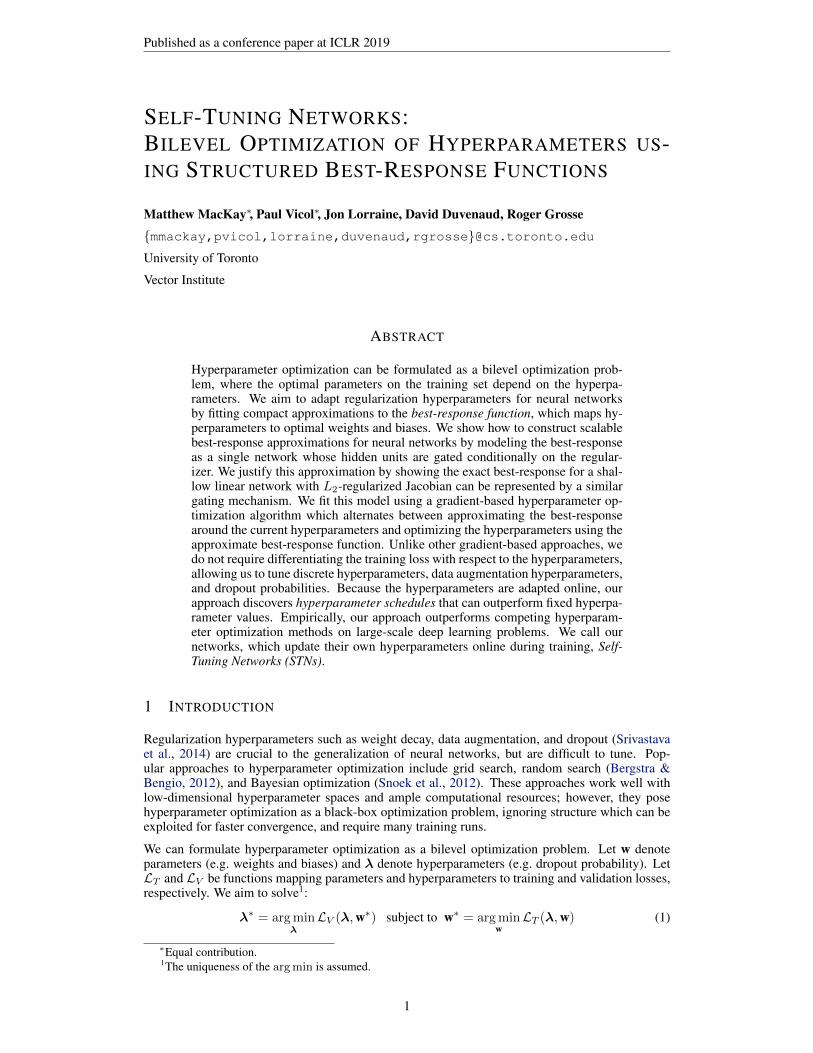
Given that the best-response function is a mapping from Rn to the high-dimensional weight spaceRm, why should we expect to be able to represent it compactly? And why in particular wouldequation 10 be a reasonable approximation? In this section, we exhibit a model whose best-responsefunction can be represented exactly using a minor variant of equation 10: a linear network withJacobian norm regularization. In particular, the best-response takes the form of a network whosehidden units are modulated conditionally on the hyperparameters.

Consider using a 2-layer linear network with weights w = (Q, s) ∈ RD×D × RD to predict targetst ∈ R from inputs x ∈ RD:

3We describe modifications for convolutional filters in Appendix C.4We illustrate how this is done for the PyTorch library (Paszke et al., 2017) in Appendix G.

4


Matmul

Change to principal component basis Project to 1-D Space

Matmul Add

Construct -dependent mask

Mask the hidden state

Matmul

Figure 1: Best-response architecture for an L2-Jacobian regularized two-layer linear network.

a(x;w) = Qx, y(x;w) = s>a(x;w) (12)

Suppose we use a squared-error loss regularized with an L2 penalty on the Jacobian ∂y/∂x, wherethe penalty weight λ lies in R and is mapped using exp to lie R+ :

LT (λ,w) =∑

(x,t)∈D

(y(x;w)− t)2 + 1

|D|exp(λ)

∥∥∥∥ ∂y∂x (x;w)

∥∥∥∥2 (13)

Theorem 2. Let w0 = (Q0, s0), where Q0 is the change-of-basis matrix to the principal compo-nents of the data matrix and s0 solves the unregularized version of Problem 13 givenQ0. Then thereexist v, c ∈ RD such that the best-response function5 w∗(λ) = (Q∗(λ), s∗(λ)) is:

Q∗(λ) = σ(λv + c)�row Q0, s∗(λ) = s0,

where σ is the sigmoid function.


Observe that y(x;w∗(λ)) can be implemented as a regular network with weights w0 = (Q0, s0)with an additional sigmoidal gating of its hidden units a(x;w∗(λ)):

a(x;w∗(λ)) = Q∗(λ)x = σ(λv + c)�row (Q0x) = σ(λv + c)�row a(x;w0) (14)

This architecture is shown in Figure 1. Inspired by this example, we use a similar gating of thehidden units to approximate the best-response for deep, nonlinear networks.

3.3 LINEAR BEST-RESPONSE APPROXIMATIONS

The sigmoidal gating architecture of the preceding section can be further simplified if one onlyneeds to approximate the best-response function for a small range of hyperparameter values. Inparticular, for a narrow enough hyperparameter distribution, a smooth best-response function can beapproximated by an affine function (i.e. its first-order Taylor approximation). Hence, we replace thesigmoidal gating with linear gating, in order that the weights be affine in the hyperparameters. Thefollowing theorem shows that, for quadratic lower-level objectives, using an affine approximationto the best-response function and minimizing Eε∼p(ε|σ) [f(λ+ ε, wφ(λ+ ε))] yields the correctbest-response Jacobian, thus ensuring gradient descent on the approximate objective F (λ, wφ(λ))converges to a local optimum:

Theorem 3. Suppose f is quadratic with ∂2f/∂w2 � 0, p(ε|σ) is Gaussian with mean 0 and varianceσ2I , and wφ is affine. Fix λ0 ∈ Rn and let φ∗ = argminφ Eε∼p(ε|σ) [f(λ+ ε, wφ(λ+ ε))]. Thenwe have wφ/∂λ(λ0) = ∂w∗

/∂λ(λ0).


5


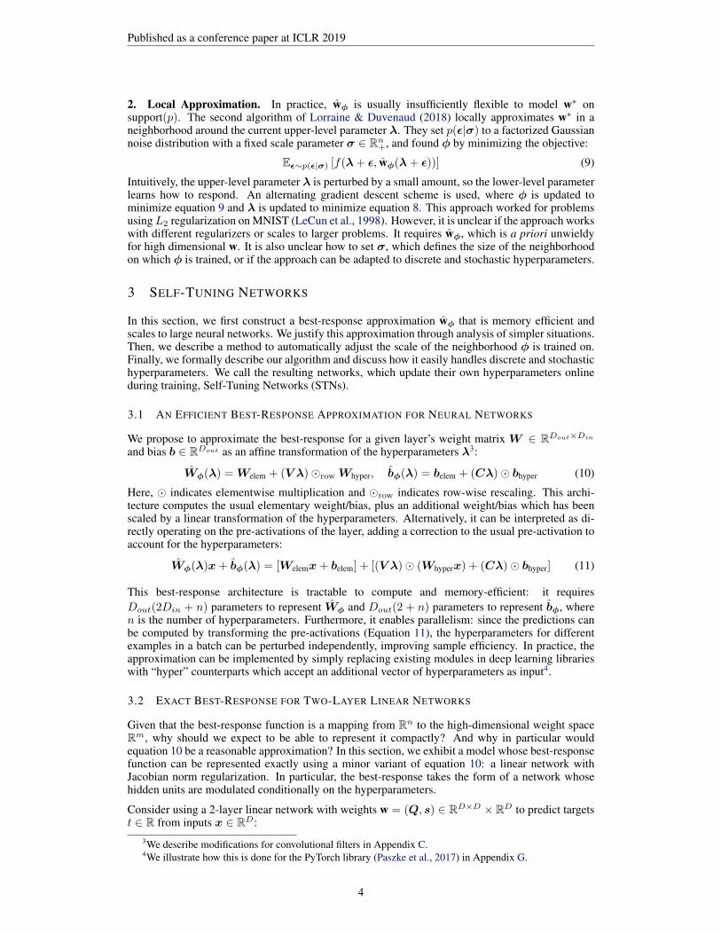
Legend: Exact best-response Approximate best-response Hyperparameter distribution

Figure 2: The effect of the sampled neighborhood. Left: If the sampled neighborhood is too small (e.g., apoint mass) the approximation learned will only match the exact best-response at the current hyperparameter,with no guarantee that its gradient matches that of the best-response. Middle: If the sampled neighborhood isnot too small or too wide, the gradient of the approximation will match that of the best-response. Right: If thesampled neighborhood is too wide, the approximation will be insufficiently flexible to model the best-response,and again the gradients will not match.

3.4 ADAPTING THE HYPERPARAMETER DISTRIBUTION

The entries of σ control the scale of the hyperparameter distribution on which φ is trained. Ifthe entries are too large, then wφ will not be flexible enough to capture the best-response over thesamples. However, the entries must remain large enough to force wφ to capture the shape locallyaround the current hyperparameter values. We illustrate this in Figure 2. As the smoothness of theloss landscape changes during training, it may be beneficial to vary σ.

To address these issues, we propose adjusting σ during training based on the sensitivity of the upper-level objective to the sampled hyperparameters. We include an entropy term weighted by τ ∈ R+

which acts to enlarge the entries of σ. The resulting objective is:

Eε∼p(ε|σ)[F (λ+ ε, wφ(λ+ ε))]− τH[p(ε|σ)] (15)

This is similar to a variational inference objective, where the first term is analogous to the negativelog-likelihood, but τ 6= 1. As τ ranges from 0 to 1, our objective interpolates between variationaloptimization (Staines & Barber, 2012) and variational inference, as noted by Khan et al. (2018).Similar objectives have been used in the variational inference literature for better training (Blundellet al., 2015) and representation learning (Higgins et al., 2017).

Minimizing the first term on its own eventually moves all probability mass towards an optimum λ∗,resulting in σ = 0 if λ∗ is an isolated local minimum. This compels σ to balance between shrinkingto decrease the first term while remaining sufficiently large to avoid a heavy entropy penalty. Whenbenchmarking our algorithm’s performance, we evaluate F (λ, wφ(λ)) at the deterministic currenthyperparameter λ0. (This is a common practice when using stochastic operations during training,such as batch normalization or dropout.)

3.5 TRAINING ALGORITHM

We now describe the complete STN training algorithm and discuss how it can tune hyperparametersthat other gradient-based algorithms cannot, such as discrete or stochastic hyperparameters. We usean unconstrained parametrization λ ∈ Rn of the hyperparameters. Let r denote the element-wisefunction which maps λ to the appropriate constrained space, which will involve a non-differentiablediscretization for discrete hyperparameters.

Let LT and LV denote training and validation losses which are (possibly stochastic, e.g., if usingdropout) functions of the hyperparameters and parameters. Define functions f, F by f(λ,w) =LT (r(λ),w) and F (λ,w) = LV (r(λ),w). STNs are trained by a gradient descent scheme whichalternates between updatingφ for Ttrain steps to minimize Eε∼p(ε|σ) [f(λ+ ε, wφ(λ+ ε))] (Eq. 9)and updating λ and σ for Tvalid steps to minimize Eε∼p(ε|σ)[F (λ+ ε, wφ(λ+ ε))]− τH[p(ε|σ)](Eq. 15). We give our complete algorithm as Algorithm 1 and show how it can be implemented incode in Appendix G. The possible non-differentiability of r due to discrete hyperparameters posesno problem. To estimate the derivative of Eε∼p(ε|σ) [f(λ+ ε, wφ(λ+ ε))] with respect to φ, wecan use the reparametrization trick and compute ∂f/∂w and ∂wφ/∂φ, neither of whose computationpaths involve the discretization r. To differentiate Eε∼p(ε|σ)[F (λ + ε, wφ(λ + ε))] − τH[p(ε|σ)]with respect to a discrete hyperparameter λi, there are two cases we must consider:

5This is an abuse of notation since there is not a unique solution to Problem 13 for each λ in general.

6


Algorithm 1 STN Training Algorithm

Initialize: Best-response approximation parameters φ, hy-perparameters λ, learning rates {αi}3i=1while not converged do

for t = 1, . . . , Ttrain doε ∼ p(ε|σ)φ← φ− α1

∂∂φf(λ+ ε, wφ(λ+ ε))

for t = 1, . . . , Tvalid doε ∼ p(ε|σ)λ← λ−α2

∂∂λ (F (λ+ ε, wφ(λ+ ε))− τH[p(ε|σ)])

σ ← σ−α3∂∂σ (F (λ+ ε, wφ(λ+ ε))− τH[p(ε|σ)])

Case 1: For most regularizationschemes, LV and hence F does notdepend on λi directly and thus theonly gradient is through wφ. Thus,the reparametrization gradient canbe used.

Case 2: If LV relies explic-itly on λi, then we can use theREINFORCE gradient estimator(Williams, 1992) to estimate thederivative of the expectation withrespect to λi. The number of hid-den units in a layer is an example ofa hyperparameter that requires this

approach since it directly affects the validation loss. We do not show this in Algorithm 1, since wedo not tune any hyperparameters which fall into this case.

4 EXPERIMENTS

We applied our method to convolutional networks and LSTMs (Hochreiter & Schmidhuber, 1997),yielding self-tuning CNNs (ST-CNNs) and self-tuning LSTMs (ST-LSTMs). We first investigatedthe behavior of STNs in a simple setting where we tuned a single hyperparameter, and found thatSTNs discovered hyperparameter schedules that outperformed fixed hyperparameter values. Next,we compared the performance of STNs to commonly-used hyperparameter optimization methodson the CIFAR-10 (Krizhevsky & Hinton, 2009) and PTB (Marcus et al., 1993) datasets.

4.1 HYPERPARAMETER SCHEDULES

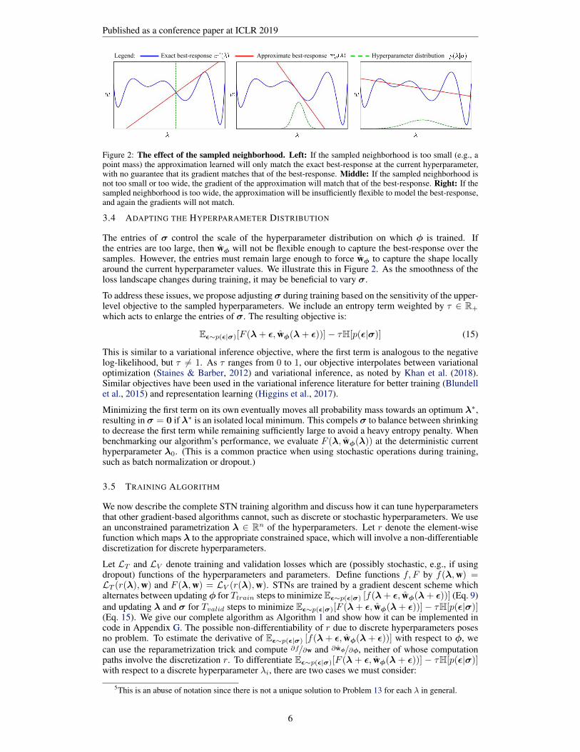
Due to the joint optimization of the hypernetwork weights and hyperparameters, STNs do not use asingle, fixed hyperparameter during training. Instead, STNs discover schedules for adapting the hy-perparameters online, which can outperform any fixed hyperparameter. We examined this behaviorin detail on the PTB corpus (Marcus et al., 1993) using an ST-LSTM to tune the output dropout rateapplied to the hidden units.

The schedule discovered by an ST-LSTM for output dropout, shown in Figure 3, outperforms thebest, fixed output dropout rate (0.68) found by a fine-grained grid search, achieving 82.58 vs 85.83validation perplexity. We claim that this is a consequence of the schedule, and not of regularizingeffects from sampling hyperparameters or the limited capacity of wφ.

To rule out the possibility that the improved performance is due to stochasticity introduced bysampling hyperparameters during STN training, we trained a standard LSTM while perturbing itsdropout rate around the best value found by grid search. We used (1) random Gaussian perturba-tions, and (2) sinusoid perturbations for a cyclic regularization schedule. STNs outperformed bothperturbation methods (Table 1), showing that the improvement is not merely due to hyperparameterstochasticity. Details and plots of each perturbation method are provided in Appendix F.

Method Val Test

p = 0.68, Fixed 85.83 83.19

p = 0.68 w/ Gaussian Noise 85.87 82.29

p = 0.68 w/ Sinusoid Noise 85.29 82.15

p = 0.78 (Final STN Value) 89.65 86.90

STN 82.58 79.02

LSTM w/ STN Schedule 82.87 79.93

Table 1: Comparing an LSTM trained with fixed and per-turbed output dropouts, an STN, and LSTM trained with theSTN schedule.

0 5k 10k 15k 20k 25kIteration

0.0

0.2

0.4

0.6

0.8

1.0

Outp

ut D

ropo

ut R

ate

Init=0.05Init=0.3Init=0.5Init=0.7Init=0.9

Figure 3: Dropout schedules found by the ST-LSTM for different initial dropout rates.

7


PTB CIFAR-10

Method Val Perplexity Test Perplexity Val Loss Test Loss

Grid Search 97.32 94.58 0.794 0.809

Random Search 84.81 81.46 0.921 0.752

Bayesian Optimization 72.13 69.29 0.636 0.651

STN 70.30 67.68 0.575 0.576

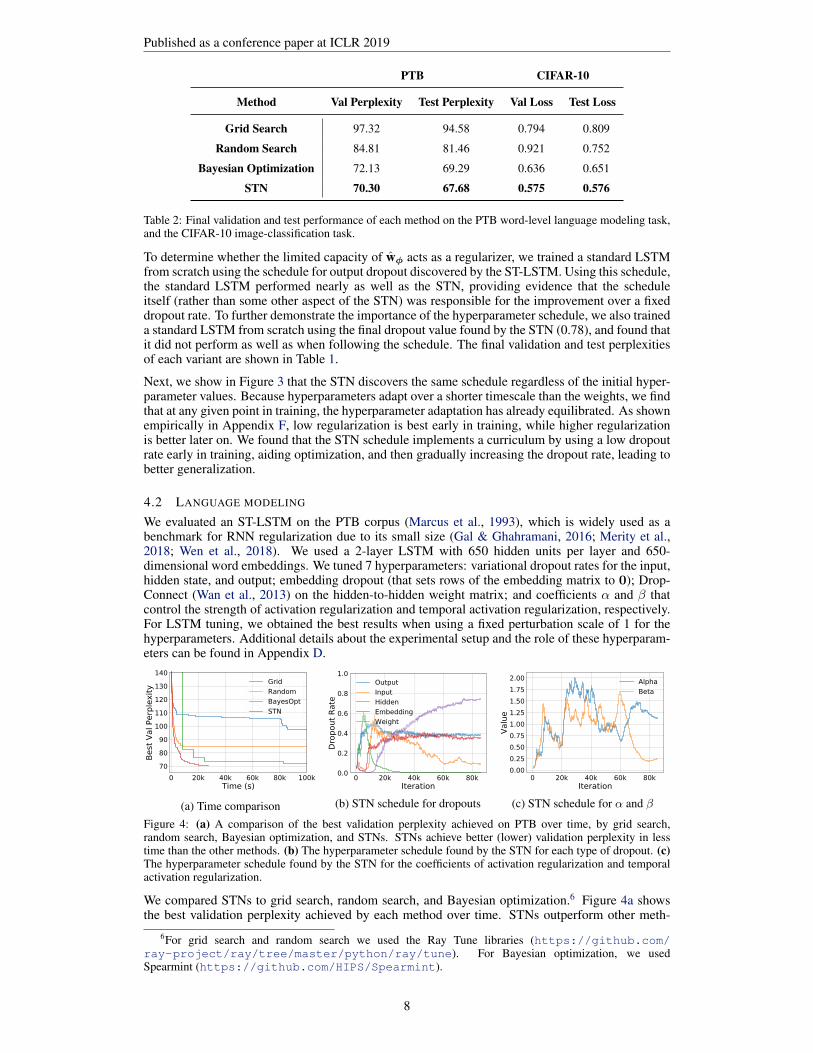
Table 2: Final validation and test performance of each method on the PTB word-level language modeling task,and the CIFAR-10 image-classification task.

To determine whether the limited capacity of wφ acts as a regularizer, we trained a standard LSTMfrom scratch using the schedule for output dropout discovered by the ST-LSTM. Using this schedule,the standard LSTM performed nearly as well as the STN, providing evidence that the scheduleitself (rather than some other aspect of the STN) was responsible for the improvement over a fixeddropout rate. To further demonstrate the importance of the hyperparameter schedule, we also traineda standard LSTM from scratch using the final dropout value found by the STN (0.78), and found thatit did not perform as well as when following the schedule. The final validation and test perplexitiesof each variant are shown in Table 1.

Next, we show in Figure 3 that the STN discovers the same schedule regardless of the initial hyper-parameter values. Because hyperparameters adapt over a shorter timescale than the weights, we findthat at any given point in training, the hyperparameter adaptation has already equilibrated. As shownempirically in Appendix F, low regularization is best early in training, while higher regularizationis better later on. We found that the STN schedule implements a curriculum by using a low dropoutrate early in training, aiding optimization, and then gradually increasing the dropout rate, leading tobetter generalization.

4.2 LANGUAGE MODELING

We evaluated an ST-LSTM on the PTB corpus (Marcus et al., 1993), which is widely used as abenchmark for RNN regularization due to its small size (Gal & Ghahramani, 2016; Merity et al.,2018; Wen et al., 2018). We used a 2-layer LSTM with 650 hidden units per layer and 650-dimensional word embeddings. We tuned 7 hyperparameters: variational dropout rates for the input,hidden state, and output; embedding dropout (that sets rows of the embedding matrix to 0); Drop-Connect (Wan et al., 2013) on the hidden-to-hidden weight matrix; and coefficients α and β thatcontrol the strength of activation regularization and temporal activation regularization, respectively.For LSTM tuning, we obtained the best results when using a fixed perturbation scale of 1 for thehyperparameters. Additional details about the experimental setup and the role of these hyperparam-eters can be found in Appendix D.

0 20k 40k 60k 80k 100kTime (s)

708090

100110120130140

Best

Val

Per

plex

ity

GridRandomBayesOptSTN

(a) Time comparison

0 20k 40k 60k 80kIteration

0.0

0.2

0.4

0.6

0.8

1.0

Drop

out R

ate

OutputInputHiddenEmbeddingWeight

(b) STN schedule for dropouts

0 20k 40k 60k 80kIteration

0.000.250.500.751.001.251.501.752.00

Valu

e

AlphaBeta

(c) STN schedule for α and β

Figure 4: (a) A comparison of the best validation perplexity achieved on PTB over time, by grid search,random search, Bayesian optimization, and STNs. STNs achieve better (lower) validation perplexity in lesstime than the other methods. (b) The hyperparameter schedule found by the STN for each type of dropout. (c)The hyperparameter schedule found by the STN for the coefficients of activation regularization and temporalactivation regularization.

We compared STNs to grid search, random search, and Bayesian optimization.6 Figure 4a showsthe best validation perplexity achieved by each method over time. STNs outperform other meth-

6For grid search and random search we used the Ray Tune libraries (https://github.com/ray-project/ray/tree/master/python/ray/tune). For Bayesian optimization, we usedSpearmint (https://github.com/HIPS/Spearmint).

8

https://github.com/ray-project/ray/tree/master/python/ray/tune

https://github.com/ray-project/ray/tree/master/python/ray/tune

https://github.com/HIPS/Spearmint


0 40k 80k 120kIteration

0.0

0.2

0.4

0.6

0.8

1.0

Drop

out R

ate

Layer 0Layer 1Layer 2Layer 3Layer 4InputFC 0FC 1


0.0

0.1

0.2

0.3

0.4

0.5

Amou

nt o

f Noi

se

HueContrastSaturationBrightnessInscale


0

2

4

6

Num

ber/L

engt

h of

Hol

es Cutout holesCutout length

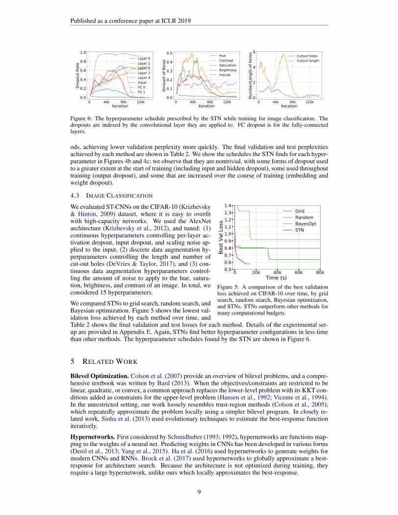
Figure 6: The hyperparameter schedule prescribed by the STN while training for image classification. Thedropouts are indexed by the convolutional layer they are applied to. FC dropout is for the fully-connectedlayers.

ods, achieving lower validation perplexity more quickly. The final validation and test perplexitiesachieved by each method are shown in Table 2. We show the schedules the STN finds for each hyper-parameter in Figures 4b and 4c; we observe that they are nontrivial, with some forms of dropout usedto a greater extent at the start of training (including input and hidden dropout), some used throughouttraining (output dropout), and some that are increased over the course of training (embedding andweight dropout).

4.3 IMAGE CLASSIFICATION

0 20k 40k 60k 80kTime (s)

0.50.60.70.80.91.01.11.21.31.4

Best

Val

Los

sGridRandomBayesOptSTN

Figure 5: A comparison of the best validationloss achieved on CIFAR-10 over time, by gridsearch, random search, Bayesian optimization,and STNs. STNs outperform other methods formany computational budgets.

We evaluated ST-CNNs on the CIFAR-10 (Krizhevsky& Hinton, 2009) dataset, where it is easy to overfitwith high-capacity networks. We used the AlexNetarchitecture (Krizhevsky et al., 2012), and tuned: (1)continuous hyperparameters controlling per-layer ac-tivation dropout, input dropout, and scaling noise ap-plied to the input, (2) discrete data augmentation hy-perparameters controlling the length and number ofcut-out holes (DeVries & Taylor, 2017), and (3) con-tinuous data augmentation hyperparameters control-ling the amount of noise to apply to the hue, satura-tion, brightness, and contrast of an image. In total, weconsidered 15 hyperparameters.

We compared STNs to grid search, random search, andBayesian optimization. Figure 5 shows the lowest val-idation loss achieved by each method over time, andTable 2 shows the final validation and test losses for each method. Details of the experimental set-up are provided in Appendix E. Again, STNs find better hyperparameter configurations in less timethan other methods. The hyperparameter schedules found by the STN are shown in Figure 6.

5 RELATED WORK

Bilevel Optimization. Colson et al. (2007) provide an overview of bilevel problems, and a compre-hensive textbook was written by Bard (2013). When the objectives/constraints are restricted to belinear, quadratic, or convex, a common approach replaces the lower-level problem with its KKT con-ditions added as constraints for the upper-level problem (Hansen et al., 1992; Vicente et al., 1994).In the unrestricted setting, our work loosely resembles trust-region methods (Colson et al., 2005),which repeatedly approximate the problem locally using a simpler bilevel program. In closely re-lated work, Sinha et al. (2013) used evolutionary techniques to estimate the best-response functioniteratively.

Hypernetworks. First considered by Schmidhuber (1993; 1992), hypernetworks are functions map-ping to the weights of a neural net. Predicting weights in CNNs has been developed in various forms(Denil et al., 2013; Yang et al., 2015). Ha et al. (2016) used hypernetworks to generate weights formodern CNNs and RNNs. Brock et al. (2017) used hypernetworks to globally approximate a best-response for architecture search. Because the architecture is not optimized during training, theyrequire a large hypernetwork, unlike ours which locally approximates the best-response.

9


Gradient-Based Hyperparameter Optimization. There are two main approaches. The first ap-proach approximates w∗(λ0) using wT (λ0,w0), the value of w after T steps of gradient descent onf with respect to w starting at (λ0,w0). The descent steps are differentiated through to approxi-mate ∂w∗

/∂λ(λ0) ≈ ∂wT/∂λ(λ0,w0). This approach was proposed by Domke (2012) and used byMaclaurin et al. (2015), Luketina et al. (2016) and Franceschi et al. (2018). The second approachuses the Implicit Function Theorem to derive ∂w∗

/∂λ(λ0) under certain conditions. This was firstdeveloped for hyperparameter optimization in neural networks (Larsen et al., 1996) and developedfurther by Pedregosa (2016). Similar approaches have been used for hyperparameter optimizationin log-linear models (Foo et al., 2008), kernel selection (Chapelle et al., 2002; Seeger, 2007), andimage reconstruction (Kunisch & Pock, 2013; Calatroni et al., 2015). Both approaches strugglewith certain hyperparameters, since they differentiate gradient descent or the training loss with re-spect to the hyperparameters. In addition, differentiating gradient descent becomes prohibitivelyexpensive as the number of descent steps increases, while implicitly deriving ∂w∗

/∂λ requires usingHessian-vector products with conjugate gradient solvers to avoid directly computing the Hessian.

Model-Based Hyperparameter Optimization. A common model-based approach is Bayesian op-timization, which models p(r|λ,D), the conditional probability of the performance on some metricr given hyperparameters λ and a dataset D = {(λi, ri)}. We can model p(r|λ,D) with variousmethods (Hutter et al., 2011; Bergstra et al., 2011; Snoek et al., 2012; 2015). D is constructed itera-tively, where the next λ to train on is chosen by maximizing an acquisition functionC(λ; p(r|λ,D))which balances exploration and exploitation. Training each model to completion can be avoided ifassumptions are made on learning curve behavior (Swersky et al., 2014; Klein et al., 2017). Theseapproaches require building inductive biases into p(r|λ,D) which may not hold in practice, do nottake advantage of the network structure when used for hyperparameter optimization, and do not scalewell with the number of hyperparameters. However, these approaches have consistency guaranteesin the limit, unlike ours.

Model-Free Hyperparameter Optimization. Model-free approaches include grid search and ran-dom search. Bergstra & Bengio (2012) advocated using random search over grid search. SuccessiveHalving (Jamieson & Talwalkar, 2016) and Hyperband (Li et al., 2017) extend random search byadaptively allocating resources to promising configurations using multi-armed bandit techniques.These methods ignore structure in the problem, unlike ours which uses rich gradient information.However, it is trivial to parallelize model-free methods over computing resources and they tend toperform well in practice.

Hyperparameter Scheduling. Population Based Training (PBT) (Jaderberg et al., 2017) considersschedules for hyperparameters. In PBT, a population of networks is trained in parallel. The per-formance of each network is evaluated periodically, and the weights of under-performing networksare replaced by the weights of better-performing ones; the hyperparameters of the better networkare also copied and randomly perturbed for training the new network clone. In this way, a singlemodel can experience different hyperparameter settings over the course of training, implementinga schedule. STNs replace the population of networks by a single best-response approximation anduse gradients to tune hyperparameters during a single training run.

6 CONCLUSION

We introduced Self-Tuning Networks (STNs), which efficiently approximate the best-response ofparameters to hyperparameters by scaling and shifting their hidden units. This allowed us to usegradient-based optimization to tune various regularization hyperparameters, including discrete hy-perparameters. We showed that STNs discover hyperparameter schedules that can outperform fixedhyperparameters. We validated the approach on large-scale problems and showed that STNs achievebetter generalization performance than competing approaches, in less time. We believe STNs offera compelling path towards large-scale, automated hyperparameter tuning for neural networks.

ACKNOWLEDGMENTS

We thank Matt Johnson for helpful discussions and advice. MM is supported by an NSERC CGS-M award, and PV is supported by an NSERC PGS-D award. RG acknowledges support from theCIFAR Canadian AI Chairs program.

10


REFERENCES

Eugene L Allgower and Kurt Georg. Numerical Continuation Methods: An Introduction, volume 13.Springer Science & Business Media, 2012.

Jonathan F Bard. Practical Bilevel Optimization: Algorithms and Applications, volume 30. SpringerScience & Business Media, 2013.

Yoshua Bengio, Jerome Louradour, Ronan Collobert, and Jason Weston. Curriculum learning. InInternational Conference on Machine Learning, pp. 41–48. ACM, 2009.

James Bergstra and Yoshua Bengio. Random search for hyper-parameter optimization. Journal ofMachine Learning Research, 13:281–305, 2012.

James S. Bergstra, Remi Bardenet, Yoshua Bengio, and Balazs Kegl. Algorithms for hyper-parameter optimization. In Advances in Neural Information Processing Systems, pp. 2546–2554.2011.

Charles Blundell, Julien Cornebise, Koray Kavukcuoglu, and Daan Wierstra. Weight uncertainty inneural networks. arXiv preprint arXiv:1505.05424, 2015.

Andrew Brock, Theodore Lim, James M Ritchie, and Nick Weston. SMASH: One-shot modelarchitecture search through hypernetworks. arXiv preprint arXiv:1708.05344, 2017.

Luca Calatroni, Cao Chung, Juan Carlos De Los Reyes, Carola-Bibiane Schonlieb, and TuomoValkonen. Bilevel approaches for learning of variational imaging models. arXiv preprintarXiv:1505.02120, 2015.

Olivier Chapelle, Vladimir Vapnik, Olivier Bousquet, and Sayan Mukherjee. Choosing multipleparameters for Support Vector Machines. Machine Learning, 46(1-3):131–159, 2002.

Benoıt Colson, Patrice Marcotte, and Gilles Savard. A trust-region method for nonlinear bilevelprogramming: Algorithm and computational experience. Computational Optimization and Ap-plications, 30(3):211–227, 2005.

Benoıt Colson, Patrice Marcotte, and Gilles Savard. An overview of bilevel optimization. Annals ofOperations Research, 153(1):235–256, 2007.

Misha Denil, Babak Shakibi, Laurent Dinh, Nando De Freitas, et al. Predicting parameters in deeplearning. In Advances in Neural Information Processing Systems, pp. 2148–2156, 2013.

Terrance DeVries and Graham W Taylor. Improved regularization of convolutional neural networkswith cutout. arXiv preprint arXiv:1708.04552, 2017.

Justin Domke. Generic methods for optimization-based modeling. In Proceedings of MachineLearning Research, pp. 318–326, 2012.

John Duchi. Properties of the trace and matrix derivatives, 2007. URL https://web.stanford.edu/˜jduchi/projects/matrix_prop.pdf.

Anthony V Fiacco and Yo Ishizuka. Sensitivity and stability analysis for nonlinear programming.Annals of Operations Research, 27(1):215–235, 1990.

Chuan-sheng Foo, Chuong B Do, and Andrew Y Ng. Efficient multiple hyperparameter learning forlog-linear models. In Advances in Neural Information Processing Systems, pp. 377–384, 2008.

Luca Franceschi, Paolo Frasconi, Saverio Salzo, and Massimilano Pontil. Bilevel programming forhyperparameter optimization and meta-learning. arXiv preprint arXiv:1806.04910, 2018.

Yarin Gal and Zoubin Ghahramani. A theoretically grounded application of dropout in recurrentneural networks. In Advances in Neural Information Processing Systems, pp. 1027–1035, 2016.

Robert Gibbons. A Primer in Game Theory. Harvester Wheatsheaf, 1992.

11

https://web.stanford.edu/~jduchi/projects/matrix_prop.pdf

https://web.stanford.edu/~jduchi/projects/matrix_prop.pdf


Ian Goodfellow, Jean Pouget-Abadie, Mehdi Mirza, Bing Xu, David Warde-Farley, Sherjil Ozair,Aaron Courville, and Yoshua Bengio. Generative adversarial nets. In Advances in Neural Infor-mation Processing Systems, pp. 2672–2680, 2014.

David Ha, Andrew Dai, and Quoc V Le. Hypernetworks. arXiv preprint arXiv:1609.09106, 2016.

Pierre Hansen, Brigitte Jaumard, and Gilles Savard. New branch-and-bound rules for linear bilevelprogramming. SIAM Journal on Scientific and Statistical Computing, 13(5):1194–1217, 1992.

Trevor Hastie, Robert Tibshirani, and Jerome Friedman. The Elements of Statistical Learning.Springer Series in Statistics. Springer, New York, NY, USA, 2001.

Irina Higgins, Loic Matthey, Arka Pal, Christopher Burgess, Xavier Glorot, Matthew Botvinick,Shakir Mohamed, and Alexander Lerchner. Beta-VAE: Learning basic visual concepts with aconstrained variational framework. In International Conference on Learning Representations,2017.

Sepp Hochreiter and Jurgen Schmidhuber. Long short-term memory. Neural Computation, 9(8):1735–1780, 1997.

Frank Hutter, Holger H Hoos, and Kevin Leyton-Brown. Sequential model-based optimizationfor general algorithm configuration. In International Conference on Learning and IntelligentOptimization, pp. 507–523. Springer, 2011.

Max Jaderberg, Valentin Dalibard, Simon Osindero, Wojciech M Czarnecki, Jeff Donahue, AliRazavi, Oriol Vinyals, Tim Green, Iain Dunning, Karen Simonyan, et al. Population-based train-ing of neural networks. arXiv preprint arXiv:1711.09846, 2017.

Kevin Jamieson and Ameet Talwalkar. Non-stochastic best arm identification and hyperparameteroptimization. In International Conference on Artificial Intelligence and Statistics, 2016.

Mohammad Emtiyaz Khan, Didrik Nielsen, Voot Tangkaratt, Wu Lin, Yarin Gal, and Akash Srivas-tava. Fast and scalable Bayesian deep learning by weight-perturbation in Adam. arXiv preprintarXiv:1806.04854, 2018.

Aaron Klein, Stefan Falkner, Jost Tobias Springenberg, and Frank Hutter. Learning curve predictionwith Bayesian neural networks. In International Conference on Learning Representations, 2017.

Alex Krizhevsky and Geoffrey Hinton. Learning multiple layers of features from tiny images. InTechnical Report, University of Toronto, 2009.

Alex Krizhevsky, Ilya Sutskever, and Geoffrey E Hinton. ImageNet classification with deep convo-lutional neural networks. In Advances in Neural Information Processing Systems, pp. 1097–1105,2012.

Karl Kunisch and Thomas Pock. A bilevel optimization approach for parameter learning in varia-tional models. SIAM Journal on Imaging Sciences, 6(2):938–983, 2013.

Jan Larsen, Lars Kai Hansen, Claus Svarer, and M Ohlsson. Design and regularization of neuralnetworks: The optimal use of a validation set. In IEEE Workshop on Neural Networks for SignalProcessing, pp. 62–71. IEEE, 1996.

Yann LeCun, Leon Bottou, Yoshua Bengio, and Patrick Haffner. Gradient-based learning applied todocument recognition. Proceedings of the IEEE, 86(11):2278–2324, 1998.

Lisha Li, Kevin Jamieson, Giulia DeSalvo, Afshin Rostamizadeh, and Ameet Talwalkar. Hyper-band: Bandit-based configuration evaluation for hyperparameter optimization. Journal of Ma-chine Learning Research, 18(1):6765–6816, 2017.

Jonathan Lorraine and David Duvenaud. Stochastic hyperparameter optimization through hypernet-works. arXiv preprint arXiv:1802.09419, 2018.

Jelena Luketina, Mathias Berglund, Klaus Greff, and Tapani Raiko. Scalable gradient-based tuningof continuous regularization hyperparameters. In International Conference on Machine Learning,pp. 2952–2960, 2016.

12


Dougal Maclaurin, David Duvenaud, and Ryan Adams. Gradient-based hyperparameter optimiza-tion through reversible learning. In International Conference on Machine Learning, pp. 2113–2122, 2015.

Mitchell P Marcus, Mary Ann Marcinkiewicz, and Beatrice Santorini. Building a large annotatedcorpus of English: The Penn Treebank. Computational Linguistics, 19(2):313–330, 1993.

Stephen Merity, Nitish Shirish Keskar, and Richard Socher. Regularizing and optimizing LSTMlanguage models. International Conference on Learning Representations, 2018.

Lars Mescheder, Sebastian Nowozin, and Andreas Geiger. The numerics of GANs. In Advances inNeural Information Processing Systems, pp. 1825–1835, 2017.

Luke Metz, Ben Poole, David Pfau, and Jascha Sohl-Dickstein. Unrolled generative adversarialnetworks. arXiv preprint arXiv:1611.02163, 2016.

Yurii Nesterov. Introductory Lectures on Convex Optimization: A Basic Course, volume 87.Springer Science & Business Media, 2013.

Adam Paszke, Sam Gross, Soumith Chintala, Gregory Chanan, Edward Yang, Zachary DeVito,Zeming Lin, Alban Desmaison, Luca Antiga, and Adam Lerer. Automatic differentiation inPyTorch. In Advances in Neural Information Processing Workshop, 2017.

Fabian Pedregosa. Hyperparameter optimization with approximate gradient. In International Con-ference on Machine Learning, pp. 737–746, 2016.

Jurgen Schmidhuber. Learning to control fast-weight memories: An alternative to dynamic recurrentnetworks. Neural Computation, 4(1):131–139, 1992.

Jurgen Schmidhuber. A ‘self-referential’ weight matrix. In International Conference on ArtificialNeural Networks, pp. 446–450. Springer, 1993.

Matthias Seeger. Cross-validation optimization for large scale hierarchical classification kernelmethods. In Advances in Neural Information Processing Systems, pp. 1233–1240, 2007.

Ankur Sinha, Pekka Malo, and Kalyanmoy Deb. Efficient evolutionary algorithm for single-objective bilevel optimization. arXiv preprint arXiv:1303.3901, 2013.

Jasper Snoek, Hugo Larochelle, and Ryan P Adams. Practical Bayesian optimization of machinelearning algorithms. In Advances in Neural Information Processing Systems, pp. 2951–2959,2012.

Jasper Snoek, Oren Rippel, Kevin Swersky, Ryan Kiros, Nadathur Satish, Narayanan Sundaram,Mostofa Patwary, M Prabhat, and Ryan Adams. Scalable Bayesian optimization using deep neuralnetworks. In International Conference on Machine Learning, pp. 2171–2180, 2015.

Nitish Srivastava, Geoffrey Hinton, Alex Krizhevsky, Ilya Sutskever, and Ruslan Salakhutdinov.Dropout: A simple way to prevent neural networks from overfitting. The Journal of MachineLearning Research, 15(1):1929–1958, 2014.

Joe Staines and David Barber. Variational optimization. arXiv preprint arXiv:1212.4507, 2012.

Kevin Swersky, Jasper Snoek, and Ryan Prescott Adams. Freeze-thaw Bayesian optimization. arXivpreprint arXiv:1406.3896, 2014.

Luis Vicente, Gilles Savard, and Joaquim Judice. Descent approaches for quadratic bilevel program-ming. Journal of Optimization Theory and Applications, 81(2):379–399, 1994.

Heinrich Von Stackelberg. Market Structure and Equilibrium. Springer Science & Business Media,2010.

Li Wan, Matthew Zeiler, Sixin Zhang, Yann Le Cun, and Rob Fergus. Regularization of neuralnetworks using Dropconnect. In International Conference on Machine Learning, pp. 1058–1066,2013.

13


Yeming Wen, Paul Vicol, Jimmy Ba, Dustin Tran, and Roger Grosse. Flipout: Efficient pseudo-independent weight perturbations on mini-batches. International Conference on Learning Repre-sentations, 2018.

Ronald J Williams. Simple statistical gradient-following algorithms for connectionist reinforcementlearning. Machine Learning, 8(3-4):229–256, 1992.

Zichao Yang, Marcin Moczulski, Misha Denil, Nando de Freitas, Alex Smola, Le Song, and ZiyuWang. Deep fried convnets. In International Conference on Computer Vision, pp. 1476–1483,2015.

Wojciech Zaremba, Ilya Sutskever, and Oriol Vinyals. Recurrent neural network regularization.arXiv preprint arXiv:1409.2329, 2014.

Barret Zoph and Quoc V Le. Neural architecture search with reinforcement learning. arXiv preprintarXiv:1611.01578, 2016.

14


A TABLE OF NOTATION

Table 3: Table of Notation

λ,w Hyperparameters and parameters

λ0,w0 Current, fixed hyperparameters and parameters

n,m Hyperparameter and elementary parameter dimension

f(λ,w), F (λ,w) Lower-level & upper-level objective

r Function mapping unconstrained hyperparameters to the appropriate restricted space

LT (λ,w),LV (λ,w) Training loss & validation loss - (LT (r(λ),w),LV (r(λ),w)) = (f(λ,w), F (λ,w))

w∗(λ) Best-response of the parameters to the hyperparameters

F ∗(λ) Single-level objective from best-response, equals F (λ,w∗(λ))

λ∗ Optimal hyperparameters

wφ(λ) Parametric approximation to the best-response function

φ Approximate best-response parameters

σ Scale of the hyperparameter noise distribution

σ The sigmoid function

ε Sampled perturbation noise, to be added to hyperparameters

p(ε|σ), p(λ|σ) The noise distribution and induced hyperparameter distribution

α A learning rate

Ttrain, Tvalid Number of training steps on the training and validation data

x, t An input datapoint and its associated target

D A data set consisting of tuples of inputs and targets

D The dimensionality of input data

y(x,w) Prediction function for input data x and elementary parameters w

�row Row-wise rescaling - not elementwise multiplication

Q, s First and second layer weights of the linear network in Problem 13

Q0, s0 The basis change matrix and solution to the unregularized Problem 13

Q∗(λ), s∗(λ) The best response weights of the linear network in Problem 13

a(x;w) Activations of hidden units in the linear network of Problem 13

W , b A layer’s weight matrix and bias

Dout, Din A layer’s input dimensionality and output dimensionality∂LT (λ,w)

∂λ The (validation loss) direct (hyperparameter) gradient∂w∗(λ)∂λ The (elementary parameter) response gradient

∂LT (λ,w∗(λ))∂w∗(λ)

∂w∗(λ)∂λ The (validation loss) response gradient

dLT (λ,w)dλ The hyperparameter gradient: a sum of the validation losses direct and response gradients

15


B PROOFS

B.1 LEMMA 1

Because w0 solves Problem 4b given λ0, by the first-order optimality condition we must have:

∂f

∂w(λ0,w0) = 0 (16)

The Jacobian of ∂f/∂w decomposes as a block matrix with sub-blocks given by:[∂2f∂λ∂w

∂2f∂w2

](17)

We know that f is C2 in some neighborhood of (λ0,w0), so ∂f/∂w is continuously differentiablein this neighborhood. By assumption, the Hessian ∂2f/∂w2 is positive definite and hence invertibleat (λ0,w0). By the Implicit Function Theorem, there exists a neighborhood V of λ0 and a uniquecontinuously differentiable function w∗ : V → Rm such that ∂f/∂w(λ,w∗(λ)) = 0 for λ ∈ V andw∗(λ0) = w0.

Furthermore, by continuity we know that there is a neighborhood W1 ×W2 of (λ0,w0) such that∂2f/∂w2 is positive definite on this neighborhood. Setting U = V ∩ W1 ∩ (w∗)−1(W2), we canconclude that ∂2f/∂w2(λ,w∗(λ)) � 0 for all λ ∈ U . Combining this with ∂f/∂w(λ,w∗(λ)) = 0 andusing second-order sufficient optimality conditions, we conclude that w∗(λ) is the unique solutionto Problem 4b for all λ ∈ U .

B.2 LEMMA 2

This discussion mostly follows from Hastie et al. (2001). We letX ∈ RN×D denote the data matrixwhere N is the number of training examples and D is the dimensionality of the data. We let t ∈ RNdenote the associated targets. We can write the SVD decomposition ofX as:

X = UDV > (18)

where U and V are N × D and D × D orthogonal matrices and D is a diagonal matrix withentries d1 ≥ d2 ≥ · · · ≥ dD > 0. We next simplify the function y(x;w) by setting u = s>Q, sothat y(x;w) = s>Qx = u>x. We see that the Jacobian ∂y/∂x ≡ u is constant, and Problem 13simplifies to standardL2-regularized least-squares linear regression with the following loss function:∑

(x,t)∈D

(u>x− t)2 + 1

|D|exp(λ) ‖u‖2 (19)

It is well-known (see Hastie et al. (2001), Chapter 3) that the optimal solution u∗(λ) minimizingEquation 19 is given by:

u∗(λ) = (X>X + exp(λ)I)−1X>t = V (D2 + exp(λ)I)−1DU>t (20)

Furthermore, the optimal solution u∗ to the unregularized version of Problem 19 is given by:

u∗ = V D−1U>t (21)

Recall that we defined Q0 = V >, i.e., the change-of-basis matrix from the standard basis to theprincipal components of the data matrix, and we defined s0 to solve the unregularized regressionproblem givenQ0. Thus, we require thatQ>0 s0 = u∗ which implies s0 =D−1U>t.

There are not unique solutions to Problem 13, so we take any functions Q(λ), s(λ) which sat-isfy Q(λ)>s(λ) = v∗(λ) as “best-response functions”. We will show that our chosen functionsQ∗(λ) = σ(λv+ c)�rowQ0 and s∗(λ) = s0, where v = −1 and ci = 2 log(di) for i = 1, . . . , D,meet this criteria. We start by noticing that for any d ∈ R+, we have:

σ(−λ+ 2 log(d)) =1

1 + exp(λ− 2 log(d))=

1

1 + d−2 exp(λ)=

d2

d2 + exp(λ)(22)

16


It follows that:

Q∗(λ)>s∗(λ) = [σ(λv + c)�row Q0]>s0 (23)

=

diagσ(−λ+ 2 log(d1))

...

σ(−λ+ 2 log(dD))

Q0

>

s0 (24)

= Q>0

diag

d21d21+exp(λ)

...d2D

d2D+exp(λ)

s0 (25)

= V

diag

d21d21+exp(λ)

...d2D

d2D+exp(λ)

D−1U>t (26)

= V

diag

d1d21+exp(λ)

...dD

d2D+exp(λ)

U>t (27)

= V[(D2 + exp(λ)I)−1D

]U>t (28)

= v∗(λ) (29)

B.3 THEOREM 3

By assumption f is quadratic, so there existA ∈ Rn×n,B ∈ Rn×m,C ∈ Rm×m and d ∈ Rn, e ∈Rm such that:

f(λ,w) =1

2

(λ> w>

)( A B

B> C

)(λ

w

)+ d>λ+ e>w (30)

One can easily compute that:∂f

∂w(λ,w) = B>λ+Cw + e (31)

∂2f

∂w2(λ,w) = C (32)

Since we assume ∂2f/∂w2 � 0, we must have C � 0. Setting the derivative equal to 0 and usingsecond-order sufficient conditions, we have:

w∗(λ) = −C−1(e+B>λ) (33)

Hence, we find:∂w∗

∂λ(λ) = −C−1B> (34)

We let wφ(λ) = Uλ+ b, and define f to be the function given by:

f(λ,U , b,σ) = Eε∼p(ε|σ) [f(λ+ ε,U(λ+ ε) + b)] (35)

Substituting and simplifying:

f(λ0,U , b, σ) = Eε∼p(ε|σ)[1

2(λ0 + ε)

>A(λ0 + ε) + (λ0 + ε)>B(U(λ0 + ε) + b)

+1

2(U(λ0 + ε) + b)

>C(U(λ0 + ε) + b)

+ d>(λ0 + ε) + e>(U(λ0 + ε) + b)

](36)

17


Expanding, we find that equation 36 is equal to:

Eε∼p(ε|σ)[

1 + 2 + 3 + 4]

(37)

where we have:1 =

1

2

(λ>0 Aλ0 + 2ε>Aλ0 + ε

>Aε)

(38)

2 = λ>0 BUλ0 + λ>0 BUε+ λ

>0 Bb+ ε

>BUλ0 + ε>BUε+ ε>Bb (39)

3 =1

2(λ>0 U

>CUλ0 + λ0U>CUε+ λ0U

>Cb+ ε>U>CUλ0

+ ε>U>CUε+ ε>U>Cb+ b>CUλ0 + b>CUε+ b>Cb) (40)

4 = d>λ0 + d>ε+ e>Uλ0 + e

>Uε+ e>b (41)We can simplify these expressions considerably by using linearity of expectation and that ε ∼ p(ε|σ)has mean 0:

Eε∼p(ε|σ)[

1]=

1

2λ>0 Aλ0 (42)

Eε∼p(ε|σ)[

2]= λ>0 BUλ0 + λ

>0 Bb+ Eε∼p(ε|σ)

[ε>BUε

](43)

Eε∼p(ε|σ)[

3]=

1

2(λ>0 U

>CUλ0 + λ0U>Cb+

Eε∼p(ε|σ)[ε>U>CUε

]+ b>CUλ0 + b

>Cb) (44)

Eε∼p(ε|σ)[

4]= d>λ0 + e

>Uλ0 + e>b (45)

We can use the cyclic property of the Trace operator, Eε∼p(ε|σ)[εε>] = σ2I , and commutability of

expectation and a linear operator to simplify the expectations of 2 and 3 :

Eε∼p(ε|σ)[

2]= λ>0 BUλ0 + λ

>0 Bb+Tr

[σ2BU

](46)

Eε∼p(ε|σ)[

3]=

1

2(λ>0 U

>CUλ0 + λ0U>Cb+

Tr[σ2U>CU

]+ b>CUλ0 + b

>Cb) (47)

We can then differentiate f by making use of various matrix-derivative equalities (Duchi, 2007) tofind:

∂f

∂b(λ0,U , b, σ) =

1

2C>Uλ0 +

1

2CUλ0 +B

>λ0 + e+Cb (48)

∂f

∂U(λ0,U , b, σ) = B

>λ0λ>0 + σ2B> +Cbλ>0 + eλ>0 +CUλ0λ

>0 + σ2CU (49)

Setting the derivative ∂f/∂b(λ0,U , b, σ) equal to 0, we have:

b = −C−1(C>Uλ0 +B>λ0 + e) (50)

Setting the derivative for ∂f/∂U(λ0,U , b, σ) equal to 0, we have:

CU(λ0λ>0 + σ2C) = −B>λ0λ

>0 − σ2B> −Cbλ>0 − eλ>0 (51)

Substituting the expression for b given by equation 50 into equation 51 and simplifying gives:

CU(λ0λ>0 + σ2I) = −σ2B> +CUλ0λ

>0 (52)

=⇒ σ2CU = −σ2B> (53)

=⇒ U = −C−1B> (54)This is exactly the best-response Jacobian ∂w∗

/∂λ(λ) as given by Equation 34. Substituting U =C−1B into the equation 50 gives:

b = C−1B>λ0 −C−1B>λ0 −C−1e (55)This is w∗(λ0) − ∂w∗

/∂λ(λ0), thus the approximate best-response is exactly the first-order Taylorseries of w∗ about λ0.

18


B.4 BEST-RESPONSE GRADIENT LEMMA

Lemma 4. Under the same conditions as Lemma 1 and using the same notation, for all λ ∈ U , wehave that:

∂w∗

∂λ(λ) = −

[∂2f

∂w2(λ,w∗(λ))

]−1∂2f

∂λ∂w(λ,w∗(λ)) (56)

Proof. Define ι∗ : U → Rn×Rm by ι∗(λ) = (λ,w∗(λ)). By first-order optimality conditions, weknow that: (

∂f

∂w◦ ι∗)(λ) = 0 ∀λ ∈ U (57)

Hence, for all λ ∈ U :

0 =∂

∂λ

(∂f

∂w◦ ι∗)(λ) (58)

=∂2f

∂w2(ι∗(λ))

∂w∗

∂λ(λ) +

∂2f

∂λ∂w(ι∗(λ)) (59)

=∂2f

∂w2(λ,w∗(λ))

∂w∗

∂λ(λ) +

∂2f

∂λ∂w(λ,w∗(λ)) (60)

Rearranging gives Equation 56.

C BEST-RESPONSE APPROXIMATIONS FOR CONVOLUTIONAL FILTERS

We let L denote the number of layers, Cl the number of channels in layer l’s feature map, and Kl

the size of the kernel in layer l. We let W l,c ∈ RCl−1×Kl×Kl and bl,c ∈ R denote the weight andbias respectively of the cth convolution kernel in layer l (so c ∈ {1, . . . , Cl}). For ul,c,al,c ∈ Rn,we define best-response approximations W l,c

φ and bl,cφ by:

W l,cφ (λ) = (λ>ul,c)�W l,c

hyper +Wl,celem (61)

bl,cφ (λ) = (λ>al,c)� bl,chyper + bl,celem (62)

Thus, the best-response parameters used for modeling W l,c, bl are{ul,c,al,c,W l,c

hyper,Wl,celem, b

l,chyper, b

l,celem}. We can compute the number of parameters used as

2n + 2(|W l,c| + |bl,c|). Summing over channels c, we find the total number of parameters is2nCl + 2p, where p is the total number of parameters in the normal CNN layer. Hence, we usetwice the number of parameters in a normal CNN, plus an overhead that depends on the number ofhyperparameters.

For an implementation in code, see Appendix G.

D LANGUAGE MODELING EXPERIMENT DETAILS

Here we present additional details on the setup of our LSTM language modeling experiments onPTB, and on the role of each hyperparameter we tune.

We trained a 2-layer LSTM with 650 hidden units per layer and 650-dimensional word embeddings(similar to (Zaremba et al., 2014; Gal & Ghahramani, 2016)) on sequences of length 70 in mini-batches of size 40. To optimize the baseline LSTM, we used SGD with initial learning rate 30,which was decayed by a factor of 4 based on the non-monotonic criterion introduced by Merity et al.(2018) (i.e., whenever the validation perplexity fails to improve for 5 epochs). Following Merityet al. (2018), we used gradient clipping 0.25.

To optimize the ST-LSTM, we used the same optimization setup as for the baseline LSTM. For thehyperparameters, we used Adam with learning rate 0.01. We used an alternating training schedulein which we updated the model parameters for 2 steps on the training set and then updated thehyperparameters for 1 step on the validation set. We used one epoch of warm-up, in which we

19


updated the model parameters, but did not update hyperparameters. We terminated training whenthe learning rate dropped below 0.0003.

We tuned variational dropout (re-using the same dropout mask for each step in a sequence) onthe input to the LSTM, the hidden state between the LSTM layers, and the output of the LSTM.We also tuned embedding dropout, which sets entire rows of the word embedding matrix to 0,effectively removing certain words from all sequences. We regularized the hidden-to-hidden weightmatrix using DropConnect (zeroing out weights rather than activations) (Wan et al., 2013). BecauseDropConnect operates directly on the weights and not individually on the mini-batch elements, wecannot use independent perturbations per example; instead, we sample a single DropConnect rate permini-batch. Finally, we used activation regularization (AR) and temporal activation regularization(TAR). AR penalizes large activations, and is defined as:

α||m� ht||2 (63)

wherem is a dropout mask and ht is the output of the LSTM at time t. TAR is a slowness regularizer,defined as:

β||ht − ht+1||2 (64)

For AR and TAR, we tuned the scaling coefficients α and β. For the baselines, the hyperparameterranges were: [0, 0.95] for the dropout rates, and [0, 4] for α and β. For the ST-LSTM, all the dropoutrates and the coefficients α and β were initialized to 0.05 (except in Figure 3, where we varied theoutput dropout rate).

E IMAGE CLASSIFICATION EXPERIMENT DETAILS

Here, we present additional details on the CNN experiments. For all results, we held out 20% of thetraining data for validation.

We trained the baseline CNN using SGD with initial learning rate 0.01 and momentum 0.9, onmini-batches of size 128. We decay the learning rate by 10 each time the validation loss fails todecrease for 60 epochs, and end training if the learning rate falls below 10−5 or validation losshas not decreased for 75 epochs. For the baselines—grid search, random search, and Bayesianoptimization—the search spaces for the hyperparameters were as follows: dropout rates were in therange [0, 0.75]; contrast, saturation, and brightness each had range [0, 1]; hue had range [0, 0.5]; thenumber of cutout holes had range [0, 4], and the length of each cutout hole had range [0, 24].

We trained the ST-CNN’s elementary parameters using SGD with initial learning rate 0.01 andmomentum of 0.9, on mini-batches of size 128 (identical to the baselines). We use the same decayschedule as the baseline model. The hyperparameters are optimized using Adam with learning rate0.003. We alternate between training the best-response approximation and hyperparameters withthe same schedule as the ST-LSTM, i.e. Ttrain = 2 steps on the training step and Tvalid = 1 stepson the validation set. Similarly to the LSTM experiments, we used five epochs of warm-up forthe model parameters, during which the hyperparameters are fixed. We used an entropy weight ofτ = 0.001 in the entropy regularized objective (Eq. 15). The cutout length was restricted to lie in{0, . . . , 24}while the number of cutout holes was restricted to lie in {0, . . . , 4}. All dropout rates, aswell as the continuous data augmentation noise parameters, are initialized to 0.05. The cutout lengthis initialized to 4, and the number of cutout holes is initialized to 1. Overall, we found the ST-CNNto be relatively robust to the initialization of hyperparameters, but starting with low regularizationaided optimization in the first few epochs.

F ADDITIONAL DETAILS ON HYPERPARAMETER SCHEDULES

Here, we draw connections between hyperparameter schedules and curriculum learning. Curriculumlearning (Bengio et al., 2009) is an instance of a family of continuation methods (Allgower & Georg,2012), which optimize non-convex functions by solving a sequence of functions that are ordered byincreasing difficulty. In a continuation method, one considers a family of training criteria Cλ(w)with a parameter λ, where C1(w) is the final objective we wish to minimize, and C0(w) representsthe training criterion for a simpler version of the problem. One starts by optimizing C0(w) and thengradually increases λ from 0 to 1, while keeping w at a local minimum of Cλ(w) (Bengio et al.,2009). This has been hypothesized to both aid optimization and improve generalization. In this

20


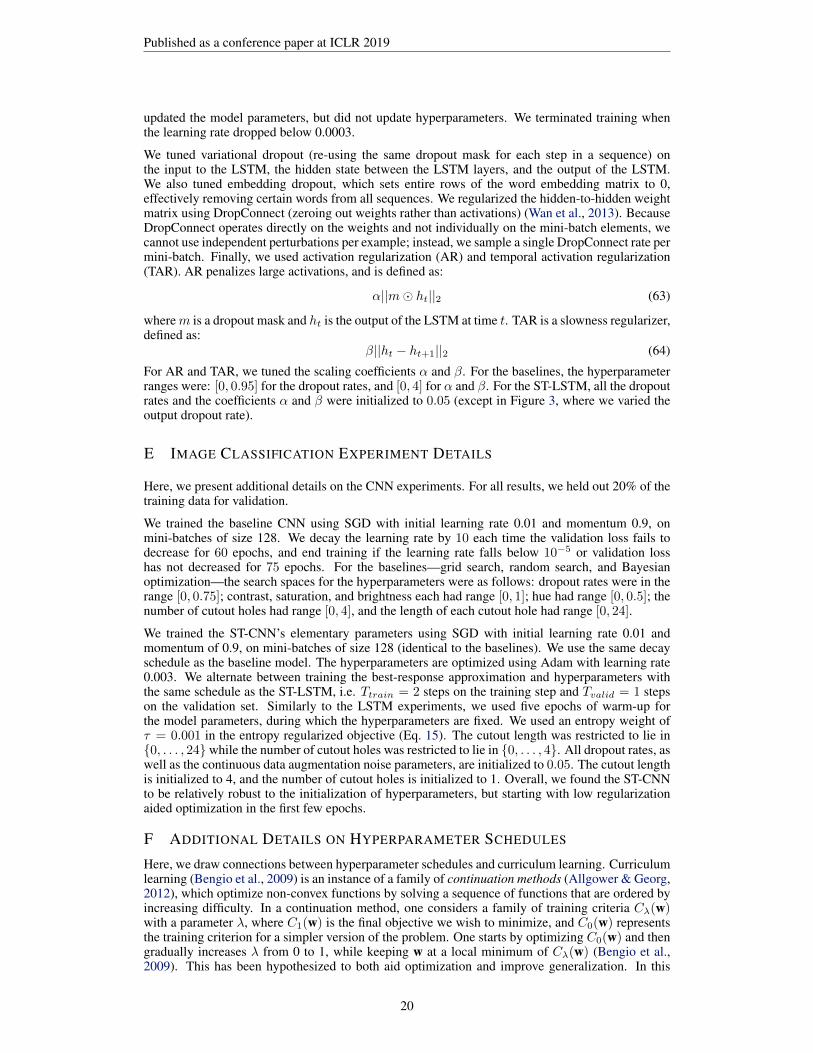
section, we explore how hyperparameter schedules implement a form of curriculum learning; forexample, a schedule that increases dropout over time increases stochasticity, making the learningproblem more difficult. We use the results of grid searches to understand the effects of differenthyperparameter settings throughout training, and show that greedy hyperparameter schedules canoutperform fixed hyperparameter values.

First, we performed a grid search over 20 values each of input and output dropout, and measured thevalidation perplexity in each epoch. Figure 7 shows the validation perplexity achieved by differentcombinations of input and output dropout, at various epochs during training. We see that at the startof training, the best validation loss is achieved with small values of both input and output dropout.As we train for more epochs, the best validation performance is achieved with larger dropout rates.

0.0 0.1 0.2 0.3 0.4 0.5 0.6 0.7 0.8 0.9Input Dropout

0.0

0.1

0.2

0.3

0.4

0.5

0.6

0.7

0.8

0.9

Outp

ut D

ropo

ut

Epoch 1

(a)

0.0 0.1 0.2 0.3 0.4 0.5 0.6 0.7 0.8 0.9Input Dropout

0.0

0.1

0.2

0.3

0.4

0.5

0.6

0.7

0.8

0.9

Outp

ut D

ropo

ut

Epoch 10

(b)

0.0 0.1 0.2 0.3 0.4 0.5 0.6 0.7 0.8 0.9Input Dropout

0.0

0.1

0.2

0.3

0.4

0.5

0.6

0.7

0.8

0.9

Outp

ut D

ropo

ut

Epoch 25

(c)

Figure 7: Validation performance of a baseline LSTM given different settings of input and outputdropout, at various epochs during training. (a), (b), and (c) show the validation performance on PTB givendifferent hyperparameter settings, at epochs 1, 10, and 25, respectively. Darker colors represent lower (better)validation perplexity.

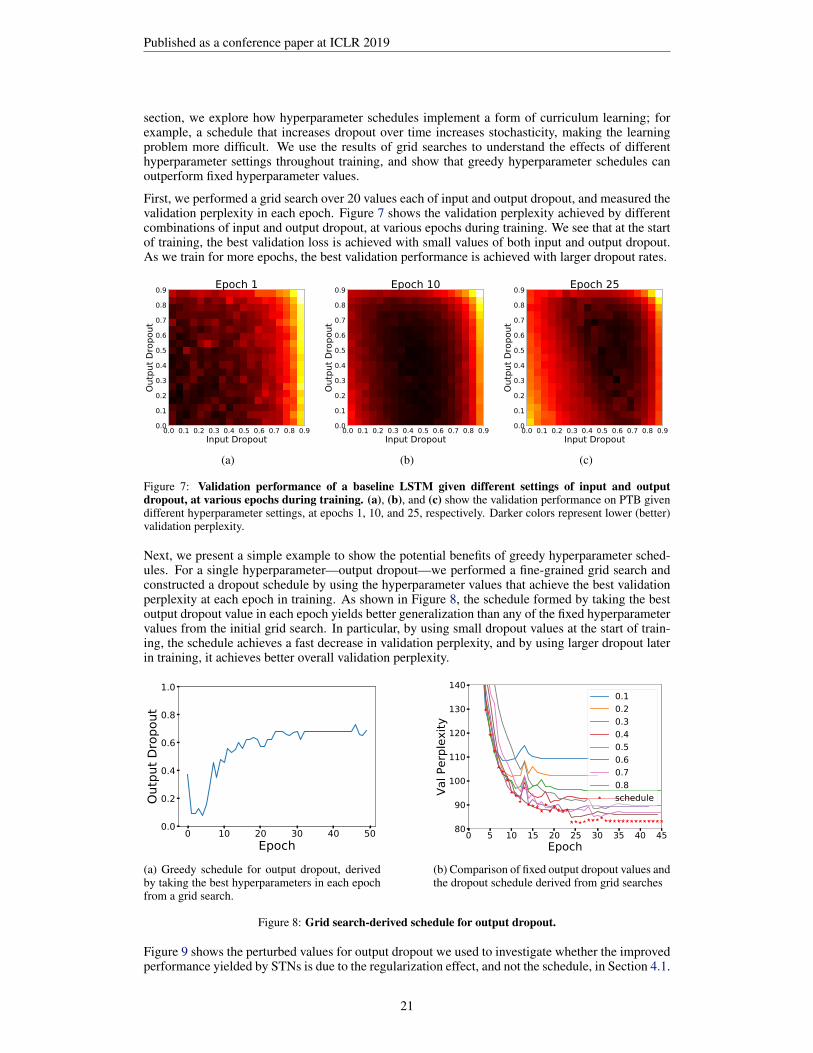
Next, we present a simple example to show the potential benefits of greedy hyperparameter sched-ules. For a single hyperparameter—output dropout—we performed a fine-grained grid search andconstructed a dropout schedule by using the hyperparameter values that achieve the best validationperplexity at each epoch in training. As shown in Figure 8, the schedule formed by taking the bestoutput dropout value in each epoch yields better generalization than any of the fixed hyperparametervalues from the initial grid search. In particular, by using small dropout values at the start of train-ing, the schedule achieves a fast decrease in validation perplexity, and by using larger dropout laterin training, it achieves better overall validation perplexity.

0 10 20 30 40 50Epoch

0.0

0.2

0.4

0.6

0.8

1.0

Outp

ut D

ropo

ut

(a) Greedy schedule for output dropout, derivedby taking the best hyperparameters in each epochfrom a grid search.

0 5 10 15 20 25 30 35 40 45Epoch

80

90

100

110

120

130

140

Val P

erpl

exity

0.10.20.30.40.50.60.70.8schedule

(b) Comparison of fixed output dropout values andthe dropout schedule derived from grid searches

Figure 8: Grid search-derived schedule for output dropout.

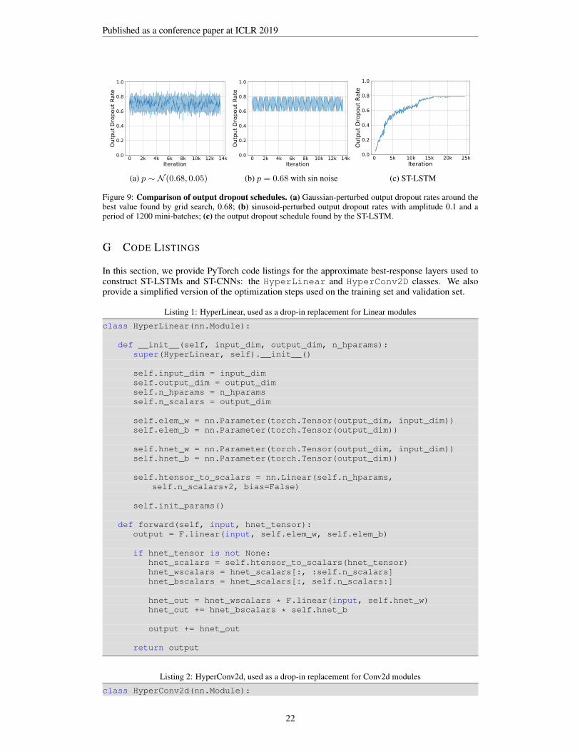
Figure 9 shows the perturbed values for output dropout we used to investigate whether the improvedperformance yielded by STNs is due to the regularization effect, and not the schedule, in Section 4.1.

21


0 2k 4k 6k 8k 10k 12k 14kIteration

0.0

0.2

0.4

0.6

0.8

1.0

Outp

ut D

ropo

ut R

ate

(a) p ∼ N (0.68, 0.05)

0 2k 4k 6k 8k 10k 12k 14kIteration

0.0

0.2

0.4

0.6

0.8

1.0

Outp

ut D

ropo

ut R

ate

(b) p = 0.68 with sin noise

0 5k 10k 15k 20k 25kIteration

0.0

0.2

0.4

0.6

0.8

1.0

Outp

ut D

ropo

ut R

ate

(c) ST-LSTM

Figure 9: Comparison of output dropout schedules. (a) Gaussian-perturbed output dropout rates around thebest value found by grid search, 0.68; (b) sinusoid-perturbed output dropout rates with amplitude 0.1 and aperiod of 1200 mini-batches; (c) the output dropout schedule found by the ST-LSTM.

G CODE LISTINGS

In this section, we provide PyTorch code listings for the approximate best-response layers used toconstruct ST-LSTMs and ST-CNNs: the HyperLinear and HyperConv2D classes. We alsoprovide a simplified version of the optimization steps used on the training set and validation set.

Listing 1: HyperLinear, used as a drop-in replacement for Linear modules

class HyperLinear(nn.Module):

def __init__(self, input_dim, output_dim, n_hparams):super(HyperLinear, self).__init__()

self.input_dim = input_dimself.output_dim = output_dimself.n_hparams = n_hparamsself.n_scalars = output_dim

self.elem_w = nn.Parameter(torch.Tensor(output_dim, input_dim))self.elem_b = nn.Parameter(torch.Tensor(output_dim))

self.hnet_w = nn.Parameter(torch.Tensor(output_dim, input_dim))self.hnet_b = nn.Parameter(torch.Tensor(output_dim))

self.htensor_to_scalars = nn.Linear(self.n_hparams,self.n_scalars*2, bias=False)

self.init_params()

def forward(self, input, hnet_tensor):output = F.linear(input, self.elem_w, self.elem_b)

if hnet_tensor is not None:hnet_scalars = self.htensor_to_scalars(hnet_tensor)hnet_wscalars = hnet_scalars[:, :self.n_scalars]hnet_bscalars = hnet_scalars[:, self.n_scalars:]

hnet_out = hnet_wscalars * F.linear(input, self.hnet_w)hnet_out += hnet_bscalars * self.hnet_b

output += hnet_out

return output

Listing 2: HyperConv2d, used as a drop-in replacement for Conv2d modules

class HyperConv2d(nn.Module):

22


def __init__(self, in_channels, out_channels, kernel_size, padding,num_hparams,stride=1, bias=True):super(HyperConv2d, self).__init__()

self.in_channels = in_channelsself.out_channels = out_channelsself.kernel_size = kernel_sizeself.padding = paddingself.num_hparams = num_hparamsself.stride = stride

self.elem_weight = nn.Parameter(torch.Tensor(out_channels, in_channels, kernel_size, kernel_size))

self.hnet_weight = nn.Parameter(torch.Tensor(out_channels, in_channels, kernel_size, kernel_size))

if bias:self.elem_bias = nn.Parameter(torch.Tensor(out_channels))self.hnet_bias = nn.Parameter(torch.Tensor(out_channels))

else:self.register_parameter(’elem_bias’, None)self.register_parameter(’hnet_bias’, None)

self.htensor_to_scalars = nn.Linear(self.num_hparams, self.out_channels*2, bias=False)

self.elem_scalar = nn.Parameter(torch.ones(1))

self.init_params()

def forward(self, input, htensor):"""Arguments:

input (tensor): size should be (B, C, H, W)htensor (tensor): size should be (B, D)

"""output = F.conv2d(input, self.elem_weight, self.elem_bias,

padding=self.padding,stride=self.stride)

output *= self.elem_scalarif htensor is not None:

hnet_scalars = self.htensor_to_scalars(htensor)hnet_wscalars = hnet_scalars[:,

:self.out_channels].unsqueeze(2).unsqueeze(2)hnet_bscalars = hnet_scalars[:, self.out_channels:]

hnet_out = F.conv2d(input, self.hnet_weight,padding=self.padding,stride=self.stride)

hnet_out *= hnet_wscalarsif self.hnet_bias is not None:

hnet_out += (hnet_bscalars *self.hnet_bias).unsqueeze(2).unsqueeze(2)

output += hnet_outreturn output

def init_params(self):n = self.in_channels * self.kernel_size * self.kernel_sizestdv = 1. / math.sqrt(n)self.elem_weight.data.uniform_(-stdv, stdv)self.hnet_weight.data.uniform_(-stdv, stdv)if self.elem_bias is not None:

self.elem_bias.data.uniform_(-stdv, stdv)self.hnet_bias.data.uniform_(-stdv, stdv)

23


self.htensor_to_scalars.weight.data.normal_(std=0.01)

Listing 3: Stylized optimization step on the training set for updating elementary parameters

# Perturb hyperparameters around current value in unconstrained# parametrization.batch_htensor = perturb(htensor, hscale)

# Apply necessary reparametrization of hyperparameters.hparam_tensor = hparam_transform(batch_htensor)

# Sets data augmentation hyperparameters in the data loader.dataset.set_hparams(hparam_tensor)

# Get next batch of examples and apply any input transformation# (e.g. input dropout) as dictated by the hyperparameters.images, labels = next_batch(dataset)images = apply_input_transform(images, hparam_tensor)

# Run everything through the model and do gradient descent.pred = hyper_cnn(images, batch_htensor, hparam_tensor)xentropy_loss = F.cross_entropy(pred, labels)xentropy_loss.backward()cnn_optimizer.step()

Listing 4: Stylized optimization step on the validation set for updating hyperparameters/noise scale

# Perturb hyperparameters around current value in unconstrained# parametrization, so we can assess sensitivity of validation# loss to the scale of the noise.batch_htensor = perturb(htensor, hscale)

# Apply necessary reparametrization of hyperparameters.hparam_tensor = hparam_transform(batch_htensor)

# Get next batch of examples and run through the model.images, labels = next_batch(valid_dataset)pred = hyper_cnn(images, batch_htensor, hparam_tensor)xentropy_loss = F.cross_entropy(pred, labels)

# Add extra entropy weight term to loss.entropy = compute_entropy(hscale)loss = xentropy_loss - args.entropy_weight * entropyloss.backward()

# Tune the hyperparameters.hyper_optimizer.step()

# Tune the scale of the noise applied to hyperparameters.scale_optimizer.step()

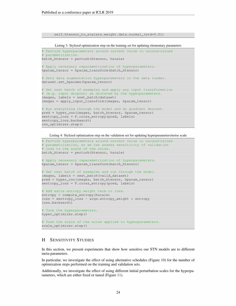
H SENSITIVITY STUDIES

In this section, we present experiments that show how sensitive our STN models are to differentmeta-parameters.

In particular, we investigate the effect of using alternative schedules (Figure 10) for the number ofoptimization steps performed on the training and validation sets.

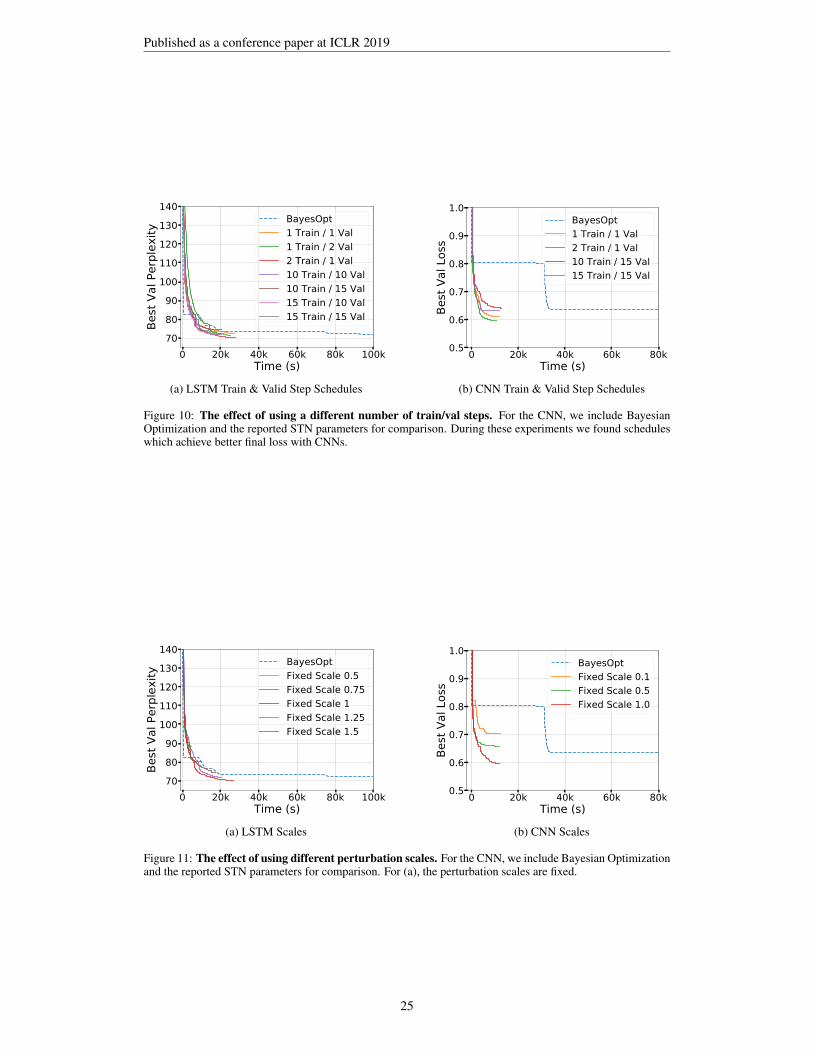
Additionally, we investigate the effect of using different initial perturbation scales for the hyperpa-rameters, which are either fixed or tuned (Figure 11).

24


0 20k 40k 60k 80k 100kTime (s)

708090

100110120130140

Best

Val

Per

plex

ity

BayesOpt1 Train / 1 Val1 Train / 2 Val2 Train / 1 Val10 Train / 10 Val10 Train / 15 Val15 Train / 10 Val15 Train / 15 Val

(a) LSTM Train & Valid Step Schedules

0 20k 40k 60k 80kTime (s)

0.5

0.6

0.7

0.8

0.9

1.0

Best

Val

Los

s

BayesOpt1 Train / 1 Val2 Train / 1 Val10 Train / 15 Val15 Train / 15 Val

(b) CNN Train & Valid Step Schedules

Figure 10: The effect of using a different number of train/val steps. For the CNN, we include BayesianOptimization and the reported STN parameters for comparison. During these experiments we found scheduleswhich achieve better final loss with CNNs.

0 20k 40k 60k 80k 100kTime (s)

708090

100110120130140

Best

Val

Per

plex

ity

BayesOptFixed Scale 0.5Fixed Scale 0.75Fixed Scale 1Fixed Scale 1.25Fixed Scale 1.5

(a) LSTM Scales

0 20k 40k 60k 80kTime (s)

0.5

0.6

0.7

0.8

0.9

1.0

Best

Val

Los

s

BayesOptFixed Scale 0.1Fixed Scale 0.5Fixed Scale 1.0

(b) CNN Scales

Figure 11: The effect of using different perturbation scales. For the CNN, we include Bayesian Optimizationand the reported STN parameters for comparison. For (a), the perturbation scales are fixed.

25

self-t networks b optimization of …

Documents