self-similar fold evolution under prescribed end-shortening
TRANSCRIPT
P1: FJD/FJN P2: FJD/LNH QC: FJD/FGE T1: FJD
Mathematical Geology [mg] 860 September 16, 1999 10:41 Style file version June 30, 1999
Mathematical Geology, Vol. 31, No. 8, 1999
Self-Similar Fold Evolution Under PrescribedEnd-Shortening1
Chris J. Budd,2 Giles W. Hunt,3 and Mark A. Peletier4
The evolution of single-layer folds under prescribed end-shortening conditions displays folds of varyingwavelength. We investigate a simple model of this kind and characterize the long-term behaviour of foldprofiles. In particular we determine the evolution of the axial load and the variation of the wavelength,and we show that fold profiles are highly self-similar.
KEY WORDS: long-term asymptotics, fold characterization, variable wave-length, viscous winklerfoundation, viscous halfspace.
INTRODUCTION
The variety of folding patterns in geological strata has always inspired a particularfascination. It seems intuitively obvious that some mechanism should be responsi-ble for the selection between different observed forms; but although many modelsand mechanisms have been proposed, there is a widespread feeling that the processof folding is still not well understood. For more than fifty years, analytical mod-els have been proposed as a means of understanding folding. Single-layer foldingmodels mostly take the form of a thin layer embedded in a homogeneous matrixsubject to compression parallel to the layer.
The creation—and subsequent deformation—of a fold necessarily spans acertain time, and that it therefore is natural to think of the process as anevolutionfrom the straight layer (probably with perturbations) via creation, amplification,and finally freezing to the form that is eventually observed. From this perspective
1Received 9 June 1998; accepted 12 January 1999.2Department of Mathematical Sciences, University of Bath, Bath BA2 7AY, United Kingdom. e-mail:C. J. [email protected]
3Department of Mechanical Engineering, University of Bath. e-mail: G. W. [email protected] of Mathematical Sciences and Mechanical Engineering, University of Bath. Currentaddress: Centrum voor Wiskunde en Informatica (CWI), P. O. Box 94079, 1090 GB Amsterdam.e-mail: Mark. [email protected]
989
0882-8121/99/1100-0989$16.00/1C© 1999 International Association for Mathematical Geology
P1: FJD/FJN P2: FJD/LNH QC: FJD/FGE T1: FJD
Mathematical Geology [mg] 860 September 16, 1999 10:41 Style file version June 30, 1999
990 Budd, Hunt, and Peletier
it is interesting to note that many of the more traditional models—notably the“dominant wavelength” family—retain only a caricature of this evolution in theform of a comparison of different growth rates. There is clearly much to be gainedfrom a faithful modeling of the complete evolution process.
In the modeling of folding as an evolution process one issue in particular hasa marked influence on the response. The traditional formulation considers foldevolution under a prescribed layer-parallel load. In recent years, however, it hasbecome clear that fold evolution under prescribed end-shortening (or total strain)may be more realistic (M¨uhlhaus, Hobbs, and Ord, 1994; Hunt, M¨uhlhaus, andWhiting, 1996; Whiting, 1996; Whiting and Hunt, 1997). The purpose of thispaper is to analyze and extend simple models of this kind, place the results ona mathematical footing, and generally provide new insights. Where appropriate,numerical results are used to illustrate these. Notably our findings of (approximate)self-similarity in models of single-layer folding seem to be new.
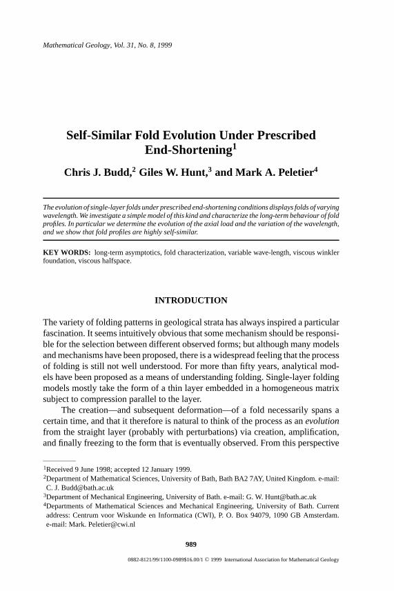
We model single-layer folding by an unbounded elastic layer embedded in aviscous matrix (Fig. 1).
The constitutional laws are linear, and small deflections are assumed. Theequations governing this model are (after rescaling)
ut + uxxxx+ Puxx = 0 −∞ < x <∞ (1)
1
2
∫ ∞−∞
u2x dx = g(t) (2)
The first equation is a force balance, whereu= u(x, t) is the vertical displacementof the layer,x the horizontal distance measured along the layer,P= P(t) the axial(layer-parallel) load, andux is assumed small. Subscripts denote differentiation.Equation (2) describes the condition of prescribed end-shortening. The functiong(t) is given; with tectonic compression in mind a typical functiong(t) might bea+ bt. Note that prescribing the end-shortening implies thatP is free and needsto be determined as part of the solution (see the next section for the details ofthe derivation of these equations). We show that for all localized initial data thisequation has a unique, localized, globally attracting self-similar behaviour.
Figure 1. An elastic layer on a viscous bedding.
P1: FJD/FJN P2: FJD/LNH QC: FJD/FGE T1: FJD
Mathematical Geology [mg] 860 September 16, 1999 10:41 Style file version June 30, 1999
Self-Similar Fold Evolution 991
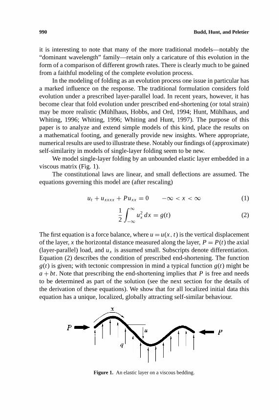
Figure 2. Evolution of the deformed layer.
The equation for the layer itself is completely linear; the only nonlinearity inthe problem is the constraint (2). However, this constraint has profound effects onthe behaviour of the model. We mention a number of these effects below.
1.Localized folds remain localized.A consequence of the evolutionary aspectof the model is that a localized initial perturbation gives rise to a localized sub-sequent fold evolution. Figure 2 shows an example of how an initial perturbationevolves for a linearly increasing end-shortening functiong (see the companionpaper by Budd and Peletier (1998) for the details of the numerical calculationsshown in this paper).
The unboundedness of the layer has nothing to do with this property: longbut finite layers should evolve in a similar way to unbounded layers, providedthe perturbation itself is localized, and up to the time when the folds reach theends of the layer. In a similar vein, two localized perturbations far apart shouldevolve independently until the spreading of the folds makes them interfere witheach other.
2.Wavelength and axial load change through time.Whilst the profiles of Fig-ure 2 remain localized, there is a clear increase in wavelength as time increases.This is coupled to a marked decrease inP (Fig. 3A).
The case of constant load in this model setup (small deflections, an elastic layeron a viscous foundation) was studied first by Biot (1965). He found a relationshipbetweenP and the wavelengthL of the type
L = c√P
wherec is a constant depending on the layer thickness and the elastic parametersof the layer (in the case of Equation (1), where coefficients have been rescaled,c= 2π ). Figure 3B shows the productL
√P for a long-term calculation. While
there is a clear discrepancy initially, for large timesL√
P approaches the value2π , independent of initial conditions. This effect is explained simply: as timeadvances,P varies less rapidly, and Biot’s approximation by a constant load gainsin accuracy. Note however the time scale on which this convergence takes place.

P1: FJD/FJN P2: FJD/LNH QC: FJD/FGE T1: FJD
Mathematical Geology [mg] 860 September 16, 1999 10:41 Style file version June 30, 1999
992 Budd, Hunt, and Peletier
Figure 3. Evolution of loadP vs. time and scaled wavelengthL√
P for aconstant end-shortening evolution.
This variation in wavelength demonstrates an important property of pre-scribed end-shortening models (see also M¨uhlhaus, Hobbs, and Ord, 1994; Whitingand Hunt, 1997; Whiting, 1996):there is no dominant wavelengthvalid over alltimescales.
3.The long-term evolution is self-similar.As shown in Figure 4A, calculatedprofiles show a simultaneous increase in amplitude and in wavelength as timeadvances. Under a suitable rescaling, however—see Figure 5—the differencesare strongly reduced. In the analysis later in this paper, we determine the exactasymptotic behavior in the limitt→∞. For instance, in the case of constantend-shortening [g(t)=a> 0] we have
u(x, t) ∼ A√
at1/8
[log t ]1/4e−y2/6 logt cosy (3)
wherey= Bxt−1/4[log t ]1/4 andA andB are constants. Figure 6 shows a numer-ically calculated solution compared to the asymptotic profile (3).
Note that on most time scales logt can be considered constant in comparisonto powers oft , reducing (3) to
u(x, t) ∼ A√
a t1/8e−cy2cosy (4)
with y= Bxt−1/4 for slowly varying functionsA, B, andc.

P1: FJD/FJN P2: FJD/LNH QC: FJD/FGE T1: FJD
Mathematical Geology [mg] 860 September 16, 1999 10:41 Style file version June 30, 1999
Self-Similar Fold Evolution 993
Figure 4. Evolution of the solution profileu under constantend-shortening.
This formula shows that profiles are self-similar in the long term: at differenttimes the profiles have the same form, but rescaled (“vertically” by a factort1/8,and “horizontally” by a factort1/4). Again we see in this long-term behavior thatthe wavelength continues to increase and tends to infinity in the limitt→∞.

P1: FJD/FJN P2: FJD/LNH QC: FJD/FGE T1: FJD
Mathematical Geology [mg] 860 September 16, 1999 10:41 Style file version June 30, 1999
994 Budd, Hunt, and Peletier
Figure 5. The same evolution as Figure 4A, but presented inself-similar variables. In these variables, an exact self-similarsolution would appear constant.
Figure 6. Comparison between the numerically calculated so-lution and the asymptotic profile (constant end-shortening). Thescales have been chosen in accordance with Equation (14).
4. Independence of initial perturbations.An important consequence of (3),one that merits separate mentioned, is that the long-term behavior has a genericform and is therefore independent of the form of the initial perturbation.
There are a number of results in the literature that focus on the relationshipbetween the shape of the initial perturbation and that of the subsequent folds(Cobbold, 1975; Cobbold, 1977; Williams, Lewis, and Zienkiewicz, 1978; Abbasi

P1: FJD/FJN P2: FJD/LNH QC: FJD/FGE T1: FJD
Mathematical Geology [mg] 860 September 16, 1999 10:41 Style file version June 30, 1999
Self-Similar Fold Evolution 995
and Mancktelow, 1990; Abbasi and Mancktelow, 1992; Mancktelow and Abbasi,1992; Zhang and others, 1996). The independence of initial data mentioned abovedoes not contradict these findings, but merely indicates that the correspondencebetween initial form and subsequent folds weakens as the folds evolve.
This is illustrated by Figures 4A and 4B. The initial stages of fold developmentare clearly different in the two cases, but at larger times there is a strong similarity.Note that although the early stages of fold development in Figure 4B do notresemble the generic fold shape that appears in the later stages, the increase inwavelength can be observed almost immediately.
5. The importance of (geometric) large-deflection effects may be either smallor large, depending on the end-shortening functiong(t). The derivation of (1) and(2) involves the assumption that the limb angle is small. As mentioned above, thelarge-time behavior underconstantend-shortening is (roughly) of the form
u(x, t) ∼ t1/8 f (xt−1/4) (5)
The limb angle is related to the derivativeux, which will have a long-term form,
ux(x, t) ∼ t−1/8 f ′(xt−1/4)
by the chain rule. Consequently, the maximum of|ux| overx ∈R is equal to
t−1/8 maxy∈R| f ′(y)|
and therefore tends to zero ast→∞. Hence the assumption thatux is smallbecomes increasingly accurate in the long-term limit. We expect therefore that ageometrically nonlinear model will share the same long-term behavior.
The situation is different for a linearly increasing end-shortening. Here thelong-term behavior takes the form
u(x, t) ∼ t5/8 f (xt−1/4)
so that
ux(x, t) ∼ t3/8 f ′(xt−1/4)
implying that the maximum limb anglegrows in time. Consequently, the small-deflection approximation becomes less accurate in time, and we expect the two todiffer strongly in the limitt→∞.
In the sections that follow, we describe the model, discuss self-similar solu-tions, and investigate the full long-term behavior of the solutions. Our techniques

P1: FJD/FJN P2: FJD/LNH QC: FJD/FGE T1: FJD
Mathematical Geology [mg] 860 September 16, 1999 10:41 Style file version June 30, 1999
996 Budd, Hunt, and Peletier
are based heavily on use of the continuous Fourier transform on the real line, and inthe Appendix we state a number of properties of this transform. Most of the detailsof proofs have been left out. The interested reader can find a rigorous treatment ofthese results in Budd and Peletier (1998).
THE MODEL
We consider a thin linear elastic layer on a linear viscous bedding, as inFigure 1. Assuming small deflection, the equation for the vertical deflectionuis
Duxxxx+ Puxx + q = 0 −∞ < x <∞, t > 0 (6)
whereq is the bedding force andP= P(t) the axial load on the elastic layer, andx is the distance along the layer (arc length). The bending stiffnessD is equal toEh3/12(1− ν2), whereh is the thickness of the layer. Note that we consider thisequation on the whole real line.
We consider two types of foundation: (a) a linear viscous Winkler foundation,and (b) a linear viscous halfspace. For the Winkler foundation the forceq is simplygiven byq= ηut (η is the viscosity); for the halfspaceq= 4ηH (uxt) (Biot, 1965,p. 419), whereH is the Hilbert transform (see the Appendix for the definitionof the Fourier and Hilbert transforms). By rescaling the various coefficients, thisleads to
(Winkler foundation) ut + uxxxx+ Puxx = 0 (7)
and
(halfspace) H (uxt)+ uxxxx+ Puxx = 0 (8)
The reasons for considering two different foundations are twofold. First, the Win-kler foundation is simpler in concept and implementation, while the viscous half-space is closer to reality. Second, the fact that the long-term results are similarin nature for the two foundations indicates that only the viscous quality of thefoundation is of importance for the long-term behavior; other properties play aminor role.
As mentioned above,P is not prescribed; instead, the total end-shortening issupposed to be equal to a prescribed function of time. By using a small-deflectionapproximation, this can be modeled as
1
2
∫ ∞−∞
u2x(x) dx = g(t) t ≥ 0 (9)

P1: FJD/FJN P2: FJD/LNH QC: FJD/FGE T1: FJD
Mathematical Geology [mg] 860 September 16, 1999 10:41 Style file version June 30, 1999
Self-Similar Fold Evolution 997
Here the functiong(t) is the prescribed amount of end-shortening. If we supplementthese equations with an initial condition,
u(x, 0)= u0(x) −∞ < x <∞ (10)
and assume thatu0 satisfies (9)—i.e.,∫
u20x = g(0)—then this problem has a unique
solution (u, P). Note thatu is a function ofx andt , but P is a function of timeonly.
LARGE-TIME BEHAVIOR I: SELF-SIMILAR SOLUTIONS
We can make an educated guess of the large-time behavior of solutions by con-sidering the scaling invariance of the equations. Taking as an example the Winklerfoundation model with a constant end-shortening [constantg(t)], Equation (7) isinvariant under the scaling
x→ λ1/4x, t → λt, P→ λ−1/2P
and so we might expect to find self-similar solutions that scale accordingly, i.e.,solutions of the form
u(x, t) = t1/8 f (xt−1/4), P(t) = Qt−1/2 (11)
The factort1/8 is chosen as to satisfy the constraint:∫u2
x(x, t) dx =∫
[t−1/8 f ′(xt−1/4)]2 dx
=∫
f ′(xt−1/4)2 dxt−1/4 =∫
f ′(ξ )2 dξ
where the primes denote differentiation with respect to the self-similar variableξ = xt−1/4. If a functionu of the form (11) satisfies Equation (7), then the profilef solves the ordinary differential equation
f ′′′′ + Q f ′′ + 1
8f − 1
4ξ f ′ = 0 −∞ < ξ <∞ (12)
and the constraint
1
2
∫f ′(ξ )2 dξ = g (constant) (13)

P1: FJD/FJN P2: FJD/LNH QC: FJD/FGE T1: FJD
Mathematical Geology [mg] 860 September 16, 1999 10:41 Style file version June 30, 1999
998 Budd, Hunt, and Peletier
However, the system of Equations (12) and (13) has no solutions. This canbe seen from translating the equation to the Fourier domain. Applying the Fouriertransform to Equation (12) we find, writingf for f (ω),
ω4 f − Qω2 f + 1
8f − 1
4√
2πξ ∗ (iω f ) = 0
Using ξ = i√
2πδ′, whereδ is the Dirac delta function,
[ξ ∗ (iω f )](ω) = −√
2πδ′ ∗ (ω f )
= −√
2πδ ∗ (ω f )′
= −√
2π (ω f )′
= −√
2π ( f + ω f′)
Here f′(ω)= d/dω f (ω). We find that f satisfies
f
(ω4− Qω2+ 3
8
)+ 1
4ω f′ = 0
which can also be written as
f′
f= −3
2ω−1− 4ω3+ 4Qω
Close toω= 0, the behavior off is given by the first term on the right-hand side,so that if f is nonzero, then
f (ω) ∼ |ω|−3/2 asω→ 0
Hence ∫f ′(ξ )2 dξ =
∫ω2| f (ω)|2 dω = ∞
implying that f cannot satisfy condition (13). Hence, there are no self-similarsolutions of the exact form (11).
The nonexistence of exact self-similar solutions implies that solutions cannothave a long-term behavior of self-similar form. However, the underlying scalingproperties of the problem continue to drive the evolution along the lines of self-similarity. The result is a long-term behavior that isapproximately self-similar.

P1: FJD/FJN P2: FJD/LNH QC: FJD/FGE T1: FJD
Mathematical Geology [mg] 860 September 16, 1999 10:41 Style file version June 30, 1999
Self-Similar Fold Evolution 999
LARGE-TIME BEHAVIOR II: APPROXIMATE SELF-SIMILARITY
The actual large-time behavior follows the self-similar scaling closely witha small (logarithmic) correction. We will discuss this now in some detail. For theprecise statement of our result, and to combine several types of constraint functionsg, we set
g(t) = a+ btγ , a, γ ≥ 0, b > 0
The notationα∼β denotesα/β→ 1 ast→∞.
Theorem 1 (Winkler foundation). Let u be the solution of Equations (7) and (9)with initial datum u0. As t→∞,
P(t) ∼ 2−1/2t−1/2[(γ + 3/4) logt ]1/2
and if
u(x, t) = P−1/4g1/2v(x P1/2, t) (14)
then
v(y, t) ∼√
2[π (γ + 3/4) logt ]−1/4e−y2/8(γ+3/4) logt cosy (15)
Theorem 2 (Halfspace).Let u be the solution of Equations (8) and (9) with initialdatum u0. As t→∞,
P(t) ∼ 2−4/3t−2/3[(γ + 3/4) logt ]1/2
and if u(x, t)= P−1/4g1/2v(x P1/2, t), then
v(y, t) ∼ 23/4[3π (1+ γ ) log t ]−1/4e−y2/3(1+γ ) log t cosy
Remark. Depending on the time scales involved, the expressions above might besimplified by considering the logarithms in these expressions as slowly varyingwith respect to the powers oft . If so, then we find on combining (14) and (15) thatfor the Winkler foundation of fold profiles take the asymptotic form
u(x, t) ∼ A√
bt1/8+γ /2e−cy2cosy
wherey= Bxt−1/4, for some slowly varying functionsA, B, c> 0. Similarly, thehalfspace profiles take the form
P1: FJD/FJN P2: FJD/LNH QC: FJD/FGE T1: FJD
Mathematical Geology [mg] 860 September 16, 1999 10:41 Style file version June 30, 1999
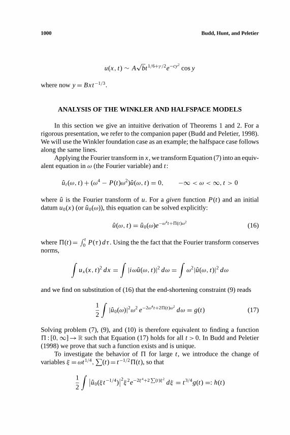
1000 Budd, Hunt, and Peletier
u(x, t) ∼ A√
bt1/6+γ /2e−cy2cosy
where nowy= Bxt−1/3.
ANALYSIS OF THE WINKLER AND HALFSPACE MODELS
In this section we give an intuitive derivation of Theorems 1 and 2. For arigorous presentation, we refer to the companion paper (Budd and Peletier, 1998).We will use the Winkler foundation case as an example; the halfspace case followsalong the same lines.
Applying the Fourier transform inx, we transform Equation (7) into an equiv-alent equation inω (the Fourier variable) andt :
ut (ω, t)+ (ω4− P(t)ω2)u(ω, t) = 0, −∞ < ω <∞, t > 0
whereu is the Fourier transform ofu. For agiven function P(t) and an initialdatumu0(x) (or u0(ω)), this equation can be solved explicitly:
u(ω, t) = u0(ω)e−ω4t+5(t)ω2
(16)
where5(t)= ∫ t0 P(τ ) dτ . Using the the fact that the Fourier transform conserves
norms, ∫ux(x, t)2 dx =
∫|iωu(ω, t)|2 dω =
∫ω2|u(ω, t)|2 dω
and we find on substitution of (16) that the end-shortening constraint (9) reads
1
2
∫|u0(ω)|2ω2 e−2ω4t+25(t)ω2
dω = g(t) (17)
Solving problem (7), (9), and (10) is therefore equivalent to finding a function5 : [0,∞]→R such that Equation (17) holds for allt > 0. In Budd and Peletier(1998) we prove that such a function exists and is unique.
To investigate the behavior of5 for large t , we introduce the change ofvariablesξ =ωt1/4,
∑(t)= t−1/25(t), so that
1
2
∫ ∣∣u0(ξ t−1/4)∣∣2ξ2e−2ξ4+2
∑(t)ξ2
dξ = t3/4g(t) =: h(t)

P1: FJD/FJN P2: FJD/LNH QC: FJD/FGE T1: FJD
Mathematical Geology [mg] 860 September 16, 1999 10:41 Style file version June 30, 1999
Self-Similar Fold Evolution 1001
We expect that∑
(t)→∞ ast→∞. Since thenξ2e−2ξ4+2∑
(t)ξ2localizes around
ξ = 0, one can expect that only the valueu0(0) is important for larget . This leadsto
1
2
∫ξ2e−2ξ4+2
∑(t)ξ2
dξ = |u0(0)|−2h(t)
providedu0(0) 6= 0. If we define
F(y) =∫ξ2e−2ξ4+2yξ2
dξ
then the function∑
(t) satisfies∑(t) = F−1
(2|u0(0)|−2h(t)
)and hence we only need to determine the behavior ofF(y) for largey, in order toknow the long-term behavior of
∑and consequently5 andP. Watson’s Lemma
(Theorem 7.1 in Olver, 1974) gives an asymptotic expression forF(y):
F(y) ∼ 1
2√πyey2/2 or F−1(z) ∼
√2 logz
both in the limity, z→∞. Thus∑(t) ∼
√2 logh(t)
and sinceh(t)∼ ctγ+3/4 (with c= b if γ >0 andc=a+ b if γ = 0),∑(t) ∼
√2(γ + 3/4) logt ast →∞.
Transforming back we find that5(t)∼√2(γ + 3/4)t log t and
P(t) ∼ 1
2t−1/2
√2(γ + 3/4) logt ast →∞
This proves the first part of Theorem 1.To determine the long-term profile, we examine the Fourier spectrum of the
solution [given by (16)],
u(ω, t) = u0(ω)e−ω4t+5(t)ω2

P1: FJD/FJN P2: FJD/LNH QC: FJD/FGE T1: FJD
Mathematical Geology [mg] 860 September 16, 1999 10:41 Style file version June 30, 1999
1002 Budd, Hunt, and Peletier
The exponent−ω4t +5(t)ω2 has a maximum of5(t)2/4t at the valuesω=±√5(t)/2t . Since5∼√2(γ + 3/4)t log t , this maximum tends to infinity ast →∞. Consequently, the spectrumu is dominated by two large spikes at thesevalues ofω. The long-term behavior (15) is obtained by characterizing these spikesin a convenient way.
By the scaling law (21) the Fourier transform ofv is given by
v(ξ, t) = P3/4g−1/2u(ξP1/2, t) = P3/4g−1/2u0(ξP1/2)e−P2tξ4+5Pξ2
whereξ =ωP1/2. From the expressions forP and5 above we have5P/P2t ∼ 2,so that
−P2tξ4+ P5ξ2 ∼ −P2t(ξ4− 2ξ2) ast →∞ (18)
Here the effect of the transformation (14) can be seen clearly: where the maxima inthe spectrum ofu move toward the origin, in ˆv they move toward a fixed positionξ =±1. Since the important contribution in the Fourier spectrum comes from theregion around these maxima, we simplify by replacingξ4− 2ξ2 with a parabolacentered on the maximum and with similar curvature, i.e.,
ξ4− 2ξ2→ 4(ξ − 1)2− 1 forξ > 0 (19)
and
ξ4− 2ξ2→ 4(ξ + 1)2− 1 forξ < 0 (20)
To summarize, we claim that ˆv converges to
z(ξ, t) = α(t){e−β(t)[4(ξ−1)2−1] + e−β(t)[4(ξ+1)2−1]
}providedα andβ are chosen appropriately. It turns out (see Budd and Peletier,1998, for the details) that
β ∼ 1
2(γ + 3/4) logt and α ∼ u0(0)P3/4g−1/2
and these values lead to the result (15). Note that the asymptotic behavior ofβ
coincides exactly with that ofP2t , as is to be expected from (18), (19), and (20).
P1: FJD/FJN P2: FJD/LNH QC: FJD/FGE T1: FJD
Mathematical Geology [mg] 860 September 16, 1999 10:41 Style file version June 30, 1999
Self-Similar Fold Evolution 1003
CONCLUSION
We have developed a new model for localized folds in an elastic layer em-bedded in a viscous matrix. This model takes into account the viscous aspects ofthe evolution and an end-shortening constraint. Localized folds remain localized,but widen through evolution, and show a continuously increasing wavelength. Inaddition, we have completely characterized the long-term behavior of these foldsand the associated axial load.
This long-term behavior is expected to apply not only to the viscous founda-tion of this model, but also to foundations that are viscoelastic, and also, in somecases, to geometrically nonlinear models (as explained in the Introduction). How-ever, a long-term result begs the question of the short-term character of the model,and we hope to explore this question in the future. It should be noted that herethe material properties are not irrelevant, and the difference between a viscoelasticand a viscous foundation should be visible.
A different extension, one that is hinted at in recent geological literature(Muhlhaus, Sakaguchi, and Hobbs, n.d.), would be to consider not only the foun-dation but also the layer to be viscoelastic. This would change the large-timebehavior in a fundamental way, since the strain energy contained in the deformedlayer can then dissipate viscously both in the foundation and in the layer. The ratiobetween the two viscosities is expected to be of prime importance in such a model.
Again a different but equally interesting extension would consist in relaxingthe small-deflection hypothesis, resulting in a geometrically nonlinear model forthe layer. Numerical results by Whiting and Hunt (1997) show interesting behavior,especially for a relatively rapid increase in end-shortening. Here again, elasticproperties could be significant.
ACKNOWLEDGMENTS
The authors are grateful to the EPSRC for their funding of this project throughgrant GR/L17177 of the Applied Nonlinear Mathematics Initiative.
REFERENCES
Abbasi, M. R., and Mancktelow, N. S., 1990, The effect of initial perturbation shape and symmetry onfold development: J. Struct. Geol., v. 12, no. 2, p. 273–282.
Abbasi, M. R., and Mancktelow, N. S., 1992, Single layer buckle folding in non-linear materials—I.Experimental study of fold development from an isolated initial perturbation: J. Struct. Geol., v.14, p. 85–104.
Biot, M. A., 1965, Mechanics of Incremental Deformations: Wiley, New York, 504 p.

P1: FJD/FJN P2: FJD/LNH QC: FJD/FGE T1: FJD
Mathematical Geology [mg] 860 September 16, 1999 10:41 Style file version June 30, 1999
1004 Budd, Hunt, and Peletier
Budd, C. J., and Peletier, M. A., 1998, Approximate self-similarity in models of geological folding:Technical Report 98/09, University of Bath. SIAM J. Appl. Math., to appear.
Cobbold, P. R., 1975, Fold propatation in single embedded layers: Tectonophysics, v. 27, p. 333–351.Cobbold, P. R., 1977, Finite-element analysis of fold propagation—A problematic application?:
Tectonophysics, v. 38, p. 339–353.Hunt, G. W., Muhlhaus, H.-B., and Whiting, A. I. M., 1996, Evolution of localized folding for a thin
elastic layer in a softening visco-elastic medium: Pure Appl. Geophys., v. 146, p. 229–252.Mancktelow, N. S., and Abbasi, M. R., 1992, Single layer buckle folding in non-linear materials—II.
Comparison between theory and experiment: J. Struct. Geol., v. 14, p. 105–120.Muhlhaus, H.-B., Hobbs, B. E., and Ord, A., 1994, The role of axial constraints on the evolution of folds
in single layers,in H. J. Siriwardane and M. M. Zaman, eds., Computer Methods and Advancesin Geomechanics, Vol. 1: A. A. Balkema, Rotterdam, p. 223–231.
Muhlhaus, H.-B., Sakaguchi, H., and Hobbs, B. E., n.d., Evolution of 3d folds for a non-newtonianplate in a viscous medium: Proc. R. Soc. Lond., to appear.
Olver, F. W. J., 1974, Asymptotics and Special Functions: Academic Press, 572 p.Whiting, A. I. M., 1996, Localized Buckling of an Elastic Strut in a Viscoelastic Medium: unpublished
doctoral dissertation, Imperial College of Science, Technology and Medicine, London.Whiting, A. I. M., and Hunt, G. W., 1997, Evolution of nonperiodic forms in geological folds: J. Math.
Geology, v. 29, no. 5, p. 705–723.Williams, J. R., Lewis, R. W., and Zienkiewicz, O. C., 1978, A finite-element analysis of the role of
initial perturbations in the folding of a single viscous layer: Tectonophysics, v. 45, p. 187–200.Zhang, Y., Hobbs, B. E., Ord, A., and M¨uhlhaus, H.-B., 1996, Computer simulation of single-layer
buckling: J. Struct. Geol., v. 18, no. 5, p. 643–655.
APPENDIX: FOURIER ANALYSIS AND THE HILBERT TRANSFORM
The Fourier transform of a functionu :R→R is defined by
F(u)(w) = 1√2π
∫u(x)e−iωx dx
We also writeu(ω) for F(u)(ω). The inverse transform is
F−1(v)(x) = v(x) = 1√2π
∫v(ω)eiωx dω
This transform conservesL2-norms identically, that is∫|u(x)|2 dx =
∫|u(ω)|2 dω
and derivatives transform into polynomials:
u′(ω) = iωu(ω)
P1: FJD/FJN P2: FJD/LNH QC: FJD/FGE T1: FJD
Mathematical Geology [mg] 860 September 16, 1999 10:41 Style file version June 30, 1999
Self-Similar Fold Evolution 1005
The convolution product of two functionsf andg onR is defined by
( f ∗ g)(x) =∫R
f (y)g(x − y) dy
This product is symmetric inf andg, has the property
( f ∗ g)′ = f ′ ∗ g = f ∗ g′
and interacts with Fourier transforms in a simple way:
uv(ω) = 1√2π
(u ∗ v)(ω)
For convenience we also mention the scaling law
u(λx)(ω) = 1
λu(ω/λ) (21)
The Hilbert Transform of a functionu :R→R is defined as
H (u)(x) = 1
π
∫ ∞−∞
u(y)
x − ydy
where the integral should be taken as a principal value. There exists an elegantalternative formulation of the Hilbert Transform in terms of Fourier transforms:
H (u)(ω) = −i sgn(ω)u(ω)