Università degli Studi di Roma “La Sapienza”

Self-Optimized Radio Resource Management Techniques for LTE-A Local

Area Deployments

Claudio Stocchi

Master’s Thesis in

Telecommunication Engineering

ADVISOR CO-ADVISOR

Maria-Gabriella Di Benedetto Nicola Marchetti

Academic Year 2009/2010

– ii –

– iii –

Abstract

The high performance requirements defined by the International Telecommunication Union (ITU)

for next generation wireless networks, and the ever increasing customers demand for new advanced

services, pose great challenges to operators that have also to take care of their revenues. A possible

solution that in the last years has received particular interest, is the adoption of low-power and low-

cost base stations, named Femtocells, to be used in Local Area Deployments such as offices and

homes, serving only a few users. This new trend poses some problems, the most relevant being the

Inter-Cell Interference (ICI) management, that in a scenario with uncoordinated deployment of base

stations, such as in Local Area Deployment scenarios are supposed to be, become even trickier than

in macro cellular networks. In order to face the ICI problem, one promising solution is the adoption

of the Self-Organizing Networks (SON) concept, that in particular should be applied to the Radio

Resource Management (RRM) functionalities, in order to allow the base stations to autonomously

change their behavior and parameters according to changes in the surrounding environment.

This thesis proposes an algorithm for downlink transmissions ICI management in a Self-Optimized

fashion. In particular it is composed by a Flexible Spectrum Usage (FSU) mechanism, that allows

neighboring cells to coexist and share common spectrum pool in a flexible manner, and a Power

Control mechanism that principally aims to limit the global ICI level and guarantee good

performance even to users in bad conditions, while achieving high global performance. Moreover

the proposed algorithm adopts also a Self-Configuring capability, that allows autonomous initial

spectrum selection for the base stations.

– iv –

– v –

Acknowledgements

This report is the result of the Master’s Thesis work conducted at Aalborg University as a guest

student from University of Rome “La Sapienza”.

First of all I would like to thank my supervisor Nicola Marchetti, for the support given and the time

spent with me. In particular I would like to thank him for the autonomy and independence he gave

me in the thesis process, giving me the right suggestions but letting me do my choices since as he

said, referring to me, from the very first day I was here: “This is Your thesis, not mine”. I would

also like to thank my other supervisor, Neeli Rashmi Prasad, for her support and for giving me the

possibility to study in the CTIF S-COGITO laboratory.

A great appreciation goes also to my supervisor in Rome, Maria-Gabriella Di Benedetto who has

always encouraged and helped me to come here at Aalborg University allowing me to do one of the

most relevant experiences of my life, as a student and as a person.

– vi –

– vii –

Acronyms

3GPP 3rd Generation Partnership Project

AGW Access Gateway

BS Base Station

CAGR Compound Annual Growth Rate

CAPEX Capital Expenditure

CDF Cumulative Distribution Function

CP Cyclic Prefix

CQI Channel Quality Indicator

CSG Closed Subscriber Group

DL Downlink

DSL Digital Subscriber Line

E-UTRAN Evolved-UMTS Terrestrial Radio Access Network

eNB evolved Node-B

EPC Evolved Packet Core

EUL Enhanced Uplink

FD Frequency Domain

FDM Frequency Division Multiplexing

FSU Flexible Spectrum Usage

GERAN GSM EDGE Radio Access Network

GGSN Gateway GPRS Support Node

GSM Global System for Mobile Communications

HARQ Hybrid Automatic Repeat Request

HeNB Home evolved Node-B

HSPA High Speed Packet Access

HSDPA High Speed Downlink Packet Access

ICI Inter-Cell Interference

IMT-A International Mobile Telecommunications - Advanced

ISI Inter-Symbol Interference

ITU International Telecommunication Union

LOS Line Of Sight

LTE Long Term Evolution

LTE-A Long Term Evolution - Advanced

– viii –

MME Mobile Management Entity

NLOS Non Line Of Sight

OFDM Orthogonal Frequency Division Multiplexing

OFDMA Orthogonal Frequency Division Multiple Access

OPEX Operational Expenditure

OTAC Over The Air Communication

P-GW Packet Data Network Gateway

PC Priority Chunk

PCF Power Control Factor

PL Path Loss

PRB Physical Resource Block

PSK Phase Shift Keying

QAM Quadrature Amplitude Modulation

QEM Quality Estimation Metric

QoS Quality of Service

RAT Radio Access Technique

RIP Received Interference Power

RNC Radio Network Controller

RRM Radio Resource Management

S-GW Serving Gateway

SC Secondary Chunk

SC-FDMA Single Carrier Frequency Division Multiple Access

SGSN Serving GPRS Support Node

SINR Signal to Interference plus Noise Ratio

SLB Spectrum Load Balancing

SON Self-Organizing Network

TCP/IP Transmission Control Protocol/Internet Protocol

TD Time Domain

UL Uplink

UMTS Universal Mobile Telecommunication System

UTRAN UMTS Terrestrial Radio Access Network

WCDMA Wideband Code Division Multiple Access

– ix –

Notation and definitions

AvSpecti Set of usable PRBs assigned to cell i (in reuse schemes)

BW PRB’s bandwidth

d Distance in meters between a user and a HeNB

fc Carrier frequency

NNEEDED Number of additional PRBs required by an HeNB

NPC Number of PRBs in the Priority Chunk

NPRB Number of PRBs per user

NREQ Total number of PRBs required by a HeNB

������� Number of PRBs in the free Secondary Chunks

������ Number of PRBs in the occupied Secondary Chunks

NTOT Total number of PRBs in the system

�� Number of users in cell i

nw Number of walls between a user and a HeNB

Ptot Total HeNBs’ available transmit power

PTX Total power effectively transmitted

P(k) Power transmitted on PRB k

PSi(j) Set of PRBs allocated to user j of cell i

Ri(j) Throughput achieved by user j of cell i

SCfree Set of PRBs belonging to the free Secondary Chunks

SCocc Set of PRBs belonging to the occupied Secondary Chunks

Ti Cell i throughput

TLi Traffic load in cell i

σ Shadow fading standard deviation in dB

Additional PRBs: PRBs selected by the considered HeNB in addition to those belonging to its PC, if the latter are not enough to support the traffic load in the cell.

Priority Chunk (PC): group of PRBs on which the considered HeNB has the priority to transmit.

Secondary Chunk (SC): whatever chunk different from the considered HeNB’s Priority Chunk. Free SC: SC that has not been selected by any active HeNB as its Priority Chunk. Occupied SC: SC that has been selected by one HeNB as its Priority Chunk.

– x –

List Of Figures

1.1: Different Services Contribution to the Data Traffic Growth, from 2009 to 2014 ................................... 1

2.1: Comparison between UTMS and LTE network architectures. ............................................................... 8

2.2: Frequency-Time Representation of an OFDM Signal........................................................................... 10

2.3: Example of OFDM and OFDMA allocation. ........................................................................................ 10

2.4: LTE Physical Resource Block based on OFDM ................................................................................... 11

2.5: Joint Time and Frequency scheduler ..................................................................................................... 13

2.6: Self-Organizing functionalities ............................................................................................................. 20

2.7: Network costs for an operator with 40% market share and 64 users per macro-cell. ........................... 22

4.1: Flow chart of the algorithm ................................................................................................................... 33

5.1 a): Example of Indoor Office Scenario. ..................................................................................................... 37

5.1 b): Example of Indoor Home Scenario ...................................................................................................... 37

5.2: Cell Throughput evolution during the FSU algorithm execution .......................................................... 47

5.3: PRBs Power Distribution. ..................................................................................................................... 50

6.1: Indoor Office Scenario. Average Cell Throughput a) and Outage b) for Basic FSU. ........................... 56

6.2: User Throughput CDF in Indoor Office Scenario. FSU vs. Reuse Schemes. ....................................... 57

6.3: Indoor Home Scenario. Average Cell Throughput a) and Outage b) for Basic FSU. ........................... 58

6.4: User Throughput CDF in Indoor Home Scenario. FSU vs. Reuse Schemes......................................... 59

6.5: Priority Chunks’ PRBs Mean Interference Level in nW ....................................................................... 60

6.6: Indoor Office Scenario. Average Cell Throughput a) and Outage b) for FSU with Power Control. .... 61

6.7: User Throughput CDF in Indoor Office Scenario. FSU with Power Control vs. Reuse Schemes. ....... 62

6.8: Indoor Home Scenario. Average Cell Throughput a) and Outage b) for FSU with Power Control. .... 63

6.9: User Throughput CDF in Indoor Home Scenario. FSU with Power Control vs. Reuse Schemes. ....... 63

6.10: Cells Throughput in Indoor Office Scenario. FSU with Power Control vs. Reuse 2 ............................ 65

6.11: Cells Throughput in Indoor Home Scenario. FSU with Power Control vs. Reuse 2 ............................ 66

6.12: Cells Throughput in Indoor Office Scenario. FSU with 2 PCFs vs. FSU with 1 PCF .......................... 68

6.13: Cells Throughput in Indoor Home Scenario. FSU with 2 PCFs vs. FSU with 1 PCF .......................... 68

6.14: FSU with Dynamic Allocation Scheduling Performance vs. Round Robin in Static Indoor Office Scenario ................................................................................................................................................. 70

6.15: FSU with Dynamic Allocation Scheduling Performance vs. Round Robin in Static Indoor Home Scenario ................................................................................................................................................. 70

6.16: Cells Throughput in Dynamic Indoor Office Scenario. Dynamic Allocation Scheduling vs. Round Robin ..................................................................................................................................................... 71

6.17: Cells Throughput in Dynamic Indoor Home Scenario. Dynamic Allocation Scheduling vs. Round Robin ..................................................................................................................................................... 72

Table 1: General Parameters Setting ............................................................................................................... 40

– xi –

Contents

Abstract ......................................................................................................................................... iii

Acronyms ..................................................................................................................................... vii

Notation and definitions ............................................................................................................... ix

List Of Figures ............................................................................................................................... x

1. Introduction ................................................................................................................................... 1

1.1 3GPP - Long Term Evolution (LTE) ..................................................................................... 2

1.2 Thesis Scope .......................................................................................................................... 3

1.3 Thesis Outline ........................................................................................................................ 4

2. Theoretical Background ............................................................................................................... 6

2.1 LTE System ........................................................................................................................... 6

2.1.1 Network Architecture ................................................................................................. 7 2.1.2 OFDMA ..................................................................................................................... 9 2.1.3 OFDMA in LTE ....................................................................................................... 11 2.1.4 Power Control .......................................................................................................... 12 2.1.5 Scheduling ................................................................................................................ 12

2.2 LTE-Advanced (LTE-A) ..................................................................................................... 15

2.3 Local Area Deployments ..................................................................................................... 16 2.3.1 Femtocell .................................................................................................................. 17 2.3.2 Self-Organizing Networks (SON) ............................................................................ 18 2.3.3 Flexible Spectrum Usage (FSU) .............................................................................. 20

2.4 Business Aspects of Femtocell Deployment ....................................................................... 21

3. Related Works ............................................................................................................................. 23

3.1 Inter-Cell Interference Coordination in Local Area Networks ............................................ 23

3.1.1 Fixed Frequency Reuse ............................................................................................ 23 3.1.2 Dynamic Spectrum Sharing with Selfishness (DS3) ................................................ 24

3.1.3 Spectrum Load Balancing (SLB) ............................................................................. 25

3.2 Inter-Cell Interference Coordination in Cellular Networks ................................................. 26 3.2.1 Orthogonal Allocation.............................................................................................. 26 3.2.2 Random Selection .................................................................................................... 27 3.2.3 Quality Estimation based Selection Scheme ............................................................ 27

3.2.4 Fractional Reuse ....................................................................................................... 27

4. Proposed Algorithm Description ............................................................................................... 29

4.1 Algorithm Overview ............................................................................................................ 29

– xii –

4.2 Algorithm Description ......................................................................................................... 30

4.3 Power Control ...................................................................................................................... 34

5. Evaluation Framework ............................................................................................................... 36

5.1 General Parameters and Assumptions ................................................................................. 36 5.1.1 Scenarios .................................................................................................................. 36 5.1.2 Channel Model ......................................................................................................... 38 5.1.3 Parameter Setting ..................................................................................................... 38

5.2 Reference Schemes .............................................................................................................. 40 5.2.1 Reuse 1 ..................................................................................................................... 41 5.2.2 Reuse 2 ..................................................................................................................... 41 5.2.3 Reuse 4 ..................................................................................................................... 42

5.3 Evaluation Metrics ............................................................................................................... 42

5.3.1 Cell Throughput ....................................................................................................... 42 5.3.2 User Throughput Cumulative Distribution Function ............................................... 43

5.3.3 Outage Throughput .................................................................................................. 43

5.4 Terminology ......................................................................................................................... 44

5.5 Static Simulations ................................................................................................................ 45

5.5.1 Basic FSU vs. Reuse 1, 2, 4 ..................................................................................... 45 5.5.2 FSU with Power Control .......................................................................................... 47

5.6 Dynamic Simulations ........................................................................................................... 51

5.7 Dynamic Allocation Scheduling .......................................................................................... 54

6. Simulation Results ....................................................................................................................... 55

6.1 Static Simulations Results ................................................................................................... 55 6.1.1 Basic FSU vs. Reuse Schemes ................................................................................. 55 6.1.2 FSU with Power Control .......................................................................................... 60

6.2 Dynamic Simulations Results .............................................................................................. 64 6.2.1 FSU with Power Control vs. Reuse 2 ...................................................................... 64

6.2.2 FSU with 2 PCFs vs. FSU with 1 PCF .................................................................... 67

6.3 Dynamic Allocation Scheduling .......................................................................................... 69 6.3.1 Static Scenarios ........................................................................................................ 69 6.3.2 Dynamic Scenarios .................................................................................................. 71

7. Conclusions and Future Works ................................................................................................. 73

7.1 Conclusions .......................................................................................................................... 73

7.2 Future Works ....................................................................................................................... 74

APPENDIX A: Example of Dynamic Scenario ........................................................................ 77

REFERENCES ............................................................................................................................ 80

– 1 –

CHAPTER 1

Introduction

In the recent years the world of telecommunications has witnessed to a radical change in what the

concept of mobile phone is. At the beginning it was seen only as an incredible object that allowed

people to communicate with everyone else in the world, without being connected to a wall. Today

the number of functionalities and services required by people using a mobile phone is rising day by

day, and these services are always farther away from the initial concept of mobile phone. The nature

of the new services is driving the most relevant change in telecommunication networks, that is the

kind of traffic required, which is shifting from voice to data. Moreover these services, like music,

video and even the simple internet browsing, require an amount of network resources considerably

higher than a simple traditional voice call.

By a recent study conducted by Cisco [1], that forecasts the evolution of the global mobile traffic,

considering not only mobile phones, but also laptops and other mobile devices, it results that mobile

data traffic will double every years until 2014 (Compound Annual Growth Rate (CAGR) of 108%),

with a 39-fold increase between 2009 to 2014. According to Cisco forecast video will be the major

responsible for traffic growth as shown in figure 1.1.

Figure 1.1: Different Services Contribution to the Data Traffic Growth, from 2009 to 2014 [1].

– 2 –

This outstanding growth has been driven by several factors. The first is doubtless a technology

factor. The availability of relatively low cost devices, with a lot of functionalities invited people to

experience the new services offered by these devices. Moreover the introduction of High Speed

Packet Access (HSPA) technology allowed the networks to support the new services and their

increasing traffic requirements. Another factor that has contributed to the expansion of mobile data

services is the innovative tariffing approach based on flat-rate tariffs. Fixed-fee, unlimited data use

is largely the most preferred tariffing model by mobile users. The last boosting factor is the

customer expectations and requirements, that continuously rise as new services are offered. What

final users expect from mobile broadband services is not only a high quality (high speed, low

latency and availability) but also ubiquity (anywhere, anytime, on any device), simple network

connectivity, flexibility and customization.

The shift from voice to data requires a new approach in networks design. First of all the enormous

requirement of data is exhausting the available network capacity, so the existing networks need to

be upgraded, in order to offer higher capacity, higher data speed and reduced cost per bit for the

operators. The latter one is a great challenge for mobile operators, since consumers are not willing

to pay as much as they consume in term of bandwidth, so they prefer flat-rate subscription tariffs,

and the revenues for operators do not grow linearly with the amount of traffic offered [2]. Thus the

cost per bit has to be reduced. Moreover next generation networks need to be all-IP networks, with

flat architecture without circuit switched domain, and have to behave in a dynamic way, self-

adapting to changes in users demand and behavior.

1.1 3GPP - Long Term Evolution (LTE)

The first step toward the accomplishment of a network able to afford the increasing demand of data

traffic, introduced by 3rd Generation Partnership Project (3GPP), was HSPA. HSPA enhanced the

final user experience delivering fast connections, low latency and high capacity. Moreover HSPA

was backward compatible with Wideband Code Division Multiple Access (WCDMA) system such

as Universal Mobile Telecommunication System (UMTS), allowing operators to take advantage of

the investments on WCDMA. Despite HSPA, together with further enhancements such as HSPA+,

which reduces the cost per bit, was envisioned to be competitive for several more years, a new

approach was needed to face to the impressive volume of data traffic growth expected for the next

years.

– 3 –

In order to face the requirements of the new approach, 3GPP has introduced Long Term Evolution

(LTE) system. LTE is an all-IP network system based on TCP/IP protocol, the core internet

protocol, with a full packet switched model. LTE brings several advantages for both final users,

through performance improvement augmenting user experience, and operator through reduced cost

per bit thanks to a higher spectrum efficiency. Moreover LTE can co-exist with WCDMA systems

and is backward compatible with both 3GPP and non-3GPP systems, guaranteeing to operators the

possibility of a smooth adoption of LTE, while continuing to use their previous technologies.

Another key feature of LTE is the adoption of Self-Organizing Network (SON) paradigm. With

SON is intended a network containing equipments able to sense the surrounding environment and to

adapt their behavior as a consequence. The use of self-organizing techniques reduces the

operational costs for operators, through the automation of several functionalities that can avoid

manual operations, such as configuration, optimization and recovering. Moreover the automation of

these operations improves the flexibility of the network, that can quickly and autonomously react to

changes in the system.

An increasing interest has been directed to the deployment of pico and femto-cells, which are cells

with really limited coverage area, that aims at serving a small number of users located nearby the

base station. The use of small size cells is particularly thought for scenarios like indoor home or

office scenarios, or either hot-spots with a particular concentration of people demanding access to

the network, such as shopping malls or airports.

1.2 Thesis Scope

In wireless networks the limited availability of spectrum resource leads to the necessity for sharing

the bandwidth between different cells and users, thus leading to the most performance limiting

factor that is the interference, which can be caused by transmissions in the same cell (intra-cell

interference) or by transmissions occurring in surrounding cells (inter-cell interference). In LTE the

presence of intra-cell interference is avoided by mean of Orthogonal Frequency Division Multiple

Access (OFDMA) access scheme, so the attention has to be addressed to the inter-cell interference.

Radio Resource Management (RRM) functionalities main objective is to optimize the resource

utilization and provide final users with high performance, while trying to limit the interference

created to other cells.

– 4 –

In cellular networks, the base stations are placed in pre-planned positions, and the assignment of

spectrum to cells is done in a way that the inter-cell interference is minimized. But if we consider a

Local Area Network where the final users have the possibility to have their own base stations, and

place them wherever they want, a pre-planned solution is no longer possible. This is one of the most

relevant problems related to the use of femtocells. If no prediction can be made on the position or

the number of the base stations present in a certain area, it is not possible to pre-plan the resources

assignment to cells. So an autonomous mechanism able to self-organize itself to the surrounding

conditions is needed, but not only, it needs also to auto-adapt and self-optimize to the system

changes (e.g. users or base stations can enter or leave the system), always trying to limit the inter-

cell interference while maintaining good performance. In order to do so, an algorithm that allows

the base stations to manage the spectrum in a flexible manner is required.

This thesis proposes a Flexible Spectrum Usage (FSU) algorithm, for downlink transmissions, that

aims at limiting the inter-cell interference in Local Area Deployments. Moreover the proposed FSU

algorithm allows base stations to select their spectrum autonomously without any planning and to

autonomously react to changes in the system in a self-organizing manner. The scope of this

algorithm is not only to achieve high global performance, but also to guarantee good performance to

users in bad conditions through the use of a self-optimized power control mechanism. Both the

functionalities considered in this thesis, spectrum assignment and usage and power control, belong

to Radio Resource Management functionalities.

Finally how the performance of the proposed algorithm can be enhanced by means of a slightly

more sophisticated scheduling than simple Round Robin has been analyzed, even if it does not

behave in a self-optimized manner.

1.3 Thesis Outline

Chapter 2 provides the theoretical background about the LTE and LTE-A systems. In particular a

brief description of the network architecture, radio access scheme (OFDMA), power control and

scheduling techniques is presented. Moreover the technical and economical advantages and

disadvantages of Local Area Deployments are discussed together with the introduction to Self-

Organizing Networks (SON).

– 5 –

In Chapter 3 a description of related works on inter-cell interference coordination in macro cellular

networks and local area networks is given.

The proposed FSU algorithm and the power control mechanism are described in Chapter 4 together

with the explanation of the chosen parameters.

Simulations scenarios, parameters, assumptions and detailed description of how they have been

performed are given in Chapter 5. In particular section 5.5 and 5.6 describe the different simulations

performed, static and dynamic. The static simulation wants to analyze the performance achievable

by the proposed algorithm comparing it with other reference schemes, while the dynamic simulation

wants to show its reaction capabilities.

Chapter 6 discusses the results obtained by the simulations performed, and finally conclusions on

this thesis work and elements for further studies are given in Chapter 7.

– 6 –

CHAPTER 2

Theoretical Background

In a multi-user and multi-cell environment with limited spectrum, an efficient utilization of the

available resources is needed. Such problem is faced by Radio Resource Management

functionalities which are Spectrum Allocation, Power Control, Packet Scheduling, Admission

Control, Handover Control, etc. In this thesis only the Spectrum Allocation, Power Control and

some Packet Scheduling functionalities are considered.

In this chapter an overview of the LTE system is given, in particular section 2.1 describes the target

requirements given by 3GPP, the Orthogonal Frequency Division Multiple Access (OFDMA) used

by LTE and some notions of Power Control and Packet Scheduling. In section 2.2 a brief

description of LTE-Advanced (LTE-A) is given, while section 2.3 introduces to Local Area

Networks and femtocells, and briefly describes the Self-Organizing Network and Flexible Spectrum

Usage concepts relatively to Local Area scenarios. In section 2.4 some business aspects of the

femtocells deployment are outlined.

2.1 LTE System

As mentioned above, 3GPP has introduced LTE in order to support the high traffic load

requirements of mobile services, so it aims to improve the performance provided by 3G systems and

to guarantee the continuity of competitiveness of 3G systems for the future. LTE uses an enhanced

radio access system with respect to its predecessors, which is called Evolved-UMTS Terrestrial

Radio Access Network (E-UTRAN). E-UTRAN is simpler and more flexible than UTRAN, used in

the previous 3GPP systems, and it allows achieving higher performance of the whole system.

– 7 –

2.1.1 Network Architecture

The study on E-UTRAN started in 2004, where the main requirements such as reduced cost per bit,

increased user experience through higher capacity and reduced latency, simplified architecture,

flexibility in the use of existing and new frequency bands have been defined. A feasibility study [3]

was started in order to certify if the LTE E-UTRAN could fulfil certain specific requirements [4]:

• Increased peak data rate: 100 Mbps (downlink) and 50 Mbps (uplink).

• Increased "cell edge bitrate".

• Significantly improved spectrum efficiency: 3-4 higher than Release 6 High Speed Downlink

Packet Access (HSDPA) for downlink, and 2-3 times Release 6 Enhanced Uplink (EUL) for

uplink direction.

• Radio Access Network (RAN) latency below 10 ms.

• Significantly reduced control plane (C-plane) latency, i.e. reduced user’s state transitions time:

from camped-state (the user is attached to the network, but does not exchange user data) to

active state (user actively engaged in data transmission) in less than 100 ms, and from dormant

state (user listen to the broadcast channel but uplink data transfer is not allowed) to active state

in less than 50 ms.

• Scalable bandwidth 1.25, 1.6, 2.5, 5, 10, 15 and 20 MHz.

• Support for inter-working with existing 3G systems and non-3GPP specified systems.

• Reduced Capital Expenditure (CAPEX) and Operational Expenditure (OPEX).

• Cost effective migration from Release 6 UTRA radio interface and architecture.

• Reasonable system and terminal complexity, cost, and power consumption.

• Support of further enhanced IMS and core network.

• Backwards compatibility desired, but with careful consideration of the trade off versus

performance and/or capability enhancements.

• Efficient support of the various types of services, especially from the packet switched domain,

e.g. Voice over IP, Presence Services (such as instant messaging or chat).

The E-UTRAN is basically composed only by the base stations, which assume the name of evolved

Node-B (eNB). The presence of the Radio Network Controller (RNC) has been removed and most

of its functionalities, such as Radio Resource Management and Control Functions, have been

moved to the eNBs. So the eNBs are directly connected to the core network resulting in a flatter and

simpler architecture with less number of processing nodes. The eNBs are connected with each other

– 8 –

by means of X2 interface. The eNBs work together in order to manage the radio access network

without the intervention of any external nodes, such as the RNC.

The LTE IP-based core network, called Evolved Packet Core (EPC), is an evolution of the

GSM/WCDMA core network. It is solely packet based. The main element of the EPC is the Access

Gateway (AGW) that integrates the functions that were previously performed by the Serving GPRS

Support Node (SGSN) and Gateway GPRS Support Node (GGSN). The AGW is composed by the

Mobility Management Entity (MME), which handles control functions, the Serving Gateway (S-

GW) and the Packet Data Network Gateway (P-GW) that handle the user plane functions. The

comparison between the UMTS and LTE architectures is showed in figure 2.1.

Figure 2.1: Comparison between UTMS and LTE network architectures [5].

As it can be seen from the figure 2.1 [5], the absence of the RNC in the E-UTRAN allows eNBs to

communicate directly with each other and to connect to the core network by means of the S1

interface, making the architecture flatter and very lean. S1 interface supports many-to-many

connections between MME/S-GW and eNBs.

The new architecture, besides supporting the LTE new Radio Access Network, will support legacy

GERAN and UTRAN networks, connected via their SGSN, and will also provide access to

non-3GPP networks such as WiMAX that will connect to the EPC through the P-GW.

– 9 –

2.1.2 OFDMA

The Downlink radio access scheme chosen for LTE is the Orthogonal Frequency Division Multiple

Access (OFDMA) [6]. The use of enhancement on WCDMA could have met the performance

goals, but it would require high processing capabilities due to the channel equalization operations

needed to compensate the high variations present in the wide bandwidth used. Consequently these

operations cause high power consumption, resulting in an unsuitable solution for handheld mobile

devices. An Orthogonal Frequency Domain Multiplexing (OFDM)-based solution, instead, can

achieve the target performance while limiting the power consumption of mobile equipments.

OFDM is a multicarrier transmission technique, consisting in dividing the whole available

bandwidth in equal narrowband, orthogonal subchannels [7]. Basically OFDM divides a high bitrate

data-stream into lower bitrate streams. Each one of these streams is carried in one narrowband

subchannel. Due to the lower bit rate of the sub-streams, each symbol has a longer duration and thus

the effect of delay spread caused by multipath fading is reduced. So if the subchannel is sufficiently

narrow each subcarrier can be considered to have a flat fading channel, simplifying the equalization

operations.

Another problem that has to be faced by wireless systems is the Inter-Symbol Interference (ISI),

that is caused by replicas of precedent transmitted symbol arriving while the current one is being

received. OFDM fights ISI adding a Cyclic Prefix (CP) at the beginning of each symbol. The CP is

no more than the last part of the current symbol copied and added at the beginning of it. Thus if the

multipath delay is smaller than the length of the CP no ISI is perceived.

OFDM can exploit the different channel conditions of the various subchannels by differentiating the

modulation scheme adopted on each subchannel, depending on the quality of it, this meaning that if

a subchannel has a good quality, a high order modulation scheme, and so high bitrate, can be used

and the opposite for bad quality subchannels.

A representation of the OFDM signal concept is given in figure 2.2 [8].

– 10 –

Figure 2.2: Frequency-Time Representation of an OFDM Signal [8].

OFDMA is simply derived from OFDM by assigning at the same time interval the subchannels to

different users, while in OFDM at each time interval all the bandwidth is allocated to one user. An

example is given in figure 2.3, where each color corresponds to a different user. One advantage of

OFDMA, is that the allocation of subchannels to users can be optimized, assigning for example

each subchannel to the user currently experiencing better quality on it (opportunistic scheduling).

Figure 2.3: Example of OFDM and OFDMA allocation.

In the Uplink direction (from user to base station) Single Carrier – Frequency Domain Multiple

Access (SC-FDMA) is used in LTE. SC-FDMA is similar to OFDMA but is better suited for

handheld devices since it requires less power consumption.

…

Sub-carriersFFT

Time

Symbols

5 MHz Bandwidth

Guard Intervals

…

Frequency

– 11 –

2.1.3 OFDMA in LTE

As said before, LTE uses OFDMA as radio access scheme. In LTE the Physical Resource Block

(PRB) is defined as the smallest resource entity, in time and frequency domain. One PRB is

composed by 12 adjacent subcarriers (frequency domain) and by 6 or 7 consecutive OFDM symbols

(time domain), depending on the length of the CP that can assume two values: 4.7 µs (short CP) or

16.7 µs (long CP). The long CP is targeted for channels with large multipath delay spread, while the

short CP is targeted for small delay spread channels. Subcarriers are spaced by ∆=15 kHz between

each other, thus each OFDM symbol is Ts=1/∆=66.67 µs long. So one PRB has a total bandwidth of

180 kHz and a duration of 0.5 ms (timeslot). The possible modulation schemes supported are

QPSK, 16QAM and 64QAM [6].

A representation of an LTE PRB is given is figure 2.4.

Figure 2.4: LTE Physical Resource Block based on OFDM [9].

Basically a PRB is the minimum scheduling resolution in frequency domain, while in time domain

the minimum resolution is composed by a 1 ms frame (two consecutive timeslots). The choice of

taking the minimum resource unit as a group of subchannels and OFDM symbols, has been mainly

done in order to reduce the signaling overhead that otherwise would be excessive, limiting the

possibility to reach high data rates.

– 12 –

2.1.4 Power Control

Power control is the mechanism that sets the transmission power with the aim of maximizing the

desired received signals for the single users, while attempting to limit the interference created to

other surrounding cells. Moreover power control aims also at save power for both base stations and

users. Typically the power used on the various spectrum resources in the downlink direction

depends on the user to which the base station is transmitting. In fact in cellular networks, with the

base stations in the middle of cells, the users close to the serving base station (near the cell center)

will surely receive lower interference from surrounding cells than users near the cell edge, so the

serving base station can use lower power for users close to it, thus saving some energy. In the

uplink direction the users near the cell edge are the critical ones, because they cannot use a too high

power since they create too much interference to surrounding cells, but neither a too low power,

otherwise the serving base station will not receive acceptable SINR from them.

In LTE the power control formula has been defined for the uplink direction, while for the downlink

a standardized formula has not been defined. Detailed description of the uplink formula can be

found in [10].

In this thesis we have considered only the downlink direction, and the power control has been

considered with a different concept from the one explained before. In particular the proposed

algorithm provides a prioritization for each base station to transmit on certain PRBs, and the major

aim of the power control mechanism introduced is to limit the interference the other base stations

create on those PRBs. So the power is not controlled based on which user the base station is

transmitting to, but on which PRB it is transmitting. The behavior and details of the proposed power

control mechanism will be clearer later on in chapter 4, where the proposed algorithm and power

control mechanism will be described in detail.

2.1.5 Scheduling

As it has been said in paragraph 2.1.3 the minimum frequency scheduling resolution in LTE is

composed by 12 adjacent subcarriers (one PRB). Grouping the subcarriers in PRBs reduces the

scheduling freedom so the gain obtained by an opportunistic scheduling technique is reduced, but

this loss is limited due to the correlation of fading in frequency domain. In fact all the subcarriers in

– 13 –

one PRB have almost the same channel conditions due to their narrow bandwidth. So grouping the

subcarriers results in minimal performance loss, but significantly reduces signaling overhead and

scheduling complexity.

Since the appropriate assignment of PRBs to the users can result in a significant performance

improvement, several studies have been conducted on the scheduling techniques for LTE system,

[11], [12] and [13] to mention some. All the studies consider a joint time and frequency domain

scheduler which demonstrates to achieve very high performance. A joint time and frequency

domain scheduler is composed by two parts, the time domain (TD) scheduler and the frequency

domain (FD) scheduler. The TD scheduler selects which users have to be scheduled in each frame,

while the FD scheduler performs the opportunistic scheduling of the selected users on the available

PRBs. How the users are selected by the TD scheduler and how the opportunistic assignment of

PRBs to users is performed, depend on the desired objective. In particular on the two scales there

are the total cell throughput and the users fairness. So a scheme that achieves particularly good total

cell throughput is usually unfair from users point of view, in particular for users in bad conditions.

In [13] the TD scheduler tries to reach a good trade-off, maintaining fairness between users

allocating nearly the same amount of resources to each user (averaged over a period of time), while

trying to allocate the spectrum to users with good channel conditions in any given scheduling

interval. This scheme is known as Time Domain Proportional Fair. A scheme realizing a joint time

and frequency domain scheduler is presented in figure 2.5 [13].

Figure 2.5: Joint Time and Frequency scheduler [13].

As it can be seen from figure 2.5 the TD scheduler selects the users for the Frequency Division

Multiplexing (FDM), i.e. the users to which the FD scheduler has to allocate the available PRBs.

How these users are selected by the TD scheduler depend on the information received by other

entities, i.e. the estimation of the supported data rate for each user on the different PRBs (given by

Link Adaption), information about pending retransmission (given by the Hybrid Automatic Repeat

– 14 –

Request (HARQ) manager), buffer information and the previous scheduling session output

information. The latter, together with the information received by the Link Adaption, are used to

update the metrics associated to the users, which are used to rank the users so that the TD scheduler

can decide those to send for the FDM. The metric used to rank the users depend on the particular

TD scheduler implemented.

The FD scheduler also can adopt different metrics to allocate the PRBs to the selected users, always

depending on the desired objective. A brief description of some possible solutions is given below,

whose performance comparison can be found in [13].

Round Robin

Round robin is a very simple scheduling scheme, which only aims to maintain the fairness between

users. The allocation starts assigning the first available PRB to the first user of the list passed by the

TD scheduler, then the second PRB is assigned to the second user and so on until all the users have

one PRB assigned. When all the users have one PRB the round starts again from the first user of the

list. The allocation goes on until there are no more available PRBs or no more PRBs are needed by

the users. Round Robin is extremely fair, since assigns the same number of PRBs to each user, but

as it can be understood, it does not take into account the channel conditions. This is expected to

result in poor throughput performance since no opportunistic assignment is performed.

Round Robin can be used when no particular target performance are required and when the main

requirement is the fairness between users, or either when the scheduler has no information on the

channels status.

Max C/I

In this scheme each PRB is scheduled to the user that has the highest SINR level on it. So the user k

scheduled on the current PRB is determined as follows:

k = argmax (SINRk(t)) (2.1)

Where SINRk(t) is the SINR level measured by user k on the current PRB at time t. This scheme

aims at maximizing the achievable throughput on each PRB, thus maximizing the total cell

throughput. Despite its obvious performance optimality, this algorithm is totally unfair, since it

– 15 –

always prioritize users in good conditions, which are with high probability the ones close to the

eNB, while the users in worse conditions will have really poor performance.

Proportional Fair

The concept of this scheme is similar to the previous one, but in this scheme users are selected for

each PRB j using a different metric:

k = argmax (Rk,j(t) / Tk(t)) (2.2)

Where Rk,j(t) is the instantaneous achievable bitrate on PRB j by the user k at time t, and T(k) is the

average throughput of user k until time t. The average throughput for each user can be updated at

each time interval (after all the PRBs are scheduled) or after each PRB is allocated. The second

solution results in a higher fairness between the users, due to its more frequent update of T(k).

Proportional Fair scheme achieves lower performance in terms of cell throughput than Max C/I

scheme, but results in higher fairness.

Dynamic Allocation [13]

This algorithm as the Round Robin does, allocates PRBs to users in a circular way. But Round

Robin schedules the current user on the first available PRB, without considering the quality of that

PRB for the user. Dynamic Allocation, instead, selects the available PRB on which the current

scheduled user experiences the highest SINR, and then update the list of available PRBs deleting

the PRB just allocated. This scheduling scheme has the same fairness as Round Robin, since the

same number of PRBs is assigned to each user, but achieves considerably higher performance, so it

gives a good trade-off between throughput performance and fairness between users. Obviously

Dynamic Allocation requires a little more complexity than Round Robin, because the eNBs need to

know the SINR level for all the users on all the PRBs.

2.2 LTE-Advanced (LTE-A)

Even if LTE is a promising technology for the future mobile networks, its performance are not yet

enough to fulfill the requirements [14] defined by ITU, for the next generation mobile

communication systems called International Mobile Telecommunications-Advanced (IMT-A). So

LTE, together with HSPA and WiMAX, cannot properly be called as 4G systems, even if they

– 16 –

outperform the 3G (IMT-2000) requirements. For these reasons someone has called HSPA as a

3.5G system and LTE as a 3.9G system, even if they are not official designations. The IMT-A

requirements comprise very high peak data rate of 1 Gb/s for low mobility and 100 Mb/s for high

mobility users conditions, increased spectral efficiency and cell edge user throughput, support of

mobility of up to 350 km/h and 20/40 MHz bandwidth with extension to 100 MHz.

3GPP is addressing the IMT-A requirements through an evolved version of LTE called LTE-

Advanced (LTE-A). As an evolution of LTE, LTE-A has to be backward and forward compatible

with LTE, meaning that LTE terminals will operate in the new LTE-A network and LTE-A

terminals will operate in the old LTE network. In order to fulfil to the performance requirements an

higher bandwidth of up to 100 MHz has to be used, but in order to maintain the backward

compatibility with LTE the concept of carrier aggregation has been introduced in LTE-A. Carrier

aggregation means that multiple of 20 MHz component carriers can be aggregated to provide the

necessary bandwidth. Thus to an LTE device each component carrier appears as an LTE carrier,

while an LTE-A device can use all the aggregated bandwidth. The aggregated component carriers

do not need necessary to be adjacent, motivated by the fact that it is not always possible to have an

available contiguous spectrum of 100 MHz.

The high performance requirements defined by ITU for IMT-A systems, have arisen the interests in

considering not only technological improvements of the previous systems, but also a new

deployment concept. A surest way to increase the system capacity of a wireless link is by getting

transmitter and receiver closer to each other. So an increased interest has been directed to the

deployment of high number of small size cells and particular care has been addressed to Local Area

Deployments such as indoor home or office [15].

2.3 Local Area Deployments

Nowadays the wireless capacity is approximately one million times higher than it was 50 years ago.

This capacity increase has been achieved thanks to different changes in the systems. In particular

25x improvement comes from the use of a wider bandwidth, 5x improvement by dividing the

spectrum in smaller slices, 5x improvement thanks to the introduction of new modulation schemes,

but the greatest impact to the astonishing capacity increase is the reduction of the cells size and

transmit distance, which has contributed for a 1600x improvement [16]. Moreover most of the

– 17 –

wireless traffic is originated indoor. These two considerations are at the basis of the increased

interest in Local Area deployments.

2.3.1 Femtocell

An emerging solution for Local Area scenarios is the adoption of femtocells. A femtocell is a small

low-power and low-cost base station meant to be deployed by final users in their habitations (or

office), thus they are also called as Home eNodeB (HeNB). Their goal is to provide a better indoor

coverage, and they are backhauled to the operator’s network through a conventional Digital

Subscriber Line (DSL) or cable broadband access. There are several advantages, with respect to the

usual macro cellular networks, that make femtocells a really appealing solution to both sides, final

users and companies.

• Higher capacity: the short distance between receiver and transmitter allows to experience a

higher SINR and so to achieve a higher capacity. Moreover, since femtocells are little base

stations dedicated to a small number of users, they can deliver extremely high data-rate to each

user assigning to them a larger portion of bandwidth with respect to the macro cellular scenario,

where each user has to share the radio resource with a large number of other users.

• Better indoor coverage: in macrocell scenario, the wall penetration loss causes poor in-

building coverage. The use of femtocells allows a better coverage in indoor environment, since

the base stations are deployed directly inside the building.

• Higher QoS: each HeNB can provide QoS to users in an easier way, due to the limited number

of users in each femtocell.

• Lower power consumption: due to the vicinity of transmitter and receiver the uplink required

transmit power is lower, and so the handset battery life is longer.

• Improved macrocell reliability: since the indoor traffic is absorbed by the femtocells, the

macrocell eNBs can assign their resources only to users not served by a femtocell, providing

higher performance to them.

Obviously performance benefits are not the only characteristic that has to be considered. A relevant

aspect that has to be studied is the economic factor, since the proposed solution has to be convenient

to the operators in terms of costs, otherwise they would not be interested in it. The costs benefits of

the use of femtocells will be briefly discussed in section 2.4.

– 18 –

Despite the benefits just mentioned, some problems arise with the use of femtocells. The most

critical issue that has to be resolved is the interference management. In particular there are two main

interference scenarios: femto-to-macro and femto-to-femto interference. The first one is the co-

channel interference experienced by the users connected to the macro eNB that are in the

neighborhood of a femtocell, placed in the coverage area of the macrocell using the same frequency

band. The femtocell itself will experience the interference created by the macrocell. The femto-to-

femto interference is the interference that two or more near femtocells using the same spectrum

create to each other, and is particularly relevant in scenarios with dense deployment of femtocells.

What makes the interference management critical in the latter case are the unpredictable locations

of HeNBs, that end users place without considering, or even knowing, where other people in the

immediate surrounding have placed their HeNBs, and the possible implementation of the Closed

Subscriber Group (CSG) feature, i.e. only some users can connect to a certain HeNB, for example

those belonging to a household. Thus in CSG mode, a user is not allowed to connect to the HeNB

from which it receives the strongest signal, and so the received interference power could be

significantly higher than the DL signal power received from the user’s serving HeNB.

2.3.2 Self-Organizing Networks (SON)

Thanks to the large number of advantages resulting by the adoption of femtocells, their deployment

nowadays is really extensive and it is expected to rapidly rise in the next years. This large scale

deployment of small size cells plus the extremely wide range of applications, services and different

technologies that future wireless networks are supposed to support, pose an ever-increasing

challenge to the service providers and their operational staff in networks management. Moreover

the data throughput per user is always growing, but the adoption of flat rate tariffs leads the

operators revenue based on per-megabit (Mb) basis to drop, since with this tariffing mode, users, in

general, consume much more than they pay for. The adoption of new wireless technologies with

higher spectral efficiency (higher data rate transmitted on the same bandwidth) partially helps the

operators to overcome the revenues reduction, but it appears to be still not enough [17]. All these

reasons have led to the necessity of automated network management solutions, so the concept of

Self-Organizing Networks (SON) has been introduced [18].

The automation of network management operations through SON can provide performance and

quality benefits since some processes are too complex, too fast and too granular (require an

– 19 –

extensive deployment of specialized staff due to the large scale deployment of HeNBs) to be

manually performed. So the automation of these processes provides faster responses to changes,

reduces the probability of human errors and does not require the presence of specialized staff.

Furthermore, limiting the manual involvement reduces operational expenditure (OPEX) for

operators, which are the day-to-day costs of network operation and maintenance. Other costs the

operators have to consider are the capital expenditures (CAPEX), which are the costs of initial base

stations installation (e.g. site and equipment purchase) and configuration (spectrum parameters,

power, connection with existing network etc.). In particular the initial configuration costs can be cut

down by means of self-organizing mechanisms as explained below.

Self-organizing functionalities can be divided in self-configuration, self-organization and self-

healing functionalities [19].

Self-configuration: is defined as the set of operations a newly deployed base station performs

autonomously as soon as it is switched on. It is composed by two phases: basic setup, in which the

base station basically connects to the backbone network, and initial radio configuration, in which

the radio parameters are set up. The base station should operate in a plug-and-play manner. Self-

configuration contributes to reduce the CAPEX.

Self-optimization: it is composed by all the operations with which the base station automatically

react to changes in the system, and try to optimize its parameters and behavior using UE and/or base

station measurements. QoS optimization and interference control are examples of self-optimization

operations.

Self-healing: the base station tries to automatically detect and react to failure events. Self-healing

and self-optimization together contribute to the OPEX reduction and user experience improvement.

A schematic representation of the self-organizing functionalities is given in figure 2.6.

– 20 –

Figure 2.6: Self-Organizing functionalities [19].

The algorithm proposed in this thesis will mainly address self-optimization operations with a basic

self-configuration functionality. In particular it will address the inter-cell interference coordination

problem, that as said before is a critical issue in Local Area Deployments.

2.3.3 Flexible Spectrum Usage (FSU)

Facing the inter-cell interference issue in macro cellular networks is much easier than in Local Area

Networks with uncoordinated deployment, since in cellular networks the base stations positions and

configurations can be pre-planned in a way that the inter-cell interference results minimized, while

if the deployment of base stations is completely uncoordinated, a pre-planned solution is not

possible, so an alternative solution has to be found. The concept of Flexible Spectrum Usage (FSU)

is envisioned to be a promising solution that allows the coexistence of different base stations

sharing the same spectrum in a flexible manner, autonomously adapting their operations to the

current situation. FSU aims to enhance the efficiency and flexibility of spectrum utilization. So the

FSU is a self-optimization mechanism, since after changes in the surrounding environment, the base

stations do not require any external human intervention to optimize their parameters (the spectrum

to use in this case).

– 21 –

In particular the FSU concepts refers to the sharing of a common spectrum between different radio

access networks (RANs) using the same radio access technology (RAT), while the case in which the

spectrum has to be shared between different RATs is defined as Spectrum Sharing [20]. The

algorithm proposed in this thesis refers to the FSU concept since only LTE-A is considered as RAT.

2.4 Business Aspects of Femtocell Deployment

As mentioned before the performance benefits are not the only interesting aspect of the use of

femtocells, especially for network operators which are interested in the possible revenues (or cost

reduction) deriving by large femtocells deployment.

In order to support the increasing traffic load, extra capacity has to be put in the network. In a

macro cellular network the extra capacity is obtained by the installation of new eNBs, which is very

expensive not only for the equipment costs, but also for the eventual cost of site purchase. Instead

switching the capacity to low cost femtocells reduces the need of extra eNBs, reducing the CAPEX.

Moreover in the femtocells case the CAPEX costs associated with the equipment are partially taken

over by the end user, and these costs are even lower if self-configuration mechanisms are provided,

since there is no need of specialized staff to install and configure the HeNBs. In terms of OPEX,

instead, the major costs are the site (if not acquired) and backhaul line leasing, and the electricity

bills. In particular the electricity costs are directly proportional to the traffic, since higher traffic

means higher power transmitted by the eNB and so higher electricity consumption. In femtocells

these costs are paid by end users, resulting in considerable OPEX costs reduction for the operators.

An illustration of the various costs supported by operators is showed in figure 2.7 [21]. In [21] a

detailed analysis of financial aspects of femtocells deployment is given, and it describes how the

adoption of femtocells can result in a significant costs reduction for the network operators. The

figure shows how the OPEX costs in macrocells particularly benefits by the increase of the

percentage of users installing a HeNB. In fact, as it has just been mentioned, the OPEX is very

sensible to the traffic supported by the macrocell, and it rapidly decreases even with a few HeNBs

installed, thanks to the traffic absorbed by them.

– 22 –

Figure 2.7: Network costs for an operator with 40% market share and 64 users per macro-cell [21].

Thanks to the technical and business benefits deriving by their deployment, femtocells are destined

to transform the way mobile operators build their cellular networks and increase their coverage and

capacity.

– 23 –

CHAPTER 3

Related Works

Inter-cell interference management is a very discussed and studied subject in wireless networks,

since as said before it is one of the most performance limiting factor. In this chapter some previous

works on this theme in both Local and Wide Area Networks are reviewed.

3.1 Inter-Cell Interference Coordination in Local Area Networks

3.1.1 Fixed Frequency Reuse

In order to reduce the interference between cells a possible simple solution is to assign to adjacent

cells different orthogonal portions of spectrum, avoiding two neighboring cells to have the same

portion of band assigned and thus reducing the interference they create to each other. This is what a

Fixed Frequency Reuse Scheme [22] does. The reduction in the interference caused by neighboring

cells improves the Signal to Interference plus Noise Ratio (SINR), but to have this reduction the

available band for each cell is reduced. The channel capacity, considering the Shannon’s formula

(3.1), from one side benefits by the SINR increase, but from the other side suffers from the

bandwidth reduction.

� = �� × log�(1 + ����) (3.1)

In (3.1) C is the channel capacity, BW is the available channel bandwidth. The Reuse Factor

determines in how many parts the spectrum is divided. The higher it is, the higher is the SINR level

reached, but the lower is the available bandwidth. So a trade-off has to be determined between the

increasing of the SINR and the reduction of the available band through the choice of the best reuse

factor.

– 24 –

Depending on the considered scenario (Indoor Office, Indoor Home and Manhattan scenario [23])

the reuse factor to use can change. In particular in [22] it is shown that in the indoor home scenario

the best performance are given by a frequency reuse factor equal to 2, especially for the cell edge

users throughput. Considering the average user’s throughput the indoor home compared to the

indoor office scenario gives lower gain for the frequency reuse 2 with respect to a frequency reuse 1

scheme (complete overlapping). This is due to the fact that has been supposed that in the indoor

office scenario the HeNBs are placed in fixed and planned positions, whereas in the home scenario

the HeNBs are placed in a random way, depending on the wishes of the users. Using a fixed

frequency reuse scheme is not the optimal solution in such random deployment scenario, because is

improbable to plan a fixed reuse scheme in a scenario where people can deploy the HeNBs where

they prefer, regardless of other potential surrounding HeNBs. Therefore in such a scenario a self-

optimized resource sharing mechanism is needed.

3.1.2 Dynamic Spectrum Sharing with Selfishness (DS3)

Dynamic Spectrum Sharing with Selfishness (DS3) [24] is an interference aware dynamic spectrum

sharing algorithm that aims to minimize the inter-cell interference in a self-organized manner, and

to improve the system performance. It is particularly useful in a local area scenario since it does not

need any central coordination and a very limited signaling between HeNBs is required. DS3

algorithm uses the Received Interference Power (RIP) measured by HeNB in uplink as a rough

estimation of the channel quality perceived by the users. The algorithm is based on a Selfish Factor

that is a percentage of the maximum achievable throughput. The HeNBs use this factor to select the

required number of PRBs needed to achieve that percentage of the maximum throughput. The

HeNBs select the PRBs starting from those with lower RIP (better quality), and adding PRBs until

the target throughput, or a certain maximum allowed number of PRBs (this to prevent a HeNB by

using all the PRBs), is reached. When choosing the Selfish Factor, the average interference level

must be taken into account. Taking a high value of Selfish Factor allows HeNBs to use more PRBs

increasing the amount of overlapping spectrum and thus the interference increases. So if the average

inter-cell interference is very high the Selfish Factor value should be low and vice-versa.

This algorithm gives similar performance, in terms of average cell throughput, compared to a fixed

frequency reuse 1 and 2 schemes, but it gives better performance in cell edge user’s throughput. In

particular a Selfish Factor of 80-90% gives the best cell average throughput performance, while for

– 25 –

the cell edge user throughput, the best performance are achieved with a Selfish Factor of 70%. So

tuning the value of the Selfish Factor properly, a compromise can be obtained between the two

performance indicators, i.e. cell average throughput and cell edge users throughput. DS3 achieves

similar and even better performance than a fixed frequency reuse scheme while being a very simple

and self-organizing algorithm. The new thing about this algorithm is the use of the Selfish Factor

which tries to prioritize the overall system throughput rather than single cell high performance.

Despite this, the performance can be improved considering some changes, i.e. the DL channel

estimation by the users could be used instead of RIP, in order to have a more accurate estimation of

the channel quality, even if it increases the user side complexity and information overhead. Another

consideration could be done on the use of a fixed Selfish Factor: if the optimal Selfish Factor could

be found automatically by the HeNBs, the algorithm would become fully self-operating.

3.1.3 Spectrum Load Balancing (SLB)

The Spectrum Load Balancing (SLB) algorithm [25] aims to guarantee the co-existence of mutually

interfering HeNBs that share a common spectrum pool by using a SINR threshold (SINRth). This

threshold is used to select the PRBs that the HeNBs can assign to their users, in particular each

HeNB selects the PRBs for which the measured SINR is over the SINRth. Changing the level of this

threshold the amount of overlapping spectrum changes as a consequence. The higher is the level of

SINRth the smaller is the amount of overlapping spectrum and vice-versa.

The algorithm is executed in two phases: in the first, when a HeNB is switched on, it selects

randomly some PRBs in order to start to communicate with its users and receive the SINR

measurements by them; in the second the core SLB mechanism takes place. Here the spectrum is

allocated firstly by assigning the free PRBs (if there are some) to HeNBs using a kind of water

filling technique, in order to roughly balance the spectrum allocation, and then, if still more

spectrum is needed, by starting to allocate PRBs using the SINRth: the PRBs with SINR level over

the SINRth are selected as available and, among them, only the ones needed to meet the traffic

requirements are chosen.

Simulation results show that increasing the SINRth results in higher mean cell throughput for SINRth

up to 5-10 dB but over that level, it start to decrease, this is because the benefits obtained with the

increased SINR cannot overcome the loss in reducing the available number of PRBs that can be

– 26 –

used. Since the interference from adjacent cells is crucial for user outage throughput indicator, what

said before is not true in this case and the benefits achieved by reducing the interference result in

higher user outage throughput. Compared to reuse 1 scheme (complete overlap) SLB provides high

gain in both average cell and user outage throughput, with the maximum at a traffic load equal to

24%, because up to this level the SINR aware FSU spectrum allocation can allocate the spectrum in

an orthogonal way (with 4 HeNBs). Above 24% offered traffic load the gain starts to decrease, due

to the fact that the allocation is no longer orthogonal and the interference starts to affect the

performance. Globally (over a wide range of traffic load) SLB gives better performance than reuse

1 and reuse 4 schemes. Reuse 2 scheme, instead, gives better performance than SLB but it needs a

preplanning and so it does not support Flexible Spectrum Usage.

3.2 Inter-Cell Interference Coordination in Cellular Networks

This section gives a brief description of some proposed techniques that aim to reduce the Inter-Cell

Interference in wide area network scenario, which is typically a cellular network scenario. The first

three solutions are described in [26], and have been studied for Fractional Load which means that

the traffic load is not so high to require transmission on the whole available spectrum, but only on a

portion of it. Under Fractional Load an appropriate PRBs selection scheme is required. The last one

is a general solution proposed as a means to improve cell-edge users performance, but at the same

time trying to maximize the global cell throughput as much as possible, without having a blind

orthogonal allocation between BSs.

3.2.1 Orthogonal Allocation

Orthogonal Allocation is the simplest way to allocate spectrum in order to limit Inter-Cell

Interference. It is based almost on the same idea of fixed reuse scheme analyzed in local area

network scenario. The spectrum is divided in orthogonal parts and each part is allocated to a

different cell, in order to have orthogonal assignments to adjacent cells. Typically the number of

parts in which the spectrum is divided is three, because it can easily fit to the typical cellular

scenario in which each cell has a hexagonal layout. Referring to the reuse schemes terminology it

can be also defined as a Reuse 3 Scheme. As well as fixed reuse schemes, if the traffic requirement

implies the need of a number of PRBs, in this case, higher than 33% of the total available PRBs,

– 27 –

this scheme does not work well since it cannot support all the traffic requirement, due to the

restriction in spectrum usage.

3.2.2 Random Selection

Another really simple solution could be to allow the BSs to select the PRBs randomly among all

available PRBs. This solution is very simple and does not require any planning or particular effort

for the BSs, which just select PRBs randomly and schedule them to users. Despite of its simplicity

this solution is obviously not optimal, since it can easily happen that there are some unused PRBs

(not selected by any BS) while others experience a very high interference (selected by many BSs).

This solution gives slightly lower performance than Orthogonal Allocation.

3.2.3 Quality Estimation based Selection Scheme

With Quality Estimation based Selection Scheme the PRBs selection is based on the estimated

quality of the PRBs. The PRBs quality estimation is made using the Channel Quality Indicators

(CQI) send by the UEs to the BSs. Basically, for each PRB the mean SINR, among all the UEs, is

averaged over a defined time window, thus obtaining a Quality Estimation Metric (QEM). Then

PRBs are sorted based on QEM and the required number of PRBs are selected from the sorted list,

starting with the highest quality PRB. This scheme wants to achieve an adaptive behavior since

QEM adapts to environment changes.

Among the previous three solutions, the latter one gives the best performance in terms of

throughput per PRB and outage throughput. Anyway all this three schemes achieve significant

performance improvement with respect to a complete overlapping scheme, in which the BSs can

use all the available PRBs.

3.2.4 Fractional Reuse

Basically Fractional Reuse [27] is an extension of reuse-3 scheme. Fractional Reuse consists in

dividing the spectrum in three parts, and allowing a BS to transmit at full power only on the part

– 28 –

assigned to it. The difference with the reuse-3 scheme is that in Fractional Reuse, BSs can also use

the other two parts of spectrum, but transmitting with low power. This is valid for both downlink

and uplink directions. In particular users at the cell-edge will use the subcarriers belonging to the

part assigned to the serving BS, while the users in the cell center will use also the other parts, since

the attenuation to the other cells keep the interference at relatively low level. This will reduce the

interference seen by cell-edge users, without limiting too much the available spectrum. Some other

similar schemes have been proposed by other companies [28] with some differences but with the

same main idea, which is to divide the whole spectrum in two or more groups of subcarriers and to

allowing the users to use (or to be scheduled on) a certain group or not, depending on whether they

are in the cell center or near the cell edge. In particular the subcarriers group that can be used for the

cell edge users, has to be orthogonal between neighboring cells.

– 29 –

CHAPTER 4

Proposed Algorithm Description

After having briefly described some of the vast literature on the inter-cell interference management,

the proposed algorithm is now described. It has been envisioned to work in Local Area

Deployments, where, as explained before, the unpredictable positions of the HeNBs inside the cells

can result in really bad configurations (HeNBs very close each other) whit non negligible

probability, making the inter-cell interference management a really crucial issue.

4.1 Algorithm Overview

The main idea behind the proposed algorithm is to divide the whole system bandwidth in a certain

number of chunks (sets of PRBs), and assign to each HeNB one of those chunk, called Priority

Chunk, on which it has the priority to transmit. With “priority” we mean that a HeNB is not the

only one that is allowed to use its own Priority Chunk, but it has the “right” and the “duty” to use it.

In fact the Priority Chunks have two roles. The first ( “right” ) is to guarantee to each HeNB a

portion of spectrum that can be always and freely used, regardless of what the other HeNBs are

doing. The second ( “duty” ) is to oblige an HeNB to use its own Priority Chunk before using the

other HeNBs’ Priority Chunks, so it can use the latter only if its Priority Chunk is not enough to

support the traffic load in its cell. This limits the overall system interference at the cost of a non-

optimal usage of spectrum, since it can happen that an HeNB is forced to use only its Priority

Chunk (due to a low traffic condition), while there are some other spectrum resources with a better

channel quality.

Hereafter the chunks not belonging to a HeNB will be called as its “Secondary Chunks” for brevity,

whether they are occupied by other HeNBs or not.

– 30 –

4.2 Algorithm Description

The role of the Priority Chunk has been mentioned in the previous section, now how it is used in

detail is explained together with the algorithm description.

A Priority Chunk is basically a group of PRBs, which can be contiguous or not. We have assumed

that they are continuous for simplicity reasons. Each Priority Chunk is composed by the same

number of PRBs, and to do so, it has to be assumed that the expected maximum number of possible

cells in the scenario considered is known, in order to share the PRBs equally between the Priority

Chunks. For example, in a corporate scenario, this number could be equal to the maximum number

of different companies that could be placed on the same floor of a building. We have assumed that

this number is equal to 4, and so each Priority Chunk is composed by one fourth of the total number

of PRBs NTOT.

Priority Chunk Selection

The way each Priority Chunk is selected by each HeNB is completely autonomous, and does not

require any external intervention. Each HeNB selects its Priority Chunk as soon as it is powered on.

The selection is performed sensing the channel and listening to the transmissions of the others,

potentially active, HeNBs, hence it can choose its Priority Chunk between those not used yet by any

HeNB. For this purpose a little amount of over-the-air-communication (OTAC) [29] between the

HeNBs has been assumed, since for uncoordinated deployment of cheap low power HeNBs, there

may not always exist an established connection (X2 interface) between them. In particular the

necessary information needed for the Priority Chunk selection is only a list of the active HeNBs,

with the respective Priority Chunk chosen by each one.

As mentioned above the Priority Chunk gives the right to the respective HeNB to use it, but we also

know that even the other HeNBs can use it, if they need it. So if a new entered HeNB selects a

Priority Chunk that some active HeNBs were using, to guarantee the usage right to the new entered

HeNB, the other HeNBs, as soon as it is switched on, wait that it starts to transmit, and then they

can decide if it is useful for them to continue to use that Chunk or not, based on the interference

created by the new entering HeNB. Thus they respect the new entered HeNB’s right to use its

Priority Chunk, and give him the possibility to connect with its users without interfering.

– 31 –

Connection to the Users

As soon as the new HeNB has selected its Priority Chunk it can transmit to its users, using only the

PRBs belonging to its own Priority Chunk. Once the HeNB has established the communication with

the users, it is able to estimate the number of PRBs required NREQ to support the traffic load in its

cell. Hence, if this number is higher than the number NPC of PRBs in the Priority Chunk, the HeNB

will need some more PRBs (NNEEDED = NREQ – NPC) and it will select the additional PRBs choosing

from those belonging to its Secondary Chunks. So the additional spectrum is selected only if

NREQ > NPC. Thus the “duty” of using the Priority Chunk first, is respected.

Additional Spectrum Selection

In order to perform the additional spectrum selection the HeNBs need to know the channel

condition on all the PRBs, so it can use the best PRBs, that are those where the users experience the

lowest interference. The channel conditions are estimated by the users in terms of SINR level and

sent back to the respective HeNBs. The SINR estimation on all the PRBs by the users is expensive

in terms of power consumption, since they need to sense and make the estimation on the whole

system band, even on the spectrum not used for data transmission, and so it reduces the battery life,

which is a critical resource for user’s equipments. Despite its non-optimality, this solution has been

considered since it provides good channel quality estimation, needed to select the best PRBs by the

HeNBs. For simplicity it has been assumed that the SINR estimations are fed back to HeNBs

without errors and delay.

The selection of the additional spectrum is not done simultaneously by all the HeNBs, but while a

HeNB is updating its selection the others continue to use their old spectrum allocation. This is done

to avoid a “ping-pong” effect. This can happen in the case that two HeNBs are selecting the

spectrum at the same time, and for example they experience a high SINR on the same PRB. So both

of them select it to transmit, but after the transmission the actual SINR will not be the same as they

estimate before due to the contemporary transmission of the other HeNB, and with high probability

they have to change again their selection. This game could risk to go on for a long time.

The spectrum selection update can be easily coordinated by the HeNBs themselves by means of

another shared information, constituted by a queue containing the order in which the HeNBs have

entered in the system. This is the second information the HeNBs have to share, that added to the list

of active HeNBs, with the respective Priority Chunks selected, constitute the only information

needed for the algorithm to work. It can be seen that the amount of information needed to be

– 32 –

exchanged is very low. Moreover these information need to be exchanged and updated only when

an entrance or leaving event happens, that is supposed to be a quite rare event. An example that can

clarify how the shared information are used and updated can be found in Appendix A.

During the spectrum allocation update phase, the HeNB in turn computes for each PRB the average

SINR level among its users:

������������(�) = � !"# × ∑ �����(�, &) !"#

'(� (4.1)

Where ������������(�) is the average SINR perceived by cell i users on PRB k, �� is the number of

users in the cell i and �����(�, &) is the SINR level experienced by user j on the PRB k.

The PRBs are then sorted by SINR level in descending order, and only the firsts needed PRBs

(NNEEDED), starting from the first of the list, belonging to the HeNB’s Secondary Chunk are selected

to transmit as additional spectrum. So the new available spectrum is composed by the HeNB’s

Priority Chunk’s PRBs (sorted in descending order by SINR) plus the selected additional PRBs.

Also the Priority Chunk’s PRBs are sorted in descending order, since in the case a HeNB does not

require all of them (so NREQ < NPC), it will use only the best ones.

Scheduling

Now the HeNB can schedule the users over its new available spectrum, while the other HeNBs

schedule their own users on their old spectrum. The scheduling technique used is not defined, so

Round Robin or an opportunistic scheduling technique can be adopted. All the HeNBs, after the

data transmission, receive the new SINR estimation from the users, and then the next HeNB in turn

can update its spectrum allocation, which will depend on all the changes happened in the system

since its last spectrum update, i.e. entrance or leaving of HeNBs and users, traffic conditions

changes and other HeNBs’ spectrum allocation changes.

When all the HeNBs have selected the additional spectrum (if they need it) the round starts again.

The decision if additional PRBs are needed or not is always based on the number of PRBs

contained in the Priority Chunk, meaning that each time an HeNB starts the spectrum allocation

update phase, it checks whether NREQ is higher than NPC or not. Thus the HeNB can change its

additional spectrum selection, reacting to what the other HeNBs have done before.

– 33 –

The synthesis of the algorithm is presented in figure 4.1

Figure 4.1: Flow chart of the algorithm.

– 34 –

4.3 Power Control

In the algorithm description given in the previous paragraph, no considerations have been made on

the interference created by one HeNB that decides to use one or more PRBs belonging to another

HeNB’s Priority Chunk. Since the purpose of the proposed algorithm is to reduce the overall system

interference as much as possible, some restriction has to be introduced in the selection of additional

spectrum, otherwise an HeNB that has an high traffic load to support, could use the whole system

bandwidth creating high interference towards all the other potentially active HeNBs. Two possible

solutions to that could be: a) limit the amount of additional PRBs one HeNB can select, or b) limit

in certain way the interference created over the PRBs by non prioritized HeNBs. The second

solution has been considered in this work, by means of a power control mechanism.

What the proposed power control mechanism does, is to differentiate the power transmitted on the

PRBs, depending on their belonging to the Priority Chunk of the HeNB considered or not. So over

the additional PRBs (not belonging to the HeNB’s Priority Chunk) the transmitted power will be

lower than the one transmitted on the Priority Chunk’s PRBs. How much the power reduction is, it

is determined by the power control Factor (PCF). The PCF expresses the percentage of the power

transmitted on the additional PRBs with respect to the power transmitted on the Priority Chunk’s

PRBs, e.g. if a Factor of 50% is used, it means that over the additional PRBs one transmits with half

the power than the one used on the Priority Chunk’s PRBs.

So what power control is expected to achieve is a reduction of interference over the HeNBs’

Priority Chunks. As a consequence of this reduction the Priority Chunk’s PRBs are expected to

experience a higher SINR value, due not only to the interference reduction, but also to a higher

power transmitted on those PRBs. In fact, since the total transmitted power by a HeNB remains the

same, reducing the power transmitted on some PRBs allows a higher transmission power on the

other PRBs.

In particular two different power control factors are used. The first one (PCFfree) is used for

transmission on PRBs belonging to a free chunk (not selected by any active HeNB yet), while the

second (PCFocc) is used on the other active HeNBs’ Priority Chunks. In particular the PCFfree value

will be higher than PCFocc, so that the active HeNBs can use higher power over the free chunks

than over the occupied chunks. In fact, there is no reason to limit too much the power used on a free

chunk, since no active HeNB has the priority on it. However the value of PCFfree will be lower than

– 35 –

100%, since with high probability the free chunks will be used also by the other eventually active

HeNBs, and the use of a PCFfree value lower than 100% will reduce the interference on the PRBs

used simultaneously by more than one HeNB.

The presence of two PCFs allows a self-optimizing power control mechanism, since the value of the

PCF used on a chunk depends on the presence or not of a HeNB that has selected that chunk as its

Priority Chunk. So the HeNBs react to the entrance or leaving of a HeNB by changing the value of

PCF used on the chunk involved. The values of PCFs used in this work will be described in section

5.5.2.

As a consequence of the global interference reduction, the cells’ throughput, or at least the

throughput of the users in bad conditions (close to other interfering HeNBs), is expected to rise.

In addition, using power control, the “duty” of using the Priority Chunk by the HeNBs will be

naturally respected, even without forcing the HeNBs, because is convenient for them to do it, since

they can transmit with full power on their Priority Chunks, while with a reduced power on the

Secondary Chunks.

– 36 –

CHAPTER 5

Evaluation Framework

In this chapter the simulations assumptions and description are outlined. In particular in section 5.1

general assumptions are presented with respect to the considered scenarios, path loss estimation and

general parameters setting. In section 5.2 the reference schemes and how they have been

implemented is described, whereas the performance indicators are described in section 5.3. A brief

explanation of the terminology used in the simulations description is given in section 5.4. Finally

sections 5.5, 5.6 and 5.7 explain the different simulations performed with the respective specific

assumptions.

5.1 General Parameters and Assumptions

5.1.1 Scenarios

In order to evaluate the performance of the proposed algorithm two scenarios has been considered,

which are Indoor Office [23] and Indoor Home Scenarios. In both the scenarios a maximum of four

different cells has been assumed.

Indoor office scenario: each cell corresponds to a different group of offices (4 companies on the

same floor). Each cell has an area of 50 x 20 m, each one with 10 rooms (offices) of 10 x 10 m.

Indoor home scenario: each cell has an area of 10 x 10 m and corresponds to a different apartment

each one composed by 4 rooms of 5 x 5 m.

In both the scenarios one HeNB per cell has been supposed. The HeNBs are placed in random

positions inside the respective cell, in order to respect what has been assumed about the

unpredictable position of HeNBs in such scenarios. Also the users have been placed in random

positions, and the number of users per cell is different, in order to have in general different traffic

load in each cell. The Closed Subscriber Group (CSG) described in section 2.3.1 is used, i.e. each

– 37 –

user is served by the HeNB located in the same cell, while the other HeNBs are interfering base

stations.

In figure 5.1 a) and b) examples of the two considered scenarios are shown. The red diamonds

represent the HeNBs while the blue stars represent the users. In the pictures the different cells are

marked with different colors. In figure 5.1 a) it can be seen that the HeNBs in the grey and green

cells are very close, thus creating high interference to each other. In the case that one of these two

HeNBs should need more PRBs than it has in its Priority Chunk, with high probability it will not

use the other HeNB’s Priority Chunk, since the SINR level will probably be very low there. In

figure 5.1 b) the configuration is better than in figure 5.1 a) since all the base stations are placed far

away enough from each other, creating low interference.

Figure 5.1 a): Example of Indoor Office Scenario.

Figure 5.1 b): Example of Indoor Home Scenario.

– 38 –

For clarity in the following parts the cells have been numbered starting with the one in the top left

and moving in clock-wise order. So 1-grey, 2-yellow, 3-blue and 4-green.

5.1.2 Channel Model

The channel has been characterized using WINNER II A1-model [23], in which the path loss

between HeNBs and UEs is modeled as follows:

PLLOS = 18.7* log10(d) + 46.8 + 20* log10(fc / 5) ; σ = 3 (5.1)

PLNLOS = 20*log10(d) + 46.4 + 20*log10(fc/5) + 5*nw ; σ = 6 (5.2)

where PLLOS and PLNLOS are the path loss in dB for the Line of Sight (LOS) and Non Line of Sight

(NLOS) cases respectively, d is the distance in meters between the HeNB and the UE, fc is the

carrier frequency in GHz (3.5 in this case) and nw is the number of walls between the HeNB and the

UE. The walls have been considered as light walls since they are supposed to be internal walls and

their attenuation is 5 dB each. σ is the shadow fading standard deviation in dB. For simplicity

reasons no fast fading has been considered, but in order to have a certain frequency selectivity, even

if obviously it is not a rigorous method to represent this phenomenon, a random value between -5

and +5 dB for each PRB, over the frequency domain, has been added to the path loss attenuation

between each HeNB and user. Otherwise the path loss between an HeNB and a user would be the

same on all the PRBs.

5.1.3 Parameter Setting

As explained in paragraph 5.1.1 the maximum number of cells (HeNBs) have been supposed to be

4, with a different number of users in each cell. In the real world each user has, in general, different

requirements and usually they are not expressed in terms of number of PRBs, but in terms of

throughput, bit error rate or maximum delay time for example, so the traffic load in a cell depends

on the number of users and on their requirements. Even if it is not realistic, in order to simplify the

implementation we have assumed, instead, that each user require the same number of PRBs, so the

– 39 –

traffic load in each cell depends only on the number of users and is expressed as the percentage of

PRBs required by the cell with respect to the total number of PRBs in the whole band, as follows:

)*� = !"# × +,- ./. ∗ 100 (5.3)

TLi and �� are respectively the traffic load value and number of users in cell i, NPRB is the number

of PRBs per user chosen, and NTOT is the total number of PRBs in the system (500 in our case).

In our simulations we focused in medium traffic load conditions (a.k.a. Fractional Load), meaning

that each cell requires only a portion of the total available bandwidth. In particular in office scenario

a number of users per cell between 10 and 30 has been assumed with 10 PRBs assigned to each

user. So the traffic load varies from 20% to 60% (with NTOT equal to 500), thus having medium

traffic load conditions in each cell. In the home scenario the number of users has been reduced since

in such a scenario only few devices are supposed to be served by the HeNBs. So the number of

users has been chosen to vary from 3 to 10 and, in order to maintain nearly the same traffic load

conditions as in the office scenario, the number of PRBs per user has been increased from 10 to 30.

So the resulting traffic for each cell load varies from 18% to 60%.

The number of users considered in these scenarios does not properly correspond to what is expected

to happen in reality, since a femtocell is supposed to serve an even lower number of users, i.e. it can

serve simultaneously around 1 to 4 users [16]. However in our case what is more relevant is the

traffic load, since only the downlink transmission has been considered. In fact, since the users do

not transmit, they do not create interference and so having more or less users, maintaining the same

traffic load, does not affect the performance too much, in particular the total cell throughput. The

only thing that would be affected is the single users throughput, but mainly by the fact that if we

maintain the same traffic load conditions, and if we consider a lower number of users, we have to

increase the number of PRBs per user, and so each user achieves an higher throughput, while the

total cell throughput remains almost the same, due to the lower number of users. Moreover we are

mainly interested in comparing our proposed algorithm with other reference schemes, so the

adoption of a higher number of users can be justified, since we are not interested on the exact values

of performance achieved.

No mobility has been considered for the users. The considered bandwidth is 100 MHz at 3.5 GHz,

with PRBs composed by 12 adjacent subcarriers spaced of 15 kHz from each other as specified in

– 40 –

[6]. So the total number of PRBs NTOT is 500. A résumé of the general parameters is showed in table

5.1.

Parameter Setting

Deployment Scenarios Indoor Office (A1) Indoor Home

Number of Cells 4 4

Cells Size 50m x 20m 10m x 10m

Rooms Size 10m x 10m 5m x 5m

Number of Users per Cell From 10 to 30 From 3 to 10

Number of PRBs per User 10 30

Traffic Load per Cell From 20% to 60% From 18% to 60%

Users Mobility Static

Carrier Frequency (fc) 3.5 GHz

System Bandwidth 100 MHz

PRB’s Bandwidth 200 kHz

Total Number of PRBs (NTOT) 500

HeNB Tx Power 24 dBm

Receiver Noise Figure 9 dB

Path Loss Model PLLOS = 18.7*log10(d) + 46.8 + 20*log10(fc / 5) ;

PLNLOS = 20*log10(d) + 46.4 + 20*log10(fc/5) + 5*nw ;

Shadow Fading Standard Deviation σLOS = 3; σNLOS = 6

Table 5.1: General Parameters Setting.

5.2 Reference Schemes

The reference schemes considered, in order to evaluate the performance of the proposed algorithm,

are fixed frequency reuse schemes with reuse factors of 1, 2 and 4. Reuse 2 and 4 schemes are

typically used for pre-planned deployment scenarios, in which the HeNBs are placed in positions

such that the interference is minimized, so they are not likely to be used in a scenario where neither

the positions nor the number of the HeNBs are known a priori.

– 41 –

5.2.1 Reuse 1

In this scheme the whole system bandwidth is considered to be available for the HeNBs. It is the

simplest scheme since it does not require any planning, and the HeNBs can use as much PRBs as

they need to support their traffic load (if no restriction is imposed). The HeNBs can select the PRBs

to allocate to users in various ways, depending also from the used scheduling technique. In the

simulations we have assumed that the selection is performed in the simplest way, where each HeNB

always selects the first NREQ PRBs. This solution does not require any SINR measurement, since it

does not take in consideration any kind of optimization of the spectrum usage, and can be easily

used together with a simple Round Robin scheduling scheme, that aims only at maximizing the

fairness between users. As it is simple to imagine, with this solution, on the first PRBs the

interference will be very high, since all the four HeNBs are going to use them, while the last PRBs

will be unused with high probability, making this scheme (with the assumption made) really

inefficient.

5.2.2 Reuse 2

In Reuse 2 scheme the whole system bandwidth is divided in two orthogonal parts. Each HeNB is

allowed to use only one of these two parts, so the actual available spectrum for the HeNBs is one

half of the total system bandwidth. The assignment of the usable parts to HeNBs is pre-planned in a

way that two HeNBs using the same part are as far away from each other as possible, thus limiting

the interference they create to each other, while the other HeNBs will not experience any

interference from them, since they use an orthogonal part of spectrum. With this allocation scheme

the interference is roughly the half than it was in reuse 1 scheme, but now a limitation is given by

the available spectrum, so if a cell has a very high traffic load, it can happen that the HeNB cannot

allocate all the spectrum it needs.

In the simulation the assignment has been done as follow:

23�4567� = 8 ./.� (9 − 1) , … , ./.� 9 − 1< mod �?@? + 1 (5.4)

Where AvSpecti is the group of PRBs assigned to cell i, i = 1,...,4 . So the first NTOT/2 PRBs have

been assigned to cells 1 and 3 and the last NTOT/2 PRBs to the cells 2 and 4. This selection could not

– 42 –

be optimal for certain specific configurations, because of the inherent non-adaptability of a pre-

planned fixed frequency reuse scheme to the uncoordinated deployment scenario, but considering

the center of each cell as the average position for the HeNBs, it is the solution that maximizes the

distance between HeNBs using the same spectrum.

5.2.3 Reuse 4

Reuse 4 scheme is even more conservative than reuse 2 about the interference limitation. It divides

the overall spectrum in 4 orthogonal parts, allowing each HeNB to use only one of these parts. The

assignment of the orthogonal parts to HeNBs follows the same principle of reuse 2 scheme, i.e. the

maximization of the distance between two cells using the same part of spectrum. This scheme

reduces the interference to a very low level, but the available spectrum is too small to support high

traffic load, so reuse 4 is a bandwidth limited scheme.

In the simulations no particular consideration has been made for the assignment of the usable part of

spectrum to HeNBs since, in our case, only four cells have been assumed. So in this case the usable

spectrum assigned to cell i is:

23�4567� = 8 ./.A (9 − 1) + 1 , … , ./.A 9< (5.5)

5.3 Evaluation Metrics

The proposed algorithm has been compared with the reference schemes evaluating and analyzing

the achieved mean cell throughput, user throughput Cumulative Distribution Function (CDF) and

outage throughput as performance indicators.

5.3.1 Cell Throughput

The throughput is defined as the amount of data successfully transferred over a period of time on a

certain link. For the estimation of the throughput achieved on one PRB the Shannon’s formula (3.1)

– 43 –

has been used. The cell throughput is calculated as the sum of the throughputs achieved by its users.

In details the throughput Ri(j) achieved by the user j of the cell i, and the total cell i throughput Ti

have been determined as follows.

��(&) = �� × ∑ BCD�EFG�#(') H1 + �����(�, &)I & = 1, … , �� ; 9 = 1, … ,4 (5.6)

)� = ∑ ��(&) !"#'(� = �� × ∑ ∑ BCD�EFG�#(') !"#

'(� H1 + �����(�, &)I 9 = 1, … ,4 (5.7)

Where BW is the PRBs bandwidth (200 kHz), �� is the number of users in cell i, PSi(j) is intended

to be the set of PRBs allocated to user j and SINRi(k,j) is the SINR experienced by user j on PRB k.

5.3.2 User Throughput Cumulative Distribution Function

In order to analyze how the throughput of the single users is distributed, also the Cumulative

Distribution Function (CDF) of the user throughput has been calculated. It describes the probability

that the throughput of a user can be lower than a certain value.

The users throughput has been determined as in (5.6). Then with the obtained values the CDF has

been calculated. The CDF has not been determined for each cell separately, but for the whole

system, considering all the users of the four cells, in order to have an higher number of users and so

to have a more precise distribution.

5.3.3 Outage Throughput

The outage throughput is defined as the 5-th percentile of the CDF of the user throughput, i.e. it is

the minimum throughput achieved by the 95% of the users. In other words it can be considered as

the throughput achieved by the cell-edge users. The term “cell-edge users” is more appropriate for

cellular networks, where the coverage area of each cell can be approximated by a hexagon with the

Base Station placed at the center, and the cells are deployed forming a beehive-like configuration.

With this configuration the users near the cell edge are certainly those who are in the worst

conditions, but in local area networks with uncoordinated deployment of base stations this is not

– 44 –

always true. A user could be placed in proximity of the wall separating its cell from another cell, but

if its HeNB is placed near it, while the interfering HeNBs are far away, it could not be the user in

worst condition. Therefore the usage of the term “cell-edge users” in not properly correct in the

considered scenario, so it can be said more generally that the outage throughput is the throughput

achieved by the “users in worst conditions”.

The outage has been evaluated only in the static simulations for two reasons. First, the static

simulations aim principally at comparing the average performance of the proposed algorithm with

the reference schemes, while the dynamic simulations mainly want to show the reaction capabilities

of the proposed algorithm. Second, since the outage is defined as the minimum throughput achieved

by the 95% of the users, an high number of users is needed to have accurate results, in particular in

order to have a 95% of the users they must be at least 20. For example if there are only 10 users, we

can have at most the throughput achieved by 90% of the users. With the assumptions made, in home

scenario and in some cases in office scenario, the number of users in each cell is less than 20, so it

would not always be possible to have a precise value of the outage for the single cells. In the static

simulations, where we are interested in the average system performance, to overcome this problem

the outage has been calculated considering all the users in the system, so as to have an higher

number of users (the sum of the users of the four cells), that in office scenario cannot be lower than

20 (each cell has at least 10 users) while in home scenario it can happen very rarely, around the 5%

of the times. In the dynamic simulations, instead, we show the behavior of the single cells, so the

solution adopted for the static case cannot be used here. This is the second reason why we consider

only the cell throughput as performance indicator in the dynamic simulations.

5.4 Terminology

Before starting to describe how the simulations have been performed, a brief description of some

terms used in there is needed.

Scheduling Session: with this term we mean a phase in which all the HeNBs schedule their users on

the selected PRBs (with the considered scheduling technique), transmit data to them and collect the

SINR estimation they send back.

– 45 –

Execution: it indicates the temporal index of a scheduling session, e.g. the 5th execution means that

4 scheduling sessions have been performed so far.

FSU repetition: with FSU repetition we mean a phase in which all the HeNBs perform one cycle of

the algorithm showed in figure 4.1 (without the blocks relative to the entrance, i.e. first three

blocks). So in one FSU repetition one HeNB updates its spectrum allocation and schedule the users

on the new spectrum, while the other HeNBs perform a normal scheduling session on their old

spectrums.

5.5 Static Simulations

This paragraph describes the simulations performed in a static scenario, meaning that all the HeNBs

are present in the system from the beginning, or better are switched on all together, and no changes

happen during the simulation progress. These simulations aim at comparing the performance of the

proposed FSU algorithm with the considered reference schemes in a fixed state scenario, and to see

if the use of the proposed power control mechanism brings some performance improvement, as it is

expected to do.

5.5.1 Basic FSU vs. Reuse 1, 2, 4

In the first simulation a basic version of FSU algorithm has been used, meaning that no power

control is used in the FSU algorithm, so the transmitted power is the same on all the PRBs used by a

HeNB. The scheduling technique is a simple round robin for all the frequency allocation schemes.

Regarding the Reuse schemes the mapping methods are described in section 5.2. For these schemes

only one execution has been done. The choice of doing only one scheduling session has been done,

in order to reduce the simulation complexity and because of the assumption made about the used

spectrum in the reuse schemes that does not change in the following sessions, and so the

performance does not change too much. The obtained performance are not the exact ones, that

should be obtained by considering the mean values over a longer period of time with an higher

number of executions, since if the required PRBs for an HeNB are more than its available PRBs, the

last scheduled users could have one PRB less than the others. If other scheduling sessions will be

– 46 –

done, the scheduling in the following execution will start from the last scheduled user in the

previous session. So the mapping of PRBs to users will be different from the previous one and the

resulting performance will be slightly different. So the more executions will be done the more the

results are close to the exact ones.

The FSU algorithm starts with the same chunk allocation used for reuse 4 scheme. Then, before the

FSU operations start, 5 scheduling sessions are performed. Probably one session could be enough,

but this choice has been done just to show how the performance change a little in the executions

after the first one, due the reason just explained in the previous paragraph. After these 5 scheduling

sessions the FSU algorithm starts from the HeNB-1. 20 FSU repetitions are simulated, so each

HeNB performs the spectrum selection phase 5 times. From almost all the simulations done, it

results that before the 12th FSU repetition, the allocation is stabilized, since in the next repetitions

the performance remain the same. It means that the HeNB will retain the same spectrum in the

following repetitions.

In the figure 5.2 the behavior of the four cells’ throughput (in Mb/s) during one simulation is

shown. The first 5 execution indexes represent the first 5 scheduling sessions, where no FSU

mechanism is applied. From these first 5 steps it can be seen how the throughput slightly change,

due to the fact explained before about the different mapping of PRBs to users. After the 5th

repetition the FSU mechanism starts (it is marked by the dotted vertical line in the figure) and as it

can be seen from the picture, HeNB-1 experiences a considerable rise in throughput. Obviously it is

the HeNB that is allocating the additional spectrum, while the others use the spectrum they had

before, and someone can experience a little performance worsening due to the interference rising

caused by the HeNB-1 that is using some PRBs belonging to their Priority Chunk. In the subsequent

repetitions the situation evolves for each HeNB, which reacts to what the other HeNBs have done

before. In particular for each HeNB, the throughput increases are caused by the spectrum selection

performed by itself or by another HeNB that decides to not use anymore one or more PRBs

previously used by both of them, while the decreases are always caused by the other HeNBs

spectrum selection changes, i.e. in the case they decide to use one or more PRBs that the considered

HeNB is using. As it can be seen from the figure 5.2 the throughput for all the HeNBs is stabilized

after the execution index number 15, that corresponds to the 10th FSU repetition (after the FSU

algorithm starts). What this figure was supposed to show is exactly that even if at each FSU

repetition one HeNB reacts, changing its spectrum selection to what the other HeNBs have done

before, in static conditions the selection is stabilized after a while. This is

of the circular spectrum selection mode, that as said before aims at avoiding the “ping

Figure 5.2: Cell Throughput evolution during the FSU algorithm execution

It is worth mentioning, and has to be considered when the results will be presented, that in

perform the spectrum selection, has been assumed that

also on the PRBs not used for transmission of data, in order to

level on all the PRBs, and so it causes a waste of

need to be taken into account, since we have supposed that no spectrum selectio

so the power will be transmitted

power will be present.

5.5.2 FSU with Power Control

As explained before the role of Power Control is to prevent the possibility for

much interference if it needs a lot of additional PRBs

power a HeNB can transmit on the PRBs not belonging to its Priority Chunk.

– 47 –

the selection is stabilized after a while. This is achieved thanks to the use

ctrum selection mode, that as said before aims at avoiding the “ping

: Cell Throughput evolution during the FSU algorithm execution

It is worth mentioning, and has to be considered when the results will be presented, that in

, has been assumed that the FSU algorithm always

also on the PRBs not used for transmission of data, in order to allow the users to

d so it causes a waste of power. Instead, in the reuse schemes, it

need to be taken into account, since we have supposed that no spectrum selectio

so the power will be transmitted only on the PRBs used for transmission of da

FSU with Power Control

As explained before the role of Power Control is to prevent the possibility for

much interference if it needs a lot of additional PRBs, and to do so, the proposed solution limit

transmit on the PRBs not belonging to its Priority Chunk.

achieved thanks to the use

ctrum selection mode, that as said before aims at avoiding the “ping-pong” effect.

: Cell Throughput evolution during the FSU algorithm execution.

It is worth mentioning, and has to be considered when the results will be presented, that in order to

always transmits power

allow the users to estimate the SINR

tead, in the reuse schemes, it does not

need to be taken into account, since we have supposed that no spectrum selection is performed and

only on the PRBs used for transmission of data and no waste of

As explained before the role of Power Control is to prevent the possibility for a HeNB to create too

the proposed solution limits the

– 48 –

Power Control Factor

How much the power on additional PRBs is reduced with respect to the Priority Chunk’s PRBs is

defined by the power control factors (PCFs) value, that as specified in section 4.3 are two: one

(PCFfree) used on free PRBs (not belonging to any active HeNB’s Priority Chunk), and one

(PCFocc) used on PRBs belonging to active HeNBs’ Priority Chunk. The lower are these values the

lower is the amount of interference each HeNB creates to the other HeNBs, but also lower will be

the throughput achieved on the additional PRBs. So the value of the PCFs needed to be defined

through some simulations, in order to find the best ones.

Another factor that has to be taken into account, when evaluating the PCFs, is the power transmitted

on the PRBs not used for data transmission, but only for the transmission of the reference signals

used for the SINR estimation. We have assumed that the power on these PRBs is the same used on

the additional PRBs. As a consequence of that, the gain using certain PCFs values instead of other

ones is influenced also by the traffic load in the cells. In fact if an HeNB requires a low number of

additional PRBs, due to a small number of users in the cell, the performance will benefit by the use

of low PCFs values, instead of high values, since the amount of PRBs used only for SINR

estimation is rather high, and a low values of PCFs cause a lower waste of spectrum. If the number

of users in a cell is high, higher values can be used since the waste of spectrum is relatively low.

In particular, in order to define which values to adopt, firstly the PCFocc value has been determined,

since the main objective of the power control is to limit the interference on the active HeNBs’

Priority Chunks, and then the value of PCFfree has been chosen. Moreover the PCFfree value is used

only when there are one or more free chunks, and such an event is expected to happen rarely due to

the increasing femtocells deployment.

As aforementioned we have focused on medium traffic load conditions, and the value of the PCFocc

that resulted to give the best performance in that situation is 5%. With this value the amount of

interference on the active HeNBs’ Priority Chunks is very low, and so even the users in bad

condition are not affected too much by interfering HeNBs. The value of PCFfree instead has been

chosen equal to 50%, since it gives the possibility to use a rather high power on the free additional

PRBs, that is 10 times higher than the power used on PRBs belonging to a Priority Chunk of an

active HeNB, while maintaining the interference created to the other HeNBs using the same free

additional PRBs quite low.

– 49 –

Simulation Assumptions

In the simulations have been assumed that if the number NREQ of PRBs required by a HeNB is lower

than NPC, no power is transmitted on the Secondary Chunk’s PRBs. In detail, when a HeNB has to

allocate the power to PRBs, it first checks if it needs more PRBs than those belonging to its Priority

Chunk (NPC). If it does not need additional PRBs the allocation of power to PRB i is the following:

If NREQ ≤ NPC L(�) =MNONP

LQRQ �G�S � ∈ L�0 � ∈ ��UVWW0 � ∈ ��RXX

Y (5.8)

Where P(k) is the power transmitted on PRB k, Ptot is the total available transmit power of the

HeNB, PC is the set of PRBs belonging to the Priority Chunk and SCfree and SCocc are the sets of

PRBs belonging to the free and occupied Secondary Chunks respectively. Since the HeNB does not

need additional spectrum it does not transmit on the PRBs belonging to the Secondary Chunks, so it

does not create interference and does not waste power. Even if it needs less than NPC PRBs, it

transmits power on all the Priority Chunk’s PRBs, in order to have the SINR estimations on all

those PRBs and to select the best PRBs where to transmit.

In the case the HeNB needs more PRBs than NPC, the mapping of the power to PRBs is the

following:

If NREQ > NPC L(�) =

MNNONNP GZ�Z( +[\ ]._∗ `[����\ ].]_∗ `[���) � ∈ L�

GZ�Z( +[\ ]._∗ `[����\ ].]_∗ `[���) ∗ 0.5 � ∈ ��UVWW

GZ�Z( +[\ ]._∗ `[����\ ].]_∗ `[���) ∗ 0.05 � ∈ ��RXX

Y (5.9)

Where ������� and ������ are the number of PRBs belonging to the free and occupied Secondary

Chunks. So the transmitted power on the free Secondary Chunk’s PRBs is 50% of the power

transmitted on the Priority Chunk’s PRBs, while it is 5% on the occupied Secondary Chunks’

PRBs. As said before, this is valid for all the PRBs, even those not used for transmission of data,

but only for the transmission of pilot signals and the total transmitted power is always Ptot, as

demonstrated below.

– 50 –

Defining Δ = (�G� + 0.5 ∙ ������� + 0.05 ∙ ������), for the total transmitted power PTX, it results

the following equation.

L?f = (�G� ∙ GZ�Zg ) + (������� ∙ GZ�Zg ∙ 0.5) + (������ ∙ GZ�Zg ∙ 0.05) =

= LQRQ ∙ +[\]._∙ `[����\].]_∙ `[���g = LQRQ (5.10)

A clarification of the power distribution over the PRBs is given in the figure below.

Figure 5.3: PRBs Power Distribution.

In figure 5.3 an example of power distribution over PRBs for one HeNB is given. Only for the

purpose of this example a total of 12 PRBs has been considered with a total transmit power equal to

100 units. In figure 5.3 a), b) and c) the case with NREQ > NPC is reported, while figure 5.3 d) shows

the case with NREQ ≤ NPC. The HeNB considered here is HeNB-1 (that has chosen Priority Chunk

number 1). As it can be seen from the figure when only HeNB-1 is active a), the power it uses on all

its Secondary Chunk’s PRBs is 50% than the power it uses on its Priority Chunk’s PRBs, while

when HeNB-3 is active it reduces the power transmitted on Priority Chunk 3 (PC 3) to 5% of the

power used in PC 1, and when all the other HeNBs are active the same is done also in PC 2 and 4.

– 51 –

As it can be seen, the reduction of power in the Secondary Chunks causes an increase of power used

on the Priority Chunk. From the figure it is simple to understand that if HeNB-1 needs only a few

additional PRBs, the use of high PCFs value causes a considerable waste of power, while the use of

a low value reduces the waste and causes very low interference to other HeNBs. In the last figure d)

it can be seen that in that case (NREQ ≤ NPC) the power is shared only between the Priority Chunk’s

PRBs, so no interference is created to other HeNBs.

Even if two PCFs are considered, in the static simulation only PCFocc has been effectively used

since, in this situation, all the HeNBs are present in the system from the beginning, and so there are

no free chunks. The presence of PCFfree will become effective in the dynamic simulations where

HeNBs enter and leave the system, so it happens that some chunks are free in certain moments.

Since, as in the previous simulations, has been assumed that the Reuse schemes do a blind

allocation without any PRBs selection, the HeNBs need to transmit power only on the PRBs

effectively used for transmission of data. The allocation of power to PRBs in Reuse schemes is the

following:

L(�) =MNONP

LQRQ �hij �hi ≤ �G�LQRQ �G�S �hi > �G�

Y (5.11)

Where NREQ is the number of PRBs needed by the HeNB to support the traffic in its cell. In the

Reuse schemes with “Priority Chunk” we mean for brevity the part of spectrum assigned to each

HeNB. So if a HeNB needs more than NPC PRBs, it cannot use NREQ PRBs and the power is equally

distributed only between its “Priority Chunk’s PRBs”.

5.6 Dynamic Simulations

The two main aspects that the proposed FSU algorithm aims to consider are the inter-cell

interference coordination in a scenario with unpredictable deployment of HeNBs, and the self-

configuration and self-optimization capabilities in a dynamic scenario where the HeNBs react to

– 52 –

changes in the system. The first aspect has been studied in the static simulations, while the second

will be studied in a dynamic scenario where entrance and leaving of HeNBs have been considered.

To evaluate the performance of the FSU algorithm in this situation, it has been compared with

Reuse 2, since this scheme achieves the highest performance between the three fixed reuse schemes

we have considered, i.e. Reuse 1, 2 and 4. Another comparison is also done between FSU algorithm

with and without power control in such a scenario. The performance indicator considered here is

only the cell throughput, for the reasons explained in 5.3.3.

Simulation description

The dynamic situation has been simulated starting with no active HeNBs, and then the HeNBs start

to enter and leave the system. The sequence of entrance and leaving events is deterministic but

which HeNB is switched on (or off), in which cell and which Priority Chunk it selects is purely

random. Between each entrance or leaving event 5 FSU steps (additional spectrum selection) for

each active HeNB are performed, in order to give the possibility to these HeNBs to adapt to the

changes.

Entrance

Once a new HeNB is switched on, first of all it checks the active HeNBs list sent by the other active

HeNBs (if there are some, otherwise it means that it is the first), than it selects randomly one of the

available Priority Chunks as its own Priority Chunk, and update the shared information adding itself

and the Priority Chunk chosen in the list. The queue information is updated putting the just entered

HeNB at the end of the queue, so it will be the last to update the spectrum selection, giving the

priority to the already active HeNBs to react to its entrance. In order to reflect the completely

unpredictable deployment of HeNBs, also the cell in which this new HeNB is activated is selected

randomly from the cells not yet occupied by any HeNB. Once the HeNB and its users are placed

(randomly) in the cell, the channel condition between the users and the active HeNBs is estimated.

This is the phase in which the HeNB connects to its own users, and then it schedules the users only

on its Priority Chunk’s PRBs. After that, the interference levels of the other HeNBs are updated.

Now they experience a higher interference on the PRBs belonging to the new entering HeNB’s

Priority Chunk. After the update phase the FSU algorithm described in section 4.1 takes place, and

the first HeNB of the queue performs its spectrum selection phase. Moreover the previously active

HeNBs change the value of the PCF used on the just entered HeNB’s Priority Chunk, recalculating

all the PRBs power assignment.

– 53 –

Leaving

The HeNB that leaves the system is selected randomly from the active ones. When a HeNB leaves

the system the shared information are updated deleting the leaving HeNB from the list and the

queue. As a consequence the other HeNBs will update their interference levels and power levels.

Than the FSU algorithm continues with the new configuration. If later on, in the simulation the cell

that has just left will be used for a new entrance event, the new configuration will be totally

independent from the previous one, so the HeNB could select another Priority Chunk, have a

different position and a different users set (number and positions).

The spectrum assignment to HeNBs in the Reuse 2 scheme has been done considering the cell in

which the HeNB is positioned, meaning that the HeNBs in cells 1 and 3 will use the first half of the

total spectrum, while the HeNBs in cells 2 and 4 will use the second half. This assignment is

unlikely in the real world with unpredictable deployment of HeNBs, since when a HeNB is

switched on, it does not know its position and in which cell it is deployed. In the FSU algorithm this

has no relevance, since the entering HeNB selects the Priority Chunk only based on which Priority

Chunks have already been selected, and it can get this knowledge by the shared information

exchanged through OTAC, while the location information does not need to be retrieved.

Since in these simulations we are interested to see how the algorithm reacts to changes in the

system, a simplification on the scheduling has been made. In order to maintain the fairness between

users, to each one it should be assigned the same number of Priority Chunk’s PRBs. But in general

NPC is not an integer multiple of the number of users in a cell, so at each scheduling session some

user could have one Priority Chunk’s PRB less than other. The fairness should be maintained by

starting the next scheduling session allocating the Priority Chunk’s PRBs starting with the user that

in the previous session had been “penalized”. This causes changes in the mapping of users to PRBs

between two consecutive scheduling sessions and, as a consequence, changes in cell throughput,

even if the PRBs used are the same. So in order to focus mostly on the reactions of HeNBs to

changes in the system, the fairness between users has not been considered and at each scheduling

session the allocation of the Priority Chunk’s PRBs always starts with user 1, and so the mapping

and the resulting throughput does not change between two consecutive sessions, if not for a

different spectrum allocation or changes regarding the other HeNBs (spectrum selection changes,

entrance or leaving event).

– 54 –

In the results description the indexes of the HeNBs are associated to the priority chunk they select

in the FSU algorithm, e.g. if an HeNB, in the FSU algorithm, chooses the second Priority Chunk, it

will be called as HeNB-2, independently of the order in which it enters in the system and the cell in

which it is located. It will be called with the same index also in the Reuse scheme.

5.7 Dynamic Allocation Scheduling

After having analyzed the performance achieved by the proposed algorithm and compared with

other reference schemes in static and dynamic scenarios, an example of how its performance can be

improved has been investigated. In particular, since the thesis is focused on RRM functionalities,

the impact of a scheduling technique different from the simple Round Robin has been studied.

The scheduling technique considered, is the so called Dynamic Allocation Scheduling described in

section 2.1.5. The Dynamic Allocation scheduling can be easily used in our algorithm without the

necessity of additional information, since the HeNBs have the knowledge of the SINR level for all

the users in all the PRBs, needed by the considered scheduling scheme.

In the simulations the spectrum used to schedule the users is selected by the HeNBs in the same

way used in the previous simulations where Round Robin scheduling was implemented, so the

PRBs with the highest average SINR (equation (4.1)) are selected as available, as specified in

section 4.2. Only the way the selected spectrum is assigned to the users by the scheduler is different.

Dynamic Allocation scheduling is a little more complex than the simple Round Robin, but it is

expected to bring significant performance improvement, since it is a SINR aware scheduling

technique.

The simulations have been performed in both static and dynamic scenario. In the static case, in

order to compare the performance with respect to all the schemes considered so far, the FSU

algorithm with power control and Dynamic Allocation scheduling has been compared to the FSU

with power control and Round Robin scheduling and with the reference schemes, i.e. frequency

reuse 1, 2 and 4 that also implement the Round Robin scheduling. In the dynamic case instead it has

been compared only with the FSU with power control and Round Robin scheduling, in order to see

if the two schemes react in the same way.

– 55 –

CHAPTER 6

Simulation Results

This chapter gives the results and comments on the various simulations performed, that have been

described in detail in the previous chapter. In particular section 6.1 gives the results of the static

simulations, where firstly a basic version (without power control) of the proposed algorithm is

compared to the reference schemes (frequency Reuse 1, 2 and 4) and then the power control

described in 4.3 and 5.5.2 is introduced. Section 6.2 reports the results for the dynamic simulations

completing the analysis of the performance achieved by the proposed FSU algorithm. Finally

section 6.3 shows the performance improvement that can be brought by an opportunistic SINR

aware scheduling technique such as Dynamic Allocation Scheduling with respect to the use of a

simple Round Robin.

6.1 Static Simulations Results

6.1.1 Basic FSU vs. Reuse Schemes

As specified in section 5.1.1 the considered scenarios are the indoor office and home scenarios. The

results for the two scenarios are presented separately.

1) Indoor Office Scenario

Figure 6.1 presents the mean cell throughput and outage achieved by the different schemes. It can

be seen that Reuse 2 scheme achieves the highest performance in cell throughput among the

considered schemes, since it gives the best trade-off between the interference level and the available

spectrum. The proposed FSU algorithm does not perform as well as Reuse 2 scheme, but its

throughput is very similar to Reuse 4, because, even if it has a higher available bandwidth than

Reuse 4, it wastes a part of its total power as explained in section 5.5.1. This is also the reason of its

considerable lower throughput value with respect to Reuse 2 scheme.

– 56 –

In medium traffic load conditions Reuse 1 scheme is highly penalized since it cannot exploit its

strength, that is the available bandwidth, to overcome the high interference level, since it can use at

most 60% of the total band. This is the reason of its worst performance in both throughput and

outage.

Reuse 4 gives the highest performance in outage throughput, since even the users in bad condition

will experience a good SINR level, due to absence of interference and to the high transmitted power

on the single PRBs, since the total transmitted power has to be distributed between a low number of

PRBs (at most those belonging to the Priority Chunk).

a) b)

Figure 6.1: Indoor Office Scenario. Average Cell Throughput a) and Outage b) for Basic FSU.

FSU algorithm achieved outage is considerably lower than Reuse 4 and 2, due to both waste of

power, that reduce the power used for data transmission limiting the SINR, and uncontrolled

interference (no power control assumed here), that causes high interference, in particular to users in

bad conditions.

From figure 6.2 it can be seen that FSU has worse performance than Reuse 2, but better than Reuse

1, confirming what stated by the previous results. Compared to Reuse 4, FSU has lower

performance at low percentile values (under 55%), due to the higher interference that in Reuse 4 is

completely absent. At higher values of percentile the FSU goes better, since it exploits its larger

available bandwidth that allows users in good conditions to achieve a higher throughput than in

– 57 –

Reuse 4. These are the reasons of the lower value of FSU outage but almost identical cell

throughput with respect to Reuse 4.

Figure 6.2: User Throughput CDF in Indoor Office Scenario. FSU vs. Reuse Schemes.

2) Indoor Home Scenario

From figure 6.3 it can be seen that in a home scenario the achieved performance changes. In

particular the mean cell throughput of the Reuse 2 scheme is still the best one, but its gain with

respect to the Reuse 4 and FSU schemes is reduced. This is due to the fact that in this scenario the

HeNBs are closer each other than in office scenario, so even if in Reuse 2 the assignment of the

usable spectrum to HeNBs is done in order to maximize the distance between two HeNBs using the

same spectrum, they are anyway very close. In Reuse 4 this has no effect since the inter-cell

interference is null, while the FSU scheme, thanks to its flexible spectrum selection, can overcome

the higher vicinity of interfering HeNBs selecting the PRBs so that the interference experienced is

minimized. This is particular beneficial for the users in bad conditions, as it can be seen from the

outage that here is almost the same as in Reuse 2 scheme.

Another observation that can be done looking at figure 6.3, is that the values of the performance are

higher with respect to the office scenario for all the schemes. This is due to the higher vicinity of the

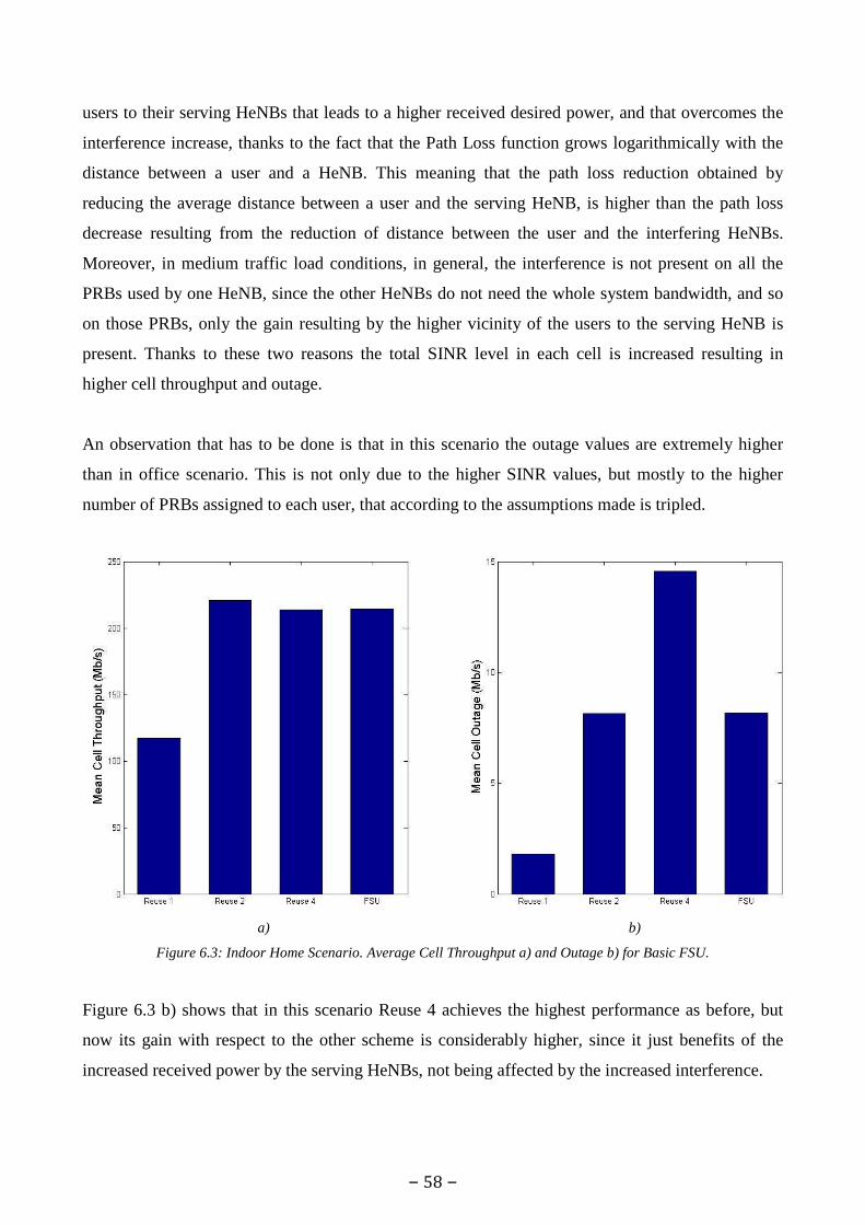
– 58 –

users to their serving HeNBs that leads to a higher received desired power, and that overcomes the

interference increase, thanks to the fact that the Path Loss function grows logarithmically with the

distance between a user and a HeNB. This meaning that the path loss reduction obtained by

reducing the average distance between a user and the serving HeNB, is higher than the path loss

decrease resulting from the reduction of distance between the user and the interfering HeNBs.

Moreover, in medium traffic load conditions, in general, the interference is not present on all the

PRBs used by one HeNB, since the other HeNBs do not need the whole system bandwidth, and so

on those PRBs, only the gain resulting by the higher vicinity of the users to the serving HeNB is

present. Thanks to these two reasons the total SINR level in each cell is increased resulting in

higher cell throughput and outage.

An observation that has to be done is that in this scenario the outage values are extremely higher

than in office scenario. This is not only due to the higher SINR values, but mostly to the higher

number of PRBs assigned to each user, that according to the assumptions made is tripled.

a) b)

Figure 6.3: Indoor Home Scenario. Average Cell Throughput a) and Outage b) for Basic FSU.

Figure 6.3 b) shows that in this scenario Reuse 4 achieves the highest performance as before, but

now its gain with respect to the other scheme is considerably higher, since it just benefits of the

increased received power by the serving HeNBs, not being affected by the increased interference.

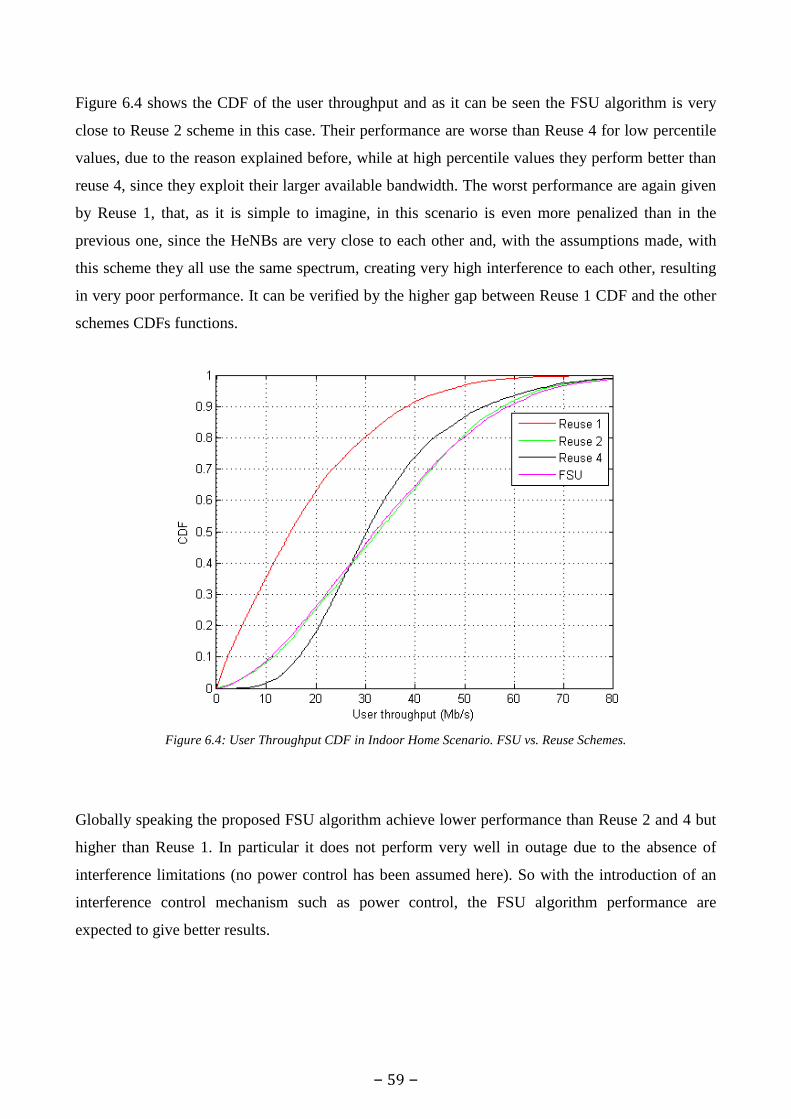
– 59 –

Figure 6.4 shows the CDF of the user throughput and as it can be seen the FSU algorithm is very

close to Reuse 2 scheme in this case. Their performance are worse than Reuse 4 for low percentile

values, due to the reason explained before, while at high percentile values they perform better than

reuse 4, since they exploit their larger available bandwidth. The worst performance are again given

by Reuse 1, that, as it is simple to imagine, in this scenario is even more penalized than in the

previous one, since the HeNBs are very close to each other and, with the assumptions made, with

this scheme they all use the same spectrum, creating very high interference to each other, resulting

in very poor performance. It can be verified by the higher gap between Reuse 1 CDF and the other

schemes CDFs functions.

Figure 6.4: User Throughput CDF in Indoor Home Scenario. FSU vs. Reuse Schemes.

Globally speaking the proposed FSU algorithm achieve lower performance than Reuse 2 and 4 but

higher than Reuse 1. In particular it does not perform very well in outage due to the absence of

interference limitations (no power control has been assumed here). So with the introduction of an

interference control mechanism such as power control, the FSU algorithm performance are

expected to give better results.

– 60 –

6.1.2 FSU with Power Control

Before starting to analyze the performance achieved by the use of power control, it is worth

verifying if the limitation introduced by power control effectively reduces the interference as it is

expected to do. In order to verify this, the interference on the Priority Chunks’ PRBs has been

evaluated for FSU with and without power control. The results are presented in figure 6.5, where

the mean interference level on the Priority Chunks’ PRBs for the two schemes and for 50 different

office scenarios is showed.

Figure 6.5: Priority Chunks’ PRBs Mean Interference Level in nW.

As it can be seen from the figure 6.5 the interference on the Priority Chunk’s PRBs is considerably

lower if power control is used, as it was supposed to be. In particular the average interference

reduction is in the order of 55%. Now that the first objective of power control has been verified, its

performance can be examined.

1) Static Indoor Office Scenario

Figure 6.6 a) and b) present the throughput and outage performance of the FSU algorithm with

power control compared to the other schemes analyzed before, for the indoor office scenario. From

figure 6.6 a) it can be seen that the throughput results increased with respect of the basic version of

the FSU algorithm, thanks to the interference reduction and the lower waste of spectrum. The value

– 61 –

of the gain is 10%. Despite this gain the FSU algorithm throughput is lower than Reuse 2 scheme

that is still the best scheme for throughput. Figure 6.6 b) instead shows that the introduction of

power control results in a considerable performance improvement in outage. In fact the gain

achieved by the use of power control is in the order of 80%. Moreover it performs even better than

Reuse 2 thanks to the extremely low interference, that is not totally absent as in Reuse 4, that still

achieves the highest outage throughput.

a) b)

Figure 6.6: Indoor Office Scenario. Average Cell Throughput a) and Outage b) for FSU with Power Control.

Considering the user throughput distribution, the CDF in figure 6.7 confirms that FSU with power

control has in general better performance than FSU without power control. In particular its gain is

more evident at percentiles lower than around the 70th. This is due to the high gain that users in bad

conditions experience thanks to the interference reduction achieved by power control, and this is

even more evident at very low percentiles up to the 20th, where the FSU with power control

performance are very close to reuse 4 scheme and slightly higher than reuse 2 scheme.

– 62 –

Figure 6.7: User Throughput CDF in Indoor Office Scenario. FSU with Power Control vs. Reuse Schemes.

2) Static Indoor Home Scenario

Figure 6.8 a) and b) present the results in indoor home scenario. The most relevant result given by

figure 6.8 is that in this scenario the FSU algorithm with power control achieves higher cell

throughput than Reuse 2 scheme, with a gain of 5%, reaching the highest performance between the

considered schemes. This is due to the fact that in the FSU algorithm the HeNBs can use as much

PRBs as needed, while the interference is maintained at a low level thanks to the presence of power

control and to the flexibility of the algorithm, that allows the HeNBs to choose always the PRBs on

which they experience the lowest interference. With respect to FSU without power control the gain

achieved in this scenario is 7.5% in throughput, 50% in outage.

In figure 6.9 the CDF of the user throughput is showed, and as it can be seen it confirms the

considerations resulting from figure 6.8. The FSU with power control has the best performance

apart that for values of percentile up to the 25th, where the Reuse 4 gives the highest performance.

– 63 –

a) b)

Figure 6.8: Indoor Home Scenario. Average Cell Throughput a) and Outage b) for FSU with Power Control.

Figure 6.9: User Throughput CDF in Indoor Home Scenario. FSU with Power Control vs. Reuse Schemes.

– 64 –

From the static simulations performed it can be derived that the proposed FSU algorithm, in

medium traffic load conditions, gives good performance, in particular in a very small range scenario

such as the indoor home scenario. Moreover the use of a mechanism, such as the power control, that

limits the interference created on the additional PRBs, brings a considerable gain, allowing our

algorithm to achieve performance comparable with the best fixed reuse schemes (Reuse 2 for the

cell throughput and Reuse 4 for the outage throughput). Moreover it has to be taken into account the

waste of power generated by the proposed FSU scheme, in order to perform the channel estimation,

that limits the achievable performance. The last but not the least thing that has always to be taken

into account, is that the FSU algorithm operates in self-optimizing manner without the necessity of

a previous preplanning while Reuse 2 and Reuse 4 schemes, which give respectively the best

throughput and outage performance between the reference schemes, require a preplanning phase.

Now that the proposed FSU algorithm has demonstrated to be able to achieve good performance, its

strength in a dynamic scenario has to be analyzed, in particular its self-configuration and, more

important, self-optimization capabilities in such scenarios.

6.2 Dynamic Simulations Results

Before starting to describe the results it is worth remembering that now, in the dynamic simulations,

both the PCFs are used, while in the static simulations only PCFocc is effectively used, due to the

absence of free chunks. So in this case both spectrum selection and power control are self-

optimized. We here remember that PCFocc and PCFfree are equal to 5% and 50% respectively.

6.2.1 FSU with Power Control vs. Reuse 2

1) Dynamic Indoor Office Scenario

Figure 6.10 shows the evolution of the cells throughput during the simulation execution. The time

index is reported on the x axis and the value of the throughput for each cell is reported on the y axis.

The vertical dotted lines represent the time index of entering and leaving events, used to clarify how

the performance change after one of these events.

– 65 –

Figure 6.10: Cells Throughput in Indoor Office Scenario. FSU with Power Control vs. Reuse 2.

From figure 6.10 it can be seen how the two compared schemes behave differently to entrance and

leaving events. The higher flexibility of the FSU algorithm can be clearly seen in the intervals

between two consecutive events, where the HeNBs try to adapt and optimize their configurations

after the last event. In particular two examples of the self-optimizing capability of the FSU

algorithm are marked by the two circles in the figure. From them it can be seen that after a

performance worsening due to a new HeNB entrance, the previous active HeNBs react changing

their spectrum selection, trying to overcome the potential performance decrease. In some cases they

are able to find other good (high SINR level) PRBs to use, bringing their performance at almost the

same level as they were before, as it happens in the cases marked by the two circles in figure 6.10,

but sometimes they cannot find so good PRBs and they can improve their performance just a little

bit. The latter case is more probable when there is an high number of active HeNBs, and so it is

difficult to find free or, in general, very good PRBs, as it can be clearly seen from figure 6.10, when

the HeNB-4 enters the system for the second time (time index=91) and, for example, HeNB-3 is not

able to bring its throughput at the same level it was before, because there are no more free (or with

very low interference) PRBs.

Moreover figure 6.10 shows that in the FSU algorithm an entrance or leaving event influences the

whole system, while in the Reuse 2 scheme at most one HeNB is influenced by one of those event.

In fact, after an entrance/leaving of an HeNB almost all the other HeNBs experience a throughput

decrease/increase in FSU, while in Reuse 2 only the HeNB to which the same spectrum is assigned,

– 66 –

i.e. HeNB in cell 3 (or 4) if the event happen in cell 1 (or 2) and vice versa. In figure 6.10 it can be

clearly seen in the interval between time index 76 (HeNB-4 leave the system) and 92 (HeNB-4

enter again in the system), where in FSU all the HeNBs experience a performance change, while in

Reuse 2, it happens only for one HeNB (HeNB-1 in this case). So the FSU has a higher fairness

between the HeNBs.

Even if in the FSU algorithm an entrance/leaving event causes reactions of all the active HeNBs,

the situation converges to a steady state after a short while, so the system is stable if no other

changes happen.

2) Dynamic Indoor Home Scenario

The self-optimization capabilities of the proposed FSU algorithm are even more evident looking at

figure 6.11. In particular it can be easily seen when the HeNB-4 (green line) enter for the second

time in the system (time index = 41), and the performance of HeNB-3 (pink line) considerably

decrease in Reuse 2, since the two HeNBs have the same usable spectrum. In the FSU algorithm,

instead, initially the throughput decrease, since HeNB-3 was using some PRBs belonging to the

fourth chunk, but as soon as it can update its spectrum, its performance rise up again, demonstrating

the FSU self-optimization. The same considerations made in the office scenario, about the HeNBs

fairness, can be done also in this scenario.

Figure 6.11: Cells Throughput in Indoor Home Scenario. FSU with Power Control vs. Reuse 2.

– 67 –

Globally speaking the proposed FSU algorithm achieves similar and, in some cases, even higher

performance than Reuse 2 confirming the results obtained in the static simulations. Further, in these

dynamic simulations its self-optimization capabilities have been demonstrated.

As it has been said before, the self-optimizing RRM capabilities we have considered are expressed

in terms of autonomous spectrum selection and the use of two different PCFs. The autonomous

spectrum selection has the greatest impact on the performance, since it aims at maximizing the

SINR level for each single HeNB reacting to changes in the system, while the use of two PCFs aims

to exploit the absence of some HeNBs. From the figures 6.10 and 6.11 the role and the impact of the

autonomous spectrum selection is clear, while the role and impact of the use of two PCFs instead

than only one have not been clarified yet by the previous simulations. Hence the FSU with the use

of two PCFs (PCFocc and PCFfree) has been compared also to a situation in which only PCFocc is

used on all the additional PRBs, regardless the respective chunk is occupied or not by any HeNB.

6.2.2 FSU with 2 PCFs vs. FSU with 1 PCF

In figure 6.12 and 6.13 it can be seen that the use of two different PCFs brings a throughput gain in

some circumstances, with respect to the case with only one PCF, for both indoor office and home

scenario. In particular the gain can be found when the HeNBs are not all active, since in that case

there is at least one free priority chunk and both of the PCFs are effectively used, while if all the

HeNBs are active only PCFocc is effectively used. In fact, as it can be seen for example from the

figures below (time index 56 – 76 and 91 – 111), the throughput of the two schemes are almost the

same when all the HeNBs are active. The gain is not present each time there are less than four

active HeNBs, since in some cases it can happen that the HeNB does not need additional spectrum

(NREQ < NPC), or that the gain resulting by the higher value of PCFfree is compensated by the higher

waste of power (in the case HeNB needs only a small number of additional PRBs), or by other

active HeNBs that are using the free chunk creating interference.

It can also be seen that when a HeNB changes its spectrum allocation, the performance variations,

with the use of two PCFs, are higher sometimes. This is due to the fact that the HeNB moves from a

PRB where it uses PCFocc to one where it can use PCFfree, or vice versa. This is what the use of two

PCFs was supposed to achieve, that is the exploitation of the presence of free Priority Chunks.

– 68 –

Figure 6.12: Cells Throughput in Indoor Office Scenario. FSU with 2 PCFs vs. FSU with 1 PCF.

Figure 6.13: Cells Throughput in Indoor Home Scenario. FSU with 2 PCFs vs. FSU with 1 PCF.

– 69 –

6.3 Dynamic Allocation Scheduling

6.3.1 Static Scenarios

In figure 6.14 and 6.15 the performance results for the static office and home scenarios are reported.

As it can be clearly seen from these pictures, and as it was expected to be, the use of a SINR aware

scheduling technique brings considerable improvements. Its performance are highly better in both

cell throughput and outage than all the other considered schemes that, we here remember, all use the

Round Robin scheduling. Referring to the FSU with Round Robin the throughput average gains

achieved are the 31% in office scenario and 20% in home scenario, while in the outage the gains are

85% and 42% respectively. The differences in gains for the two scenarios are due to the smaller

cells size of the home scenario. In fact, since the PRBs to use are selected by the HeNBs taking

those with the highest mean SINR level, it can happen that one or more PRBs are not good for some

users (for example those farther away from the base station), but they are particularly good for

someone else (those close to the base station), so the resulting mean SINR level is rather high and

they are selected as usable. In Round Robin, during the scheduling phase, these PRBs can be

allocated to the users for which they are bad PRBs, while in Dynamic Allocation it probably does

not happen since the HeNBs take into account the SINR level of each PRB for each user. In office

scenario the performance degradation due to the assignment of bad PRBs to users is higher than in

home scenario, since in the latter one even the users farther away from the base station cannot be

anyway too far. More clearly if we consider one PRB and two users, one placed in the best position

and one in the worst position for that PRB, the difference of the SINR levels of the two users in

home scenario will be surely smaller than in office scenario. Thus if that PRB will be assigned to

the user in worst condition instead that to the user in best condition, in home scenario the

performance worsening will be lower than in office scenario. So using a SINR aware PRB

scheduling such as Dynamic Allocation results in higher gain in office scenario.

Referring to the reuse schemes the use of the FSU with Dynamic Allocation achieves throughput

gains of 19% and 25% in office and home scenario respectively, with respect to Reuse 2 schemes

that resulted to be the best reuse scheme in cell throughput. Instead in outage throughput the best

reuse scheme is Reuse 4, against which the FSU with Dynamic Allocation achieves a gain of 45%

in office scenario and 29% in home scenario.

– 70 –

a) b)

Figure 6.14: FSU with Dynamic Allocation Scheduling Performance vs. Round Robin in Static Indoor Office Scenario.

a) b)

Figure 6.15: FSU with Dynamic Allocation Scheduling Performance vs. Round Robin in Static Indoor Home Scenario.

– 71 –

6.3.2 Dynamic Scenarios

Figures 6.16 and 6.17 report the results for dynamic indoor office and home scenarios respectively.

These results confirm what showed by the static simulations, i.e. that the use of Dynamic Allocation

brings significant improvement in cell throughput.

Anyway the aim of these simulations was principally to compare the reaction to changes of the two

schemes, and as it can be seen from the figures below, the reactions to changes in the system are

almost identical. This is due to the fact that the schedulers do not chose the spectrum to use by

themselves, but it is given to them as an input, and it is selected in the same way by each HeNB, as

specified in section 5.7. The schedulers are only responsible of allocating the given spectrum to the

users.

Figure 6.16: Cells Throughput in Dynamic Indoor Office Scenario. Dynamic Allocation Scheduling vs. Round Robin.

– 72 –

Figure 6.17: Cells Throughput in Dynamic Indoor Home Scenario. Dynamic Allocation Scheduling vs. Round Robin.

Finally, the Dynamic Allocation Scheduling has demonstrated to be an interesting addition to the

proposed FSU algorithm since it brings significant performance improvement, while maintaining

the same users fairness and the same reaction capabilities than Round Robin. Moreover it does not

require any additional information or particular operations, but just a modification in the way the

PRBs are assigned to users, so the added complexity is very low.

– 73 –

CHAPTER 7

Conclusions and Future Works

In this chapter the final considerations about the work of this thesis are given. In particular section

7.1 comments the obtained results and section 7.2 discusses the challenges related to future works.

7.1 Conclusions

This thesis deals with one of the most critical challenges that the expected large femtocells

deployment brings with it, that is the inter-cell interference management through the use of self-

optimization mechanisms. Self-optimized techniques are particularly useful in a scenario with

unpredictable and uncoordinated base stations deployment, as the Local Area Deployments are

supposed to be. In particular the proposed algorithm is focused on the automation of some Radio

Resource Management operations, such as spectrum selection and power control, always with the

final goal of minimizing the inter-cell interference while achieving high performance.

The self-optimization of the spectrum selection is performed through a Flexible Spectrum Usage

(FSU) mechanism, which allows the base stations to coexist and share a common spectrum pool in

a flexible manner. The coexistence and fairness between HeNBs is guaranteed by means of a

prioritization in the usage of parts of resource named Priority Chunks.

The static simulations showed that the proposed algorithm, that implements both FSU and power

control, achieves performance comparable with the best fixed reuse schemes for both mean cell

throughput and outage. In particular, in the smaller cell size scenario (home scenario) the proposed

algorithm’s achieved throughput is the best one, between the considered schemes. Moreover it has

to be considered that the FSU algorithm wastes a part of the total transmit power for the channel

estimation, reducing the achieved performance, while in the reuse schemes has been assumed that

the HeNBs always use the first NREQ PRBs between those available, without performing any

– 74 –

spectrum selection, so they do not need to transmit power for reference signals and the whole power

is used only for data transmission without wasting power.

The dynamic simulations demonstrated the proposed algorithm’s autonomous reaction capabilities,

which is a really interesting feature in such a scenario.

The main objective of the power control is to limit the interference, in particular on the HeNBs’

Priority Chunks. The interference reduction brings a considerable improvement in outage, i.e. the

throughput of the users in bad conditions. In particular the use of two power control factors allows a

self-optimized power allocation to PRBs, and is particularly beneficial when not all the resource

chunks are occupied.

A self-configuration mechanism is used, that is the Priority Chunk selection performed by the

HeNBs autonomously as soon as they are powered on, simply listening what the other potentially

active HeNBs are transmitting. So no pre-configuration and only a little amount of information

exchanged between the HeNBs are needed.

The last simulations have demonstrated how the performance of the proposed algorithm can be

easily improved by adding a bit of complexity to the scheduling phase, without the necessity of

additional information for the HeNBs.

Finally, the inter-cell interference management, flexible spectrum usage, self-configuration

(autonomous initial Priority Chunk selection) and self-optimization (autonomous spectrum selection

and double Power Control Factors usage) capabilities of the proposed algorithm, make it a valuable

solution for LTE-A Local Area Deployments.

7.2 Future Works

During the work of this thesis some simplifications have been made that could be reconsidered for

further studies. In particular the algorithm behavior in more realistic scenarios can be investigated.

– 75 –

Number of Priority Chunks

First of all, in order to allow the assignment of Priority Chunks to cells, it has been assumed that the

maximum number of cells in a scenario is known a priori (4 in our case). This assumption looks like

a sort of pre-planning, because the HeNBs should know that number that in general is different in

each specific scenario. One possible solution to this could be to find a scalable method to divide the

spectrum in chunks in a way that it adapts to the number of active HeNBs, e.g. if there are only two

active HeNBs, the whole spectrum is divided in two Priority Chunks, but when another HeNB

enters in the system another Priority Chunk is created taking an equal number of PRBs from the

previous two Priority Chunks. Another solution could be to fix a maximum number NMAX of Priority

Chunks that could be valid in whatever scenario, and if the actual number of active HeNBs is equal

to NMAX and another HeNB enters in the system, it can select the Priority Chunk selected by the

HeNB from which it experiences the lowest interference. Basically it is something similar to a reuse

scheme, where the selection of the Priority Chunk is performed autonomously. The value of NMAX

has to be accurately studied, since a too low value limits the scalability and can create too much

interference, since the HeNBs using the same Priority Chunk would be too close to each other.

Instead a too high value would limit the number of PRBs belonging to each Priority Chunk limiting

the performance as a consequence.

Traffic Model

Another simplification has been done on the traffic model. In this thesis it has been assumed that the

users requirement is expressed only in terms of number of PRBs, that is the same for all the users.

What happens in more realistic scenarios can be investigated, i.e. more realistic traffic models such

as Best Effort or Constant Bit Rate and different Quality of Service (QoS) requirement for each

user.

Dynamic Scenario

The dynamic scenario has been simulated only considering the entrance and leaving of base

stations. In the real world entrance or leaving events of the base stations are quite rare, while a

higher dynamism is expected for users that connect and disconnect more frequently to the network,

leading to variable traffic load conditions in the cells. Moreover no mobility has been assumed here,

while in the real world users use connection while they are on the move. How the proposed

algorithm behaves in such a scenario could be an interesting study subject.

– 76 –

Waste of Power

As explained in the simulations description, we have assumed that each HeNB that needs additional

spectrum transmits power on all the PRBs in order to allow the users to estimate the channel

condition. This causes a waste of power on the PRBs used only for channel estimation, that reduces

the useful power for data transmission, limiting the performance of the proposed algorithm. So if

the waste of power could be limited, the performance would be higher. A solution to this waste of

power could be to transmit the reference signal for channel estimation not on the whole band at all

the times, but alternatively on different parts of spectrum, for example only on one chunk at each

time interval. Thus at each time interval the power transmitted only for channel estimation is

reduced, limiting the waste of power. The disadvantage of this is less precise channel estimation,

since it is performed with lower frequency on each PRB, causing a slower reaction to changes in the

system. If a good trade-off between waste of power reduction and fast reaction to changes is found,

the performance of the proposed algorithm can be further improved. Moreover from a mobile

device point of view, performing the estimation on the whole bandwidth at each time is expensive

in terms of power consumption, therefore a mobile device would benefit from the reduction of the

band on which the estimation has to be done.

Scheduling Technique

Other possible studies can be done on the scheduling technique, considering the possibility of

adding self-optimization capabilities to it, meaning that it can be considered the possibility to adapt

the way the HeNBs allocate the PRBs to the users depending on the surrounding environment. For

example if the global interference level in a cell is particularly low, due for example to the absence

of surrounding active HeNBs, the HeNB could decide to adopt a scheduling that maximize the total

cell throughput, such as Max C/I (see section 2.1.5), reducing the fairness between users, since even

the penalized users will probably achieve good performance. The same solution can be used also if

the interference level is not so low, but if all the users in bad conditions do not have particular high

QoS requirements (e.g. require just a little amount of spectrum), so that the HeNB can prioritize

users in good condition without compromising the satisfaction of users in bad conditions. The

possibility to autonomously switch between different scheduling techniques depending on the users

requirement and surrounding environment, can surely bring significant performance improvements.

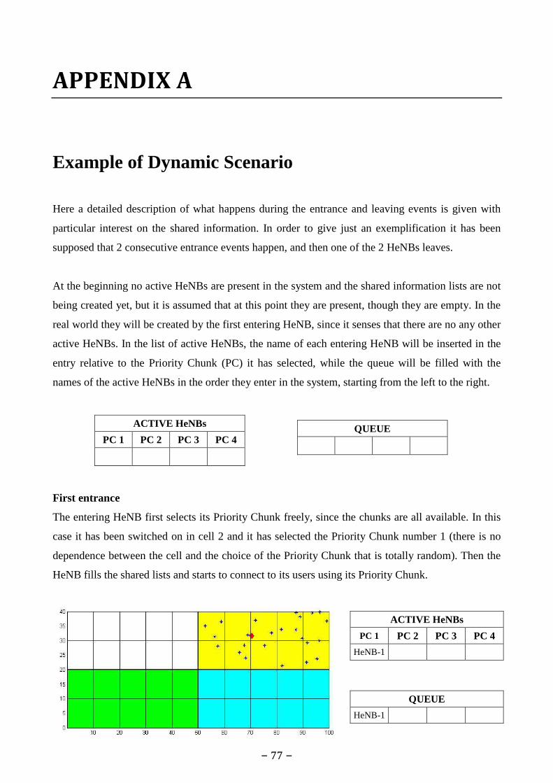
– 77 –

APPENDIX A

Example of Dynamic Scenario

Here a detailed description of what happens during the entrance and leaving events is given with

particular interest on the shared information. In order to give just an exemplification it has been

supposed that 2 consecutive entrance events happen, and then one of the 2 HeNBs leaves.

At the beginning no active HeNBs are present in the system and the shared information lists are not

being created yet, but it is assumed that at this point they are present, though they are empty. In the

real world they will be created by the first entering HeNB, since it senses that there are no any other

active HeNBs. In the list of active HeNBs, the name of each entering HeNB will be inserted in the

entry relative to the Priority Chunk (PC) it has selected, while the queue will be filled with the

names of the active HeNBs in the order they enter in the system, starting from the left to the right.

First entrance

The entering HeNB first selects its Priority Chunk freely, since the chunks are all available. In this

case it has been switched on in cell 2 and it has selected the Priority Chunk number 1 (there is no

dependence between the cell and the choice of the Priority Chunk that is totally random). Then the

HeNB fills the shared lists and starts to connect to its users using its Priority Chunk.

ACTIVE HeNBs

PC 1 PC 2 PC 3 PC 4

QUEUE

ACTIVE HeNBs

PC 1 PC 2 PC 3 PC 4

HeNB-1

QUEUE

HeNB-1

– 78 –

For clarity, the just entered HeNB has been called HeNB-1 not because it is the first to enter in the

system, but because it has chosen the Priority Chunk number 1, respecting the nomenclature used so

far in this thesis.

Subsequent entrances

When another HeNB enters the system and senses that an HeNB is already active, it reads the

shared lists received and selects one of the remaining Priority Chunks (2, 3 and 4 in this case)

autonomously. In this case the entering HeNB has selected the Priority Chunk number 4 and it has

been switched on in cell 1.

The queue is updated by adding HeNB-4 after HeNB-1, while the list of active HeNBs is updated

inserting the name of entering HeNB in the position relative to the Priority Chunk selected (4th in

this case). As soon as the HeNB-4 starts to transmit, HeNB-1 can update its knowledge about the

interference condition on all the PRBs.

Leaving event

When an HeNB leaves the system the only actions to do are to update the shared lists and the

interference knowledge by the other active HeNBs. If HeNB-1 leaves the system the shared

information are updated as follows:

ACTIVE HeNBs

PC 1 PC 2 PC 3 PC 4

HeNB-1 HeNB-4

QUEUE

HeNB-1 HeNB-4

QUEUE

HeNB-4

ACTIVE HeNBs

PC 1 PC 2 PC 3 PC4

HeNB-4

– 79 –

If later on, in cell 2 an HeNB will be switched on again, its position, the number and position of its

users and the Priority Chunk it will select will be completely uncorrelated with the previous

configuration.

Considering the nomenclature of the HeNBs used here, it can be noticed that the list of active

HeNBs can be even eliminated, since the queue already contains the information of which priority

chunks have been selected by the active HeNBs, and the list of active HeNBs does not give any

further information. Thus, in this case, the amount of information needed to be exchanged can be

reduced to the single queue information.

– 80 –

REFERENCES

[1] Cisco Visual Networking Index, “Global Mobile Data Traffic Forecast Update, 2009-2014”, Feb. 2010.

[2] UMTS forum, “Mobile Broadband Evolution: the roadmap from HSPA to LTE”, Feb. 2009.

[3] 3GPP TR 25.912, “Feasibility Study of Evolved UTRA and UTRA”, Sep. 2009.

[4] 3GPP TR 25.913, “Requirements for Evolved UTRA (E-UTRA) and Evolved UTRAN (E-UTRAN)”, Dec. 2009.

[5] Hyung G. Myung, “Technical Overview of 3GPP LTE”, May 2008.

[6] 3GPP TR 25.814, “Physical layer aspects for evolved Universal Terrestrial Radio Access (UTRA)”, Sep. 2006.

[7] R. Prasad, “OFDM for Wireless Communications Systems”. Artech House Publishers, 2003.

[8] 3GPP TR 25.892, version 6.0.0, “Feasibility study for OFDM for UTRAN Enhancement”, Jun. 2004.

[9] Ericsson White Paper, “LTE – An Introduction”, Jun. 2009.

[10] 3GPP TS 36.213, “Evolved Universal Terrestrial Radio Access (E-UTRA); Physical Layer Procedures”, Jun 2010.

[11] A.Pokhariyal, K.I. Pederson, G.Monghal, I.Z.Kovavs, C.Rosa, T.E. Kolding, P.E.Mogensen, “HARQ Aware Frequency Domain Packet Scheduler with Different Degrees of Fairness for the UTRAN Long Term Evolution”, Proc. IEEE Vehicular Technology Conference (VTC), Dublin, Apr. 2007, pp.2761-2765.

[12] G. Monghal, K.I. Pedersen, I.Z. Kovacs and P.E. Mogensen, “QoS Oriented Time and Frequency Domain Packet Schedulers for the UTRAN Long Term Evolution”, Proc. IEEE Vehicular Technology Conference (VTC), Singapore, May 2008.

[13] K. C. Beh, S. Armour, A. Doufexi, “Joint time-frequency domain proportional fair scheduler with HARQ for 3GPP LTE systems”, Proc. IEEE Vehicular Technology Conference (VTC), Calgary, Canada, Sept. 2008.

[14] Recommendation ITU-R M.1645, “Framework and overall objectives of the future development of IMT-2000 and systems beyond IMT-2000”.

[15] 3GPP TR 36.913, “Requirements for Further Advancements for E-UTRA (LTE-Advanced)”, May 2008.

– 81 –

[16] V. Chandrasekhar, J. G. Andrews, and A. Gatherer, “Femtocell Networks: A Survey”, IEEE Comm. Mag., Sept. 2008.

[17] 3G Americas, “The Benefits of SON in LTE”, Dec. 2009.

[18] 3GPP TS 32.500 “Telecommunication management; Self-Organizing Networks (SON); Concepts and requirements”, Dec. 2008.

[19] Sujuan Feng, Eiko Seidel, “Self-Organizing Networks (SON) in 3GPP Long Term Evolution”, Nomor Research, May 08.

[20] K. Hooli, et al., IST-2003-507581 WINNER, D6.3, “WINNER Spectrum Aspects: Assessment Report”, IST WINNER, Dec. 2005, http://www.istwinner.org.

[21] H. Claussen, L.T.W. Ho, and L.G. Samuel, “Financial Analysis of a Pico-Cellular Home Network Deployment”, IEEE ICC ’07, June 2007, pp. 5604–09.

[22] Y. Wang et al., "Fixed Frequency Reuse for LTE-Advanced Systems in Local Area Scenarios", Proc. IEEE Vehicular Technology Conference (VTC), Barcelona, Apr. 2009.

[23] IST-4-027756 WINNER II, D1.1.2 “WINNER II Channel Models part I- Channel Models”, Sep. 2007.

[24] Y. Wang, N. Marchetti et al., “An Interference Aware Dynamic Spectrum Sharing Algorithm for Local Area LTE-Advanced Networks”, Vehicular Technology Conference (VTC), Anchorage, AK, Sep. 2009.

[25] Sanjay Kumar, Y. Wang, N. Marchetti, I. Z. Kovacs and P. E. Mogensen, “Spectrum load Balancing for Flexible spectrum usage in Local area deployment Scenario”, IEEE symposium on Dynamic spectrum access 2008 (DySPAN 2008), Chicago, Oct. 2008.

[26] Sanjay Kumar, G. Monghal, Jaume Nin, Ivan Ordas, K. I. Pedersen, P. E. Mogensen, “Autonomous Inter Cell Interference Avoidance under Fractional Load for Downlink Long Term Evolution", Proc. IEEE Vehicular Technology Conference (VTC), Barcelona, 2009.

[27] R1-050764, Ericsson “Inter-cell Interference Handling for E-UTRA”, 3GPP TSG-RAN WG1 #42, London, Aug. 2005.

[28] R1-051051, LG Electronics, “Standard aspects for Interference coordination for EUTRA”, 3GPP TSG-RAN WG1 #42bis, San Diego, CA, Oct. 2005.

[29] R1-090236, Nokia Siemens Network, Nokia, “Inter eNB Over the Air Communication (OTAC) for LTE-Advanced”, 3GPP TSG RAN WG1 #55-bis, Ljubljana, Jan. 2009.