self labelling via simultaneous clustering ...much of the research in self-supervision has focused...
TRANSCRIPT

Published as a conference paper at ICLR 2020
SELF-LABELLING VIA SIMULTANEOUS CLUSTERINGAND REPRESENTATION LEARNING
Yuki M. Asano Christian Rupprecht Andrea Vedaldi
Visual Geometry GroupUniversity of Oxford{yuki,chrisr,vedaldi}@robots.ox.ac.uk
ABSTRACT
Combining clustering and representation learning is one of the most promisingapproaches for unsupervised learning of deep neural networks. However, doingso naively leads to ill posed learning problems with degenerate solutions. In thispaper, we propose a novel and principled learning formulation that addressesthese issues. The method is obtained by maximizing the information betweenlabels and input data indices. We show that this criterion extends standard cross-entropy minimization to an optimal transport problem, which we solve efficientlyfor millions of input images and thousands of labels using a fast variant of theSinkhorn-Knopp algorithm. The resulting method is able to self-label visual dataso as to train highly competitive image representations without manual labels. Ourmethod achieves state of the art representation learning performance for AlexNetand ResNet-50 on SVHN, CIFAR-10, CIFAR-100 and ImageNet and yields thefirst self-supervised AlexNet that outperforms the supervised Pascal VOC detectionbaseline. Code and models are available1.
1 INTRODUCTION
Learning from unlabelled data can dramatically reduce the cost of deploying machine learningalgorithms to new applications, thus amplifying their impact in the real world. Self-supervision is anincreasingly popular framework for learning without labels. The idea is to define pretext learningtasks that can be constructed from raw data alone, but that still result in neural networks that transferwell to useful applications.
Much of the research in self-supervision has focused on designing new pretext tasks. However,given supervised data such as ImageNet (Deng et al., 2009), the standard classification objective ofminimizing the cross-entropy loss still results in better or at least as good pre-training than any ofsuch methods (for a given amount of data and for a given model complexity). This suggests thatthe task of classification is sufficient for pre-training networks, provided that suitable data labelsare available. In this paper, we thus focus on the problem of obtaining the labels automatically bydesigning a self-labelling algorithm.
Learning a deep neural network together while discovering the data labels can be viewed as simultane-ous clustering and representation learning. The latter can be approached by combining cross-entropyminimization with an off-the-shelf clustering algorithm such as K-means. This is precisely theapproach adopted by the recent DeepCluster method (Caron et al., 2018), which achieves excellentresults in unsupervised representation learning. However, combining representation learning, whichis a discriminative task, with clustering is not at all trivial. In particular, we show that the combinationof cross-entropy minimization and K-means as adopted by DeepCluster cannot be described asthe optimization of an overall learning objective; instead, there exist degenerate solutions that thealgorithm avoids via particular implementation choices.
In order to address this technical shortcoming, in this paper, we contribute a new principled formula-tion for simultaneous clustering and representation learning. The starting point is to minimize a singleloss, the cross-entropy loss, for learning the deep network and for estimating the data labels. This
1https://github.com/yukimasano/self-label
1
arX
iv:1
911.
0537
1v3
[cs
.CV
] 1
9 Fe
b 20
20

Published as a conference paper at ICLR 2020
is often done in semi-supervised learning and multiple instance learning. However, when appliednaively to the unsupervised case, it immediately leads to a degenerate solution where all data pointsare mapped to the same cluster.
We solve this issue by adding the constraint that the labels must induce an equipartition of the data,which we show maximizes the information between data indices and labels. We also show that theresulting label assignment problem is the same as optimal transport, and can therefore be solved inpolynomial time by linear programming. However, since we want to scale the algorithm to millions ofdata points and thousands of labels, standard transport solvers are inadequate. Thus, we also proposeto use a fast version of the Sinkhorn-Knopp algorithm for finding an approximate solution to thetransport problem efficiently at scale, using fast matrix-vector algebra.
Compared to methods such as DeepCluster, the new formulation is more principled and allowsto more easily demonstrate properties of the method such as convergence. Most importantly, viaextensive experimentation, we show that our new approach leads to significantly superior resultsthan DeepCluster, achieving the new state of the art for representation learning approaches. Infact, the method’s performance surpasses others that use a single type of supervisory signal forself-supervision, and is on par or better than very recent contributions as well (Tian et al., 2019; Heet al., 2019; Misra & van der Maaten, 2019; Oord et al., 2018).
2 RELATED WORK
Our paper relates to two broad areas of research: (a) self-supervised representation learning, and (b)more specifically, training a deep neural network using pseudo-labels, i.e. the assignment of a labelto each image. We discuss closely related works for each.
Self-supervised learning: A wide variety of methods that do not require manual annotations havebeen proposed for the self-training of deep convolutional neural networks. These methods usevarious cues and proxy tasks namely, in-painting (Pathak et al., 2016), patch context and jigsawpuzzles (Doersch et al., 2015; Noroozi & Favaro, 2016; Noroozi et al., 2018; Mundhenk et al.,2017), clustering (Caron et al., 2018; Huang et al., 2019; Zhuang et al., 2019; Bautista et al., 2016),noise-as-targets (Bojanowski & Joulin, 2017), colorization (Zhang et al., 2016; Larsson et al., 2017),generation (Jenni & Favaro, 2018; Ren & Lee, 2018; Donahue et al., 2017; Donahue & Simonyan,2019), geometry (Dosovitskiy et al., 2016), predicting transformations (Gidaris et al., 2018; Zhanget al., 2019) and counting (Noroozi et al., 2017). Most recently, contrastive methods have showngreat performance gains, (Oord et al., 2018; Hénaff et al., 2019; Tian et al., 2019; He et al., 2019)by leveraging augmentation and adequate losses. In (Feng et al., 2019), predicting rotation (Gidariset al., 2018) is combined with instance retrieval (Wu et al., 2018) and multiple tasks are combined in(Doersch & Zisserman, 2017).
Pseudo-labels for images: In the self-supervised domain, we find a spectrum of methods that eithergive each data point a unique label (Wu et al., 2018; Dosovitskiy et al., 2016) or train on a flexiblenumber of labels with K-means (Caron et al., 2018), with mutual information (Ji et al., 2018) or withnoise (Bojanowski & Joulin, 2017). In (Noroozi et al., 2018) a large network is trained with a pretexttask and a smaller network is trained via knowledge transfer of the clustered data. Finally, (Bach &Harchaoui, 2008; Vo et al., 2019) use convex relaxations to regularized affine-transformation invariantlinear clustering, but can not scale to larger datasets.
Our contribution is a simple method that combines a novel pseudo-label extraction procedure fromraw data alone and the training of a deep neural network using a standard cross-entropy loss.
3 METHOD
We will first derive our self-labelling method, then interpret the method as optimizing labels andtargets of a cross-entropy loss and finally analyze similarities and differences with other clustering-based methods.
3.1 SELF-LABELLING
Neural network pre-training is often achieved via a supervised data classification task. Formally,consider a deep neural network x = Φ(I) mapping data I (e.g. images) to feature vectors x ∈ RD.The model is trained using a dataset (e.g. ImageNet) of N data points I1, . . . , IN with corresponding
2

Published as a conference paper at ICLR 2020
labels y1, . . . , yN ∈ {1, . . . ,K}, drawn from a space of K possible labels. The representation isfollowed by a classification head h : RD → RK , usually consisting of a single linear layer, convertingthe feature vector into a vector of class scores. The class scores are mapped to class probabilities viathe softmax operator:
p(y = ·|xi) = softmax(h ◦ Φ(xi)).
The model and head parameters are learned by minimizing the average cross-entropy loss
E(p|y1, . . . , yN ) = − 1
N
N∑i=1
log p(yi|xi). (1)
Training with objective (1) requires a labelled dataset. When labels are unavailable, we require aself-labelling mechanism to assign the labels automatically.
In semi-supervised learning, self-labelling is often achieved by jointly optimizing (1) with respectto the model h ◦ Φ and the labels y1, . . . , yN . This can work if at least part of the labels are known,thus constraining the optimization. However, in the fully unsupervised case, it leads to a degeneratesolution: eq. (1) is trivially minimized by assigning all data points to a single (arbitrary) label.
To address this issue, we first rewrite eq. (1) by encoding the labels as posterior distributions q(y|xi):
E(p, q) = − 1
N
N∑i=1
K∑y=1
q(y|xi) log p(y|xi). (2)
If we set the posterior distributions q(y|xi) = δ(y−yi) to be deterministic, the formulations in eqs. (1)and (2) are equivalent, in the sense that E(p, q) = E(p|y1, . . . , yN ). In this case, optimizing q is thesame as reassigning the labels, which leads to the degeneracy. To avoid this, we add the constraintthat the label assignments must partition the data in equally-sized subsets. Formally, the learningobjective objective2 is thus:
minp,q
E(p, q) subject to ∀y : q(y|xi) ∈ {0, 1} andN∑i=1
q(y|xi) =N
K. (3)
The constraints mean that each data point xi is assigned to exactly one label and that, overall, the Ndata points are split uniformly among the K classes.
The objective in eq. (3) is combinatorial in q and thus may appear very difficult to optimize. However,this is an instance of the optimal transport problem, which can be solved relatively efficiently. In orderto see this more clearly, let Pyi = p(y|xi) 1
N be the K ×N matrix of joint probabilities estimated bythe model. Likewise, let Qyi = q(y|xi) 1
N be K ×N matrix of assigned joint probabilities. Usingthe notation of (Cuturi, 2013), we relax matrix Q to be an element of the transportation polytope
U(r, c) := {Q ∈ RK×N+ | Q1 = r, Q>1 = c}. (4)
Here 1 are vectors of all ones of the appropriate dimensions, so that r and c are the marginalprojections of matrix Q onto its rows and columns, respectively. In our case, we require Q to be amatrix of conditional probability distributions that split the data uniformly, which is captured by:
r =1
K· 1, c =
1
N· 1.
With this notation, we can rewrite the objective function in eq. (3), up to a constant shift, as
E(p, q) + logN = 〈Q,− logP 〉, (5)
where 〈·〉 is the Frobenius dot-product between two matrices and log is applied element-wise. Henceoptimizing eq. (3) with respect to the assignments Q is equivalent to solving the problem:
minQ∈U(r,c)
〈Q,− logP 〉. (6)
2We assume for simplicity that K divides N exactly, but the formulation is easily extended to any N ≥ Kby setting the constraints to either bN/Kc or bN/Kc+ 1, in order to assure that there is a feasible solution.
3

Published as a conference paper at ICLR 2020
This is a linear program, and can thus be solved in polynomial time. Furthermore, solving thisproblem always leads to an integral solution despite having relaxed Q to the continuous polytopeU(r, c), guaranteeing the exact equivalence to the original problem.
In practice, however, the resulting linear program is large, involving millions of data points andthousands of classes. Traditional algorithms to solve the transport problem scale badly to instancesof this size. We address this issue by adopting a fast version (Cuturi, 2013) of the Sinkhorn-Knoppalgorithm. This amounts to introducing a regularization term
minQ∈U(r,c)
〈Q,− logP 〉+1
λKL(Q‖rc>), (7)
where KL is the Kullback-Leibler divergence and rc> can be interpreted as a K ×N probabilitymatrix. The advantage of this regularization term is that the minimizer of eq. (7) can be written as:
Q = diag(α)Pλ diag(β) (8)
where exponentiation is meant element-wise and α and β are two vectors of scaling coefficientschosen so that the resulting matrix Q is also a probability matrix (see (Cuturi, 2013) for a derivation).The vectors α and β can be obtained, as shown below, via a simple matrix scaling iteration.
For very large λ, optimizing eq. (7) is of course equivalent to optimizing eq. (6), but even formoderate values of λ the two objectives tend to have approximately the same optimizer (Cuturi,2013). Choosing λ trades off convergence speed with closeness to the original transport problem.In our case, using a fixed λ is appropriate as we are ultimately interested in the final clustering andrepresentation learning results, rather than in solving the transport problem exactly.
Our final algorithm’s core can be described as follows. We learn a model h◦Φ and a label assignmentmatrix Q by solving the optimization problem eq. (6) with respect to both Q, which is a probabilitymatrix, and the model h ◦ Φ, which determines the predictions Pyi = softmaxy(h ◦ Φ(xi)). We doso by alternating the following two steps:
Step 1: representation learning. Given the current label assignments Q, the model is updated byminimizing eq. (6) with respect to (the parameters of) h ◦ Φ. This is the same as training the modelusing the common cross-entropy loss for classification.
Step 2: self-labelling. Given the current model h ◦ Φ, we compute the log probabilities P . Then,we find Q using eq. (8) by iterating the updates (Cuturi, 2013)
∀y : αy ← [Pλβ]−1y ∀i : βi ← [α>Pλ]−1i .
Each update involves a single matrix-vector multiplication with complexityO(NK), so it is relativelyquick even for millions of data points and thousands of labels and so the cost of this method scaleslinearly with the number of images N . In practice, convergence is reached within 2 minutes onImageNet when computed on a GPU. Also, note that the parameters α and β can be retained betweensteps, thus allowing a warm start of Step 2.
3.2 INTERPRETATION
As shown above, the formulation in eq. (2) uses scaled versions of the probabilities. We can interpretthese by treating the data index i as a random variable with uniform distribution p(i) = 1/N andby rewriting the posteriors p(y|xi) = p(y|i) and q(y|xi) = q(y|i) as conditional distributions withrespect to the data index i instead of the feature vector xi. With these changes, we can rewrite eq. (5)as
E(p, q) + logN = −N∑i=1
K∑y=1
q(y, i) log p(y, i) = H(q, p), (9)
which is the cross-entropy between the joint label-index distributions q(y, i) and p(y, i). The mini-mum of this quantity w.r.t. q is obtained when p = q, in which case E(q, q) + logN reduces to theentropy Hq(y, i) of the random variables y and i. Additionally, since we assumed that q(i) = 1/N ,the marginal entropy Hq(i) = logN is constant and, due to the equipartition condition q(y) = 1/K,Hq(y) = logK is also constant. Subtracting these two constants from the entropy yields:
minpE(p, q)+logN = E(q, q)+logN = Hq(y, i) = Hq(y)+Hq(i)−Iq(y, i) = const.−Iq(y, i).
4

Published as a conference paper at ICLR 2020
Thus we see that minimizing E(p, q) is the same as maximizing the mutual information between thelabel y and the data index i.
In our formulation, the maximization above is carried out under the equipartition constraint. We caninstead relax this constraint and directly maximize the information I(y, i). However, by rewritinginformation as the difference I(y, i) = H(y)−H(y|i), we see that the optimal solution is given byH(y|i) = 0, which states each data point i is associated to only one label deterministically, and byH(y) = lnK, which is another way of stating the equipartition condition.
In other words, our learning formulation can be interpreted as maximizing the information betweendata indices and labels while explicitly enforcing the equipartition condition, which is implied bymaximizing the information in any case. Compared to minimizing the entropy alone, maximizinginformation avoids degenerate solutions as the latter carry no mutual information between labels yand indices i. Similar considerations can be found in (Ji et al., 2018).
3.3 RELATION TO SIMULTANEOUS REPRESENTATION LEARNING AND CLUSTERING
In the discussion above, self-labelling amounts to assigning discrete labels to data and can thus beinterpreted as clustering. Most of the traditional clustering approaches are generative. For example,K-means takes a dataset x1, . . . ,xN of vectors and partitions it into K classes in order to minimizethe reconstruction error
E(µ1, . . . ,µK , y1, . . . , yN ) =1
N
N∑i=1
‖xi − µyi‖2 (10)
where yi ∈ {1, . . . ,K} are the data-to-cluster assignments and µy are means approximating thevectors in the corresponding clusters. The K-means energy can thus be interpreted as the averagedata reconstruction error.
It is natural to ask whether a clustering method such as K-means, which is based on approximatingthe input data, could be combined with representation learning, which uses a discriminative objective.In this setting, the feature vectors x = Φ(I) are extracted by the neural network Φ from the input dataI . Unfortunately, optimizing a loss such as eq. (10) with respect to the clustering and representationparameters is meaningless: in fact, the obvious solution is to let the representation send all the datapoints to the same constant feature vector and setting all the means to coincide with it, in which casethe K-means reconstruction error is zero (and thus minimal).
Nevertheless, DeepCluster (Caron et al., 2018) does successfully combine K-means with represen-tation learning. DeepCluster can be related to our approach as follows. Step 1 of the algorithm,namely representation learning via cross-entropy minimization, is exactly the same. Step 2, namelyself-labelling, differs: where we solve an optimal transport problem to obtain the pseudo-labels, theydo so by running K-means on the feature vectors extracted by the neural network.
DeepCluster does have an obvious degenerate solution: we can assign all data points to the samelabel and learn a constant representation, achieving simultaneously a minimum of the cross-entropyloss in Step 1 and of the K-means loss in Step 2. The reason why DeepCluster avoids this pitfall isdue to the particular interaction between the two steps. First, during Step 2, the features xi are fixedso K-means cannot pull them together. Instead, the means spread to cover the features as they are,resulting in a balanced partitioning. Second, during the classification step, the cluster assignments yiare fixed, and optimizing the features xi with respect to the cross-entropy loss tends to separate them.Lastly, the method in (Caron et al., 2018) also uses other heuristics such as sampling the training datainversely to their associated clusters’ size, leading to further regularization.
However, a downside of DeepCluster is that it does not have a single, well-defined objective tooptimize, which means that it is difficult to characterize its convergence properties. By contrast, in ourformulation, both Step 1 and Step 2 optimize the same objective, with the advantage that convergenceto a (local) optimum is guaranteed.
3.4 AUGMENTING SELF-LABELLING VIA DATA TRANSFORMATIONS
Methods such as DeepCluster extend the training data via augmentations. In vision problems, thisamounts to (heavily) distorting and cropping the input images at random. Augmentations are appliedso that the neural network is encouraged to learn a labelling function which is transformation invariant.
5

Published as a conference paper at ICLR 2020
In practice, this is crucial to learn good clusters and representations, so we adopt it here. This isachieved by setting Pyi = Et[log softmaxy h ◦ Φ(txi)] where the transformations t are sampled atrandom. In practice, in Step 1 (representation learning), this is implemented via the application of therandom transformations to data batches during optimization via SGD, which is corresponds to theusual data augmentation scheme for deep neural networks. As noted in (YM. et al., 2020), and as canbe noted by an analysis of recent publications (Hénaff et al., 2019; Tian et al., 2019; Misra & van derMaaten, 2019), augmentation is critical for good performance.
3.5 MULTIPLE SIMULTANEOUS SELF-LABELINGS
Intuitively, the same data can often be clustered in many equally good ways. For example, visualobjects can be clustered by color, size, typology, viewpoint, and many other attributes. Since ourmain objective is to use clustering to learn a good data representation Φ, we consider a multi-tasksetting in which the same representation is shared among several different clustering tasks, which canpotentially capture different and complementary clustering axis.
In our formulation, this is easily achieved by considering multiple heads (Ji et al., 2018) h1, . . . , hT ,one for each of T clustering tasks (which may also have a different number of labels). Then, weoptimize a sum of objective functions of the type eq. (6), one for each task, while sharing theparameters of the feature extractor Φ among them.
4 EXPERIMENTS
In this section, we evaluate the quality of the representations learned by our Self Labelling (SeLa)technique. We first test variants of our method, including ablating its components, in order to findan optimal configuration. Then, we compare our results to the state of the art in self-supervisedrepresentation learning, where we find that our method is the best among clustering-based techniquesand overall state-of-the-art or at least highly competitive in many benchmarks. In the appendix, wealso show qualitatively that the labels identified by our algorithm are usually meaningful and groupvisually similar concepts in the same clusters, often even capturing whole ImageNet classes.
4.1 SETUP
Linear probes. In order to quantify if a neural network has learned useful feature representations,we follow the standard approach of using linear probes (Zhang et al., 2017). This amounts to solvinga difficult task, such as ImageNet classification, by training a linear classifier on top of a pre-trainedfeature representation, which is kept fixed. Linear classifiers heavily rely on the quality of therepresentation since their discriminative power is low. We apply linear probes to all intermediateconvolutional blocks of representative networks. While linear probes are conceptually straightforward,there are several technical details that can affect the final accuracy, so we follow the standard protocolfurther outlined in the Appendix.
Data. For training data we consider ImageNet LSVRC-12 (Deng et al., 2009) and other smallerscale datasets. We also test our features by transferring them to MIT Places (Zhou et al., 2014). Allof these are standard benchmarks for evaluation in self-supervised learning.
Architectures. Our base encoder architecture is AlexNet (Krizhevsky et al., 2012), since this is themost frequently used in other self-supervised learning works for the purpose of benchmarking. Weinject the probes right after the ReLU layer in each of the five blocks, and denote these entry pointsconv1 to conv5. Furthermore, since the conv1 and conv2 can be learned effectively from dataaugmentations alone (YM. et al., 2020), we focus the analysis on the deeper layers conv2 to conv5which are more sensitive to the quality of the learning algorithm. In addition to AlexNet, we also testResNet-50 (He et al., 2016) models. Further experimental details are given in the Appendix.
4.2 OPTIMAL CONFIGURATION AND ABLATIONS
In tables 1 and 5, we first validate various modelling and configuration choices. Two key hyper-parameters are the number of clusters K and the number of clustering heads T , which we denote inthe experiments below with the shorthand “SeLa[K × T ]”. We run SeLa by alternating steps 1 and 2as described in section 3.1. Step 1 amounts to standard CE training, which we run for a fixed numberof epochs. Step 2 can be interleaved at any point in the optimization; to amortize its cost, we run it
6

Published as a conference paper at ICLR 2020
Table 1: Ablation: number ofself-labelling steps.Method #opt. c3 c4 c5
SeLa [3k× 1] 0 20.8 18.3 13.4SeLa [3k× 1] 40 42.7 43.4 39.2SeLa [3k× 1] 80 43.0 44.7 40.9SeLa [3k× 1] 160 42.4 44.6 40.7
Table 2: Number of clustersK.
Method c3 c4 c5
SeLa [1k× 1] 40.1 42.1 38.8SeLa [3k× 1] 43.0 44.7 40.9SeLa [5k× 1] 42.5 43.9 40.2SeLa [10k× 1] 42.2 43.8 39.7
Table 3: Ablation: number ofheads T . (c4 for AlexNet)Method Architecture Top-1
SeLa [3k× 1] AlexNet 44.7SeLa [3k× 10] AlexNet 46.7
SeLa [3k× 1] ResNet-50 51.8SeLa [3k× 10] ResNet-50 61.5
Table 4: Different architectures.Method Architecture Top-1
SeLa [3k× 1] AlexNet (small) 41.3SeLa [3k× 1] AlexNet 44.7SeLa [3k× 1] ResNet-50 51.8
Table 5: Label transfer.Method Source (Top-1) Target (Top-1)
SeLa [3k× 10] AlexNet (46.7) AlexNet (46.5)
SeLa [3k× 1] ResNet-50 (51.8) AlexNet (45.0)SeLa [3k× 10] ResNet-50 (61.5) AlexNet (48.4)
at most once per epoch, and usually less, with a schedule described and validated below. For theseexperiments, we train the representation and the linear probes on ImageNet.
Number of clusters K. Table 2, compares different values for K: moving from 1k to 3k improvesthe results, but larger numbers decrease the quality slightly.
Ablation: number of heads T . Table 3 shows that increasing the number of heads from T = 1 toT = 10 yields a large performance gain: +2% for AlexNet and +10% for ResNet. The latter moreexpressive model appears to benefit more from a more diverse training signal.
Ablation: number of self-labelling iterations. First, in table 1, we show that self-labelling (step 2)is essential for good performance, as opposed to only relying on the initial random label assignmentsand the data augmentations. For this, we vary the number of times the self-labelling algorithm (step2) is run during training (#opts), from zero to once per step 1 epoch. We see that self-labelling isessential, with the best value around 80 (for 160 step 1 epochs in total).
Architectures. Table 4 compares a smaller variant of AlexNet which uses (64, 192) filters in itsfirst two convolutional layers (Krizhevsky, 2014), to the standard variant with (96, 256) (Krizhevskyet al., 2012), all the way to a ResNet-50. SeLa works well in all cases, for large models such asResNet but also smaller ones such as AlexNet, for which methods such as BigBiGAN (Donahue &Simonyan, 2019) or CPC (Hénaff et al., 2019) are unsuitable.
4.3 LABEL TRANSFER
An appealing property of SeLa is that the label it assigns to the images can be used to train anothermodel from scratch, using standard supervised training. For instance, table 5 shows that, given thelabels assigned by applying SeLa to AlexNet, we can re-train AlexNet from scratch using a shorter90-epochs schedule with achieving the same final accuracy. This shows that the quality of the learnedrepresentation depends only the final label assignment, not on the fact that the representation is learnedjointly with the labels. More interestingly, we can transfer labels between different architectures. Forexample, the labels obtained by applying SeLa [3k× 1] and SeLa [3k× 10] to ResNet-50 can be usedto train a better AlexNet model than applying SeLa to the latter directly. For this reason, we publishon our website the self-labels for the ImageNet dataset in addition to the code and trained models.
4.4 SMALL-SCALE DATASETS
Here, we evaluate our method on relatively simple and small datasets, namelyCIFAR-10/100 (Krizhevsky et al., 2009) and SVHN (Netzer et al., 2011). For this, we fol-low the experimental and evaluation protocol from the current state of the art in self-supervisedlearning in these datasets, AND (Huang et al., 2019). In table 6, we compare our method with thesettings [128 × 10] for CIFAR-10, [512 × 10] for CIFAR-100 and [128 × 1] for SVHN to otherpublished methods; details on the evaluation method are provided in the appendix. We observe thatour proposed method outperforms the best previous method by 5.8% for CIFAR-10, by 9.5% forCIFAR-100 and by 0.8% for SVHN when training a linear classifier on top of the frozen network.The relatively minor gains on SVHN can be explained by the fact that the gap between the supervised
7

Published as a conference paper at ICLR 2020
Table 6: Nearest Neighbour and linear classificationevaluation on small datasets using AlexNet. Resultsof previous methods are taken from (Huang et al.,2019).
DatasetMethod CIFAR-10 CIFAR-100 SVHN
Classifier/Feature Linear Classifier / conv5Supervised 91.8 71.0 96.1Counting 50.9 18.2 63.4DeepCluster 77.9 41.9 92.0Instance 70.1 39.4 89.3AND 77.6 47.9 93.7
SL 83.4 57.4 94.5
Classifier/Feature Weighted kNN / FCSupervised 91.9 69.7 96.5Counting 41.7 15.9 43.4DeepCluster 62.3 22.7 84.9Instance 60.3 32.7 79.8AND 74.8 41.5 90.9
SL 77.6 44.2 92.8
Table 7: PASCAL VOC finetun-ing. VOC07-Classification %mAP,VOC07-Detection %mAP and VOC12-Segmentation %mIU. ∗ denotes a largerAlexNet variant.
PASCAL VOC TaskMethod Cls. Det. Seg.
fc6-8 all all all
ImageNet labels 78.9 79.9 59.1 48.0Random − 53.3 43.4 −Random Rescaled − 56.6 45.6 32.6
BiGAN 52.3 60.1 46.9 35.2Context∗ 55.1 65.3 51.1 −Context 2 − 69.6 55.8 41.4CC+VGG − 72.5 56.5 42.6RotNet 70.9 73.0 54.4 39.1DeepCluster∗ 72.0 73.4 55.4 45.1RotNet+retrieval∗ 72.5 74.7 58.0 45.9
SeLa∗ [3k× 10] 73.1 75.3 55.9 43.7SeLa∗ [3k× 10]− 74.4 75.9 57.8 44.7SeLa∗ [3k× 10]−+Rot 75.6 77.2 59.2 45.7
Table 8: Nearest Neighbour and linear classification evaluation using imbalanced CIFAR-10 trainingdata. We evaluate on the normal CIFAR-10 test set and on CIFAR-100 to analyze the transferabilityof the features. Difference to the supervised baseline in parentheses. See section 4.5 for details.
kNN Linear/conv5
Training data/Method CIFAR-10 CIFAR-100 CIFAR-10 CIFAR-100
CIFAR-10, fullSupervised 92.1 24.0 90.2 54.2ours (K-means) [128× 1] 64.7 (−17.4) 19.3 (−4.7) 77.5 (−12.7) 45.6 (−8.8)ours (SK) [128× 1] 72.9 (−9.2) 28.9 (+4.9) 79.8 (−9.4) 49.4 (−4.8)
CIFAR-10, light imbalanceSupervised 92.0 24.0 90.4 53.6ours (K-means) [128× 1] 64.2 (−17.8) 18.1 (−5.9) 77.0 (−13.4) 44.8 (−8.8)ours (SK) [128× 1] 71.7 (−10.3) 28.2 (+4.2) 79.5 (−10.9) 48.6 (−5.0)
CIFAR-10, heavy imbalanceSupervised 86.7 22.6 86.8 51.4ours (K-means) [128× 1] 60.7 (−16.0) 17.8 (−4.8) 75.2 (−11.6) 44.3 (−7.1)ours (SK) [128× 1] 67.6 (−9.1) 26.7 (+3.9) 77.2 (−9.6) 47.5 (−2.9)
baseline and the self-supervised results is already very small (<3%). We also evaluate our methodusing weighted kNN using an embedding of size 128. We find that the proposed method consistentlyoutperforms the previous state of the art by around 2% across these datasets, even though AND isbased on explicitly learning local neighbourhoods.
4.5 IMBALANCED DATA EXPERIMENTS
In order to understand if our equipartition regularization is affected by the underlying class distributionof a dataset, we perform multiple ablation experiments on artificially imbalanced datasets in table 8.We consider three training datasets based on CIFAR-10. The first is the original dataset with 5000images for each class (full in table 8). Second, we remove 50% of the images of one class (truck) whilethe rest remains untouched (light imbalance) and finally we remove 10% of one class, 20% of thesecond class and so on (heavy imbalance). On each of the three datasets we compare the performanceof our method “ours (SK)” with a baseline that replaces our Sinkhorn-Knopp optimization withK-means clustering “ours (K-means)”. We also compare the performance to training a networkunder full supervision. The evaluation follows Huang et al. (2019) and is based on linear probing andkNN classification — both on CIFAR-10 and, to understand feature generalization, on CIFAR-100.
8
Published as a conference paper at ICLR 2020
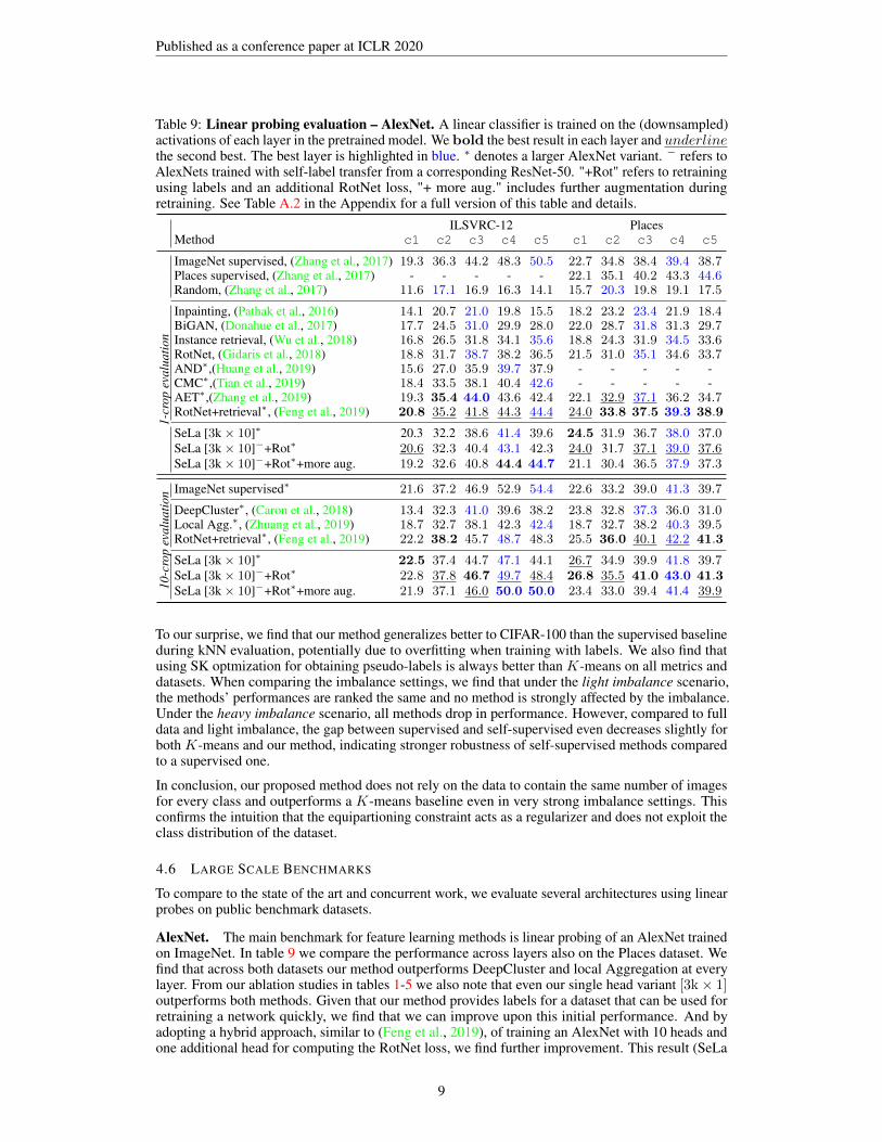
Table 9: Linear probing evaluation – AlexNet. A linear classifier is trained on the (downsampled)activations of each layer in the pretrained model. We bold the best result in each layer and underlinethe second best. The best layer is highlighted in blue. ∗ denotes a larger AlexNet variant. − refers toAlexNets trained with self-label transfer from a corresponding ResNet-50. "+Rot" refers to retrainingusing labels and an additional RotNet loss, "+ more aug." includes further augmentation duringretraining. See Table A.2 in the Appendix for a full version of this table and details.
ILSVRC-12 PlacesMethod c1 c2 c3 c4 c5 c1 c2 c3 c4 c5
ImageNet supervised, (Zhang et al., 2017) 19.3 36.3 44.2 48.3 50.5 22.7 34.8 38.4 39.4 38.7Places supervised, (Zhang et al., 2017) - - - - - 22.1 35.1 40.2 43.3 44.6Random, (Zhang et al., 2017) 11.6 17.1 16.9 16.3 14.1 15.7 20.3 19.8 19.1 17.5
Inpainting, (Pathak et al., 2016) 14.1 20.7 21.0 19.8 15.5 18.2 23.2 23.4 21.9 18.4BiGAN, (Donahue et al., 2017) 17.7 24.5 31.0 29.9 28.0 22.0 28.7 31.8 31.3 29.7
1-cr
opev
alua
tion Instance retrieval, (Wu et al., 2018) 16.8 26.5 31.8 34.1 35.6 18.8 24.3 31.9 34.5 33.6
RotNet, (Gidaris et al., 2018) 18.8 31.7 38.7 38.2 36.5 21.5 31.0 35.1 34.6 33.7AND∗,(Huang et al., 2019) 15.6 27.0 35.9 39.7 37.9 - - - - -CMC∗,(Tian et al., 2019) 18.4 33.5 38.1 40.4 42.6 - - - - -AET∗,(Zhang et al., 2019) 19.3 35.4 44.0 43.6 42.4 22.1 32.9 37.1 36.2 34.7RotNet+retrieval∗, (Feng et al., 2019) 20.8 35.2 41.8 44.3 44.4 24.0 33.8 37.5 39.3 38.9
SeLa [3k× 10]∗ 20.3 32.2 38.6 41.4 39.6 24.5 31.9 36.7 38.0 37.0SeLa [3k× 10]−+Rot∗ 20.6 32.3 40.4 43.1 42.3 24.0 31.7 37.1 39.0 37.6SeLa [3k× 10]−+Rot∗+more aug. 19.2 32.6 40.8 44.4 44.7 21.1 30.4 36.5 37.9 37.3
10-c
rop
eval
uatio
n ImageNet supervised∗ 21.6 37.2 46.9 52.9 54.4 22.6 33.2 39.0 41.3 39.7
DeepCluster∗, (Caron et al., 2018) 13.4 32.3 41.0 39.6 38.2 23.8 32.8 37.3 36.0 31.0Local Agg.∗, (Zhuang et al., 2019) 18.7 32.7 38.1 42.3 42.4 18.7 32.7 38.2 40.3 39.5RotNet+retrieval∗, (Feng et al., 2019) 22.2 38.2 45.7 48.7 48.3 25.5 36.0 40.1 42.2 41.3
SeLa [3k× 10]∗ 22.5 37.4 44.7 47.1 44.1 26.7 34.9 39.9 41.8 39.7SeLa [3k× 10]−+Rot∗ 22.8 37.8 46.7 49.7 48.4 26.8 35.5 41.0 43.0 41.3SeLa [3k× 10]−+Rot∗+more aug. 21.9 37.1 46.0 50.0 50.0 23.4 33.0 39.4 41.4 39.9
To our surprise, we find that our method generalizes better to CIFAR-100 than the supervised baselineduring kNN evaluation, potentially due to overfitting when training with labels. We also find thatusing SK optmization for obtaining pseudo-labels is always better than K-means on all metrics anddatasets. When comparing the imbalance settings, we find that under the light imbalance scenario,the methods’ performances are ranked the same and no method is strongly affected by the imbalance.Under the heavy imbalance scenario, all methods drop in performance. However, compared to fulldata and light imbalance, the gap between supervised and self-supervised even decreases slightly forboth K-means and our method, indicating stronger robustness of self-supervised methods comparedto a supervised one.
In conclusion, our proposed method does not rely on the data to contain the same number of imagesfor every class and outperforms a K-means baseline even in very strong imbalance settings. Thisconfirms the intuition that the equipartioning constraint acts as a regularizer and does not exploit theclass distribution of the dataset.
4.6 LARGE SCALE BENCHMARKS
To compare to the state of the art and concurrent work, we evaluate several architectures using linearprobes on public benchmark datasets.
AlexNet. The main benchmark for feature learning methods is linear probing of an AlexNet trainedon ImageNet. In table 9 we compare the performance across layers also on the Places dataset. Wefind that across both datasets our method outperforms DeepCluster and local Aggregation at everylayer. From our ablation studies in tables 1-5 we also note that even our single head variant [3k× 1]outperforms both methods. Given that our method provides labels for a dataset that can be used forretraining a network quickly, we find that we can improve upon this initial performance. And byadopting a hybrid approach, similar to (Feng et al., 2019), of training an AlexNet with 10 heads andone additional head for computing the RotNet loss, we find further improvement. This result (SeLa
9

Published as a conference paper at ICLR 2020
Table 10: Linear evaluation - ResNet. A linear layer is trained on top of the global average pooledfeatures of ResNets. All evaluations use a single centred crop. We have separated much largerarchitectures such as RevNet-50×4 and ResNet-161. Methods in brackets use a augmentationpolicy learned from supervised training and methods with ∗ are not explicit about which furtheraugmentations they use. See Table A.3 in the Appendix for a full version of this table.
Method Architecture Top-1 Top-5
Supervised, (Donahue & Simonyan, 2019) ResNet-50 76.3 93.1
Jigsaw, (Kolesnikov et al., 2019) ResNet-50 38.4 −Rotation, (Kolesnikov et al., 2019) ResNet-50 43.8 −CPC, (Oord et al., 2018) ResNet-101 48.7 73.6BigBiGAN, (Donahue & Simonyan, 2019) ResNet-50 55.4 77.4LocalAggregation, (Zhuang et al., 2019) ResNet-50 60.2 −Efficient CPC v2.1, (Hénaff et al., 2019) ResNet-50 (63.8) (85.3)CMC, (Tian et al., 2019) ResNet-50 (64.1) (85.4)MoCo, (He et al., 2019) ResNet-50 60.6 −PIRL, (Misra & van der Maaten, 2019)∗ ResNet-50 63.6 −SeLa [3k× 10] ResNet-50 61.5 84.0
other architecturesMoCo, (He et al., 2019) RevNet-50×4 68.6 −Efficient CPC v2.1, (Hénaff et al., 2019) ResNet-161 71.5 90.1
[3k× 10]−+Rot) achieves state of the art in unsupervised representation learning for AlexNet, witha gap of 1.3% to the previous best performance on ImageNet and surpasses the ImageNet supervisedbaseline transferred to Places by 1.7%.
ResNet. Training better models than AlexNets is not yet standardized in the feature learningcommunity. In Table 10 we compare a ResNet-50 trained with our method to other works. With top-1accuracy of 61.5, we outperform than all other methods including Local Aggregation, CPCv1 andMoCo that use the same level of data augmentation. We even outperform larger architectures such asBigBiGAN’s RevNet-50x4 and reach close to the performance of models using AutoAugment-styletransformations.
4.7 FINE-TUNING: CLASSIFICATION, OBJECT DETECTION AND SEMANTIC SEGMENTATION
Finally, since pre-training is usually aimed at improving down-stream tasks, we evaluate the quality ofthe learned features by fine-tuning the model for three distinct tasks on the PASCAL VOC benchmark.In Table 7 we compare results with regard to multi-label classification, object detection and semanticsegmentation on PASCAL VOC (Everingham et al., 2010).
As in the linear probe experiments, we find our method better than the current state of the art indetection and classification with both fine-tuning only the last fully connected layers and whenfine-tuning the whole network (“all”. Notably, our fine-tuned AlexNet outperforms its supervisedImageNet baseline on the VOC detection task. Also for segmentation the method is very close (0.2%)to the best performing method. This shows that our trained network does not only learn useful featurerepresentations but is also able to perform well when fine-tuned on actual down-stream tasks.
5 CONCLUSION
We present a self-supervised feature learning method that is based on clustering. In contrast to othermethods, ours optimizes the same objective during feature learning and during clustering. Thisbecomes possible through a weak assumption that the number of samples should be equal acrossclusters. This constraint is explicitly encoded in the label assignment step and can be solved forefficiently using a modified Sinkhorn-Knopp algorithm. Our method outperforms all other featurelearning approaches and achieves SOTA on SVHN, CIFAR-10/100 and ImageNet for AlexNet andResNet-50. By virtue of the method, the resulting self-labels can be used to quickly learn features fornew architectures using simple cross-entropy training.
10
Published as a conference paper at ICLR 2020
ACKNOWLEDGMENTS
Yuki Asano gratefully acknowledges support from the EPSRC Centre for Doctoral Training inAutonomous Intelligent Machines & Systems (EP/L015897/1). We are also grateful to ERC IDIU-638009, AWS Machine Learning Research Awards (MLRA) and the use of the University of OxfordAdvanced Research Computing (ARC).
REFERENCES
Francis R. Bach and Zaïd Harchaoui. Diffrac: a discriminative and flexible framework for clustering.In J. C. Platt, D. Koller, Y. Singer, and S. T. Roweis (eds.), Advances in Neural InformationProcessing Systems 20, pp. 49–56. Curran Associates, Inc., 2008. 2
Philip Bachman, R Devon Hjelm, and William Buchwalter. Learning representations by maximizingmutual information across views. arXiv preprint arXiv:1906.00910, 2019. 18
Miguel A Bautista, Artsiom Sanakoyeu, Ekaterina Tikhoncheva, and Björn Ommer. Cliquecnn:Deep unsupervised exemplar learning. In Proceedings of the Conference on Advances in NeuralInformation Processing Systems (NIPS), pp. 3846–3854, 2016. 2
Piotr Bojanowski and Armand Joulin. Unsupervised learning by predicting noise. In Proc. ICML, pp.517–526. PMLR, 2017. 2
M. Caron, P. Bojanowski, A. Joulin, and M. Douze. Deep clustering for unsupervised learning ofvisual features. In Proc. ECCV, 2018. 1, 2, 5, 9, 14, 15, 16, 17
Marco Cuturi. Sinkhorn distances: Lightspeed computation of optimal transport. In Advances inneural information processing systems, pp. 2292–2300, 2013. 3, 4, 14
J. Deng, W. Dong, R. Socher, L.-J. Li, K. Li, and L. Fei-Fei. Imagenet: A large-scale hierarchicalimage database. In Proc. CVPR, 2009. 1, 6
Carl Doersch and Andrew Zisserman. Multi-task self-supervised visual learning. In Proc. ICCV,2017. 2, 18
Carl Doersch, Abhinav Gupta, and Alexei A Efros. Unsupervised visual representation learning bycontext prediction. In Proc. ICCV, pp. 1422–1430, 2015. 2, 17
Jeff Donahue and Karen Simonyan. Large scale adversarial representation learning, 2019. 2, 7, 10,18
Jeff Donahue, Philipp Krähenbühl, and Trevor Darrell. Adversarial feature learning. Proc. ICLR,2017. 2, 9, 17
A. Dosovitskiy, P. Fischer, J. T. Springenberg, M. Riedmiller, and T. Brox. Discriminative unsuper-vised feature learning with exemplar convolutional neural networks. IEEE PAMI, 38(9):1734–1747,Sept 2016. ISSN 0162-8828. doi: 10.1109/TPAMI.2015.2496141. 2
Mark Everingham, Luc Van Gool, Christopher KI Williams, John Winn, and Andrew Zisserman.The pascal visual object classes (voc) challenge. International journal of computer vision, 88(2):303–338, 2010. 10
Zeyu Feng, Chang Xu, and Dacheng Tao. Self-supervised representation learning by rotation featuredecoupling. In Proceedings of the IEEE Conference on Computer Vision and Pattern Recognition,pp. 10364–10374, 2019. 2, 9, 17
Spyros Gidaris, Praveen Singh, and Nikos Komodakis. Unsupervised representation learning bypredicting image rotations. In Proc. ICLR, 2018. 2, 9, 17
Kaiming He, Xiangyu Zhang, Shaoqing Ren, and Jian Sun. Identity mappings in deep residualnetworks. In European conference on computer vision, pp. 630–645. Springer, 2016. 6
Kaiming He, Haoqi Fan, Yuxin Wu, Saining Xie, and Ross Girshick. Momentum contrast forunsupervised visual representation learning, 2019. 2, 10, 18
11

Published as a conference paper at ICLR 2020
Olivier J Hénaff, Ali Razavi, Carl Doersch, SM Eslami, and Aaron van den Oord. Data-efficientimage recognition with contrastive predictive coding. arXiv preprint arXiv:1905.09272v2, 2019. 2,6, 7, 10, 18
Jiabo Huang, Q Dong, Shaogang Gong, and Xiatian Zhu. Unsupervised deep learning by neighbour-hood discovery. In Proceedings of the International Conference on machine learning (ICML),2019. 2, 7, 8, 9, 14, 17
Simon Jenni and Paolo Favaro. Self-supervised feature learning by learning to spot artifacts. In Proc.CVPR, 2018. 2, 17
Xu Ji, João F Henriques, and Andrea Vedaldi. Invariant information distillation for unsupervisedimage segmentation and clustering. arXiv preprint arXiv:1807.06653, 2018. 2, 5, 6
Alexander Kolesnikov, Xiaohua Zhai, and Lucas Beyer. Revisiting self-supervised visual representa-tion learning. arXiv preprint arXiv:1901.09005, 2019. 10, 18
A. Krizhevsky, I. Sutskever, and G. E. Hinton. ImageNet classification with deep convolutional neuralnetworks. In NIPS, pp. 1106–1114, 2012. 6, 7
Alex Krizhevsky. One weird trick for parallelizing convolutional neural networks. arXiv preprintarXiv:1404.5997, 2014. 7
Alex Krizhevsky et al. Learning multiple layers of features from tiny images. Technical report,Citeseer, 2009. 7
Gustav Larsson, Michael Maire, and Gregory Shakhnarovich. Colorization as a proxy task for visualunderstanding. In Proc. CVPR, 2017. 2
Ishan Misra and Laurens van der Maaten. Self-supervised learning of pretext-invariant representations,2019. 2, 6, 10, 18
T Mundhenk, Daniel Ho, and Barry Y. Chen. Improvements to context based self-supervised learning.In Proc. CVPR, 2017. 2
T. Nathan Mundhenk, Daniel Ho, and Barry Y. Chen. Improvements to context based self-supervisedlearning. pp. 9339–9348, 2018. 17
Yuval Netzer, Tao Wang, Adam Coates, Alessandro Bissacco, Bo Wu, and Andrew Ng. Readingdigits in natural images with unsupervised feature learning. NIPS, 01 2011. 7
Mehdi Noroozi and Paolo Favaro. Unsupervised learning of visual representations by solving jigsawpuzzles. In Proc. ECCV, pp. 69–84. Springer, 2016. 2, 17
Mehdi Noroozi, Hamed Pirsiavash, and Paolo Favaro. Representation learning by learning to count.In Proc. ICCV, 2017. 2, 17
Mehdi Noroozi, Ananth Vinjimoor, Paolo Favaro, and Hamed Pirsiavash. Boosting self-supervisedlearning via knowledge transfer. In Proc. CVPR, 2018. 2, 17
Aaron van den Oord, Yazhe Li, and Oriol Vinyals. Representation learning with contrastive predictivecoding. arXiv preprint arXiv:1807.03748, 2018. 2, 10, 18
Deepak Pathak, Philipp Krahenbuhl, Jeff Donahue, Trevor Darrell, and Alexei A Efros. Contextencoders: Feature learning by inpainting. In Proc. CVPR, pp. 2536–2544, 2016. 2, 9, 17
Zhongzheng Ren and Yong Jae Lee. Cross-domain self-supervised multi-task feature learning usingsynthetic imagery. In Proc. CVPR, 2018. 2
Yonglong Tian, Dilip Krishnan, and Phillip Isola. Contrastive multiview coding, 2019. 2, 6, 9, 10, 17,18
Nguyen Xuan Vinh, Julien Epps, and James Bailey. Information theoretic measures for clusteringscomparison: Variants, properties, normalization and correction for chance. Journal of MachineLearning Research, 11(Oct):2837–2854, 2010. 14
12
Published as a conference paper at ICLR 2020
Huy V Vo, Francis Bach, Minsu Cho, Kai Han, Yann LeCun, Patrick Pérez, and Jean Ponce.Unsupervised image matching and object discovery as optimization. In Proceedings of the IEEEConference on Computer Vision and Pattern Recognition, pp. 8287–8296, 2019. 2
Zhirong Wu, Yuanjun Xiong, Stella X Yu, and Dahua Lin. Unsupervised feature learning via non-parametric instance discrimination. In Proceedings of the IEEE Conference on Computer Visionand Pattern Recognition, pp. 3733–3742, 2018. 2, 9, 14, 17
Asano YM., Rupprecht C., and Vedaldi A. A critical analysis of self-supervision, or what we canlearn from a single image. In International Conference on Learning Representations, 2020. URLhttps://openreview.net/forum?id=B1esx6EYvr. 6
Liheng Zhang, Guo-Jun Qi, Liqiang Wang, and Jiebo Luo. Aet vs. aed: Unsupervised representationlearning by auto-encoding transformations rather than data. In Proceedings of the IEEE Conferenceon Computer Vision and Pattern Recognition, pp. 2547–2555, 2019. 2, 9, 17
Richard Zhang, Phillip Isola, and Alexei A Efros. Colorful image colorization. In Proc. ECCV, pp.649–666. Springer, 2016. 2, 17
Richard Zhang, Phillip Isola, and Alexei A. Efros. Split-brain autoencoders: Unsupervised learningby cross-channel prediction. In Proc. CVPR, 2017. 6, 9, 14, 17
Bolei Zhou, Agata Lapedriza, Jianxiong Xiao, Antonio Torralba, and Aude Oliva. Learning deepfeatures for scene recognition using places database. In Advances in neural information processingsystems, pp. 487–495, 2014. 6
Chengxu Zhuang, Alex Lin Zhai, and Daniel Yamins. Local aggregation for unsupervised learning ofvisual embeddings. In Proceedings of the IEEE International Conference on Computer Vision, pp.6002–6012, 2019. 2, 9, 10, 17, 18
13

Published as a conference paper at ICLR 2020
A APPENDIX
A.1 IMPLEMENTATION DETAILS
Learning Details Unless otherwise noted, we train all our self-supervised models with SGD andintial learning rate 0.05 for 400 epochs with two learning rate drops where we divide the rateby ten at 150 and 300 and 350 epochs. We spread our pseudo-label optimizations throughoutthe whole training process in a logarithmic distribution. We optimize the label assignment at
ti =(
iM−1
)2, i ∈ {1, . . . ,M}, where M is the user-defined number of optimizations and ti is
expressed as a fraction of total training epochs. For the Sinkhorn-Knopp optimization we set λ = 25as in (Cuturi, 2013). We use standard data augmentations during training that consist of randomlyresized crops, horizontal flipping and adding noise, as in (Wu et al., 2018).
Quantitative Evaluation – Technical Details. Unfortunately, prior work has used several slightlydifferent setups, so that comparing results between different publications must be done with caution.
In our ImageNet implementation, we follow the original proposal (Zhang et al., 2017) in poolingeach representation to a vector with 9600, 9216, 9600, 9600, 9216 dimensions for conv1-5 usingadaptive max-pooling, and absorb the batch normalization weights into the preceding convolutions.For evaluation on ImageNet we follow RotNet to train linear probes: images are resized such thatthe shorter edge has a length of 256 pixels, random crops of 224×224 are computed and flippedhorizontally with 50% probability. Learning lasts for 36 epochs and the learning rate schedulestarts from 0.01 and is divided by five at epochs 5, 15 and 25. The top-1 accuracy of the linearclassifier is then measured on the ImageNet validation subset by optionally extracting 10 crops foreach validation image (four at the corners and one at the center along with their horizontal flips)and averaging the prediction scores before the accuracy is computed or just taking the a centredcrop. For CIFAR-10/100 and SVHN we train AlexNet architectures on the resized images withbatchsize 128, learning rate 0.03 and also the same image augmentations (random resized crops,color jitter and random grayscale) as is used in prior work (Huang et al., 2019). We use the samelinear probing protocol as for our ImageNet experiments but without using 10 crops. For the weightedkNN experiments we use k = 50, σ = 0.1 and we use an embedding of size 128 as done in previousworks.
In Table 9, when retraining an AlexNet using ResNet generated labels, we can apply heavieraugmentation strategies as the labels are kept constant. Hence for the experiments denoted by "+more aug.", in addition to the usual augmentations, we further randomly apply one of equalize,autoconstrast and sharpening. We find that this raises the performance for ImageNet but lowersthe performance on Places by a small amount, hence illuminating the need to always also reportperformance on both datasets.
A.2 FURTHER DETAILS
NMI over time In fig. A.1 we find that most learning takes place in the early epochs, and we reacha final NMI value of around 66%. Similarly, we find that due to the updating of the pseudo-labels atregular intervals and our data augmentation, the pseudo-label accuracies keep continuously risingwithout overfitting to these labels.
Clustering metrics In table A.1, we report standard clustering metrics (see (Vinh et al., 2010)for detailed definitions) of our trained models with regards to the ImageNet validation set ground-truth labels. These metrics include chance-corrected metrics which are the adjusted normalizedmutual information (NMI) and the adjusted Rand-Index, as well as the default NMI, also reported inDeepCluster (Caron et al., 2018).
Conv1 filters In fig. A.3 we show the first convolutional filters of two of our trained models. Wecan find the typical Gabor-like edge detectors as well as color blops and dot-detectors.
Entropy over time In fig. A.4, we show how the distribution of entropy with regards to the trueImageNet labels changes with training time. We find that while at first, all 3000 pseudo-labels containrandom real ImageNet labels, yielding high entropy of around 6 ≈ ln(400) = ln(1.2 · 106/3000).Towards the end of training we arrive at a broad spectrum of entropies with some as low as
14

Published as a conference paper at ICLR 2020
0 100 200 300 400epochs
0.5
0.6
0.7
0.8
0.9
NMI t
-1 /
t
Figure A.1: Left: Normalized Mutual Information (NMI) against validation set ImageNet labels.This measure is not used for training but indicates how good a clustering is. Right: Similarities ofconsecutive labellings using NMI. Both plots use the [10k× 1] AlexNet for comparability with theDeepCluster paper (Caron et al., 2018).
Table A.1: Clustering metrics that compare with ground-truth labels of the ImageNet validation set(with 1-crop). For reference, we provide the best Top-1 error on ImageNet linear probing (as reportedin the main part).∗: for the multi-head variants, we simply use predictions of a randomly picked,single head.
Metricsadjusted
Variant NMI adjusted NMI Rand-Index Top-1 Acc.
SeLa [1k× 1] AlexNet 50.5% 12.2% 2.7% 42.1%SeLa [3k× 1] AlexNet 59.1% 9.8% 2.5% 44.7%SeLa [5k× 1] AlexNet 66.2% 7.4% 1.8% 43.9%SeLa [10k× 1] AlexNet 66.4% 4.7% 1.0% 43.8%SeLa [3k× 1] ResNet-50 60.0% 13.5% 3.8% 51.8%SeLa [3k× 10]∗ ResNet-50 66.3% 26.4% 10.3% 61.5%
Figure A.2: Pseudo-label accuracies for the training data versus training time for the [10k × 1]AlexNet.
Figure A.3: Visualization of the first convolutional layers of our [3k × 10] AlexNet (left) and the[1k× 1] ResNet-50 (right). The filters are scaled to lie between (0,1) for visualization.
0.07 ≈ ln(1.07) (see Fig. A.5 and A.6 for low entropy label visualizations) and the mean around4.2 ≈ ln(66) (see Fig. A.7 and A.8 for randomly chosen labels’ visualizations).
15

Published as a conference paper at ICLR 2020
0123456Entropy
0.0
0.5
1.0
1.5
2.0
2.5
3.0startduringafter training
Figure A.4: Cross-entropy of the pseudo-labels with the true ImageNet training set labels. Thismeasure is not used for training but indicates how good a clustering is. This plot uses the [10k× 1]AlexNet to compare to the equivalent plot in (Caron et al., 2018).
A.3 COMPLETE TABLES
In the following, we report the unabridged tables with all related work.
16
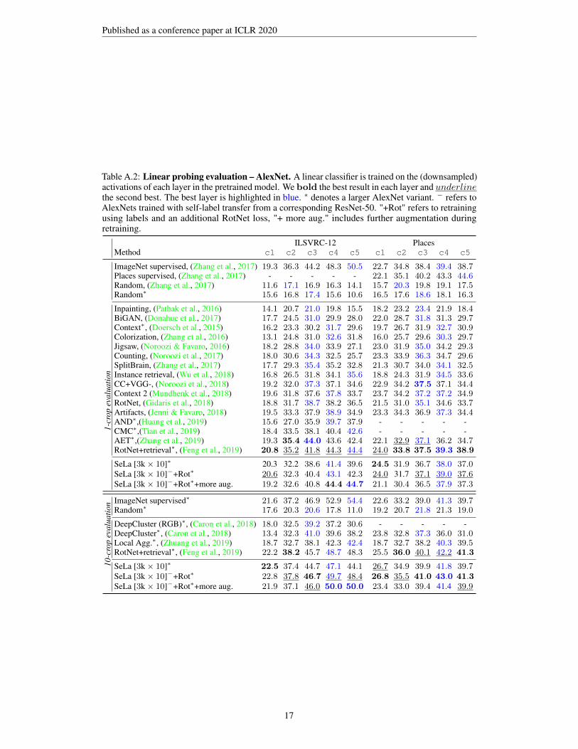
Published as a conference paper at ICLR 2020
Table A.2: Linear probing evaluation – AlexNet. A linear classifier is trained on the (downsampled)activations of each layer in the pretrained model. We bold the best result in each layer and underlinethe second best. The best layer is highlighted in blue. ∗ denotes a larger AlexNet variant. − refers toAlexNets trained with self-label transfer from a corresponding ResNet-50. "+Rot" refers to retrainingusing labels and an additional RotNet loss, "+ more aug." includes further augmentation duringretraining.
ILSVRC-12 PlacesMethod c1 c2 c3 c4 c5 c1 c2 c3 c4 c5
ImageNet supervised, (Zhang et al., 2017) 19.3 36.3 44.2 48.3 50.5 22.7 34.8 38.4 39.4 38.7Places supervised, (Zhang et al., 2017) - - - - - 22.1 35.1 40.2 43.3 44.6Random, (Zhang et al., 2017) 11.6 17.1 16.9 16.3 14.1 15.7 20.3 19.8 19.1 17.5Random∗ 15.6 16.8 17.4 15.6 10.6 16.5 17.6 18.6 18.1 16.3
Inpainting, (Pathak et al., 2016) 14.1 20.7 21.0 19.8 15.5 18.2 23.2 23.4 21.9 18.4BiGAN, (Donahue et al., 2017) 17.7 24.5 31.0 29.9 28.0 22.0 28.7 31.8 31.3 29.7Context∗, (Doersch et al., 2015) 16.2 23.3 30.2 31.7 29.6 19.7 26.7 31.9 32.7 30.9Colorization, (Zhang et al., 2016) 13.1 24.8 31.0 32.6 31.8 16.0 25.7 29.6 30.3 29.7Jigsaw, (Noroozi & Favaro, 2016) 18.2 28.8 34.0 33.9 27.1 23.0 31.9 35.0 34.2 29.3Counting, (Noroozi et al., 2017) 18.0 30.6 34.3 32.5 25.7 23.3 33.9 36.3 34.7 29.6SplitBrain, (Zhang et al., 2017) 17.7 29.3 35.4 35.2 32.8 21.3 30.7 34.0 34.1 32.5
1-cr
opev
alua
tion Instance retrieval, (Wu et al., 2018) 16.8 26.5 31.8 34.1 35.6 18.8 24.3 31.9 34.5 33.6
CC+VGG-, (Noroozi et al., 2018) 19.2 32.0 37.3 37.1 34.6 22.9 34.2 37.5 37.1 34.4Context 2 (Mundhenk et al., 2018) 19.6 31.8 37.6 37.8 33.7 23.7 34.2 37.2 37.2 34.9RotNet, (Gidaris et al., 2018) 18.8 31.7 38.7 38.2 36.5 21.5 31.0 35.1 34.6 33.7Artifacts, (Jenni & Favaro, 2018) 19.5 33.3 37.9 38.9 34.9 23.3 34.3 36.9 37.3 34.4AND∗,(Huang et al., 2019) 15.6 27.0 35.9 39.7 37.9 - - - - -CMC∗,(Tian et al., 2019) 18.4 33.5 38.1 40.4 42.6 - - - - -AET∗,(Zhang et al., 2019) 19.3 35.4 44.0 43.6 42.4 22.1 32.9 37.1 36.2 34.7RotNet+retrieval∗, (Feng et al., 2019) 20.8 35.2 41.8 44.3 44.4 24.0 33.8 37.5 39.3 38.9
SeLa [3k× 10]∗ 20.3 32.2 38.6 41.4 39.6 24.5 31.9 36.7 38.0 37.0SeLa [3k× 10]−+Rot∗ 20.6 32.3 40.4 43.1 42.3 24.0 31.7 37.1 39.0 37.6SeLa [3k× 10]−+Rot∗+more aug. 19.2 32.6 40.8 44.4 44.7 21.1 30.4 36.5 37.9 37.3
10-c
rop
eval
uatio
n ImageNet supervised∗ 21.6 37.2 46.9 52.9 54.4 22.6 33.2 39.0 41.3 39.7Random∗ 17.6 20.3 20.6 17.8 11.0 19.2 20.7 21.8 21.3 19.0
DeepCluster (RGB)∗, (Caron et al., 2018) 18.0 32.5 39.2 37.2 30.6 - - - - -DeepCluster∗, (Caron et al., 2018) 13.4 32.3 41.0 39.6 38.2 23.8 32.8 37.3 36.0 31.0Local Agg.∗, (Zhuang et al., 2019) 18.7 32.7 38.1 42.3 42.4 18.7 32.7 38.2 40.3 39.5RotNet+retrieval∗, (Feng et al., 2019) 22.2 38.2 45.7 48.7 48.3 25.5 36.0 40.1 42.2 41.3
SeLa [3k× 10]∗ 22.5 37.4 44.7 47.1 44.1 26.7 34.9 39.9 41.8 39.7SeLa [3k× 10]−+Rot∗ 22.8 37.8 46.7 49.7 48.4 26.8 35.5 41.0 43.0 41.3SeLa [3k× 10]−+Rot∗+more aug. 21.9 37.1 46.0 50.0 50.0 23.4 33.0 39.4 41.4 39.9
17

Published as a conference paper at ICLR 2020
Table A.3: Linear evaluation - ResNet. A linear layer is trained on top of the global averagepooled features of ResNets. All evaluations use a single centred crop. We have separated muchlarger architectures such as RevNet-50×4 and ResNet-161. Methods in brackets use a augmentationpolicy learned from supervised training and methods with ∗ are not explicit about which furtheraugmentations they use.
Method Architecture Top-1 Top-5
Supervised, (Donahue & Simonyan, 2019) ResNet-50 76.3 93.1Supervised, (Donahue & Simonyan, 2019) ResNet-101 77.8 93.8
Jigsaw, (Kolesnikov et al., 2019) ResNet-50 38.4 −RelPathLoc, (Kolesnikov et al., 2019) ResNet-50 42.2 −Exemplar, (Kolesnikov et al., 2019) ResNet-50 43.0 −Rotation, (Kolesnikov et al., 2019) ResNet-50 43.8 −Multi-task, (Doersch & Zisserman, 2017) ResNet-101 − 69.3CPC, (Oord et al., 2018) ResNet-101 48.7 73.6BigBiGAN, (Donahue & Simonyan, 2019) ResNet-50 55.4 77.4LocalAggregation, (Zhuang et al., 2019) ResNet-50 60.2 −Efficient CPC v2.1, (Hénaff et al., 2019) ResNet-50 (63.8) (85.3)CMC, (Tian et al., 2019) ResNet-50 (64.1) (85.4)MoCo, (He et al., 2019) ResNet-50 60.6 −PIRL, (Misra & van der Maaten, 2019)∗ ResNet-50 63.6 −SeLa [3k× 10] ResNet-50 61.5 84.0
other architecturesRotation, (Kolesnikov et al., 2019) RevNet-50×4 53.7 −BigBiGAN, (Donahue & Simonyan, 2019) RevNet-50×4 60.8 81.4AMDIM, (Bachman et al., 2019) Custom-103 (67.4) (81.8)CMC, (Tian et al., 2019) RevNet-50×4 68.4 88.2MoCo, (He et al., 2019) RevNet-50×4 68.6 −Efficient CPC v2.1, (Hénaff et al., 2019) ResNet-161 71.5 90.1
18

Published as a conference paper at ICLR 2020
A.4 LOW ENTROPY PSEUDOCLASSES
Figure A.5: Here we show a random sample of images associated to the lowest entropy pseudoclasses.The entropy is given by true image labels which are also shown as a frame around each picture with arandom color. This visualization uses ResNet-50 [3k × 1]. The entropy varies from 0.07−−0.83
19

Published as a conference paper at ICLR 2020
Figure A.6: Visualization of pseudoclasses on the validation set. Here we show random samplesof validation set images associated to the lowest entropy pseudoclasses of training set. For furtherdetails, see Figure A.5. Classes with less than 9 images are sampled with repetition.
20

Published as a conference paper at ICLR 2020
A.5 RANDOM PSEUDOCLASSES
Figure A.7: Here we show a random sample of Imagenet training set images associated to the randompseudoclasses. The entropy is given by true image labels which are also shown as a frame aroundeach picture with a random color. This visualization uses ResNet-50 [3k × 1].
21

Published as a conference paper at ICLR 2020
Figure A.8: Here we show a random sample of valdation set images associated to random pseudo-classes. The entropy is given by true image labels which are also shown as a frame around eachpicture with a random color. This visualization uses ResNet-50 [3k × 1]. Classes with less than 9images are sampled with repetition.
22