self controlled magnetic hyperthermia
TRANSCRIPT

Florida State University Libraries
Electronic Theses, Treatises and Dissertations The Graduate School
2004
Self Controlled Magnetic HyperthermiaVirendra Mohite
Follow this and additional works at the FSU Digital Library. For more information, please contact [email protected]

THE FLORIDA STATE UNIVERSITY
COLLEGE OF ENGINEERING
SELF CONTROLLED MAGNETIC HYPERTHERMIA
By
VIRENDRA MOHITE
A Thesis submitted to the
Department of Mechanical Engineering
in partial fulfillment of the
requirements for the degree of
Master of Science
Degree Awarded:
Fall Semester, 2004

ii
The members of the Committee approve the thesis of Virendra Mohite defended on
October 28, 2004.
_______________________________
Yousef S. Haik
Professor Directing Thesis
_______________________________
Ching-Jen Chen
Committee Member
_______________________________
Peter Kalu
Committee Member
Approved:
______________________________________________________
Chiang Shih, Chairperson, Department of Mechanical Engineering
______________________________________________________
Ching-Jen Chen, Dean, College of Engineering
The office of Graduate Studies has verified and approved the above named committee
members.

iii
This work is dedicated to my dearest aunt
“Mrs. Shailaja U. Jadhav”
who recently expired fighting against breast cancer

iv
ACKNOWLEDGEMENTS
I owe my indebtedness to my advisor Dr. Yousef Haik, Director, Center for
Nanomagnetics and Biotechnology. He showed constant faith in me and gave me an
opportunity to do research in his laboratory at the Department of Mechanical
Engineering. It was only through his guidance and support that this manuscript could see
the light of the day.
I would like to thank Professor C.J. Chen, Dean, College of Engineering and Director of
the Center for Nanomagnetics and Biotechnology, for his ceaseless encouragement and
motivation. His positive spirit and determination are an ideal for all to strive for.
I would also like to thank Dr. Peter Kalu for his willingness to be in my graduate
committee. I am thankful to Dr. Jhunu Chatterjee and Dr. Riaz Khan for providing
technical help. I am grateful to Dr. Shaheen, Dr. Eric Lochner at Martech, Dr. Kim
Riddle at Biology dept., FSU and NHMFL, Tallahassee for the instrumentation facilities
utilized in this work. I also wish to thank Dan Belc for his invaluable contribution in this
study.
I am indebted to my parents and my elder brother. It wouldn’t have been possible to
come to USA for graduate studies without their everlasting love and continuous support.
I would like to take this opportunity to thank all my friends in Tallahassee who provided
invaluable support and encouragement when most needed particularly Shweta, Sanjay,
Rahul, Arthi, Sandeep, Anuraga, Deviprasad, Debangshu, Shailesh, Pankaj, Vishal and
Derrick.

v
TABLE OF CONTENTS
LIST OF FIGURES....................................................................................................................................VIII
LIST OF TABLES .........................................................................................................................................X
ABSTRACT ................................................................................................................................................. XI
1. PROBLEM DEFINITION AND REVIEW OF LITERATURE ................................................................ 1
1.1 AN OVERVIEW OF CANCER ................................................................................................................... 1 1.2 HYPERTHERMIA TREATMENT FOR CANCER ........................................................................................... 3
1.2.1 Benefits of Hyperthermia: ............................................................................................................ 4 1.2.2 Risks in Hyperthermia: ................................................................................................................ 4 1.2.3 How Hyperthermia works:........................................................................................................... 5 1.2.4 Synergistic effect of hyperthermia and radiation:........................................................................ 6 1.2.5 Interactions between hyperthermia and drugs:............................................................................ 8
1.3 MAGNETIC HYPERTHERMIA.................................................................................................................. 8 1.4 HYPERTHERMIA USING MAGNETIC NANOPARTICLES............................................................................ 9
1.4.1 Fate of magnetic nanoparticles following intravenous injection:.............................................. 10 1.4.2 Heating of Magnetic Nanoparticles:.......................................................................................... 12
1.5 OBJECTIVE OF THE STUDY .................................................................................................................. 13 1.5.1 Overview of Curie temperature: ................................................................................................ 13 1.5.2 Self controlled hyperthermia: .................................................................................................... 15 1.5.3 Quest for magnetic nanoparticles with Tc=42-43ºC: ................................................................ 16 1.5.4 Biocompatibility issue:............................................................................................................... 16 1.5.5 Polymer/Protein coating:........................................................................................................... 16 1.5.6 Testing of the coated nanoparticles: .......................................................................................... 17
1.6 SCOPE OF THE STUDY.......................................................................................................................... 17
2. SYNTHESIS TECHNIQUES................................................................................................................... 19
2.1 CHEMICAL METHODS ......................................................................................................................... 19 2.1.1 Borohydride reduction:.............................................................................................................. 20 2.1.2 Chemical coprecipitation method:............................................................................................. 21 2.1.3 Refluxing in polyol method ........................................................................................................ 24
2.2 PHYSICAL METHODS .......................................................................................................................... 25 2.3 COMPARISON OF THE SYNTHESIS METHODS ....................................................................................... 26 2.3 SUMMARY .......................................................................................................................................... 26
3. EXPERIMENTAL METHODS FOR CHARACTERIZATION OF MAGNETIC NANOPARTICLES 28
3.1 X-RAY DIFFRACTOMETER (XRD) ...................................................................................................... 28 3.2 VIBRATING SAMPLE MAGNETOMETER ............................................................................................... 31 3.3 SUPERCONDUCTING QUANTUM INTERFERENCE DEVICE (SQUID)..................................................... 33 3.4 TRANSMISSION ELECTRON MICROSCOPE (TEM)................................................................................ 35 3.5 BIC 90PLUS/BI-MAS......................................................................................................................... 37 3.5 SUMMARY .......................................................................................................................................... 39
4. RESULTS AND DISCUSSION............................................................................................................... 40

vi
4.1 FE-GD-B NANOPARTICLES BY BOROHYDRIDE REDUCTION ................................................................ 40 4.1.1 Motivation:................................................................................................................................. 40 4.1.2 Characterization results: ........................................................................................................... 41 4.1.3 Discussion of results: ................................................................................................................. 42
4.2 MN-ZN FERRITE NANOPARTICLES BY CHEMICAL CO-PRECIPITATION ................................................ 43 4.2.1 Motivation:................................................................................................................................. 43 4.2.2 Method of preparation:.............................................................................................................. 43 4.2.3 Characterization results: ........................................................................................................... 44 4.2.4 Discussion of results: ................................................................................................................. 47
4.3 GD SUBSTITUTED MN-ZN FERRITE NANOPARTICLES.......................................................................... 47 4.3.1 Motivation:................................................................................................................................. 47 4.3.2 Method of preparation:.............................................................................................................. 48 4.3.3 Characterization results: ........................................................................................................... 48 4.3.4 Discussion of results: ................................................................................................................. 52
4.4 FE-ZN FERRITE NANOPARTICLES........................................................................................................ 54 4.4.1 Motivation:................................................................................................................................. 54 4.4.2 Method of preparation:.............................................................................................................. 54 4.4.3 Characterization results: ........................................................................................................... 55 4.4.4 Discussion of results: ................................................................................................................. 57
4.5 ZN FERRITE NANOPARTICLES ............................................................................................................. 57 4.5.1 Motivation:................................................................................................................................. 57 4.5.2 Method of preparation:.............................................................................................................. 58 4.5.3 Characterization results: ........................................................................................................... 58 4.5.4 Discussion of results: ................................................................................................................. 59
4.6 GD SUBSTITUTED ZN FERRITE NANOPARTICLES ................................................................................. 60 4.6.1 Motivation:................................................................................................................................. 60 4.6.2 Method of preparation:.............................................................................................................. 60 4.6.3 Characterization results: ........................................................................................................... 61 4.6.4 Discussion of results: ................................................................................................................. 65
4.7 NI-CU NANOPARTICLES USING POLYOL PROCESS .............................................................................. 66 4.7.1 Motivation:................................................................................................................................. 66 4.7.2 Method of preparation:.............................................................................................................. 66 4.7.3 Characterization results: ........................................................................................................... 67 4.7.4 Discussion of results: ................................................................................................................. 69
4.8 GD4C NANOPARTICLES....................................................................................................................... 69 4.8.1 Motivation:................................................................................................................................. 69 4.8.2 Method of preparation:.............................................................................................................. 70 4.8.3 Characterization results: ........................................................................................................... 70 4.8.4 Discussion of results: ................................................................................................................. 71
5. ENCAPSULATION OF MAGNETIC NANOPARTICLES AND THEIR TESTING............................ 72
5.1 METHODS FOR PREPARATION OF POLYMER/PROTEIN COATINGS........................................................ 73 5.1.1 Solvent displacement method:.................................................................................................... 74 5.1.2 Salting out technique: ................................................................................................................ 74 5.1.3 Emulsion diffusion method: ....................................................................................................... 75 5.1.4 Solvent evaporation method:...................................................................................................... 75 5.1.5 Polymer emulsion process: ........................................................................................................ 76
5.2 RESULTS AND DISCUSSIONS OF VARIOUS POLYMER/PROTEIN ENCAPSULATED PARTICLES PREPARED
IN THIS STUDY .......................................................................................................................................... 78 5.2.1 Polyvinyl Alcohol encapsulated Iron Oxide: ............................................................................. 78 5.2.2 PEG encapsulated IronOxide using polymer emulsion method: ............................................... 80 5.2.3 Ethyl cellulose encapsulated IronOxide using polymer emulsion method:................................ 84 5.2.4 PEG encapsulated IronOxide by Glutaraldehyde crosslinking: ................................................ 86 5.2.5 HSA encapsulated Gd-Zn-Ferrite nanoparticles: ...................................................................... 87
5.3 TESTING OF ENCAPSULATED NANOPARTICLES ................................................................................... 91 5.3.1 Test for heating ability of magnetic nanoparticles: ................................................................... 91

vii
5.3.1 Test for polymer/protein breakage at elevated temperatures: ................................................... 95
6. CONCLUSIONS AND RECOMMENDATIONS ................................................................................... 97
6.1 CONCLUSIONS..................................................................................................................................... 97 6.2 RECOMMENDATIONS FOR FUTURE WORK .......................................................................................... 100
APPENDIX A ............................................................................................................................................ 102
A.1 POSSIBLE CAUSES AND PREVENTION OF CANCER ............................................................................. 102 A.2 SCREENING AND EARLY DETECTION ................................................................................................ 105 A.3 SYMPTOMS OF CANCER .................................................................................................................... 107 A.4 DIAGNOSIS....................................................................................................................................... 107 A.5 TYPES OF CANCER ........................................................................................................................... 108
REFERENCES........................................................................................................................................... 131
BIOGRAPHICAL SKETCH...................................................................................................................... 134

viii
LIST OF FIGURES
FIGURE 1-1 TORTUOUS GROWTH OF BLOOD VESSELS IN TUMORS [1]............................................................... 5 FIGURE 1-2 THERMAL RADIOSENSITIZATION. THE EFFECT OF HEATING AT 42°C ON THE THERMOSENSITIVITY
OF V 79 CELLS. HEATING WAS COMPLETED 10 MIN BEFORE ACUTE X-IRRADIATION [5]........................ 7 FIGURE 1-3 THE FATE OF NANOPARTICLES FOLLOWING INTRAVENOUS INJECTION. PARTICLES ARE
CONDITIONED IMMEDIATELY ON INJECTION BY PLASMA PROTEINS (OPSONIZATION) [10].................... 11 FIGURE 1-4 MAGNETIZATION V/S TEMPERATURE SHOWING CURIE POINT [13] ............................................. 14 FIGURE 3-1 A TYPICAL INTENSITY COUNTS V/S 2-THETA PLOT FOR MN-ZN FERRITE .................................... 30 FIGURE 3-2 PRINCIPLE OF WORKING OF VSM [25]........................................................................................ 31 FIGURE 3-3 A TYPICAL HYSTERESIS CURVE FOR MN-ZN FERRITE NANOPARTICLES OBTAINED USING VSM . 32 FIGURE 3-4 A TYPICAL PLOT OF TEMPERATURE DEPENDENCE OF MAGNETIZATION OBTAINED USING SQUID34 FIGURE 3-5 PRINCIPLE OF WORKING OF A TEM [28] ..................................................................................... 36 FIGURE 4-1 TEMPERATURE DEPENDENCE OF MAGNETIZATION FOR FE-GD-B (GD:FE=95:5) ........................ 41 FIGURE 4-2 TEMPERATURE DEPENDENCE OF MAGNETIZATION FOR FE-GD-B (GD:FE=80:20) ...................... 42 FIGURE 4-3 TEMPERATURE DEPENDENCE OF MAGNETIZATION FOR MN-ZN FERRITE WITH X=0.5................. 44 FIGURE 4-4 HYSTERESIS CURVE FOR GD-MN-ZN FERRITE WITH X = 0.5....................................................... 45 FIGURE 4-5 TEMPERATURE DEPENDENCE OF MAGNETIZATION FOR MN-ZN FERRITE WITH X=0.6................. 45 FIGURE 4-6 TEMPERATURE DEPENDENCE OF MAGNETIZATION FOR MN-ZN FERRITE WITH X=0.8................. 46 FIGURE 4-7 TEMPERATURE DEPENDENCE OF MAGNETIZATION FOR GD-MN-ZN FERRITE WITH X=0.5 .......... 49 FIGURE 4-8 HYSTERESIS CURVE FOR GD-MN-ZN FERRITE WITH X=0.5 ........................................................ 49 FIGURE 4-9 TEMPERATURE DEPENDENCE OF MAGNETIZATION FOR GD-MN-ZN FERRITE WITH X=1.0 .......... 50 FIGURE 4-10 HYSTERESIS CURVE FOR GD-MN-ZN FERRITE WITH X=1.0 ...................................................... 50 FIGURE 4-11 TEMPERATURE DEPENDENCE OF MAGNETIZATION FOR GD-MN-ZN FERRITE WITH X=1.5 ........ 51 FIGURE 4-12 HYSTERESIS CURVE FOR GD-MN-ZN FERRITE WITH X=1.5 ...................................................... 51 FIGURE 4-13 TEMPERATURE DEPENDENCE OF MAGNETIZATION FOR FE-ZN FERRITE WITH X=0.7 ................ 55 FIGURE 4-14 TEMPERATURE DEPENDENCE OF MAGNETIZATION FOR FE-ZN FERRITE WITH X=0.9 ................ 56 FIGURE 4-15 TEMPERATURE DEPENDENCE OF MAGNETIZATION FOR ZN FERRITE ......................................... 59 FIGURE 4-16 TEMPERATURE DEPENDENCE OF MAGNETIZATION FOR GD SUBSTITUTED ZN FERRITE WITH
X=0.02................................................................................................................................................. 61 FIGURE 4-17 MORPHOLOGY OF GD SUBSTITUTED ZN FERRITE PARTICLES WITH X=0.02 UNDER TEM ......... 62 FIGURE 4-18 TEMPERATURE DEPENDENCE OF MAGNETIZATION FOR GD SUBSTITUTED ZN FERRITE WITH
X=0.05................................................................................................................................................. 63 FIGURE 4-19 TEMPERATURE DEPENDENCE OF MAGNETIZATION FOR GD SUBSTITUTED ZN FERRITE WITH
X=0.1................................................................................................................................................... 63 FIGURE 4-20 CHANGE IN CURIE TEMPERATURE WITH CHANGE IN GD PROPORTION ...................................... 64 FIGURE 4-21 TEMPERATURE DEPENDENCE OF MAGNETIZATION FOR NI-CU WITH NI:CU=70:30................... 67 FIGURE 4-22 MORPHOLOGY OF NI-CU PARTICLES WITH NI:CU=70:30 UNDER TEM .................................... 68 FIGURE 4-23 TEMPERATURE DEPENDENCE OF MAGNETIZATION FOR GD4C .................................................. 70 FIGURE 5-1 PVA ENCAPSULATED IRONOXIDE NANOPARTICLES UNDER TEM ............................................... 79 FIGURE 5-2 PEG ENCAPSULATED IRONOXIDE AT LOW MAGNIFICATION UNDER TEM ................................... 81 FIGURE 5-3 PEG ENCAPSULATED IRONOXIDE AT HIGH MAGNIFICATION UNDER TEM .................................. 82 FIGURE 5-4 ETHYL CELLULOSE ENCAPSULATED IRON OXIDE PARTICLES UNDER TEM.................................. 85 FIGURE 5-5 PEG ENCAPSULATED IRONOXIDE PARTICLES PREPARED BY GLUTARALDEHYDE CROSSLINKING
METHOD UNDER TEM.......................................................................................................................... 86 FIGURE 5-6 HSA ENCAPSULATED GD-ZN-FERRITE, GD=0.02 UNDER TEM AT HIGH MAGNIFICATION.......... 88

ix
FIGURE 5-7 HSA ENCAPSULATED GD-ZN-FERRITE, GD=0.02 UNDER TEM AT HIGH MAGNIFICATION.......... 89 FIGURE 5-8 HSA ENCAPSULATED GD-ZN-FERRITE, GD=0.02 UNDER TEM AT LOW MAGNIFICATION .......... 90 FIGURE 5-9 SETUP FOR TESTING THE HEATING ABILITY OF MAGNETIC NANOPARTICLES ............................... 92 FIGURE 5-10 ELECTROMAGNET SETUP SHOWING POSITION OF SAMPLE IN CUVETTE...................................... 93 FIGURE 5-11 RESULTS OF TEST FOR HEATING ABILITY OF GD-ZN FERRITE WITH GD = 0.02 SAMPLE ............ 94 FIGURE 5-12 RESULTS OF TEST FOR HEATING ABILITY OF HAS ENCAPSULATED GD-ZN FERRITE, GD=0.02
PARTICLES ........................................................................................................................................... 95 FIGURE A-1 HUMAN URINARY TRACT [1]................................................................................................... 108 FIGURE A-2 LONGITUDINAL SECTION OF THE HUMAN BRAIN [1] ............................................................... 110 FIGURE A-3 ANATOMY OF A HUMAN FEMALE BREAST [1] .......................................................................... 111 FIGURE A-4 FEMALE REPRODUCTIVE SYSTEM [1] ....................................................................................... 112 FIGURE A-5 POSITION OF THE COLON [1] .................................................................................................... 113 FIGURE A-6 THE DIGESTIVE SYSTEM [1] ..................................................................................................... 114 FIGURE A-7 URINARY SYSTEM [1] .............................................................................................................. 115 FIGURE A-8 THE LOCATION AND ANATOMY OF LARYNX [1] ....................................................................... 117 FIGURE A-9 THE ARISING OF CELLS FROM STEM CELL [1] ........................................................................... 118 FIGURE A-10 THE ANATOMY OF LUNGS [1] ................................................................................................ 120 FIGURE A-11 THE ANATOMY OF THE SKIN [1] ............................................................................................. 121 FIGURE A-12 THE ANATOMY OF HUMAN MOUTH CAVITY [1]...................................................................... 122 FIGURE A-13 POSITION OF OVARIES [1]...................................................................................................... 123 FIGURE A-14 POSITION OF THE PANCREAS [1]............................................................................................. 124 FIGURE A-15 ANATOMY OF THE PANCREAS [1]........................................................................................... 125 FIGURE A-16 POSITION OF THE PROSTRATE GLAND [1] ............................................................................... 126 FIGURE A-17 POSITION OF THYROID GLAND [1].......................................................................................... 129 FIGURE A-18 LOCATION OF UTERUS [1] ..................................................................................................... 130

x
LIST OF TABLES
TABLE 4-1 CHARACTERIZATION DATA FOR MN-ZN FERRITE NANOPARTICLES SYNTHESIZED USING CO-
PRECIPITATION METHOD: ..................................................................................................................... 46 TABLE 4-2 CHARACTERIZATION DATA FOR GD SUBSTITUTED MN-ZN FERRITE NANOPARTICLES SYNTHESIZED
USING CO-PRECIPITATION METHOD: ..................................................................................................... 52 TABLE 4-3 CURIE TEMPERATURES OF FE-ZN FERRITE NANOPARTICLES SYNTHESIZED USING CO-
PRECIPITATION METHOD: ..................................................................................................................... 56 TABLE 4-4 CURIE TEMPERATURES OF GD SUBSTITUTED ZN FERRITE NANOPARTICLES SYNTHESIZED USING
CO-PRECIPITATION METHOD: ............................................................................................................... 64 TABLE 6-1 DETAILS OF A FEW SELECTED SAMPLES MADE DURING THIS STUDY ............................................ 98

xi
ABSTRACT
Hyperthermia has been gaining a lot of interest recently as a method for curing cancer
especially as an adjunct to other modalities such as Radiotherapy and Chemotherapy.
Hyperthermia can be effected by heating magnetic nanoparticles injected locally near
the cancerous tissue that can be heated with the help of an external alternating
magnetic field. Temperature rising above the 42ºC (315 K) may cause necrosis. The
temperature can be controlled by using magnetic nanoparticles with a Curie
temperature of 42ºC (315 K).
This study aims at finding the material for the magnetic nanoparticles with such
desired magnetic properties. Various nanoparticles were synthesized using physical as
well as chemical methods. The chemical methods are advantageous over physical
methods because they offer a mixing of elements at molecular level and the
synthesized particles are directly obtained in nanosize. The nanoparticles thus
synthesized were checked for magnetic properties such as Curie temperature and
magnetic saturation using SQUID and VSM. The constituents were estimated using
XRD. Also, their morphology was observed using a TEM.
Amongst the various nanoparticles synthesized and one of the most promising
particles for the self controlled magnetic hyperthermia application is the Gd
substituted Zn Ferrite (with Gd, x = 0.02). These particles showed a Curie
temperature of 314 K and also a high pyromagnetic co-efficient.
These particles are prepared to provide local heating at the tumor site. They can be
used to assist in delivering chemotherapy drugs or radiosensitizing agents. Moreover,
the polymer coating is thermosensitive such that its melting temperature is chosen to
xii
be equal to the Curie temperature of the particles (315 K). To make the nanoparticles
avoid detection and subsequent elimination by the reticoendothelial system (RES)
they were coated with polymers or proteins. The nanoparticles were coated with
polymers such as polyethylene glycol (PEG), polyvinyl alcohol (PVA), ethyl
cellulose and also with a protein - human serum albumin (HSA). The morphology of
these coated nanoaprticles were observed using a TEM.
Experiments were conducted to confirm that the magnetic nanoparticles achieve
sufficient heating upto 42°C when subjected to alternating magnetic field. Also it was
experimentally confirmed that the polymer/protein coatings were broken when heated
to 42°C.
This study concludes with the suggestion of possibilities for making the hyperthermia
treatment feasible and more efficient such as by combining it with drug delivery.

1
CHAPTER 1
PROBLEM DEFINITION AND REVIEW OF LITERATURE
The objective of this study is to develop magnetic nanoparticles with Curie temperature
of 42ºC (315 K) for use in the hyperthermia treatment of cancer. These nanoparticles will
be used as heating elements at the site of the cancer. This chapter provides review of
reports for general information regarding cancer, hyperthermia treatment of cancer,
methodologies utilized for hyperthermia, and hyperthermia using magnetic nanoparticles.
This chapter concludes with the objective and scope of this work.
1.1 An Overview of Cancer
Cancer is a general term for more than 100 diseases that are characterized by
uncontrolled, abnormal growth of cells.
Cancer is a group of many related diseases that begin in cells, the body's basic unit of life.
Normally, cells grow and divide to produce more cells only when the body needs them.
This orderly process helps keep the body healthy. Sometimes, however, cells keep
dividing when new cells are not needed. These extra cells form a mass of tissue, called a
growth or tumor.
Tumors can be benign or malignant.

2
• Benign tumors are not cancer. They can often be removed and, in most cases,
they do not come back. Cells from benign tumors do not spread to other parts of
the body. Most important, benign tumors are rarely a threat to life.
• Malignant tumors are cancer. Cells in these tumors are abnormal and divide
without control or order. They can invade and damage nearby tissues and organs.
Also, cancer cells can break away from a malignant tumor and enter the
bloodstream or the lymphatic system. This is how cancer spreads from original
cancer site to form new tumors in other organs. The spread of cancer is called
metastasis.
Leukemia and lymphoma are cancers that arise in blood –forming cells. The abnormal
cells circulate in the bloodstream and lymphatic system. They may also invade body
organs and form tumors. Most cancers are named for the organ or type of cell in which
they begin. For example, cancer that begins in the lung is lung cancer, and cancer that
begins in cells in the skin known as melanocytes is called melanoma.
When cancer spreads (metastasizes), cancer cells are often found in nearby or regional
lymph nodes (sometimes called lymph glands). If the cancer has reached these nodes, it
means that cancer cells may have spread to other organs, such as the liver, bones, or
brain. When cancer spreads from its original location to another part of the body, the new
tumor has the same kind of abnormal cells and the same name as the primary tumor. For
example, if lung cancer spreads to the brain, the cancer cells in the brain are actually lung
cancer cells. The disease is called metastatic lung cancer (it is not brain cancer) [1].
Appendix A presents possible causes and diagnosis technique for cancer.

3
1.2 Hyperthermia treatment for cancer
Hyperthermia is heat treatment. The temperature of the tissue is elevated artificially with
the aim of receiving therapeutic benefits [2].
In the last decades of the nineteenth century it was observed that a few patients with high
fever demonstrated reduction of tumors. Also, a few others demonstrated that moderately
elevated temperatures (<45°C) causes a significant regression and even complete
destruction of tumors. As a result the heat treatment of cancer gained a lot of attention not
only as a modality by itself, but it was also demonstrated that it gives significant results
when used in combination with other modalities such as radiotherapy and chemotherapy.
It is often very difficult to target the cancerous cells specifically. Any attempt to destroy
cancer cells may also result in the damage to surrounding normal cells. Heat treatment
has the advantage that it can specifically target the cancer cells.
Hyperthermia or heat treatment can be classified in various ways. One way to classify
hyperthermia is external and internal hyperthermia. In external hyperthermia the heat is
applied from outside the body using various means such as microwaves,
radiofrequencies, ultrasound etc. whereas in internal hyperthermia certain foreign
substances are inserted inside the body to act as sources of heat.
Hyperthermia is also classified as local, regional and whole body hyperthermia [4].
• Local: heat is applied to a small area, such as a tumor
• Regional: heat is applied to large areas of tissue, such as a body cavity, organ, or
limb
• Whole body hyperthermia: heat is applied to the entire body using thermal
chambers or hot water blankets. It is used to treat metastatic cancer that has
spread throughout the body.

4
The therapeutic benefits of heat haven been known for many centuries. But its use in the
treatment of cancer has been developed recently. Hyperthermia was initially on the ACS
backlist (Unproven Therapies List) [2] but it was later taken off this list when it was
demonstrated that cancer cells are vulnerable to heat. Later on it was demonstrated that
hyperthermia when combined with radiotherapy produced better results over radiation
alone. As a result hyperthermia gained a lot of attention and since then significant
research has been going on in this new modality for treatment of cancer.
1.2.1 Benefits of Hyperthermia:
Hyperthermia can be used by itself. It results in reduction of tumors but they usually
regrow [2].
The effect of using hyperthermia in combination with other modalities has been the focus
of most of the recent studies. It was observed in these studies that combining
hyperthermia with other treatment methods increases the effectiveness of these methods
by a significant amount. E.g. hyperthermia when used in conjunction with radiotherapy
increases the cancer cell kills by making them sensitive to the radiation
(radiosensitization). Also, hyperthermia when used with other modalities gives the added
advantage that the dosage required for other modalities can be low and thus less harmful
for the patient.
1.2.2 Risks in Hyperthermia:
It is possible to overheat the tissue or body in hyperthermia which may result in damage
to the surrounding normal cells. If the cells break open due to excess heat their contents
may be released thus causing problems of toxicity.
5
1.2.3 How Hyperthermia works:
Hyperthermia exerts its beneficial effect in several ways, according to the current
understanding.
It has been observed that Hyperthermia damages the membranes, cytoskeleton, and
nucleus functions of malignant cells. It causes irreversible damage to cellular perspiration
of these cells. Also their susceptibility to heat varies with their phase in the cell cycle. In
general, highest heat sensitivity can be observed during the mitotic phase. Microscopic
examinations of M-phase cells subjected to hyperthermia show damage of their mitotic
apparatus leading to inefficient mitosis. Cells in S-phase show chromosomal damage due
to hyperthermia. Both S- and M-phase cells undergo a ‘slow mode of cell death’ after
hyperthermia, whereas those exposed to heat during G1-phase are relatively heat resistant
and do not show any microscopic damage. Cells during G1-phase may follow a ‘rapid
mode of death’ immediately after hyperthermia. These variations existing between the
different cell cycle phases indicate the possible diversity of molecular mechanisms of cell
death following hyperthermia [5].
Heat above 41°C also pushes cancer cells toward acidosis (decreased cellular pH) which
decreases the cells’ viability and transplantability [2].
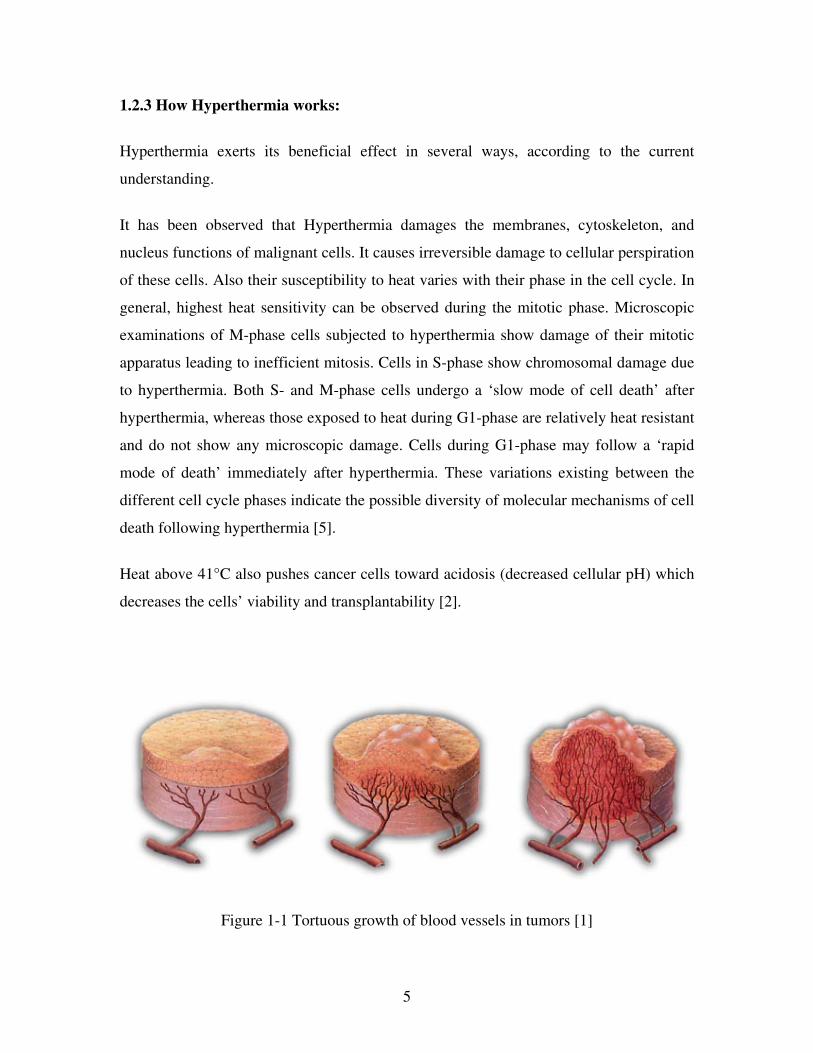
Figure 1-1 Tortuous growth of blood vessels in tumors [1]

6
As shown in Fig. 1.1, tumors have a tortuous growth of vessels feeding them blood, and
these vessels are unable to dilate and dissipate heat as normal vessels do. So tumors take
longer to heat, but then they also take longer to dissipate this heat. Also, tumor-formed
vessels do not expand in response to heat as opposed to the normal vessels which are able
to dilate in response to heat thereby causing a reduced blood flow and hence poor
dissipation of heat.
Tumor masses tend to have hypoxic (oxygen deprived) cells within the inner part of the
tumor. These cells are resistant to radiation, but they are very sensitive to heat. This is
why hyperthermia is an ideal companion to radiation: radiation kills the oxygenated outer
cells, while hyperthermia acts on the inner low-oxygen cells, oxygenating them and so
making them more susceptible to radiation damage. Moreover, hyperthermia’s induced
accumulation of proteins inhibits the malignant cells from repairing the damage
sustained.
Also, the hypoxic cells in the center of a tumor are relatively radioresistant but
thermosensitive, whereas the peripheral portions of the tumor are more sensitive to
irradiation. This supports the use of combined radiation and heat; hyperthermia is
especially effective against centrally located hypoxic cells, and irradiation eliminates the
tumor cells in the periphery of the tumor, where heat would be less effective [2].
As the research gains momentum, more reasons for the use of hyperthermia are
continuously being identified.
1.2.4 Synergistic effect of hyperthermia and radiation:
One of the most important observations from in vitro studies on heat action was that
hyperthermia and radiation act in a synergistic way. This synergism induces an increase
in cell killing even at lower temperatures, which is not the case when hyperthermia is
7
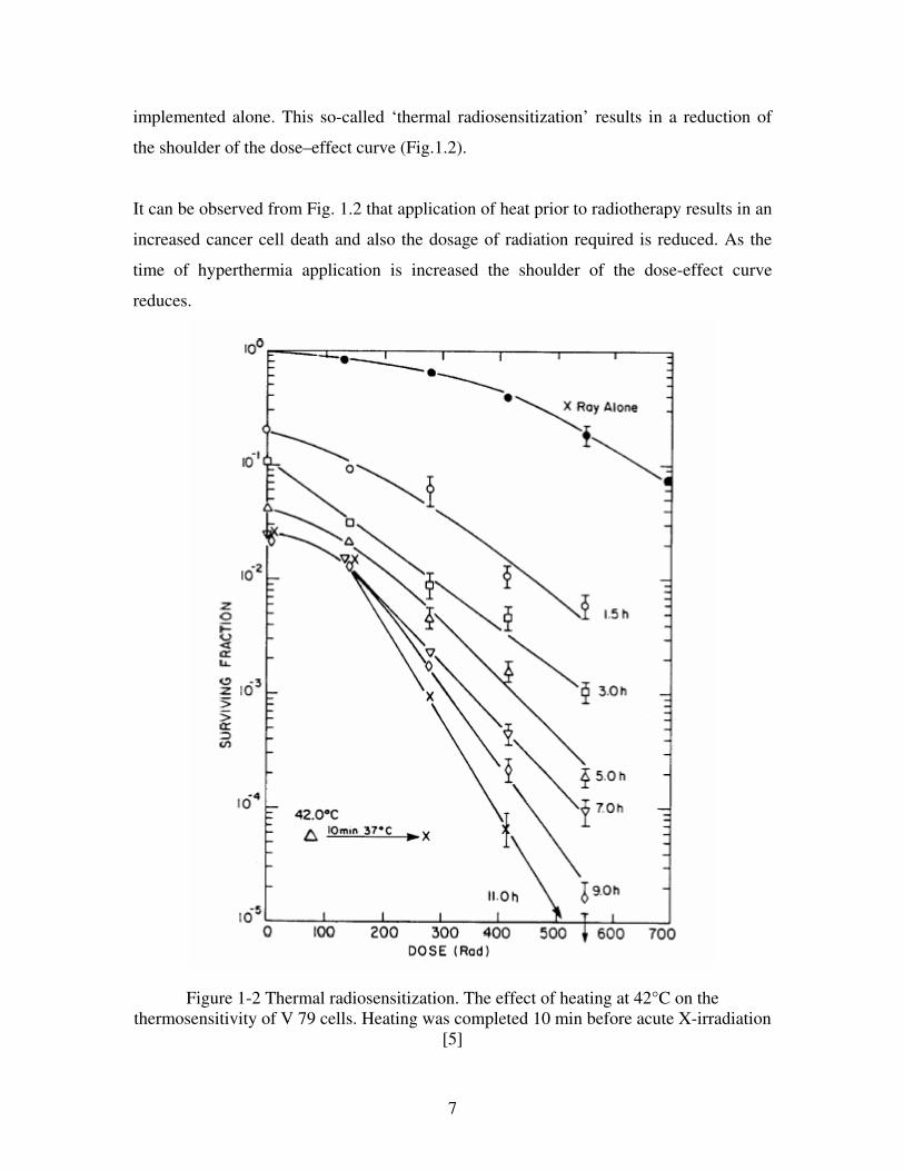
implemented alone. This so-called ‘thermal radiosensitization’ results in a reduction of
the shoulder of the dose–effect curve (Fig.1.2).
It can be observed from Fig. 1.2 that application of heat prior to radiotherapy results in an
increased cancer cell death and also the dosage of radiation required is reduced. As the
time of hyperthermia application is increased the shoulder of the dose-effect curve
reduces.
Figure 1-2 Thermal radiosensitization. The effect of heating at 42°C on the
thermosensitivity of V 79 cells. Heating was completed 10 min before acute X-irradiation
[5]

8
1.2.5 Interactions between hyperthermia and drugs:
Analogous to thermal radiosensitization, hyperthermia also enhances the cytotoxicity of
various antineoplastic agents (‘thermal chemosensitization’) [5]. Co-application of
selected chemotherapeutic drugs and hyperthermia has been shown to enhance the
inhibition of clonogenic cell growth both in vitro and in animal experiments.
1.3 Magnetic Hyperthermia
Magnetic Hyperthermia is the method of heating body tissue using magnetic materials. In
this process ferromagnetic or ferrimagnetic materials or other metals in the form of rods
or pellets are introduced near the tumor. When these are subjected to an oscillating
magnetic field, the materials are heated due to induction heating. The rate and the extent
of heating can be controlled by changing the strength and the frequency of the applied
alternating magnetic field.
Recently, a lot of work has been done in the area of magnetic hyperthermia by various
groups using a variety of materials.
• Bong Sig Koo et al. [6] have reported using steel thermoseeds as the material
which were heated inductively using a magnetic field. To evaluate the
effectiveness of the process the steel thermoseeds were implanted in rabbit liver
and tested. They have reported a maximum temperature of 54.8ºC.
• Serdar Deger et al. [7] have reported using Cobalt-Palladium thermoseeds for
treatement of prostrate cancer in combination with conformal radiation. Intra-
prostatic temperatures of 42-46ºC were obtained when these were subjected to
oscillating magnetic field.

9
• Andreas Jordan et al. have reported using Dextran-Ferrite and Dextran as
materials for magnetic hyperthermia [8]. These were tested on mammary
carcinoma of mouse.
• N. Brusentsov et al. have also reported using Dextran-Ferrite magnetic fluid
obtaining temperatures of 44-45ºC when tested in a mouse tumor [9].
The thermoseeds used for the purpose of magnetic hyperthermia have the following
major disadvantages:
• They have to be surgically inserted near the tumor. As a result the treatment
becomes complicated and also expensive.
• They do not ensure a uniform heating of the tumor. This is because the surface
area of these thermoseeds is very less. Consequently very few of the cancerous
tissue come into contact with these thermoseeds. As a result the tissue away form
the thermoseeds gets heated less effectively than that in contact with the
thermoseeds.
1.4 Hyperthermia using Magnetic Nanoparticles
The application of small particles in in vitro diagnostics has been practiced for nearly 40
years. This is due to a number of beneficial factors including a large surface area to
volume ratio, and the possibility of ubiquitous tissue accessibility. In the last decade
increased investigations and developments were observed in the field of nanosized
magnetic particles, the term nanoparticle being used to cover particulate systems that are
less than 1µm in size, and normally below 500 nm. Nanoparticles that possess magnetic
properties offer exciting new opportunities including improving the quality of magnetic
resonance imaging (MRI), hyperthermic treatment for malignant cells, site-specific drug
delivery and also the recent research interest of manipulating cell membranes [10].

10
Iron oxide magnetic nanoparticles tend to be either paramagnetic or superparamagnetic,
with particles approximately 20 nm being classed as the latter. In most cases
superparamagnetic particles are of interest for in vivo applications, as they do not retain
any magnetism after removal of the magnetic field. This is important as large domain
magnetic and paramagnetic materials aggregate after exposure to a magnetic field.
One major hurdle that underlies the use of nanoparticle therapy is the problem of getting
the particles to a particular site in the body. A potential benefit of using magnetic
nanoparticles is the use of localized magnetic field gradients to attract the particles to a
chosen site, to hold them there until the therapy is complete and then to remove them.
This involved some fairly advanced design of systems for producing these fields.
Additionally, such equipment should ideally contain other molecules to show that the
particles have been actually located in the appropriate region of the body. The particles
may be injected intravenously, and then blood circulation would be used to transport the
particles to the region of interest for treatment. Alternatively in many cases the particles
suspension would be injected directly into the general area when treatment was desired.
Either of these routes has the requirement that the particles do not aggregate and block
their own spread. [10]
1.4.1 Fate of magnetic nanoparticles following intravenous injection:
Magnetic nanoparticles are physiologically well tolerated. However the fate of
nanoparticles following intravenous administration, as indicated in Fig.1.3, represents the
diverse biological events that need to be considered. After particles are injected into the
bloodstream they are rapidly coated by components of the circulation, such as plasma
proteins. This process is known as opsonization, and is critical in dictating the
circumstance of the injected particles. Normally opsonization renders the particles
recognizable by the body’s major defense system, the reticulo-endothelial system (RES).
The RES is a diffuse system of specialized cells that are phagocytic(i.e. engulf inert
material) associated with the connective tissue framework of the liver, spleen and lymph

11
nodes. The macrophage (Kupffer) cells of the liver, and to a lesser extent the
macrophages of the spleen and circulation, therefore play a critical role in the removal of
opsonized particles. As a result, the application of nanoparticles in vivo or ex vivo would
require surface modification that would ensure particles were non-toxic, biocompatible
and stable to the RES [10].
Figure 1-3 The fate of nanoparticles following intravenous injection. Particles are
conditioned immediately on injection by plasma proteins (opsonization) [10]
Particles that have a largely hydrophobic surface are efficiently coated with plasma
components and thus rapidly removed from the circulation, whereas particles that are
more hydrophilic can resist this coating process and are cleared more slowly. This has
been used to the advantage when attempting to synthesize RES evading particles by
sterically stabilizing the particles with a layer of hydrophilic polymer chains. In the
literature the most common coatings are derivatives of dextran, polyethylene glycol
(PEG), polyethylene oxide (PEO), poloxamers and polyoxamines. The role of the dense
brushes of polymers is to inhibit opsonization, thereby permitting longer circulation
times. A further strategy in avoiding the RES is by reducing the particle. Despite all

12
efforts, however, complete evasion of the RES by these coated nanoparticles has not yet
been possible [10].
1.4.2 Heating of Magnetic Nanoparticles:
To turn these particles into heaters, they are subjected to an oscillating electromagnetic
field, where the field's direction changes cyclically. There are various theories which
explain the reasons for the heating of the magnetic nanoparticles when subjected to an
oscillating B-field.
• Application of the magnetic field generates a directional force on each magnetic
particle. When the magnetic field oscillates at high frequency switching directions
thousands to millions of times per second the direction of the force changes
according, so that the average force is zero. Creating these rotating forces requires
energy, which is taken from the oscillating magnetic field. Some of this energy
may cause the nanoparticles to rotate or vibrate. However, the cyclic nature of the
magnetic field essentially "freezes" the nanoparticles in place, preventing their net
movement in space. The remaining amount of applied energy is converted into
heat, causing the nanoparticles and their surrounding biological material to warm
up [11].
• Any metallic objects when placed in an alternating magnetic field will have
induced currents flowing within them. The amount of current is proportional to
the size of the magnetic field and the size of the object. As these currents flow
within the metal, the metal resists the flow of current and thereby heats, a process
termed inductive heating. If the metal is magnetic, such as iron, the phenomenon
is greatly enhanced. Therefore, when a magnetic fluid is exposed to an alternating
magnetic field the particles become powerful heat sources, destroying the tumor
cells [10].

13
• The heating of magnetic nanoparticles is also attributed to the hysteresis losses in
the particles [12].
1.5 Objective of the Study
Hyperthermia involves heating of the cancerous cells up to temperatures of 42-43ºC. If
heated beyond this temperature range, the normal cells are damaged which is undesirable.
The magnetic nanoparticles are heated when subjected to oscillating magnetic field. But
the temperature would increase until the particles reach the Curie temperature. A way to
overcome this problem is to regulate the magnetic field and the time of exposure to this
field i.e. to switch off the magnetic field as soon as the tissue temperature reaches the
desired range. But since the nanoparticles are spread around the tumor and lay at various
depths inside the body, they are not uniformly heated. The nanoparticles near the surface
and closer to the source of the magnetic field have the maximum temperature whereas
those located inside the body away from the source have low temperatures. Thus if the
magnetic field is switched off when the surface particles reach the optimum temperature
range, the nanoparticles inside the body are below this optimum temperature.
Consequently the efficiency of the hyperthermia process is reduced. A solution to this
problem is to use such nanoparticles so that they stop heating up after they reach the
threshold of 42ºC (315 K) however large the applied B-field may be.
1.5.1 Overview of Curie temperature:
All ferromagnetic materials have a definite temperature of transition at which the
phenomena of feromagnetism disappears and the material becomes paramagnetic. This
temperature of transition is called the “Curie temperature” or “Curie point”. Many
materials will lose essentially all of their magnetism after being heated above the Curie

14
point and then cooled. Some can be returned to the status of a permanent magnet just by
placing them in a strong magnetic field. Others require heat treatment in a strong field.
Below the Curie temperature, the ferromagnet is ordered and above it, disordered. The
saturation magnetization goes to zero at the Curie temperature. A typical plot of
magnetization vs temperature for magnetite is shown in Fig.1.4
Figure 1-4 Magnetization v/s Temperature showing Curie point [13]
A simplified explanation is that a material consists of dipoles (tiny magnetic domains) If
a magnet is cut in half you end up with two magnets. Upon repeated cutting and we get
smaller magnets each with a north-south pole until theoretically the size of a dipole is
reached. In a mass of material those dipoles are pointed in random directions but have
some (if limited) movement. If the material is placed in a strong magnetic field the
dipoles can be forced to line up as N-s,n-s,n-s,n-S where the capitals are at the end of the
piece. If the field is now removed, some materials will keep the dipoles lined up and we
get a permanent magnet with a North and South Pole. Some don't remain lined up and are
considered soft magnetic materials [14].
15
If the magnet is hammered or heated and then cooled without a magnetic field the dipoles
may randomize again because they get the freedom to move and lose the magnetism.
Some hard magnetic materials need to be heated (to allow the dipoles to rotate around)
and then cooled in a strong magnetic field to attain maximum magnetization. The heat
treatment program can be fairly complex. The Alnico magnets are in this category.
Permanent magnets are materials which can lock dipoles in position just like some crystal
structures can be locked in place. Just as a particular heat treatment can create different
degrees of hardness e.g. some special heat treatments can produce different magnetism in
a material. If heated again, they can lose the magnetism. Soft magnetic materials lose
their magnetism as soon as the magnetic field is removed [14].
1.5.2 Self controlled hyperthermia:
This magnetic property of Curie temperature can be utilized to overcome the problems of
uneven heating and temperature regulation. If the material of the magnetic nanoparticles
has a Curie temperature in the optimum heating range 42-43ºC then if they are subjected
to oscillating magnetic field the temperature of these will rise only up to its Curie
temperature. If they are further subjected to the magnetic field of any intensity they won’t
be heated thereafter because beyond the Curie temperature the nanoparticles become
paramagnetic.
This will also ensure a uniform heating because now the magnetic field can be kept on till
all the particles irrespective of their depth inside the body reach the optimum temperature
which corresponds to their curie temperature.
If nanoparticles with Curie temperature of 42-43ºC are used then there would be no need
to regulate the applied field. As a result the cost of the equipment will also reduce.

16
1.5.3 Quest for magnetic nanoparticles with Tc=42-43ºC:
The objective of the thesis is to find a suitable magnetic material which will exhibit Curie
temperature in the optimum range 42-43 ºC. For this a wide variety of magnetic
compounds were explored. They were synthesized using mainly chemical means and
were then tested for their Curie temperature.
1.5.4 Biocompatibility issue:
Another requirement for the magnetic nanoparticles is that they should be bio-
compatible. If non bio-compatible particles are injected into the body there may be
problems of toxicity. So in this thesis the various magnetic nanoparticles explored were
all of bio-compatible elements. Only those elements were used which are present in the
human body naturally e.g. Fe, Ni, Mn, Zn etc.
1.5.5 Polymer/Protein coating:
The particles need to be encapsulated within biocompatible polymers/proteins to make
them appear friendly to the body. The coatings ensure that the particles are not quickly
eliminated by the RES and hence are sustained in the body for a long time. The
polymer/protein used to encapsulate the particles could be such that they melt and break
open at 42°C. These polymers/proteins are knows as heat sensitive polymers/proteins.
Also, a suitable drug (chemotherapy drug or radiosensitizer) can be loaded inside these
coatings along with the magnetic nanoparticles. Thus the Polymer/protein capsule acts as
a carrier for the magnetic nanoparticles and a suitable drug.

17
1.5.6 Testing of the coated nanoparticles:
The morphology of the coated nanoparticles were observed using a TEM. The
nanoparticles coated with polymer/protein were checked to ensure that they are heated to
upto 42°C when subjected to an alternating magnetic field. Also experiments were
performed to confirm that the coatings were lysed open at 42°C.
1.6 Scope of the study
For attaining the objective mentioned in the previous section the following tasks are to be
completed:
1 Preparation of Magnetic nanoparticles using bio-compatible elements using
physical or chemical means. These include:
a) Fe-Zn Ferrite nanoparticles
b) Mn-Zn Ferrite nanopartices
c) Gd substituted Mn-Zn Ferrite nanoparticles
d) Zn Ferrite nanoparticles
e) Gd substituted Zn Ferrite nanoparticles
f) Ni-Cu nanoparticles
g) Gd4C nanoparticles
2 Investigation of their Curie temperature to check whether it is in the range 42-
43°C
3 Encapsulation of the particles within the following polymers/proteins:
a) Polyethylene glycol
b) Ethyl cellulose
c) Polyvinyl alcohol
d) Human serum albumin
4 Observing the morphology of the encapsulated particles under TEM to ensure
proper coating

18
5 Experimental testing of the encapsulated magnetic nanoparticles for heating upto
42°C when subjected to alternating magnetic field
6 Experimental testing of the encapsulated magnetic nanoparticles for breaking of
coatings at 42°C.
Chapter 1 was a brief introduction to cancer, the common modalities used to treat cancer,
hyperthermia especially magnetic hyperthermia. In chapter 2 the chemical and physical
methods or procedures used to synthesize magnetic nanoparticles in this study have been
discussed. Chapter 3 describes the various instruments such as SQUID, VSM, XRD,
TEM, BI-MAS, used for characterizing the magnetic nanoparticles synthesized. In
chapter 4 the different types of magnetic nanoparticles synthesized in this study have
been discussed in details. The methods of their synthesis and their characterization results
have also been presented in this chapter. Chapter 5 deals with the encapsulation of the
magnetic nanoparticles within polymers/proteins. The different polymers/proteins used
and their respective methods for coating the particles have been presented in details.
Chapter 6 concludes this work and states the future work possible to extend this study.
Also Appendix A is a general information about cancer, its causes and the different types
of cancer.

19
CHAPTER 2
SYNTHESIS TECHNIQUES
This chapter presents the various chemical and physical methods which were used to
synthesize magnetic nanoparticles in this study. The elements chosen for the material of
the nanoparticles were bio-compatible. Each of these elements is present in the human
body as trace elements or in large quantities.
2.1 Chemical Methods
Chemistry has played a major role in developing new materials with novel
technologically important properties. The advantage of chemical synthesis is its
versatility in designing and synthesizing new materials that can be refined into the final
product. The primary advantage that chemical processes offer over other methods is good
chemical homogeneity, as chemical synthesis offers mixing at the molecular level.
Molecular chemistry can be designed to prepare new materials by understanding how
matter is assembled on an atomic and molecular level and the consequent effects on the
desired material macroscopic properties. A basic understanding of the principles of
crystal chemistry, thermodynamics, phase equilibrium, and reaction kinetics is important
to take advantage of the many benefits that chemical processing has to offer.
However, there are certain difficulties in chemical processing. In some preparations, the
chemistry is complex and hazardous. Contamination can also result from byproducts
being generated or side reactions in the chemical process. This should be minimized or

20
avoided to obtain desirable properties in the final product. Agglomeration can also be a
major cause of concern at any stage in a synthetic process and it can drastically alter the
properties of the materials. Finally, although many chemical processes are scalable for
economical production, it is not always straightforward for all systems [15].
Precipitation of a solid from a solution is a common technique for the synthesis of fine
particles. The general procedure involves reactions in aqueous or non aqueous solutions
containing the soluble or suspended salts. Once the solution becomes supersaturated with
the product, the precipitate is formed by either homogeneous or heterogeneous
nucleation. The formation of nuclei after formation usually proceeds by diffusion in
which case concentration gradients and reaction temperatures are very important in
determining the growth rate of the particles, for example, to form monodispersed
particles. For instance, to prepare unagglomerated particles with a very narrow size
distribution, all the nuclei must form at nearly the same time and subsequent growth must
occur without further nucleation or agglomeration of the particles.
In general, the particle size and particle size distribution, the physical properties such as
crystallinity and crystal structure, and the degree of dispersion can be affected by reaction
kinetics [15, 16]. In addition, the concentration of reactants, the reaction temperature, the
pH, and the order of addition of reactants to the solution are also important. Even though
a multielement material is often made by co-precipitation of batched ions, it is not always
easy to co-precipitate all the desired ions simultaneously because different species may
only precipitate at different pH. Thus, control of chemical homogeneity and
stoichiometry requires a very careful control of reaction conditions [15].
2.1.1 Borohydride reduction:
In this method, salts of the required metallic elements are reduced by sodium borohydride
(NaBH4). The procedure involves a dropwise addition of aqueous solution of metallic
salts to NaBH4 solution along with a vigorous stirring. The pH of the salt solution is
21
maintained at 6 whereas that of the NaBH4 is maintained at 12. NaOH can be added to
the NaBH4 solution to increase the pH to this level.
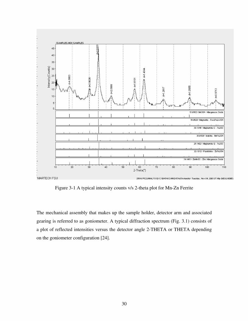
Fe-Gd-B nanoparticles were synthesized using this method. A 0.04 M solution of salts
GdCl3 and FeSO4 mixed in the required stoichiometric proportions was added to a 1 M
NaBH4 solution kept in a round bottom flask. The resultant mixture was vigorously
stirred. Also the reaction was carried out in an atmosphere of argon by passing argon into
the flask during the reaction. After complete addition of the salt solution, the reaction and
stirring was allowed to continue for 40 minutes more. The reaction could be represented
by the following chemical reaction:
( ) .42234434 etcSONaOHHClFeClGdSOBGdFeNaBHGdClFeSOArgon ++++++−−⎯⎯ →⎯++
3 samples were made with Gd:Fe ratios of 80:20, 60:40 and 95:5. Fe-Nd-B particles are
usually synthesized using this method. But it has a very high curie temperature of 310ºC
[17], well beyond the required optimum range of 42-43ºC. So an attempt was made to
replace Nd with Gd with an aim of bringing down the Curie temperature.
2.1.2 Chemical coprecipitation method:
In this process the salt solution of the required metallic elements is reduced by NaOH
solution. The reactants when mixed are at temperatures of 90ºC. After the mixing the
reaction is continued for 40 minutes along with heating at 90ºC.
Chemical co-precipitation is widely used to synthesize Ferrite (Fe3O4) nanoparticles. It is
also used to make many other Ferrites such as Zn Ferrite, Mn-Zn Ferrite, Cu Ferrite etc.
Ferrite fine particles are obtained by the co-precipitation from aqueous solutions of
trivalent Fe3+
and bivalent metal Me2+
, where Fe2+
, Mn2+
, Co2+
, Ni2+
and/or Zn2+
may
serve as Me2+
. The initial molar proportion (Me2+
/Fe3+
) is always taken as the
stoichiometric ½.

22
The co-precipitation reaction takes place in two steps:
1. Co-precipitation step: At first solid hydroxides of metals in the form of colloidal
particles are obtained by the co-precipitation of metal cations in alkaline medium.
For the case of Mn-Zn Ferrite this reaction is as follows:
−+++ +++− OHFexZnMnx 82)1( 322
322 )(2.)(.)()1( OHFeOHxZnOHMnx−
2. Ferritisation step: Then this product is subjected to heating in the precipitation
alkaline solution to provide the transformation of solid solution of metal
hydroxides to the Mn-Zn Ferrite
322 )(2.)(.)()1( OHFeOHxZnOHMnx−
OHnOnHOFeZnMn xx 2242)1( )4(. −+−
A particular feature of “the co-precipitation method” is that the product contains a certain
amount of associated water even after several hours of heating in alkaline solution [16].
The rate of mixing of reagents plays a vital role in the size of the resultant particles. Co-
precipitation consists of two processes: nucleation (formation of centers of
crystallization) and a subsequent growth of particles. The relative rates of these two
processes determine the size and polydispersity of obtained particles. Polydispersed
colloids are obtained as a result of simultaneous formation of new nuclei and growth of
the earlier formed particles. Less dispersed in size colloid is formed when the rate of
nucleation is high and the rate of particles growth is low. This situation corresponds to a
rapid addition and a vigorous mixing of reagents in the reaction [16].

23
Slow addition of reagents in the coprecipitation reaction leads to the formation of bigger
nuclei than rapid one. It must be also taken into account that in the case of slow addition
of the base to solution of metal salts a separate precipitation takes place due to the
different pH of precipitation pHpr for different metals. Separate precipitation may
increase the chemical inhomogenity in the particles. To obtain ferrite particles of a
smaller size, less dispersed in size and more chemically homogeneous the mixing of
reagents must be performed as fast as possible [16].
An increase in temperature (in the range 20-100°C) significantly accelerates formation of
ferrite particles. The activation energy for formation of ferrites of different metals is not
equal. Auzans et al. [16] conclude that the heating at temperatures close to 100°C is
preferable for an easier and more rapid formation of the Mn-Zn ferrite particles.
Following nanoparticles were synthesized using the chemical co-precipitation method:
• Mn-Zn Ferrite: In Ref [16] the authors had claimed that the curie temperature of
the Mn-Zn Ferrite nanoparticles was in the range 370-523 K for various Zn
proportions. So in this work an attempt was made to synthesize Mn-Zn Ferrite
nanoparticles with curie temperatures in the desired range of 315 K (42ºC) by
changing the Zn proportions.
• Gd-substituted Mn-Zn Ferrite: In ref [18] the authors had substituted Gd in the
Mn-Zn Ferrite nanoparticles with Mn:Zn=1:1 ratio. They had claimed that the
curie temperature of the resultant particle was 348 K. So in this work an attempt
was made to synthesize Gd substituted Mn-Zn Ferrite nanoparticles with Mn:Zn
ratio other than 1:1 with an aim of bringing the curie temperature in the desired
range of 315 K.
• Fe-Zn Ferrite: Fe-Zn Ferrite particles of the form ZnxFe1-xFe2O4 were
synthesized by authors in the ref [19] using chemical co-precipitation. They had
found the curie temperature of these particles to be 364 K for x = 0.5 and 347 K
for x = 0.7. In this work similar Fe-Zn Ferrite nanoparticles were synthesized with
x >= 0.7 with an aim of getting the Curie temperature down to the desired range
of 315 K.

24
• Zn Ferrite: From the trend of Curie temperature of the Fe-Zn Ferrite
nanoparticles it was observed that the curie temperature of the nanoparticles
decreased with increasing Zn proportions. So Zn-Ferrite particles were
synthesized using chemical co-precipitation with the hope of getting the Tc in the
desired range of 315 K.
• Gd-substituted Zn Ferrite: On comparing the characterization data of the Gd-
substituted Mn-Zn Ferrite particles with that of the Mn-Zn Ferrite particles it was
noticed that addition of Gd in small amounts leads to an increase in the Curie
temperature as well as the pyromagnetic co-efficient of the nanoparticles. Since
the Curie temperature of the Zn Ferrite was measured to be below the desired
range, Gd-substituted Zn Ferrie particles were synthesized to increase its curie
temperature.
2.1.3 Refluxing in polyol method
In this method, liquid polyols such as ethylene glycol or diethylene are used both as a
solvent and as a reducing agent for the chemical preparation of metallic powders from
various inorganic precursors [20]. The basic reaction scheme for the synthesis of these
metal powders by the polyol process involves:
• dissolution of the solid precursor
• reduction of the dissolved metallic species by the polyol itself
• nucleation of the metallic phase
• growth of the nuclei
To obtain metallic powders with a narrow size distribution, two conditions must be
fulfilled:
1. A complete separation of the nucleation and growth steps is required and
2. The aggregation of metal particles must be avoided during the nucleation
and growth steps.

25
The general procedure for the synthesis of different metallic powders and films involved
suspending the corresponding metal precursors in ethylene glycol or tetraethylene glycol
and subsequently bringing the resulting mixture to refluxing temperature (generally
between 120 to 200°C) for 1 - 3 hr. During this reaction time, the metallic moieties are
precipitated out of the mixture. The metal-glycol mixture is then cooled to room
temperature, filtered, and the collected precipitate is dried in air. For film deposition,
substrates are immersed in the reaction mixture [21].
Compared to aqueous methods, the polyol approach results in synthesis of metallic
nanoparticles protected by surface adsorbed glycol, thus minimizing the oxidation
problem [22].
Lilly et al. [23] have synthesized Ni-Cu thermoseeds using physical means for
application in hyperthermia. The Ni-Cu alloy synthesized was of proportion
Ni:Cu=70.4:29.6. The authors claimed that the Ni-Cu thermoseeds had a Curie
temperature of 50ºC.
In this work, Ni-Cu nanoparticles were synthesized using the polyol process. The salts
NiCl2 and CuSO4 were dissolved in ethylene glycol and refluxed at 195ºC for 11-12 hrs.
2.2 Physical Methods
One of the physical methods of synthesizing magnetic nanoparticles involves arc melting
of the constituent metals in an inert furnace. The high temperatures necessary for melting
are produced by creating an electric arc. This requires the melting take place in an inert
atmosphere usually that of argon.

26
In this work Gd4C was synthesized by melting Gd and Carbon in the required ratio in an
arc furnace. The result was a solid Gd4C ingot. This was then broken down into pieces
using mechanical means and then reduced to nanosize using an ultrasonicator.
2.3 Comparison of the Synthesis Methods
The chemical synthesis methods such as borohydride reduction, chemical co-precipitation
and polyol method, have several advantages over the physical methods:
• At the end of the process the material is obtained directly in nanosize whereas in
the physical methods the ingots have to be broken down into nano size using other
means such as ball milling, sputtering etc.
• The chemical processes ensure mixing at molecular level whereas the physical
methods do not.
• The chemical processes mentioned above are scalable for commercial
manufacturing as opposed to the physical methods which require a high
temperature arc furnace. Besides the arc furnace requires vacuum in the melting
chamber which is difficult if the chamber size has to be big for commercial
production.
2.3 Summary
This chapter presented a brief introduction about the different chemical and physical
methods used in this study to synthesize magnetic nanoparticles. Also, comparing the
chemical and physical methods it can be observed that the chemical methods have a
definite advantage over the physical methods mainly due to the mixing of constituents
at molecular level and the ability to produce nanosized particles directly. In chapter 4

27
the above procedures have been discussed in details for each type of nanoparticles
synthesized.

28
CHAPTER 3
EXPERIMENTAL METHODS FOR CHARACTERIZATION OF
MAGNETIC NANOPARTICLES
This chapter describes the various instruments and methods used for the characterization
of the Magnetic nanoparticles synthesized in this study. These involve the instruments for
determining the magnetic properties such as Curie temperature and Magnetic saturation
(SQUID and VSM) as well as those for determining the approximate chemical contents
of the particles (XRD). The instruments XRD, VSM and SQUID used in this study were
located at MARTECH, FSU whereas the TEM was located at NHMFL, Tallahassee and
at the Biology dept. FSU.
3.1 X-Ray Diffractometer (XRD)
About 95% of all solid materials can be described as crystalline. When X-rays interact
with a crystalline substance (Phase), one gets a diffraction pattern. In 1919 A.W.Hull
gave a paper titled, “A New Method of Chemical Analysis”. Here he pointed out that
“….every crystalline substance gives a pattern; the same substance always gives the same
pattern; and in a mixture of substances each produces its pattern independently of the
others. “ The X-ray diffraction pattern of a pure substance is, therefore, like a fingerprint
of the substance. The powder diffraction method is thus ideally suited for characterization
and identification of polycrystalline phases. Today about 50,000 inorganic and 25,000
organic single component, crystalline phases, diffraction patterns have been collected and

29
stored on magnetic or optical media as standards. The main use of powder diffraction is
to identify components in a sample by a search/match procedure. Furthermore, the areas
under the peak are related to the amount of each phase present in the sample [24].
Solid matter can be described as:
• Amorphous: The atoms are arranged in a random way similar to the disorder we
find in a liquid. Glasses are amorphous materials.
• Crystalline: The atoms are arranged in a regular pattern, and there is as smallest
volume element that by repetition in three dimensions describes the crystal. E.g.
we can describe a brick wall by the shape and orientation of a single brick. This
smallest volume element is called a unit cell. The dimensions of the unit cell is
described by three axes: a, b, c and the angles between them alpha, beta, gamma.
About 95% of all solids can be described as crystalline.
An electron in an alternating electromagnetic field will oscillate with the same frequency
as the field. When an X-ray beam hits an atom, the electrons around the atom start to
oscillate with the same frequency as the incoming beam. In almost all directions we will
have destructive interference, that is, the combining waves are out of phase and there is
no resultant energy leaving the solid sample. However the atoms in a crystal are arranged
in a regular pattern, and in a very few directions we will have constructive interference.
The waves will be in phase and there will be well defined X-ray beams leaving the
sample at various directions. Hence, a diffracted beam may be described as a beam
composed of a large number of scattered rays mutually reinforcing one another.
The X-rays are reflected from a series of parallel planes inside the crystal. The orientation
and interplanar spacings of these planes are defined by the three integers h, k, and l called
indices. A given set of planes with indices h, k, and l cut the a-axis of the unit cell in h
sections, the b axis in k sections and the c axis in l sections. A zero indicates that the
planes are parallel to the corresponding axis. E.g. the 2, 2, 0 planes cut the a– and the b–
axes in half, but are parallel to the c– axis.
30
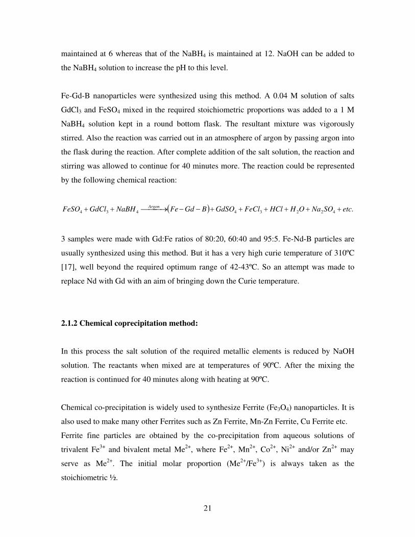
Figure 3-1 A typical intensity counts v/s 2-theta plot for Mn-Zn Ferrite
The mechanical assembly that makes up the sample holder, detector arm and associated
gearing is referred to as goniometer. A typical diffraction spectrum (Fig. 3.1) consists of
a plot of reflected intensities versus the detector angle 2-THETA or THETA depending
on the goniometer configuration [24].

31
3.2 Vibrating Sample Magnetometer
The VSM is based upon Faraday’s law according to which an e.m.f. is induced in a
conductor by a time-varying magnetic flux. In VSM, a sample magnetized by a
homogenous magnetic field is vibrated sinusoidally at small fixed amplitude with respect
to stationary pick-up coils (Fig. 3.2). The resulting field change at a point inside the
detection coils induces voltage. This voltage can be detected to a high resolution and
accuracy by means of suitable associated electronics. For stationary pick-up coils and a
uniform and stable external field, the only effect measured by the coils is that due to the
motion of the sample. The voltage is thus a measure of the magnetic moment of the
sample [25].
Figure 3-2 Principle of working of VSM [25]

32
In this study, the VSM at Martech, FSU was used to determine hysteresis plots of the
samples. From the hysteresis plots the saturation magnetization was determined. A
typical hysteresis plot obtained from VSM is shown in Fig. 3.3
Figure 3-3 A typical hysteresis curve for Mn-Zn Ferrite nanoparticles obtained using
VSM

33
3.3 Superconducting QUantum Interference Device (SQUID)
A superconducting quantum interference device (SQUID) is a mechanism used to
measure extremely weak signals, such as subtle changes in the human body's
electromagnetic energy field. Using a device called a Josephson junction, a SQUID can
detect a change of energy as much as 100 billion times weaker than the electromagnetic
energy that moves a compass needle. A Josephson junction is made up of two
superconductors, separated by an insulating layer so thin that electrons can pass through.
A SQUID consists of tiny loops of superconductors employing Josephson junctions to
achieve superposition: each electron moves simultaneously in both directions. Because
the current is moving in two opposite directions, the electrons have the ability to perform
as qubits (that theoretically could be used to enable quantum computing). SQUIDs have
been used for a variety of testing purposes that demand extreme sensitivity, including
engineering, medical, and geological equipment. Because they measure changes in a
magnetic field with such sensitivity, they do not have to come in contact with a system
that they are testing [26].
SQUIDs are usually made of either a lead alloy (with 10% gold or indium) and/or
niobium, often consisting of the tunnel barrier sandwiched between a base electrode of
niobium and the top electrode of lead alloy. A radio frequency (RF) SQUID is made up
of one Josephson junction, which is mounted on a superconducting ring. An oscillating
current is applied to an external circuit, whose voltage changes as an effect of the
interaction between it and the ring. The magnetic flux is then measured. A direct current
(DC) SQUID, which is much more sensitive, consists of two Josephson junctions
employed in parallel so that electrons tunneling through the junctions demonstrate
quantum interference, dependent upon the strength of the magnetic field within a loop.
DC SQUIDs demonstrate resistance in response to even tiny variations in a magnetic
field, which is the capacity that enables detection of such minute changes [26].

34
Figure 3-4 A typical plot of temperature dependence of magnetization obtained using
SQUID
A SQUID is capable of detecting magnetic fields of around 2 pT. It has however been
demonstrated that fields of around 100 fT are also within the scope of a SQUID. It is
typically required to be kept at temperatures of around 4.2 Kelvin [27].
In this study, the SQUID was used to determine the Curie temperature of the particles
from the temperature dependence of magnetization plots. It is a plot of the Long Moment
(EMU) v/s the temperature (K). A typical plot of the data obtained from the SQUID is
shown in Fig. 3.4. The point where the extrapolated linear portion of the data meets the
X-axis is the Curie temperature for the particle.

35
3.4 Transmission Electron Microscope (TEM)
A JEOL-2010 TEM located at NHMFL, Tallahassee and a Philips CM300 FEG TEM
located at Biology dept. of FSU were used in this study to observe the structure of the
nanoparticles synthesized.
A TEM works much like a slide projector. A projector shines (transmits) a beam of light
through the slide, as the light passes through it is affected by the structures and objects on
the slide. These effects result in only certain parts of the light beam being transmitted
through certain parts of the slide. This transmitted beam is then projected onto the
viewing screen, forming an enlarged image of the slide.
TEMs work the same way except that they shine a beam of electrons (like the light)
through the specimen (like the slide). Whatever part is transmitted is projected onto a
phosphor screen for the user to see. A more technical explanation of a typical TEMs
working is as follows (Fig. 3.5):
1. The "Virtual Source" at the top represents the electron gun, producing a stream of
monochromatic electrons.
2. This stream is focused to a small, thin, coherent beam by the use of condenser
lenses 1 and 2. The first lens (usually controlled by the "spot size knob") largely
determines the "spot size"; the general size range of the final spot that strikes the
sample. The second lens(usually controlled by the "intensity or brightness knob"
actually changes the size of the spot on the sample; changing it from a wide
dispersed spot to a pinpoint beam.
3. The beam is restricted by the condenser aperture (usually user selectable),
knocking out high angle electrons (those far from the optic axis, the dotted line
down the center)

36
Figure 3-5 Principle of working of a TEM [28]
4. The beam strikes the specimen and parts of it are transmitted
5. This transmitted portion is focused by the objective lens into an image
6. Optional Objective and Selected Area metal apertures can restrict the beam; the
Objective aperture enhancing contrast by blocking out high-angle diffracted
electrons, the Selected Area aperture enabling the user to examine the periodic
diffraction of electrons by ordered arrangements of atoms in the sample
7. The image is passed down the column through the intermediate and projector
lenses, being enlarged all the way

37
8. The image strikes the phosphor image screen and light is generated, allowing the
user to see the image. The darker areas of the image represent those areas of the
sample that fewer electrons were transmitted through (they are thicker or denser).
The lighter areas of the image represent those areas of the sample that more
electrons were transmitted through (they are thinner or less dense) [28]
For the observation of the nanoparticles, a dilute solution of the particles in acetone was
prepared. Two drops of this solution were then dropped on the copper grids which acted
as the specimen in TEM.
3.5 BIC 90Plus/BI-MAS
The multi angle particle sizing option in a BIC ZetaPals was used to measure the
approximate diameter of the particles and their size distribution.
The MAS OPTION is an automatic particle sizer designed for use with either
concentrated suspensions of small particles or solutions of macromolecules. Generally
speaking, sizes from 2nm to 3µm can be measured. The technique involved – photon
correlation spectroscopy (PCS) of quasi elastically scattered light (QELS) – is based on
correlating the fluctuations about the average, scattered, laser light intensity. The
specifications for this machine were as follows:
Size Range : 2nm to 3µm
Accuracy : ±1% to 2% with monodisperse samples
Repeatability : ± 1% to 2% with dust free samples
Sample Volume : 0.5 to 3ml
Measurement Time : Typically 1 to 2 mins
Results : Mean and Standard Deviation calculated for size
distribution by weight assuming a Lognormal distribution.

38
The explanation of the working principle of this instrument as given in the BI-MAS
OPTION manual is: Light may be treated as an electromagnetic wave. The oscillating
electron-magnetic field induces oscillations of the electrons in a particle. These
oscillating changes form the source of the scattered light. Over the years many features of
the scattered light have been used to determine particle size. These include:
• Changes in the average intensity as a function of angle
• Changes in the polarization
• Changes in the wavelength
• Fluctuations about the average intensity
This later phenomenon is the basis for QELS, the technique employed in the MAS
OPTION, and it arises in the following manner: imagine a detector of light fixed as some
angle with respect to the direction of the incident light beam and at some fixed distance
from the scattering volume which contains a large number of particles. Scattered light
from each particle reaches the detector. Since the small particles are moving randomly in
the liquid, undergoing diffusive Brownian motion, the distance that the scattered waves
travel to the detector varies as a function of time. Electromagnetic waves, like water and
sound waves, exhibit interference effects. Scattered waves can interfere constructively or
destructively depending on the distances traveled to the detector. The result is an average
intensity with superimposed fluctuations.
The decay times of the fluctuations are related to the diffusion constants and, therefore,
the sizes of the particles. Small particles moving rapidly cause faster decaying
fluctuations than larger particles moving slowly. The decay times of these fluctuations
may be determined either in the frequency domain (using a spectrum analyzer) or in the
time domain (using a correlator). The correlator generally offers the most efficient means
for this type of measurement.
In QELS the total time over which a measurement is made is divided into small time
intervals called delay times. These intervals are selected to be small compared with the

39
time it takes for a typical fluctuation to relax back to the average. The scattered light
intensity in each of these intervals, as represented by the number of electrical pulses
registered during each delay time, fluctuates about a mean value. The intensity
autocorrelation function is formed by averaging the products of the intensities in these
small time intervals as a function of the time between the intervals (delay times). A
computer automatically controls the buildup of the function including the choice of delay
times, the length of the experiment, and display of pertinent information, data analysis,
and the printing of results.
3.5 Summary
In this chapter the principles of workings of the various instruments used for the
characterization of the nanoparticles were described. The SQUID and the VSM were
used for characterization of magnetic properties whereas the XRD and TEM were used
for chemical analysis and morphological characterization respectively. Also, the ZetaPals
BI-MAS OPTION was used to get an estimate of the average particle size and size
distribution

40
CHAPTER 4
RESULTS AND DISCUSSION
This chapter presents the various magnetic nanoparticles synthesized in this study with an
aim to find a material which will have a Curie temperature of 42ºC (315 K). It also puts
forward the motivation behind the synthesis of each of these particles and their
characterization results.
4.1 Fe-Gd-B Nanoparticles by Borohydride Reduction
4.1.1 Motivation:
Borohydride reduction method is widely used to synthesize nanoparticles containing
boron. D. Fiorani et al. [29] have synthesized Fe-Cr-B nanoparticles using this method.
The resultant particles in this report [29] were mostly antiferromagnetic with a maximum
Neel temperature of 77 K. G. D. Forster et al. [30] have synthesized Fe-Mn-B
nanoparticles using the borohydride reduction method. Also P. Fulmer et al [31] have
synthesized Fe-Co-B nanoparticles using this method. Fe-Nd-B which is widely used in
industry has a very high Curie temperature of 310ºC [17].
In this study the motivation for synthesizing Fe-Gd-B nanoparticles using the
borohydride reduction method was to try to bring down the Curie temperature to the
41
desired 315 K by replacing the rare earth metal Neodymium in Fe-Nd-B with another
Rare earth metal Gadolinium which has a Curie temperature of 298 K.
The experimental procedure for this method is explained in chapter 2, section 2.1.1.
4.1.2 Characterization results:
Three samples of Fe-Gd-B were synthesized using borohydride reduction method. Their
characterization led to the following results
1. Fe-Gd-B with Gd:Fe = 95:5:
Figure 4-1 Temperature dependence of magnetization for Fe-Gd-B (Gd:Fe=95:5)

42
2. Fe-Gd-B with Gd:Fe = 80:20
Figure 4-2 Temperature dependence of magnetization for Fe-Gd-B (Gd:Fe=80:20)
3. Fe-Gd-B with Gd:Fe = 60:40
This sample was found to be unstable and was hence discarded.
4.1.3 Discussion of results:
The Curie temperatures for the Fe-Gd-B samples were found to be well beyond the
measuring range of the SQUID but by approximately extrapolating the plots it was
observed that if the proportion of Gd was increased the Curie temperature of the resultant
nanoparticles was decreased. This can be attributed to the fact that the Curie temperature
of Gd is 298 K which is much lower than that of Fe (1043 K)

43
However, the Curie temperatures were much higher than the desired optimum 315 K for
hyperthermia application. Thus the Fe-Gd-B particles were found to be unfit for use in
hyperthermia using magnetic nanoparticles.
4.2 Mn-Zn Ferrite Nanoparticles by Chemical Co-precipitation
4.2.1 Motivation:
Mn-Zn Ferrite has recently gained a lot of interest mainly because of the ability to change
its properties by varying the proportions of its constituents. Auzans et al. [16] have
synthesized Mn-Zn nanoparticles using the chemical co-precipitation method in which
the proportions of Zinc were varied and the effects on the properties were studied. The
Curie temperatures of their particles were above the desired 315 K. For zinc proportions
x = 0.78 they had obtained a Curie temperature of 370 K which was closest to the desired
315 K than their other particles.
In this study several Mn-Zn Ferrite particles with various constituent proportions were
synthesized to check whether it is possible to bring down the Curie temperature to the
desired 315 K.
4.2.2 Method of preparation:
Several samples of the form 42)1( OFeZnMn xx− were synthesized using chemical
co-precipitation method. In this method a 0.1 M solution of the metal salts MnCl2,
Fe2SO4 and ZnSO4 was added to an 8 M solution of NaOH. The mixture was stirred
vigorously at 90ºC for 40 mins. Thereafter the synthesized nanoparticles were filtered and

44
washed 3 times with distilled water and 3 times with acetone. The particles were then
allowed to dry in air at room temperature.
4.2.3 Characterization results:
The characterization results of a significant few amongst them are presented below:
1. Mn-Zn Ferrite with x = 0.5
Figure 4-3 Temperature dependence of magnetization for Mn-Zn Ferrite with x=0.5

45
Figure 4-4 Hysteresis curve for Gd-Mn-Zn Ferrite with x = 0.5
2. Mn-Zn Ferrite with x = 0.6
Figure 4-5 Temperature dependence of magnetization for Mn-Zn Ferrite with x=0.6
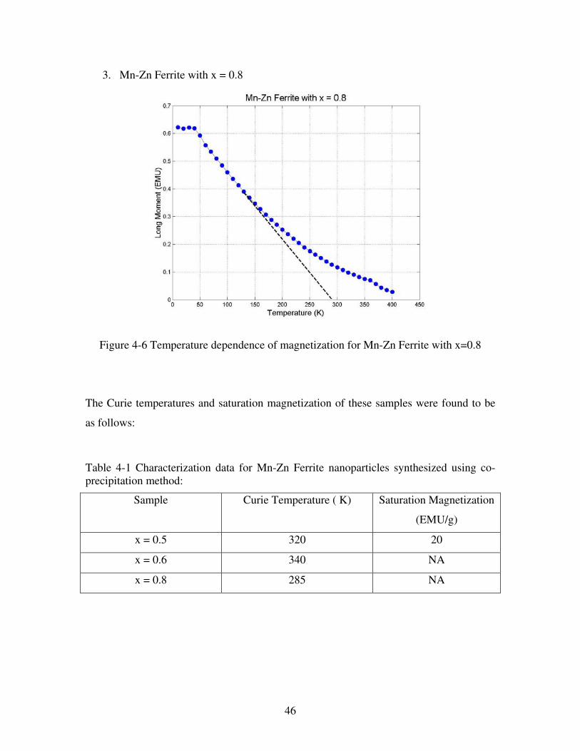
46
3. Mn-Zn Ferrite with x = 0.8
Figure 4-6 Temperature dependence of magnetization for Mn-Zn Ferrite with x=0.8
The Curie temperatures and saturation magnetization of these samples were found to be
as follows:
Table 4-1 Characterization data for Mn-Zn Ferrite nanoparticles synthesized using co-
precipitation method:
Sample Curie Temperature ( K) Saturation Magnetization
(EMU/g)
x = 0.5 320 20
x = 0.6 340 NA
x = 0.8 285 NA

47
4.2.4 Discussion of results:
It was observed that the Curie temperature of the particles decreases for zinc proportions
x > 0.6. The Zinc atoms tend to occupy the smaller tetrahedral sites [32] and hence
displace the Mn atoms at those sites. Since Zn does not contribute to the magnetic
moment due to its filled 3d and 4s shells, it results in a weakening of the net magnetic
moment of the particles thereby decreasing the B-B interaction and hence the Curie
temperature.
The Curie temperature of the sample with x = 0.5 was found to be close to the desired
315 K. The Curie temperatures of other samples were either below or above this
temperature.
4.3 Gd substituted Mn-Zn Ferrite Nanoparticles
4.3.1 Motivation:
Upadhyay et al. [18] have synthesized Gd substituted Mn-Zn Ferrite nanoparticles using
chemical co-precipitation. They observed an increase in the pyromagnetic co-efficient
( HTM )/( ∂∂ ) of the resultant particles. The increase in the pyromagnetic co-efficient is
desirable because it results in a steeper slope of the magnetization v/s temperature plot
which in turn ensures that the magnetization decreases rapidly as the temperature
approaches the Curie temperature. This rapid decrease in magnetization means that the
particles get heated up faster at temperatures below the Curie temperature and suddenly
stop being heated near the Curie temperature which is a desirable property for
Hyperthermia application. Upadhyaya et al. [18] also measured the Curie temperatures of
their Gd substituted Mn-Zn Ferrite particles with Mn:Zn = 1:1 to be 348 K.

48
In this study Gd substituted Mn-Zn ferrites with various Zn and Gd proportions were
synthesized to study the effect on the magnetic properties of these particles and also to
find a combination which will result in particles having a Curie temperature of 315 K.
4.3.2 Method of preparation:
Various samples of Gd substituted Mn-Zn Ferrite nanoparticles were synthesized using
chemical co-precipitation method. In this method a 0.1 M solution of the metal salts
FeCl3, Fe2SO4, ZnSO4 and GdCl3 was added to an 8 M solution of NaOH. The mixture
was stirred vigorously at 90ºC for 40 mins. Thereafter the synthesized nanoparticles were
filtered and washed 3 times with distilled water and 3 times with acetone. The particles
were then allowed to dry in air at room temperature.
These were of the form:
4)2(5.05.0 OFeGdZnMn xx −
4.3.3 Characterization results:
The characterization results of a significant few amongst them are presented below:
1. Gd substituted Mn-Zn Ferrite with x = 0.5

49
Figure 4-7 Temperature dependence of magnetization for Gd-Mn-Zn Ferrite with x=0.5
Figure 4-8 Hysteresis curve for Gd-Mn-Zn Ferrite with x=0.5

50
2. Gd substituted Mn-Zn Ferrite with x = 1.0
Figure 4-9 Temperature dependence of magnetization for Gd-Mn-Zn Ferrite with x=1.0
Figure 4-10 Hysteresis curve for Gd-Mn-Zn Ferrite with x=1.0

51
3. Gd substituted Mn-Zn Ferrite with x = 1.5
Figure 4-11 Temperature dependence of magnetization for Gd-Mn-Zn Ferrite with x=1.5
Figure 4-12 Hysteresis curve for Gd-Mn-Zn Ferrite with x=1.5

52
The Curie temperatures and Saturation magnetization of these samples were found to be
as follows:
Table 4-2 Characterization data for Gd substituted Mn-Zn Ferrite nanoparticles
synthesized using co-precipitation method:
Sample Curie Temperature (K) Saturation Magnetization
(EMU/g)
x = 0.5 412 29
x = 1.0 414 24
x = 1.5 382 9.5
4.3.4 Discussion of results:
It is observed that the Saturation magnetization of the particles drop with increasing Gd
proportion. This can be explained as follows.
The structure of the Mn-Zn Ferrite is inverse spinel for Zn:Mn ratio less than 0.4 [16].
For Zn:Mn ratio greater than 0.4 the structure is a normal spinel [16]. Since all the
samples made were with Zn:Mn = 0.5, the structure maybe assumed to be a normal spinel
structure. In a normal spinel, the divalent ions occupy the 8 tetrahedral sites whereas the
trivalent ions occupy the 16 octahedral sites [33-37]. The reason for the preference for the
normal spinel structure is that the Mn2+
ions being the smallest amongst the constituent
ions, prefer to occupy tetrahedral sites which are smaller than the octahedral sites. Also
the Zn2+
ions show a marked preference for tetrahedral sites where their 4s,p electrons
can form a covalent bond with the six 2p electrons of the oxygen ion [37].
It is know that in spinels three types of sub-lattice interactions occur:
1. A-A interaction: between the atoms in the tetrahedral sites
2. A-B interaction: between the atoms of the tetrahedral and octahedral sites

53
3. B-B interaction: between the atoms of the octahedral sites
All these interactions are negative interactions. Out of these the A-A interaction is the
weakest because of the large distances of the metal ions from the oxygen ion and also
because of the unfavorable angle between them. The A-B interaction is the strongest
followed by the B-B interaction.
Addition of Gd3+
ions results in their occupancy of the octahedral sites. The preference
for octahedral sites maybe attributed to their large ionic radii. Since the ionic radii of the
Gd3+
ions is large, there is a decrease in the distance between these and the oxygen ions
when adding Gd ions consequently strengthening the B-B interaction [37]. As a result the
ions at the octahedral sites no longer have their moments parallel to each other. A part of
these ions have moments aligned antiparallel to the other atoms on these octahedral sites.
This results in a reduction in the net magnetic moment of the octahedral atoms. As the Gd
substitution is increased, more and more octahedral atoms have their moments
antiparallel As a result the saturation magnetization drops.
It is also observed that the Curie temperature of the particles decreases with increasing
Gd proportion. This variation in the curie temperatures can be attributed to the changes in
the B-B interaction due to addition of Gd3+
ions.
But Curie temperatures of all the above samples were found to be beyond the desired 315
K. Thus the Gd substituted Mn-Zn Ferrite nanoparticles were found to be unfit for use in
Hyperthermia using magnetic nanoparticles.

54
4.4 Fe-Zn Ferrite Nanoparticles
4.4.1 Motivation:
Kinnari et al. [19] have synthesized Fe-Zn Ferrite nanoparticles using the chemical
co=precipitation method to achieve a low Curie temperature magnetic particles with a
moderately high value of magnetization. The Curie temperatures they obtained were 364
K for Zn proportions x = 0.5 and 347 K for Zn proportions x = 0.7. Their observations
show that the Curie temperature of the Fe-Zn Ferrite particles decreases with increasing
Zn proportions.
In this study similar Zn-Fe Ferrite nanoparticles were synthesized using chemical co-
precipitation method with Zn proportions x >= 0.7. Expecting the same trend as was
observed by Kinnari et al. [19], the Zn proportions x >= 0.7 would result in particles with
a Curie temperature less than 347 K and hence closer to the desired 315 K
4.4.2 Method of preparation:
Two samples of Zn-Fe Ferrite were synthesized using chemical co-precipitation method.
In this method a 0.1 M solution of the metal salts FeCl3, Fe2SO4 and ZnSO4 was added to
an 8 M solution of NaOH. The mixture was stirred vigorously at 90ºC for 40 mins.
Thereafter the synthesized nanoparticles were filtered and washed 3 times with distilled
water and 3 times with acetone. The particles were then allowed to dry in air at room
temperature.
The particles synthesized were of the form
42)1( OFeFeZn xx −

55
4.4.3 Characterization results:
The characterization results of these particles are presented below:
1. Fe-Zn Ferrite with x = 0.7
Figure 4-13 Temperature dependence of magnetization for Fe-Zn Ferrite with x=0.7
2. Fe-Zn Ferrite with x = 0.9

56
Figure 4-14 Temperature dependence of magnetization for Fe-Zn Ferrite with x=0.9
The Curie temperatures of these samples were found to be as follows:
Table 4-3 Curie temperatures of Fe-Zn Ferrite nanoparticles synthesized using co-
precipitation method:
Sample Curie Temperature (K)
x = 0.7 403
x = 0.9 325

57
4.4.4 Discussion of results:
As was predicted in the motivation, the Curie temperature of the Fe-Zn Ferrite
nanoparticles decreased with increasing Zn proportion. The reason for this can be
explained as follows.
The Zinc atoms tend to occupy the smaller tetrahedral sites [32] and hence displace the
Fe2+
ions at those sites. Since Zn does not contribute to the magnetic moment due to its
filled 3d, 4s shells, it results in a weakening of the net magnetic moment of the particles
thereby decreasing the B-B interaction and hence the Curie temperature.
The Curie temperature of the Fe-Zn ferrite with x = 0.9 was found to be near the desired
315 K but still exceeded it by about 10 K.
4.5 Zn Ferrite Nanoparticles
4.5.1 Motivation:
From the study of Mn-Zn Ferrite and Fe-Zn Ferrite nanoparticles it was observed that the
Curie temperatures of the resultant particles decreased with increasing Zn proportions. So
it was expected that for a Zn Ferrite the Curie temperature would be even lower and
hence closer to the desired 315 K. However Zn ferrite is an inverse spinel [16, 37]. Hence
the Fe3+
ions occupy the 16 octahedral sites whereas the smaller Zn ions occupy the 8
tetrahedral ions. But, the B-B interation becomes dominant than the A-B interaction and
thus in Zn Ferrite the Fe3+
ions have antiparallel orientation. As the Zn2+
ions which
occupy the tetrahedral sites have no magnetic moments the resultant magnetic moment of
Zn Ferrite is the compensated antiferromagnetic and thus zero.

58
But it was also observed by Auzans et al. [16] that if the particles are subjected to a rapid
quenching after their synthesis at 90ºC, a small part of Zn2+
ions may remain in the
octahedral sites and a part of Fe3+
in the tetrahedral sites, respectively. Then such Zn
Ferrite manifests a non-compensated antiferromagnetism [16].
Therefore, in this study Zn Ferrite nanoparticles were synthesized using chemical co-
precipitation method followed by a quenching of the particles up to room temperature.
From the Curie temperature trends of the Mn-Zn Ferrite and Fe-Zn Ferrite particles it was
expected that the Curie temperature of these Zn Ferrite nanoparticles would be nearer to
the desired 315 K.
4.5.2 Method of preparation:
One sample of Zn Ferrite was synthesized using chemical co-precipitation method. In this
method a 0.1 M solution of the metal salts FeCl3 and ZnSO4 was added to an 8 M
solution of NaOH. The mixture was stirred vigorously at 90ºC for 40 mins. The particles
were then quenched by immersing the beaker containing the synthesized particles in an
ice-water bath. Thereafter the nanoparticles were filtered and washed 3 times with
distilled water and 3 times with acetone. The particles were then allowed to dry in air at
room temperature.
4.5.3 Characterization results:
The characterization result of this sample is presented below:

59
Figure 4-15 Temperature dependence of magnetization for Zn Ferrite
4.5.4 Discussion of results:
It was observed that the Curie temperature of the Zn Ferrite synthesized by chemical co-
precipitation method was 240 K. As was expected the Curie temperature of the Zn Ferrite
was below that of Mn-Zn Ferrite and Fe-Zn Ferrite. But the Curie temperature was far
below the desired 315 K. Also the pyromagnetic co-efficient was low as is seen from the
slope of the curve in Fig. 4.15. The reason for this lowering of Curie temperature as
opposed to that of Mn-Zn Ferrite and Fe-Zn Ferrite can be explained as follows.
Zn Ferrite is theoretically non-magnetic because of its compensated antiferromagnetism.
But in this study since the Zn Ferrite particles were quenched immediately after their
synthesis, a part of the Zn2+
ions remained in the octahedral sites and a part of Fe3+
ions
in tetrahedral sides. Thus the moments of the tetrahedral and octahedral were not
compensated and therefore had some net moment. Also since the Zn2+
ions don’t

60
contribute to the magnetic moment, the B-B interaction was weaker and hence the Curie
temperature lower.
4.6 Gd substituted Zn Ferrite Nanoparticles
4.6.1 Motivation:
The Curie temperature of the Zn Ferrite particles was found to be lower than the desired
315 K. Also its pyromagnetic co-efficient was low. It was observed from the study of the
Mn-Zn Ferrite particles and Gd substituted Mn-Zn Ferrite nanoparticles that addition of
Gd results in an increase in the Curie temperature as well as its pyromagnetic co-
efficient. This result was also confirmed by Upadhyay et al. [18].
Thus in this study, Gd substituted Zn Ferrite nanoparticles were synthesized using
chemical co-precipitation method so as to increase the Curie temperature will the desired
315 K and also to increase its pyromagnetic co-efficient.
4.6.2 Method of preparation:
Various samples of Gd substituted Zn Ferrite nanoparticles were synthesized using
chemical co-precipitation method. In this method a 0.1 M solution of the metal salts
Fe2SO4, ZnSO4 and GdCl3 was added to an 8 M solution of NaOH. The mixture was
stirred vigorously at 90ºC for 40 mins. The particles were then quenched by immersing
the beaker containing these particles in an ice-water bath. Thereafter the nanoparticles
were filtered and washed 3 times with distilled water and 3 times with acetone. The
particles were then allowed to dry in air at room temperature.
These were of the form: 4)2( OFeZnGd xx −

61
4.6.3 Characterization results:
The characterization results of these particles are presented below:
1. Gd substituted Zn Ferrite with x = 0.02
Figure 4-16 Temperature dependence of magnetization for Gd substituted Zn Ferrite with
x=0.02

62
Figure 4-17 Morphology of Gd substituted Zn Ferrite particles with x=0.02 under TEM

63
2. Gd substituted Zn Ferrite with x = 0.05
Figure 4-18 Temperature dependence of magnetization for Gd substituted Zn Ferrite with
x=0.05
3. Gd substituted Zn Ferrite with x = 0.1
Figure 4-19 Temperature dependence of magnetization for Gd substituted Zn Ferrite with
x=0.1

64
Change in Tc with change in Gd proportion
0
50
100
150
200
250
300
350
400
0 0.02 0.04 0.06 0.08 0.1 0.12
Gd proportion
Cu
rie t
em
pera
ture
(K
)
Figure 4-20 Change in Curie temperature with change in Gd proportion
The Curie temperatures of these samples were found to be as follows:
Table 4-4 Curie temperatures of Gd substituted Zn Ferrite nanoparticles synthesized
using co-precipitation method:
Sample Curie Temperature (K)
x = 0.02 315
x = 0.05 340
x = 0.1 370

65
4.6.4 Discussion of results:
As was expected, the substitution of Gd in Zn Ferrite leads to an increase in its Curie
temperature and pyromagnetic co-efficient. Also the Curie temperature increased with
increasing Gd substitution. The reason for this increase may be explained as follows.
Addition of Gd3+
ions results in their occupancy of the octahedral sites. The preference
for octahedral sites maybe attributed to their large ionic radii. Since the ionic radii of the
Gd3+
ions is large, there is a decrease in the distance between these and the oxygen ions
when adding Gd ions consequently strengthening the B-B interaction [37]. As a result the
ions at the octahedral sites no longer have their moments parallel to each other. A part of
these ions have moments aligned antiparallel to the other atoms on these octahedral sites.
This results in a reduction in the net magnetic moment of the octahedral atoms. As the Gd
substitution is increased, more and more octahedral atoms have their moments
antiparallel As a result the B-B interaction is strengthened which consequently results in
an increase in the Curie temperature.
The effect of change in Gd proportion on the Curie temperature of the nanoparticles is
shown in Fig. 4.20
The Curie temperature of the Gd substituted Zn Ferrite nanoparticles with x = 0.02 was
found to equal to the desired 315 K for hyperthermia application. Also, the pyromagnetic
co-efficient was higher than that of Zn Ferrite and hence was a complimenting factor for
its possible use in the hyperthermia application. For other samples the Curie temperatures
were beyond the desired 315 K. Fig. 4.17 shows the Gd-Zn-Ferrite with Gd = 0.02
particles under a TEM. The size of these particles was found to be approximately 200
nm.
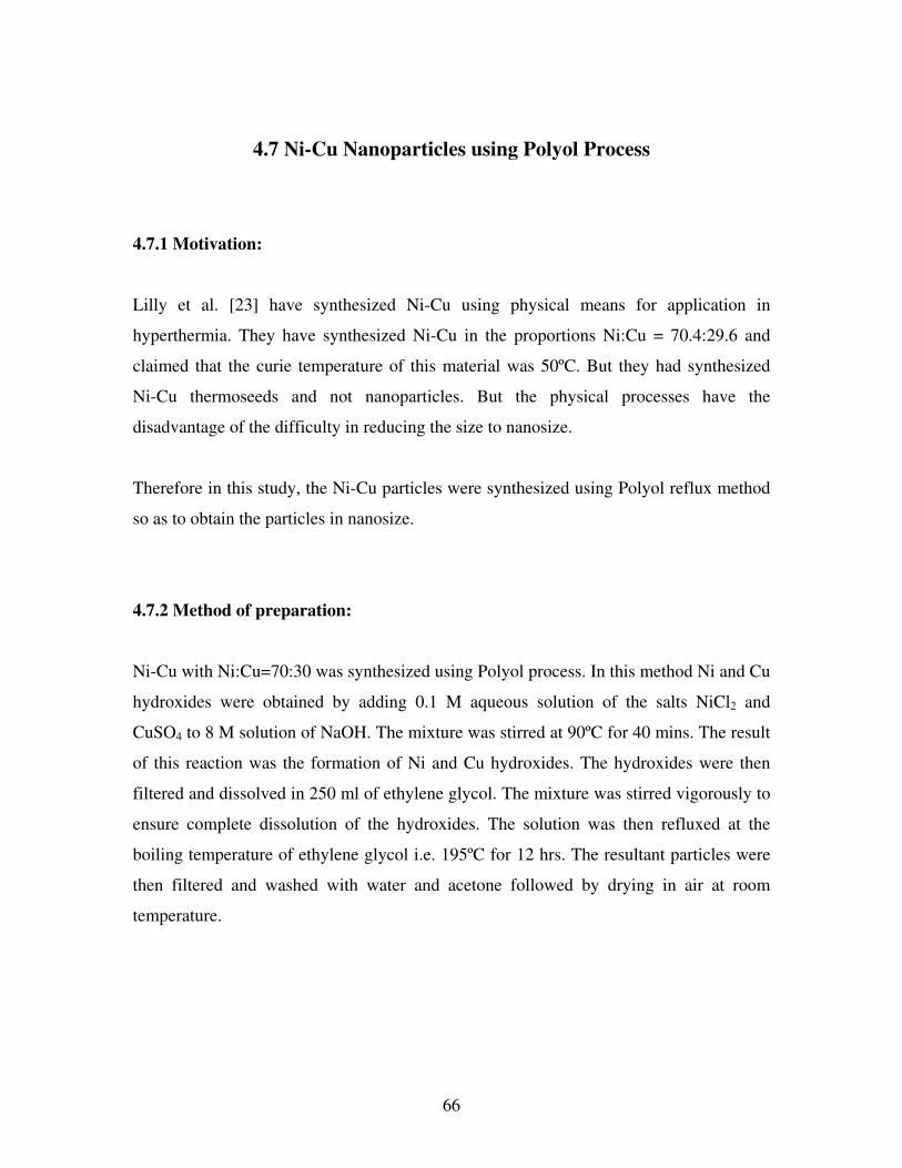
66
4.7 Ni-Cu Nanoparticles using Polyol Process
4.7.1 Motivation:
Lilly et al. [23] have synthesized Ni-Cu using physical means for application in
hyperthermia. They have synthesized Ni-Cu in the proportions Ni:Cu = 70.4:29.6 and
claimed that the curie temperature of this material was 50ºC. But they had synthesized
Ni-Cu thermoseeds and not nanoparticles. But the physical processes have the
disadvantage of the difficulty in reducing the size to nanosize.
Therefore in this study, the Ni-Cu particles were synthesized using Polyol reflux method
so as to obtain the particles in nanosize.
4.7.2 Method of preparation:
Ni-Cu with Ni:Cu=70:30 was synthesized using Polyol process. In this method Ni and Cu
hydroxides were obtained by adding 0.1 M aqueous solution of the salts NiCl2 and
CuSO4 to 8 M solution of NaOH. The mixture was stirred at 90ºC for 40 mins. The result
of this reaction was the formation of Ni and Cu hydroxides. The hydroxides were then
filtered and dissolved in 250 ml of ethylene glycol. The mixture was stirred vigorously to
ensure complete dissolution of the hydroxides. The solution was then refluxed at the
boiling temperature of ethylene glycol i.e. 195ºC for 12 hrs. The resultant particles were
then filtered and washed with water and acetone followed by drying in air at room
temperature.

67
4.7.3 Characterization results:
The characterization results of this sample are presented below:
Figure 4-21 Temperature dependence of magnetization for Ni-Cu with Ni:Cu=70:30

68
Figure 4-22 Morphology of Ni-Cu particles with Ni:Cu=70:30 under TEM

69
4.7.4 Discussion of results:
It was observed that the curie temperature of the Ni-Cu nanoparticles synthesized using
Polyol process was far beyond what was claimed by Lilly et al. [23]. The reason for this
might be that Lilly et al. [23] had used physical means to synthesize the Ni-Cu and also
they had used thermoseeds and not nanoparticles. The magnetic properties differ largely
when the same material is in macroscopic form and when it is in nanosize.
The Curie temperature of the Ni-Cu nanoparticles synthesized was beyond the measuring
range of SQUID but was much above the desired 315 K. The Ni-Cu synthesized using
Polyol process was hence unfit for application in Hyperthermia using magnetic
nanoparticles.
Fig. 4.22 shows the Ni-Cu nanoparticles for Ni:Cu = 70:30 under a TEM. The average
particle size is observed to be 50 nm. The particles prepared by this method are well
separated i.e. they do not tend to agglomerate because the ethylene glycol acts as a
surfactant. It can be seen from Fig. 4.22 that the particles have an approximate spherical
shape and are well separated from each other.
4.8 Gd4C Nanoparticles
4.8.1 Motivation:
Gschneidner Jr. et al. [38] have synthesized various GdC alloys with different constituent
proportions using physical means (melting). They observed that for proportions of Gd
from 75% to 95% the Curie temperature was in the range 294 K to 350 K.

70
In this study a Gd-C alloy in the proportions Gd:C = 80:20 i.e. Gd4C was synthesized
using physical means since it was expected that this proportion will give an alloy with the
desired 315 K Curie temperature.
4.8.2 Method of preparation:
The Gd-C alloy in the proportions Gd:C = 80:20 i.e. Gd4C was synthesized by melting
the constituents in a high temperature arc furnace. The constituents were melted 4 times,
turning over the sample after each melt. The resulting chunk of alloy was broken down
into smaller size first using pliers and then ground using pestle. Finally the ground alloy
was reduced to nanosize using an ultrasonicator.
.
4.8.3 Characterization results:
The characteristics of this sample are presented below:
Figure 4-23 Temperature dependence of magnetization for Gd4C

71
4.8.4 Discussion of results:
The Curie temperature of the synthesized Gd4C was measured to be 298 K which is
below the desired 315 K. The results do not match with those of Gschneidner Jr. et al.
[38]. The reason for this non-conformity might be the fact that Gschneidner Jr. et al. [38]
had tested the Curie temperature of the bulk alloy; whereas in this study the size was
reduced down to nanosize due do which their properties change as compared to that of
the bulk alloy. Also reducing the alloy to nanosize makes the alloy more susceptible to
oxidation due to the increase in the surface to volume ratio which might have resulted in
the Curie temperature being lower than expected.

72
CHAPTER 5
ENCAPSULATION OF MAGNETIC NANOPARTICLES
AND THEIR TESTING
Magnetic nanoparticles for the hyperthermia application have to be injected locally or
intravenously at the site of the tumor. Unfortunately, the inorganic magnetic
nanoparticles are not biocompatible. They are recognized by the phagocytic cells as
foreign products and are quickly removed from blood circulation. Essentially,
macrophages located in the reticoendothelial system (RES) play a crucial role to
phagocytize injected particles. It is generally assumed that the rapid particle phagocytosis
is mediated by the adsorption of certain blood components (opsonins) onto the surface of
particles [39].
A solution to this problem is to encapsulate the magnetic nanoparticles in a polymeric or
protein shell. The polymer/protein should be such that it should avoid detection by the
RES and thus ensure longer sustenance of the particles within the body. Various studies
have been conducted to select a polymer or protein which is biocompatible. For example
polyethylene glycol (PEG) has been used to form microspheres for injecting into the
body [39, 40]. Also, polyvinyl alcohol has been used to form a protective coating over
the nanoparticles [41]. Also PLA-PEG (poly lactic acid – polyethylene glycol) and PLA-
PEG-PLA polymers have been used for forming the shells [42, 43]. Use of PLGA (poly
lactic glycolide) as a coating material has also been reported [44]. A protein - human
serum albumin (HSA) has also been used for coating magnetic nanoparticles [45].
The encapsulated magnetic nanoparticles were then tested for effectiveness of heating
and for the breakage of polymer/protein at elevated temperatures

73
5.1 Methods for Preparation of Polymer/Protein Coatings
The nanoparticles are coated using polymer/proteins by forming nano or micro spheres in
a suspension containing magnetic nanoparticles. When the nano/micro spheres are
formed the magnetic particles are trapped inside these spheres thus encapsulating them.
Polymer microparticles (MPs) and nanoparticles belong to the class of multiphase
systems in which one or more microphases are dispersed in a continuous matrix of
different composition or physical state. The main characteristic of colloidal dispersions is
their extremely large interface area between the dispersed phase and the continuous
phase. Colloidal dispersions are metastable or unstable, since minimization of interface
free energy between two different phases is dictated by thermodynamic constraints.
However, in some cases colloids display significant kinetic stability that prevents their
aggregation. Hence, production of MPs and NPs relies essentially upon the chemical
production of colloidal dispersions, their kinetic stabilization, and effective recovery of
the final formulates. Polymeric materials are constituted by large molecules whose
peculiar solution characteristics often allow for the preparation of stable and size-
controlled colloidal dispersions, which in turn can be converted into MPs and NPs. In
addition, several polymers can be used as stabilizers of colloidal dispersions, since they
provide a surface coating of the metastable microphase, thus lowering its tendency to
phase-aggregation. The common feature of all methods for the preparation of MPs and
NPs is the externally-induced separation of at least two phases. This process is better
known as coacervation, and it may be promoted by a number of different techniques.
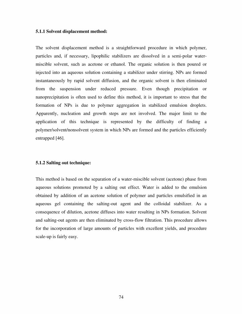
74
5.1.1 Solvent displacement method:
The solvent displacement method is a straightforward procedure in which polymer,
particles and, if necessary, lipophilic stabilizers are dissolved in a semi-polar water-
miscible solvent, such as acetone or ethanol. The organic solution is then poured or
injected into an aqueous solution containing a stabilizer under stirring. NPs are formed
instantaneously by rapid solvent diffusion, and the organic solvent is then eliminated
from the suspension under reduced pressure. Even though precipitation or
nanoprecipitation is often used to define this method, it is important to stress that the
formation of NPs is due to polymer aggregation in stabilized emulsion droplets.
Apparently, nucleation and growth steps are not involved. The major limit to the
application of this technique is represented by the difficulty of finding a
polymer/solvent/nonsolvent system in which NPs are formed and the particles efficiently
entrapped [46].
5.1.2 Salting out technique:
This method is based on the separation of a water-miscible solvent (acetone) phase from
aqueous solutions promoted by a salting out effect. Water is added to the emulsion
obtained by addition of an acetone solution of polymer and particles emulsified in an
aqueous gel containing the salting-out agent and the colloidal stabilizer. As a
consequence of dilution, acetone diffuses into water resulting in NPs formation. Solvent
and salting-out agents are then eliminated by cross-flow filtration. This procedure allows
for the incorporation of large amounts of particles with excellent yields, and procedure
scale-up is fairly easy.

75
5.1.3 Emulsion diffusion method:
The emulsion diffusion method is a slight modification of the salting-out technique. It
differs mainly because the organic solvent is only partially miscible with water, and it is
previously saturated with water, in order to reach an initial thermodynamic equilibrium
between water and the organic phase. After addition of water, solvent diffusion is
observed, and a nanoparticle suspension is formed.
5.1.4 Solvent evaporation method:
The solvent evaporation method is a well known technique [42, 43] that basically consists
in the formation of a bi- (o/w) or tri-phase emulsion (w/o/w). The inner phase is
constituted by a polymer solution in organic solvent in the biphase procedure, and a water
in oil emulsion in triphase method. In both cases, the continuous phase is an aqueous
solution in which the polymer is insoluble. The resulting emulsion is then exposed to a
high-energy mixer, such as ultrasonic devices, homogenizers, colloid mills, and
microfluidizers to reduce the globule size. Removal of the organic solvent by heat,
vacuum, or both results in the formation of a fine aqueous dispersion of NPs, which can
be collected and purified. This method is widely used for the preparation of micro and
nanoparticles made of polysaccharides, aliphatic polyesters, such as PLA, PLGA, PGA,
and other synthetic polymers such as PEG copolymers. The solvent evaporation method
may present some drawbacks. In fact, toxic chlorinated solvents, such as chloroform and
methylene chloride are often used because of their water insolubility, easy emulsification,
solubilizing properties, low boiling point. Moreover, the evaporation step can result in the
agglomeration of microparticles. The HSA coated nanoparticles were prepared using a
modified version of this method by chemical crosslinking.

76
5.1.5 Polymer emulsion process:
The polymer emulsification process patented by Vanderhoff et al. [47] is a modification
of the solvent evaporation method. This process comprises of intimately dispersing a
liquefied polymer phase in an aqueous liquid medium phase containing at least one
nonionic, anionic or cationic oil-in-water functioning emulsifying agent, in the presence
of a compound selected from the group consisting of those hydrocarbons and hydrocarbyl
alcohols, ethers, alcohol esters, amines, halides and carboxylic terminal aliphatic
hydrocarbyl group of atleast 8 carbon atoms, and mixtures thereof, and subjecting the
resulting crude emulsion to the action of comminuting forces sufficient to enable the
production of an aqueous emulsion containing polymer particles averaging less than
about 0.5 µm in size.
The solvent is preferably one which may be readily removed following the comminuting
step since in most instances an emulsion is desired which is devoid of organic solvents
posing problems of flammability, pollution, toxicity and/or odor ad the like. To remove
the solvent a vacuum evaporation technique is generally employed. The solvent should be
devoid of an aliphatic hydrocarbyl group of 8 or more carbon atoms, and inert in the
emulsion.
The oil-in-water functioning emulsifying agents employed in the process are generally
surface active agents also useful in the detergents field. The emulsifying agent is
operative in the aqueous medium in relatively low concentrations, being generally
included therein in proportions of about 0.1 to about 5%, preferably about 0.2 to about
3%, by weight of water in the aqueous phase.
The higher aliphatic hydrocarbyl-containing additive compound, or mixture thereof,
required in carrying out the process is generally employed in proportions of about 0.2 %
to about 12%, preferably about 0.4% to about 6%, by weight of the polymer phase. These
additives should be relatively highly water-insoluble. They should not have too high a
molecular weight e.g. not more than 5,000, preferable not more than about 2,000. Further

77
as a rule of thumb, when the additive is included in the aqueous phase, its weight ratio
relative to the emulsifying agent is generally more than 1:1 especially upto 4:1. When
included I the polymer phase, the ratio is about 0.3:1 to 1:1 I most cases. These additive
compounds increase the stability of these fine-sized particle emulsions by inhibiting
sedimentation or degradation caused by the tendency of the small particles or droplets to
coalesce molecularly. They should hence be inert, and resistant to diffusion into the
aqueous medium phase and to any solvent removal procedures applied after the
comminuting step.
In this process the polymer phase is admixed with stirring or other agitation into the
aqueous medium phase containing the emulsifying agent and the magnetic particles,
desirably at temperatures above room temperatures to below the boiling point of the
aqueous medium. It is desirable to produce emulsions with as high a solid content as
possible, and accordingly the ratio of the liquefied polymer phase to the aqueous medium
phase should be as high as possible without of course introducing inversion possibilities,
i.e. emulsification of the aqueous phase in the polymer phase. The weight ratio of the
polymer phase to the aqueous phase generally will range from about 0.2 to 1:1.
The resulting crude emulsion of coarse polymer phase droplets containing the magnetic
nanoparticles is then subjected to the action of comminuting forces sufficient to enable
the production of an aqueous emulsion containing polymer particles containing the
magnetic nanoparticles. An ultrasonicator was used in this study to supply this force.
The above described crude emulsion is passed through such comminuting device a
sufficient number of times, usually two, three or more times, until an emulsion is
obtained containing the desired small size polymer phase particles.
This is followed by the stripping or removal of the solvent from the emulsion e.g. by
vacuum evaporation technique.

78
In this study, the polymer emulsification process was used to synthesize PEG and Ethyl
cellulose coated magnetic nanoparticles.
5.2 Results and Discussions of Various Polymer/Protein Encapsulated
Particles Prepared in this Study
5.2.1 Polyvinyl Alcohol encapsulated Iron Oxide:
Commercial IronOxide nanoparticles were used for encapsulation within PVA. In this
method 250 mg of Ironoxide NP obtained from Nanophase technology corporation was
suspended in 40 ml distilled water. 2 gm PVA (MW:125,000) obtained from
Polysciences Inc. was then added to this suspension. The PVA is water soluble and hence
dissolves easily. This solution was then sonicated using an ultrasonicator at 50%
amplitude for 5 mins in an ice bath. After sonication the resulting solution was washed
repeatedly with acetone to remove the excess polymer. The encapsulated nanoparticles
were stored in acetone.
The morphology of these PVA encapsulated ironoxide particles is shown in Fig. 5.1. The
dark shaded regions (ironoxide) within the lightly shaded circle (PVA spheres) indicate
that the ironoxide nanoparticles were well encapsulated within the PVA shell. Also, the
empty circles are because of the excess amount of PVA as compared to the ironoxide
particles.

79
Figure 5-1 PVA encapsulated ironoxide nanoparticles under TEM
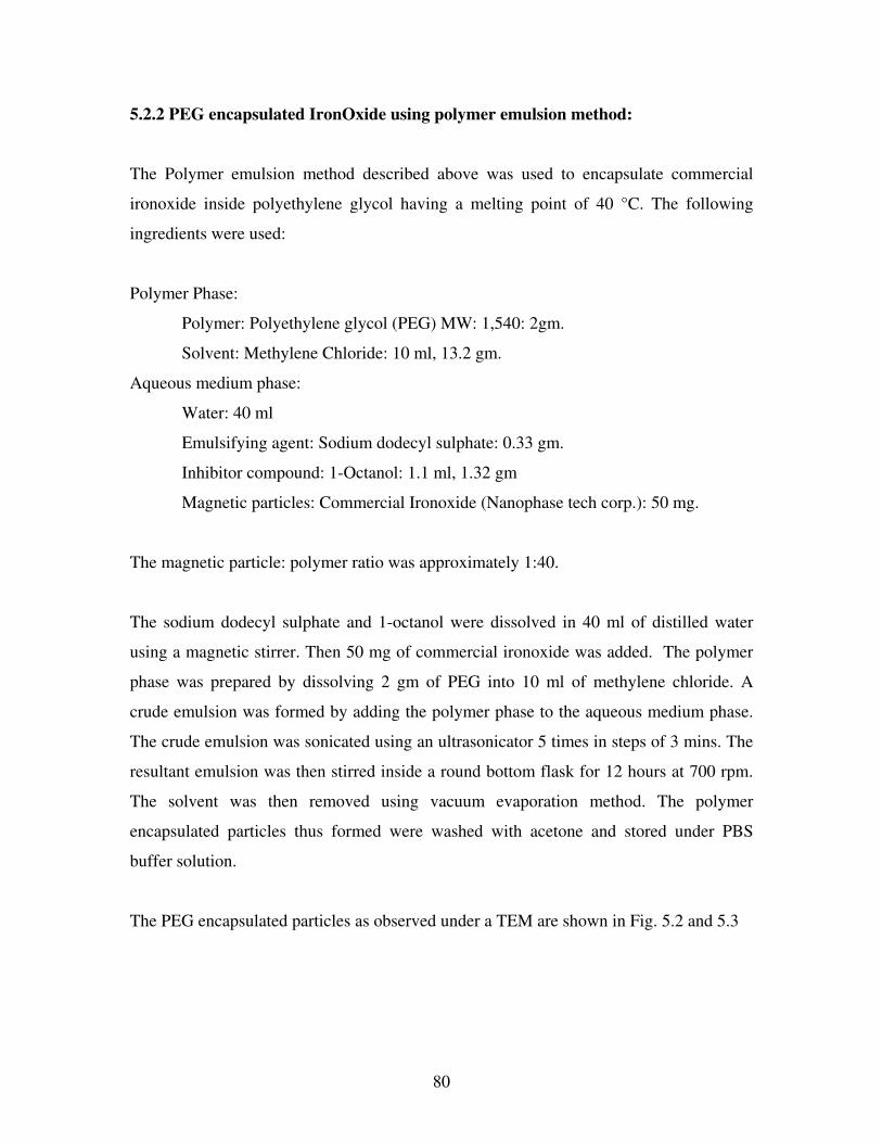
80
5.2.2 PEG encapsulated IronOxide using polymer emulsion method:
The Polymer emulsion method described above was used to encapsulate commercial
ironoxide inside polyethylene glycol having a melting point of 40 °C. The following
ingredients were used:
Polymer Phase:
Polymer: Polyethylene glycol (PEG) MW: 1,540: 2gm.
Solvent: Methylene Chloride: 10 ml, 13.2 gm.
Aqueous medium phase:
Water: 40 ml
Emulsifying agent: Sodium dodecyl sulphate: 0.33 gm.
Inhibitor compound: 1-Octanol: 1.1 ml, 1.32 gm
Magnetic particles: Commercial Ironoxide (Nanophase tech corp.): 50 mg.
The magnetic particle: polymer ratio was approximately 1:40.
The sodium dodecyl sulphate and 1-octanol were dissolved in 40 ml of distilled water
using a magnetic stirrer. Then 50 mg of commercial ironoxide was added. The polymer
phase was prepared by dissolving 2 gm of PEG into 10 ml of methylene chloride. A
crude emulsion was formed by adding the polymer phase to the aqueous medium phase.
The crude emulsion was sonicated using an ultrasonicator 5 times in steps of 3 mins. The
resultant emulsion was then stirred inside a round bottom flask for 12 hours at 700 rpm.
The solvent was then removed using vacuum evaporation method. The polymer
encapsulated particles thus formed were washed with acetone and stored under PBS
buffer solution.
The PEG encapsulated particles as observed under a TEM are shown in Fig. 5.2 and 5.3

81
Figure 5-2 PEG encapsulated ironoxide at low magnification under TEM
Fig. 5.2 shows the PEG encapsulated ironoxide nanoparticles under a TEM at low
magnification. The image shows PEG spheres of varying sizes from 20 nm to 200 nm.

82
Figure 5-3 PEG encapsulated ironoxide at high magnification under TEM

83
Figure 5-3 continued
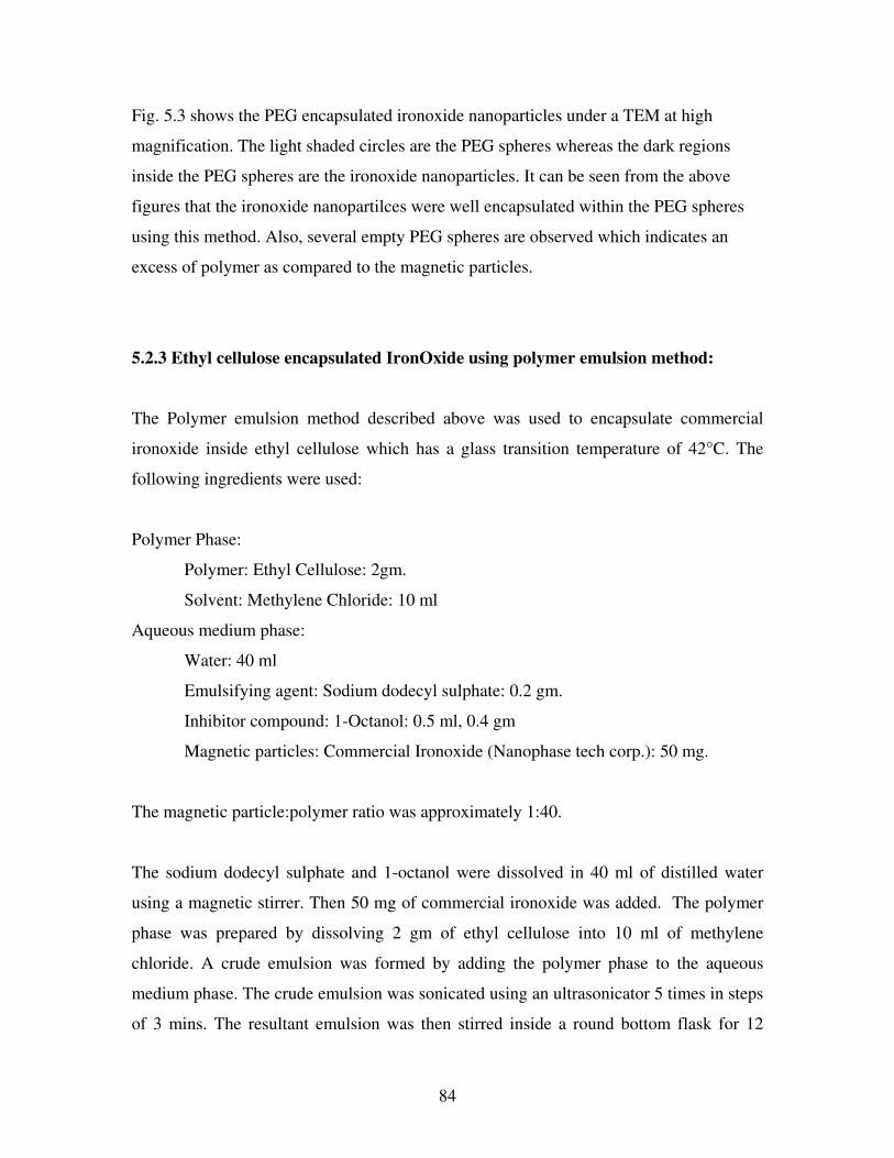
84
Fig. 5.3 shows the PEG encapsulated ironoxide nanoparticles under a TEM at high
magnification. The light shaded circles are the PEG spheres whereas the dark regions
inside the PEG spheres are the ironoxide nanoparticles. It can be seen from the above
figures that the ironoxide nanopartilces were well encapsulated within the PEG spheres
using this method. Also, several empty PEG spheres are observed which indicates an
excess of polymer as compared to the magnetic particles.
5.2.3 Ethyl cellulose encapsulated IronOxide using polymer emulsion method:
The Polymer emulsion method described above was used to encapsulate commercial
ironoxide inside ethyl cellulose which has a glass transition temperature of 42°C. The
following ingredients were used:
Polymer Phase:
Polymer: Ethyl Cellulose: 2gm.
Solvent: Methylene Chloride: 10 ml
Aqueous medium phase:
Water: 40 ml
Emulsifying agent: Sodium dodecyl sulphate: 0.2 gm.
Inhibitor compound: 1-Octanol: 0.5 ml, 0.4 gm
Magnetic particles: Commercial Ironoxide (Nanophase tech corp.): 50 mg.
The magnetic particle:polymer ratio was approximately 1:40.
The sodium dodecyl sulphate and 1-octanol were dissolved in 40 ml of distilled water
using a magnetic stirrer. Then 50 mg of commercial ironoxide was added. The polymer
phase was prepared by dissolving 2 gm of ethyl cellulose into 10 ml of methylene
chloride. A crude emulsion was formed by adding the polymer phase to the aqueous
medium phase. The crude emulsion was sonicated using an ultrasonicator 5 times in steps
of 3 mins. The resultant emulsion was then stirred inside a round bottom flask for 12

85
hours at 700 rpm. The solvent was then removed using vacuum evaporation method. The
polymer encapsulated particles thus formed were washed with acetone and stored under
PBS buffer solution.
Figure 5-4 Ethyl cellulose encapsulated iron oxide particles under TEM

86
Fig 5.4 shows the ethyl cellulose encapsulate ironoxide nanoparticles under a TEM. The
lightly shaded circles are the ethyl cellulose spheres whereas the dark shaded regions are
the ironoxide nanoparticles. As seen from the above figure the ironoxide nanoparticles
were found to be well encapsulated within ethyl cellulose spheres. Also, the empty ethyl
cellulose spheres indicate an excess of polymer as compared to the nanoparticles.
5.2.4 PEG encapsulated IronOxide by Glutaraldehyde crosslinking:
In this method 500 mg of commercial ironoxide was suspended in 40 ml methylene
chloride. 2 gm of PEG (MW: 125,000) was added to this suspension followed by
sonication for 5 mins at 50% amplitude. 10 ml Glutaraldehyde was then added as a
crosslinking agent and the resulting solution was stirred in a round bottom flask for 2 hrs.
The PEG coated nanoparticles were then washed with acetone and stored under PBS
buffer.
Figure 5-5 PEG encapsulated ironoxide particles prepared by glutaraldehyde crosslinking
method under TEM

87
The PEG encapsulated ironoxide particles prepared by this method as observed under a
TEM are shown in Fig. 5.5. The lightly shaded circles are the PEG spheres whereas the
dark regions are the ironoxide nanoparticles. The nanoparticles were found to be well
encapsulated using this method.
5.2.5 HSA encapsulated Gd-Zn-Ferrite nanoparticles:
Human serum albumin (HSA) is a single chain polypeptide of 585 residues, which
comprises about 60% of the plasma protein. In human, albumin is synthesized in the liver
and posses a half-life in circulation of 19-20 days [48]. Hence HAS can be used to
encapsulate the magnetic nanoparticles to ensure that they stay in the body for a longer
time and are not easily eliminated by the RES. The Gd-Zn-Ferrite with Gd = 0.02 which
was found to have a Curie temperature of 315 K in the results discussed earlier were
used.
The process used for the preparation of these particles was on the lines of the modified
suspension crosslinking method used by Chatterjee et al. [45]. The process consisted of
the following steps.
a) Preparation of glutaraldehyde saturated with toluene: 10 ml of 25%
glutaraldehyde and 10 ml. of toluene were dispersed ultrasonically at 50%
amplitude. The mixing was done in an ice-bath and in two five min steps.
Afterwards the mixture was taken in a separating funnel and the milky white
phase (GST) is separated. The phase separation process was repeated thrice by
adding 10 ml of toluene for each repetition to ensure complete separation.
b) Preparation of HSA – Gd-Zn-Ferrite particles in water: 250 mg. of HSA and
about 75 mg. of Gd-Zn-Ferrite were dissolved in 1 ml. of distilled water and this
mixture was added dropwise to a mixture of 40 ml. of n-hexane, 10 ml. of light

88
mineral oil (LMO) and 0.5 ml. of sorbitan sesquioleate. This inverse (water-in-oil)
emulsion is sonicated for three times (5 min each) at 50% amplitude. The
ultrasonication is carried out in an ice-water bath to prevent heat denaturation of
albumin protein.
c) Crosslinking of HSA micro/nano spheres with glutaraldehyde: The above
dispersion is then mixed with 10 ml. of GST and the mixture is stirred at 1500
rpm for 2 hrs using a motor operated Teflon coated stirrer. The micro/nano
spheres thus formed are centrifuged and washed with petroleum ether repeatedly
followed by washing with PBS and stored in acetone.
The morphology of the HSA encapsulated Gd-Zn-Ferrite, Gd = 0.02 is shown in Fig. 5.6,
5.7 and 5.8
Figure 5-6 HSA encapsulated Gd-Zn-Ferrite, Gd=0.02 under TEM at high magnification

89
Figure 5-7 HSA encapsulated Gd-Zn-Ferrite, Gd=0.02 under TEM at high magnification

90
Figure 5-8 HSA encapsulated Gd-Zn-Ferrite, Gd=0.02 under TEM at low magnification
The above figures show that the magnetic nanoparticles were well encapsulated within
HAS using this method. Also, it was observed that each HSA shell encapsulated on an
average one magnetic particle. The empty light shaded circles indicate the excess HSA
compared to the amount of magnetic particles.
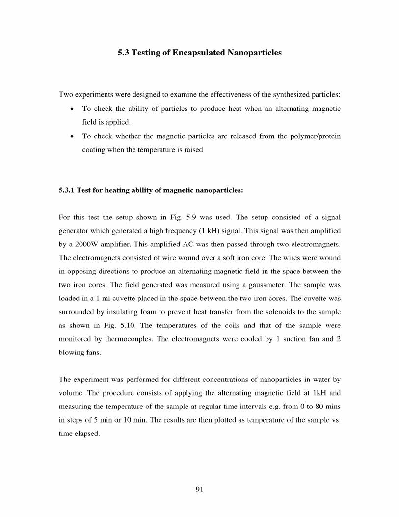
91
5.3 Testing of Encapsulated Nanoparticles
Two experiments were designed to examine the effectiveness of the synthesized particles:
• To check the ability of particles to produce heat when an alternating magnetic
field is applied.
• To check whether the magnetic particles are released from the polymer/protein
coating when the temperature is raised
5.3.1 Test for heating ability of magnetic nanoparticles:
For this test the setup shown in Fig. 5.9 was used. The setup consisted of a signal
generator which generated a high frequency (1 kH) signal. This signal was then amplified
by a 2000W amplifier. This amplified AC was then passed through two electromagnets.
The electromagnets consisted of wire wound over a soft iron core. The wires were wound
in opposing directions to produce an alternating magnetic field in the space between the
two iron cores. The field generated was measured using a gaussmeter. The sample was
loaded in a 1 ml cuvette placed in the space between the two iron cores. The cuvette was
surrounded by insulating foam to prevent heat transfer from the solenoids to the sample
as shown in Fig. 5.10. The temperatures of the coils and that of the sample were
monitored by thermocouples. The electromagnets were cooled by 1 suction fan and 2
blowing fans.
The experiment was performed for different concentrations of nanoparticles in water by
volume. The procedure consists of applying the alternating magnetic field at 1kH and
measuring the temperature of the sample at regular time intervals e.g. from 0 to 80 mins
in steps of 5 min or 10 min. The results are then plotted as temperature of the sample vs.
time elapsed.

92
Figure 5-9 Setup for testing the heating ability of magnetic nanoparticles
Fig. 5.11 shows the results for this experiment for the Gd-Zn Ferrite with Gd = 0.02
nanoparticle sample. It was observed that the magnetic nanoparticles were heated to a
temperature of approximately 47°C under the influence of the alternating magnetic field
at a sample concentration of 70% with water by volume. The Curie temperature for this
sample as determined from the SQUID analysis was 315 K (42°C). But in this test the
samples were heated upto 47°C and the temperature remained constant thereafter.

93
Figure 5-10 Electromagnet setup showing position of sample in cuvette

94
Figure 5-11 Results of test for heating ability of Gd-Zn Ferrite with Gd = 0.02 sample
The test results for the same sample (Gd-Zn Ferrite, Gd = 0.02) encapsulated within HSA
are shown in Fig. 5.12. The graph shows that under the action of the alternating B-field,
the particles were heated upto 48°C and the temperature remained constant thereafter.
Gd-Zn Ferrite, Gd=0.02, Tc=42 C
0
5
10
15
20
25
30
35
40
45
50
0 5 10 15 20 25 30 35 40 45 50 Time (min)
Temp (C)
50%
60%
70%
40%

95
HSA encapsulated Gd-Zn Ferrite, Gd = 0.02 NP
0
5
10
15
20
25
30
35
40
45
0 10 20 30 40 50 60 70 80 90Time (min)
Te
mp
(C
)
50%
80%
Figure 5-12 Results of test for heating ability of HAS encapsulated Gd-Zn Ferrite,
Gd=0.02 particles
5.3.1 Test for polymer/protein breakage at elevated temperatures:
For this test, 1 ml of particle suspension was added to about 15 ml. distilled water in a
beaker. This beaker was then heated gradually using a heating plate. The temperature of
the solution was monitored continuously using a mercury thermometer. If the polymer is
broken it will be detached from the encapsulated magnetic particles and will float in the
suspension. So if a magnetic field is applied at the bottom of the beaker using a magnet
all the magnetic nanoparticles will settle down and the broken polymer fragments will
float in the suspension. Thus if any such fragments are observed in the suspension after
heating till a certain temperature it can be safely assumed that the polymer was broken at
this temperature thus releasing the encapsulated magnetic particles.

96
When the above mentioned test was conducted on the PEG encapsulated ironoxide
nanoparticles, a few fragments of non-magnetic material was found floating on the
surface of the suspension when heated upto 45°C. Since care was taken to prevent any
kind of dust or impurity contamination it can be assumed that the floating fragments were
those of the PEG. Thus it was observed that the PEG coating was broken at about 45°C.
The melting point of the PEG used was 40°C. The rise in this melting point may be
attributed to the crosslinking of the polymer.

97
CHAPTER 6
CONCLUSIONS AND RECOMMENDATIONS
This chapter derives conclusions from the study carried out and suggests
recommendations for future work.
6.1 Conclusions
The aim of this study was to find out a material for magnetic nanoparticles which will
have properties suitable for use in self-controlled hyperthermia:
• Curie temperature of 42ºC (315 K)
• A high pyromagnetic co-efficient
• Made up of bio-compatible elements
To achieve these goals various magnetic nanoparticles were synthesized using both
physical and mostly chemical means. All the particles were characterized to check
whether they meet the above stated requirements. For most of the particles, numerous
samples were made by varying the constituent proportions to study the effect on their
properties. Accordingly, various trends were observed in the properties for which reasons
were sought using solid state physics. The Details of a selected few samples amongst
these, have been presented in Table 6.1.
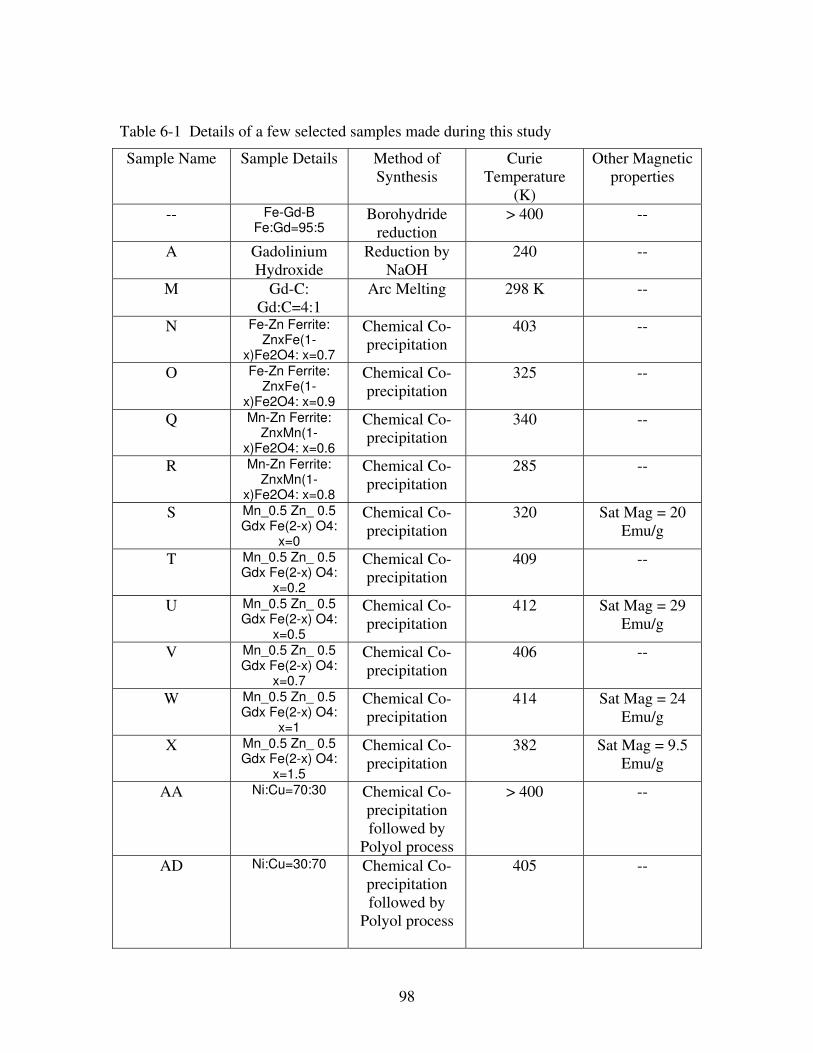
98
Table 6-1 Details of a few selected samples made during this study
Sample Name Sample Details Method of
Synthesis
Curie
Temperature
(K)
Other Magnetic
properties
-- Fe-Gd-B Fe:Gd=95:5
Borohydride
reduction
> 400 --
A Gadolinium
Hydroxide
Reduction by
NaOH
240 --
M Gd-C:
Gd:C=4:1
Arc Melting 298 K --
N Fe-Zn Ferrite: ZnxFe(1-
x)Fe2O4: x=0.7
Chemical Co-
precipitation
403 --
O Fe-Zn Ferrite: ZnxFe(1-
x)Fe2O4: x=0.9
Chemical Co-
precipitation
325 --
Q Mn-Zn Ferrite: ZnxMn(1-
x)Fe2O4: x=0.6
Chemical Co-
precipitation
340 --
R Mn-Zn Ferrite: ZnxMn(1-
x)Fe2O4: x=0.8
Chemical Co-
precipitation
285 --
S Mn_0.5 Zn_ 0.5 Gdx Fe(2-x) O4:
x=0
Chemical Co-
precipitation
320 Sat Mag = 20
Emu/g
T Mn_0.5 Zn_ 0.5 Gdx Fe(2-x) O4:
x=0.2
Chemical Co-
precipitation
409 --
U Mn_0.5 Zn_ 0.5 Gdx Fe(2-x) O4:
x=0.5
Chemical Co-
precipitation
412 Sat Mag = 29
Emu/g
V Mn_0.5 Zn_ 0.5 Gdx Fe(2-x) O4:
x=0.7
Chemical Co-
precipitation
406 --
W Mn_0.5 Zn_ 0.5 Gdx Fe(2-x) O4:
x=1
Chemical Co-
precipitation
414 Sat Mag = 24
Emu/g
X Mn_0.5 Zn_ 0.5 Gdx Fe(2-x) O4:
x=1.5
Chemical Co-
precipitation
382 Sat Mag = 9.5
Emu/g
AA Ni:Cu=70:30 Chemical Co-
precipitation
followed by
Polyol process
> 400 --
AD Ni:Cu=30:70 Chemical Co-
precipitation
followed by
Polyol process
405 --

99
Table 6-1 Continued
Sample Name Sample Details Method of
Synthesis
Curie
Temperature
(K)
Other Magnetic
properties
AE Zn Ferrite Chemical Co-
precipitation
345 --
AF Gd subs Zn Ferrite: ZnO.Gdx Fe(2-x) O3: x =
0.4
Chemical Co-
precipitation
> 400 --
AG Gd subs Zn Ferrite: ZnO.Gdx Fe(2-x) O3: x =
0.8
Chemical Co-
precipitation
> 400 --
AI Gd subs Zn Ferrite: ZnO.Gdx Fe(2-x) O3: x =
0.1
Chemical Co-
precipitation
> 400 --
AJ Zn Ferrite Chemical Co-
precipitation
followed by
quenching
240 --
AK Gd subs Zn Ferrite: ZnO.Gdx Fe(2-x) O3: x =
0.1
Chemical Co-
precipitation
followed by
quenching
370 --
AL Gd subs Zn Ferrite: ZnO.Gdx Fe(2-x) O3: x =
0.02
Chemical Co-
precipitation
followed by
quenching
315 --
AM Gd subs Zn Ferrite: ZnO.Gdx Fe(2-x) O3: x =
0.05
Chemical Co-
precipitation
followed by
quenching
350 --
The magnetic saturation was determined for only a few of the samples synthesized
because the focus of this study was on obtaining the desired Curie temperature.
Therefore, the magnetic saturation, coercivity and retentivity fields for most of the
samples in Table 6.1 are empty.
Amongst the various particles synthesized the Gd substituted Zn Ferrite nanoparticles
with Gd proportion, x = 0.02 were found to possess these desired qualities. They had a

100
Curie temperature of 315 K and a high pyromagnetic co-efficient. Besides, all the
constituent elements Gd, Fe, Zn and O are found in the human body in small or large
quantities.
Also, in this study a curve representing the relation between Curie temperature and Gd
proportion was obtained which makes it possible to fine tune the Curie temperature of the
particles as per the need. As a result the particles can now be tested in vitro and in vivo
followed by necessary manipulations in the Gd proportion to zero in on the composition
which will give a Curie temperature of 315 K and hence can be used for the hyperthermia
application.
It is imperative that these nanoparticles be encapsulated within biocompatible
polymers/proteins to avoid quick elimination by the reticoendothelial system (RES).
Various polymers and proteins were used to encapsulate commercial IronOxide
nanopowder as well as Gd-Zn-Ferrite nanoparticles with Gd = 0.02. PEG with MW:
125,000 which has a melting point of 40°C is especially important because if the
magnetic nanoparticles are encapsulated inside PEG, when their temperature reaches
42°C the PEG coating will lyse open thus releasing the nanoparticles. Also, HSA which
has a half-life circulation time of 19-20 days is significant because if the magnetic
nanoparticles are encapsulated inside HSA then they can sustain inside the body for a
long time. The TEM images of these encapsulated magnetic particles show that the
magnetic nanoparticles are well encapsulated within the polymer/protein and hence can
be used to inject inside the human body.
6.2 Recommendations for future work
In addition to encapsulating the magnetic particles in the polymers/proteins a suitable
drug can also be included. By this method it is possible to effect targeted drug delivery.
The drug to be delivered may be a chemotherapy drug or a radiosensitizer. There are
many possibilities for the drug which can be used in this technique.

101
An effective and reliable method of determining the Curie temperature is necessary. The
setup to apply the alternating magnetic field can be improvised to provide fields of even
higher frequencies.
Also, the search for heat sensitive polymer/protein with melting point of 42°C can be
extended to find novel materials. An accurate method for testing of the polymer breakage
and subsequent particle release at elevated temperatures is also necessary.

102
APPENDIX A
This appendix gives general information about cancer, their possible causes, diagnosis,
symptoms and different types of cancer. All the information in this appendix including
the figures has been gathered from www.cancer.gov [1]. This appendix serves as an
abridged version of the information given on this web-site.
A.1 Possible causes and prevention of cancer
In the laboratory, scientists explore possible causes of cancer and try to determine exactly
what happens in cells when they become cancerous. Researchers also study patterns of
cancer in the population to look for risk factors, conditions that increase the chance that
cancer might occur. They also look for protective factors, things that decrease the risk.
Even though doctors can seldom explain why one person gets cancer and another does
not, it is clear that cancer is not caused by an injury, such as a bump or bruise. And
although being infected with certain viruses may increase the risk of some types of
cancer, cancer is not contagious; no one can "catch" cancer from another person.
Cancer develops over time. It is a result of a complex mix of factors related to lifestyle,
heredity, and environment. A number of factors that increase a person's chance of
developing cancer have been identified. Many types of cancer are related to the use of
tobacco, what people eat and drink, exposure to ultraviolet (UV) radiation from the sun,
and, to a lesser extent, exposure to cancer-causing agents (carcinogens) in the

103
environment and the workplace. Some people are more sensitive than others to factors
that can cause cancer.
Still, most people who get cancer have none of the known risk factors. And most people
who do have risk factors do not get the disease.
Some cancer risk factors can be avoided. Others, such as inherited factors, are
unavoidable, but it may be helpful to be aware of them.
These are some of the factors that increase the likelihood of cancer:
• Tobacco: Smoking tobacco, using smokeless tobacco, and being regularly
exposed to environmental tobacco smoke are responsible for one-third of all
cancer deaths in the United States each year. Tobacco use is the most preventable
cause of death in this country. Smoking accounts for more than 85 percent of all
lung cancer deaths. People who smoke cigars or pipes have a risk for cancers of
the oral cavity that is similar to the risk for people who smoke cigarettes. Cigar
smokers also have an increased chance of developing cancers of the lung, larynx,
esophagus, and pancreas. Studies suggest that exposure to environmental tobacco
smoke, also called secondhand smoke, increases the risk of lung cancer for
nonsmokers.
• Diet. Researchers are exploring how dietary factors play a role in the
development of cancer. Some evidence suggests a link between a high-fat diet and
certain cancers, such as cancers of the colon, uterus, and prostate. Being seriously
overweight may be linked to breast cancer among older women and to cancers of
the prostate, pancreas, uterus, colon, and ovary. On the other hand, some studies
suggest that foods containing fiber and certain nutrients may help protect against
some types of cancer.
• Ultraviolet (UV) radiation. UV radiation from the sun causes premature aging of
the skin and skin damage that can lead to skin cancer. Artificial sources of UV

104
radiation, such as sunlamps and tanning booths, also can cause skin damage and
probably an increased risk of skin cancer.
• Alcohol. Heavy drinkers have an increased risk of cancers of the mouth, throat,
esophagus, larynx, and liver. (People who smoke cigarettes and drink heavily
have an especially high risk of getting these cancers.) Some studies suggest that
even moderate drinking may slightly increase the risk of breast cancer.
• Ionizing radiation. Cells may be damaged by ionizing radiation from x-ray
procedures, radioactive substances, rays that enter the Earth's atmosphere from
outer space, and other sources. In very high doses, ionizing radiation may cause
cancer and other diseases. Studies of survivors of the atomic bomb in Japan show
that ionizing radiation increases the risk of developing leukemia and cancers of
the breast, thyroid, lung, stomach, and other organs.
• Chemicals and other substances. Being exposed to substances such as certain
chemicals, metals, or pesticides can increase the risk of cancer. Asbestos, nickel,
cadmium, uranium, radon, vinyl chloride, benzidene, and benzene are examples
of well-known carcinogens.
• Hormone replacement therapy 1(HRT). Doctors may recommend HRT, using
either estrogen2 alone or estrogen in combination with progesterone
3, to control
symptoms (such as hot flashes and vaginal dryness) that may occur during
menopause. Studies have shown that the use of estrogen alone increases the risk
of cancer of the uterus.
• Diethylstilbestrol (DES). DES is a synthetic form of estrogen that was used
between the early 1940s and 1971. Some women took DES during pregnancy to
prevent certain complications. Their DES-exposed daughters have an increased
1 HRT. Hormones (est rogen, progesterone, or both) given to women after menopause to replace
the hormones no longer produced by the ovaries. Also called menopausal hormone therapy.
2 A hormone that promotes the development and maintenance of female sex characterist ics.
3 A female hormone.

105
chance of developing abnormal cells (dysplasia4) in the cervix and vagina. In
addition, a rare type of vaginal and cervical cancer can occur in DES-exposed
daughters. Women who took DES during pregnancy may have a slightly higher
risk for developing breast cancer.
• Close relatives with certain types of cancer. Some types of cancer (including
melanoma and cancers of the breast, ovary, prostate, and colon) tend to occur
more often in some families than in the rest of the population. It is often unclear
whether a pattern of cancer in a family is primarily due to heredity, factors in the
family's environment or lifestyle, or just a matter of chance.
Researchers have learned that cancer is caused by changes (called mutations or
alterations) in genes that control normal cell growth and cell death. Most cancer-causing
gene changes are the result of factors in lifestyle or the environment. However, some
alterations that may lead to cancer are inherited; that is, they are passed from parent to
child. But having such an inherited gene alteration does not mean that the person is
certain to develop cancer; it means that the risk of cancer is increased.
A.2 Screening and early detection
Sometimes, cancer can be found before the disease causes symptoms. Checking for
cancer (or for conditions that may lead to cancer) in a person who does not have any
symptoms of the disease is called screening.
In routine physical exams, the doctor looks for anything unusual and feels for any lumps
or growths. Specific screening tests, such as lab tests, x-rays, or other procedures, are
used routinely for only a few types of cancer.
4 Cells that look abnormal under a microscope but are not cancer.

106
• Breast. A screening mammogram is the best tool available to find breast cancer
before symptoms appear. A mammogram is a special kind of x-ray image of the
breasts. Breast cancer screening has been shown to reduce the risk of dying from
this disease.
• Cervix. Doctors use the Pap test, or Pap smear, to screen for cancer of the cervix.
For this test, cells are collected from the cervix. The cells are examined under a
microscope to detect cancer or changes that may lead to cancer.
• Colon and rectum. A number of screening tests are used to find colon and rectal
(colorectal) cancer. Sometimes tumors in the colon or rectum can bleed. The fecal
occult blood test checks for small amounts of blood in the stool. The doctor
sometimes uses a thin, lighted tube called a sigmoidoscope to examine the rectum
and lower colon. Or, to examine the entire colon and rectum, a lighted instrument
called a colonoscope is used. If abnormal areas are seen, tissue can be removed
and examined under a microscope.
Although it is not certain that screening for other cancers actually saves lives, doctors
also may suggest screening for cancers of the skin, lung, and oral cavity. And doctors
may offer to screen men for prostate or testicular cancer, and women for ovarian cancer.
Doctors consider many factors before recommending a screening test. They weigh factors
related to the individual, the test, and the cancer that the test is intended to detect. For
example, doctors take into account the person's age, medical history and general health,
family history, and lifestyle. The doctor pays special attention to a person's risk for
developing specific types of cancer. In addition, the doctor will assess the accuracy and
the risks of the screening test and any follow-up tests that may be necessary. Doctors also
consider the effectiveness and side effects of the treatment that will be needed if cancer is
found.

107
A.3 Symptoms of cancer
Cancer can cause a variety of symptoms. These are some of them:
• Thickening or lump in the breast or any other part of the body
• Obvious change in a wart or mole
• A sore that does not heal
• Nagging cough or hoarseness
• Changes in bowel or bladder habits
• Indigestion or difficulty swallowing
• Unexplained changes in weight
• Unusual bleeding or discharge
When these or other symptoms occur, they are not always caused by cancer. They may
also be caused by infections, benign tumors, or other problems. Early cancer usually does
not cause pain.
A.4 Diagnosis
If symptoms are present, the doctor asks about the person's medical history and performs
a physical exam. In addition to checking general signs of health, the doctor may order
various tests and exams. These may include laboratory tests and imaging procedures. A
biopsy is usually necessary to determine whether cancer is present.

108
A.5 Types of Cancer
A.5.1 Bladder Cancer
Each year in the United States, bladder cancer is diagnosed in 38,000 men and 15,000
women. This is the fourth most common type of cancer in men and the eighth most
common in women.
The bladder is a hollow organ in the lower abdomen. It stores urine, the liquid waste
produced by the kidneys. Urine passes from each kidney into the bladder through a tube
called a ureter.
An outer layer of muscle surrounds the inner lining of the bladder. When the bladder is
full, the muscles in the bladder wall can tighten to allow urination. Urine leaves the
bladder through another tube, the urethra.
Figure A-1 Human Urinary Tract [1]

109
Cancer that is only in cells in the lining of the bladder is called superficial bladder cancer.
The doctor might call it carcinoma in situ. This type of bladder cancer often comes back
after treatment. If this happens, the disease most often recurs as another superficial cancer
in the bladder.
Cancer that begins as a superficial tumor may grow through the lining and into the
muscular wall of the bladder. This is known as invasive cancer. Invasive cancer may
extend through the bladder wall. It may grow into a nearby organ such as the uterus or
vagina (in women) or the prostate gland (in men). It also may invade the wall of the
abdomen.
When bladder cancer spreads outside the bladder, cancer cells are often found in nearby
lymph nodes. If the cancer has reached these nodes, cancer cells may have spread to other
lymph nodes or other organs, such as the lungs, liver, or bones.
A.5.2 Brain Tumor
The brain is a soft, spongy mass of tissue. It is protected by the bones of the skull and
three thin membranes called meninges. Watery fluid called cerebrospinal fluid cushions
the brain. This fluid flows through spaces between the meninges and through spaces
within the brain called ventricles.
A network of nerves carries messages back and forth between the brain and the rest of the
body. Some nerves go directly from the brain to the eyes, ears, and other parts of the
head. Other nerves run through the spinal cord to connect the brain with the other parts of
the body. Within the brain and spinal cord, glial cells surround nerve cells and hold them
in place.

110
Figure A-2 Longitudinal Section of the Human Brain [1]
Tumors that begin in brain tissue are known as primary tumors of the brain.
The most common primary brain tumors are gliomas. They begin in glial cells.
When cancer spreads from its original place to another part of the body, the new tumor
has the same kind of abnormal cells and the same name as the primary tumor. Cancer that
spreads to the brain from another part of the body is different from a primary brain tumor.
When cancer cells spread to the brain from another organ (such as the lung or breast),
doctors may call the tumor in the brain a secondary tumor or metastatic tumor. Secondary
tumors in the brain are far more common than primary brain tumors.
A.5.3 Breast Cancer
Breast cancer is the most common type of cancer among women in this country (other
than skin cancer). The number of new cases of breast cancer in women was estimated to
be about 212,600 in 2003.

111
The breasts are glands that can make milk. Each breast sits on chest muscles that cover
the ribs.
Each breast is divided into 15 to 20 sections called lobes. Lobes contain many smaller
lobules. Lobules contain groups of tiny glands that can produce milk. Milk flows from
the lobules through thin tubes called ducts to the nipple. The nipple is in the center of a
dark area of skin called the areola. Fat fills the spaces between the lobules and ducts.
The breasts also contain lymph vessels, which carry a clear fluid called lymph. The
lymph vessels lead to small, round organs called lymph nodes. Groups of lymph nodes
are found near the breast in the axilla (underarm), above the collarbone, in the chest
behind the breastbone, and in many other parts of the body. The lymph nodes trap
bacteria, cancer cells, or other harmful substances that may be in the lymphatic system.
Figure A-3 Anatomy of a Human female breast [1]

112
These pictures show the parts of the breast and the lymph nodes and lymph vessels near
the breast.
The stage is based on the size of the tumor and whether the cancer has spread. When
breast cancer spreads, cancer cells are often found in lymph nodes under the arm (axillary
lymph nodes).
A.5.4 Cancer of the Cervix
Each year, about 15,000 women in the United States learn that they have cancer of the
cervix.
The cervix is the lower, narrow part of the uterus (womb). The uterus, a hollow, pear-
shaped organ, is located in a woman's lower abdomen, between the bladder and the
rectum. The cervix forms a canal that opens into the vagina, which leads to the outside of
the body.
Figure A-4 Female reproductive system [1]
Cancer of the cervix also may be called cervical cancer. Like most cancers, it is named
for the part of the body in which it begins. Cancers of the cervix also are named for the

113
type of cell in which they begin. Most cervical cancers are squamous cell carcinomas.
Squamous cells are thin, flat cells that form the surface of the cervix.
A.5.5 Cancer of the Colon and Rectum
Together, cancers of the colon and rectum are among the most common cancers in the
United States. They occur in both men and women and are most often found among
people who are over the age of 50.
The colon and rectum are parts of the body's digestive system, which removes nutrients
from food and stores waste until it passes out of the body. Together, the colon and rectum
form a long, muscular tube called the large intestine (also called the large bowel). The
colon is the first 6 feet of the large intestine, and the rectum is the last 8 to 10 inches.
Figure A-5 Position of the colon [1]

114
Cancer that begins in the colon is called colon cancer, and cancer that begins in the
rectum is called rectal cancer. Cancers affecting either of these organs may also be called
colorectal cancer.
A.5.6 Cancer of the Esophagus
The esophagus is a hollow tube that carries food and liquids from the throat to the
stomach. When a person swallows, the muscular walls of the esophagus contract to push
food down into the stomach. Glands in the lining of the esophagus produce mucus, which
keeps the passageway moist and makes swallowing easier. The esophagus is located just
behind the trachea (windpipe). In an adult, the esophagus is about 10 inches long.
Figure A-6 The digestive system [1]
Cancer that begins in the esophagus (also called esophageal cancer) is divided into two
major types, squamous cell carcinoma and adenocarcinoma, depending on the type of
cells that are malignant. Squamous cell carcinomas arise in squamous cells that line the
esophagus. These cancers usually occur in the upper and middle part of the esophagus.

115
Adenocarcinomas usually develop in the glandular tissue in the lower part of the
esophagus. The treatment is similar for both types of esophageal cancer.
A.5.7 Kidney Cancer
Each year, more than 28,000 people in the United States learn that they have kidney
cancer.
The kidneys are two reddish-brown, bean-shaped organs located just above the waist, one
on each side of the spine. They are part of the urinary system. Their main function is to
filter blood and produce urine to rid the body of waste. As blood flows through the
kidneys, they remove waste products and unneeded water. The resulting liquid, urine,
collects in the middle of each kidney in an area called the renal pelvis. Urine drains from
each kidney through a long tube, the ureter, into the bladder, where it is stored. Urine
leaves the body through another tube, called the urethra.
The kidneys also produce substances that help control blood pressure and regulate the
formation of red blood cells.
Figure A-7 Urinary system [1]
116
Several types of cancer can develop in the kidney. Renal cell cancer is the most common
form of kidney cancer in adults. Transitional cell cancer (carcinoma), which affects the
renal pelvis, is a less common form of kidney cancer.
As kidney cancer grows, it may invade organs near the kidney, such as the liver, colon, or
pancreas. Kidney cancer cells may also break away from the original tumor and spread
(metastasize) to other parts of the body.
A.5.8 Cancer of the Larynx
Each year in the United States, more than 10,000 people learn they have this type of
cancer.
The larynx is an organ at the front of your neck. It is also called the voice box. It is about
2 inches long and 2 inches wide. It is above the windpipe (trachea). Below and behind the
larynx is the esophagus.
The larynx has two bands of muscle that form the vocal cords. The cartilage at the front
of the larynx is sometimes called the Adam’s apple.
The larynx has three main parts:
• The top part of the larynx is the supraglottis.
• The glottis is in the middle. Your vocal cords are in the glottis.
• The subglottis is at the bottom. The subglottis connects to the windpipe.

117
Figure A-8 The location and anatomy of Larynx [1]
Cancer of the larynx also may be called laryngeal cancer. It can develop in any part of the
larynx. Most cancers of the larynx begin in the glottis. The inner walls of the larynx are
lined with cells called squamous cells. Almost all laryngeal cancers begin in these cells.
These cancers are called squamous cell carcinomas.

118
If cancer of the larynx spreads (metastasizes), the cancer cells often spread to nearby
lymph nodes in the neck. The cancer cells can also spread to the back of the tongue, other
parts of the throat and neck, the lungs, and other parts of the body.
A.5.9 Leukemia:
Each year, leukemia is diagnosed in about 29,000 adults and 2,000 children in the United
States.
Blood cells form in the bone marrow. Bone marrow is the soft material in the center of
most bones.
Immature blood cells are called stem cells and blasts. Most blood cells mature in the bone
marrow and then move into the blood vessels. Blood flowing through the blood vessels
and heart is called the peripheral blood.
Figure A-9 The arising of cells from stem cell [1]

119
The bone marrow makes different types of blood cells. Each type has a special function:
• White blood cells help fight infection.
• Red blood cells carry oxygen to tissues throughout the body.
• Platelets help form blood clots that control bleeding.
In people with leukemia, the bone marrow produces abnormal white blood cells. The
abnormal cells are leukemia cells. At first, leukemia cells function almost normally. In
time, they may crowd out normal white blood cells, red blood cells, and platelets. This
makes it hard for blood to do its work.
The types of leukemia are grouped by how quickly the disease develops and gets worse.
Leukemia is either chronic (gets worse slowly) or acute (gets worse quickly).
The types of leukemia are also grouped by the type of white blood cell that is affected.
Leukemia can arise in lymphoid cells or myeloid cells. Leukemia that affects lymphoid
cells is called lymphocytic leukemia. Leukemia that affects myeloid cells is called
myeloid leukemia or myelogenous leukemia.
A.5.10 Lung Cancer
The lungs, a pair of sponge-like, cone-shaped organs, are part of the respiratory system.
The right lung has three sections, called lobes; it is a little larger than the left lung, which
has two lobes. When we breathe in, the lungs take in oxygen, which our cells need to live
and carry out their normal functions. When we breathe out, the lungs get rid of carbon
dioxide, which is a waste product of the body's cells.

120
Figure A-10 The anatomy of Lungs [1]
Cancers that begin in the lungs are divided into two major types, non-small cell lung
cancer and small cell lung cancer, depending on how the cells look under a microscope.
Each type of lung cancer grows and spreads in different ways and is treated differently.
Researchers have discovered several causes of lung cancer -- most are related to the use
of tobacco such as cigarettes, cigars, etc
A.5.11 Melanoma:
Each year in the United States, more than 53,600 people learn they have melanoma.
Melanoma is the most serious type of cancer of the skin. Each year in the United States,
more than 53,600 people learn they have melanoma.
Melanoma is a type of skin cancer. It begins in cells in the skin called melanocytes.

121
Melanocytes produce melanin, the pigment that gives skin its natural color. When skin is
exposed to the sun, melanocytes produce more pigment, causing the skin to tan, or
darken.
Figure A-11 The anatomy of the skin [1]
Melanoma occurs when melanocytes (pigment cells) become malignant. Most pigment
cells are in the skin; when melanoma starts in the skin, the disease is called cutaneous
melanoma.
When melanoma spreads, cancer cells may show up in nearby lymph nodes.
A.5.12 Oral Cancer
It includes the cancer of the oral cavity (mouth) and the oropharynx (the part of the throat
at the back of the mouth). The oral cavity includes many parts: the lips; the lining inside
the lips and cheeks, called the buccal mucosa; the teeth; the bottom (floor) of the mouth
under the tongue; the front two-thirds of the tongue; the bony top of the mouth (hard
palate); the gums; and the small area behind the wisdom teeth. The oropharynx includes
the back one-third of the tongue, the soft palate, the tonsils, and the part of the throat

122
behind the mouth. Salivary glands throughout the oral cavity make saliva, which keeps
the mouth moist and helps digest food.
Figure A-12 The anatomy of Human mouth cavity [1]
When oral cancer spreads, it usually travels through the lymphatic system.
A.5.13 Ovarian Cancer
The ovaries are a pair of organs in the female reproductive system. They are located in
the pelvis, one on each side of the uterus (the hollow, pear-shaped organ where a baby
grows). Each ovary is about the size and shape of an almond. The ovaries have two
functions: they produce eggs and female hormones (chemicals that control the way
certain cells or organs function).

123
Figure A-13 Position of Ovaries [1]
A malignant tumor that begins in the ovaries is called ovarian cancer. There are several
types of ovarian cancer. Ovarian cancer that begins on the surface of the ovary (epithelial
carcinoma) is the most common type.
Ovarian cancer cells can break away from the ovary and spread to other tissues and
organs in a process called shedding. When ovarian cancer sheds, it tends to seed (form
new tumors) on the peritoneum (the large membrane that lines the abdomen) and on the
diaphragm (the thin muscle that separates the chest from the abdomen).
Ovarian cancer cells can also enter the bloodstream or lymphatic system (the tissues and
organs that produce and store cells that fight infection and disease). Once in the
bloodstream or lymphatic system, the cancer cells can travel and form new tumors in
other parts of the body.
A.5.14 Cancer of the Pancreas:
In the United States, cancer of the pancreas is diagnosed in more than 29,000 people
every year. It is the fifth leading cause of cancer death.

124
The pancreas is a gland located deep in the abdomen between the stomach and the spine
(backbone). The liver, intestine, and other organs surround the pancreas.
The pancreas is about 6 inches long and is shaped like a flat pear. The widest part of the
pancreas is the head, the middle section is the body, and the thinnest part is the tail.
Figure A-14 Position of the pancreas [1]
The pancreas makes insulin and other hormones. These hormones enter the bloodstream
and travel throughout the body. They help the body use or store the energy that comes
from food. For example, insulin helps control the amount of sugar in the blood.
The pancreas also makes pancreatic juices. These juices contain enzymes that help digest
food. The pancreas releases the juices into a system of ducts leading to the common bile
duct. The common bile duct empties into the duodenum, the first section of the small
intestine.

125
Figure A-15 Anatomy of the pancreas [1]
Most pancreatic cancers begin in the ducts that carry pancreatic juices. Cancer of the
pancreas may be called pancreatic cancer or carcinoma of the pancreas.
When cancer of the pancreas spreads (metastasizes) outside the pancreas, cancer cells are
often found in nearby lymph nodes. If the cancer has reached these nodes, it means that
cancer cells may have spread to other lymph nodes or other tissues, such as the liver or
lungs. Sometimes cancer of the pancreas spreads to the peritoneum, the tissue that lines
the abdomen.
A.5.15 Prostate Cancer
Prostate cancer is the most common type of cancer in men in the United States (other
than skin cancer). Of all the men who are diagnosed with cancer each year, more than
one-fourth have prostate cancer.

126
The prostate is a gland in a man's reproductive system. It makes and stores seminal fluid,
a milky fluid that nourishes sperm. This fluid is released to form part of semen.
The prostate is about the size of a walnut. It is located below the bladder and in front of
the rectum. It surrounds the upper part of the urethra, the tube that empties urine from the
bladder. If the prostate grows too large, the flow of urine can be slowed or stopped.
To work properly, the prostate needs male hormones (androgens). Male hormones are
responsible for male sex characteristics. The main male hormone is testosterone, which is
made mainly by the testicles. Some male hormones are produced in small amounts by the
adrenal glands.
Figure A-16 Position of the prostrate gland [1]
Benign prostatic hyperplasia (BPH) is the abnormal growth of benign prostate cells. In
BPH, the prostate grows larger and presses against the urethra and bladder, interfering
with the normal flow of urine. More than half of the men in the United States between the
ages of 60 and 70 and as many as 90 percent between the ages of 70 and 90 have
symptoms of BPH. For some men, the symptoms may be severe enough to require
treatment.

127
When prostate cancer spreads (metastasizes) outside the prostate, cancer cells are often
found in nearby lymph nodes.
A.5.16 Skin Cancer
Each year, about a million people in the United States learn that they have skin cancer.
Each year, about a million people in the United States learn that they have skin cancer.
The skin is the body's outer covering. It protects us against heat, light, injury, and
infection. It regulates body temperature and stores water, fat, and vitamin D. Weighing
about 6 pounds, the skin is the body's largest organ. It is made up of two main layers: the
outer epidermis and the inner dermis.
The epidermis (outer layer of the skin) is mostly made up of flat, scale-like cells called
squamous cells. Under the squamous cells are round cells called basal cells. The deepest
part of the epidermis also contains melanocytes. These cells produce melanin, which
gives the skin its color.
The dermis (inner layer of skin) contains blood and lymph vessels, hair follicles, and
glands. These glands produce sweat, which helps regulate body temperature, and sebum,
an oily substance that helps keep the skin from drying out. Sweat and sebum reach the
skin's surface through tiny openings called pores.
The two most common kinds of skin cancer are basal cell carcinoma and squamous cell
carcinoma. (Carcinoma is cancer that begins in the cells that cover or line an organ.)
Basal cell carcinoma accounts for more than 90 percent of all skin cancers in the United
States. It is a slow-growing cancer that seldom spreads to other parts of the body.
Squamous cell carcinoma also rarely spreads, but it does so more often than basal cell
carcinoma.

128
A.5.17 Stomach Cancer
Each year, about 24,000 people in the United States learn that they have cancer of the
stomach.
The stomach is part of the digestive system. It is located in the upper abdomen, under the
ribs. The upper part of the stomach connects to the esophagus, and the lower part leads
into the small intestine.
When food enters the stomach, muscles in the stomach wall create a rippling motion that
mixes and mashes the food. At the same time, juices made by glands in the lining of the
stomach help digest the food. After about 3 hours, the food becomes a liquid and moves
into the small intestine, where digestion continues.
Stomach cancer (also called gastric cancer) can develop in any part of the stomach and
may spread throughout the stomach and to other organs. It may grow along the stomach
wall into the esophagus or small intestine.
It also may extend through the stomach wall and spread to nearby lymph nodes and to
organs such as the liver, pancreas, and colon. Stomach cancer also may spread to distant
organs, such as the lungs, the lymph nodes above the collar bone, and the ovaries.
A.5.18 Thyroid Cancer
Each year in the United States, thyroid cancer is diagnosed in 14,900 women and 4,600
men.
The thyroid is a gland in the neck. It has two kinds of cells that make hormones.
Follicular cells make thyroid hormone, which affects heart rate, body temperature, and
energy level. C cells make calcitonin, a hormone that helps control the level of calcium in
the blood.

129
The thyroid is shaped like a butterfly and lies at the front of the neck, beneath the voice
box (larynx). It has two parts, or lobes. The two lobes are separated by a thin section
called the isthmus.
A healthy thyroid is a little larger than a quarter. It usually cannot be felt through the
skin. A swollen lobe might look or feel like a lump in the front of the neck. A swollen
thyroid is called a goiter. Most goiters are caused by not enough iodine in the diet. Iodine
is a substance found in shellfish and iodized salt.
Figure A-17 Position of Thyroid gland [1]
Most common types of Thyroid Cancer begin in the follicular cells of the thyroid.
A.5.19 Cancer of the Uterus
In the United States, cancer of the uterus is the most common cancer of the female
reproductive system. It accounts for six percent of all cancers in women in this country.
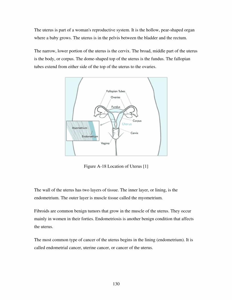
130
The uterus is part of a woman's reproductive system. It is the hollow, pear-shaped organ
where a baby grows. The uterus is in the pelvis between the bladder and the rectum.
The narrow, lower portion of the uterus is the cervix. The broad, middle part of the uterus
is the body, or corpus. The dome-shaped top of the uterus is the fundus. The fallopian
tubes extend from either side of the top of the uterus to the ovaries.
Figure A-18 Location of Uterus [1]
The wall of the uterus has two layers of tissue. The inner layer, or lining, is the
endometrium. The outer layer is muscle tissue called the myometrium.
Fibroids are common benign tumors that grow in the muscle of the uterus. They occur
mainly in women in their forties. Endometriosis is another benign condition that affects
the uterus.
The most common type of cancer of the uterus begins in the lining (endometrium). It is
called endometrial cancer, uterine cancer, or cancer of the uterus.
131
REFERENCES
1. www.cancer.gov
2. http://www.geocities.com/HotSprings/Villa/5443/alts/hytherm.html
3. O. S. NIELSEN, M. HORSMAN, J. OVERGAARD, European J. of Cancer, 37
(2001) 1587-1589
4. http://cis.nci.nih.gov/fact/7_3.htm
5. B. HILDEBRANDT, PETER WUST Crit. Reviews in Oncology/Hematology, 43
(2002) 33-56
6. B. PARK, B. S. KOO, Y. K. KIM, M. K. KIM, Korean J Radiol, 3 (2002) 98-104
7. S. DEGER, D. BOEHMER, I. TURK, J. ROIGAS, V. BUDACH, S. LOENING,
European Urology, 42 (2002) 147-153
8. A. JORDAN, R. SCHOLZ, P. WUST, H. FAHLING. R. FELIX, J Mag Mag
Matr, 201 (1999) 413-419
9. N. BRUSENTSOV, L. NIKITIN, T. BRUSENTSOVA, A. KUZNETSOV, F.
BAYBURTSKIY, L. SCHUMAKOV, N. JURCHENKO, J. Mag. Mag. Matr.,
252 (2002) 378-380
10. C. C. BERRY, ADAM S. G. CURTIS, J. Phys. D: Appl. Phys. 36 (2003) R198-
R206
11. YOED RABIN, Nanotechnology Essays, (2003)
12. R. HERGT, W. ANDRA, C. G. D’AMBLY, I. HILGER, W. A. KAISER, U.
RITCHER, HANS-GEORG SCHMIDT, IEEE Trans. On mag., 34-5, (1998)
3745-3754
13. BRUCE M. MOSKOWITZ, Hitchhiker’s Guide to Magnetism
14. http://yarchive.net/metal/magnetic_materials.html

132
15. H. S. NALWA, Handbook of Nanostructured Materials and Nanotechnology Vol
1, 3-4
16. E. AUZANS, Thesis: Mn-Zn Ferrite nanoparticles for water and hydrocarbon
based ferrofluids: preparation and properties, Institute of Physics of Latvian
University
17. http://www.elidis.cz/en/vzacne.htm
18. R. V. UPADHYAY, R. V. MEHTA, K. PAREKH, D. SRINIVAS, R. P. PANT,
J. of Mag. Mag. Matr., 201, (1999) 129-132
19. P. KINNARI, R. V. UPADHYAY, R. V. MEHTA, J. of Mag. Mag. Matr., 252
(2002) 35-38
20. H. S. NALWA, Handbook of Nanostructured Materials and Nanotechnology Vol
1, 17
21. L. K. KURIHARA, G. M. CHOW, P. E. SCHOEN, Nanostructured Mat. Vol 5, 6
(1995) 607-613
22. G. M. CHOW, L. K. KURIHARA, Chem synth and processing of nano powders
and films
23. M. B. LILLY, I. A. BREZOVICH, W. J. ATKINSON, Radiology 154, (1985)
243-244.
24. Scintag: Basics of X-Ray Diffraction, http://epswww.unm.edu/xrd/xrdbasics.pdf
25. A. NIAZI, P. PODDAR, A. K. RASTOGI, A Precision low-cost vibrating sample
magnetometer.
26. http://whatis.techtarget.com/definition/0,,sid9_gci816722,00.html
27. http://www.abdn.ac.uk/physics/case/squids.html
28. http://www.unl.edu/CMRAcfem/temoptic.htm
29. D. FIORANI, H. ROMERO, L. SUBER, A. M. TESTA, M. VITTORI, A.
MONTONE, J. L. DORMANN, J. MAKNANI, Matr. Sci. and Engg., A204,
(1995) 165-168
30. G. D. FORSTER, Q. A. PANKHURST, I. P. PARKIN, J. of Matr. Sci. Letters,
18, (1999) 39-40
31. P. FULMER, J. KIM, A. MANTHIRAM, J. M. SANCHEZ, ANRCP, 15, (1999)

133
32. J. SMIT AND H. P. J. WIJN, Ferrites, John Wiley & Sons, NY, 1959, 139-142
33. C. KITTEL, Intro. To Solid State Physics, John Wiley & Sons, NY, 4th
Ed.
34. G. BURNS, Solid State Physics, Academic Press Inc.,1985
35. K. SCHRODER, Elec., Mag. And Thermal Properties of Solid Mat., Marcel
Dekker Inc. NY, 1978
36. R. KUBO, T. NAGAMIYA, Solid State Physics, McGraw Hill., 1969
37. J. SMIT AND H. P. J. WIJN, Ferrites, John Wiley & Sons, NY, 1959, 139-142
38. K. A. GSCHNEIDNER JR., A. PECHARSKY, K. W. DENNIS, J. of Alloy and
Comp., 260, (1997) 107-110
39. R. GREF, A. DOMB, P. QUELLEC, T. BLUNK, R. H. MULLER, J. M.
VERBAVATZ, R. LANGER, Advanced Drug Delivery reviews, 16 (1995) 215 –
233
40. A. K. GUPTA, S. WELLS, IEEE Trans. On Nanobioscience, 3 (2004) 66 – 73
41. M. CHASTELLAIN, A. PETRI, H. HOFMANN, J. of Colloid and Interface
Science, 278 (2004) 353 – 360
42. A. VILLA, H. GILL, O. MCCALLION, M. J. ALONSO, J. of Controlled
Release, 98 (2004) 231 – 244
43. G. RUAN, S. FENG, Biomaterials, 24 (2003) 5037 – 5044
44. G. RUAN, S. FENG, Q. LI, J. of Controlled Release, 84 (2002) 151 – 160
45. J. CHATTERJEE, Y. HAIK, C. J. CHEN, J. Mag. Mag. Matr., 225 (2001) 21 –
29
46. R. SOLARO, Nanostructured Polymeric Systems in Targeted Release of Proteic
Drugs and in Tissue Engineering
47. J. W. VANDERHOFF, M. S. ASSER, J. UGELSTAD, US Patent: 4,177,177
48. A. M. NEJAD, A. A. M. MOVAHEDI, S. SAFARIAN, Thermochimica Acta, 389
(2002) 141-151

134
BIOGRAPHICAL SKETCH
Virendra Mohite
Department of Mechanical Engineering
FAMU-FSU College of Engineering
2525 Pottsdamer Street, Tallahassee, FL – 32310
Education
MS Mechanical Engineering (Aug 2002 – Dec 2004)
Florida State University, Tallahassee, FL
Bachelor of Engineering, Mechanical Engineering (Aug 1997 – Jul 2001)
Mumbai University, Mumbai, India
Professional Experience
Research Assistant (Jan 2002 – Dec 2004)
Center for Nanomagnetics and Biotechnology
Mechanical Engineer (May 2001 – Jul 2002)
Rigimax m/c tools pvt. ltd.
Mumbai, India
Mechanical Engineering Intern (May 2000 – May 2001)
Rigimax m/c tools pvt. ltd.
Mumbai, India

135
Personal Information
Date of Birth: 17th
Jan 1980
Place of Birth: Mumbai, India
Contact Information
E-Mail: [email protected], [email protected]