self-consistent description of nuclear excitations - progress of

330 Supplement of the Progress of Theoretical Physics, Nos. 74 & 75, 1983

Self-Consistent Description of Nuclear Excitations

Nguyen Van GIAI

Division de Physique Theorique*> Institut de Physique Nucleaire, 91406 Orsay Cedex

(Received July 11, 1982)

The nuclear response function is calculated in the framework of the selfconsistent continuum RPA. The method is illustrated by applications to lowlying collective states, and to various isoscalar giant resonances.

§ l. Introduction

The study of nuclear excitations in the energy region of a few ha>-the so-called giant resonance region-has been, and still is one of the most active fields of nuclear physics. In the last ten years, the large amount of experimental effort has led to a fairly good systematics of electric (non-spin-flip) giant resonances.D This effort is still going on, and it will eventually bring a more complete knowledge of electric giant resonances along with our developing understanding of magnetic (spin-flip) resonances. At the same time, various theoretical approaches ranging from fluid dynamics to microscopic models have aimed at describing the observed resonances. In this paper we shall focus on one particular approach, namely, the self-consistent RPA modeL

An interesting feature of the RPA is its well-known ability to let the collective character of the excitations emerge from the properties of the residual interactions, in contrast to non-microscopic models where the collectiveness is built-in from the start. On the other hand, the RPA model has its own limitations. For instance, we know that the actual states contain admixtures of complex configurations outside the RPA space and they are consequently more fragmented than the RPA would predict. This question is discussed in Yoshida's lectures!> Nevertheless, the RPA has proved to be quite successful in describing the bulk properties of giant resonances such as their energies and strengths.

There are traditionally two ways of considering the RP A modeL In the first one, the two main inputs are treated separately, i.e., the single particle energies are taken "from experiment" whereas the residual interaction is phenomenologically adjusted and sometimes supplemented by meson-exchange forces. In the second one-the self-consistent RPA-the emphasis is put on the fact

*> Laboratoire associe au C.N.R.S.

Dow

nloaded from https://academ

ic.oup.com/ptps/article/doi/10.1143/PTPS.74.330/1912904 by guest on 23 January 2022

Self-Consistent Description of Nuclear Excitations 331

that both the single particle quantities and the residual interaction must be

derived from the same effective two-body force. This requirement seems quite natural if one sees the RPA as the small amplitude limit of the Time Dependent Hartree-Fock approximation. Also, it allows a close comparison between detailed RPA results and more global predictions of sum rule methods8>

based on the self-consistency assumption. In the following, we shall discuss some predictions of the self-consistent

RPA using Skyrme type interactions. For the sake of completeness, we recall the method of calculation first proposed by Bertsch and Tsai.4> We then illustrate it by calculating the low lying collective states in 208Pb and comparing them with experimental data. Next, we examine the results for various giant resonances calculated in the continuum RPA method. In this paper, we concentrate on the case of non-spin-flip isoscalar states and giant resonances. Applications of the self-consistent RPA to isovector dipole resonances and to

spin-flip resonances (Gamow-Teller, M1) are discussed in the talks of Bohigas5>

and Sagawa.8>

§ 2. General method

The method of Ref. 4) takes advantage of the fact that for interactions

of the Skyrme type, the RPA equations can be numerically solved in coordinate space. This is interesting because one thus avoid expansions on discrete basis and their related space 'truncation problems. Furthermore, the single particle continuum can be handled exactly and our RPA states contain there

fore the effects of particle escape.

2. 1. The particle-hole Green's function Let us assume that the Hartree-Fock (HF) problem has been solved for

some effective interaction Y12• We then know the HF hamiltonian H 0, its

eigen-energies ei and Sm (subscripts i, j, · · · and m, n, · · · stand for occupied and unoccupied states, respectively) and the corresponding wave functions ({Ji and

9m· Above some threshold, m becomes a continuous index. In the familiar configuration representation, the non-interacting particle

hole Green's function G<D> has the form,

where E is the excitation energy. We now transform c<o> to the coordinate

representation and look at the speci~;tl case where the particle-hole pair sits at the same point in space:

c<o) Crt, r2, E)

= :E 9i* Crt) 9m Crt) [ 1 E . mi em-ei- -t"fj

Dow



332 Nguyen Van Giai

For each hole state i, we must calculate quantities of the form l:m (/Jm (r1)

Xq;m*(r2)/(sm-St±E-ir;), which are just the one-body Green's functions 1/ (H0 -St ± E- ir;) in r-representation, except for the hole-hole terms 2:;1

q;1 (r1) q;/ (r2) / (s1 - St ± E- ir;) which can be readily subtracted (in fact, this is taken care of by the two terms in Eq. (2) because their hole-hole contributions cancel out mutually).

The next thing to notice is that for Skyrme forces the HF Hamiltonian H 0 is a purely differential operator, the non-locality of the HF field being

contained in an effective mass m* (r). We can then express the Green's function of such a differential operator in a closed form :7)

(3)

where r< and r> stand respectively for r1 and r 2 if r 1<r2, and for r 2 and r1 if r 2<r1 • In Eq. (3), z is a real parameter, u and v are two linearly inde

pendent solutions of (H0 -z)u=0, W(u, v) is the Wronskian of these solutions. At the origin, u and v are respectively regular and irregular, whereas at infinity we require v to be a spherically outgoing wave. By using Eqs. (2) and (3) we can thus obtain the Green's function G(Ol in the untruncated parti

cle-hole space and we have not discretized the continuous spectrum.

2. 2. The RP A Green's function If we denote by Vph the residual particle-hole interaction that one can con

struct from the interaction V12 by functional differentiation of the HF Hamiltonian,<) we can write the integral equation for the RPA Green'~ function as

GRPA (E) = G(O) (E) - c<o) (E) vphGRPA (E). (4)

For Skyrme type forces, this can be reduced to a single one-dimensional integral equation in r-space for each multipolarity L~, and one can solve it

numerically to obtain ~PA (l't. r 2 ; E). The spectral representation of GRPA is similar to that of G(Ol (see Eq.

(2)), i.e.,

GRPA(rt, r2;E) =:I; <1>ol¢t(ri)¢(ri) I¢N)<¢NI¢t(r2)¢(r2) lr/>o) N

(5)

where ¢0 is the RPA ground state, (/JN and EN the excited eigenstates and eigenenergies, cpt (r) (cjJ (r)) is the field operator which creates· (annihilates) a

nucleon at point r. The subscript N becomes a continuous index when En is above the particle emission threshold. One recognizes in the numerator of Eq. (5) the product of transition demities PNo at points r 1 and r 2•

Dow




2. 3. Strength distributions From Eq. (5) we see that the analytic structure of GRPA consists of

discrete poles on the real E-axis at the energies of the RPA bound states,

and a cut starting from the particle emission threshold. For a given value

of the excitation energy E, the corresponding local transition density PNo (r1)

can be obtained by appropriately integrating GRPA (r1, r 2 ; E) over r 2•

In general, one is interested in calculating the strength distributions

S(E) ='L:NI<¢o[Q[¢N)[ 26(E-EN) corresponding to one-body local operators

Q(r) =f(r) YLM(r) (the notation 'L:N includes integration over the continuous

parameter EN above threshold) . This can be done by looking at the response

function:

(6)

For a discrete state the transition strength is the residue of RQ (E) at the pole

E =EN, whereas above threshold S (E) is 1/n times the imaginary part of

RQ (E) . The response function RQ, or the strength distribution S, may become

particularly large whenever the energy E, which can be considered as a

"tuning parameter", hits a collective state or a giant resonance. Examples

of such calculations of S(E) which include both self-consistency and continuum

effects can be found, e.g., in Ref. 8).

§ 3. Low-lying collective states

We begin with an application of the above formalism to the low-lying spec

trum of 208Pb. The calculations are performed with the Skyrme force Sill

which was originally adjusted to ground state properties in the HF approximation.9>

In the low energy region (E<hw) several RPA states appear to be

strongly collective. Their electromagnetic transition strengths are several tens

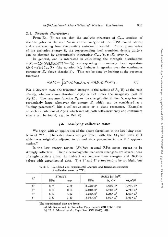
of single particle units. In Table I we compare their energies and B(EL) values with experimental data. The 2+ and 4+ states tend to be too high, but

L"

Table I. Calculated and experimental energies and transitions strengths of collective states in ""Pb.

E[MeV] B(EL) [e'·fm'L]

RPA exp. RPA (e, e')a> (a, a')bl

6.05 4.07 3. 44X 10' 2. 96 X10' 3. 70Xl0'

3.00 2.63 5. 60X10' 7.72xl0' 7.74X10'

6.60 4.32 1. 03 X10' 1. 29 X10' 1. 60X 107

3.80 3.19 3. 36X 108 4. 51 Xl08 5.64Xl08

The experimental data are from : a) M. Nagao and Y. Torizuka, Phys. Letters 37B (1971), 383. b) H. P. Morsch et al., Phys. Rev. C22 (1980), 489.

Dow



334

4+ 4.32MeV

•. + .. II I ...

0.1

6' 10 10

Nguyen Van Giai

T 2.63MeV

--Mod1 ·····Mod 2

-·-·-Mod 3

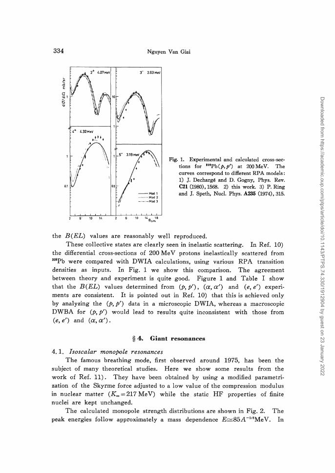
Fig. 1. Experimental and calculated cross-sections for 108Pb (p, p') at 200 MeV. The curves correspond to different RP A models : 1) ]. Decharge and D. Gogny, Phys. Rev. C21 (1980), 1568. 2) this work. 3) P. Ring and ]. Speth, Nucl. Phys. A235 (1974), 315.

the B(EL) values are reasonably well reproduced. These collective states are clearly seen in inelastic scattering. In Ref. 10)

the differential cross-sections of 200 MeV protons inelastically scattered from 208Pb were compared with DWIA calculations, using various RP A transition densities as inputs. In Fig. 1 we show this comparison. The agreement between theory and experiment is quite good. Figure 1 and Table I show that the B(EL) values determined from (P, p'), (a, a') and (e, e') experiments are consistent. It is pointed out in Ref. 10) that this is achieved only by analyzing the (P, p') data in a microscopic DWIA, whereas a macroscopic DWBA for (p, p') would lead to results quite inconsistent with those from (e, e') and (a, a').

§ 4. Giant resonances

4. 1. Isoscalar monopole resonances The famous breathing mode, first observed around 1975, has been the

subject of many theoretical studies. Here we show some results from the work of Ref. 11). They have been obtained by using a modified parametrization of the Skyrme force adjusted to a low value of the compression modulus in nuclear matter (Koo = 217 MeV) while the static HF properties of finite nuclei are kept unchanged.

The calculated monopole strength distributions are shown in Fig. 2. The peak energies follow approximately a mass dependence E=85A - 118Me V. In

Dow




Table II. Energies and widths (in MeV) of monopole resonances. Besides the peak energies are also shown the centroid energies E, full width at half maximum r and variance q_

Nucleus

Epeak

E r q

30 SCEJ [fm' MeV''] "Ca

20

10

150 "'Zr

m

50

1.5.10' "'Pb

35

... Ph

14.6 15.3 1.7 2.1

••zr ••ca

18.5 --23. 19.5 22.7 2.6 >7. 3.0 5.0

Table II are summarized the mam features

of the strength distributions.

When going from heavy to lighter

nuclei, the widths of the distributions, i.e.,

the particle escape widths, increase rapidly.

In 208Pb, the calculated escape width is more

than half of the observed total width (Fexp

=3.0 MeV). This is consistent with the

fact that the spreading width is strongly

quenched for isoscalar monopole states.m,tsJ

In 4°Ca, the distribution is very broad.

Experimentally, only bits and pieces of

monopole strength have been measured in

A:s;58 nuclei but nothing like a strong

resonance. Figure 2 shows that the con

tinuum RPA does not indeed predict any

concentration of strength in 4°Ca. The

effects of 2 particle-2 hole configurations

are not likely to change this situation.

The shapes of RP A transition densities

PNo (r) are similar to that of the Tassie

model, 3p + rdpj dr. However, the RPA

values of PNo (r) tend to be larger than that

Fig. 2. Monopole strength distributions calculated with interaction SGII.

of the Tassie model in the outer surface

region. It would be interesting to see whether this feature could bring the

calculated cross sections for (a, a') (which are too small when the Tassie

model is used141 ) to a better agreement with experiment.

4. 2. Isoscalar dipole resonances

The dipole compression modes have also been calculated in Ref. 11)

using the same interaction as in the monopole case. For these L~=l-, LIT=O excitations, it is quite important to fulfil the self-consistency requirement.

Indeed, the center-of-mass state would then separate out from the physical

Dow



336 Nguyen Van Giai

states and become degenerate with the ground state, by virtue of Thouless theorem.

In Fig. 3 are shown the strength distributions for the dipole operator ~Y10 (r). The resonance energies and widths are listed in Table III. Apart from small concentrations of strength around 15 MeV, one sees a main peak which is broader than the monopole resonance. It becomes very broad in the Ca region. The peak energies have the approximate-A-dependence E=150 A-118MeV.

Table III. Energies and widths (in MeV) of isoscalar dipole resonances .

SCEl

1!10

100

50

1.5.~

0.5o1o'

Nucleus

Epeak

E r

30E[MeV]~

40Ca

"'Pb

••• Pb

25.9 22.5 3.2 5.4

Fig. 3. Dipole strength distributions calculated with interaction SGII.

~

••zr

""33.

28.1 6.8 7.9

{------' ' ' ' ' ' ' '

••ca

29~38

27.6

""20. 11.2

0~n~----~----~----~ .. ----~~,-'•"-f-~l 10',.-r---------,-------,---------,

1: ol I' ,\ /

M' '' ,v 11· V' \ 11 / j· ' .. _ ... , __ ~ .........

Fig. 4. B(EL) values in ••ca. The units are in fmiL MeV-'. In the upper part of the figure are the integrated energy-weighted strengths for L=2 (dashed curve), L=3 (solid curve) and L=4 (dot-and-dashed curve).

Dow




For the present dipole operator, the energy-weighted sum rule (EWSR) corrected for center of mass effects is:

(7)

In 208Pb and 90Zr, the giant resonance exhausts respectively 58% and 73% of m1- In 4°Ca, the broad structure extending over a 20 MeV range contains about 70% of m 1• Experimentally, the analysis10> of 200 MeV proton scattering from 208Pb indicates that an isoscalar dipole resonance is located around 21.5 MeV. It has a total width of 5.7 MeV and it exhausts about 70% of

The radial shape of the transition density calculated in RPA has a node in the surface region. This shows that the isoscalar dipole resonance is a mode in which matter is compressed and expanded along some direction. The RPA transition density is similar to that derived from the sum rule approach :15>

(8)

but they differ in details. Because of the node in PNo (r), one can expect that the strength distribution of operators like j 1 (qr) Y10 (r) will have a strong qdependence. This property might be useful for distinguishing the isoscalar dipole from other resonances in the same energy region.

4. 3. L = 2, 3 and 4 resonances Response function calculations which are self-consistent but without con

tinuum effects have been reported in details in Ref. 16) for multipoles up to L = 4. Here, we discuss some results which include the continuum effects, in the case of 4°Ca. To make the calculations simpler, however, we have not used the full Vph derived from the Skyrme force but we have kept only the Fo and Go parts in the Landau-Migdal expansion of Vph· The neglect of F1 and G1 leads to a residual interaction which is more attractive, but this approximation is nevertheless sufficient for our qualitative discussion. The parameters of the force Sill have been used for the calculations.

In Fig. 4 are shown the B(EL) values (i.e., the distributions S(E) for multipole operators rLYLo (r)) as functions of the excitation energy E. The integrated energy-weighted strengths are also shown in the upper part of the figure. For L = 2, a narrow resonance exhausting a very large fraction of EWSR lies at 15 MeV. In a fully self-consistent calculation with the same interaction Sill, we find this resonance at 17 MeV, which can be understood

by the difference between Vph and its approximation by Fo + G0u1 • u2. We can therefore conclude that the force Sill can satisfactorily reproduce the quadrupole energy, but the continuum width is negligibly small as compared tGJ the observed width.

Dow



338 Nguyen Van Giai

For L = 3, some small structures exist around 18 MeV but the mam part

of the strength is in a bump of 4 MeV wide with its peak at E=30 MeV.

More complex configurations will fragment out this bump, so that the main

octupole strength might be in a wide energy range between 2 h(J) and 3 h(J). The L = 4 strength exhibits several structures in the 20 to 40 MeV region,

the strongest one being at 22 MeV, but altogether they exhaust only half of

the EWSR. From 40 to 45 MeV, the L=4 curve in the upper part of Fig.

4 increases rapidly, i.e., a large fraction of strength (25% of EWSR) is pre

dicted in that region. Again, damping effects would spread out further the

RPA strength and therefore the L = 4 states would appear as many small

resonances over a wide range of energy.

When one looks at this kind of theoretical predictions, one must however

remember that they do not necessarily correspond to the excitation functions

observed in inelastic electron or hadron scattering. This is because the

B(EL)-values are related only to the zero momentum limit of transition form

factors, whereas the actual excitation functions certainly involve finite values

of momentum transfer q. A calculation of d 2rJ j dQdE would be the appropriate

thing to do, but this is quite beyond the scope of the present study. We can,

however, look at the behaviour of the form factors at finite momentum transfer

by calculating the response to the operator jL (qr) YLo (r). The corresponding

strength distributions are shown in Fig. 5 (L = 2 and L = 3) and Fig. 6

(L=4). For a finite but small value of momentum (q = 0.5 fm- 1), the distributions

are similar to the B(EL) distributions in all three cases. For q = 1.5 fm- 1

the distributions are strongly changed in the L = 2 and L = 3 cases and to a

lesser extent in the L = 4 case. For L = 2, the resonance at 15 MeV is no

longer prominent whereas several structures in the 20'"'""30 MeV region become

10° ..--.--,.--r--.-....

m""

10_,

L.2 ----- q ,Q,S fm-1 _ q,1.5fm~

10-'

m·•

10 20 30 40 so 60 E (MeV)

Fig. 5. Strength distributions of the operator jL(qr)YLo(r), for L=2 (left) and L=3 (right).

Dow



1o-3

10-4

1o-5

I I • • II

" " 10-6 " 10


20 30 40

L = 4

q =0.5 fm-1 q = 1.5 fm-1

50 60 E{MeV)

Fig. 6. Strength distribution of the operator j. (qr) Y., (f).

important. For L = 3, the resonance at 43 MeV becomes comparable in strength with the one at 30 MeV. For L = 4, the change is not so big, but there is a resonance at 30 MeV which increases quickly in that range of q. In all three cases there are no significant structures above 45 MeV, but for larger q

the strength decreases more slowly as E increases. From these results we can conclude that the RPA model does not predict strongly collective resonances above the 3h(J)"-'4h(J) region for L< 4 isoscalar modes.

4. 4. Resonances of higher multipolarities One might wonder whether the energies of giant resonances will keep

increasing as the multipolarity L increases. The particle-hole model based on the harmonic oscillator tells us that the strength distribution of the multipole operator rLYL is peaked around Lh(J) (L>2). However, the harmonic oscillator can be quite misleading for large L. In fact, one can easily evaluate the centroid energies for various L in a finite well or a HF potential.m The result is that these centroid energies are much lower than predicted by the harmonic oscillator when L is large, and they do not depend much on L.

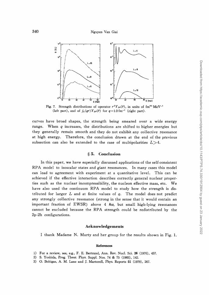
We have performed RPA calculations of L = 6, 8 and 10 states in 4°Ca, using the same approximation for "Vph as in the previous subsection. Indeed, for such large multipolarities the residual interaction is unimportant, and the strength distributions of RPA and particle-hole models are quite similar. In Fig. 7 we show the B(EL) values (left part) and the strength distributions of the operators jL (qr) YL (r) for the choice of q = 1.0 fm _, (right part). The L = 6 case shows some structure, especially for the finite value of q, but the other cases are quite structureless. The left part of Fig. 7 illustrates what we said above, i.e., the centroid (and peak) energies are quite low. The

Dow



340

1016

::r !!!.

101!'>

101'

1013

Nguyen Van Giai

2030/IJ5060 E (MeV)

Fig. 7. Strength distributions of operator rLYLo(r), in units of fm'L MeV-' Cleft part), and of jL(qr)YLo(r) for q=l.Ofm-' (right part).

curves have broad shapes, the strength being smeared over a wide energy range. When q increases, the distributions are shifted to higher energies but they generally remain smooth and they do not exhibit any collective resonance at high energy. Therefore, the conclusion drawn at the end of the previous subsection can also be extended to the case of multipolarities L>4.

§ 5. Conclusion

In this paper, we have especially discussed applications of the self-consistent RPA model to isoscalar states and giant resonances. In many cases this model can lead to agreement with experiment at a quantitative level. This can be achieved if the effective interaction describes correctly general nuclear properties such as the nuclear incompressibility, the nucleon effective mass, etc. We have also used the continuum RPA model to study how the strength is distributed for larger L and at finite values of q. The model does not predict any strongly collective resonance (strong in the sense that it would contain an important fraction of EWSR) above 4 Ita>, but small high-lying resonances cannot be excluded because the RPA strength could be redistributed by the 2p-2h configurations.

Acknowledgements

I thank Madame N. Marty and her group for the results shown in Fig. 1.

References

1) For a review, see, e;g., F. E. Bertrand, Ann. Rev. Nucl. Sci. 26 (1976), 457. 2) S. Yoshida, Prog. Theor. Phys. Suppl. Nos. 74 & 75 (1983), 142. 3) 0. Bohigas, A. M. Lane and ]. Martorell, Phys. Reports 51 (1979), 267.

Dow




4) G. F. Bertsch and S. F. Tsai, Phys. Reports 18C (1975), 125. S. F. Tsai, Phys. Rev. C17 (1978), 1862.

5) 0. Bohigas, Prog. Theor. Phys. Suppl. Nos. 74 & 75 (1983), 380. 6) H. Sagawa, Prog. Theor. Phys. Suppl. Nos. 74 & 75 (1983), 342. 7) R. Courant and D. Hilbert, Methods of Mathematical Physics (Interscience Publishers,

New York, 1953). 8) K. F. Liu and Nguyen Van Giai, Phys. Letters 65B (1976), 23. 9) M. Beiner et al., Nucl. Phys. A238 (1975), 29.

10) C. Djalali, N. Marty, M. Morlet and A. Willis, Nucl. Phys. A380 (1982), 42. 11) Nguyen Van Giai and H. Sagawa, Nucl. Phys. A371 (1981), 1. 12) G. F. Bertsch, Phys. Letters 37B (1971), 470.

H. Ui, Proceedings of the Kawatabi Conference on New Giant Resonances, Sendai, 1975, p. 105.

13) P. F. Bortignon and R. A. Broglia, Nucl. Phys. A371 (1981), 405. 14) F. E. Bertrand et a!., Phys. Rev. C22 (1980), 1832, 15) M. N. Harakeh and A. E. L. Dieperink, Phys. Rev. C23 (1981), 2329. 16) K. F. Liu and G. E. Brown, Nucl. Phys. A265 (1976), 385. 17) Nguyen Van Giai, Phys. Letters 105B (1981), 11.

Dow



self-consistent description of nuclear excitations - progress of

Documents