self-aggregation of convection in long channel...
TRANSCRIPT
Self-Aggregation in Channel Geometry 1
Self-aggregation of convection in long channel geometry
Allison A. Wing a∗, Timothy W. Cronin b
aLamont-Doherty Earth Observatory, Columbia University, PO Box 1000, Palisades, NY 10960
bDepartment of Earth and Planetary Science, Harvard University, 20 Oxford St., Cambridge, MA 02138.
∗Correspondence to: Allison A. Wing, Lamont-Doherty Earth Observatory, Columbia University, PO Box 1000, Palisades, NY
10960, USA.
Cloud cover and relative humidity in the tropics are strongly influenced by organized
atmospheric convection, which occurs across a range of spatial and temporal scales.
One mode of organization that is found in idealized numerical modeling simulations
is self-aggregation, a spontaneous transition from randomly distributed convection
to organized convection despite homogeneous boundary conditions. We explore the
influence of domain geometry on the mechanisms, growth rates, and length scales of
self-aggregation of tropical convection. We simulate radiative-convective equilibrium
with the System for Atmospheric Modeling (SAM), in a non-rotating, highly-elongated
3D channel domain of length > 104 km, with interactive radiation and surface fluxes
and fixed sea-surface temperature varying from 280 K to 310 K. Convection self-
aggregates into multiple moist and dry bands across this full range of temperatures.
As convection aggregates, we find a decrease in upper-tropospheric cloud fraction, but
an increase in lower-tropospheric cloud fraction; this sensitivity of clouds to aggregation
agrees with observations in the upper troposphere, but not in the lower troposphere. An
advantage of the channel geometry is that a separation distance between convectively
active regions can be defined; we present a theory for this distance based on boundary
layer remoistening. We find that surface fluxes and radiative heating act as positive
feedbacks, favoring self-aggregation, but advection of moist static energy acts as a
negative feedback, opposing self-aggregation, for nearly all temperatures and times.
Early in the process of self-aggregation, surface fluxes are a positive feedback at
all temperatures, shortwave radiation is a strong positive feedback at low surface
temperatures but weakens at higher temperatures, and longwave radiation is a negative
feedback at low temperatures but becomes a positive feedback for temperatures greater
than 295-300 K. Clouds contribute strongly to the radiative feedbacks, especially at low
temperatures.
Key Words: Convection, Self-Aggregation, Radiative-Convective Equilibrium, Tropical Clouds
Received . . .
c© 2015 Royal Meteorological Society Prepared using qjrms4.cls

Quarterly Journal of the Royal Meteorological Society Q. J. R. Meteorol. Soc. 00: 2–?? (2015)
1. Introduction
Tropical clouds and relative humidity play a key role in both
the planetary energy balance and the sensitivity of global climate
to radiative forcing. A large fraction of tropical cloudiness and
rainfall (approximately 50% (Nesbitt et al. 2000; Tan et al.
2013)) is associated with organized convection, and recent
work suggests that the frequency of organized convection in
the tropics is increasing with warming (Tan et al. 2015). It
has been recently suggested that some modes of convective
organization may result from an instability of the background state
of radiative-convective equilibrium, which results in separation of
the atmosphere into moist regions with ascent and dry regions with
subsidence (Emanuel et al. 2014). If such an instability indeed
exists in the real atmosphere, it would reshape our understanding
of tropical circulations, and could help to explain the growth
and life cycle of large-scale organized convective systems such
as tropical cyclones and the Madden-Julian Oscillation (e.g.,
Bretherton et al. 2005; Sobel and Maloney 2012). If this instability
is temperature-dependent, as suggested by numerical modeling
studies (Khairoutdinov and Emanuel 2010; Wing and Emanuel
2014; Emanuel et al. 2014), then the increasing tendency of
convection to organize with warming could also alter the climate
sensitivity significantly (Khairoutdinov and Emanuel 2010); it
is unclear whether current global climate models capture this
process adequately.
In this paper, we use self-aggregation to mean the spontaneous
transition in a model from a state of homogenous convection
and rainfall, to a state of heterogeneous convection and rainfall,
with homogeneous boundary conditions. With this definition,
self-aggregation is widespread in numerical models of the
atmosphere that are forced with spatially homogeneous sea-
surface temperatures and insolation. Self-aggregation occurs in
models with high resolution and varied geometry, from 2D (Held
et al. 1993; Grabowski and Moncrieff 2001, 2002; Stephens et al.
2008), to small-domain square 3D (Tompkins and Craig 1998;
Bretherton et al. 2005; Muller and Held 2012; Jeevanjee and
Romps 2013; Wing and Emanuel 2014), to elongated channel
3D (Posselt et al. 2008; Stephens et al. 2008; Posselt et al.
2012), as well as regional or global models with parameterized
clouds and convection (Su et al. 2000; Held et al. 2007; Popke
et al. 2013; Becker and Stevens 2014; Reed et al. 2015). The
spontaneous symmetry-breaking suggested by the 2-dimensional
latitude-height study of Raymond (2000) and by the 2-column
model of Nilsson and Emanuel (1999), as well as the existence
of multiple equilibria in single-column (Sobel et al. 2007)
and 2D cloud resolving (Sessions et al. 2010) simulations
employing the weak temperature gradient approximation, may
also be interpreted as falling under this broad definition of self-
aggregation of convection. There is also observational evidence
for the dependence of the area-average atmospheric state on
the degree of aggregation of convection that is in some ways
consistent with numerical simulations (Tobin et al. 2012, 2013).
Is the phenomenon of self-aggregation in a 200 km × 200 km
domain in a model with explicit convection and clouds possibly
the same as that in a 20000 km × 20000 km domain in a model
with parameterized convection and clouds? This question has
largely gone unaddressed, but it is essential to answer if we want to
understand the robustness of self-aggregation across our modeling
hierarchy and its relevance to the real atmosphere. We seek to
address this question by focusing on the following three goals:
1. To investigate the details of self-aggregation across
temperatures in long channel geometry by quantifying its
growth rates, physical mechanisms, and length scales
2. To compare these findings to previous results in square
geometry and available observations
3. To propose a theory for the length scale of self-aggregation
based on the temperature dependence of the size of multiple
moist and dry bands that develop in channel geometry.
Non-rotating simulations of square domains with side lengths
less than 1000 km form the bulk of the body of previous work
on self-aggregation, but they have given at most one convectively
active region within the domain, and have thus failed to identify
any length scales of self-aggregation that differ from the limits
imposed by the domain. This is disconcerting because the growth
rates and length scales of dynamical instabilities are generally
interrelated, so the suppression of wavelengths larger than the
domain size may also artificially truncate unstable modes that
could exist in the real tropical atmosphere. To avoid these
c© 2015 Royal Meteorological Society Prepared using qjrms4.cls
Self-Aggregation in Channel Geometry 3
problems, we use a long channel setup similar to Posselt et al.
(2008), which allows aggregation to occur across a much broader
range of length scales than in square geometry.
Previous studies of self-aggregation are briefly reviewed in
Section 2. Section 3 describes our model setup, and Section 4
presents basic results. We describe our analysis framework and
apply it to the model results in section 5. Section 6 introduces
a simple model for a remoistening length scale relevant for
aggregation, and section 7 places our results in the context of
previous studies, emphasizing comparison to square geometry.
The paper concludes with a summary in Section 8.
2. Literature Review
In cloud-resolving simulations of radiative-convective equilibrium
(RCE) over square 3D domains, with side lengths being hundreds
of kilometers, self-aggregation has usually manifested as a single
intensely precipitating cluster, surrounded by dry, subsiding air.
Bretherton et al. (2005) and Muller and Held (2012) argued that
convection–moisture–radiation feedbacks, which dry the drier air
columns and moisten the moister air columns, are critical for
self-aggregation; Wing and Emanuel (2014) clarified that clear-
sky longwave radiation and wind-driven surface flux feedbacks
dominate the early stages of aggregation. But our understanding
of self-aggregation based on these results from square 3D domains
has been complicated by the sensitivity of the existence of
aggregation to domain size, horizontal resolution, and temperature
(Muller and Held 2012; Jeevanjee and Romps 2013; Wing and
Emanuel 2014). As reviewed below, self-aggregation may be more
robust when model configurations are employed that include at
least one side length O(104) km.
In the small (640 km) cloud-resolving 2D simulations of Held
et al. (1993), convection aggregated only when x-averaged winds
were constrained to vanish, and could be destroyed by a small
amount of vertical wind shear. Grabowski and Moncrieff (2001)
also found self-aggregation in a much larger (20,000 km) 2D
domain, at multiple scales and into multiple clusters. Large-
scale aggregation occurred despite fixed radiative cooling and
was attributed to convective momentum transport and its effects
on surface processes. Grabowski and Moncrieff (2002) found
that interactive radiation increased the strength of aggregation,
as quantified by the spatial variance of precipitable water, and
caused the larger envelope of convection to follow the mean flow;
aggregation was not destroyed by vertical wind shear, but its
characteristics were altered.
A small number of studies have simulated self-aggregation
in elongated 3D channel geometry with cloud-resolving models,
which allows for both large scale overturning circulations and 3D
turbulence at the scale of individual convective cells. Stephens
et al. (2008), Posselt et al. (2008), and Posselt et al. (2012) all
analyzed 3D channel simulations with a cloud resolving model
over a horizontal domain of 9600 km × 180 km, and found that
large regions of organized convection developed, each associated
with an overturning circulation and separated by regions of clear
air. The distinct dry and moist regions remained coherent and
stationary in time, and grew to O(1000) km in size, roughly half
as large as in the complementary 2D simulations of Stephens et al.
(2008).
In addition to the self-aggregation observed in cloud resolving
simulations, forms of self-aggregation have also been found
in RCE simulations using regional or global models with
parameterized clouds and convection. Su et al. (2000) found
that large cloud clusters developed spontaneously in a regional
model despite horizontally homogeneous boundary conditions
and forcing, but only when domain-mean ascent with a peak in
the upper troposphere was prescribed. General circulation models
(GCMs) have been used to simulate non-rotating, global RCE with
initially homogeneous surface boundary conditions and uniform
insolation (Held et al. 2007; Popke et al. 2013; Becker and Stevens
2014; Reed et al. 2015). The details of the surface boundary
condition in these simulations differ, ranging from fixed sea-
surface temperature (Held et al. 2007; Reed et al. 2015) to slab
ocean (Popke et al. 2013; Becker and Stevens 2014; Reed et al.
2015) to land-like slab (Becker and Stevens 2014), but in all
cases large-scale circulations develop and precipitation organizes
into clusters. Although the mechanisms that lead to clustering
in these simulations have not been analyzed in detail, and the
spatial and temporal coherence of convection vary widely, these
studies indicate that resolving convection may not be a necessary
condition for self-aggregation. As noted by Held et al. (2007), the
hypothetical state of an identical radiative-convective equilibrium
c© 2015 Royal Meteorological Society Prepared using qjrms4.cls
4 A. Wing and T. Cronin
solution in many connected GCM columns with uniform forcing
is likely to be unstable.
Although we do not discuss further the comparison of cloud-
resolving and GCM simulations in this paper, we believe that
of the above options, cloud-resolving simulations in a long 3D
channel represent the best prospect for bridging between cloud-
scale and planetary-scale processes.
3. Simulation Design
We simulate statistical radiative-convective equilibrium (RCE)
using version 6.8.2 of the System for Atmospheric Modeling
(SAM, Khairoutdinov and Randall (2003)) cloud-system-
resolving model. We use a highly elongated doubly-periodic non-
rotating 3D channel domain, with 4096×64 grid points in the
horizontal, and a relatively coarse horizontal resolution of 3 km.
The domain size is thus 12288 km× 192 km – nearly a third of the
equatorial circumference in length, but less than 2 degrees wide
(this setup is similar to that of Posselt et al. (2008), Stephens et al.
(2008), and Posselt et al. (2012)). We use the variable x or the
terms “length” or “along-channel” to refer to distance parallel to
the 12288-km axis of the channel, and the variable y or the terms
“width” or “cross-channel” to refer to distance perpendicular to
the 12288-km axis of the channel. The channel width of 192 km
permits multiple convective cores in the cross-channel direction,
and for cold pools that spread in both the x- and y-directions.
We impose no background flow, but we do not constrain mean
winds to vanish either, so weak (<10 m s−1, with amplitude peak
in the lower stratosphere) domain-mean sheared flows develop.
These flows are reminiscent of the quasi-biennial oscillation (as
in Held et al. 1993; Yoden et al. 2014), but have a much shorter
period (tens of days). We use the SAM 1-moment microphysics
parameterization and, for the main set of simulations, the radiation
code from the National Center for Atmospheric Research (NCAR)
Community Atmosphere Model version 3 (CAM, Collins et al.
2006), with CO2 mixing ratio fixed at 355 ppm. As a sensitivity
test, we perform several additional simulations with an alternate
radiation scheme, the Rapid Radiative Transfer Model (RRTM,
Mlawer et al. 1997; Clough et al. 2005; Iacono et al. 2008).
The lower boundary is a sea surface of uniform temperature
TS , varying across simulations from 280 K to 310 K (a much
wider range than the 298 K to 302 K of Posselt et al. (2012)).
The upper boundary is a rigid lid at 28 km, with a sponge layer
extending from 19 km to 28 km; the vertical grid has 64 levels
and variable spacing, with 8 levels in the lowest km and 500 m
spacing above 3 km. Solar forcing is specified as an equinoctial
(julian day 80.5) diurnal cycle of insolation at 19.45◦ N latitude,
with a time-mean insolation of 413.6 W m−2. This representative
diurnal cycle is chosen to match the annual-mean insolation on the
equator, and gives an insolation-weighted cosine zenith angle of
0.74, comparable to the value of 0.744 for a point on the equator
when averaging over both seasonal and annual cycles (Cronin
2014).
Each simulation is run for 75 days following initialization
with an average sounding from the final 20 days of a 100-day
simulation of RCE with the same boundary conditions, but a
much smaller domain, 64×64 grid cells in the horizontal. A small
amount of thermal noise is added to the five lowest layers (an
amplitude of 0.1 K in the lowest layer, decreasing linearly to 0.02
K in the fifth layer), allowing convection to start within the first
few hours of each simulation.
A useful metric across temperatures is the column relative
humidity or saturation fraction, H, which is the ratio of the
precipitable water q to the saturation water vapor path q∗ (e.g.,
Bretherton et al. 2005). We denote the density-weighted vertical
integral of a variable over the full depth of the simulated
atmosphere (z = [0, zt]) with an overhat (·), the horizontal mean
of a quantity with angle brackets 〈(·)〉, and q and q∗ represent the
actual and saturation mixing ratios of water vapor (see Appendix
A for a brief list of notation conventions). We define the saturation
mixing ratio q∗ as that over ice below 253.15 K, that over liquid
above 273.15 K, and a weighted average of the two between
those temperatures, consistent with the thermodynamics of SAM
(Khairoutdinov and Randall 2003). We have hourly output for q
at each grid point, but infrequent 3D output limits our ability to
accurately calculate q∗ on an hourly basis at each grid point over
both water and ice, so we use a value of q∗ based on the hourly
values of the domain-average temperature profile (〈T 〉) :
H =q
q∗(〈T 〉). (1)
c© 2015 Royal Meteorological Society Prepared using qjrms4.cls
Self-Aggregation in Channel Geometry 5
We useH as a measure of convective aggregation because it varies
little with absolute temperature (always taking values between 0
and 1), it integrates the effects of vertical motion over time, and it
acts as an active tracer by influencing convection, cloud formation,
and clear-sky radiative heating.
4. Results
Hovmuller plots of the y-averaged column relative humidity H
(Equation 1) reveal self-aggregation across the full range of TS ,
from 280 K to 310 K (Figure 1). At each value of TS , a state
with initially homogeneousH spontaneously separates into a state
with banded moist and dry regions, and the size of the banded
regions grows in time, though not indefinitely. Posselt et al. (2012)
similarly depict aggregation in their 3D channel simulations, and
most of the features they discuss are also found in our simulations,
as described below.
As an example, we consider the simulation at 305 K (Figure
1f), where the atmosphere initially has uniform H=0.742. The
evolution of aggregation in this simulation, including the cross-
channel variability, is shown in Video S1. Within the first few
days of the simulation, dry and moist anomalies begin to develop,
and disturbances propagate along the channel in both directions
with typical propagation speeds of ∼20 m s−1. Inspection of
x-z cross sections (not shown) suggests that these disturbances
are consistent with second baroclinic mode convectively coupled
gravity waves, which have lower-tropospheric descent and upper-
tropospheric ascent in regions with active convection. By day
15, several nearly stationary dry regions emerge; these regions
(as well as others that newly appear) expand and become drier
from about day 15 to about day 40. Interspersed between these
dry regions are anomalously moist regions, as well as propagating
disturbances, which appear as moist and dry anomalies themselves
and also modulate the intensity and size of the nearly stationary
moist and dry regions. By day 50, there are three large dry regions
that have particularly low values of column relative humidity
(H ≈ 0.22-0.3), centered near 3500 km, 5500 km, and 7200
km. Multiple other smaller and weaker dry regions are found
elsewhere in the domain. There are also instances of dry regions
merging; for example, two narrow dry regions between 0 and
1000 km merge to form a single larger dry region (with lower
H) between days 50 and 60. From days 50 to 75, the simulation
reaches a dynamic balance on the domain-scale between creation
of new dry regions and destruction of existing ones, with about
8-10 convectively active moist regions, and a similar number
of convectively suppressed dry ones. But substantial variability
remains; in particular, the location of moist and dry regions
oscillates back and forth with time, with a period of about
6-7 days. This oscillation of the location of moist and dry
regions appears to be related to variations in the strength of the
convectively active regions, which are often in phase nearby, but
out of phase at larger distances; we speculate that this oscillation
is related to the time it takes for a 2nd- or 3rd- mode convectively
coupled gravity wave to propagate along the length of the domain
back to its starting point. By the end of the simulation – averaging
over days 50-75 – the domain-mean H falls to 0.581, and the
spatial standard deviation of H rises to 0.13; self-aggregation
increases the spatial variance of humidity, and dries the domain
as a whole.
The details of this picture – propagation speed of initial
disturbances, timing of development of dry regions, and timing
and location of mergers of anomalously dry regions – vary
across simulations. The length scale of self-aggregation also
varies systematically with temperature, and this will be discussed
in more detail in subsequent sections. But the broad picture
of convective self-aggregation, including the time scales, the
variability of H in the mature state, and the general finding
that aggregation warms and dries the troposphere, are relatively
insensitive to mean temperature. Domain-average summary
statistics for the set of simulations across Ts are shown in Table 1.
In all simulations, the troposphere warms and dries relative
to the initial condition (Figure 2(a)), though the stratosphere
cools in simulations where TS is lower than 300 K (Figure
2(b); Table 1). Tropospheric warming overall, and the increase
in tropospheric warming with TS , are consistent with the finding
by Singh and O’Gorman (2013) that the lapse rate in RCE
depends on entrainment and free-tropospheric relative humidity.
In our simulations, aggregation decreases the free-tropospheric
relative humidity in the domain mean, but increases the free-
tropospheric relative humidity in convectively active regions,
plausibly reducing the influence of entrainment on the lapse rate
c© 2015 Royal Meteorological Society Prepared using qjrms4.cls
6 A. Wing and T. Cronin
and driving the thermal structure of the troposphere closer to a
moist adiabat. Warming of the troposphere with aggregation can
also be explained as a consequence of convective cores in moist
regions drawing air with higher moist static energy from deeper
within the boundary layer (Held et al. 1993).
The horizontal mean relative humidity decreases in all
simulations at nearly all heights as a consequence of self-
aggregation, with peak drying by ∼0.3 near 700 hPa at all
temperatures, and a secondary peak in the drying near the upper
tropospheric peak in warming (Figure 2(c)). The simulations with
higher TS tend to dry slightly more, although the simulations at
295 K and 300 K are exceptions to this monotonicity. The mean
outgoing longwave radiation increases over the course of each
simulation as a consequence of this drying, by an amount that
increases with TS , ranging from ∼11 W m−2 at 280 K to ∼24
W m−2 at 310 K (Table 1).
5. Analysis
5.1. Moist Static Energy Variance Budget
As shown above, self-aggregation is characterized by the
amplification and expansion of dry anomalies. To quantify the
growth rates and physical mechanisms of this evolution, we use a
variance budget of vertically-integrated frozen moist static energy,
following Wing and Emanuel (2014). This framework enables the
quantification of the processes that lead to growth or decay of
anomalies of vertically-integrated frozen moist static energy from
its spatial mean. The frozen moist static energy (hereafter referred
to as h) is conserved in dry and moist adiabatic displacements,
as well as freezing and melting of precipitation; h is given by the
sum of the internal energy, cpT , the gravitational energy, gz, and
the latent energy, Lvq − Lf qc,i (cp is the specific heat of dry air
at constant pressure and g is the gravitational acceleration). In the
latent energy term, Lv is the latent heat of vaporization, q is the
water vapor mixing ratio, Lf is the latent heat of fusion, and qc,i
is the condensed ice water mixing ratio:
h = cpT + gz + Lvq − Lf qc,i. (2)
Because h is conserved in moist adiabatic processes, its
density-weighted vertical integral, h, is conserved under vertical
convective mixing.
If weak temperature gradients can be assumed in the free
troposphere (Sobel et al. 2001), then spatial variance in h is
dominated by variance in Lv q rather than cpT . Amplification of
moist or dry anomalies can occur adiabatically – by advection
alone – or diabatically – by processes that lead to anomalous
heating or moistening of moist columns or to anomalous
cooling or drying of dry columns. Atmospheric heating and
cooling lead, respectively, to moistening and drying, because the
weak temperature gradient approximation implies that anomalous
heating is largely balanced by ascent, converging moisture into the
column, while anomalous cooling is largely balanced by descent,
diverging moisture out of the column.
We use the budget equation for the evolution of h′2, the squared
anomaly of h from its spatial mean (derived in Wing and Emanuel
2014):
1
2
dh′2
dt= h′F ′K + h′N ′S + h′N ′L − h′∇h · uh, (3)
where FK is the surface enthalpy flux, NS is the column
shortwave flux convergence, NL is the column longwave flux
convergence, and −∇h · uh is the horizontal convergence of the
density-weighted vertical integral of the flux of frozen moist static
energy. We refer to −h′∇h · uh as the advective term, and we
calculate it as a residual from the rest of the budget. A primed
quantity, (·)′, denotes the spatial anomaly from the horizontal
mean, 〈(·)〉. Equation (3) decomposes the growth or decay of
h′2
into an advective term, as well as three diabatic components,
associated with the correlation of anomalous column-integrated
frozen moist static energy with anomalous surface enthalpy fluxes,
shortwave atmospheric heating, or longwave atmospheric heating.
The fluxes FK , NS , and NL are defined such that positive
anomalies in each indicate anomalous sources of energy for the
column. Note that each term on the right hand side of (3) is a
feedback with regard to the energy budget of the atmospheric
column and not the atmosphere-surface system. For example,
“positive longwave radiative feedback” indicates there is less
cooling of the atmosphere itself in moist regions (where h′ > 0),
c© 2015 Royal Meteorological Society Prepared using qjrms4.cls
Self-Aggregation in Channel Geometry 7
rather than less outgoing radiation at the top of the atmosphere.
This is an important distinction because moistening always leads
to less top-of-atmosphere longwave cooling, but does not always
lead to less atmospheric longwave cooling. A positive feedback is
one that causes h′2
to increase, and indicates that the associated
physical mechanism furthers aggregation.
The budget of h′2
can be examined locally, or in a spatially-
integrated sense across the whole domain. Because the units of
h′2
are not particularly intuitive, and magnitudes of h′2
vary
considerably in time, we normalize equation (3) by the domain-
mean variance 〈h′2〉 ≡ var(h), which itself evolves in time.
Taking the spatial average over the whole domain gives:
d ln [var(h)]
dt=
2〈h′F ′K〉var(h)
+2〈h′N ′S〉var(h)
+2〈h′N ′L〉var(h)
− 2〈h′∇h · uh〉var(h)
.
(4)
With this normalization, the left hand side gives the full relative
growth (or decay) rate of var(h), and the right hand side
decomposes this growth rate into four components each associated
with a physical mechanism; each term has units of inverse time,
expressed in plots as day−1.
5.2. Growth Rates
Because the instability of the channel simulations to convective
organization ultimately results in a statistically stable state, it
makes sense to think about the instability as a problem of logistic
growth, rather than pure exponential growth. The increase of
variance of h then follows:
d
dtvar(h) =
1
τvar(h)
[1− var(h)
Kh
], (5)
where τ is the exponential growth time scale of the small-
amplitude linear instability, and Kh
is the maximum column-
integrated frozen moist static energy variance, which occurs in the
aggregated state.
The evolution of the domain-mean column frozen moist static
energy variance, var(h), is shown in Figure 3(a), as are fits of
the logistic growth equation. In each simulation, var(h) increases
rapidly (over an order of magnitude) within the first 10-20 days,
before leveling off. The rate of increase slows earlier at low
TS than at higher TS . The magnitude of the increase in var(h)
increases with TS ; in the coldest simulation (TS=280 K), it
increases by about an order of magnitude, whereas in the warmest
simulation (TS=310 K), it increases by about two orders of
magnitude. The value of var(h) in the steady state also is larger in
the warmer simulations. When we instead consider the evolution
of the domain-mean column relative humidity variance, var(H),
the final value attained varies by less than an order of magnitude
across the range of TS (Figure 3(b)). The average of var(H) over
days 50-75 of the simulation ranges from 0.015 to 0.027 but does
not vary systematically with temperature (Table 1). Note that the
scale for spatial variation in H is [var(H)]1/2, so var(H)∼0.02
corresponds to typical deviations of column relative humidity
from the domain mean of ∼14%.
Logistic growth fits to either var(H) or var(h) give an
exponential growth time scale, τ , between 2 and 6 days (Figure
3, Table 1). Thus, growth time scales here are shorter than those
in the square domain simulations of Bretherton et al. (2005)
(∼ 9 days) and Wing (2014) (∼10-12 days). The cause of
these differences, and what sets the general time scale of self-
aggregation, remains an open question and will not be further
addressed in this paper.
5.3. Physical Mechanisms
Using the budget equation (4) for var(h) we first consider the
mechanisms that dominate the initial stages of self-aggregation –
the first 10-20 days. In this initial period, the diabatic contributions
from radiation and surface fluxes – the first three terms on the right
hand side of (4) – act to increase var(h), while the advective term
acts to decrease var(h) (Figure 4). The partitioning of the diabatic
contributions, however, varies with surface temperature. In all
simulations, feedbacks involving shortwave radiation and surface
fluxes amplify anomalies in h. In the four coldest simulations,
(TS = 280K, 285K, 290K, 295K), the longwave radiation is at
first a negative feedback, but in the warmer simulations, it is
an important positive feedback. The magnitude of the shortwave
feedback decreases by nearly a factor of 10 as the surface
temperature increases from 280 K to 310 K, and the shortwave
feedback also becomes much less important relative to the other
feedbacks; we discuss reasons for this below (Section 7.3). The
c© 2015 Royal Meteorological Society Prepared using qjrms4.cls
8 A. Wing and T. Cronin
magnitude and relative importance of the surface flux feedback is
similar across simulations at different TS .
The contribution of all three diabatic processes to the initial
growth of var(h) resembles previous work (Wing and Emanuel
2014), but the role of the advective term differs, especially
later in the simulation, because in the simulations reported here
the advective term always acts to decrease var(h), opposing
aggregation. Put another way, the bulk circulation always has
positive gross moist stability, and never transports moist static
energy upgradient. This finding holds for all temperatures, with
the possible exception of the warmest simulation, where TS =
310K, in which the advective term oscillates about zero in the
second half the simulation (Figure 4(g)).
As in previous work (Muller and Held 2012; Wing and
Emanuel 2014), we find that processes can differ in their relative
contributions to initial growth and maintenance of the aggregated
state. For example, the surface flux term is much more important
for the initial growth of var(h) than for the maintenance of
var(h). In all but the two coldest simulations (TS = 280K, 285K),
the surface flux feedback is the largest contributor to the initial
growth of var(h) (Figure 4(c)-(g)). By day 10-30 (depending
on the simulation), however, the surface flux feedback becomes
negligible, or even negative. The declining importance of the
surface flux feedback with time results from competing effects
of variations in the surface wind speed and air-sea enthalpy
disequilibrium effects; however, the surface flux feedback remains
positive longer in our channel simulations than it did in the square
simulations of Wing and Emanuel (2014), at least relative to when
an equilibrium state is reached.
Shortwave and longwave radiation contribute to both growth
and maintenance of var(h). The shortwave feedback term is
positive, and remarkably constant in time after the the first few
days. In the four coldest simulations, once the longwave feedback
switches from negative to positive, it remains positive for the
remainder of the simulation; it is also positive throughout in
the simulation at 300K (Figure 4(a)-(e)). In the two warmest
simulations (TS = 305K, 310K), the longwave feedback term is
near zero at the end of the simulation (Figure 4(f),(g)). Even
though the longwave feedback is zero in the domain mean,
it nonetheless contributes significantly to maintaining the h
anomalies in the moist regions (not shown).
The radiative feedbacks can be further decomposed into the
contributions to radiative transfer from clear-sky and clouds, by
calculating the second and third terms on the right hand side of
(4), 2〈h′N ′S〉var(h)
and 2〈h′N ′L〉var(h)
, using the clear-sky radiative fluxes and
comparing to the all-sky fluxes (Figure 5). This decomposition
reveals that the positive shortwave feedback in the initial stages
of aggregation is predominantly a cloud effect, especially in the
colder simulations. The fraction of the domain-mean shortwave
feedback contributed by the clear-sky fluxes during the rest of the
simulation increases from 29% to 79% as TS increases from 280
K to 310 K (Table 2). The negative longwave feedback in the
first few days of the four coldest simulations is also a result of
clouds; the clear-sky longwave feedback term is nearly zero and
not strongly negative at that time. The contribution of clear-sky
processes to the total longwave feedback during the rest of the
simulation varies with TS ; in the two coldest simulations (TS =
280 K, 285 K), the magnitude of the clear sky longwave feedback
is about half of the total (positive) longwave feedback. In the
other simulations the clear-sky longwave feedback is near zero
or negative while the total longwave feedback is positive or near
zero.
Since self-aggregation begins as an amplification of a dry
region (Wing and Emanuel 2014), decomposing the initially
positive longwave feedback in the driest regions may help to more
deeply understand the role of clouds in aggregation. The fraction
of the positive total longwave feedback that is contributed by the
clear-sky fluxes in the driest 10% of the domain in the beginning
of the simulation is between 24% and 49% for all simulations
except the coldest (TS = 280K), for which the clear sky term
contributes 86% (Table 2). This percentage was determined by
taking an average over the days in which there is a positive
longwave feedback in the dry region. The consistency of this result
with previous work will be discussed below (Section 7.2).
Overall, surface flux feedbacks contribute strongly to the
initial instability in all simulations, longwave radiative feedbacks
contribute strongly in the warmer simulations, and shortwave
cloud radiative feedbacks contribute strongly in the colder
c© 2015 Royal Meteorological Society Prepared using qjrms4.cls
Self-Aggregation in Channel Geometry 9
simulations. Advection of moist static energy by the circulation
nearly always opposes self-aggregation.
5.4. Length Scales
In order for the domain as a whole to reach a steady state,
the time tendency of var(h) must approach zero, and the length
scales of convective aggregation must also approach statistical
stationarity. For each hour of output data, we quantify the length
scales associated with convective aggregation by analyzing the
power spectrum, φ(k), of the y-averaged precipitable water, q(x):
φ(k) =
∣∣∣∣∣∫ Lx
0
q(x) exp
(2πikx
Lx
)dx
∣∣∣∣∣2
, (6)
where Lx is the length of the channel in the long direction,
and k is the wavenumber (in cycles per channel length).
We use two metrics of dominant length scales: one is based
on the autocorrelation length, and the other is based on the
power-weighted average wavenumber of spatial variability of
precipitable water.
The autocorrelation function is given by the inverse Fourier
transform of the power spectrum φ, and the autocorrelation length
Lcor is the distance at which the autocorrelation function decays
to 1/e of its maximum value (this is the measure of autocorrelation
length scale used in Craig and Mack (2013)). For a perfectly
sinusoidal variable, the wavelength λ is related to Lcor by λ =
2π[arccos (e−1)]−1Lcor ≈ 5.26Lcor; thus, to calculate a length
scale representative of the full wavelength of a disturbance, we
use the value of Lcor scaled by this factor.
The second metric, L{k}, is given by simply dividing the
channel length, Lx, by the power-weighted average wavenumber
of spatial variability of precipitable water, {k}:
{k} =
knyq∑k=1
kφ(k)
knyq∑k=1
φ(k)
, (7)
L{k} = Lx/{k} (8)
where knyq is the Nyquist wavenumber, or [Lx/(2∆x)− 1], and
∆x is the grid spacing in the horizontal. This second metric, L{k},
weights higher wavenumbers more strongly than the correlation
length metric, 5.26Lcor , because the calculation of {k} does not
account for the lack of coherence of spectral power at higher
wavenumbers. Failure to account for coherence is in some ways
a flaw of the second method; however, the threshold definition of
Lcor , as the 1/e-crossing of the autocorrelation function, can lead
to abrupt changes of Lcor in time when very low wavenumbers
(i.e., 1 or 2) have a significant amount of power. Thus, we present
time-mean values for both 5.26Lcor and L{k} in Table 1, but we
only show values of the latter in plots.
Figure 1 shows that for all temperatures, not only do dry regions
grow drier in time, but they also grow in size. The dry regions,
however, do not grow in size indefinitely, nor do they all merge
into one dry region and constrain convection to occur in only one
moist cluster. The evolution of the length scale associated with
convective organization, using the average wavenumber metric,
L{k}, is shown in Figure 6(a). The length scale increases, from
0 km at time t=0, to O(1000) km over the course of each
simulation, and also tends to decrease with increasing TS . The
mean ofL{k} over the last 25 days of each simulation,L{k}d50:75,
decreases from 2252 km in the simulation at 280 K to 1027
km in the simulation at 310 K (Table 1), although the 290 K
simulation is an outlier to the otherwise monotonic relationship.
An alternative metric of the length scale of aggregation, the
autocorrelation length, also indicates that the scale decreases with
temperature (Table 1). Although the length scales do not increase
indefinitely, they exhibit significant variability throughout each
simulation, particularly at lower surface temperatures (Figure
6(a)); timeseries of both metrics together (not shown) indicate that
temporal variability of 5.26Lcor closely follows that of L{k}.
The power spectrum φ(k) (Figure 6(b)) generally has largest
values at low wavenumbers, with a peak for some k < 10, then
a transition to roughly k−3 decay for 10 < k < 1000, and a
flattening out for k > 1000, where variability on the scale of
convective cores becomes important. The spectral slope is not
exactly ∼ k−3 (it steepens with temperature), and it is an open
question whether this value is at all related to other k−3 slopes
in turbulence theory. There does appear to be somewhat of a
qualitative shift at the lowest sea-surface temperatures, 280 K
and 285 K, where there is roughly an order of magnitude more
power for very low wavenumbers k=1-3 than for k.10. These
c© 2015 Royal Meteorological Society Prepared using qjrms4.cls
10 A. Wing and T. Cronin
low temperatures still have a flat spectrum out to k ∼ 10, though,
which leads to the largest discrepancy between the length scale
metrics L{k} and 5.26Lcor; 5.26Lcord50:75 rises to over 4000 km
for both 280 K and 285 K, which is more than double the value
of L{k}d50:75. Simulations with an even longer channel might be
required to obtain cleaner statistics for the correlation length at the
lowest temperatures.
Craig and Mack (2013) suggested that self-aggregation could
be viewed as a “coarsening” process analogous to phase
separation of a bistable system where the two phases are subject to
diffusive mixing. They developed a simple physically-motivated
model of how moisture-convection feedbacks could lead to
bistability of the tropical atmosphere, and showed that this model
exhibits a key indicator of coarsening: self-similar growth. Self-
similarity was shown by power law growth of the autocorrelation
length scale of precipitable water – Lcor ∼ tb, with an exponent
b = 1/2 for diffusive mixing. In our simulations, plotting Lcor
against t on log-log axes for days 1 to 10 does suggest power-
law growth, with b ≈ 1, but decreasing at the largest TS to b ≈
0.8. This near-linear growth across temperatures is also evident
in the overlap of all of the curves for L{k} in Figure 6(a) from
days 1-5. But it is challenging to precisely determine the exponent
of this initial upscale growth, because of the several hour time
scale it takes for convection to start in an atmosphere initially
near rest, and the variability of Lcor; averaging multiple runs with
slightly different initial conditions (as in Craig and Mack (2013))
could help to determine whether or not b is distinguishable from
1. As noted by Craig and Mack (2013), a scale argument for
b = 1 can be made for bistable systems where advective mixing
dominates diffusive mixing (Bray 2003) – as would likely be
the case here with downgradient transfer of moist static energy.
In a broad sense, the self-aggregation in our simulations may
be viewed as a coarsening process. However, the details differ
significantly from the model of Craig and Mack (2013), both in
terms of the source of mixing and the mechanisms leading to
upscale growth (surface flux and radiative feedbacks instead of
moisture-convection feedbacks).
6. Theory for Boundary Layer Remoistening Length Scale
The termination of the upscale growth of dry anomalies at a size
much less than the length of the channel raises the question: what
sets the upper limit on the size of a dry region?
Analysis of a simple model of a well-mixed boundary layer
near a subsidence center and over a sea surface of uniform
temperature (Appendix B) leads us to hypothesize that a
boundary layer remoistening length scale, LM ≡ zb/cE , limits
the maximum size of a dry region. The remoistening length
scale is the ratio of the depth of the boundary layer, zb
to a dimensionless moisture exchange coefficient, cE , and it
determines how rapidly a dry parcel of air that subsides into
the boundary layer is driven back towards saturation under the
combined influences of advection – both vertical and horizontal
– and surface fluxes. If the boundary layer height is spatially
uniform, and the top of the boundary layer sees uniform
subsidence, then parcels are eventually driven towards saturation
because the wind speed within the boundary layer must increase
with distance from the subsidence center. These stronger winds
moisten the boundary layer ever more aggressively, until the
moist static energy becomes high enough to support precipitating
convection. We approach the question of the upper limit to the size
of a dry region, rather than the upper limit to the size of a moist
region, because it does not require dealing with the dynamics of
deep convection, and because previous work has shown that part
of the process of self-aggregation is the expansion of dry regions;
whether or not the moist regions expand with time is less clear.
Although LM does not depend directly on temperature, the
boundary layer height is an internal model parameter that
decreases by about a factor of two as the surface temperature
increases from 280 K to 310 K (Table 1). A decrease in the height
of the well-mixed subcloud layer with increasing temperature is
expected because the fractional increase in tropospheric radiative
cooling with temperature is smaller than that of saturation specific
humidity, so the constraint that precipitation balance tropospheric
radiative cooling (e.g., Takahashi 2009) requires that the boundary
layer become more humid, to slow the increase in evaporation
with temperature. In our simulations, we diagnose zb as the height
of the maximum of d2θv/dz2 in the unsaturated part of the
c© 2015 Royal Meteorological Society Prepared using qjrms4.cls
Self-Aggregation in Channel Geometry 11
domain, using a 3-point quadratic fit so that zb can fall between
model levels. This height represents the transition in static stability
at the top of the nearly-neutral subcloud layer; fitting with more
points or using the height of the maximum in domain-average
relative humidity alters little our estimation of zb. The decrease
in boundary layer height with warming is qualitatively similar, but
noisier, if cloud fraction or cloud water content (both of which also
have local maxima near the top of the boundary layer) are used to
diagnose zb. Across the set of temperatures, LM decreases from
about 640 km at 280 K to about 300 km at 310 K; the length scale
of dry regions correlates with the remoistening length scale, with a
best-fit line through the origin given by L{k} = 3.16LM (R2=0.8,
Figure 7).
This correlation is intriguing, but attempting to confirm this
scaling – beyond the main set of simulations across temperatures
shown here – has proven inconclusive. The boundary layer height,
zb, is difficult to directly manipulate, because it is an internal
model parameter. Modifying cE seems to be easier, but leads to
changes in zb, and in the characteristics of the aggregated state
aside from mere alteration of length scales, and thus provides
limited evidence for or against the theory (cE modification
simulations are described in Appendix B). A further complication
is that simulations with an alternate radiation scheme (RRTM)
result in reduced L{k} that no longer monotonically decreases
with temperature – even though LM is not changed much by
the radiation scheme (Figure 7). These results indicate that the
boundary layer remoistening length LM = zb/cE is unlikely to
be the sole relevant length scale that determines the upper limit on
the size of a dry region.
7. Discussion
7.1. Mechanisms of Aggregation
Using the frozen moist static energy spatial variance budget
equation to characterize the physical mechanisms that lead to
self-aggregation allows us to directly compare the results from
our channel simulations with the results of Wing and Emanuel
(2014), and qualitatively to those of other self-aggregation
studies (e.g., Bretherton et al. 2005). Overall, the physical
mechanisms of aggregation are similar: feedbacks involving
longwave radiation and surface enthalpy fluxes contribute most to
the initial growth in var(h) and the shortwave radiation feedback
is positive throughout. This results from reduced longwave
cooling, enhanced shortwave heating, and enhanced surface fluxes
(due to stronger winds) in the moist regions. As in this work,
Bretherton et al. (2005) found comparable contributions from
radiative and surface flux forcings to the initial growth in column
relative humidity anomalies, based on fits to a semi-empirical
model. It is also notable that these similarities occur despite the
use of fixed solar insolation in previous studies and a diurnal cycle
here. The largest difference between the physical mechanisms
in our channel simulations and in the square simulations of
previous studies is the role of the advective term. This term
was an important positive feedback in the intermediate stages
of aggregation in square simulations (Bretherton et al. 2005;
Muller and Held 2012; Wing and Emanuel 2014), but nearly
always opposes aggregation in our channel simulations. We
speculate that this difference is related to the different geometries
of organized convection in channel and square domains, such
as the degree of symmetry and connectivity between dry and
moist regions. In all of the simulations presented here, moist
and dry regions remain banded for all time whereas in square
simulations, aggregation begins as a circular dry patch that
expands to force all convection into a circular cluster. Directly
linking these topological differences to the sign of the advective
term would require more detailed investigation into the structures
of the circulation. Further comparison between the mechanisms
of aggregation found here and previous analytical and semi-
empirical models (Bretherton et al. 2005; Craig and Mack 2013;
Emanuel et al. 2014) is underway but beyond the scope of this
paper.
7.2. Sensitivity to Radiation Scheme
As noted above, in most of the channel simulations, the majority
of the initial positive longwave feedback in the driest regions is
a cloud effect. Previous work (Wing and Emanuel 2014; Wing
2014), however, indicated that the majority of this feedback
was captured by clear sky processes, leading Emanuel et al.
(2014) to exclude clouds from their simple two-layer model of
radiative-convective instability. Because our main set of channel
c© 2015 Royal Meteorological Society Prepared using qjrms4.cls
12 A. Wing and T. Cronin
simulations uses a different radiation scheme (CAM) than that
of Wing and Emanuel (2014) (RRTM), this difference in the
contribution of clouds to the radiative feedbacks could arise from
either radiation scheme or geometry. To test which factor is more
important, we repeat the 305 K square simulation configuration
of Wing and Emanuel (2014), but with the CAM radiation
scheme. In this sensitivity test, clouds contribute most of the
initial positive longwave feedback in the driest regions, as in the
channel simulations, and also in agreement with Muller and Held
(2012), who used the CAM radiation scheme, and found that
self-aggregation resulted from longwave cooling by low clouds.
Therefore, the difference in the contribution of clouds to the
radiative feedbacks seems to relate more to radiation scheme than
to geometry. This sensitivity test highlights the utility of having
a framework to quantify the mechanisms that contribute to self-
aggregation across different model configurations.
To test whether channel geometry shows similar sensitivity
to the radiation scheme, we repeat part of the main set of
channel simulations, from TS=285 K to TS=305 K, but with
the RRTM radiation scheme. Self-aggregation occurs across this
range of temperatures and, in many ways, compares closely
to the channel simulations described above (Sections 4-5).
The physical mechanisms controlling self-aggregation are very
similar, especially in terms of the initial instability, although the
magnitudes of the feedback terms are about 10% smaller with
RRTM than with CAM radiation. The advective term is still
a negative feedback, except for the simulation with RRTM at
TS = 300K. Bretherton et al. (2005) also found that the vertical
structure of the circulation, and thus the sign and strength of the
advective feedback, could be sensitive to differences in the vertical
profile of radiative heating due to different radiation schemes. As
in the sensitivity test with square geometry above, we find that
the decomposition of the radiative feedbacks between clear-sky
and cloud effects depends strongly on the radiation scheme. The
fractional contribution of the clear-sky shortwave feedback is 7 to
28 percentage points higher with RRTM than with CAM radiation.
The fractional contribution of the clear-sky longwave feedback
in the first ∼10 days of the simulation in the driest 10% of the
domain is 6 to 33 percentage points higher with RRTM, except
for the 295 K simulation in which it is about the same as with
CAM. The growth rates of var(h) are slightly slower with RRTM
(∼ 4-10 days versus ∼ 2-6 days), but the significance of this is
unclear. As noted in Section 5.4, the length scales of aggregation
are smaller with RRTM, and do not decrease smoothly with
increasing temperature as they do with CAM. Overall, clouds
contribute more to the radiative feedbacks with the CAM radiation
scheme than with RRTM, regardless of domain geometry. Note
that it is not surprising that cloud radiative feedbacks vary with
radiation scheme because different radiation schemes may assign
different optical properties even to the same cloud condensate
profile.
7.3. Temperature Dependence of Aggregation
In the elongated 3D channel simulations presented here,
aggregation occurs across a wide range of temperatures (between
280 and 310 K). Previous channel simulations (Posselt et al. 2012)
have also found aggregation to occur, but, to our knowledge, no
other channel simulations have been performed at such low values
of TS . Aggregation at low temperatures (TS = 285K) in channel
geometry also occurs with the RRTM radiation scheme, so it is
the domain geometry and not the radiation scheme that leads to
the weaker temperature dependence of self-aggregation found in
this paper. Sensitivity to domain geometry is also consistent with
Wing (2014), who noted that the temperature dependence may
depend on domain size. The only finding of self-aggregation at
temperatures below 280 K that we are aware of is the work of
Abbot (2014), where convection strongly aggregated in cloud-
resolving snowball-earth tropical RCE simulations, even in very
small square domains, and surface temperatures as low as ∼250
K.
The occurrence of aggregation at temperatures as low as 280
K is a striking contrast to Khairoutdinov and Emanuel (2010) and
Wing and Emanuel (2014), in which aggregation in a small square
domain only occurred above∼300K. The simple two-layer model
for self-aggregation presented by Emanuel et al. (2014) suggests
that self-aggregation should be impeded by a negative clear-sky
longwave feedback at low TS , because longwave cooling of the
atmosphere increases with q when the longwave opacity of the
lower troposphere is low, but decreases with q when the longwave
opacity of the lower troposphere is high. This latter condition
c© 2015 Royal Meteorological Society Prepared using qjrms4.cls

Self-Aggregation in Channel Geometry 13
(which yields a positive feedback) is satisfied above some critical
temperature, once the lower-tropospheric opacity due to water
vapor becomes sufficiently large.
Although the behavior of the longwave radiation feedback
term in our channel simulations appears to be consistent with
the temperature-dependence suggested by Emanuel et al. (2014),
cloud effects rather than clear-sky radiative transfer lead to our
negative longwave feedback at low TS (Figure 5). As predicted by
Emanuel et al. (2014), the clear sky longwave feedback is weaker
in the colder simulations – near zero or slightly negative – but this
contributes only a small amount to the total longwave feedback.
Aggregation occurs in spite of an initially negative longwave
feedback at TS <= 295 K, because this negative feedback is
overridden by the combination of a positive surface flux and
shortwave feedbacks; recall that the increasing strength of the
shortwave feedback with decreasing temperature is largely due to
clouds.
A negative longwave cloud feedback implies that the
atmosphere itself is cooling more in the moist regions and cooling
less in the dry regions, due to the presence of clouds. We speculate
that this occurs because a low-temperature atmosphere is optically
thin, so the addition of clouds can increase the atmospheric
longwave cooling by increasing its emissivity. An increase in
longwave cooling due to greater cloud fraction in moist regions
(where h′ > 0) is then a negative feedback on aggregation.
A positive shortwave cloud feedback could occur in several
ways. More low clouds in the moist regions could increase the
reflection of shortwave radiation back into the atmosphere, where
it can be absorbed by water vapor, increasing column shortwave
heating. More clouds in the moist regions could also directly
increase the shortwave heating through shortwave absorption by
cloud water, or possibly by increasing atmospheric absorption
because of a higher fraction of diffuse radiation. It is unclear why
these effects would be stronger at lower temperature.
Taken together, these results indicate that clouds may be of first-
order importance in understanding the temperature-dependence
of self-aggregation. Negative clear-sky longwave feedbacks at
low TS , as invoked by Emanuel et al. (2014), seem insufficient
to prevent self-aggregation if surface flux feedbacks and cloud-
radiative feedbacks are positive enough. We caution, however,
that our cloud-radiative feedbacks may be biased due to the poor
representation of low clouds with such coarse resolution.
7.4. Comparison with Observations
Observations of the tropical atmosphere over oceans show that
area-averaged humidity, outgoing longwave radiation, reflected
shortwave radiation, and cloudiness are all reduced as the degree
of aggregation increases (Tobin et al. 2012, 2013). Some, but
not all, of these relationships are also found in our simulations.
As described in Section 4, the horizontal mean relative humidity
decreases in all our simulations at nearly all heights, and the
mean outgoing longwave radiation increases by ∼11-24 W
m−2. This is comparable to the increase in observed outgoing
longwave radiation of ∼ 20-30 W m−2 in more aggregated
regimes found by Tobin et al. (2013). Observations of aggregated
convection, however, find that reflected shortwave radiation is
reduced because of reduced total cloud fraction, largely canceling
the increase in outgoing longwave radiation (Tobin et al. 2012,
2013). This contrasts with simulations in both square and channel
geometry, in which aggregation leads to a reduction in high
clouds but an increase in low clouds, and the reflected shortwave
radiation changes little (Figure 8, Wing (2014)). The difference
in cloud liquid and ice concentrations between the beginning
and end of the channel simulations implies an increase in cloud
optical thickness at low levels and a decrease at middle and high
levels. This occurs at all temperatures, but the location of the
maximum change in cloud ice moves upward with the tropopause
as temperature increases (Figure 8(c)). At a horizontal resolution
of 3 km, however, we cannot expect the model to accurately
represent low clouds. The response of the surface energy balance
also differs between our simulations and observations; we find
that aggregation leads to less energy gain by the surface, whereas
Tobin et al. (2013) found that aggregation leads to more energy
gain by the surface. This discrepancy is consistent with the
differing responses of low cloud fraction to aggregation, but may
also be related to the constraint that we fix TS , rather than allowing
it to evolve freely, as in nature. Our finding of increased domain-
mean tropospheric radiative cooling with aggregation agrees with
observations, and has contributions from both more longwave
cooling and less shortwave heating in a drier troposphere.
c© 2015 Royal Meteorological Society Prepared using qjrms4.cls
14 A. Wing and T. Cronin
7.5. Sensitivity to Aspect Ratio of Domain
A limitation of the simulations discussed here is the constrained
cross-channel y-dimension. To address this, we run three
sensitivity tests at 305 K in which the horizontal aspect ratio
(Lx/Ly) of the domain is varied from the default of 64:1 (12288
km × 192 km), while keeping the horizontal area, number of grid
cells, and resolution fixed. These three simulations have aspect
ratios Lx/Ly of 16:1 (6144 km × 384 km), 4:1 (3072 km × 768
km), and 1:1 (1536 km × 1536 km). Self-aggregation occurs in
each case, taking the form of multiple moist and dry bands in
all but the square simulation, in which aggregation manifests as a
single, circular cluster (Video S2). The strength of the aggregation
increases as the aspect ratio goes from 64:1 to 1:1; less elongated
domains experience more domain-mean drying and warming with
aggregation, as well as greater spatial variance in precipitable
water. The physical mechanisms of aggregation across aspect
ratios are similar, with the magnitudes of the diabatic feedbacks
in the initial phase of aggregation being nearly identical. The
advective term trends from negative to positive in the intermediate
stages as the aspect ratio goes from 64:1 to 1:1. This is further
evidence that differences in the geometry of dry and moist regions
are responsible for differences in the role of advective moist static
energy transport. The increasing strength of aggregation as the
aspect ratio approaches 1:1 may also be partially caused by these
differences in the magnitude and sign of the advective term. The
length scale of aggregation is approximately consistent between
simulations of different channel length. The 4:1 simulation has 2
bands with L{k}d50:75
= 1093 km and the 16:1 simulation has
∼5 bands with L{k}d50:75
= 1368 km, compared to ∼9 bands
(L{k}d50:75
= 1113 km) in the 64:1 channel. These sensitivity
tests support the conclusion that the diabatic mechanisms of self-
aggregation are robust across varied domain geometry. They also
suggest that the characteristics of self-aggregation, including its
length scale, are not unduly influenced by the constrained y-
dimension of the channel, at least at 305 K.
8. Summary and Conclusions
In this study, we investigate the behavior of self-aggregation
of convection in simulations of non-rotating radiative-convective
equilibrium in an elongated 3D channel domain. In these
simulations, self-aggregation occurs across a wide range of
sea-surface temperatures (TS = 280 K-310 K), and takes the
form of multiple moist and dry bands. We quantify the growth
rates, physical mechanisms, and length scales of the aggregation,
with the goal of comparing self-aggregation across models and
geometries. Using a budget for the spatial variance of frozen
moist static energy, we find that diabatic feedbacks dominate the
evolution of aggregation in channel geometry; the advective term
nearly always damps growth in var(h). These mechanisms are
robust to the choice of radiation scheme, although the contribution
of clouds is larger with the CAM radiation scheme than with
RRTM. A key result is that the behavior of the radiative feedbacks
varies with temperature, primarily due to the contribution of
clouds. The longwave radiative feedback at the beginning of
the simulation becomes negative as TS is decreased, which is
compensated for by an increase in the magnitude of the shortwave
radiative feedback.
An advantage of the channel geometry is that the development
of multiple convectively active regions permits diagnosis of a
characteristic length scale of aggregation, which is a prerequisite
to developing a theory for the length scales of self-aggregation.
We find that the correlation length of precipitable water grows
in time, possibly as a power-law, but upscale growth does not
continue past O(1000) km. As the sea-surface temperature is
increased, the aggregated state has more regularity and smaller
length scales, although this property is sensitive to the radiation
scheme used. Further work is needed to understand why the length
scale of aggregation and its scaling with temperature depend
on the radiation scheme. We present a theory for the maximum
size of a dry region, based on a simple model of remoistening
of a well-mixed boundary layer near a subsidence center. The
evidence for the relevance of the remoistening length, however,
is inconclusive, so the question of what sets the length scale of
self-aggregation remains open. In particular, our theory relates
to the maximum size of a dry region; does the size of a moist
region scale with that of a dry region, or is it controlled by
different mechanisms? The occurrence of self-aggregation at low
temperatures in channel geometry and its absence at similar
temperatures in square geometry hints at a temperature-dependent
c© 2015 Royal Meteorological Society Prepared using qjrms4.cls
Self-Aggregation in Channel Geometry 15
minimum length scale, and suggests that self-aggregation may fail
to emerge in domains smaller than this minimum scale. We hope
that this work inspires further testing of the remoistening length
hypothesis, and development of new theories for both minimum
and maximum length scales of self-aggregation.
Finally, we compare the changes in humidity, radiative fluxes,
and cloudiness that occur with aggregation to the relationships
found in observations (e.g., Tobin et al. 2013). We find some
consistent relationships (for example, between aggregation and
humidity and outgoing longwave radiation), but an increase in
lower-tropospheric cloud fraction rather than a decrease as in
observations. It is unknown whether the changes in cloud fraction
with aggregation in our simulations are robust – for example, due
to increases in lower-tropospheric stability with aggregation – or
an artifact of relatively coarse resolution.
With the exception of the Tobin et al. observational studies,
research on self-aggregation has been focused on idealized
numerical modeling. An important avenue for future work is the
relevance of self-aggregation physics to real world phenomena.
How does self-aggregation behave in more realistic model
configurations, as with background wind shear, or interactive or
heterogeneous surface temperatures or subsurface heat export, or
including the effects of differential rotation, as on an equatorial
beta plane? Do distinct moist and dry modes exist in the
real tropical atmosphere, and are they dominantly maintained
by differential forcing, diabatic feedbacks, or advection? Using
observations to investigate the correlation between anomalies in
diabatic forcing and column moisture – while controlling for other
influences – would be a critical step towards answering these
questions.
Acknowledgements
We acknowledge high-performance computing support from Yel-
lowstone (Computational and Information Systems Laboratory
2012) provided by NCAR’s Computational and Information Sys-
tems Laboratory, sponsored by the National Science Foundation.
Allison A. Wing is supported by an NSF AGS Postdoctoral
Research Fellowship, under award No. 1433251. Timothy W.
Cronin is supported by a NOAA Climate and Global Change
Postdoctoral Fellowship and by the Harvard University Center for
the Environment. We thank Marat Khairoutdinov for providing
SAM, the cloud resolving model. We also thank Kerry Emanuel,
Peter Molnar, Martin Singh, and Adam Sobel for many useful
discussions and helpful comments on a draft of the manuscript.
We also thank three anonymous reviewers for their thoughtful
comments and suggestions for improvement. Both authors con-
tributed equally to this work.
Appendix A: Notation
• Density-weighted vertical integral: A =∫ zt0ρAdz.
• Horizontal mean: 〈A〉
• Anomaly from horizontal mean: A′
• Horizontal mean of spatial variance: var (A)
• Time mean from day n to day m: Adn:m
• y−averaged precipitable water: q(x)
• Power-weighted average wavenumber of spatial variability
of precipitable water: {k}
• Length of long-axis of channel: Lx
Appendix B: Remoistening length theory
To address the question of the upper limit to the size of
an anomalously dry region, we develop a simple well-mixed
boundary layer model in a non-rotating atmosphere, near the
center of a dry region with no convection and uniform subsidence.
The model considers the dependence of mixing ratio q, as
a function of distance from the subsidence center, under the
influence of horizontal advection, vertical advection/entrainment,
and surface fluxes (Figure 9). We assume constant boundary layer
height zb and constant subsidence wf from the free troposphere
into the top of the boundary layer. We parameterize moisture
exchange between the surface (which has saturation mixing ratio
q∗s ) and the boundary layer using a bulk formula, with piston
velocity ws = cEu(x), where cE is a dimensionless exchange
coefficient ∼ 10−3. To adequately parameterize surface exchange
when resolved winds are weak, we also impose a minimum
surface flux wind speed, u∗, so that ws = cEmax(u, u∗). In
c© 2015 Royal Meteorological Society Prepared using qjrms4.cls
16 A. Wing and T. Cronin
SAM, u∗=1 m s−1; use of a single fixed minimum wind speed
is somewhat artificial, but real turbulent exchange between the
surface and atmosphere occurs at scales much smaller than the 3-
km horizontal grid used in the model, and some sort of minimum
wind speed is common across models. We also assume that the
density is constant and the flow is steady in time; under these
assumptions, the equation for q becomes:
u∂q
∂x=cE max(u, u∗)
zb(q∗s − q) +
wfzb
(qf − q). (9)
Assuming that u(0) = 0, mass flux continuity dictates that u =
wfx/zb. By applying this to (9), canceling terms of wf/zb, and
then nondimensionalizing, we obtain:
x∂q
∂x= max(x, a)(1− q) + (m− q) (10)
x =cEx
zb≡ x
LMa =
cEu∗
wfq =
q
q∗sm =
qfq∗s.
(11)
Here, x is the nondimensional length, a is the nondimensional
length at which the large-scale winds become stronger than the
minimum wind speed u∗, q is the nondimensional boundary
layer mixing ratio, and m is the nondimensional free-tropospheric
mixing ratio. The key length scale is LM ≡ zb/cE , which
represents a distance over which the boundary layer mixing ratio
can be altered significantly by surface fluxes. In the large-x
limit, surface fluxes drive the boundary layer towards the sea-
surface saturation mixing ratio; the first term on the RHS of (10)
dominates. At small x, drying due to vertical advection dominates
moistening due to surface fluxes, and for very small x < a, the
resolved winds are too weak to matter at all for the surface fluxes.
Even at large x, the competition of surface fluxes and vertical
advection results in a relaxation to saturation that goes as x−1
and not e−x (the latter would occur if vertical advection was
neglected). The simplest solution to (10) is given when u∗ = 0
and thus a = 0:
q = 1 + (m− 1)1− e−x
x. (12)
The dashed lines in Figure 10 show this solution for three choices
of m. Solutions when a 6= 0 have a different functional form than
(12), and their functional form changes between regions where
x < a and x > a. The solution in both regions for a 6= 0 requires
matching q and dq/dx at x = a, and is given by:
q =m+ a
1 + a: x < a
= 1 + C11− e−x
x+C2
x: x ≥ a
C1 =(m− 1)ea
1 + a
C2 =(m− 1)(a+ 1− ea)
1 + a. (13)
The boundary layer mixing ratio is constant for x < a, and then
smoothly tends towards the earlier solution of (12) for x ≥ a (solid
lines in Figure 10). Furthermore, if a = 0, then C2 vanishes and
(12) is recovered directly from (13) (dashed lines in Figure 10).
This simple boundary layer model of remoistening near a
subsidence center can also be used to investigate the influence
of geometry of the subsidence region. Rather than assuming that
the flow occurs along a channel, we can assume that the flow
spreads with circular symmetry, so that the subsidence region is a
dry patch rather than a dry band. Imposing cylindrical symmetry
weakens the surface flow by a factor of 2 at a given distance
from the subsidence center, as compared to the cartesian case,
which alters two terms in (10): a becomes 2a and (m− q)
becomes 2(m− q). These alterations mean that mixing ratio
is now constant for x < 2a, and that the influence of vertical
advection is stronger; the approach to saturation is considerably
slower than in the case of Cartesian geometry (dashed-dot line in
Figure 10). The solution in cylindrical geometry is algebraically
cumbersome but still analytic:
qcyl =m+ a
1 + a: x < 2a
= 1 + C31− x− e−x
x2+ C4
(1
x− 1
x2
): x ≥ 2a
C3 =2(1− m)(1− 1)e2a
1 + a
C4 =2(1− m)e2a
1 + a
[2a2 + (1 + a)(1− 2a− e−2a)
]. (14)
This slower approach to saturation following a parcel out of a dry
patch in cylindrical geometry may explain why it has been difficult
to simulate more than one moist or dry region in doubly-periodic
square domains; remoistening will be slowed, and allowable
c© 2015 Royal Meteorological Society Prepared using qjrms4.cls

Self-Aggregation in Channel Geometry 17
length scales of the dry region increased, so long as the dry region
occupies less than half of a doubly-periodic square domain, and is
thus enclosed by a moist environment.
To test this theory, we run two simulations at 300 K where
the neutral moisture exchange coefficient, cE,n is halved and
doubled, which results in a rough halving or doubling of cE ,
respectively. The doubling and halving of cE are not exact,
because cE is computed iteratively and depends on the wind speed
and stability, both of which change when cE,n is changed. L{k}
increases to 2586 km (from 1543 km) when cE,n is halved, and
decreases to 774 km when cE,n is doubled – changes that are in
the right direction and nearly the right magnitude as predicted
by the theory if cE alone changed. But zb is also altered by
varying cE,n, increasing to 1643 m (from 850 m) when cE,n is
halved, and decreasing to 500 m when cE,n is doubled. Thus,
the linear relationship L{k} = 3.16LM fails to hold when cE is
varied; LM increases to 1960 km (from 447 km) when cE,n
is halved (L{k} = 1.32LM ), and decreases to 95 km when ck,n
is doubled (L{k} = 8.15LM ). This discrepancy might indicate
a general weakness of the theory, but it might also lead us to
simply infer that the relationship between L{k} and LM depends
directly on cE . This is a reasonable inference because changing cE
directly modifies the only other nondimensional parameter in our
theory, a = cEu∗/wf , which changes the dimensionless solutions
for boundary layer mixing ratio evolution. The characteristics of
the aggregated state also appear sensitive to cE , with increased
spatial variance of H when cE,n is halved, and reduced spatial
variance of H when cE,n is doubled. Thus, we do not view these
simulations with modified cE,n as particularly strong evidence in
support of or opposition to the theory.
Supporting Information
Video S1: This video shows the evolution of aggregation for the
305 K channel simulation. The top subplot shows the cloud-top
temperature and the precipitation rate, and the bottom subplot
shows the precipitable water. In order to zoom in on the elongated
channel, it is divided into quarters and each segment is wrapped
left-to-right, as if it were lines of text.
Video S2: This video shows a five day period (days 70-75)
from the 305 K simulations at the four different aspect ratios to
scale (standard 64:1, 16:1, 4:1, and 1:1). The variables plotted are
the same as in Video S1.
References
Abbot D. 2014. Resolved snowball Earth clouds. J. Climate 27: 4391–4402,
doi:10.1175/JCLI-D-13-00738.1.
Becker T, Stevens B. 2014. Climate and climate sensitivity to changing CO2
on an idealized land planet. J. Adv. Model. Earth Sys. 6: 1205–1223, doi:
10.1002/2014MS000369.
Bray A. 2003. Coarsening dynamics of phase-separating systems. Philos.
Trans. R. Soc. Land. A 361: 781–792, doi:10.1098/rsta.2002.1164.
Bretherton CS, Blossey PN, Khairoutdinov M. 2005. An energy-balance
analysis of deep convective self-aggregation above uniform SST. J. Atmos.
Sci. 62: 4237–4292, doi:10.1175/JAS3614.1.
Clough SA, Shephard MW, Mlawer EJ, Delamere JS, Iacono MJ, Cady-
Pereira K, Boukabara S, Brown PD. 2005. Atmospheric radiative transfer
modeling: A summary of the AER codes. J. Quant. Spectrosc. Radiat.
Transfer 91: 233–244.
Collins WD, Rasch PJ, Boville BA, Hack JJ, McCaa JR, Williamson DL,
Briegleb BP, Bitz CM, Lin SJ, Zhang M. 2006. The formulation and
atmospheric simulation of the Community Atmosphere Model version 3
(CAM3). J. Climate 19: 2144–2161, doi:10.1175/JCLI3760.1.
Computational, Information Systems Laboratory. 2012. Yellowstone:
IBM iDataPlex System (University Community Computing).
Boulder, CO: National Center for Atmospheric Research.
http://n2t.net/ark:/85065/d7wd3xhc.
Craig GC, Mack JM. 2013. A coarsening model for self-organization of
tropical convection. J. Geophys. Res. Atmos. 118: 8761–8769, doi:10.1002/
jgrd.50674.
Cronin T. 2014. On the choice of average solar zenith angle. J. Atmos. Sci. 71:
2994–3003, doi:10.1175/AJAS-D-13-0392.1.
Emanuel K, Wing AA, Vincent EM. 2014. Radiative-convective instability. J.
Adv. Model. Earth Syst. 6: 75–90, doi:doi:10.1002/2013MS000270.
Grabowski W, Moncrieff M. 2001. Large-scale organization of tropical
convection in two-dimensional explicit numerical simulations. Q. J. R.
Meteorol. Soc. 127: 445–468.
Grabowski W, Moncrieff M. 2002. Large-scale organization of tropical
convection in two-dimensional explicit numerical simulations: Effects of
interactive radiation. Q. J. R. Meteorol. Soc. 128: 2349–2375, doi:10.1256/
qj.01.104.
Held IM, Hemler RS, Ramaswamy V. 1993. Radiative-convective equilibrium
with explicity two-dimensional moist convection. J. Atmos. Sci 50: 3909–
3927.
Held IM, Zhao M, Wyman B. 2007. Dynamic radiative-convective equilibria
using GCM column physics. J. Atmos. Sci. 64: 228–238, doi:10.1175/
JAS3825.11.
c© 2015 Royal Meteorological Society Prepared using qjrms4.cls

18 A. Wing and T. Cronin
Iacono MJ, Delamere JS, Mlawer EJ, Shephard MW, Clough SA,
Collins WD. 2008. Radiative forcing by long-lived greenhousegases:
calculations with the AER radiative transfer models. J. Geophys. Res. 113:
doi:/10.1029/2008JD009944, doi:10.1029/2008JD009944.
Jeevanjee N, Romps DM. 2013. Convective self-aggregation, cold pools, and
domain size. Geophys. Res. Lett. 40: doi:10.1002/grl.50204, doi:10.1002/
grl/50204.
Khairoutdinov M, Randall D. 2003. Cloud resolving modeling of the
ARM Summer 1997 IOP: Model formulation, results, uncertainties, and
sensitivities. J. Atmos. Sci. 60: 607–625.
Khairoutdinov MF, Emanuel KA. 2010. Aggregation of convection and the
regulation of tropical climate. Preprints. 29th Conference on Hurricanes
and Tropical Meteorology : Tucson, AZ, Amer. Meteorol. Soc.Tucson, AZ,
Amer. Meteorol. Soc.
Mlawer EJ, Taubman SJ, Brown PD, Iacono MJ, Clough SA. 1997. Radiative
transfer for inhomogeneous atmospheres: RRTM, a validated correlated-k
model for the longwave. J. Geophys. Res. 102: 16 663–16 682.
Muller CJ, Held IM. 2012. Detailed investigation of the self-aggregation of
convection in cloud resovling simulations. J. Atmos. Sci. 69: 2551–2565,
doi:10.1175/JAS-D-11-0257.1.
Nesbitt SW, Zipser EJ, Cecil DJ. 2000. A census of precipitation features in
the tropics using TRMM: Radar, ice scattering, and lightning observations.
J. Climate 13: 4087–4106.
Nilsson J, Emanuel K. 1999. Equilibrium atmospheres of a two-column
radiative-convective model. Quart. J. R. Meteorol. Soc. 125: 2239–2264.
Popke D, Stevens B, Voigt A. 2013. Climate and climate change in a radiative-
convective equilibrium version of ECHAM6. J. Adv. Model. Earth Sys. 5:
1–14, doi:10.1029/2012MS000191.
Posselt D, van den Heever S, Stephens G. 2008. Trimodal cloudiness and
tropical stable layers in simulations of radiative-convective equilibrium.
Geophys. Res. Lett. 35: L08 802, doi:10.1029/2007GL033029.
Posselt D, van den Heever S, Stephens G, Igel M. 2012. Changes in the
interaction between tropical convection, radiation, and the large-scale
circulation in a warming environment. J. Climate 25: 557–571, doi:10.
1175/2011JCLI4167.1.
Raymond D. 2000. The Hadley circulation as a radiative-convective instability.
J. Atmos. Sci. 57: 1286–1297.
Reed KA, Medeiros B, Bacmeister JT, Lauritzen PH. 2015. Global radiative-
convective equilibrium in the Community Atmosphere Model 5. J. Atmos.
Sci. doi:10.1175/JAS-D-14-0268.1.
Sessions SL, Sugaya S, Raymond DJ, Sobel AH. 2010. Multiple equilibria in a
cloud-resolving model using the weak temperature gradient approximation.
J. Geophys. Res. 115, doi:10.1029/2009JD013376.
Singh M, O’Gorman P. 2013. Influence of entrainment on the thermal
stratification in simulations of radiative-convective equilibrium. Geophys.
Res. Lett. 40: 4398–4403, doi:10.1002/glr.50796.
Sobel A, Maloney E. 2012. An idealized semi-empirical framework for
modeling the Madden-Julian Oscillation. J. Atmos. Sci. 69: 1691–1705, doi:
10.1175/JAS-D-11-0118.1.
Sobel A, Nilsson J, Polvani L. 2001. The weak temperature gradient
approximation and balanced tropical moisture waves. J. Atmos. Sci. 58:
3650–3665.
Sobel AH, Bellon G, Bacmeister J. 2007. Multiple equilibria in a single-
column model of the tropical atmosphere. Geophys. Res. Lett. 34: L22 804,
doi:10.1029/2007GL031320.
Stephens GL, van den Heever S, Pakula L. 2008. Radiative-convective
feedbacks in idealized states of radiative-convective equilibrium. J. Atmos.
Sci. 65: 3899–3916, doi:10.1175/2008JAS2524.1.
Su H, Bretherton CS, Chen SS. 2000. Self-aggregation and large-scale control
of tropical deep convection: a modeling study. J. Atmos. Sci. 57: 1797–
1816.
Takahashi K. 2009. Radiative constraints on the hydrological cycle in an
idealized radiative-convective equilibrium model. J. Atmos. Sci. 66: 77–91,
doi:10.1175/2008JAS2797.1.
Tan J, Jakob C, Lane TP. 2013. On the identification of the lare-scale properties
of tropical convection using cloud regimes. J. Climate 25: 6618–6632, doi:
10.1175/JCLI-D-12-00624-1.
Tan J, Jakob C, Rossow WB, Tselioudis G. 2015. Increases in tropical rainfall
driven by changes in frequency of organized deep convection. Nature 519:
451–454, doi:10.1038/nature14339.
Tobin I, Bony S, Holloway CE, Grandpeix JY, Seze G, Coppin D, Woolnough
SJ, Roca R. 2013. Does convective aggregation need to be represented in
cumulus parameterizations? J. Adv. Model. Earth Syst. 5, doi:10.1002/jame.
20047.
Tobin I, Bony S, Roca R. 2012. Observational evidence for relationships
between the degree of aggregation of deep convection, water vapor, surface
fluxes, and radiation. J. Climate 25: 6885–6904.
Tompkins A, Craig G. 1998. Radiative-convective equilibrium in a three-
dimensional cloud-ensemble model. Q. J. R. Meteorol. Soc. 124: 2073–
2097.
Wing AA. 2014. Physical mechanisms controlling self-aggregation of
convection in idealized numerica modeling simulations : MIT Ph.D. Thesis,
146 pp.
Wing AA, Emanuel KA. 2014. Physical mechanisms controlling self-
aggregation of convection in idealized numerical modeling simulations. J.
Adv. Model. Earth Syst. 6: 59–74, doi:10.1002/2013MS000269.
Yoden S, Bui HH, Nishimoto E. 2014. A minimal model of QBO-like
oscillation in a stratosphere-troposphere coupled system under a radiative-
moist convective quasi-equilibrium state. SOLA 10: 112–116, doi:10.2151/
sola.2014-023.
c© 2015 Royal Meteorological Society Prepared using qjrms4.cls
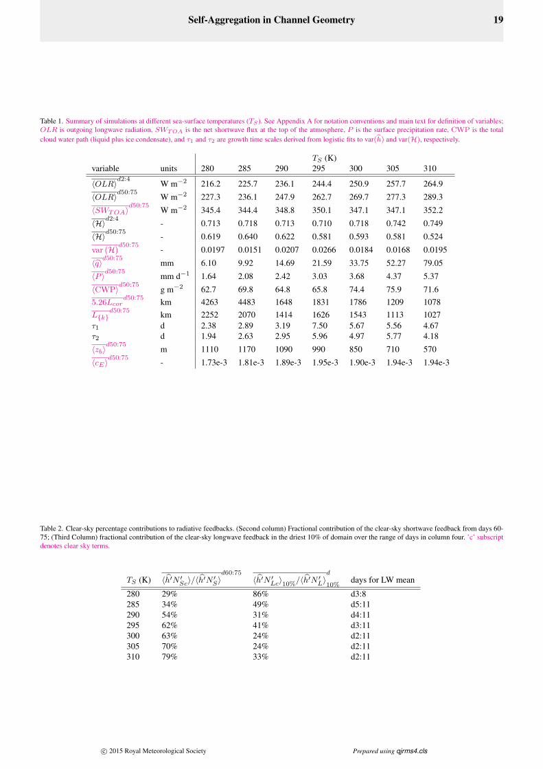
Self-Aggregation in Channel Geometry 19
Table 1. Summary of simulations at different sea-surface temperatures (TS ). See Appendix A for notation conventions and main text for definition of variables;OLR is outgoing longwave radiation, SWTOA is the net shortwave flux at the top of the atmosphere, P is the surface precipitation rate, CWP is the totalcloud water path (liquid plus ice condensate), and τ1 and τ2 are growth time scales derived from logistic fits to var(h) and var(H), respectively.
TS (K)variable units 280 285 290 295 300 305 310
〈OLR〉d2:4
W m−2 216.2 225.7 236.1 244.4 250.9 257.7 264.9
〈OLR〉d50:75
W m−2 227.3 236.1 247.9 262.7 269.7 277.3 289.3
〈SWTOA〉d50:75
W m−2 345.4 344.4 348.8 350.1 347.1 347.1 352.2
〈H〉d2:4
- 0.713 0.718 0.713 0.710 0.718 0.742 0.749
〈H〉d50:75
- 0.619 0.640 0.622 0.581 0.593 0.581 0.524
var (H)d50:75
- 0.0197 0.0151 0.0207 0.0266 0.0184 0.0168 0.0195
〈q〉d50:75
mm 6.10 9.92 14.69 21.59 33.75 52.27 79.05
〈P 〉d50:75
mm d−1 1.64 2.08 2.42 3.03 3.68 4.37 5.37
〈CWP〉d50:75
g m−2 62.7 69.8 64.8 65.8 74.4 75.9 71.65.26Lcor
d50:75 km 4263 4483 1648 1831 1786 1209 1078L{k}
d50:75 km 2252 2070 1414 1626 1543 1113 1027τ1 d 2.38 2.89 3.19 7.50 5.67 5.56 4.67τ2 d 1.94 2.63 2.95 5.96 4.97 5.77 4.18
〈zb〉d50:75
m 1110 1170 1090 990 850 710 570
〈cE〉d50:75
- 1.73e-3 1.81e-3 1.89e-3 1.95e-3 1.90e-3 1.94e-3 1.94e-3
Table 2. Clear-sky percentage contributions to radiative feedbacks. (Second column) Fractional contribution of the clear-sky shortwave feedback from days 60-75; (Third Column) fractional contribution of the clear-sky longwave feedback in the driest 10% of domain over the range of days in column four. ’c’ subscriptdenotes clear sky terms.
TS (K) 〈h′N ′Sc〉/〈h′N′S〉d60:75
〈h′N ′Lc〉10%/〈h′N ′L〉
d
10%days for LW mean
280 29% 86% d3:8285 34% 49% d5:11290 54% 31% d4:11295 62% 41% d3:11300 63% 24% d2:11305 70% 24% d2:11310 79% 33% d2:11
c© 2015 Royal Meteorological Society Prepared using qjrms4.cls

20 A. Wing and T. Cronin
(a) 280 K
Hovmuller Plots of Column Relative Humidity
02
46
81
01
2
(b) 285 K
02
46
81
01
2
(c) 290 K
02
46
81
01
2
(d) 295 K
Alo
ng
-Ch
an
ne
l D
ista
nce
, x (
10
3 k
m)
02
46
81
01
2
(e) 300 K
02
46
81
01
2
(f) 305 K
02
46
81
01
2
(g) 310 K
Time (days)0 10 20 30 40 50 60 70
02
46
81
01
2
0.1 0.2 0.3 0.4 0.5 0.6 0.7 0.8Column Relative Humidity, H
Figure 1. Hovmuller plot of column relative humidity, H (Equation 1), across themain set of simulations. Time runs left to right, and data are averaged over the shortcross-channel y-dimension. Subfigures (a)-(g) are for values of TS from 280-310K, in increments of 5 K, with temperature increasing downwards.
c© 2015 Royal Meteorological Society Prepared using qjrms4.cls

Self-Aggregation in Channel Geometry 21
〈Ti〉 (K)200 250 300
Pressure
(hPa)
100
200
300
400
500
600
700
800
900
1000
(a) Initial Temperature
280
285
290
295
300
305
310
〈T 〉d50:75
− 〈Ti〉 (K)
-10 0 10
100
200
300
400
500
600
700
800
900
1000
(b) Temperature Change
(〈q〉/〈q∗〉)d50:75
− (〈q〉/〈q∗〉)i
-0.4 -0.2 0 0.2
100
200
300
400
500
600
700
800
900
1000
(c) Relative Humidity Change
Figure 2. Domain average profiles of (a) initial temperature, and changes between the initial sounding and days 50-75 of each simulation for (b) temperature and (c)relative humidity. Colors indicate sea-surface temperature of the channel simulation, and 〈·〉 indicates the horizontal mean of a quantity.
c© 2015 Royal Meteorological Society Prepared using qjrms4.cls

22 A. Wing and T. Cronin
Time (days)10 20 30 40 50 60 70
(J/m
2)2
1011
1012
1013
1014
1015(a) Evolution of var(h)
280 (-- τ = 2.4d)285 (-- τ = 2.9d)290 (-- τ = 3.2d)295 (-- τ = 7.5d)300 (-- τ = 5.7d)305 (-- τ = 5.6d)310 (-- τ = 4.7d)
Time (days)10 20 30 40 50 60 70
0
0.005
0.01
0.015
0.02
0.025
0.03
0.035(b) Evolution of var(H)
280 (-- τ = 1.9d)285 (-- τ = 2.6d)290 (-- τ = 3.0d)295 (-- τ = 6.0d)300 (-- τ = 5.0d)305 (-- τ = 5.8d)310 (-- τ = 4.2d)
Figure 3. Evolution of (a): var(h) (J2/m4) and (b): var(H), in solid lines, andlogistic fits to each, in thin dashed lines, for the main set of simulations at differentvalues of TS . The vertical scale is (a) logarithmic, and (b) linear, and the legendindicates the initial e-folding growth time scale from each logistic fit.
c© 2015 Royal Meteorological Society Prepared using qjrms4.cls
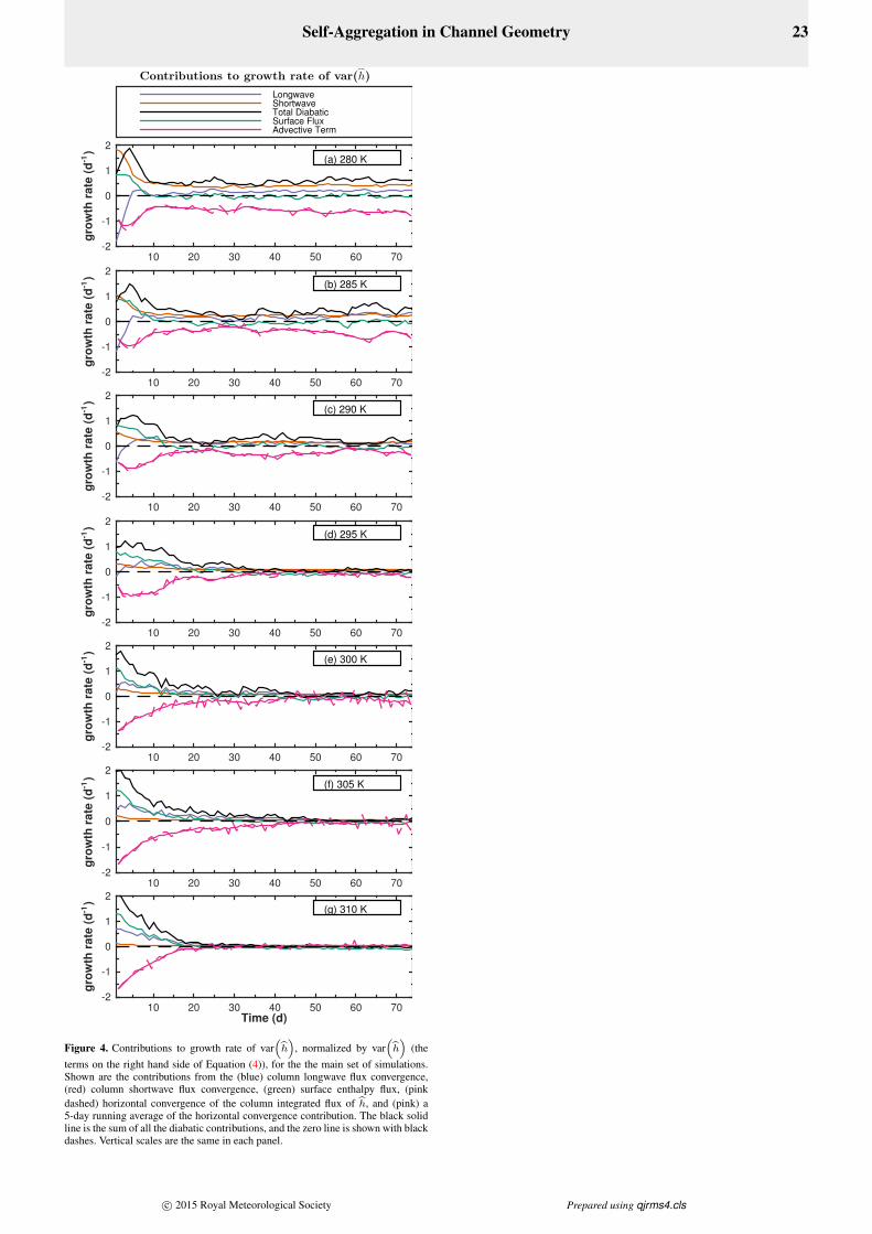
Self-Aggregation in Channel Geometry 23
10 20 30 40 50 60 70
gro
wth
ra
te (
d-1
)
-2
-1
0
1
2
10 20 30 40 50 60 70
gro
wth
ra
te (
d-1
)
-2
-1
0
1
2
10 20 30 40 50 60 70
gro
wth
ra
te (
d-1
)
-2
-1
0
1
2
10 20 30 40 50 60 70
gro
wth
ra
te (
d-1
)
-2
-1
0
1
2
10 20 30 40 50 60 70
gro
wth
ra
te (
d-1
)
-2
-1
0
1
2
10 20 30 40 50 60 70
gro
wth
ra
te (
d-1
)
-2
-1
0
1
2
Time (d)10 20 30 40 50 60 70
gro
wth
ra
te (
d-1
)
-2
-1
0
1
2
LongwaveShortwaveTotal DiabaticSurface FluxAdvective Term
Contributions to growth rate of var(h)
(a) 280 K
(b) 285 K
(c) 290 K
(d) 295 K
(e) 300 K
(f) 305 K
(g) 310 K
Figure 4. Contributions to growth rate of var(h)
, normalized by var(h)
(theterms on the right hand side of Equation (4)), for the the main set of simulations.Shown are the contributions from the (blue) column longwave flux convergence,(red) column shortwave flux convergence, (green) surface enthalpy flux, (pinkdashed) horizontal convergence of the column integrated flux of h, and (pink) a5-day running average of the horizontal convergence contribution. The black solidline is the sum of all the diabatic contributions, and the zero line is shown with blackdashes. Vertical scales are the same in each panel.
c© 2015 Royal Meteorological Society Prepared using qjrms4.cls

24 A. Wing and T. Cronin
10 20 30 40 50 60 70
gro
wth
ra
te (
d-1
)
-2
-1
0
1
2
10 20 30 40 50 60 70
gro
wth
ra
te (
d-1
)
-1.5
-1
-0.5
0
0.5
1
1.5
10 20 30 40 50 60 70
gro
wth
ra
te (
d-1
)
-1
-0.5
0
0.5
1
10 20 30 40 50 60 70
gro
wth
ra
te (
d-1
)
-0.2
0
0.2
0.4
0.6
10 20 30 40 50 60 70
gro
wth
ra
te (
d-1
)
-0.2
0
0.2
0.4
0.6
10 20 30 40 50 60 70
gro
wth
ra
te (
d-1
)
-0.2
0
0.2
0.4
0.6
0.8
Time (d)10 20 30 40 50 60 70
gro
wth
ra
te (
d-1
)
-0.2
0
0.2
0.4
0.6
0.8
LWLW-clearSWSW-clear
Contributions to growth rate of var(h)
(a) 280 K
(b) 285 K
(c) 290 K
(d) 295 K
(e) 300 K
(f) 305 K
(g) 310 K
Figure 5. Radiative contributions to growth rate of var(h)
, normalized by var(h)
(the second and third terms on the right hand side of Equation (4)), for the main setof simulations. Shown are the contributions from the (thick blue) column longwaveflux convergence, (thin bright blue) clear sky column longwave flux convergence,(thick red) column shortwave flux convergence, and (thin bright red) clear skycolumn shortwave flux convergence. The zero line is shown with black dashes.Vertical scales are different in each panel.
c© 2015 Royal Meteorological Society Prepared using qjrms4.cls

Self-Aggregation in Channel Geometry 25
Time (days)10 20 30 40 50 60 70
Correlation
Length
,L{k
}(k
m)
0
500
1000
1500
2000
2500
3000
3500
4000
4500
(a) Correlation length of precipitable water
Wavenumber, k (cycles/Lx)10
010
110
210
3PowerSpectralDensity
ofq,(φ
(k))
100
102
104
106
108
1010(b) Power spectra of precipitable water (d 50-75)
280
285
290
295
300
305
310
φ ∝ k−3
Figure 6. In (a), the evolution of correlation length of precipitable water (PW),using the metric L{k}, for the main set of simulations. Averages over days 50-75are given in Table 1. In (b), the power spectra of PW, averaged over days 50-75; theblack dashed line indicates the slope of a k−3 spectrum.
c© 2015 Royal Meteorological Society Prepared using qjrms4.cls

26 A. Wing and T. Cronin
Remoistening length scale, LM (km)0 100 200 300 400 500 600 700
PW
correlation
length
,L{k
}(k
m)
0
500
1000
1500
2000
2500
280 K
285 K
290 K
295 K
300 K
305 K
310 K
Figure 7. Precipitable water (PW) correlation length, L{k}, and remoisteninglength scale LM = zb/cE , diagnosed from the main set of simulations (filledcircles), and from a set of simulations with an alternative radiation scheme (RRTM,open circles) at different sea-surface temperatures (different colors). The values arefrom averages over the final 25 days of each simulation. The boundary layer heightzb is calculated as the lower-tropospheric maximum of a three-point quadratic fitof ∂2θv/∂z
2 in the unsaturated environment, and cE is the moisture exchangecoefficient from Table 1. The dashed line shows the best-fit line through the filledcircles and the origin, given by L{k} = 3.16LM ; the correlation coefficient forthis fit is R2=0.8.
c© 2015 Royal Meteorological Society Prepared using qjrms4.cls

Self-Aggregation in Channel Geometry 27
σcldd50:75
− σcldd2:4
-0.1 -0.05 0 0.05 0.1
Pressure
(hPa)
100
200
300
400
500
600
700
800
900
1000
(a) Cloud fraction change
280
285
290
295
300
305
310
qc,ld50:75
− qc,ld2:4 (mg/kg)
-5 0 5 10
100
200
300
400
500
600
700
800
900
1000
(b) Liquid Condensate Change
qc,id50:75
− qc,id2:4 (mg/kg)
-10 -5 0 5
100
200
300
400
500
600
700
800
900
1000
(c) Solid Condensate Change
Figure 8. Domain average profiles of change in (a) cloud fraction, (b) liquid condensate qc,l (c) and solid condensate qc,i, between days 2-4 and days 50-75. Colorsindicate sea-surface temperature of the channel simulation, and an overbar indicates a mean over the time range indicated.
c© 2015 Royal Meteorological Society Prepared using qjrms4.cls
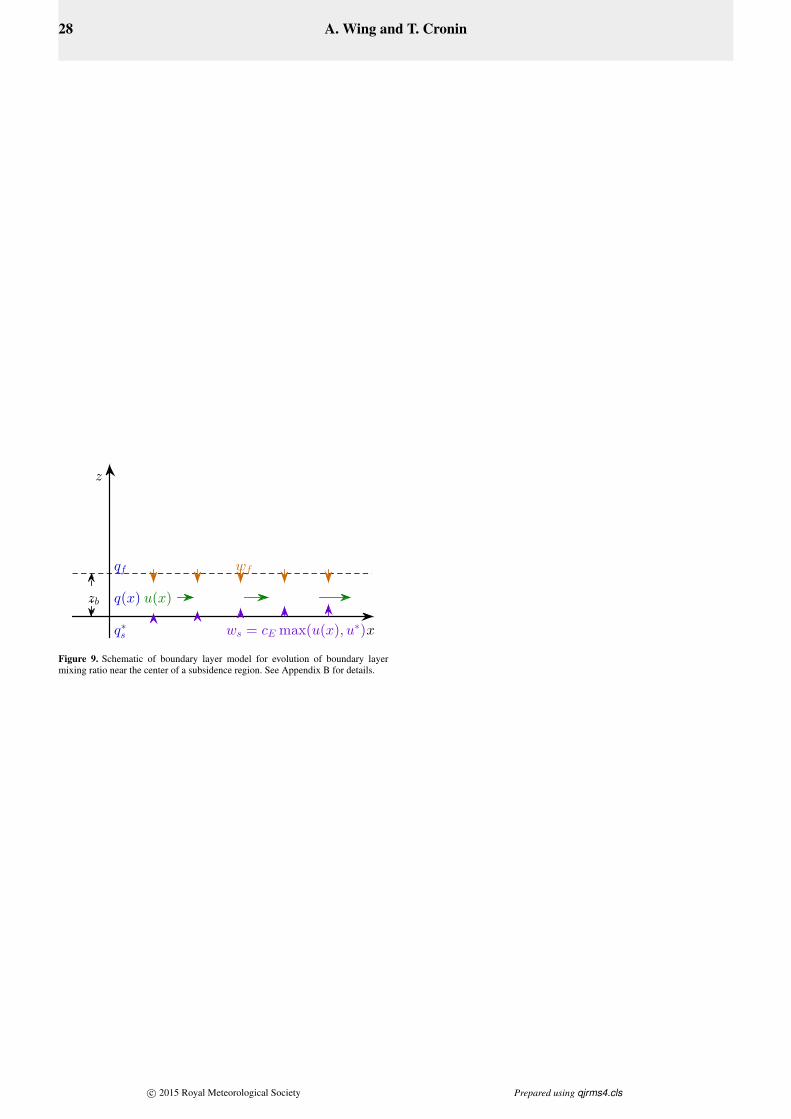
28 A. Wing and T. Cronin
x
z
zb q(x)
q∗s
qf
u(x)
wf
ws = cE max(u(x), u∗)
Figure 9. Schematic of boundary layer model for evolution of boundary layermixing ratio near the center of a subsidence region. See Appendix B for details.
c© 2015 Royal Meteorological Society Prepared using qjrms4.cls

Self-Aggregation in Channel Geometry 29
Nondimensional length, x = x/LM
0 1 2 3 4 5Nondim
ensionalmixingratio,q=
q/q∗ s
0
0.1
0.2
0.3
0.4
0.5
0.6
0.7
0.8
0.9
1
(m, a) = (0, 0)
(m, a) = (0.25, 0)
(m, a) = (0.5, 0)
(m, a) = (0.25, 0.1)
(m, a) = (0.25, 0.3)
(m, a) = (0.25, 1)
(m, a) = (0.25, 0.3); polar
Figure 10. Nondimensional mixing ratio plotted as a function of nondimensionallength for the idealized slab boundary layer model, based on (12), (13), and (14).
c© 2015 Royal Meteorological Society Prepared using qjrms4.cls