self-adjointness and the renormalization of singular potentials · 2008-10-08 · self-adjointness...
TRANSCRIPT
Self-Adjointness and the
Renormalization of Singular Potentials
Sarang GopalakrishnanAdvisor: Professor William Loinaz
Submitted to the Department of Physics of Amherst College inpartial fulfillment of the requirements for the degree of Bachelor
of Arts with Honors.
Submitted April 24, 2006
Abstract
Schrodinger operators with very singular potentials fail to produce reasonable spec-
tra, because the usual boundary conditions are insufficient to make them self-adjoint.
If one regularizes a singular potential at a length ε, the bound state energies diverge
as ε → 0. A meaningful spectrum can be restored by picking a self-adjoint exten-
sion of the operator, by renormalizing the theory, or by allowing nonunitary time
evolution. We show that renormalizations of the 1/r2 potential fall into two classes:
those that are asymptotically equivalent to self-adjoint extensions, and those that
reduce to treatments of delta functions. We also apply the apparatus of self-adjoint
extensions and renormalization to clarify aspects of anomalous symmetry breaking,
supersymmetric quantum mechanics, and one-dimensional quantum mechanics.

Lines composed upon readinga thesis abstract by S. Gopalakrishnan
Think a moment, dear reader, of that long-legged fly,
The sprung meniscus underfoot,
And what asymptotes invisible to well-trained eyes
Still break the surface at its root.
How a singular potential picks tight-bounded energy
Apart till it no longer recognizes
Its own mirrored face, its extensions, or symmetry;
Unless one cautiously renormalizes.
You have tried in these pensive pages to show the stuff
Such theory’s made of, its quiddity
When logic is applied to the diamond rough,
And quantum notes ring purely.
May Apollo’s clarity pierce through your reasoning
And self-adjointed truth and fact
Elevate your thought to that sense so pleasing
When truth recovers nature’s pact.
Jesse McCarthy
Acknowledgments
First, I would like to thank my advisor, Professor Loinaz, for suggesting an interesting
topic, guiding me through the literature, ploughing through quantities of papers that
had nothing to do with his research, contributing his insight and his sharp nose for
problems, catching several errors in drafts, and always being there—literally there,
in his office—when I needed his advice. I would also like to thank him for the long,
entertaining, and often instructive conversations we have had every week this year.
I am indebted to my readers, Professors Hilborn and Zajonc, and to Professor
Friedman, for their corrections.
Others I wish to thank are Professor Jagannathan, for reading a draft of my thesis,
and for providing me with excellent suggestions, food, and drink; the Department of
Physics, for their support over the years; Professors Benedetto and Call, for teaching
me real analysis; Professor Griffiths of Reed College, and Andrew Essin of the Uni-
versity of California, Berkeley, for access to Mr. Essin’s undergraduate thesis; the
Office of the Dean of Faculty, for the Mellon Internship that supported my research
last summer; Jesse McCarthy, for his dedicatory poem, which is the high point of
this thesis; Kit Wallach, for her wonderful “dramatic proofreading” of some chapters;
Mike Foss-Feig, Dave Schaich, Dave Stein, Eduardo Higino da Silva Neto, Dave Got-
tlieb, Daisuke O, and others, for their ruinous influence on my lifestyle and morals;
Liz Hunt, who was there to comfort us when we failed the comps; and, finally, my
professors, roommates, friends, and parents for their good humor, which ameliorated
a predictably difficult year.
Sarang Gopalakrishnan
1
Contents
1 Delta Functions 15
1.1 Effective Field Theories . . . . . . . . . . . . . . . . . . . . . . . . . . 15
1.2 δ(x) in One Dimension . . . . . . . . . . . . . . . . . . . . . . . . . . 16
1.3 The 2D Schrodinger Equation . . . . . . . . . . . . . . . . . . . . . . 19
1.4 The 2D Delta Function . . . . . . . . . . . . . . . . . . . . . . . . . . 21
1.5 Renormalizing the 2D Delta Function . . . . . . . . . . . . . . . . . . 22
1.6 Scale Invariance and the Anomaly . . . . . . . . . . . . . . . . . . . . 25
1.7 The 2D Delta Function as Limit of Rings . . . . . . . . . . . . . . . . 27
1.8 The 3D Delta Function . . . . . . . . . . . . . . . . . . . . . . . . . . 28
1.9 More Dimensions, etc. . . . . . . . . . . . . . . . . . . . . . . . . . . 29
1.10 The δ′(x) Potential . . . . . . . . . . . . . . . . . . . . . . . . . . . . 29
2 Self-Adjoint Extensions 33
2.1 Hilbert Space . . . . . . . . . . . . . . . . . . . . . . . . . . . . . . . 33
2.2 Linear Operators and their Domains . . . . . . . . . . . . . . . . . . 38
2.3 Self-Adjoint Extensions . . . . . . . . . . . . . . . . . . . . . . . . . . 41
2.4 The Physics of Self-Adjoint Extensions . . . . . . . . . . . . . . . . . 44
2.5 Boundedness and the Friedrichs Extension . . . . . . . . . . . . . . . 53
2.6 Rigged Hilbert Space Formalism . . . . . . . . . . . . . . . . . . . . . 54
3 Singular Potentials 57
3.1 The Inverse Square Potential . . . . . . . . . . . . . . . . . . . . . . . 57
3.2 Strongly Repulsive Regime (λ ≥ 34, ζ ≥ 1
2) . . . . . . . . . . . . . . . 58
3.3 Weak Regime (−14< λ < 3
4, |ζ| < 1
2) . . . . . . . . . . . . . . . . . . . 59
3.4 Critical Value (λ = −14) . . . . . . . . . . . . . . . . . . . . . . . . . 61
3.5 Strongly Attractive Regime (λ < −14) . . . . . . . . . . . . . . . . . . 62
3.6 Singularity vs. Anomaly . . . . . . . . . . . . . . . . . . . . . . . . . 64
2
3.7 Non-Friedrichs Extensions of the 1/r2 Potential . . . . . . . . . . . . 67
3.7.1 One Dimension . . . . . . . . . . . . . . . . . . . . . . . . . . 67
3.7.2 Two Dimensions . . . . . . . . . . . . . . . . . . . . . . . . . 70
3.7.3 Three Dimensions . . . . . . . . . . . . . . . . . . . . . . . . . 72
3.8 Infinite Well with an Inverse Square Term . . . . . . . . . . . . . . . 73
3.9 The Classical Limit . . . . . . . . . . . . . . . . . . . . . . . . . . . . 74
4 Global Renormalization 76
4.1 Hardcore Cutoff . . . . . . . . . . . . . . . . . . . . . . . . . . . . . . 76
4.2 Square Well Cutoff . . . . . . . . . . . . . . . . . . . . . . . . . . . . 78
4.3 Dimensional Regularization . . . . . . . . . . . . . . . . . . . . . . . 79
4.4 Schwartz’s Way . . . . . . . . . . . . . . . . . . . . . . . . . . . . . . 79
4.5 Summary . . . . . . . . . . . . . . . . . . . . . . . . . . . . . . . . . 84
5 Limit Cycles 85
5.1 Running Square Well . . . . . . . . . . . . . . . . . . . . . . . . . . . 85
5.2 Flows, Revisited . . . . . . . . . . . . . . . . . . . . . . . . . . . . . . 88
5.3 Running δ-function . . . . . . . . . . . . . . . . . . . . . . . . . . . . 89
5.4 The 1/r4 Potential . . . . . . . . . . . . . . . . . . . . . . . . . . . . 90
5.5 Scaling Properties . . . . . . . . . . . . . . . . . . . . . . . . . . . . . 92
5.6 Consistency with Chapter 4 . . . . . . . . . . . . . . . . . . . . . . . 96
5.7 RG Treatment of Weak Coupling . . . . . . . . . . . . . . . . . . . . 98
5.7.1 What Sort of Physics? . . . . . . . . . . . . . . . . . . . . . . 98
5.7.2 Critical Coupling . . . . . . . . . . . . . . . . . . . . . . . . . 101
5.7.3 Two Dimensions . . . . . . . . . . . . . . . . . . . . . . . . . 102
5.7.4 Conclusions . . . . . . . . . . . . . . . . . . . . . . . . . . . . 102
6 Fall to the Center 103
6.1 Contraction Semigroups . . . . . . . . . . . . . . . . . . . . . . . . . 104
6.2 Dissipative Particle on Half-Line . . . . . . . . . . . . . . . . . . . . . 106
6.3 Absorption by a 1/r2 potential . . . . . . . . . . . . . . . . . . . . . . 107
6.4 Experimental Realization . . . . . . . . . . . . . . . . . . . . . . . . . 111
7 Klauder Phenomena and Universality 112
7.1 Self-Adjoint Extensions and Klauder Phenomena . . . . . . . . . . . 112
7.2 Examples . . . . . . . . . . . . . . . . . . . . . . . . . . . . . . . . . 114
3
7.2.1 1/r2 in the Plane . . . . . . . . . . . . . . . . . . . . . . . . . 114
7.2.2 1/x2 on the Half-Line . . . . . . . . . . . . . . . . . . . . . . . 115
7.2.3 Self-Adjoint Extensions . . . . . . . . . . . . . . . . . . . . . . 116
7.3 Nonanalyticity . . . . . . . . . . . . . . . . . . . . . . . . . . . . . . . 118
7.4 Universality . . . . . . . . . . . . . . . . . . . . . . . . . . . . . . . . 119
7.4.1 Review of 3D Scattering . . . . . . . . . . . . . . . . . . . . . 119
7.4.2 Bound States and Resonances . . . . . . . . . . . . . . . . . . 120
7.4.3 Three-Body Scattering . . . . . . . . . . . . . . . . . . . . . . 121
7.4.4 The Efimov Effect . . . . . . . . . . . . . . . . . . . . . . . . 121
7.4.5 Consequences and Experimental Realization . . . . . . . . . . 122
8 The One-Dimensional Hydrogen Atom 123
8.1 The Trouble with 1D Quantum Mechanics . . . . . . . . . . . . . . . 124
8.2 Free Particle on R− 0 . . . . . . . . . . . . . . . . . . . . . . . . . 125
8.2.1 The General Solution . . . . . . . . . . . . . . . . . . . . . . . 125
8.2.2 The Disconnected Family . . . . . . . . . . . . . . . . . . . . 127
8.2.3 The Bipolar Family . . . . . . . . . . . . . . . . . . . . . . . . 128
8.2.4 The Degenerate Family . . . . . . . . . . . . . . . . . . . . . . 128
8.2.5 The 1D Delta Function, Done Differently . . . . . . . . . . . . 129
8.3 The 1D Coulomb Potential . . . . . . . . . . . . . . . . . . . . . . . . 130
8.3.1 Why We Need the Whole Family . . . . . . . . . . . . . . . . 130
8.3.2 Solving the Equation . . . . . . . . . . . . . . . . . . . . . . . 131
8.3.3 The Boundary Condition . . . . . . . . . . . . . . . . . . . . . 132
8.4 Renormalization of the 1/|x| Potential . . . . . . . . . . . . . . . . . 134
8.4.1 Loudon’s Regularization . . . . . . . . . . . . . . . . . . . . . 134
8.4.2 Chapter 5 Renormalization . . . . . . . . . . . . . . . . . . . . 134
8.4.3 The Quantization Condition . . . . . . . . . . . . . . . . . . . 135
8.4.4 Summary . . . . . . . . . . . . . . . . . . . . . . . . . . . . . 135
8.5 Other 1D Potentials . . . . . . . . . . . . . . . . . . . . . . . . . . . 137
8.5.1 The Strong 1/x2 Potential . . . . . . . . . . . . . . . . . . . . 137
8.5.2 Singular SUSY . . . . . . . . . . . . . . . . . . . . . . . . . . 137
9 Issues of Symmetry 139
9.1 Anomaly Revisited . . . . . . . . . . . . . . . . . . . . . . . . . . . . 139
9.2 A Ladder Operator? . . . . . . . . . . . . . . . . . . . . . . . . . . . 143
4
9.3 Supersymmetry . . . . . . . . . . . . . . . . . . . . . . . . . . . . . . 144
9.3.1 Supersymmetric Oscillator on the Half-Line . . . . . . . . . . 146
9.3.2 The x2 + 1/x2 Potential . . . . . . . . . . . . . . . . . . . . . 147
9.4 Virasoro Algebra of the 1/x2 Potential . . . . . . . . . . . . . . . . . 149
10 Summary and Applications 151
10.1 Singular Potentials in Physics . . . . . . . . . . . . . . . . . . . . . . 153
10.1.1 The Relativistic Coulomb Problem . . . . . . . . . . . . . . . 153
10.1.2 Solvable Models with Singular Interactions . . . . . . . . . . . 154
10.1.3 Dipoles and Black Holes . . . . . . . . . . . . . . . . . . . . . 154
10.2 Executive Summary . . . . . . . . . . . . . . . . . . . . . . . . . . . . 154
A Deriving the Duality Transformation 155
5
Introduction
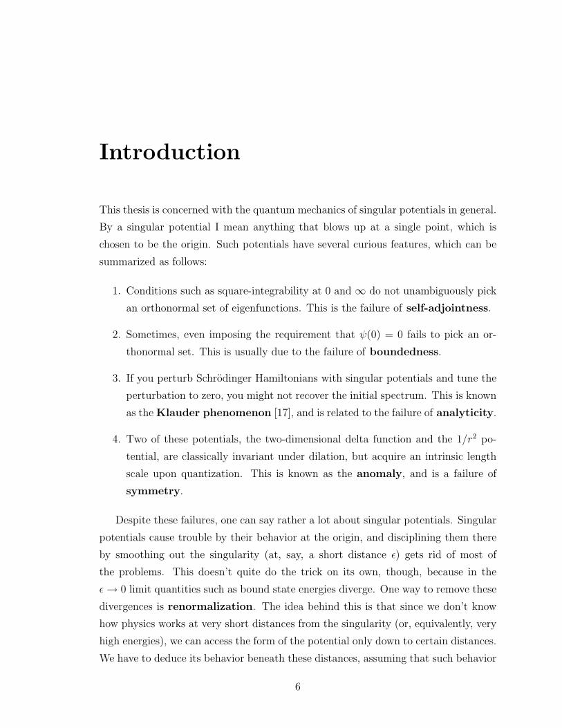
This thesis is concerned with the quantum mechanics of singular potentials in general.
By a singular potential I mean anything that blows up at a single point, which is
chosen to be the origin. Such potentials have several curious features, which can be
summarized as follows:
1. Conditions such as square-integrability at 0 and ∞ do not unambiguously pick
an orthonormal set of eigenfunctions. This is the failure of self-adjointness.
2. Sometimes, even imposing the requirement that ψ(0) = 0 fails to pick an or-
thonormal set. This is usually due to the failure of boundedness.
3. If you perturb Schrodinger Hamiltonians with singular potentials and tune the
perturbation to zero, you might not recover the initial spectrum. This is known
as the Klauder phenomenon [17], and is related to the failure of analyticity.
4. Two of these potentials, the two-dimensional delta function and the 1/r2 po-
tential, are classically invariant under dilation, but acquire an intrinsic length
scale upon quantization. This is known as the anomaly, and is a failure of
symmetry.
Despite these failures, one can say rather a lot about singular potentials. Singular
potentials cause trouble by their behavior at the origin, and disciplining them there
by smoothing out the singularity (at, say, a short distance ε) gets rid of most of
the problems. This doesn’t quite do the trick on its own, though, because in the
ε→ 0 limit quantities such as bound state energies diverge. One way to remove these
divergences is renormalization. The idea behind this is that since we don’t know
how physics works at very short distances from the singularity (or, equivalently, very
high energies), we can access the form of the potential only down to certain distances.
We have to deduce its behavior beneath these distances, assuming that such behavior
6
is finite and sensible, from some experimentally observed quantity like a bound state
or a scattering phase shift. Of course, given a bound state energy and a description
of long-distance behavior, there are infinitely many possible theories of short-distance
physics. The remarkable thing about renormalization is that all the theories that have
a bound state energy at E give the same values for all other low-energy observables.
That is, with the addition of one arbitrary experimental parameter, we can predict
all low-energy properties exactly.
There is an entirely different way to go about making these theories sensible,
which is to fix the failure of self-adjointness. In practice, this works by specifying
a bound state and deducing the rest of the spectrum from the requirement that
all other eigenstates be orthogonal to it. For low-energy observables this technique
produces exactly the same results as renormalization, and is mathematically more
rigorous. The trouble with renormalization is that it’s hard to prove something must
be true of all imaginable short-distance physics; however, requiring that the renor-
malized theory should coincide with a self-adjoint extension fixes this, because we
have a much better handle on the self-adjoint extensions of a Hamiltonian. We con-
sider the relation between renormalization and self-adjoint extensions in the context
of singular potentials—mostly delta functions and 1/r2 potentials—in the first five
chapters. Chapter 1 is about delta functions, Chapter 2 introduces self-adjoint exten-
sions, Chapter 3 introduces singular potentials and treats them with the apparatus
of Chapter 2, and Chapter 4 introduces various renormalization schemes. Chapter
5 discusses the renormalization group, a powerful way to study the behavior of
physical theories at various length scales.
The reason we like self-adjoint extensions—that they conserve probability—is
sometimes a limitation. Suppose we are looking at a system where a particle moving
in a singular potential falls into the singularity and gets absorbed: what then? This
question is of particular importance because a recent experiment [23] with cold atoms
moving in a 1/r2 potential noticed that some of the atoms were absorbed. Chapter 6
discusses nonunitary extensions of quantum mechanics that deal with such situations.
Chapter 7 is somewhat heterogeneous; it is about Klauder phenomena, non-
analyticity, and resonance phenomena. The link between resonance and Klauder
phenomena is that they are both universal. Klauder phenomena are independent of
what the original perturbation was, and resonant interactions in quantum mechanics
are the same for all potentials. Singular potentials are connected to resonance phe-
7
nomena by the Efimov effect [27]. In a system of three identical bodies for which all
the two-body interactions are tuned to resonance, the three-body Schrodinger equa-
tion obeys a 1/r2 force law, and has infinitely many three-body bound states. This
effect too has recently been observed experimentally [39].
Chapter 8 discusses the one-dimensional hydrogen atom and other issues in one-
dimensional quantum mechanics that arise from the fact that R−0 is disconnected.
Chapter 9 discusses the symmetry structures, broken and otherwise, of the 1/r2 prob-
lem. Chapter 10 summarizes everything and briefly discusses physical applications of
singular potentials.
Who Did What
Most of the key ideas in the first six chapters are not mine. The exception is the
explanation of the relationship between the very different spectra of the renormaliza-
tion schemes of Chapter 4 and Chapter 5. The treatment of self-adjoint extensions
for singular potentials is, however, more explicit and detailed than elsewhere in the
literature, and as far as I know this is the first detailed treatment of scattering observ-
ables in terms of self-adjoint extensions, and the first explicit treatment of nonunitary
extensions as complex boundary conditions within the deficiency subspace framework.
I’m not aware of any previous work on the universality of Klauder phenomena;
the idea isn’t a deep one, but it is relevant to the renormalization schemes studied
in Chapter 4. There have been several previous treatments of the one-dimensional
hydrogen atom, but as far as I know, mine is the first to apply ideas from renormal-
ization to the problem, or to characterize the family of extensions in terms of δ and
δ′ counterterms. My treatment of the two-parameter family was developed indepen-
dently of Ref. [95], but they had the key idea before I did. (On the other hand, my
treatment of the x2 +1/x2 potential follows theirs quite closely.) The approach to the
anomaly in terms of self-adjointness and finite dilations is, again, relatively obvious,
but it hasn’t been done in the literature. My approach to the SO(2, 1) algebra was
different from Jackiw’s [41]; for consistency with the rest of this thesis, I tried to
reduce it to a time-independent symmetry, but was unable to get very far.
8
History of Previous Literature
There are, roughly speaking, three classes of singular potentials: mildly singular
(solvable with regular QM), singular (problematic, but with ground states), and very
singular (without a ground state). As the literature is considerable and I discuss most
of the important ideas later, I have left my history skeletal, to avoid overwhelming the
sequence of discoveries with irrelevant detail. For the most part, I have ignored ex-
clusively pedagogical articles. I have left the history of the one-dimensional Coulomb
problem, which is somewhat disjoint from this sequence, to the chapter on it.
Early Work
The first important paper on singular potentials was K.M. Case’s treatment in 1950
[1]. Previously, the nonsingular—repulsive or weakly attractive—regimes had been
treated by Mott and Massey (1933)[3] and by Titchmarsh (1946)[2]. The operator
theory behind quantum mechanics had been developed in the 1930s by John von
Neumann [4], Marshall Stone, and various others; Stone’s monograph, Linear Trans-
formations in Hilbert Space (1932) [5], is a standard reference in the literature. The
strongly attractive (very singular) regime of the 1/r2 potential is dismissed as un-
physical by the early writers; however, as Case notes, the Klein-Gordon and Dirac
equations for the hydrogen atom have similar singularities.
Case shows that the strongly singular regime of the 1/r2 potential, treated naively,
has a continuum of bound states. This implies that the operator is not Hermitian,
but Case restricts the domain of definition of H to restore Hermeticity, and finds a
point spectrum of bound states going all the way down to −∞. These restrictions
are Hermitian, but depend on an arbitrary phase parameter. He also shows that
potentials more singular than 1/r2 have similar properties. A more specific early
treatment of the 1/r2 case is due to Meetz (1964) [6], who discusses self-adjoint
extensions explicitly (though the idea was implicit in Case’s work). Meetz notes that
there is a singular regime to this potential in addition to the very singular regime;
this corresponds to the failure of self-adjointness for weakly repulsive and weakly
attractive 1/r2 potentials. Narnhofer (1974) [7] gives a detailed expository treatment
of this problem, and suggests that contraction semigroups might be helpful. She
shows that the “natural” continuation of the “natural” self-adjoint extension into the
very singular regime is nonunitary.
9

Vogt and Wannier (1954) [8] give a nonunitary solution to the 1/r4 problem, and
preen themselves (rather ironically) about having avoided Case’s “involved” math-
ematics. Nelson (1963) [9] arrives at a nonunitary result for the 1/r2 case by ana-
lytically continuing the functional integral; he basically hits the same nonanalyticity
that Narnhofer does fifteen years later.
The 1967 review article by Frank, Land, and Spector [11] summarizes much of
the early work on these potentials, and also discusses applications of very singular
potentials. A lot of this work is on approximation schemes and applications. Spector’s
(1964) [12] analytic solution of the 1/r4 potential is an exception; unfortunately, it is
not a very easy solution to use. A particularly important application is the Calogero-
Sutherland model (1969) [13], which describes N bosons interacting with pairwise
inverse-square potentials.
Self-Adjointness of Singular Potentials
The failure of self-adjointness at λ < 34
seems to have already been familiar to math-
ematicians as an example of Weyl’s limit-point/limit-circle theorem (1910); it is re-
ferred to quite casually in Simon’s 1974 paper on self-adjointness [14]. The strictly
mathematical literature on when Schrodinger operators are self-adjoint is huge, but
Simon’s “Review of Schrodinger operators in the 20th Century” (2000) [15] is a help-
ful guide, as is Vol. 2 of Reed and Simon’s book on Methods of Modern Mathematical
Physics [75]. Of more recent work, the most relevant papers are two papers by Tsutsui
et al [95], [96] on one-dimensional quantum mechanics, and Falomir’s discussion [92]
of supersymmetry and singular potentials. An independent source of mathematical
interest was Klauder’s (1973) study of Klauder phenomena [17].
Nonunitary Solutions
The term fall to the center was first applied to singular potentials by Landau
and Lifschitz in their quantum mechanics text (1958) [18], where the strong-coupling
regime is compared with the classical situation, for which the particle’s trajectory is
defined only for a finite time. This comparison between classical completeness (i.e.
having a solution for all time) and self-adjointness is explored rigorously in Reed and
Simon vol. II [75], and makes its way into the pedagogical literature with an AJP
article by Zhu and Klauder [19] on the “Classical Symptoms of Quantum Illnesses”
(1993).
10

Non-self-adjoint extensions of singular potentials are explored in some more detail
by Perelomov and Popov (1970) [20] and by Alliluev (1971) [21], using methods that
are equivalent to Nelson’s. The mathematical side of the semigroup theory had been
worked out previously by Hille, Yosida, Kato, Trotter, etc.; a classic text is Functional
Analysis and Semigroups by Hille and Phillips [10]. In 1979, Radin [22] observed
that Nelson’s nonunitary time-evolution operator could be written as an average over
the unitary operators corresponding to all the self-adjoint extensions. (This is not
especially shocking, since e.g. eiθ and e−iθ, which are unitary, average to cos θ, which
is not.)
This work found some physical application in 1998, when Denschlag et al experi-
mentally realized an attractive 1/r2 potential by scattering cold neutral atoms off a
charged wire [23], and found that the atoms were absorbed. This result was treated
variously by Audretsch et al (1999) [24] and by Bawin and Coon (2001) [25], who use
Radin’s result to “justify” the cross-section.
A related, and intriguing, result is Bawin’s proof (1977) [26] that spectra very
different from Case’s could be obtained by redefining the inner product.
Effective Field Theories
In his famous paper of 1971 [27], Vitaly Efimov noted that in certain regimes, the
three-body problem reduces to that of particles moving in an effective 1/r2 potential,
and this produces a large number of bound states. (There is a huge literature on
the Efimov effect, which we will not attempt to cover.) Efimov’s result made it
desirable to apply ideas from the effective field theory (EFT) program to the 1/r2
potential, and thus prompted the treatments of Bedaque, Hammer, and Van Kolck
(1999) [29], and of Beane et al (2001) [30]. The treatment in [29] uses field theoretic
methods, while [30] constructs an effective theory of the interaction by cutting off
the potential at short distances by a square well. In their paper, Beane et al find
that the renormalization group flow equations of the 1/r2 potential have two
sorts of solutions—continuous paths that don’t go all the way to the origin, and
log-periodic paths that represent limit cycles. Beane et al treat singular potentials
quite generally; more specific treatments of the 1/r2 case are done by Bawin and Coon
(2003) [31], who solve the RG flow equations analytically, and Braaten and Phillips
(2004) [32], who discovered that using a δ-function ring cutoff instead of a square well
cutoff forces one to choose the limit cycle. The idea of limit cycles in this context,
11
and a lot of the conceptual basis for this work, is due to Kenneth Wilson’s (1971)
work on the renormalization group [34].1 The specific method that these authors use
was suggested by Lepage(1997) [33]. Recently, Alberg, Bawin, and Brau (2005) [36]
used a similar approach to treat the 1/r4 potential; however, they did not consider
δ-function regularizations.
After decades of strenuous effort, the Efimov effect was finally demonstrated in
the laboratory this year with cold atoms [39]. Another recent milestone in that area
was the long review article on universality by Braaten and Hammer [40], which uses
the same language as above-mentioned papers.
In general, solutions found by these methods are unitary and involve spectra with
arbitrarily many bound states.
Algebraic Structures
Anomalies are cases where a classical symmetry is broken by quantization. They are
pervasive and very important in quantum field theory. It has been known for some
time that the 1/r2 and δ2(r) potentials are examples of the anomaly in nonrelativistic
quantum mechanics. Jackiw [41] looks at the broken SO(2,1) algebra associated with
both potentials in his 1991 paper on delta function potentials; this is taken up in more
detail by Camblong and Ordonez (2003, 2005) [44], [43], who also discuss various
applications of conformal QM. A somewhat different algebraic treatment is given by
Birmingham, Gupta, and Sen (2001) [42], who study the representation theory of the
Virasoro algebra underlying this problem.
Renormalizing the Coupling
Gupta and Rajeev (1993) [52] renormalized the long-distance coupling of the very
singular 1/r2 potential, and got a renormalized spectrum with just one bound state,
which looked essentially the same as that of the δ2 potential. Their result was worked
out in just one dimension, but it was later generalized by Camblong et al (2000) [45],
who also got the same answer by dimensional regularization [47], [48]. Camblong’s
result was reworked in an AJP article by Coon and Holstein (2002) [46], and later by
Essin and Griffiths (2006) [51]. This approach to the potential also constituted the
bulk of Essin’s undergraduate thesis (2003).
1Limit cycles were, however, borrowed from dynamics, where they actually make sense.
12
Notes to the Reader
Sequence
This thesis was written to be read in sequence, but it needn’t be. The first three
chapters are essential context for chapters 4-7 and 9. Chapter 5 uses the results
of Chapter 4 but not the details. Chapter 6 is independent of Chapters 4 and 5,
and may be skipped without loss of continuity. Chapter 7 deals with issues raised
in Chapters 4 and 5, so it should be read after them. Chapter 8 uses the entire
apparatus developed thus far, but is independent of Chapters 3 and 4. Chapter 9 is
independent of Chapters 4-8. In later chapters I sometimes use the terms “Chapter 4”
and “Chapter 5” renormalization to refer, respectively, to schemes that renormalize
the long-distance coupling and schemes that don’t.
The bulk of original work is in the later sections of Chapters 3 and 5, and all of
Chapters 7 and 8.
Units, Dimensions, Notation
I have set ~ = 2m = 1. Since the first term in Schrodinger’s equation is then just
−∇2ψ, which has dimensions [length]−2[ψ], consistency requires that V and E have
dimensions of [length]−2. This turns out to be an immense convenience, though it
might take some getting used to.
More irritatingly, I suppose, I have freely used the identity log kr = log k + log r
even if k and r have dimensions. The departure from dimensional consistency might
make the equations harder to check, but is standard in the literature and makes
several equations a lot tidier. The reader is requested to imagine, should s/he wish,
that there are ghostly η’s and η−1’s hovering by the dimensional quantities and just
canceling them out.
References of the form AS 1.1.1 are to identities in Abramowitz and Stegun [58].
Finally, I should comment on my inner products, which are always (ψ1, ψ2) and
never 〈ψ1|ψ2〉. In Dirac notation, one is used to thinking that a Hermitian operator
A in the middle of a bracket
〈ψ|A|φ〉
might be acting either to its left or to its right, depending solely on the reader’s
whim. When dealing with issues of self-adjointness, it is extremely important to know
13

whether one is operating on the bra or the ket, and the mathematicians’ notation,
which forces us to pick either (Aψ, φ) or (ψ,Aφ), has the merit of being entirely
unambiguous about this.
14

Chapter 1
Delta Functions
Potentials shaped like Dirac delta functions are useful in the study of singular po-
tentials for several reasons, most of which will be left to subsequent chapters. There
are two general strands to the answer; the first is that delta functions are easy to
solve, and the second is that they are conceptually important to the effective field
theory (EFT) program, which I’ll discuss now. The two dimensional delta function
is independently interesting because it lacks an explicit scale; along with the 1/r2
potential, it is an example of the “anomaly” in quantum mechanics.
1.1 Effective Field Theories
The idea behind effective field theories is that you can describe the low-energy, long-
distance behavior of a theory very powerfully by an “effective theory” without know-
ing much about its high-energy, short-distance behavior. This generally requires
renormalization, which casts our effective theory entirely in terms of low-energy
experimental observables; renormalization becomes necessary when our effective the-
ory has divergences due to high-energy behavior (where the approximation breaks
down), but isn’t always required. In the case of the hydrogen atom, for instance, the
effective model of a 1/r potential is not valid to arbitrarily short distances, but the
eigenvalues still converge, and so we needn’t worry about short-distance behavior at
all. On the other hand, some theories cannot be renormalized because their behavior
at all energies is strongly affected by the details of high-energy processes—so different
parameterizations of high-energy behavior lead to radically different theories.
Delta function potentials are frequently used in effective theories as a simple char-
15
acterization of high-energy physics, because their action is entirely local, and they
are relatively easy to do calculations with—especially in momentum space, where
they are constant. They also provide particularly simple and instructive examples of
renormalization, which we shall see in the following sections. A detailed introduction
to EFT ideas is given in Ref. [33].
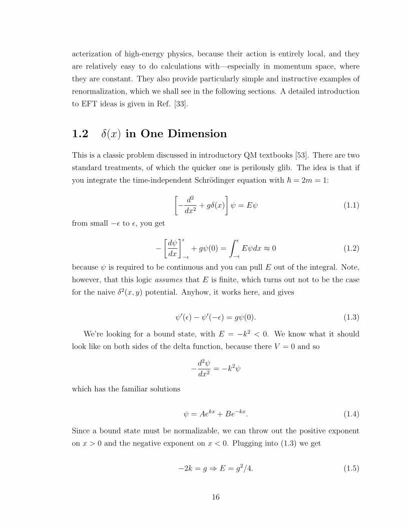
1.2 δ(x) in One Dimension
This is a classic problem discussed in introductory QM textbooks [53]. There are two
standard treatments, of which the quicker one is perilously glib. The idea is that if
you integrate the time-independent Schrodinger equation with ~ = 2m = 1:[− d2
dx2+ gδ(x)
]ψ = Eψ (1.1)
from small −ε to ε, you get
−[dψ
dx
]ε−ε
+ gψ(0) =
∫ ε
−εEψdx ≈ 0 (1.2)
because ψ is required to be continuous and you can pull E out of the integral. Note,
however, that this logic assumes that E is finite, which turns out not to be the case
for the naive δ2(x, y) potential. Anyhow, it works here, and gives
ψ′(ε)− ψ′(−ε) = gψ(0). (1.3)
We’re looking for a bound state, with E = −k2 < 0. We know what it should
look like on both sides of the delta function, because there V = 0 and so
−d2ψ
dx2= −k2ψ
which has the familiar solutions
ψ = Aekx +Be−kx. (1.4)
Since a bound state must be normalizable, we can throw out the positive exponent
on x > 0 and the negative exponent on x < 0. Plugging into (1.3) we get
−2k = g ⇒ E = g2/4. (1.5)
16
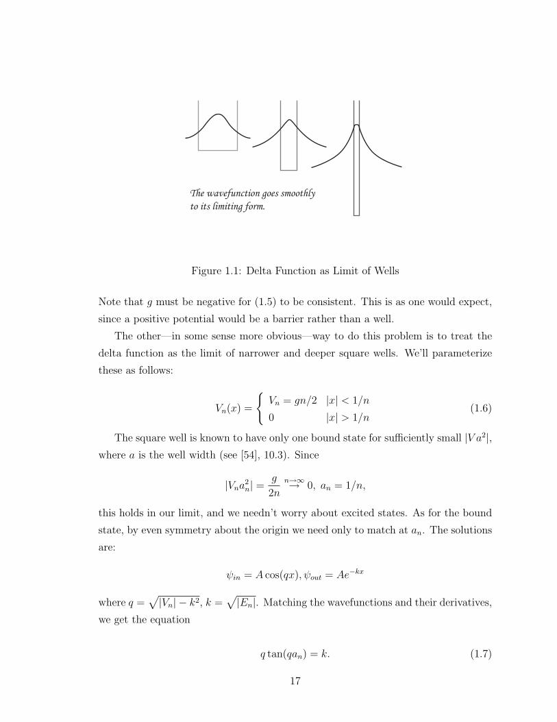
The wavefunction goes smoothlyto its limiting form.
Figure 1.1: Delta Function as Limit of Wells
Note that g must be negative for (1.5) to be consistent. This is as one would expect,
since a positive potential would be a barrier rather than a well.
The other—in some sense more obvious—way to do this problem is to treat the
delta function as the limit of narrower and deeper square wells. We’ll parameterize
these as follows:
Vn(x) =
Vn = gn/2 |x| < 1/n
0 |x| > 1/n(1.6)
The square well is known to have only one bound state for sufficiently small |V a2|,where a is the well width (see [54], 10.3). Since
|Vna2n| =
g
2n
n→∞→ 0, an = 1/n,
this holds in our limit, and we needn’t worry about excited states. As for the bound
state, by even symmetry about the origin we need only to match at an. The solutions
are:
ψin = A cos(qx), ψout = Ae−kx
where q =√|Vn| − k2, k =
√|En|. Matching the wavefunctions and their derivatives,
we get the equation
q tan(qan) = k. (1.7)
17
Since 0 ≤ k2 < |Vn|, qx ≤√|Vna2
n| → 0 and we can use the small angle approximation
q2an = k ⇒ g
2− k2
nan = kn (1.8)
where I’ve added subscripts to emphasize that the energy depends on n. Now this
can be rewritten as
g
2= kn(1 + knan)
and since knan ≤ qnan → 0, we get (1.5) again.
Scattering
We can apply a similar analysis to the scattering sector—that is, positive-energy
states—instead of the bound state sector. Recall that in one-dimensional scattering
our usual “observable” is the asymptotic phase shift we get if we send in the wave
e−ikx. It’s convenient for later purposes to send in a rather unconventional waveform
that’s symmetric about the origin: so that there’s a wave Aeikx coming in from the
left, and a wave Aeikx from the right. This makes the problem symmetric about
the origin, so that we can reduce it to a problem on a half-line. From our previous
analysis we know that the boundary condition at the origin is
g
2ψ(0) = ψ′(0+). (1.9)
The general form of the wavefunction (including the reflected wave) is Ae−ikx+Beikx
on the right half-line, and imposing the boundary condition on this we get
−i2kg
=A+B
A−B(1.10)
Now we can replace g by 2kb where kb is the bound state energy1, because of our
previous calculation. (In the case of the δ function it’s just a renaming, but one
could also think of it as a trivial example of renormalization, as the short-distance
coupling has been replaced by a long-distance observable in the theory.) Rearranging
this expression, we get
B
A=k − ikbk + ikb
(1.11)
1Strictly, Eb = k2b is the bound state energy, but since kb is much more useful, we will freely refer
to it as an energy.
18
B/A has magnitude one; the phase angle δ is what’s generally considered the most
useful scattering observable, since the asymptotic behavior of the wavefunction is
A(e−ikx + eiδeikx).
tan δ =−2kkbk2 − k2
b
. (1.12)
A feature of particular interest is the singularity in tan δ at k = kb; this is an instance
of a general result known as Levinson’s theorem [62], which we will discuss later (see
Chapter 7).
We could also have sent in a more conventional waveform e−ikx from the right, and
solved the problem without assuming symmetry. In this case we would have arrived
at the equation
ik
kb=A+B
B.
This can be rearranged as
B
A=
kbik − kb
,
and evidently the magnitude isn’t always one. The phase shift is a less complete
description for this problem, but it also has a simpler form:
tan δ =k
kb.
Now let’s add a dimension.
1.3 The 2D Schrodinger Equation
Separating variables in polar coordinates in the two-dimensional Schrodinger equation
[60] gives us the equations
d2Θ
dθ2+m2Θ = 0 (1.13)
and
1
r
d
dr
(rdR
dr
)+
(k2 − m2
r2− V
)= 0 (1.14)
19
where m is a constant introduced in the separation of variables, and must be an
integer in order to have Θ(θ) be single-valued. (1.14) can often be rewritten in the
sometimes more useful form
d2R
dr2+
1
r
dR
dr+
(k2 − m2
r2− V
)R = 0. (1.15)
In free space, this reduces to Bessel’s equation [56]
r2d2R
dr2+ r
dR
dr+ (k2r2 −m2)R = 0 (1.16)
to which the two solutions are the functions Jm(kr) and Nm(kr) (a.k.a. Ym), called
respectively the Bessel and Neumann functions of order m. (Note that a constant
potential would add on to k2r2 and thus change the argument of the Bessel functions
to qr, just as we do with trig functions.) In fact, Bessel functions bear several re-
semblances to sines and cosines, as we’ll have occasion to see. Bessel’s equation does
not require m to be an integer, and in fact there are even Bessel functions of complex
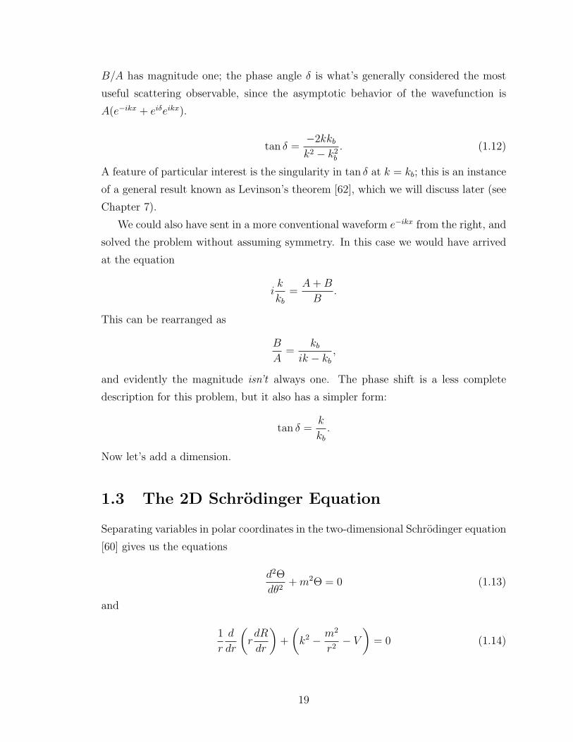
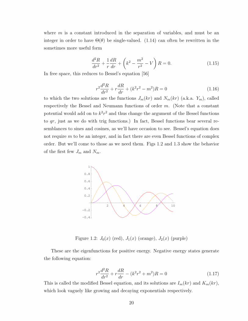
order. But we’ll come to those as we need them. Figs 1.2 and 1.3 show the behavior
of the first few Jm and Nm.
2 4 6 8 10
-0.4
-0.2
0.2
0.4
0.6
0.8
1
Untitled-1 1
Figure 1.2: J0(x) (red), J1(x) (orange), J2(x) (purple)
These are the eigenfunctions for positive energy. Negative energy states generate
the following equation:
r2d2R
dr2+ r
dR
dr− (k2r2 +m2)R = 0 (1.17)
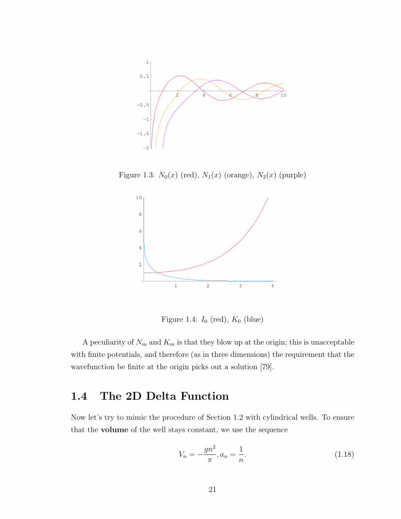
This is called the modified Bessel equation, and its solutions are Im(kr) and Km(kr),
which look vaguely like growing and decaying exponentials respectively.
20
2 4 6 8 10
-2
-1.5
-1
-0.5
0.5
1
Untitled-1 1
Figure 1.3: N0(x) (red), N1(x) (orange), N2(x) (purple)
1 2 3 4
2
4
6
8
10
Untitled-1 1
Figure 1.4: I0 (red), K0 (blue)
A peculiarity of Nm and Km is that they blow up at the origin; this is unacceptable
with finite potentials, and therefore (as in three dimensions) the requirement that the
wavefunction be finite at the origin picks out a solution [79].
1.4 The 2D Delta Function
Now let’s try to mimic the procedure of Section 1.2 with cylindrical wells. To ensure
that the volume of the well stays constant, we use the sequence
Vn = −gn2
π, an =
1
n. (1.18)
21
Note that there’s only one interior eigenvalue for any m, since the Neumann functions
are unacceptable at the origin for a potential without singularities. For the ground
state (m = 0) the solutions are
ψin = AJ0(qr), ψout = BK0(kr). (1.19)
Matching the wavefunctions and their derivatives at an gives us
qJ ′0(qa)
J0(qa)= k
K ′0(ka)
K0(ka), (1.20)
which we would like to simplify, but can’t, because
(qnan)2 → gn2 − k2
n2.
We have no justification, at this time, for assuming that the arguments are either
small or large, so we’re stuck. To see what’s going wrong here, let’s look at the
unseparated Schrodinger’s equation
−(∇2 + gδ2(r))ψ = −k2ψ. (1.21)
We are looking for a ground state, so we can restrict ourselves to m = 0, which
implies cylindrical symmetry. Since any solution must be a free-space solution except
at the origin, our eigenfunction must be of the form K0(kr) where −k2 is the bound
state energy. Suppose k < ∞. Then the rhs vanishes if you integrate the equation
over a small disc centered at the origin. The first term is ∇2(log r) near the origin.
Since log r is the Green’s function for Laplace’s equation in two dimensions [56] (it’s
parallel to 1/r in three dimensions), the volume integral returns a finite quantity
(the “enclosed charge”). However, K0 blows up at the origin and the second term is
infinite, so the lhs cannot add up to zero. Therefore there are no finite energy bound
states. However, since it’s the case that arbitrarily weak 2D square wells have bound
states, we would like the attractive delta function to have one. We can do this by
renormalizing the delta function.
1.5 Renormalizing the 2D Delta Function
Our theory diverges because the “real” short distance behavior isn’t accurately char-
acterized by our delta function. The first step is to regularize our theory by using
22
0.1 0.2 0.3 0.4cutoff
0.2
0.4
0.6
0.8
1
1.2
1.4
coupling
RG numerical.nb 1
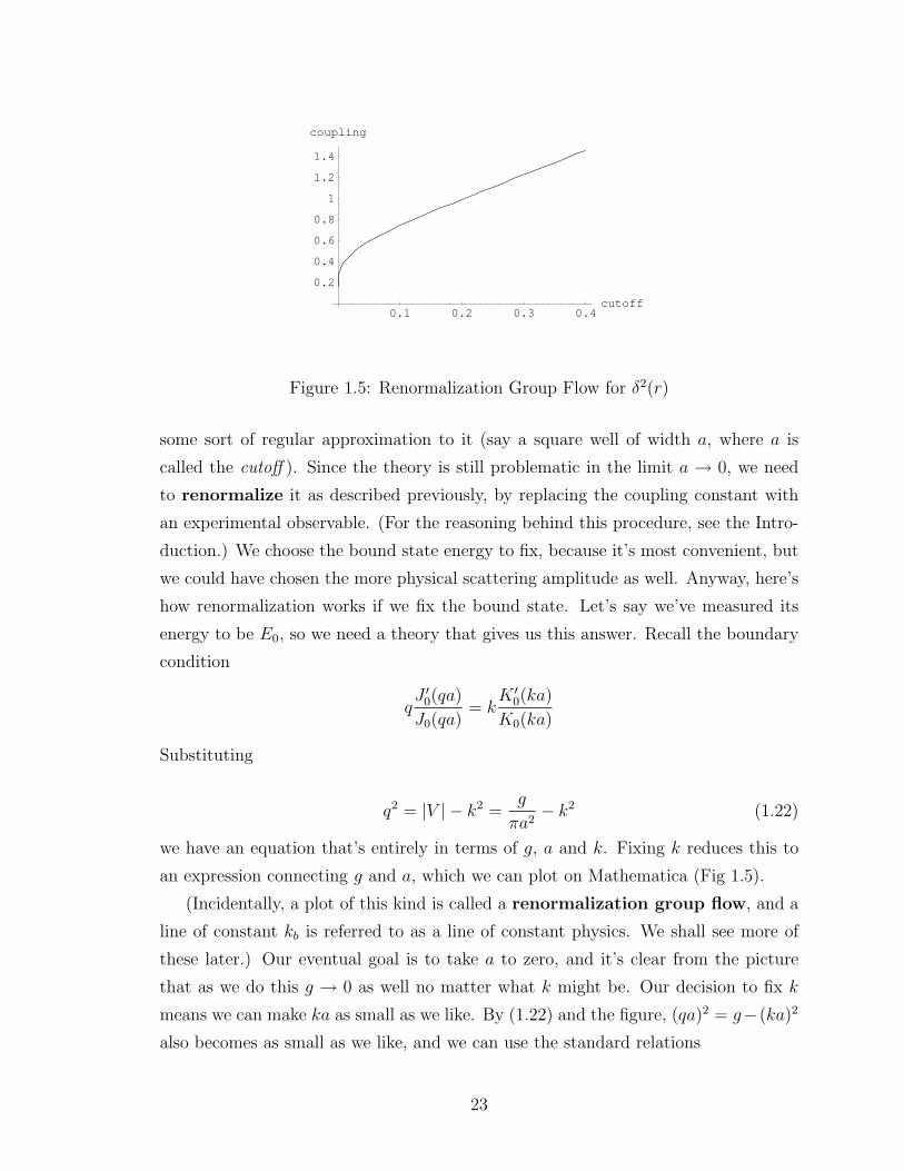
Figure 1.5: Renormalization Group Flow for δ2(r)
some sort of regular approximation to it (say a square well of width a, where a is
called the cutoff ). Since the theory is still problematic in the limit a → 0, we need
to renormalize it as described previously, by replacing the coupling constant with
an experimental observable. (For the reasoning behind this procedure, see the Intro-
duction.) We choose the bound state energy to fix, because it’s most convenient, but
we could have chosen the more physical scattering amplitude as well. Anyway, here’s
how renormalization works if we fix the bound state. Let’s say we’ve measured its
energy to be E0, so we need a theory that gives us this answer. Recall the boundary
condition
qJ ′0(qa)
J0(qa)= k
K ′0(ka)
K0(ka)
Substituting
q2 = |V | − k2 =g
πa2− k2 (1.22)
we have an equation that’s entirely in terms of g, a and k. Fixing k reduces this to
an expression connecting g and a, which we can plot on Mathematica (Fig 1.5).
(Incidentally, a plot of this kind is called a renormalization group flow, and a
line of constant kb is referred to as a line of constant physics. We shall see more of
these later.) Our eventual goal is to take a to zero, and it’s clear from the picture
that as we do this g → 0 as well no matter what k might be. Our decision to fix k
means we can make ka as small as we like. By (1.22) and the figure, (qa)2 = g−(ka)2
also becomes as small as we like, and we can use the standard relations
23
J ′0(x) = −J1(x), K′0(x) = −K1(x) (1.23)
and the small argument approximations
J0(x) ≈ 1, J1(x) ≈ x/2, K0(x) ≈ − log x,K1(x) ≈ 1/x (1.24)
to simplify the boundary condition to the form
q(−qa/2) = k−1/ka
− log(ka), (1.25)
which simplifies to
−q2a2 =2
log(ka). (1.26)
Using (1.22) and dropping the term that’s second order in a, we get
log(kbsa) = −2π/g, (1.27)
which can be rearranged to make E = k2 the subject:
Ebs =1
a2e−4π/g. (1.28)
Now we use this relation to calculate other quantities in terms of the BS energy. Let’s
consider the scattering problem. Lapidus [59] works out the m = 0 scattering phase
shift for a square well to be
tan(δ0) =kJ ′0(ka)J0(qa)− qJ ′0(qa)J0(ka)
kN ′0(ka)J0(qa)− qJ ′0(qa)N0(ka)
(1.29)
by the usual procedure of matching wavefunctions and their derivatives at the bound-
aries. Since k is fixed independently (by the incoming wave), for small a we can use
(1.22), leaving out the second order (in ka) terms, to get
qa =√g = −1/
√log(kbsa). (1.30)
Since our renormalization scheme has g → 0, we can use small-argument approxima-
tions for all the Bessel functions. The leading terms are:
J0(x) ≈ 1, J1(x) ≈ x/2, N0(x) ≈ (2/π) log x,N1(x) ≈ (2/πx)
Plugging in the expansions and dropping second-order terms, we get
24
tan δ0 =
πlog(kbsa)
2− 2 log(ka)log(kbsa)
(1.31)
which simplifies to
tan δ0 = − π
2 log(kbs/k). (1.32)
The important thing about this result is that our final answer is independent of
the value of a, so the a → 0 limit is simple. This is the hallmark of a correctly
renormalized theory.
Refs. [55] and [46] prove the renormalizability of the scattering problem using the
Born approximation and Fourier transform methods.
1.6 Scale Invariance and the Anomaly
An interesting thing about the Schrodinger equation with ~ = 2m = 1 is that all
dimensions can be expressed in terms of lengths. One can see from the form of the
equation
−∇2ψ + V ψ = Eψ
that (if the energy terms are to be dimensionally consistent with the first term) energy
must have dimensions [length]−2. Mass has no dimensions, by construction, and the
dimensions of time can be seen from the uncertainty relation
∆E∆t =1
2
to be [length]2. With most normal potentials, one can use dimensional analysis [47]
to predict the bound state energy (to within a multiplicative constant) from the scales
intrinsic to the problem. Two examples:
• The Harmonic Oscillator. The scale is set by the constant in ax2, which has
dimensions [length]−4. So if we want to construct a bound state energy it must
be of the form√a up to a multiplicative constant. a is normally written as ω2,
which gives E = ω, as we expect.
• The Infinite Well. The only intrinsic parameter is the width L. To construct
an energy out of this we clearly need L−2.
25

It should be noted that this reasoning sometimes breaks down. A good example is
the case of singular potentials 1/rn, n > 2, where the bound state energies depend on
scales set by the short-distance physics, rather than the intrinsic scales of our effective
theory.
A particularly interesting situation arises with the δ2 and 1/r2 potentials, since the
coupling constant is dimensionless and so there is no intrinsic scale to the problems.
The Hamiltonians are scale invariant, i.e. they are invariant under a dilation r → λr.
This is obvious in the case of the inverse square potential in 1D:
Hx = − d2
dx2+
g
x2, Hλx = − d2
d(λx)2+
g
(λx)2=
1
λ2Hx (1.33)
Since Hλxψ(λx) has the same eigenvalues as Hxψ(x) (it’s just a relabeling of vari-
ables), it follows from our result that
Hxψ(x) = Eψ(x) ⇒ Hxψ(λx) = λ2Eψ(λx) (1.34)
Therefore, if E is an eigenvalue then so is λ2E, and if there are any (finite energy)
bound states then all negative energy states are bound states. This is impossible
because it violates the requirement that eigenfunctions be orthogonal2 (which is re-
lated to self-adjointness), so a scale invariant QM potential can have no bound states
except at −∞. The proof for δ2(x) is similar, but depends on the well-known fact
that
δn(ax) =1
anδn(x)
(to compensate for the Jacobian).
This is what happens with the naive δ2(x) potential. What renormalization does
is to introduce a scale—the renormalized bound state energy—into this problem by
hand, thus breaking the scale invariance of the classical potential. This phenomenon
is known as the anomaly in quantum mechanics, and is an example of a common
occurrence in field theory known as dimensional transmutation, which is said to
occur when a dimensionless quantity (the coupling) is traded in for a quantity with
dimensions (the bound state energy).
2Intuitively, the eigenvectors corresponding to infinitesimally separated eigenvalues should look
exactly alike, in which case they certainly can’t be orthogonal.
26
1.7 The 2D Delta Function as Limit of Rings
This is the method used by [55]. The “regular” approximate potential is a ring of 1D
delta functions of radius ε:
V =gδ(r − ε)
2πε(1.35)
(The denominator is clearly needed to have g be dimensionless, and it’s also in-
tuitive that the 1-D delta functions must get stronger as their “density” decreases.)
We’re looking for a bound state with m = 0, which implies spherical symmetry. We
can move to momentum space, where the ∇’s turn to p’s, and our equation has the
following form:
−p2φ(p) + gψ(ε) = k2φ(p) (1.36)
We can solve this for φ(p):
φ(p) = gψ(ε)
(1
p2 + k2
)(1.37)
We can transform this back into position space. The inverse Fourier transform of the
quantity in parentheses is known (see [56]) to be K0(kr)/2π, so we get
ψ(r) = gψ(ε)K0(kr)/2π (1.38)
Plugging in r = ε and cancelling out the ψ’s3, we get the condition
2π = gK0(kε) (1.39)
Since K0 is logarithmic at the origin, we can rearrange this expression as
k =1
εe−2π/g
which is of the same form as (1.27). The rest of the renormalization proceeds just as
it did with the square well, and we won’t go into the details.
3This requires ψ(ε) 6= 0, but otherwise our wavefunction would be trivial.
27
1.8 The 3D Delta Function
Again, we might want to solve this potential as a limit of spherical wells, of the form
V = − g43πa3
(1.40)
The radial Schrodinger equation with l = 0 looks exactly like its 1D counterpart in
terms of u = ψ/r. The difference is that in order to ensure that ψ stays regular at
the origin we require u(0) = 0. This means that the ground state is a sine and not
a cosine—and that for sufficiently weak coupling there is no ground state. Matching
equations and derivatives at the boundaries, we get
q cot qa = k ⇒√
g
a3− k = k tan
(√g
a3− ka
)(1.41)
There are three possibilities. One is that q → 0 slower than a, in which case the
argument of tan qa gets very big, and we know that x intersects tanx infinitely often,
so the equations don’t flow anywhere in particular. The second is that g → 0 fast
enough, so that we’re in the small argument regime. In this case, we can expand
cot qa ≈ 1/qa, so q cot qa→ 1/a, and we can’t renormalize because the coupling has
disappeared from the equations. The third possibility is that g falls off at exactly
the same rate as a, but this is not a helpful regime for analytic work. In fact this
approach is problematic for several reasons, one of which is that the regular solutions
all obey ψ(0) = 0 and the “real” solution doesn’t. It turns out that one can regularize
the problem with a square well, but needs to parameterize the wells in a non-obvious
way to have the limit work out [64]. The easiest solution is by means of self-adjoint
extensions (see Chapter 2); however, delta function shells also do the trick. If we solve
the equation by Fourier transformation as before, and recall that the appropriate 3D
Green’s function is e−kr/r, our consistency criterion becomes
1 = −ge−kba
2πa. (1.42)
We can use this to solve the scattering problem in the usual way, remembering that
the derivative jumps at the delta function:
C sin(ka) = Aeika +Be−ika (1.43)
kC cos(ka) +gC sin(ka)
2πa2= ik(Aeika −Be−ika). (1.44)
28
And so
k cot(ka) +g
2πa2= ik
[Aeika −Be−ika
Aeika +Be−ika
]. (1.45)
The rhs simplifies considerably if we drop all higher-order terms. Substituting for γ
from (1.39) we get
cot(ka)− 1
kae−kba= i
[A−B
A+B
](1.46)
Expanding the lhs and keeping terms of up to zeroth order in a, we get the singular
terms to cancel out and leave us with
ikbk
=
[A−B
A+B
](1.47)
from which we can derive an expression for the phase shift that is consistent with
self-adjoint extensions (Chapter 2).
1.9 More Dimensions, etc.
Since most of this thesis takes place in three or fewer dimensions, the properties of
higher-dimensional delta functions are not that relevant. In five or more dimensions all
cutoff regularizations give a trivial result, though the popular (in QFT) technique of
dimensional regularization sometimes allows bound states. (See [68] for more details.)
Which of these regulation schemes do we trust, and to what extent are these effects
scheme-independent? We will look at these issues again in later chapters, in the richer
context of power-law potentials.
1.10 The δ′(x) Potential
The delta function and its derivatives are less unfamiliar in momentum space than in
position space. We know that the Fourier transform of δ(x) is∫δ(x)ψ(x)e−ipxdx = ψ(0),
a constant. Now δ′(x) is a little more interesting.∫δ′(x)ψ(x)e−ipxdx = −
∫δ(x)[ψ′(x)− ipψ(x)]e−ipxdx = ipψ(0)− ψ′(0),
29

so δ′(x) is basically dual to the entirely mundane operation of multiplication by p in
momentum space. That a function appears in a certain context in quantum mechanics
does not make it useful as a potential, but it sometimes appears as a short-distance
“counterterm” in renormalization. (We’ll see what this means in Ch. 5.)
The 1D delta function derivative is particularly nice because, along with the 2D
delta function, it possesses the mysterious property of scale invariance. (δ′(x) has
dimensions of length−2.) If you integrate the Schrodinger equation around zero,
− dψ
dx
∣∣∣∣ε−ε
+ g
∫ ε
−εδ′(x)ψ(x) = k2
∫ ε
−εψ(x)
the potential term can be integrated by parts to give
−g∫ ε
−εδ(x)ψ′(x) = −gψ′(0)
For this to be meaningful the derivative must be continuous at zero, so we can throw
out the derivative terms. But if we do so the result is bound to be trivial for finite
energies, since ψ is regular and its integral vanishes. However, a bound state with
infinite energy is still a possibility. Its integral in a region right around the origins
would go roughly as ψ(0)a for tiny a. (It turns out that integrating from −ε to ε
doesn’t work, because the function we’re looking for is odd.)
It might seem silly to force this problem to have a bound state. However, we do
have a bound state in mind, and it’s an odd version of the delta function’s bound
state:
ψ = sgn(x)e−k|x|
Our desire for a bound state is motivated partly by Simon’s theorem (see Chapter 3),
which states that there should be one for any short-range not-too-pathological odd
potential.
The situation is symmetric to the delta function; there we had a discontinuity
in the derivative proportional to ψ(0); here we have a discontinuity in the function
proportional to ψ′(0), but the derivative is continuous. The fact that the wavefunction
is discontinuous is enough to irritate most people with the δ′(x) potential, and maybe
its physical applications are limited. However, if you think of wavefunctions as waves
on a string, it is possible to make sense of this potential. First, notice that the delta
function is a cusp, of the sort that would correspond to having a bead at the origin
(or a spring pulling down). The “mass” is proportional to the derivative at the origin,
30
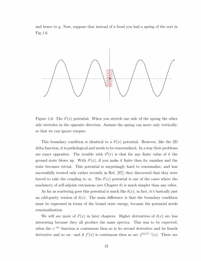
and hence to g. Now, suppose that instead of a bead you had a spring of the sort in
Fig 1.6.
Figure 1.6: The δ′(x) potential. When you stretch one side of the spring the other
side stretches in the opposite direction. Assume the spring can move only vertically,
so that we can ignore torques.
This boundary condition is identical to a δ′(x) potential. However, like the 2D
delta function, it is pathological and needs to be renormalized. In a way their problems
are exact opposites. The trouble with δ2(r) is that for any finite value of k the
ground state blows up. With δ′(x), if you make k finite then ka vanishes and the
state becomes trivial. This potential is surprisingly hard to renormalize, and was
successfully treated only rather recently in Ref. [97]; they discovered that they were
forced to take the coupling to ∞. The δ′(x) potential is one of the cases where the
machinery of self-adjoint extensions (see Chapter 8) is much simpler than any other.
As far as scattering goes this potential is much like δ(x); in fact, it’s basically just
an odd-parity version of δ(x). The main difference is that the boundary condition
must be expressed in terms of the bound state energy, because the potential needs
renormalization.
We will see more of δ′(x) in later chapters. Higher derivatives of δ(x) are less
interesting because they all produce the same spectra. This was to be expected;
when the e−kx function is continuous then so is its second derivative and its fourth
derivative and so on—and if f ′(x) is continuous then so are f (3,5,7...)(x). There are
31

two distinct δ function like interactions in one dimension; even this is anomalously
rich, as in two or three dimensions all point interactions are delta functions, and in
d ≥ 4 there are no point interactions at all [68].
32
Chapter 2
Self-Adjoint Extensions
The first three sections are meant to be a hurried and heuristic introduction to some
ideas from functional analysis. Formal proofs have been avoided wherever possible;
they can be found in Refs. [71], VIII-X; [69], 11-14; and [75], X.
2.1 Hilbert Space
Operators are “functions” that act on functions, which is to say, they take functions
to other functions. So, if we’re talking about functions of a single real variable x,
f → f 2 is an operator, and so is f → dfdx
. Now, we want to distinguish operators that
behave sensibly from operators that don’t; and part of this is determining whether
they act similarly on similar functions, e.g. we’d worry about an operator that sent
x2 to x4 and x2 + εx3 (arbitrarily small ε) to zero. A useful approach is to treat
functions as “points” in an abstract space, and to introduce a concept of distance
between two functions. This is the basic idea behind Hilbert spaces.
Of course, we aren’t interested in all functions but only in those that are relatively
well-behaved. As a first guess we might want to restrict our attention to continuous
functions. However, many of the properties of our space depend on its “completeness”
(the existence of limits, in the space, to convergent sequences in the space) and it’s
easy to create sequences of continuous functions that have discontinuous limits, so
that won’t quite do.
It turns out that achieving completeness is pretty difficult. The details are highly
technical and irrelevant to our purposes, so we’ll just state the definitions and request
the reader not to look at them too closely.
33
0.2 0.4 0.6 0.8 1
0.2
0.4
0.6
0.8
1
Untitled-2 1
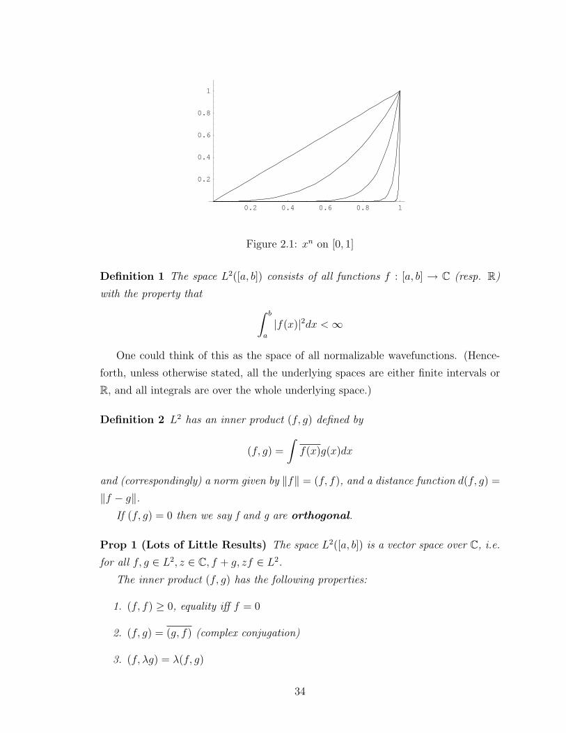
Figure 2.1: xn on [0, 1]
Definition 1 The space L2([a, b]) consists of all functions f : [a, b] → C (resp. R)
with the property that ∫ b
a
|f(x)|2dx <∞
One could think of this as the space of all normalizable wavefunctions. (Hence-
forth, unless otherwise stated, all the underlying spaces are either finite intervals or
R, and all integrals are over the whole underlying space.)
Definition 2 L2 has an inner product (f, g) defined by
(f, g) =
∫f(x)g(x)dx
and (correspondingly) a norm given by ‖f‖ = (f, f), and a distance function d(f, g) =
‖f − g‖.If (f, g) = 0 then we say f and g are orthogonal.
Prop 1 (Lots of Little Results) The space L2([a, b]) is a vector space over C, i.e.
for all f, g ∈ L2, z ∈ C, f + g, zf ∈ L2.
The inner product (f, g) has the following properties:
1. (f, f) ≥ 0, equality iff f = 0
2. (f, g) = (g, f) (complex conjugation)
3. (f, λg) = λ(f, g)
34
4. (f, g + h) = (f, g) + (f, h)
The norm has the following properties:
1. ‖f‖ ≥ 0, equality iff f = 0
2. |(f, g)| ≤ ‖f‖‖g‖ (Cauchy-Schwarz inequality)
3. ‖f + g‖ ≤ ‖f‖+ ‖g‖ (the triangle inequality)
There are some subtleties about f = g. Because point discontinuities don’t affect
the integral, two functions that differ at isolated points are considered the same (i.e.
we think of them as the same point in our function space). There’s a more general
form of this equivalence, called “equality almost everywhere,” but that need not
concern us.
The upshot is that for many (though not all) purposes, L2 behaves like Rn, if you
think of the inner product as a dot product.
An important difference between L2 and physical space is that L2 is infinite-
dimensional, i.e. you can’t write all functions as a finite sum of basis functions.
This is clear enough, since there are so many different types of functions. It is a
remarkable property of L2([a, b]) that it does have a countably infinite basis, because
every function in it can be written as the sum of its Fourier series. As is usual with
infinite series, there are issues involving convergence. Our definition of convergence
is as follows:
Definition 3 We say fk → f if ‖f − fk‖ gets arbitrarily small for large k, i.e. if∫|f − fk|2 → 0
This definition is quite different from pointwise convergence, which implies that the
function converges to its limit at every point. (i.e. |f(x)−fk(x)| gets arbitrarily small
for each x with sufficiently large k). It’s possible for either form of convergence to
hold without the other, as shown by the two examples below. (The first is a standard
example in analysis textbooks; the second is a variant of a standard example.)
Example 1
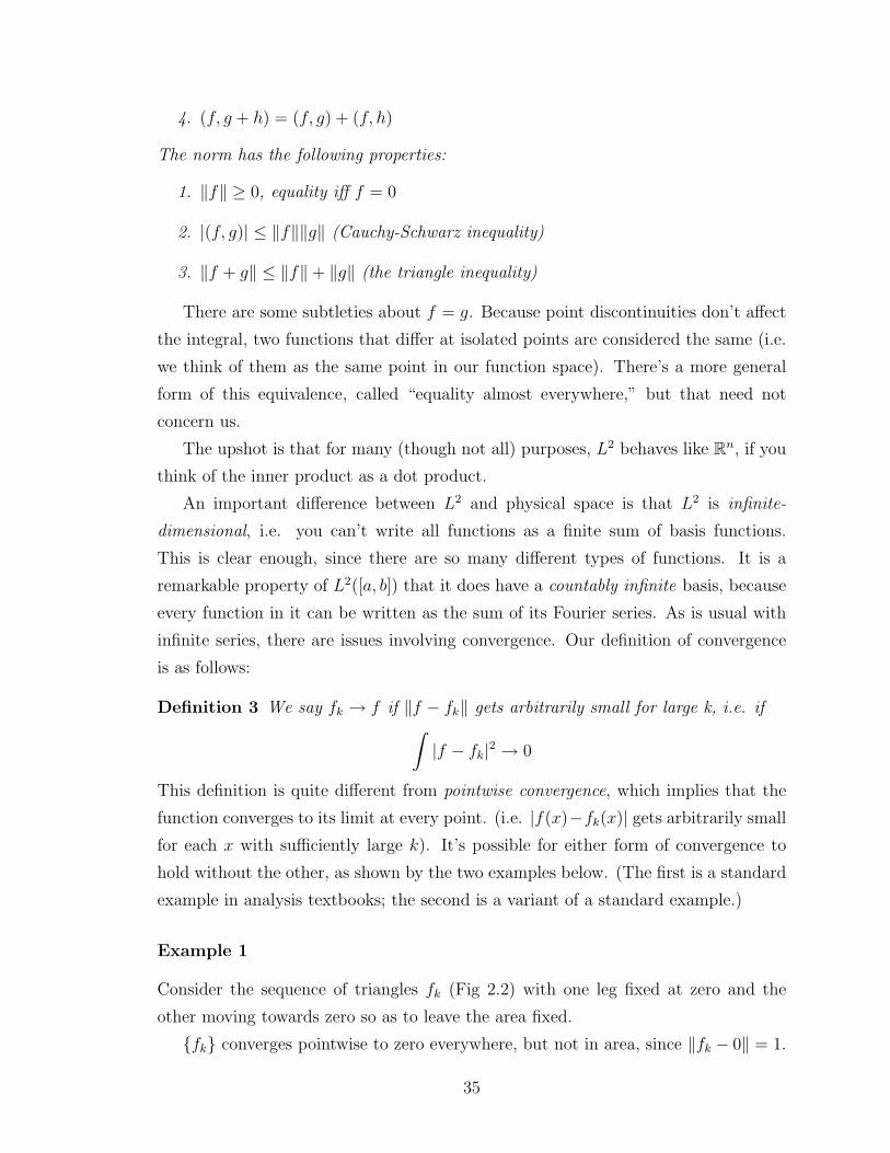
Consider the sequence of triangles fk (Fig 2.2) with one leg fixed at zero and the
other moving towards zero so as to leave the area fixed.
fk converges pointwise to zero everywhere, but not in area, since ‖fk − 0‖ = 1.
35
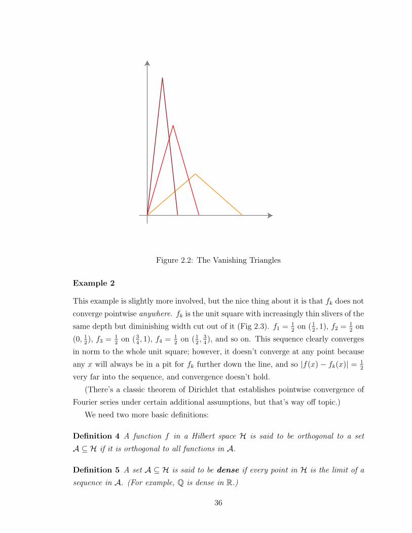
Figure 2.2: The Vanishing Triangles
Example 2
This example is slightly more involved, but the nice thing about it is that fk does not
converge pointwise anywhere. fk is the unit square with increasingly thin slivers of the
same depth but diminishing width cut out of it (Fig 2.3). f1 = 12
on (12, 1), f2 = 1
2on
(0, 12), f3 = 1
2on (3
4, 1), f4 = 1
2on (1
2, 3
4), and so on. This sequence clearly converges
in norm to the whole unit square; however, it doesn’t converge at any point because
any x will always be in a pit for fk further down the line, and so |f(x)− fk(x)| = 12
very far into the sequence, and convergence doesn’t hold.
(There’s a classic theorem of Dirichlet that establishes pointwise convergence of
Fourier series under certain additional assumptions, but that’s way off topic.)
We need two more basic definitions:
Definition 4 A function f in a Hilbert space H is said to be orthogonal to a set
A ⊆ H if it is orthogonal to all functions in A.
Definition 5 A set A ⊆ H is said to be dense if every point in H is the limit of a
sequence in A. (For example, Q is dense in R.)
36

f_1 f_2
f_100 f_200
Figure 2.3: The Disappearing Gash
(So, for instance, the space consisting of all functions
f(x) =k∑
n=1
aneinx (2.1)
is dense in L2([−π, π]) by virtue of the convergence of Fourier series.)
The following proposition will be useful later.
Prop 2 If A is dense in H and f is orthogonal to A, then f = 0.
Proof. Suppose f⊥A, f 6= 0. Pick a sequence fk ∈ A that converges to f .
(f, f) = (f, f)− (f, fk) = (f, f − fk)
since (f, fk) = 0 by hypothesis. Now we can use the Cauchy-Schwarz inequality:
‖f‖2 = |(f, f)| = |(f, f − fk)| ≤ ‖f‖‖f − fk‖
and since f 6= 0 we get
37
‖f‖ ≤ ‖f − fk‖
which is impossible because f 6= 0 but f − fk gets arbitrarily small.
And we’ll close this section with a major result in real analysis that will be useful
to us:
Theorem 1 (Stone-Weierstrass Approximation Theorem) C∞0 (I), the set of
all bounded, infinitely differentiable functions on I, is dense in L2(I), where I ⊆ R is
a finite or infinite interval.
This means that every function can be approximated arbitrarily well by a very
well-behaved function. For finite intervals, this result follows since all finite Fourier
series sums are members of C∞0 . In practice we normally need just C2[⊇ C∞
0 ] with
maybe a few pointwise conditions (say, “everything and its derivative must vanish at
the origin”) and the issue of density is rarely relevant. We generally assume that all
sets we are working with are dense.
2.2 Linear Operators and their Domains
A linear operator L : D ⊆ H → H acts linearly on the function space, so L(af+bg) =
aLf+bLg (and L(0) = 0). dn
dxn is a linear operator, as is multiplication by a constant or
a function in the space. For many purposes linear operators are just infinite matrices,
and the familiar equation
Hψ = Eψ
is called an eigenvalue equation because of that analogy. However, the analogy some-
times breaks down, and a good example of how this happens is the issue of domains.
For example, the function f(x) = x−0.1 is a respectable member of L2([0, 1]), but its
derivative is not. What can be said about domains generally is stated in the following
proposition:
Prop 3 The domain of an operator A will be denoted as D(A).
1. D(λA) = D(A), λ ∈ C
38

2. D(A+B) = D(A) ∩D(B)
3. D(AB) = D(A) ∩R(B), where R(B) is the range of B
Definition 6 An operator A is said to be bounded if there’s a number λ such that
‖Af‖ ≤ λ‖f‖ for all functions in D(A).
The importance of operator domains is suggested by the following theorem:
Theorem 2 (Hellinger-Toeplitz) A Hermitian operator defined everywhere is bounded.
As luck would have it, Schrodinger operators are virtually never bounded.
Hermitian Operators and Adjoints
A Hermitian operator H has the property that, for all f, g ∈ D(H), (f,Hg) =
(Hf, g). Hermitian operators always have real eigenvalues and orthogonal eigen-
functions. However, the following commonly assumed properties are not generally
true of Hermitian operators:
1. They always generate unitary time evolution.
2. They always have well-defined adjoints.
3. Their adjoints are Hermitian.
4. They always have a complete set of eigenfunctions.
The rest of this section will be dedicated to discussing these points. First, the issue
of adjoints. The action of an adjoint H† is defined by (Hf, g) = (f,H†g), so of course
D(H†) ⊇ D(H), but the adjoint might be well-defined outside of D(H). Here’s a
simple example involving the 1-D infinite well (taken from Ref. [77]):
The Frailty of Hermeticity
This example, from [77], illustrates what can happen if we don’t think about operator
domains. The Hamiltonian for this system is
H = − ~2m
d2
dx2, |x| < L/2
Now consider the (not normalized) wavefunction
39
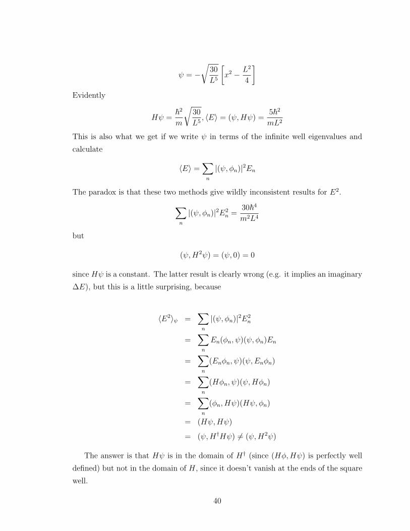
ψ = −√
30
L5
[x2 − L2
4
]Evidently
Hψ =~2
m
√30
L5, 〈E〉 = (ψ,Hψ) =
5~2
mL2
This is also what we get if we write ψ in terms of the infinite well eigenvalues and
calculate
〈E〉 =∑n
|(ψ, φn)|2En
The paradox is that these two methods give wildly inconsistent results for E2.∑n
|(ψ, φn)|2E2n =
30~4
m2L4
but
(ψ,H2ψ) = (ψ, 0) = 0
since Hψ is a constant. The latter result is clearly wrong (e.g. it implies an imaginary
∆E), but this is a little surprising, because
〈E2〉ψ =∑n
|(ψ, φn)|2E2n
=∑n
En(φn, ψ)(ψ, φn)En
=∑n
(Enφn, ψ)(ψ,Enφn)
=∑n
(Hφn, ψ)(ψ,Hφn)
=∑n
(φn, Hψ)(Hψ, φn)
= (Hψ,Hψ)
= (ψ,H†Hψ) 6= (ψ,H2ψ)
The answer is that Hψ is in the domain of H† (since (Hφ,Hψ) is perfectly well
defined) but not in the domain of H, since it doesn’t vanish at the ends of the square
well.
40

The domain of the adjoint is every φ such that (Hψ, φ) makes sense for
all ψ ∈ D(H).
All of this assumes that the action of H† is uniquely defined. Let’s see if that
works. Suppose we have an operator A, with two adjoints B1 and B2. Given x ∈D(A), y ∈ D(B1) ∩D(B2), it follows that
(x, (B1 −B2)y) = (x,B1y)− (x,B2y) = (Ax, y)− (Ax, y) = 0.
This implies that (B1 − B2)y⊥D(A). In general it’s impossible to improve on this,
but if D(A) is dense, it follows from prop 1.1.2 that (B1−B2)y = 0, and since this is
true for all y we have uniqueness of the adjoint.
For the rest of this chapter we assume that all our operators are densely
defined.
Definition 7 A self-adjoint operator is a Hermitian operator that has the same do-
main as its adjoint. (Equivalently: a Hermitian operator with a Hermitian adjoint.)
It turns out that only self-adjoint operators generate unitary time evolution; there-
fore it’s important for our Hamiltonians to be self-adjoint. Since D(H) ⊆ D(H†)
generally, one must extend a non-self-adjoint operator to make it self-adjoint. From
the definition of D(H†), as D(H) grows each f ∈ D(H†) needs to have well-defined
inner products with more vectors—it needs to make more sense, so to speak—so ex-
tending the operator domain involves constraining the adjoint domain... and, indeed,
failures of self-adjointness manifest themselves in physics mostly through ill-defined
boundary conditions.
Our next goal is to see how to construct self-adjoint extensions of a Hamiltonian.
2.3 Self-Adjoint Extensions
I recognize that this section is unpleasantly technical, but the central result sounds
pretty mysterious without justification. The idea is that H†, being potentially non-
Hermitian, might have complex eigenvalues, and you can restrict it to a Hermitian
operator by allowing only some combinations of the corresponding eigenvectors in the
domain. (The freedom you have in choosing this is normally indicative of additional
physics, which must be imposed by means of a boundary condition.) The key objects
in this process are
41
Definition 8 The positive (resp. negative) deficiency subspace, N±, of H is
the eigenspace of H† corresponding to eigenvalues ±i. The deficiency indices n±
are the dimensions of N±.
It turns out that any χ ∈ D(H†) can be written uniquely as follows:
χ = aφ+ bΨ+ + cΨ− (2.2)
where
φ ∈ D(H),Ψ± ∈ N±
In other words, D(H), N+, and N− are linearly independent. Be warned, however,
that the three spaces are not mutually orthogonal, since nothing is orthogonal to
D(H). If n+ = n−, we can define an “extension” Hθ to have the same action as
H† and be defined on D(Hθ) = φ + A(Ψ+ − UθΨ+) : φ ∈ D(H),Ψ+ ∈ N+,where Ψ± are vectors, A is a matrix, Uθ : N+ → N− is a unitary (strictly speaking,
“norm-preserving”) operator that characterizes the particular extension chosen. By
definition of N±,
Hθχ = Hφ+ i
n+∑k=1
λk(Ψ+,k + Uθ,kjΨ+,j) (2.3)
for all χ ∈ D(Hθ). For deficiency indices (1, 1), this is a subspace of D(H†) with b/c
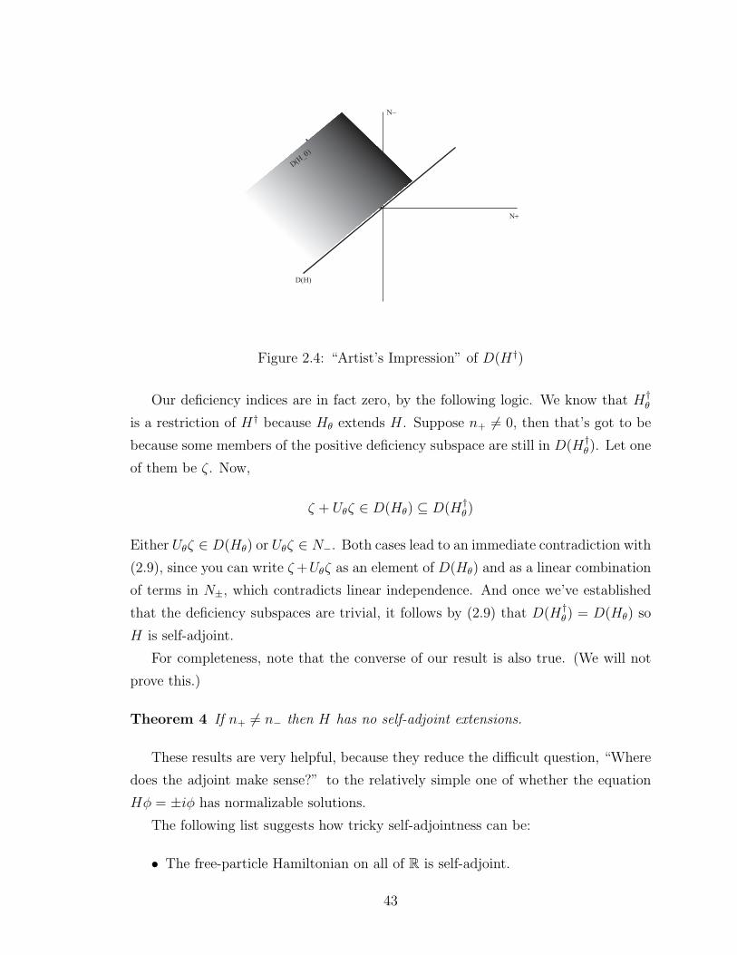
fixed at a phase angle. A schematic and unfaithful representation of what’s going on
is given in the figure below.1
(We will typically use the characterization:
D(Hθ) = φ+B(Ψ+ + VθΨ−) (2.4)
(Vθ unitary) which is equivalent because all vectors in N− are equivalent to Ψ− under
a unitary transformation.)
It’s straightforward to show that Hθ is symmetric. The importance of these ex-
tensions is that they are self-adjoint because of the following theorem:
Theorem 3 If n+ = n− = 0, H is self-adjoint or has a unique self-adjoint extension.
1Among other things that are wrong with the picture, the subspaces are not supposed to be
orthogonal, the angle is supposed to be a phase between vectors of equal magnitude, and D(H) is
infinite dimensional.
42
θ
Ν+
Ν−
D(H)
D(H_θ)
Figure 2.4: “Artist’s Impression” of D(H†)
Our deficiency indices are in fact zero, by the following logic. We know that H†θ
is a restriction of H† because Hθ extends H. Suppose n+ 6= 0, then that’s got to be
because some members of the positive deficiency subspace are still in D(H†θ). Let one
of them be ζ. Now,
ζ + Uθζ ∈ D(Hθ) ⊆ D(H†θ)
Either Uθζ ∈ D(Hθ) or Uθζ ∈ N−. Both cases lead to an immediate contradiction with
(2.9), since you can write ζ+Uθζ as an element of D(Hθ) and as a linear combination
of terms in N±, which contradicts linear independence. And once we’ve established
that the deficiency subspaces are trivial, it follows by (2.9) that D(H†θ) = D(Hθ) so
H is self-adjoint.
For completeness, note that the converse of our result is also true. (We will not
prove this.)
Theorem 4 If n+ 6= n− then H has no self-adjoint extensions.
These results are very helpful, because they reduce the difficult question, “Where
does the adjoint make sense?” to the relatively simple one of whether the equation
Hφ = ±iφ has normalizable solutions.
The following list suggests how tricky self-adjointness can be:
• The free-particle Hamiltonian on all of R is self-adjoint.
43
• The free Hamiltonian on [−L,L] has deficiency indices (2,2). One of its self-
adjoint extensions corresponds to the particle in a box.
• The Hamiltonian with Coulomb potential in three dimensions is self-adjoint,
but the radial equation is not.
• The Hamiltonian with a/r2 potential is self-adjoint for a > 3/4 but has defi-
ciency indices (1,1) below that.
• Hamiltonians with −xn potentials in one dimension (bottomless hills) are self-
adjoint for 0 < n ≤ 2 but need extensions for n > 2.
• The momentum operator on R+ has deficiency indices (0,1) and can’t be made
self-adjoint.
Generally, Hamiltonians of the usual form −∇2 + V , where V is reasonably well-
behaved, do have self-adjoint extensions. This is a consequence of the following
theorem:
Theorem 5 If H commutes with complex conjugation, i.e. if Hψ ≡ Hψ then H has
equal deficiency indices.
(For a proof, see [75].) Note that p does not commute with complex conjugation,
but is often self-adjoint in any case.
2.4 The Physics of Self-Adjoint Extensions
There is generally some physical reason behind the failure of self-adjointness, most
commonly an unspecified boundary condition. Our strategy will be as follows:
1. Find as small a domain as possible for the operator. How small we can make
this is limited by the requirement that H be dense. However, we can normally
restrict our original domain to C20 with the pointwise constraints that all func-
tions and their derivatives should vanish at boundaries, singularities, and other
dubious points.
2. This leaves the adjoint domain as essentially L2, so we don’t need to worry
about whether a particular normalizable solution is in the adjoint domain.
44

3. Calculate the deficiency indices and determine the corresponding eigenspaces.
4. Use Ψ± to determine the boundary conditions.
For all the examples below, we’ve assumed that the original operator is Hermi-
tian, the domain of definition is C2 vanishing at the boundaries (except as otherwise
specified), and that the adjoint domain is sufficiently large. The examples considered
below are all standard in the literature. A detailed treatment of how one finds the
adjoint domain is given in Chapter 8 for the one-dimensional free particle.
First, we consider a case where the operator is essentially self-adjoint, i.e.
where its deficiency indices are (0,0) but it still needs extension.
Momentum for Free Particle on the Real Line
Let our original domain be C∞0 , which we know to be dense, and the operator be i d
dx,
which we know to be Hermitian. Solving for deficiency indices
idψ
dx= ±iψ
we get Ψ± = e±x. Neither of these is normalizable; therefore there are no eigenfunc-
tions for ±i in L2 and our deficiency indices are (0,0). However, the adjoint domain
is considerably larger than the original domain and includes just about anything in
L2, since the result ∫ψdφ
dxdx = −
∫dψ
dxφdx
certainly does not require ψ ∈ H† to be infinitely differentiable. There’s no new
physics involved in finding a self-adjoint domain, however, so the distinction is not
important to physicists. For our purposes an essentially self-adjoint operator is self-
adjoint.
Free Particle on x > 0
This problem is underspecified; to see why, consider the corresponding problem with
waves on a string. Since we want to conserve amplitudes on our domain, the wave
must be reflected at the origin, but the reflector could be either fixed (a clamped end)
or movable (a ring sliding on a rod). The reflection coefficient is one both ways, but
the phase shifts are different, so the physics is not completely specified unless you
know the exact boundary condition.
45
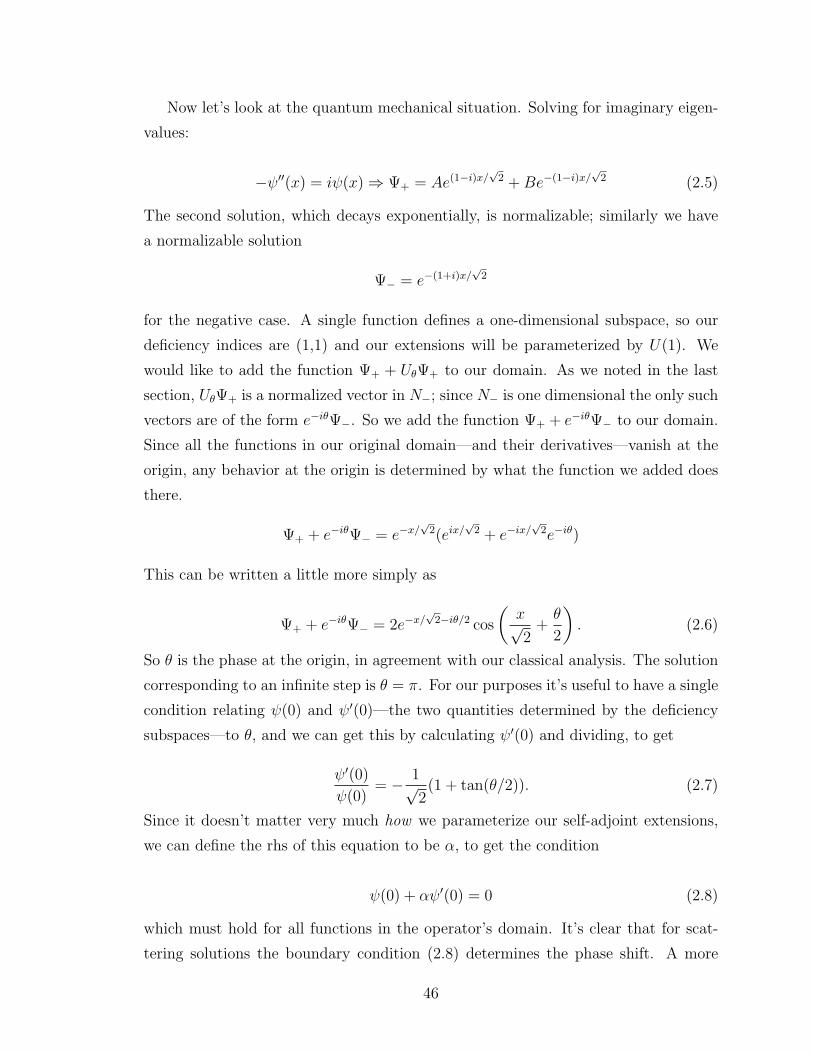
Now let’s look at the quantum mechanical situation. Solving for imaginary eigen-
values:
−ψ′′(x) = iψ(x) ⇒ Ψ+ = Ae(1−i)x/√
2 +Be−(1−i)x/√
2 (2.5)
The second solution, which decays exponentially, is normalizable; similarly we have
a normalizable solution
Ψ− = e−(1+i)x/√
2
for the negative case. A single function defines a one-dimensional subspace, so our
deficiency indices are (1,1) and our extensions will be parameterized by U(1). We
would like to add the function Ψ+ + UθΨ+ to our domain. As we noted in the last
section, UθΨ+ is a normalized vector in N−; since N− is one dimensional the only such
vectors are of the form e−iθΨ−. So we add the function Ψ+ + e−iθΨ− to our domain.
Since all the functions in our original domain—and their derivatives—vanish at the
origin, any behavior at the origin is determined by what the function we added does
there.
Ψ+ + e−iθΨ− = e−x/√
2(eix/√
2 + e−ix/√
2e−iθ)
This can be written a little more simply as
Ψ+ + e−iθΨ− = 2e−x/√
2−iθ/2 cos
(x√2
+θ
2
). (2.6)
So θ is the phase at the origin, in agreement with our classical analysis. The solution
corresponding to an infinite step is θ = π. For our purposes it’s useful to have a single
condition relating ψ(0) and ψ′(0)—the two quantities determined by the deficiency
subspaces—to θ, and we can get this by calculating ψ′(0) and dividing, to get
ψ′(0)
ψ(0)= − 1√
2(1 + tan(θ/2)). (2.7)
Since it doesn’t matter very much how we parameterize our self-adjoint extensions,
we can define the rhs of this equation to be α, to get the condition
ψ(0) + αψ′(0) = 0 (2.8)
which must hold for all functions in the operator’s domain. It’s clear that for scat-
tering solutions the boundary condition (2.8) determines the phase shift. A more
46
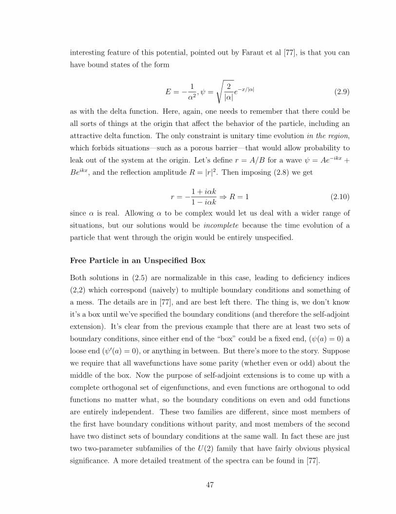
interesting feature of this potential, pointed out by Faraut et al [77], is that you can
have bound states of the form
E = − 1
α2, ψ =
√2
|α|e−x/|α| (2.9)
as with the delta function. Here, again, one needs to remember that there could be
all sorts of things at the origin that affect the behavior of the particle, including an
attractive delta function. The only constraint is unitary time evolution in the region,
which forbids situations—such as a porous barrier—that would allow probability to
leak out of the system at the origin. Let’s define r = A/B for a wave ψ = Ae−ikx +
Beikx, and the reflection amplitude R = |r|2. Then imposing (2.8) we get
r = −1 + iαk
1− iαk⇒ R = 1 (2.10)
since α is real. Allowing α to be complex would let us deal with a wider range of
situations, but our solutions would be incomplete because the time evolution of a
particle that went through the origin would be entirely unspecified.
Free Particle in an Unspecified Box
Both solutions in (2.5) are normalizable in this case, leading to deficiency indices
(2,2) which correspond (naively) to multiple boundary conditions and something of
a mess. The details are in [77], and are best left there. The thing is, we don’t know
it’s a box until we’ve specified the boundary conditions (and therefore the self-adjoint
extension). It’s clear from the previous example that there are at least two sets of
boundary conditions, since either end of the “box” could be a fixed end, (ψ(a) = 0) a
loose end (ψ′(a) = 0), or anything in between. But there’s more to the story. Suppose
we require that all wavefunctions have some parity (whether even or odd) about the
middle of the box. Now the purpose of self-adjoint extensions is to come up with a
complete orthogonal set of eigenfunctions, and even functions are orthogonal to odd
functions no matter what, so the boundary conditions on even and odd functions
are entirely independent. These two families are different, since most members of
the first have boundary conditions without parity, and most members of the second
have two distinct sets of boundary conditions at the same wall. In fact these are just
two two-parameter subfamilies of the U(2) family that have fairly obvious physical
significance. A more detailed treatment of the spectra can be found in [77].
47
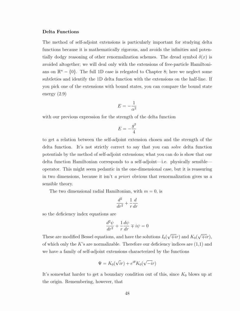
Delta Functions
The method of self-adjoint extensions is particularly important for studying delta
functions because it is mathematically rigorous, and avoids the infinities and poten-
tially dodgy reasoning of other renormalization schemes. The dread symbol δ(x) is
avoided altogether; we will deal only with the extensions of free-particle Hamiltoni-
ans on Rn − 0. The full 1D case is relegated to Chapter 8; here we neglect some
subtleties and identify the 1D delta function with the extensions on the half-line. If
you pick one of the extensions with bound states, you can compare the bound state
energy (2.9)
E = − 1
α2
with our previous expression for the strength of the delta function
E = −g2
4
to get a relation between the self-adjoint extension chosen and the strength of the
delta function. It’s not strictly correct to say that you can solve delta function
potentials by the method of self-adjoint extensions; what you can do is show that our
delta function Hamiltonian corresponds to a self-adjoint—i.e. physically sensible—
operator. This might seem pedantic in the one-dimensional case, but it is reassuring
in two dimensions, because it isn’t a priori obvious that renormalization gives us a
sensible theory.
The two dimensional radial Hamiltonian, with m = 0, is
d2
dr2+
1
r
d
dr
so the deficiency index equations are
d2ψ
dr2+
1
r
dψ
dr∓ iψ = 0
These are modified Bessel equations, and have the solutions I0(√∓ir) and K0(
√∓ir),
of which only the K’s are normalizable. Therefore our deficiency indices are (1,1) and
we have a family of self-adjoint extensions characterized by the functions
Ψ = K0(√ir) + eiθK0(
√−ir)
It’s somewhat harder to get a boundary condition out of this, since K0 blows up at
the origin. Remembering, however, that
48
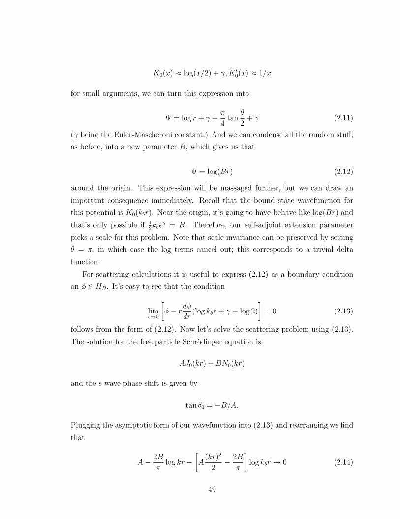
K0(x) ≈ log(x/2) + γ,K ′0(x) ≈ 1/x
for small arguments, we can turn this expression into
Ψ = log r + γ +π
4tan
θ
2+ γ (2.11)
(γ being the Euler-Mascheroni constant.) And we can condense all the random stuff,
as before, into a new parameter B, which gives us that
Ψ = log(Br) (2.12)
around the origin. This expression will be massaged further, but we can draw an
important consequence immediately. Recall that the bound state wavefunction for
this potential is K0(kbr). Near the origin, it’s going to have behave like log(Br) and
that’s only possible if 12kbe
γ = B. Therefore, our self-adjoint extension parameter
picks a scale for this problem. Note that scale invariance can be preserved by setting
θ = π, in which case the log terms cancel out; this corresponds to a trivial delta
function.
For scattering calculations it is useful to express (2.12) as a boundary condition
on φ ∈ HB. It’s easy to see that the condition
limr→0
[φ− r
dφ
dr(log kbr + γ − log 2)
]= 0 (2.13)
follows from the form of (2.12). Now let’s solve the scattering problem using (2.13).
The solution for the free particle Schrodinger equation is
AJ0(kr) +BN0(kr)
and the s-wave phase shift is given by
tan δ0 = −B/A.
Plugging the asymptotic form of our wavefunction into (2.13) and rearranging we find
that
A− 2B
πlog kr −
[A
(kr)2
2− 2B
π
]log kbr → 0 (2.14)
49
and if we drop the second order term this simplifies to
Aπ = 2B log(kb/k) (2.15)
and our phase shift agrees with what we got previously. For m > 0 the free particle
Hamiltonian is self-adjoint, as we’ll see in the next chapter, so a delta function at the
origin can have no impact. The centrifugal barrier shields the particle from seeing the
delta function at all. For the delta function it’s clear enough why this happens: as
you take the cutoff to zero, the repulsive 1/r2 centrifugal potential—which integrates
to ∞ around the origin—drowns out the delta function.
The 3D delta function, from the point of view of self-adjoint extensions, is the
same as the particle on a half-line in the l = 0 channel, since it has the same differen-
tial equation and the same boundary conditions. (The solution using regularization
methods is ψ = e−kr/r, or u(r) = e−kr.) The s-wave phase shift should therefore
be the same as in the 1D case, and it is according to the regularization scheme of
Chapter 1, so once again we’re consistent.
As we will see in the next chapter, all delta functions are self-adjoint in the l > 0
channels.
Fall to the Center
Consider the classical two-body problem with V (r) = ρ/r2. This potential just
modifies the centrifugal barrier term, and when it is repulsive or weaker than the
barrier term the problem is well-behaved. However, if it is strong enough to overcome
the centrifugal barrier, the particle falls to the origin in a finite time, and its behavior
after that point is not well-defined. The general equation of motion is (Thornton and
Marion [82], 8.20)
d2u
dθ2+ u = − µ
l2u2F (1/u) (2.16)
where u = 1/r. As Thornton shows (Example 8.1), an inverse square potential
(equivalently an inverse cube force) leads to solutions of the form
r = Ae−kθ +Bekθ (2.17)
for some constant k. Evidently, there are no periodic combinations of these solutions,
so the particle must spiral in or out. The solution that spirals outwards is not inter-
esting; the important thing about the inward spiral is that as the particle approaches
50
the origin, its velocity must be infinite to conserve angular momentum. We can see
this directly from Thornton’s expression for the radial velocity:
r =
√E − U − l2
r2. (2.18)
In our case, this is
r =
√E +
λeffr2
.
As the particle approaches the origin this expression blows up. If we separate the
equation and integrate, we see that
tf − ti =
∫ R
0
dr√E +
λeff
r2
∝√
1 +R2 (2.19)
so any particle reaches the origin with an infinite velocity in a finite time. This
phenomenon is known as fall to the center. The equations of motion cease to be well-
defined when the particle reaches the origin, and therefore our solution doesn’t work
for all time. Solutions of this type are called classically incomplete. On quantizing
the theory this turns into a failure of unitary time evolution, and therefore of self-
adjointness. However, as Ref. [19] points out, one could make the classical theory
well-defined for all time by requiring that the particle be reflected whenever it gets to
the origin—i.e. running our time evolution forwards and backwards endlessly. This
corresponds, in the quantum problem, to picking a self-adjoint extension.
Note that there’s a slight subtlety here. Mildly singular quantum mechanical
problems are regular even in the l = 0 channel, whereas classically they collide with
the origin after a finite time. In general, the “centrifugal potential” (the l term) in
quantum mechanics works quite differently from its classical counterpart; this is why
it’s misleading to think of the critical value of the 1/r2 potential (see Chapter 3) as
the point at which the particle overcomes the centrifugal barrier.
Because of the importance of singular potentials, I will leave the quantum me-
chanical treatment to a later chapter, noting only that the deficiency indices are (1,1)
as we’d expect (one boundary condition at the origin).
Fall to Infinity
Consider the classical 1D Hamiltonian
51
H =p2
2− q4. (2.20)
By Hamilton’s equations,
q =∂H
∂p= 2p.
Since the total energy E = H is conserved, we can rewrite this as the relation
E = q2 − q4 (2.21)
which can be rearranged to give
dq
dt=√E + q4. (2.22)
Solving this equation for t, we find that
tf − ti =
∫ qf
qi
dq√E + q4
. (2.23)
For a particle with E > 0 this integral converges from −∞ to ∞, so any particle
reaches infinity in a bounded time, and the solution is not complete. In fact, we need
to add two boundary conditions—reflection at ∞ and at −∞—to make the solution
complete.
One might expect the same result to hold for the upside down oscillator:
H = p2 − q2. (2.24)
However, the integral in this case,
tf − ti =
∫ qf
qi
dq√E + q2
= sinh−1 qf/√E − sinh−1 qi/
√E (2.25)
does not converge, and we have a complete classical solution.
As you might expect, these potentials have deficiency indices (2,2) and (0,0) re-
spectively. In general, power-law potentials are classically complete if and only if
they are quantum mechanically complete. However, this is not generally true of quan-
tum mechanical potentials. There are exceptions to this rule both ways, given in [75].
An interesting one is the following potential, a bottomless hill with increasingly tall
and narrow spikes at integer values of x:
52
V (x) = −x4 + g(x)
g(x) = |N |, | x−N | < 1/N.
This is classically complete, since a particle of any energy eventually runs into
a sufficiently tall barrier. However, the quantum mechanical problem is still patho-
logical, because a particle can tunnel through all the barriers. Similarly, the delta
function is classically well-behaved since it has zero range and nothing scatters off
it; however, wavefunctions are spread-out so it has a nontrivial quantum mechanical
scattering range, which needs to be specified by picking a self-adjoint extension.
A useful general result due to Weyl is the following:
Theorem 6 (Weyl) A Hamiltonian of the form
H = − d2
dx2+ V (x)
is essentially self-adjoint on (0,∞) iff the equation Hψ = iψ has at least one solution
that fails to be square integrable near zero, and at least one solution (possibly the same
one) that fails to be square integrable near infinity.
The forward direction is trivial from the definitions; the reverse is proved in Reed
and Simon (X.7). This result makes life a little simpler in some cases because we
can treat short-range and long-range singularities as independent. If there’s only one
solution at 0 (∞), the potential is said to be limit point at 0 (∞); otherwise it’s
said to be limit circle. The terms are basically conventional.
2.5 Boundedness and the Friedrichs Extension
An upper semi-bounded operator A has the property that for functions in its
domain, (φ,Aφ) ≥ c‖φ‖, where c ∈ R is a fixed number. Most operators that we deal
with in physics have this property; it is basically the same thing as requiring that the
system have a ground state. Most operators are not bounded above; for instance the
harmonic oscillator has arbitrarily high bound states, and so does any operator with
a scattering sector. On the other hand, we have seen two instances of operators that
are bounded neither above nor below—attractive singular potentials and upside down
53
polynomials. These operators are fundamentally unbounded, in that the Hamiltonian
itself has no lower bound. On the other hand, in cases like the 2D delta function, it is
only the adjoint that is unbounded from below, and picking a self-adjoint extension
bounds the operator.
Most of quantum mechanics is done with the assumption of semiboundedness,
however, and the particular extension that is typically picked out is the Friedrichs
extension. A rough and ready way to obtain the Friedrichs extension on a domain
D is by imposing the boundary condition ψ(x) = 0 on all x ∈ ∂D. This is the
correct boundary condition for most cases that we are interested in: the particle in a
box, the 3D Coulomb problem, and so on. But sometimes, as with δ(x), there might
be a specific motivation for choosing a non-Friedrichs extension, and sometimes—
e.g. one-dimensional quantum mechanics, discussed later—the Friedrichs extension
is blatantly unphysical, and leads to strange spectra.
There are two subtleties with the Friedrichs extension that show up in later chap-
ters. The first has to do with the free-particle Hamiltonian in two dimensions, for
which neither solution vanishes at the origin, and the second, with the weakly attrac-
tive 1/r2 problem in one dimension, for which both solutions vanish at the origin.
In the second case, if one substitutes v(r) = u(r)/√r, one gets a new differential
equation for which only one of the solutions vanishes. The Friedrichs extension of the
substituted differential equation is also the Friedrichs extension of the original differ-
ential equation. However, in general, even when the Friedrichs extension doesn’t set
all boundary conditions to zero, it is the extension that corresponds to throwing out
the more singular solution.
Friedrichs extensions are defined only for semibounded Hamiltonians; if the origi-
nal Hamiltonian is unbounded from below, then so are all self-adjoint extensions, and
there is no Friedrichs extension.
2.6 Rigged Hilbert Space Formalism
(The introductory material follows Refs. [79] and [83].) To understand the need2 for
a rigged Hilbert space, consider an operator like x. This is a self-adjoint operator, and
we are used to saying that a self-adjoint operator has a complete set of eigenvalues,
but x in fact has no eigenvalues, since the formal solutions δ(x − λ) are not in the
2Or what some consider the need.
54
Hilbert space. Similarly, a Schrodinger operator with a continuous spectrum, such
as H = −∇2, has no eigenvalues in the Hilbert space, and the square well has only
a few. The rest of the spectrum is normally accounted for by means of projection
operators and the spectral theorem ([71]). The rigged Hilbert space is an expanded
Hilbert space that includes several non-normalizable solutions.
The rigged space is constructed as follows. We first construct a nuclear space
Ω, which is a subset of the Hilbert space. Recall that the Hilbert space contains all
convergent sums of Fourier series. Now Ω includes only those sums that have the
property that for all positive m, ∑n
|cn|2nm <∞.
A continuous version of this might be∫ ∞
0
|ψ|2xmdx <∞
and in fact de la Madrid [83] derives the nuclear space from the requirement that
wavefunctions in it should be in the domain of the operators xm and pm for all m.
The space we are really interested in is ΩD, the dual space of Ω, or the space
of all linear functionals f : Ω → C. The correct way to think of a dual space is as
a one-sided inner product: ΩD consists of all the bras that are well-behaved with
respect to the kets in Ω. The stronger the restrictions on the kets, the more bras we
are likely to find that work, so one would expect ΩD ⊇ H ⊇ Ω. H is special in that
H = HD.
In fact, because wavefunctions in Ω are required to vanish so much more rapidly
than in H, the continuous spectrum is normally in ΩD. This is the basis of the
generalized spectral theorem, which is the key to interest in rigged Hilbert spaces:
Theorem 7 (Generalized Spectral Theorem) A self-adjoint operator has a com-
plete set of eigenfunctions in the rigged Hilbert space.
The theory just outlined raises a few questions about our understanding of self-
adjoint extensions. For instance, if, as de la Madrid claims, the nuclear space Ω is the
physical sector of the Hilbert space, it follows that self-adjoint extensions introduce
new physics only if they have some impact on members of Ω. But this implies that Ω
should never be a subset of a non-self-adjoint original domain DH . If this is true, then
55
(since self-adjoint extensions affect a domain by throwing out several states in the
adjoint domain) there must be vectors in Ω that didn’t make it to DHθ. Therefore, Ω
consists of more than just physically meaningful states, since functions outside DHθ
are physically irrelevant.
Besides, this raises the question of what happens if the momentum operator fails
to be self-adjoint: can one still define a rigged Hilbert space from the physicality
requirement? We have not had the time to address these questions, but they seem
relevant if the nuclear space is to be interpreted in physical terms.
56
Chapter 3
Singular Potentials
Singular potentials are poorly behaved in classical mechanics too, as we saw in the
previous chapter, but at least one has a fairly good physical idea of what is going
on there. In quantum mechanics, this is somewhat harder to obtain. In some ways
the cleanest way to look at singular potentials is through the formal apparatus of
Chapter 2, so that’s what we’ll do first. We focus on the inverse square potential, not
because it’s the most typical case (it isn’t), but because it is exactly solvable.
3.1 The Inverse Square Potential
The 3D radial Schrodinger equation looks like this:
−d2u
dr2+λ
r2u+
l(l + 1)
r2u = k2u (3.1)
in terms of u(r) = ψ/r. This substitution is convenient because it makes the 3D
problem look like a 1D problem. It’s especially convenient that the space of functions
u : (0,∞) → C corresponding to ψ ∈ L2(R3) is almost exactly L2(0,∞) because the
1/r’s cancel the spherical Jacobian. The additional constraint [79] is that usually we
enforce u(0) = 0 to have the wavefunction be regular at the origin. This constraint
leads to some of the important differences between 3D and 1D quantum mechanics,
e.g. the fact that 3D square wells do not always have bound states; however, we shall
sometimes have reason to relax it.
With an inverse square potential, the “one-dimensional” Hamiltonian becomes
H = − d2
dr2+λ
r2+l(l + 1)
r2= − d2
dr2+λeffr2
(3.2)
57
Since—as investigators of EFTs—we are most interested in low-energy aspects of
this problem we shall normally have l = 0, and for simplicity we shall generally write
λeff as λ. The eigenfunctions of (3.2) can be expressed in terms of Bessel functions
as follows:
√rZζ+1/2(kr)
where
ζ(ζ + 1) = λ. (3.3)
Now we’d like to use Weyl’s result to check for self-adjointness. The eigenfunctions
corresponding to i are√rIζ+1/2(
√ir) and
√rKζ+1/2(
√ir). As r → ∞, we can see
from the asymptotic expansions
Iν(z) ∼ez√z⇒ |Iν(x+ iy)| ∼ ex√
x
Kν(z) ∼e−z√z⇒ |Kν(x+ iy)| ∼ e−x√
x
that for any ζ, we always have exactly one integrable solution at∞. At zero, however,
the expansions are:
Iν(z) ∼ zν ;Kν(z) ∼ z−ν .
Depending on ζ, we could have three different situations. The boundary between
the first two is based on integrability of bound state wavefunctions; the more drastic
change in behavior takes place when the discriminant of (3.3) changes sign and ζ
becomes complex.
3.2 Strongly Repulsive Regime (λ ≥ 34, ζ ≥
12)
Kζ+1/2(√ir) ∼ r−(ζ+1/2) (3.4)
The solution with K fails to be square integrable at the origin because
|r1/2Kζ+1/2(√ir)|2 ∼ r−2ζ (3.5)
which is more singular than 1/r at the origin. Therefore, by Weyl’s theorem, the
Hamiltonian is self-adjoint.
58
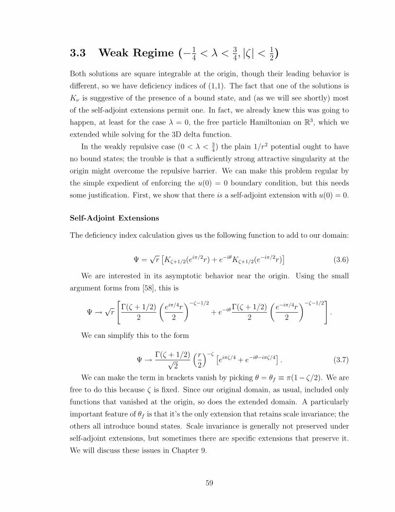
3.3 Weak Regime (−14 < λ < 3
4, |ζ| <12)
Both solutions are square integrable at the origin, though their leading behavior is
different, so we have deficiency indices of (1,1). The fact that one of the solutions is
Kν is suggestive of the presence of a bound state, and (as we will see shortly) most
of the self-adjoint extensions permit one. In fact, we already knew this was going to
happen, at least for the case λ = 0, the free particle Hamiltonian on R3, which we
extended while solving for the 3D delta function.
In the weakly repulsive case (0 < λ < 34) the plain 1/r2 potential ought to have
no bound states; the trouble is that a sufficiently strong attractive singularity at the
origin might overcome the repulsive barrier. We can make this problem regular by
the simple expedient of enforcing the u(0) = 0 boundary condition, but this needs
some justification. First, we show that there is a self-adjoint extension with u(0) = 0.
Self-Adjoint Extensions
The deficiency index calculation gives us the following function to add to our domain:
Ψ =√r[Kζ+1/2(e
iπ/2r) + e−iθKζ+1/2(e−iπ/2r)
](3.6)
We are interested in its asymptotic behavior near the origin. Using the small
argument forms from [58], this is
Ψ →√r
[Γ(ζ + 1/2)
2
(eiπ/4r
2
)−ζ−1/2
+ e−iθΓ(ζ + 1/2)
2
(e−iπ/4r
2
)−ζ−1/2].
We can simplify this to the form
Ψ → Γ(ζ + 1/2)√2
(r2
)−ζ [eiπζ/4 + e−iθ−iπζ/4
]. (3.7)
We can make the term in brackets vanish by picking θ = θf ≡ π(1− ζ/2). We are
free to do this because ζ is fixed. Since our original domain, as usual, included only
functions that vanished at the origin, so does the extended domain. A particularly
important feature of θf is that it’s the only extension that retains scale invariance; the
others all introduce bound states. Scale invariance is generally not preserved under
self-adjoint extensions, but sometimes there are specific extensions that preserve it.
We will discuss these issues in Chapter 9.
59
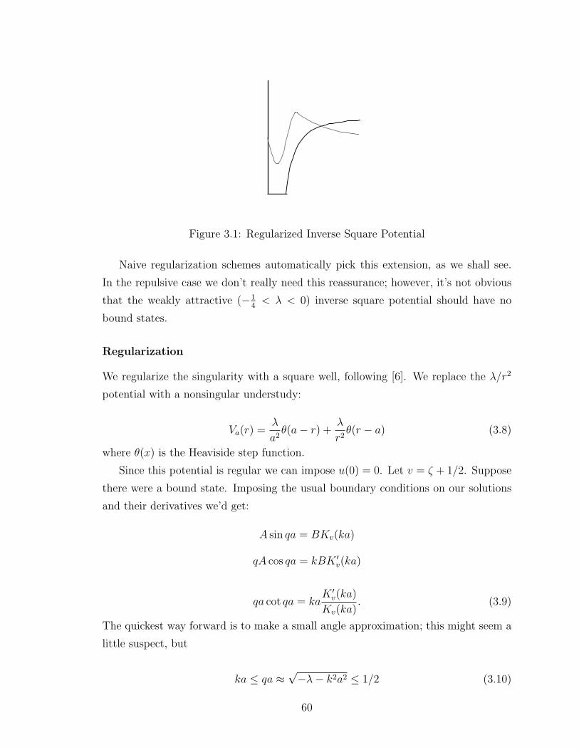
Figure 3.1: Regularized Inverse Square Potential
Naive regularization schemes automatically pick this extension, as we shall see.
In the repulsive case we don’t really need this reassurance; however, it’s not obvious
that the weakly attractive (−14< λ < 0) inverse square potential should have no
bound states.
Regularization
We regularize the singularity with a square well, following [6]. We replace the λ/r2
potential with a nonsingular understudy:
Va(r) =λ
a2θ(a− r) +
λ
r2θ(r − a) (3.8)
where θ(x) is the Heaviside step function.
Since this potential is regular we can impose u(0) = 0. Let v = ζ + 1/2. Suppose
there were a bound state. Imposing the usual boundary conditions on our solutions
and their derivatives we’d get:
A sin qa = BKv(ka)
qA cos qa = kBK ′v(ka)
qa cot qa = kaK ′v(ka)
Kv(ka). (3.9)
The quickest way forward is to make a small angle approximation; this might seem a
little suspect, but
ka ≤ qa ≈√−λ− k2a2 ≤ 1/2 (3.10)
60
and while this might not seem like a sufficiently tight constraint, 1/2 is actually a
pretty small angle—sufficiently small that first-order terms dominate the behavior of
the trig functions. Expanding out both sides,
1 = ka(−v/2)(ka/2)−v−1
(ka/2)−v⇒ 1 = −v (3.11)
and this is inconsistent, so there can be no bound states. This treatment might
be somewhat sloppy, but it’s valid for small λ at any rate, and is meant merely
to provide a heuristic justification for picking the Friedrichs extension. A hand-
wavy mathematical reason for picking the Friedrichs extension over this domain is
as follows. The problem is analytic in λ on (−14, 0), and there are no singularities
or zeros of cot qa, so we don’t expect θ (or the number of bound states) to behave
non-analytically in λ. Since θ = θf on (−e, 0) ⊆ (−14, 0) for some e, it should be
constant for all e.
There’s a tighter argument in Radin’s paper [22]. Radin also observes that the
regularized theory has singularities only in the l = 0 sector. One of the flaws of earlier
treatments is that they regularize the centrifugal barrier term as well as the potential;
Radin conscientiously avoids this.
The boundary between weak and strong regimes at λ = −1/4 is still weak, but
has a slight calculational subtlety.
3.4 Critical Value (λ = −14)
Since the treatments of the next chapter come down to solving this regime, it is of
some historical importance. The solution of the weak regime isn’t directly applicable
here, because both solutions go as√r, and we’re missing one independent solution.
A way to see what’s going on is to notice that the Schrodinger equation, under the
transformation v(r) = u(r)/√r, is exactly the free Bessel equation in two dimensions.
(This is no accident, see the definition of spherical Bessel functions in [56].) The
independent solutions are therefore√krK0(kr) ∼
√kr log kr and
√krI0(kr) ∼
√kr.
We could take the Friedrichs extension, throw out the K0 solution, and retain scale
invariance, so we aren’t yet in the strong regime.
61
3.5 Strongly Attractive Regime (λ < −14)
Solving (3.3) for ζ, we get
ζ = −1
2±√λ+
1
4. (3.12)
In this regime, the square root is imaginary; let’s call it iΞ. The solutions to
Schrodinger’s equation are now
√krZ±iΞ(kr)
All Bessel functions of nonzero order have the behavior Zv(x) ∼ x±v at the origin.
This means that that they either blow up or vanish at the origin as long as <(v) 6= 0,
but when <(v) = 0,
x±iy = e±iy log x = cos(y log x)± i sin(y log x)
The solutions differ from each other by a phase, but the phase isn’t even well-defined
at the origin, since both solutions are oscillating infinitely rapidly there. Since all
solutions of this form are certainly integrable near the origin, we have deficiency
indices (1,1), and a one-parameter family of self-adjoint extensions, which select the
phase. We can pick the correct self-adjoint extension by the same method as before,
and we do this a few sections down, but there is a simpler procedure due to Case [1].
Case’s Way
The failure of self-adjointness manifests itself very dramatically in the fact that every
negative energy has an eigenfunction. With most potentials the boundary conditions
keep the bound state spectrum discrete by forbidding most energies. However, with
our potential, KiΞ is always sufficiently well-behaved at infinity and at the origin.
Near the origin it goes like
√r cos(Ξ log(kr) +B),
where B is energy-independent. We can rewrite this, with our usual abuse of notation,
as
cos[Ξ log r + (B + Ξ log k)] = cos(log r +B′) (3.13)
62
and this behaves the same way for all energies at the origin, because log r blows up.
Evidently, this violates orthogonality, since functions for infinitesimally separated k
look alike and certainly are not orthogonal. However, we can restore orthogonality
by hand, as Case does, by the following procedure. Consider the two Schrodinger
equations
D2ψ1 +
[λ
r2− k2
1
]ψ1 = 0
D2ψ2 +
[λ
r2− k2
2
]ψ2 = 0.
(The derivative commutes with complex conjugation.) If we multiply the first equa-
tion by ψ2 and the second by ψ1, and then subtract, the inverse-square term cancels.
This leaves us with the following equation
ψ1d2ψ2
dr2− d2ψ1
dr2ψ2 = (k2
1 − k22)ψ1ψ2. (3.14)
If we integrate this over all space, the rhs becomes
(k21 − k2
2)
∫ ∞
0
ψ1ψ2 dx = (k21 − k2
2)(ψ2, ψ1).
To have orthogonality, therefore, the integral over all space of the lhs must be zero.
Since
(fg′)′ = f ′g′ + fg′′
we can simplify the integrand on the lhs to
(ψ1ψ′2)′ − (ψ′1ψ2)
′
and use the fundamental theorem of calculus to get the following condition:[ψ1dψ2
dr− ψ2
dψ1
dr
]∞0
= 0. (3.15)
Since everything vanishes at ∞ because of the exponential falloff of KiΞ, all we
need is equality at zero. Plugging in the small-argument form (3.13) and simplifying,
we find the constraint:
sin(B′2 −B′
1) = 0. (3.16)
63
In terms of the energy-dependent phase this equation implies
Ξ(log ka − log kb) = nπ (3.17)
and the bound state separation is given by
kakb
= enπ/Ξ. (3.18)
Fixing any one of the bound state energies determines the entire spectrum, and—
as we expect—specifies a self-adjoint extension of the Hamiltonian. The bizarre thing
about this spectrum is that it is unbounded from below, since n can be either positive
or negative; there are infinitely many bound states going all the way up to 0 and all
the way down to −∞. Case dismissed the potential as unphysical for this reason, but
it might still be useful from an effective field theory point of view because deep bound
states are not obviously low-energy observables. In fact, as Refs. [30], [32] show, if
we regularize the potential with a square well or a delta function ring of radius a, we
can take a→ 0 without affecting the shallow bound states at all. The accumulation
of bound states at E = 0 is a result of the long-range nature of this potential, and
can be avoided—as with the hydrogen atom—by cutting off the potential at large
distances.
3.6 Singularity vs. Anomaly
The literature on the inverse square potential has two threads—one addresses its
pathologies as a result of scale invariance, the other, as consequences of fall to the
center. Pathologies like a continuum of bound states might seem characteristic of
scale invariant potentials. However, let’s look at the close-in behavior of potentials
more singular than 1/r2.1 These are generally not analytically solvable; however, we
can still investigate the behavior near the origin, since, in the Schrodinger equation
u′′(r) =(k2 − α
rn
)the energy k2 becomes negligible as r → 0. So we solve the simpler equation
Hψ = 0. (3.19)
1With highly singular potentials there is no qualitative difference between the 1D and 3D prob-
lems, so I’ll switch back and forth at will.
64
The solutions to this equation are called zero-energy wavefunctions, and are very
helpful in the study of singular potentials. In general the two independent solutions
to the zero-energy equation
d2u
dr2+α
rnu(r) = 0 (3.20)
can be written as follows:
u(0, r) ∼√r[(AJ1/(n−2)
(r(2−n)/2
)+BJ−1/(n−2)
(r(2−n)/2
)]. (3.21)
There is a particularly nice solution for n = 4:
u(0, r) = x cos
(√α
r+B
). (3.22)
(3.21) oscillates wildly near the origin for n < −2, and all solutions of form (3.22)
behave the same way at the origin because the phase is negligible compared with the
singularity in r. So, once again, we have a failure of self-adjointness and a continuum
of bound states. The fix a la Case is the same as before, since the derivation in the
previous section holds for basically arbitrary f(x) in place of sin(log x). However, we
get less information out of the condition on B than we formerly did. In particular,
without a solution to the actual Schrodinger equation, we can’t get much information
about the eigenvalues and their spacing. For E → −∞, Perelomov [20] uses the
quasiclassical approximation to obtain
EkE0
= k2N/(N−2) (3.23)
for the 1/rN potential. However, this is not the sector we are interested in. The
case N = 4 is slightly better than others because Schrodinger’s equation is exactly
solvable in terms of Mathieu functions [12]. The asymptotic form of the solution near
the origin is
φ(r) → r cos
(√α
r− νπ
2+ χ
)(3.24)
where ν is (in the words of Ref. [12]) a “very complicated function” with a less
than straightforward dependence on k. The presence of energy-dependent phases
was expected; however, the relation is sufficiently unpleasant that we have no hope of
getting a simple general expression for the energy level spacing. An interesting feature
of this problem is the way both short-distance and long-distance length scales enter
65
into the treatment—the levels are determined by ν, which depends on k, therefore
on the self-adjoint extension, and finally on the short-distance physics; however, the
frequency of oscillation near the origin is determined by the “intrinsic scale” of α.
This is an example of when dimensional analysis breaks down, since there are two
entirely different scales that influence both long-distance and short-distance behavior.
That multiple scales are necessary can be seen from the following dimensional
argument. The coupling of the g/rn potential is a positive power of inverse length
(i.e. an energy) for n < 2, but a positive power of length for n > 2. Suppose n > 2,
and g is the only scale. Then the magnitude B of the ground state energy must
scale with g. Since g is a length and B is an inverse length, it follows that B must
decrease as the coupling increases; that is, the ground state must get shallower as the
potential well becomes deeper. This doesn’t make physical sense, and the only way
to rescue the situation is to put the ground state at −∞, or to introduce a new scale
using self-adjoint extensions or renormalization.
With weakly singular potentials like 1/r, the coupling is an energy, so the ground
state energy scales as it should. However, the scattering length is an inverse energy,
so it should decrease as the coupling increases. Again, this makes no sense, and the
only way out is for the scattering length to be infinite.
Something that Newton [62] considered terminally weird about the 1/r4 and more
singular attractive potentials, is that for these the full 3D Schrodinger equation has
no solutions at all. The pathology is essentially the same as that of the point source
in electrostatics.
∇2(1/r) = −4πδ3(r) 6= 0.
It has been shown in the literature ([62],[11]) that the correct radial part of the
Hamiltonian in this case is
∂2
∂r2+
2
r
∂
∂r+ δ(r)
∂
∂r
so that our correct radial Schrodinger equation has an extra term, which looks like
a δ′ potential. Newton used this as an excuse to dismiss the potential as unphysi-
cal; however, to our EFT-indoctrinated minds, all this shows is that some form of
renormalization is essential.
We’ll consider the 1/r4 potential again, in the context of limit cycles, but the
point of this detour was to point out that at least some of the features of the 1/r2
potential are shared with potentials that are not scale-invariant.
66

3.7 Non-Friedrichs Extensions of the 1/r2 Poten-
tial
Case’s method is quite broadly applicable as a way of doing self-adjoint extensions.
For example, we could use it to solve the two-dimensional delta function. Suppose
we fix a bound state kb. Because the particle is free except at the origin, this would
have to have the wavefunction K0(kbr). Suppose there were another (m = 0) bound
state, ks. It would also have to have the wavefunction K0(ksr) almost everywhere.
Both wavefunctions are nodeless and always positive, so∫ ∞
0
K0(kbr)K0(ksr) ≥ 0
and the states cannot be orthogonal, so the operator cannot be self-adjoint. This tells
us that there’s at most one bound state with arbitrary energy.
However, a limitation of Case’s method is that it doesn’t tell us about the Friedrichs
extension, or about extensions without bound states. In particular, it does not tell us
a very important thing about the 1/r2 potential, which is that the Friedrichs exten-
sion ceases to exist for λ < −1/4. This is important because it shows that—unlike
the “2D delta function,” which has an anomaly only because it’s defined as an exten-
sion with an anomaly—anomalous symmetry breaking is inevitable for a strong 1/r2
potential.
This section treats the inverse square potential using the apparatus of self-adjoint
extensions that we developed in the previous chapter. The expressions obtained here
are used in later chapters; however, the algebra is unpleasant and not dissimilar to
what we did in Chapter 2.
3.7.1 One Dimension
In the regime −1/4 < λ < 3/4, both solutions to the Schrodinger equation are
square-integrable at the origin, so probability conservation is no longer adequate to
distinguish between them. Let λ = ζ(ζ+1); then the regular and less regular solutions
go as xζ+1 and x−ζ near the origin respectively. As λ decreases and becomes negative,
the regularity gap between the two solutions closes; for λ < 0 both functions vanish
at the origin. For λ = 0 the irregular solution is a constant, like e−kx or cos kx; this
is the case of δ(x). For λ = −1/4 the irregular solution is√kxK0(kx), which goes as
√x log x; the regular solution is
√x.
67
The attractive region is weird because neither of the solutions behaves as one would
expect: for both solutions, ψ(0) = 0 and the derivative has an infinite discontinuity.
(The latter feature is shared with the one-dimensional Coulomb potential, see Chapter
8.)
Energies and Extensions
To a better approximation than (3.3), the small-argument form of (3.6) is
ψ ∼ x1+ζf(ζ)[eiπζ/4 + ei(θ−πζ/4)
]+ x−ζg(ζ)
[ei(θ+πζ/4) + e−iπζ/4
]. (3.25)
If we rewrite this as
ψ ∼ Ar1+ζ +Br−ζ
we can rearrange it to read
ζψ + xψ′
(1 + ζ)ψ − xψ′=A
Bx1+2ζ . (3.26)
The effective length scale is set by A/B, which has dimensions k1+2ζ and is a function
of θ. We could work this out explicitly with gamma-function identities, but it’s
simpler in this case to point out that, by tweaking θ, we can have A = 0, B 6= 0
and vice versa. Absorbing the θ-dependence into our length scale, we get a boundary
condition of the form
ζψ + rψ′
(1 + ζ)ψ − rψ′= F (ζ)(κr)1+2ζ (3.27)
where β is an arbitrary constant, and |κ| ∈ (0,∞) parameterizes the extension chosen.
If we plug in a bound state of the form√kbxKζ+1/2(kbx), we swiftly discover that
F (ζ) =Γ(−ζ − 1/2)
Γ(ζ + 1/2)
so the bound state energy is proportional to κ, as we expect, and our final boundary
condition is
ζψ + xψ′
(1 + ζ)ψ − xψ′=
Γ(−ζ − 1/2)
Γ(ζ + 1/2)(kbx)
1+2ζ . (3.28)
68
This is a useful form for the boundary condition, because it’s cast solely in terms of ob-
servables and the long-distance coupling. We can derive the s-wave phase shift by ap-
plying the boundary condition to a scattering state,√kx(AJζ+1/2(kr)+BNζ+1/2(kr)).
The leading behavior of scattering states is
Jν ∼(kr
2
)ν1
Γ(1 + ν)
Nν ∼1
πΓ(ν)
(kr
2
)−ν+
cos πν
πΓ(−ν).
(kr
2
)νApplying the boundary condition to this gives
Aπ +B cos[π(ζ + 1/2)]Γ(−ζ − 1/2)Γ(ζ + 3/2)
BΓ(ζ + 1/2)Γ(ζ + 3/2)
(kr
2
)1+2ζ
=Γ(−ζ − 1/2)
Γ(ζ + 1/2)
(kbr
2
)1+2ζ
(3.29)
which looks slightly less unpleasant rearranged:
B
A=
π
Γ(ζ + 3/2)Γ(−ζ − 1/2)
1
cos[π(ζ + 1/2)]− (k/kb)1+2ζ. (3.30)
(Let’s write ν = ζ + 1/2.) One further simplification comes from the reflection
formula Γ(12+ z)Γ(1
2− z) = π sec πz. For us, z = ν+1/2, we get the expression down
to
B
A=
cos[π(ν + 1/2)]
cos πν − (k/kb)2ν. (3.31)
Now B/A is a quantity related to the l = 0 phase shift; its dependence on k breaks
scale invariance, and we have (once again) an anomaly.
The scattering phase shifts of the 1/x2 potential are a little tricky because, like
the Coulomb potential, it’s a long-range interaction and the asymptotic forms are√kxZζ+1/2(kx) rather than eikx. It’s slightly easier because the Bessel functions are
just phase-shifted sines and cosines (AS 9.2.3). (Henceforth we’re going to write
ζ + 1/2 = ν.)
√kxJν(kx) = cos
(kx− πν
2− π
4
)√kxNν(kx) = sin
(kx− πν
2− π
4
).
And one can check that
69
A√kxJν(kx) +B
√kxNν(kx) ∼ C cos
(kx− πν
2− π
4− tan−1 B
A
). (3.32)
Because of Levinson’s theorem [62], which we discuss later, we expect the phase shift
at k = kb to be π/2. Let’s check this. 3.31 simplifies to
B
A=
cos[π(ν + 1/2)]
cos πν − 1. (3.33)
With the help of two well-known trig identities one can get this down to
B
A= − cot(πν/2)
which means that
tanB
A=πν
2− π
2.
Putting this back into 3.32 we see that
√kx(AJν(kx) +BNν(kx)) ∼ C cos
(kx+
π
4
). (3.34)
This is not quite what we expect from a normal potential. However, if we look at the
behavior of 3.31 at very high energies, B/A = 0, and the phase shift is −(πν2
+ π4)
rather than 0, as we have been bred to expect.
3.7.2 Two Dimensions
In two dimensions with m = 0, the bound-states Schrodinger equation with a 1/r2
potential is
r2d2ψ
dr2+ r
dψ
dr± k2r2 + λψ = 0 (3.35)
and the solutions to this are simply the relevant Bessel functions Zν(kr), where ν =√λ. So everything goes pretty much as in the 1D and 3D cases, except for the
clutter of√kr terms. The self-adjointness calculation is more straightforward in two
dimensions, but the details are similar enough to be beneath repetition.
νψ + rψ′
νψ − rψ′=
(βr
2
)2ν
(3.36)
70

where β is a parameter related to the self-adjoint extension and the bound state
energy. This sets us up to calculate an energy dependent scattering phase shift, as we
did in one dimension. We can replace β with a bound state energy as we did before,
and get
νψ + rψ′
νψ − rψ′=
Γ(−ν)Γ(ν)
(kbr
2
)2ν
. (3.37)
Plugging in the general scattering solution, which is AJν(kr) + BNν(kr), we get
3.31 once again. The treatment of scattering works identically, except that in 2D
scattering [60] we don’t subtract the π/4, since it’s built into the asymptotic forms of
the Bessel functions. Therefore the phase shift at k = kb is π/2, which is consistent
with Levinson’s theorem.
Now let’s do the same calculation in the strong regime. First of all, the equivalent
of 3.25 is
ψ ∼ xiνf(ν)[e−πν/4 + ei(θ−iπν/4)
]+ x−iνg(ν)
[ei(θ+iπν/4) + eπν/4
](3.38)
Since x±iν look the same at the origin, there isn’t a preferred extension. Setting a
phase between the two solutions means introducing arbitrary new physics, but that’d
be true in some sense even if there were a Friedrichs extension: the special thing about
the Friedrichs extension is that by throwing out one of the states altogether, we can
escape the anomaly. We would avoid the anomaly, even here, if we could arbitrarily
throw out one of the solutions. However, if we look at the ratio of the coefficients in
this case (leaving out stuff independent of θ), it is
Π1
Π2
=e−iθ/2e−πν/4 + eiθ/2eπν/4
eiθ/2e−πν/4 + e−iθ/2eπν/4
and since the numerator and denominator are conjugates, |Π1/Π2| = 1 and the solu-
tion with vanishing x±iν is not a self-adjoint extension, so there is absolutely no way
to preserve scale invariance.
The rest of the self-adjointness calculation goes the same way it did before,
iνψ + rψ′
iνψ − rψ′=
(βr
2
)2iν
= e2iν logBr (3.39)
or, in terms of a bound state energy,
71
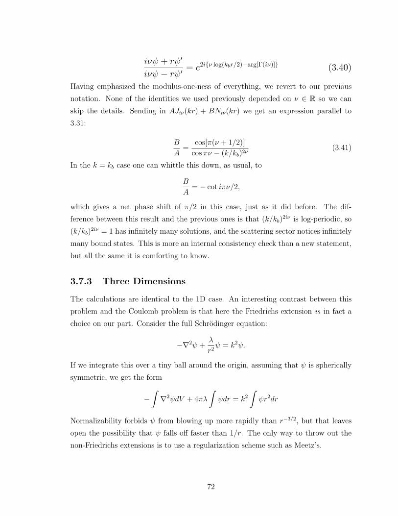
iνψ + rψ′
iνψ − rψ′= e2iν log(kbr/2)−arg[Γ(iν)] (3.40)
Having emphasized the modulus-one-ness of everything, we revert to our previous
notation. None of the identities we used previously depended on ν ∈ R so we can
skip the details. Sending in AJiν(kr) + BNiν(kr) we get an expression parallel to
3.31:
B
A=
cos[π(ν + 1/2)]
cos πν − (k/kb)2ν(3.41)
In the k = kb case one can whittle this down, as usual, to
B
A= − cot iπν/2,
which gives a net phase shift of π/2 in this case, just as it did before. The dif-
ference between this result and the previous ones is that (k/kb)2iν is log-periodic, so
(k/kb)2iν = 1 has infinitely many solutions, and the scattering sector notices infinitely
many bound states. This is more an internal consistency check than a new statement,
but all the same it is comforting to know.
3.7.3 Three Dimensions
The calculations are identical to the 1D case. An interesting contrast between this
problem and the Coulomb problem is that here the Friedrichs extension is in fact a
choice on our part. Consider the full Schrodinger equation:
−∇2ψ +λ
r2ψ = k2ψ.
If we integrate this over a tiny ball around the origin, assuming that ψ is spherically
symmetric, we get the form
−∫∇2ψdV + 4πλ
∫ψdr = k2
∫ψr2dr
Normalizability forbids ψ from blowing up more rapidly than r−3/2, but that leaves
open the possibility that ψ falls off faster than 1/r. The only way to throw out the
non-Friedrichs extensions is to use a regularization scheme such as Meetz’s.
72
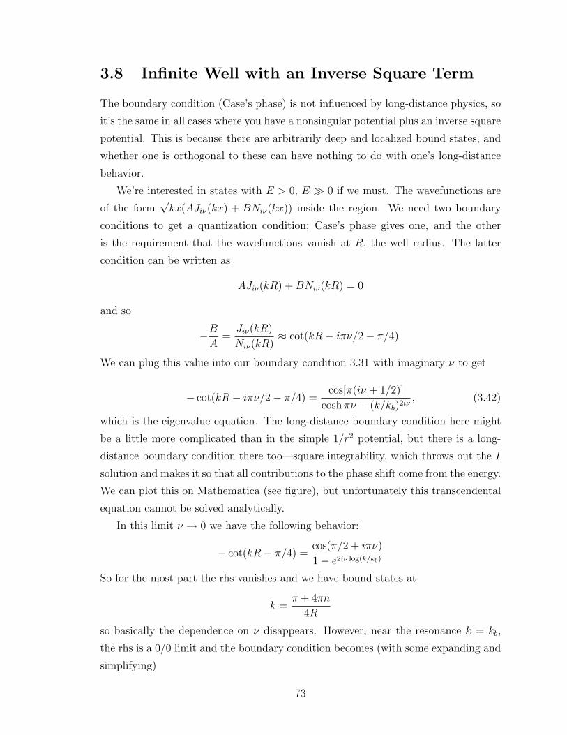
3.8 Infinite Well with an Inverse Square Term
The boundary condition (Case’s phase) is not influenced by long-distance physics, so
it’s the same in all cases where you have a nonsingular potential plus an inverse square
potential. This is because there are arbitrarily deep and localized bound states, and
whether one is orthogonal to these can have nothing to do with one’s long-distance
behavior.
We’re interested in states with E > 0, E 0 if we must. The wavefunctions are
of the form√kx(AJiν(kx) + BNiν(kx)) inside the region. We need two boundary
conditions to get a quantization condition; Case’s phase gives one, and the other
is the requirement that the wavefunctions vanish at R, the well radius. The latter
condition can be written as
AJiν(kR) +BNiν(kR) = 0
and so
−BA
=Jiν(kR)
Niν(kR)≈ cot(kR− iπν/2− π/4).
We can plug this value into our boundary condition 3.31 with imaginary ν to get
− cot(kR− iπν/2− π/4) =cos[π(iν + 1/2)]
cosh πν − (k/kb)2iν, (3.42)
which is the eigenvalue equation. The long-distance boundary condition here might
be a little more complicated than in the simple 1/r2 potential, but there is a long-
distance boundary condition there too—square integrability, which throws out the I
solution and makes it so that all contributions to the phase shift come from the energy.
We can plot this on Mathematica (see figure), but unfortunately this transcendental
equation cannot be solved analytically.
In this limit ν → 0 we have the following behavior:
− cot(kR− π/4) =cos(π/2 + iπν)
1− e2iν log(k/kb)
So for the most part the rhs vanishes and we have bound states at
k =π + 4πn
4R
so basically the dependence on ν disappears. However, near the resonance k = kb,
the rhs is a 0/0 limit and the boundary condition becomes (with some expanding and
simplifying)
73
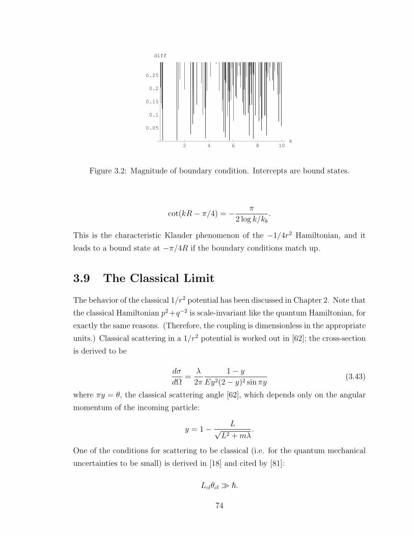
2 4 6 8 10k
0.05
0.1
0.15
0.2
0.25
diff
crapp.nb 1
Figure 3.2: Magnitude of boundary condition. Intercepts are bound states.
cot(kR− π/4) = − π
2 log k/kb.
This is the characteristic Klauder phenomenon of the −1/4r2 Hamiltonian, and it
leads to a bound state at −π/4R if the boundary conditions match up.
3.9 The Classical Limit
The behavior of the classical 1/r2 potential has been discussed in Chapter 2. Note that
the classical Hamiltonian p2+q−2 is scale-invariant like the quantum Hamiltonian, for
exactly the same reasons. (Therefore, the coupling is dimensionless in the appropriate
units.) Classical scattering in a 1/r2 potential is worked out in [62]; the cross-section
is derived to be
dσ
dΩ=
λ
2π
1− y
Ey2(2− y)2 sin πy(3.43)
where πy = θ, the classical scattering angle [62], which depends only on the angular
momentum of the incoming particle:
y = 1− L√L2 +mλ
.
One of the conditions for scattering to be classical (i.e. for the quantum mechanical
uncertainties to be small) is derived in [18] and cited by [81]:
Lclθcl ~.
74

Kayser uses this to deduce that mλ ~2—and therefore, in our units, λ 1.
Therefore, Kayser [81] argues, a classical repulsive 1/r2 potential is strongly repulsive.
(In fact, it is known [62] that the classical limit is the strong-coupling limit even
for attractive coupling.) For a sufficiently attractive potential, we’ve seen that the
classical solution is incomplete [75]: the particle collides with the center of the field
at a finite time t0 and after that the motion isn’t well-defined. However, as Zhu and
Klauder [19] point out, one can have the origin reflect everything back exactly the
way it came in, and so the scale symmetry isn’t obviously broken.
We observe that Case’s spectrum approaches continuity in the limit |Ξ| → ∞,
since the level spacing kn/km = e(n−m)/Ξ → 1 as Ξ → ∞. Consider two self-adjoint
extensions, one with a bound state at ka and another with a bound state at kb. Clearly,
for any Ξ there is an m such that kaemπ/Ξ ≤ kb ≤ kae
(m+1)π/Ξ. As Ξ →∞, therefore,
kb gets sandwiched arbitrarily closely between two wavefunctions of the extension ka,
and the self-adjoint extensions corresponding to a and b become indistinguishable.
This establishes2 that the anomaly disappears in the classical limit, which makes its
existence a little less disturbing.
There is only one “unitary” (non-dissipative) classical solution, since the phase is
irrelevant, and therefore the disappearance of phase differences is not undesired.
2Well, maybe not. k, l and λ are all large in the classical limit. However, as long as k doesn’t
grow exponentially faster than λ we’re safe.
75
Chapter 4
Global Renormalization
Now that all the expressions, and the naive formal solution, have been presented, let
us consider more physical approaches to the strongly attractive potential. There are
three questions involved: (1) do we really need self-adjointness? (2) is the coupling
constant determined by long-distance physics? (3) how many bound states should
the system have? This determines the different choices of regularization scheme, and
the different spectra, deduced by Refs. [45], [30], [86], and [22]. In this chapter, I’ll
merely introduce the schemes; their physical implications will be discussed in later
chapters.
4.1 Hardcore Cutoff
This method is due to [52] and is followed by [45] and [46]. One replaces the potential
at a short distance a with an infinite repulsive barrier. This forces the wavefunction
to vanish at that point, so that
KiΞ(ka) = 0.
Now there are two regimes of KiΞ(x), the small x regime where it oscillates wildly,
and the big x regime where it is a decaying exponential with no roots. It has a largest
zero at some xn. By making k sufficiently large we can cram all the small x behavior
into (0, a) and set a = k/xn, so the function vanishes as we require it to, and looks
like a ground state. As it happens, xn is still a “small argument,” and we can say to
good accuracy that the expression
KiΞ(ka) ∼ sin
[Ξ log
(ka
2
)− arg[Γ(1 + iΞ)]
]76
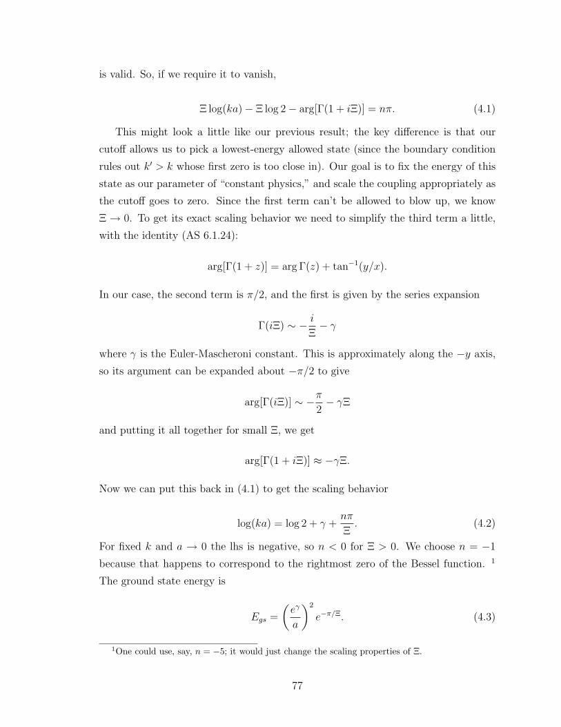
is valid. So, if we require it to vanish,
Ξ log(ka)− Ξ log 2− arg[Γ(1 + iΞ)] = nπ. (4.1)
This might look a little like our previous result; the key difference is that our
cutoff allows us to pick a lowest-energy allowed state (since the boundary condition
rules out k′ > k whose first zero is too close in). Our goal is to fix the energy of this
state as our parameter of “constant physics,” and scale the coupling appropriately as
the cutoff goes to zero. Since the first term can’t be allowed to blow up, we know
Ξ → 0. To get its exact scaling behavior we need to simplify the third term a little,
with the identity (AS 6.1.24):
arg[Γ(1 + z)] = arg Γ(z) + tan−1(y/x).
In our case, the second term is π/2, and the first is given by the series expansion
Γ(iΞ) ∼ − i
Ξ− γ
where γ is the Euler-Mascheroni constant. This is approximately along the −y axis,
so its argument can be expanded about −π/2 to give
arg[Γ(iΞ)] ∼ −π2− γΞ
and putting it all together for small Ξ, we get
arg[Γ(1 + iΞ)] ≈ −γΞ.
Now we can put this back in (4.1) to get the scaling behavior
log(ka) = log 2 + γ +nπ
Ξ. (4.2)
For fixed k and a → 0 the lhs is negative, so n < 0 for Ξ > 0. We choose n = −1
because that happens to correspond to the rightmost zero of the Bessel function. 1
The ground state energy is
Egs =
(eγ
a
)2
e−π/Ξ. (4.3)
1One could use, say, n = −5; it would just change the scaling properties of Ξ.
77
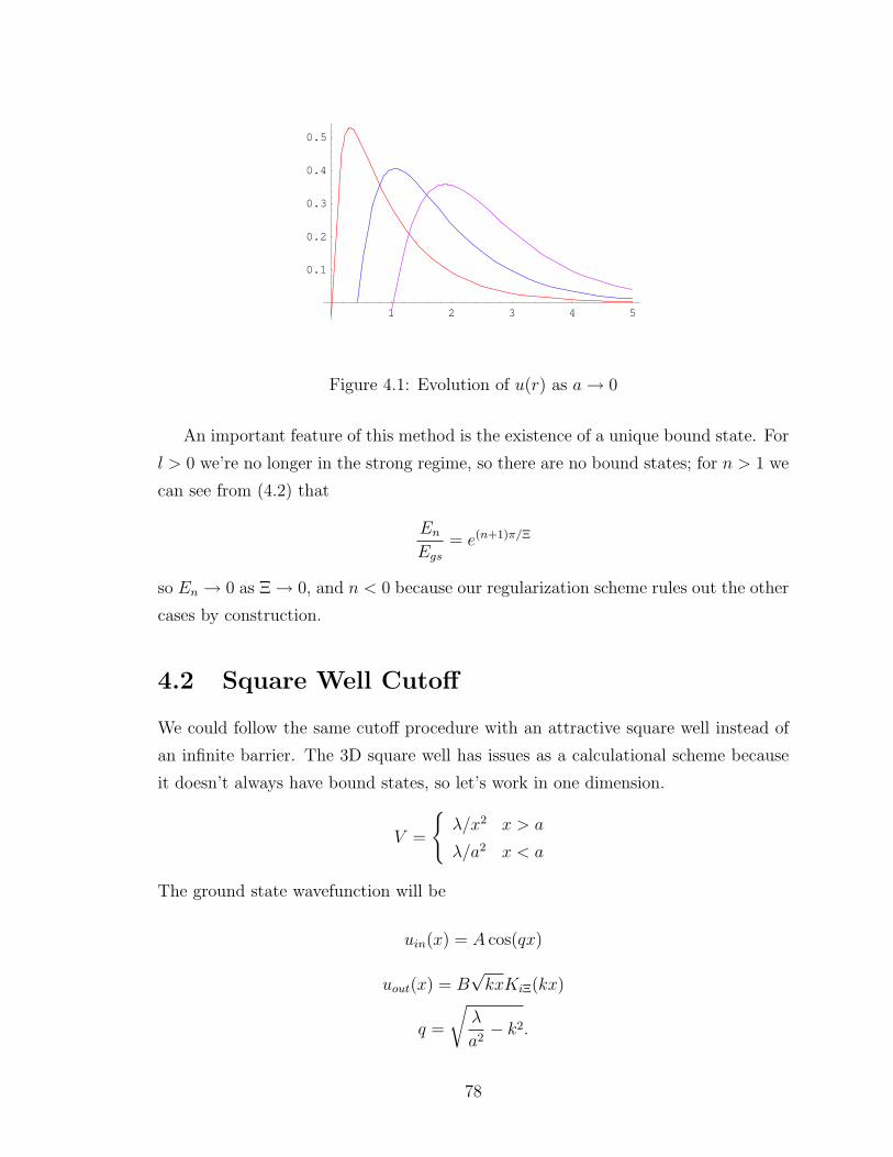
1 2 3 4 5
0.1
0.2
0.3
0.4
0.5
Untitled-1 1
Figure 4.1: Evolution of u(r) as a→ 0
An important feature of this method is the existence of a unique bound state. For
l > 0 we’re no longer in the strong regime, so there are no bound states; for n > 1 we
can see from (4.2) that
EnEgs
= e(n+1)π/Ξ
so En → 0 as Ξ → 0, and n < 0 because our regularization scheme rules out the other
cases by construction.
4.2 Square Well Cutoff
We could follow the same cutoff procedure with an attractive square well instead of
an infinite barrier. The 3D square well has issues as a calculational scheme because
it doesn’t always have bound states, so let’s work in one dimension.
V =
λ/x2 x > a
λ/a2 x < a
The ground state wavefunction will be
uin(x) = A cos(qx)
uout(x) = B√kxKiΞ(kx)
q =
√λ
a2− k2.
78
If we choose to work in the small-coupling regime, we can use the usual asymptotic
form for uout near the origin:
uout ∼ B√kx sin(Ξ log(kx) + δ).
Matching wavefunctions and their derivatives at a, we get
−qa tan(qa) =1
2+ Ξ cot(Ξ log(ka) + δ). (4.4)
Dropping all terms in (ka)2 and rearranging,
−λ− 1
2
Ξ= cot(Ξ log(ka) + δ). (4.5)
In the Ξ → 0 limit, λ→ 1/4 and the LHS blows up, so
Ξ log(ka) = nπ + δ (4.6)
as we had earlier, and we can follow through with the same logic. We will always
have a ground state this way too, since the regularized theory always has one, and
4.6 forces all the excited states to zero.
4.3 Dimensional Regularization
In [48], Camblong renormalizes the inverse square potential by means of dimensional
regularization (DR), a popular method in QFT. The idea behind DR is that problems
are sometimes better-behaved in complex dimensions, and their bad behavior shows
up as a pole at d = 3, which we can renormalize away. So instead of a cutoff, we
scale the coupling against ε, if our regularized theory lives in d± ε dimensions. This
procedure involves a lot of machinery that we don’t need for anything else, so I’ll
leave out the details; however, the point of the technique is to continue the potential
analytically in a way that does not leave it scale invariant. In our case, this means
making it a 1/r2−ε potential in 3 − ε dimensions. This is equivalent to the next—
conceptually simpler—method we consider.
4.4 Schwartz’s Way
In his 1977 paper, Schwartz [86] solved potentials of the class
79
V =λ
r2
(r
r0
)ε.
These are not exactly solvable in general, but there’s a trick for small ε. It has been
well-known for centuries [89] that negative power-law potentials have dual positive
power-law potentials, with the remarkable property that equations of motion for one
are equivalent to those for the other under a change of variable. For example, the
Kepler and harmonic oscillator problems are equivalent under the change of variables
rkep = r2sho.
This result was first discovered by Newton. Generally, as [48], [90], and [89] show,
dual power-law potentials obey the relation
(N + 2)(N ′ + 2) = 4
which is a 1-1 correspondence between (−2, 0) and (0,∞). This correspondence
carries over into quantum mechanics. The important consequence, for us, is that
N → −2 is dual to N ′ →∞, which looks like an infinite square well. We can use this
duality to solve almost singular potentials; however, let’s first look at the square well
as a limit of rn potentials.
Particle in a Box, Revisited
Consider the potential
V (r) =λ
r20
(r
r0
)n(4.7)
where λ is dimensionless, and n very large. We know there are basically two regimes:
one with r r0, where V is essentially zero; and one with r > r0, where V E. Inside, our solution is the free particle wavefunction for a particle of angular
momentum l:
uin(r) = A√krJl+1/2(kr) (4.8)
whereas outside the “well” it’s the zero-energy solution to the potential since E V
(we needn’t worry about l since the centrifugal term is negligible outside the well).
For normalizability we choose the exponentially decaying solution (let p = n+ 2):
80
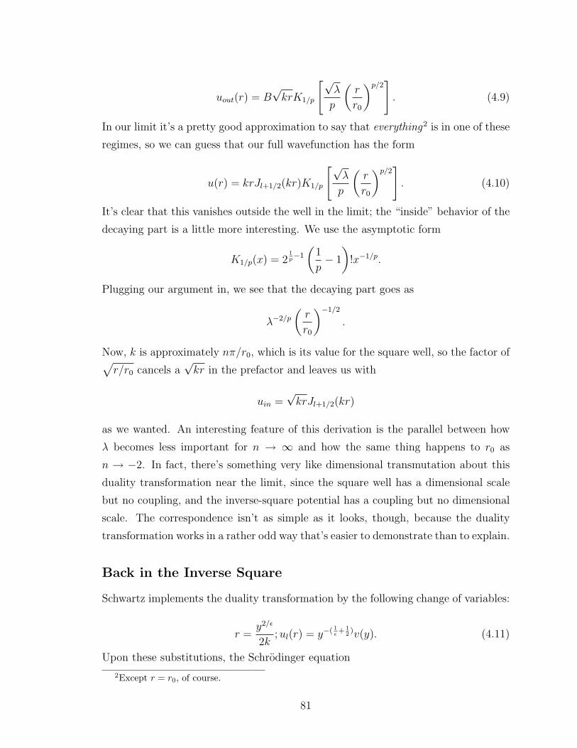
uout(r) = B√krK1/p
[√λ
p
(r
r0
)p/2]. (4.9)
In our limit it’s a pretty good approximation to say that everything2 is in one of these
regimes, so we can guess that our full wavefunction has the form
u(r) = krJl+1/2(kr)K1/p
[√λ
p
(r
r0
)p/2]. (4.10)
It’s clear that this vanishes outside the well in the limit; the “inside” behavior of the
decaying part is a little more interesting. We use the asymptotic form
K1/p(x) = 21p−1
(1
p− 1
)!x−1/p.
Plugging our argument in, we see that the decaying part goes as
λ−2/p
(r
r0
)−1/2
.
Now, k is approximately nπ/r0, which is its value for the square well, so the factor of√r/r0 cancels a
√kr in the prefactor and leaves us with
uin =√krJl+1/2(kr)
as we wanted. An interesting feature of this derivation is the parallel between how
λ becomes less important for n → ∞ and how the same thing happens to r0 as
n → −2. In fact, there’s something very like dimensional transmutation about this
duality transformation near the limit, since the square well has a dimensional scale
but no coupling, and the inverse-square potential has a coupling but no dimensional
scale. The correspondence isn’t as simple as it looks, though, because the duality
transformation works in a rather odd way that’s easier to demonstrate than to explain.
Back in the Inverse Square
Schwartz implements the duality transformation by the following change of variables:
r =y2/ε
2k;ul(r) = y−( 1
ε+ 1
2)v(y). (4.11)
Upon these substitutions, the Schrodinger equation
2Except r = r0, of course.
81

−d2u
dr2+l(l + 1)
r2u− λ
r2
(r
r0
)εu = −k2u
becomes [− d2
dy2+
[(2l + 1)/ε]2 − 14
y2+y4/(ε−2)
ε2
]v = Λv (4.12)
where
Λ =4λ
ε2(2kr0)
−ε
(The details of this procedure are worked out in Appendix A.) For sufficiently small ε,
this is basically the Schrodinger equation for a state of very high angular momentum
in a square well. Therefore, the appropriate solution is of the form
v(y) =
√√ΛyJν(
√Λy) (4.13)
for y < 1, where
ν ≈ 2l + 1
ε
and by (4.10) otherwise. We can match the functions and their derivatives at y = 1;
this is done in [48], but it turns out that we get essentially the same result if we
just require v(1) = 0, which happens if Jν(√
Λ) = 0. Schwartz quotes the following
formula for Bessel functions of very large order:
Zn = ν + Cnν1/3
where Zn is the nth zero, and Cn is basically independent of ν. So if we require that
√Λ = ν + Cnν
1/3 (4.14)
and write everything out in terms of the original variables, we see that√4λ
ε2(2r0k)−ε =
2l + 1
ε+ Cn
(2l + 1
ε
)1/3
. (4.15)
This can be rearranged in the form
log(2kr0) = −2
εlog
[2l + 1
2√λ
+Cnε
2/3(2l + 1)1/3
2√λ
](4.16)
82

where the second term in the argument of the logarithm is small relative to the first,
and can be expanded to first order using log(1 + x) ∼ x to give us
log(2kr0) = −2
ε
[log
(l + 1/2√
λ
)+
Cnε2/3
(2l + 1)2/3
]. (4.17)
Exponentiating this gives us Schwartz’s final form
En = − 1
4r20
exp
[2
εlog
λ
(l + 1/2)2
]exp
[− 4Cnε1/3(2l + 1)2/3
]. (4.18)
In particular, for l = 0 states this is
En = − 1
4r20
(4λ)2/ε e4Cn/ε1/3
. (4.19)
What our energy states look like in the limit depends on whether λ > 1/4; if so, all
the energies go to −∞, otherwise they all go to zero. We could regularize this scheme
by fixing En and scaling λ with ε, just as in our two previous schemes, and it works
in essentially the same way. The strangest consequence, though, is that
EnEm
= exp
[−4(Cn − Cm)
ε1/3
](4.20)
which always blows up. The Cn increase with n, so any higher-level energy state
vanishes relative to the ground state as ε → 0. What’s strange about this result
is that it is independent of the coupling. This means that the bare, unregularized
limit of this theory looks very different from what we derived in chapter 3 from the
Schrodinger equation—there is neither a continuum of states nor a tower.
As Schwartz’s approach and dimensional regularization turn out to be inconsistent
with those we consider next, we should point out some of the reasons they might be
inappropriate. First, there’s no reason to suppose that the limit is unique, since we
have an essential singularity in ε. In fact, we have good reason to believe it isn’t, since
things don’t look the same at all for r2+ε potentials. Suppose 4.20 held for complex
ε; we would have wildly oscillatory behavior rather than what we see.
Another way to think about it is as follows. All the bound states associated with
the Schwartz family—which all have finite numbers of nodes by construction—go
down to −∞, but a new family of bound states, each with infinitely many nodes
and finite energies, appears at the transition. (These are shallower than the previous
states, so their appearance isn’t too mysterious.) The former statement follows from
the fact that
83
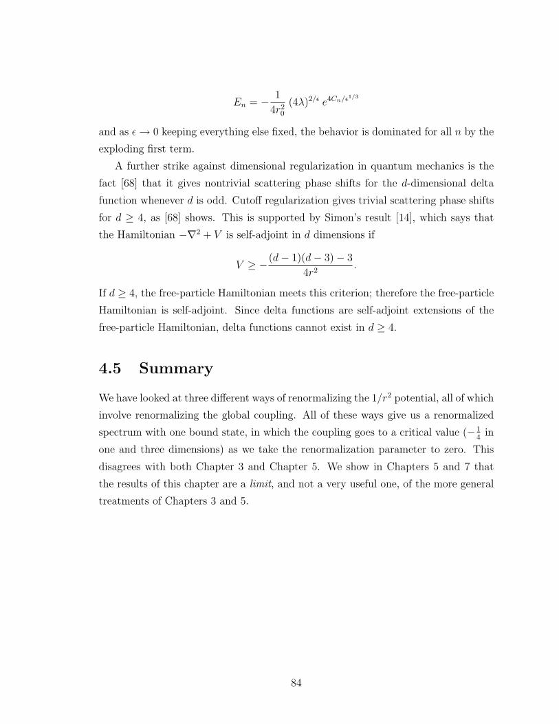
En = − 1
4r20
(4λ)2/ε e4Cn/ε1/3
and as ε→ 0 keeping everything else fixed, the behavior is dominated for all n by the
exploding first term.
A further strike against dimensional regularization in quantum mechanics is the
fact [68] that it gives nontrivial scattering phase shifts for the d-dimensional delta
function whenever d is odd. Cutoff regularization gives trivial scattering phase shifts
for d ≥ 4, as [68] shows. This is supported by Simon’s result [14], which says that
the Hamiltonian −∇2 + V is self-adjoint in d dimensions if
V ≥ −(d− 1)(d− 3)− 3
4r2.
If d ≥ 4, the free-particle Hamiltonian meets this criterion; therefore the free-particle
Hamiltonian is self-adjoint. Since delta functions are self-adjoint extensions of the
free-particle Hamiltonian, delta functions cannot exist in d ≥ 4.
4.5 Summary
We have looked at three different ways of renormalizing the 1/r2 potential, all of which
involve renormalizing the global coupling. All of these ways give us a renormalized
spectrum with one bound state, in which the coupling goes to a critical value (−14
in
one and three dimensions) as we take the renormalization parameter to zero. This
disagrees with both Chapter 3 and Chapter 5. We show in Chapters 5 and 7 that
the results of this chapter are a limit, and not a very useful one, of the more general
treatments of Chapters 3 and 5.
84

Chapter 5
Limit Cycles
A feature common to the methods we looked at in Chapter 4 is that they all involve
renormalizing the coupling. This might go against our original conception of renor-
malization as modifying only short-distance behavior, since the coupling also affects
the long-distance behavior of our theory. For instance, we saw in Chapter 3 that the
potential had many shallow bound states; even if bound states are not treated as
observables, the scattering poles associated with them certainly count as low-energy
observables. But if the coupling is fixed, what parameter are we to trade in for our
energy? A scheme to do this was implemented in Ref. [30], and later by Refs. [31],
[36], and [32]. The technique was first laid out by Lepage in Ref. [33] in a more
general context.
5.1 Running Square Well
We regularize with the following potential:
Va = − λ
r2θ(r − a)− ρ
a2θ(a− r) (5.1)
The important difference between this scheme and that in Section 4.2 is that ρ is
variable, so that the potential is discontinuous at r = a. (This is just a finite dis-
continuity, though, and we see its like in the finite well every day.) The parameter ρ
gives us something to trade in for our “energy,” and has the advantage of describing
exclusively short-distance interactions. Now our question becomes how to alter ρ as
a→ 0 to keep the “physics” fixed. But what is the physics?
Before we answer this, let’s generate a renormalization group flow for this scheme.
85
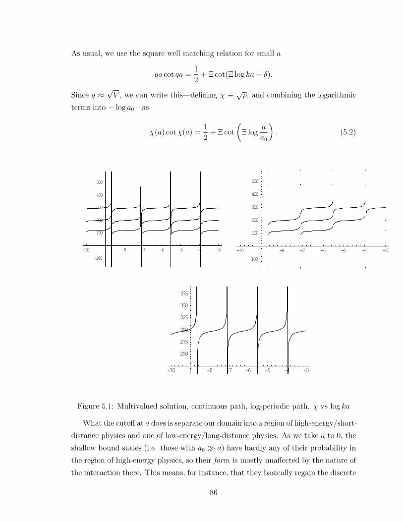
As usual, we use the square well matching relation for small a
qa cot qa =1
2+ Ξ cot(Ξ log ka+ δ).
Since q ≈√V , we can write this—defining χ ≡ √
ρ, and combining the logarithmic
terms into − log a0—as
χ(a) cotχ(a) =1
2+ Ξ cot
(Ξ log
a
a0
). (5.2)
-10 -8 -7 -6 -5 -4 -3
-100
100
200
300
400
500
-10 -8 -7 -6 -5 -4 -3
-100
100
200
300
400
500
-10 -8 -7 -6 -5 -4 -3
250
275
300
325
350
375
Figure 5.1: Multivalued solution, continuous path, log-periodic path. χ vs log ka
What the cutoff at a does is separate our domain into a region of high-energy/short-
distance physics and one of low-energy/long-distance physics. As we take a to 0, the
shallow bound states (i.e. those with a0 a) have hardly any of their probability in
the region of high-energy physics, so their form is mostly unaffected by the nature of
the interaction there. This means, for instance, that they basically regain the discrete
86
scale symmetry. Of course, if we kept χ fixed as a→ 0, a0 (and therefore the bound
state energy) would have to scale with a for the boundary conditions to match, so
the lines would cease to represent constant physics.
The situation is different with deep bound states (a0 < a), since much of their
probability is in the high-energy region, and they are affected by the details of high-
energy behavior. The flip side is that their wavefunctions are so localized that we need
very high resolution to observe them—i.e. we need to scatter high-energy states off the
potential, by E = hν. Therefore these bound states are not low-energy observables,
and we need not require them to be invariant under renormalization.
The most intuitive paths through the RG flow are given by the continuous lines
in the figure, which one gets by picking a bound state, fixing it, and changing χ
continuously and monotonically. χ decreases as a → 0—i.e. becomes weaker and
then repulsive. A heuristic way to understand what’s happening is as follows: let’s
think of the state index as the number of nodes in the the wavefunction, as we do
in nonsingular cases. (Since our theory is regularized, this is finite to start with.)
As we move a closer in, the inverse-square sector of our wavefunction gains wiggles
rapidly, and so the high-energy sector must lose them correspondingly, which it does
by increasing the potential. Even if the inside were a hard core, as we’ve seen in
Section 4.1, the wavefunction would have arbitrarily many wiggles as a got smaller—
and after that we would have no way to keep the state index. There is, therefore,
a minimal length ε down to which our effective theory is valid for a given a0. If we
had higher resolution, we could pick a lower a0—i.e. a deeper bound state—to treat
as a low-energy observable, so this isn’t necessarily a strike against the procedure.
However, if we want a procedure that gives us bound states all the way down, we
must use the so-called limit cycle (Fig 5.1).
This scheme is based on the fact that the regularized potential has infinitely many
shallow bound states with a discrete scaling symmetry. (The infinitely many shallow
bound states exist because of the slow falloff of the potential.) In the asymptotic
region, fixing any bound state to be at a certain energy gives you the same self-
adjoint extension and the same physics. (This corresponds to the picture of Chapter
3, where none of the wavefunctions has an index because they’re all at ∞.) The
log-periodic path exploits this fact by jumping discontinuously from fixing one bound
state to fixing the one just deeper than it every time the wavefunction grows another
node in the low-energy region.
87
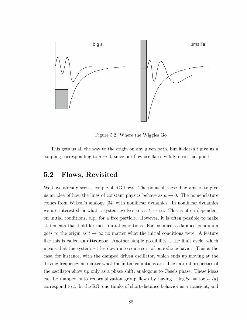
big a small a
Figure 5.2: Where the Wiggles Go
This gets us all the way to the origin on any given path, but it doesn’t give us a
coupling corresponding to a→ 0, since our flow oscillates wildly near that point.
5.2 Flows, Revisited
We have already seen a couple of RG flows. The point of these diagrams is to give
us an idea of how the lines of constant physics behave as a → 0. The nomenclature
comes from Wilson’s analogy [34] with nonlinear dynamics. In nonlinear dynamics
we are interested in what a system evolves to as t → ∞. This is often dependent
on initial conditions, e.g. for a free particle. However, it is often possible to make
statements that hold for most initial conditions. For instance, a damped pendulum
goes to the origin as t → ∞ no matter what the initial conditions were. A feature
like this is called an attractor. Another simple possibility is the limit cycle, which
means that the system settles down into some sort of periodic behavior. This is the
case, for instance, with the damped driven oscillator, which ends up moving at the
driving frequency no matter what the initial conditions are. The natural properties of
the oscillator show up only as a phase shift, analogous to Case’s phase. These ideas
can be mapped onto renormalization group flows by having − log ka = log(a0/a)
correspond to t. In the RG, one thinks of short-distance behavior as a transient, and
88
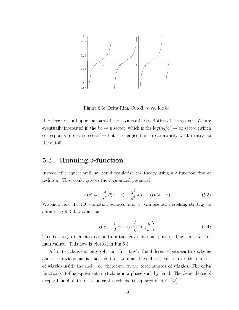
1 2 3 4 5
-10
-7.5
-5
-2.5
2.5
5
7.5
10
rg flow beane.nb 1
Figure 5.3: Delta Ring Cutoff, χ vs. log ka
therefore not an important part of the asymptotic description of the system. We are
eventually interested in the ka→ 0 sector, which is the log(a0/a) →∞ sector (which
corresponds to t→∞ sector)—that is, energies that are arbitrarily weak relative to
the cutoff.
5.3 Running δ-function
Instead of a square well, we could regularize the theory using a δ-function ring at
radius a. This would give us the regularized potential
V (r) = − λ
r2θ(r − a)− χ2
a2δ(r − a) θ(a− r) (5.3)
We know how the 1D δ-function behaves, and we can use our matching strategy to
obtain the RG flow equation:
χ(a) =1
2− Ξ cot
(Ξ log
a
a0
)(5.4)
This is a very different equation from that governing our previous flow, since χ isn’t
multivalued. This flow is plotted in Fig 5.3.
A limit cycle is our only solution. Intuitively the difference between this scheme
and the previous one is that this time we don’t have direct control over the number
of wiggles inside the shell—or, therefore, on the total number of wiggles. The delta
function cutoff is equivalent to sticking in a phase shift by hand. The dependence of
deeper bound states on a under this scheme is explored in Ref. [32].
89
Renormalization theory is interested with properties that are independent of the
cutoff potential chosen; this makes the limit cycle a more appealing solution. (It might
seem glib to infer universality from multiplicity, but limit cycle behavior is related
to the discrete scale symmetry of the spectra.) Still, the difference is not terribly
important in any particular case because both states produce the same asymptotic
spectra.
5.4 The 1/r4 Potential
This was worked out in [36]. Most of our observations still hold; an important differ-
ence is that the zero energy wavefunction is
ψ(0; r) ∼ r sin
(λ
r
).
(Let’s ignore the phase for a moment.) This oscillates rapidly at the origin, as we
have learned to expect, but in the infrared regime it has no nodes for r > λ/π—as
opposed to the 1/r2 potential, which has infinitely many nodes both ways. So if you
impose an ultraviolet cutoff, ψ(0; r) has only finitely many nodes, and—since it is the
shallowest bound state—ψ(−E; r) has as many or fewer. Therefore, the regularized
solution has only finitely many bound states, and the continuous path preserves the
number of bound states.
As before, we can regulate the potential with a square well cutoff or a ring cutoff.
The procedure is a little harder than before because we lack usable analytic expres-
sions for anything but the zero energy solution. However, the state we are fixing is a
shallow state, so for a short-distance cutoff it’s reasonable to take |E| |V | and use
the zero energy outside solution. With this, our wavefunction is
ψ(0; r) =
A sin qr r < a
Br cos(λr
+ φ)
r > a(5.5)
φ is a phase shift between the cosine and sine exterior solutions. The boundary
condition one gets by imposing continuity at r = a is
q cot qa =1
a+λ
a2tan
(λ
a+ φ
),
which we can rewrite as
90
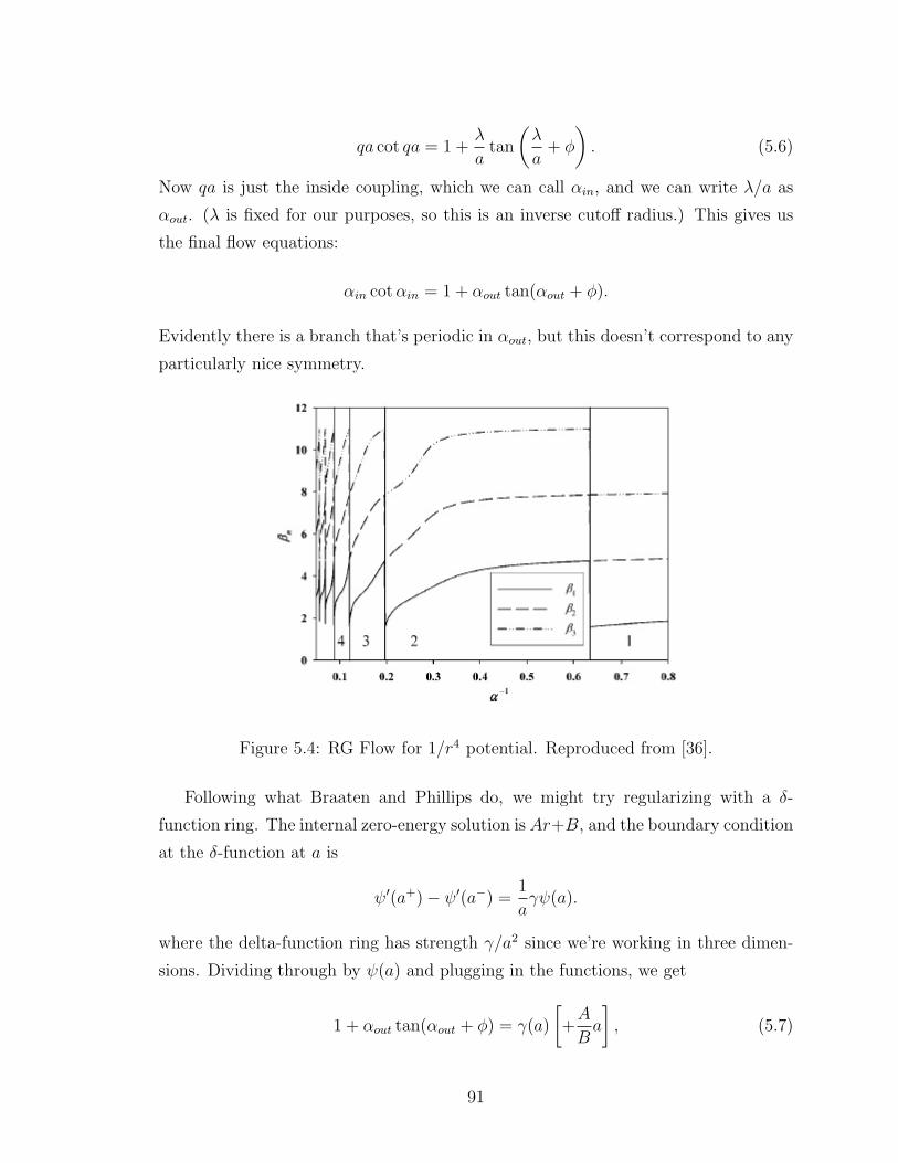
qa cot qa = 1 +λ
atan
(λ
a+ φ
). (5.6)
Now qa is just the inside coupling, which we can call αin, and we can write λ/a as
αout. (λ is fixed for our purposes, so this is an inverse cutoff radius.) This gives us
the final flow equations:
αin cotαin = 1 + αout tan(αout + φ).
Evidently there is a branch that’s periodic in αout, but this doesn’t correspond to any
particularly nice symmetry.
Figure 5.4: RG Flow for 1/r4 potential. Reproduced from [36].
Following what Braaten and Phillips do, we might try regularizing with a δ-
function ring. The internal zero-energy solution is Ar+B, and the boundary condition
at the δ-function at a is
ψ′(a+)− ψ′(a−) =1
aγψ(a).
where the delta-function ring has strength γ/a2 since we’re working in three dimen-
sions. Dividing through by ψ(a) and plugging in the functions, we get
1 + αout tan(αout + φ) = γ(a)
[+A
Ba
], (5.7)
91
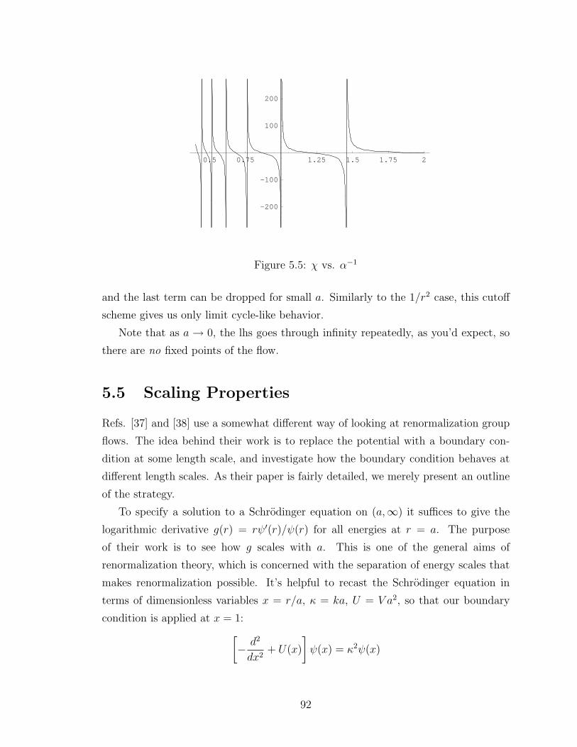
0.5 0.75 1.25 1.5 1.75 2
-200
-100
100
200
rg flow beane.nb 1
Figure 5.5: χ vs. α−1
and the last term can be dropped for small a. Similarly to the 1/r2 case, this cutoff
scheme gives us only limit cycle-like behavior.
Note that as a → 0, the lhs goes through infinity repeatedly, as you’d expect, so
there are no fixed points of the flow.
5.5 Scaling Properties
Refs. [37] and [38] use a somewhat different way of looking at renormalization group
flows. The idea behind their work is to replace the potential with a boundary con-
dition at some length scale, and investigate how the boundary condition behaves at
different length scales. As their paper is fairly detailed, we merely present an outline
of the strategy.
To specify a solution to a Schrodinger equation on (a,∞) it suffices to give the
logarithmic derivative g(r) = rψ′(r)/ψ(r) for all energies at r = a. The purpose
of their work is to see how g scales with a. This is one of the general aims of
renormalization theory, which is concerned with the separation of energy scales that
makes renormalization possible. It’s helpful to recast the Schrodinger equation in
terms of dimensionless variables x = r/a, κ = ka, U = V a2, so that our boundary
condition is applied at x = 1:[− d2
dx2+ U(x)
]ψ(x) = κ2ψ(x)
92

xψ′(x)
ψ(x)
∣∣∣∣x=1
= g(1, κ)
(We use a slightly nonstandard form of the logarithmic derivative in order to make
g dimensionless.) Of course, we could impose the boundary condition at any other
value of x, say x = λ. It would be useful to have the new equation be as close to
the form of the old ones for comparison, so we might want to express the boundary
condition as x/λ = 1. What we really want to do is rescale the Schrodinger equation
so that the boundary condition is of the form x = 1 (we will see the benefit of this
when we are done); this is done by dilating the Schrodinger equation, as we did in ch.
1, but since we are not necessarily working with scale invariant potentials we have to
be careful. The first step is to dilate the wavefunction:
ψλ(x) = ψ(λx)
So when you differentiate it with respect to x a factor of λ pops out, and for the
Schrodinger equation to retain its form the potential must scale appropriately, so
that
Uλ(x) = λ2U(λx)
and
κλ = λ2κ.
The boundary condition scales as it should:
gλ(x, κλ) = g(λx, κ).
In terms of these variables our scaled equations look like our original equations:[− d2
dx2+ Uλ(x)
]ψλ(x) = κ2
λψλ(x)
xψ′λ(x)
ψλ(x)
∣∣∣∣x=1
= gλ(1, κλ)
We can write formal expressions for how Uλ and gλ depend on λ. We are interested
in two cases, the λ → 0 limit, which corresponds to probing the system at short
distances and is related to our cutoff schemes, and the λ → ∞ limit, since that
corresponds to asymptotic low-energy properties.1 It’s possible to get a fair amount
1Mueller and Ho [37] are interested mostly in the λ→∞ properties.
93
of information out of the problem from the form of Uλ. For a potential that falls
off slower than 1/r2, Uλ tends to become very large as λ → ∞, and for one that
falls off faster it tends to vanish. Scale invariant potentials don’t do anything at all.
This is linked to the fact that some potentials are more “active” in some regimes; for
instance, the 1/r potential has infinitely many shallow bound states, while the 1/r4
potential has infinitely many deep bound states.
The relation for the boundary condition is derived from the following form of the
Schrodinger equation in terms of logarithmic derivatives:
x∂g
∂x= x2(U(x)− E) + g(x)− g(x)2
If we plug in all the scaling factors and do out the algebra, the scaled version of this
is
λ∂λgλ(x, κλ) = x2(Uλ(x)− Eλ) + gλ(x, κλ)− g2λ(x, κλ) (5.8)
We are not interested in the dependence of gλ on x, since we only ever evaluate it at
x = 1, so we can write it as gλ(κλ), and expand out in powers of κ. We are most
interested in low-energy solutions, so we can drop all powers of κ and investigate
leading behavior. (At least, it’s worth a try.) For the case of the inverse-square
potential, since U doesn’t flow, we find that the equation is
C + g − g2 = 0. (5.9)
For C > −1/4, this equation has two real roots; otherwise, it has complex roots, which
do not correspond to a self-adjoint boundary condition. (For more on this, see ch. 6.)
This shows that there isn’t a single asymptotic solution for the boundary condition.
These properties are the same at both the infrared and ultraviolet ends, which is
expected since the 1/r2 potential done by the method of self-adjoint extensions has
an exact limit cycle at all levels.
The scaling method also gives us a pleasing duality between the behavior of long-
range forces like 1/r in the infrared and shorter-range forces like 1/r4 in the ultraviolet.
(We are thinking of the attractive behavior; the repulsive potentials always have a
fixed point at the Friedrichs extension.) The fixed point, as λ → 0 or λ → ∞, is
U → −∞ in this case. Ref. [37] works out the infrared case; we do the ultraviolet,
which is more relevant to our purposes. By construction of our boundary condition,
x = 1 always, so for a low energy state,
94
λ∂λgλ = −U(1)1
λm+ gλ − g2
λ (5.10)
where m = −n + 2 for an xn potential. Since the only dependence is on λ, we can
rewrite the partial derivatives as total derivatives, and consider
λdg
dλ− g + g2 = − a2
λm
which can be solved in terms of Bessel functions of argument 1/xm/2. For the partic-
ular case of the 1/r4 potential, Mathematica yields
g(λ) =(−λ+ aA) cos
(aλ
)− (a+ Aλ) sin
(aλ
)λ[cos(aλ
)+ A sin
(aλ
)]Asymptotically this is
g(λ) ∼ a
λ
A cos(aλ
)− sin
(aλ
)cos(aλ
)+ A sin
(aλ
) .The form of boundary condition that we’ve used earlier is λg(λ), so this is consistent.
The condition is periodic in 1/λ, as we found by our previous methods. One can
escape the periodicity only by allowing λ to take on complex values in order to turn
the trig functions into hyperbolic functions. Doing this corresponds to the complex
boundary conditions that we discuss in the next chapter. Interestingly, the flow
behavior of long-range potentials as λ → ∞ is very similar to this (for details, see
[37]).
The λ→∞ limit of this potential is also interesting because it actually has a fixed
point. In this case, U → 0 for the 1/r4 potential, and therefore (for the zero-energy
solution) the equation becomes:
λdg
dλ= g − g2
The solution to this is
g(λ) =λ
−C + λ
which flows to 1 as λ→∞. This is a manifestation of the fact that the potential has
no infrared pathologies because it falls off sufficiently fast. However, the short distance
physics still affects our low-energy observables, and renormalization of the ultraviolet
spectrum is still required; for example, the zero-energy phase shift is determined by
Case’s phase/a regularization scheme:
95
ψ(0, r) = Br cos
(λ
r+ φ
)and therefore the scattering length a is given by
a = λ cotφ.
The scaling technique is equivalent to the δ-function ring cutoff in the ultraviolet,
since both in effect specify the logarithmic derivative of the function at the boundary
point. The difference is one of interpretation. In one case, you squeeze the function
in and out of the r = 1 area by stretching and contracting the coordinate variable
and find out how the logarithmic derivative evolves; in the other, you counteract the
changes of the outside region by adding a term to the logarithmic derivative that’s
big enough to cancel it out.
5.6 Consistency with Chapter 4
We now have two different pictures of the 1/r2 potential—one with a single bound
state and another with infinitely many. The cutoff methods and self-adjoint extensions
both give the (asymptotic) relation
EnEm
= e2(n−m)π/Ξ.
As Ξ → 0, if we fix an arbitrarily chosen bound state Em at k, both methods agree in
sending all others with n < m to zero. However, the method of self-adjoint extensions
sends a whole family of states m < n to −∞, whereas the cutoff schemes of Ch. 4 do
not have these states at all. Don’t the deep states matter? The answer is that they
don’t, from our EFT perspective, because they are highly localized, and therefore
cannot be probed unless we have arbitrarily good resolution—in which case we know
the theory exactly at all energies and renormalization is unnecessary.
For example, one of the ways to detect a bound state is to look for poles in the
scattering length or, equivalently, in tan δ0. Levinson’s theorem (see Chapter 7 or
[62]) says that the scattering phase shift goes through Nπ as k is increased from 0
to ∞, where N is the number of bound states. (We require that it be a monotonic
function of k, which is why it goes through π instead of going back to zero.) However,
96
to detect a bound state with energy kb you need to be able to send in a beam of energy
kb, and this ensures the privacy of deep bound states.
From what we’ve seen so far it seems that RG flows asymptotically produce the
same behavior as self-adjoint extensions. This is not too surprising if you think of
self-adjoint extensions as corresponding to the possibilities for point interactions at
the origin. The renormalization techniques we have used in this chapter work by
adding smeared-out point interactions, and self-adjoint extensions are the limiting
forms as ka → 0. This would explain, for example, why the self-adjoint extensions
of the 1/r2 potential have a limit cycle going all the way down. This is also why
self-adjoint extensions are not a complete treatment of any physical problem; at some
energy level we enter the regime of transient (high-energy) physics, where the true
potential differs from its asymptotic form.
Spectra Unbounded from Below
Strongly attractive power-law potentials have very often been rejected as unphysical
because they have spectra unbounded from below. But as our treatment in this
chapter has shown, as far as the two-body self-adjoint problem is concerned the
unboundedness is not an issue, and in fact it’s impossible even to tell—except with
infinite energy resolution—whether a given potential is unbounded from below. No
doubt there are several physical situations where such a potential would be entirely
unacceptable; however, as we see in the context of the Efimov effect [27], there are
some where it gives a powerful description of the physics.
The fact that the asymptotic solution is unbounded also gives us a way of classify-
ing renormalization schemes. We saw earlier in this chapter that the continuous paths
would not go all the way down, and mentioned that this was due to unboundedness.
This connection is important, so let’s go over it more carefully. Given a regulariza-
tion scheme Σ of the λ/r2 potential, we denote the regularized potential by V (Σ, a, x)
and the lower bound (see Chapter 2) of the Hamiltonian by B(Σ, a). For |x| > a,
V (Σ, a, x) ≡ V (x) for all regularization schemes. Clearly, if V (Σ, a, x) ≤ V (Σ′, a, x)
at all x ∈ Rn, then B(Σ) ≤ B(Σ′). Therefore, for all cutoff regularization schemes,
B(Σ, a) ≤ B(Σ0, a), where Σ0 is an infinite barrier for |x| < a. Since B(Σ0, a) → −∞as a → 0 (new wiggles, and new states, keep appearing at a log-periodic rate),
B(Σ, a) → −∞ too.
Now suppose we want to fix a bound state of index j. This is the same as fixing
97
the ground state (or bounding the ground state energy from below), and is therefore
equivalent to fixing B(Σ, a) as we take a → 0. We know we can’t do this because
B(Σ, a) → −∞ as we just proved. This shows us that no regularization scheme
that keeps the long-distance physics fixed can also fix the bound state with j nodes;
thus the suggestion in [31] that the unbounded spectrum might result from using the
wrong point interaction is invalidated. For the 1/r4 potential, it shows that there is
no way to renormalize the system to arbitrary distances so that it has a fixed number
of bound states. On the other hand, it also shows that any renormalization scheme
that maintains the lower bound of the spectrum must force the coupling up to the
critical value, where it becomes a Klauder phenomenon, as discussed in Chapter 7.
This argument is harder to make rigorous for schemes like Schwartz’s, but clearly
the basic idea carries through. The bound of the regularized theory goes smoothly
to −∞, and if you fix it the only way to keep the bound is to change the theory
continuously so that in the limit you get a bounded theory. This clearly can’t still be
very singular, so one has to push it up to the critical point where the theory becomes
bounded. For the 1/r2 potential this is at λ = −14; for more singular potentials it’s
at zero coupling (the renormalized theory is a delta function).
5.7 RG Treatment of Weak Coupling
Let’s return to the non-Friedrichs extensions we discussed in chapter 3 with our new
apparatus, which allows us to talk about the extensions of the 1/r2 potential from a
more physical point of view.
5.7.1 What Sort of Physics?
A curious feature of these extensions is that a potential that appears to be everywhere
positive has states of negative energy. It has been suggested ([20],[51]) that this is
due to δ-function interactions. It is certainly true that all short-distance physics is
due to delta function-like operators from an EFT point of view; however, it turns out
not to be true that
V =λ
x2θ(x− a)− β
aθ(a− x)
produces one of these extensions as a→ 0. From our usual boundary condition
98
qa tan qa =1
2+ ka
K ′ζ+1/2(ka)
Kζ+1/2(ka)
since qa ∼√βa → 0, we can use the small-angle approximation, so that (letting
ξ ≡ (ka/2) and ν = ζ + 1/2)
βa =1
2+ ν
ξνΓ(−ν)− ξ−νΓ(ν)
ξνΓ(−ν) + ξ−νΓ(ν)(5.11)
There are two easily solved cases. The first is when ν is sufficiently big that we can
drop the xν terms; the other is when ν → 0. In the first case, the equation reduces to
0 ≈ βa =1
2− ν ⇒ ν = 1/2 ⇒ λ = 0 (5.12)
so the only solution is our old acquaintance the delta function. When ν 1 we can
use Γ(ν) ∼ 1/ν to get
0 =1
2− ν
ξν + ξ−ν
ξν − ξ−ν
and the rhs is recognizably hyperbolic:
1
2= ν coth(ν log ξ) ⇒ ν ≤ 1
2⇒ λ ≤ 0 (5.13)
and therefore the potential must be attractive for bound states to exist. This is telling
us less than we assumed, since anything in the ν ≈ 0 regime is attractive.
So what sort of attractive point potential would work? The following theorem,
due to Simon [85], is suggestive:
Theorem 8 (Simon, 1975) Given a (not wildly pathological) 1D function V (x)
such that ∫ ∞
−∞(1 + x2)|V (x)|dx <∞,
the Hamiltonian with potential λV has a bound state for small λ > 0 iff∫ ∞
−∞V dx ≤ 0,
and if the integral is zero, then the potential has a bound state for all λ > 0.
99
As it happens our inverse square potential doesn’t fit Simon’s hypotheses because
of its long-range character, but if we cut it off at a suitable R 1/k the theorem
becomes applicable. Consider the potential
V =λ
x2θ(R− x)θ(x− a)− β
a2θ(a− x)
If β > λ > 0 then this potential supports a bound state for arbitrarily large R. Of
course, the bound state energy might depend on R—though this is unlikely, since the
state is much more localized than the potential. Anyway, Simon’s theorem motivates
us to see if this potential works. We are forced to choose the weak interior coupling
regime to expand out tan qa =√β. The boundary condition permits nontrivial
results this time: β = −λ for biggish λ, and β < −λ for small λ. However, the limit
is problematic, and you can see this directly from the fact that the only dimensional
parameter in the problem is a.
So we have an irregular theory, and some kind of renormalization is called for.
What we need to do is run either β or λ against k and see if the theory can be
renormalized. Simon’s theorem might suggest that somehow one should try and keep
the integral fixed; this entails fixing a relationship between β and λ. This is a bad
idea, since one will have to force the external coupling to zero as a→ 0, and this will
give us back the delta function.2 So we run the coupling of the short-distance term
against the cutoff radius a. (For the moment let’s assume ν ≈ 0.) The flow equation
is similar to that in Beane’s case:
−χ(a) tanχ(a) =1
2− ν coth(ν log(a/a0))
where we’ve used the previous approximation. But the flow looks like this:
Unexpectedly, χ blows up at a0, which means that β blows up at a0. There are
infinitely many choices of path for smaller values of χ, but all of them flow to χ = 1/2
or some bigger χ. Using a delta function regulator forces χ to flow to 1/2. Both
solutions correspond to a counterterm of the form δ(x)/x, but it’s unclear why the
square well regularization gives you so much freedom.
Looking at the wavefunctions makes it evident that the potential is pathological
in one dimension, at least in the attractive case, since both solutions x1−ζ and xζ
vanish at the origin. For one dimensional potentials a ground state that vanishes
at the origin is abnormal, and has been conjectured [98] to imply an impenetrable
barrier at the origin.
2We’re assuming a result from Chapter 7.
100
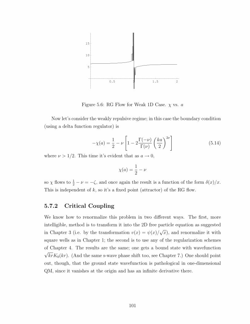
0.5 1 1.5 2
5
10
15
gweak.nb 1
Figure 5.6: RG Flow for Weak 1D Case. χ vs. a
Now let’s consider the weakly repulsive regime; in this case the boundary condition
(using a delta function regulator) is
−χ(a) =1
2− ν
[1− 2
Γ(−ν)Γ(ν)
(ka
2
)2ν]
(5.14)
where ν > 1/2. This time it’s evident that as a→ 0,
χ(a) =1
2− ν
so χ flows to 12− ν = −ζ, and once again the result is a function of the form δ(x)/x.
This is independent of k, so it’s a fixed point (attractor) of the RG flow.
5.7.2 Critical Coupling
We know how to renormalize this problem in two different ways. The first, more
intelligible, method is to transform it into the 2D free particle equation as suggested
in Chapter 3 (i.e. by the transformation v(x) = ψ(x)/√x), and renormalize it with
square wells as in Chapter 1; the second is to use any of the regularization schemes
of Chapter 4. The results are the same; one gets a bound state with wavefunction√krK0(kr). (And the same s-wave phase shift too, see Chapter 7.) One should point
out, though, that the ground state wavefunction is pathological in one-dimensional
QM, since it vanishes at the origin and has an infinite derivative there.
101
5.7.3 Two Dimensions
(Recall that in two dimensions the weak regime is for 0 ≤ λ < 1.) Suppose we try
regular 2D delta functions: the matching condition for ν 1 is
β = ν coth(ν log(ka/2)). (5.15)
If long-distance physics is fixed then β → −ν as a → 0, independent of k. (We
approximated out the Bessel function; For small ν consistency demands small β.)
Here, again, we have a fixed point in the flow, and it corresponds to an unregularized
2D delta function. Amusingly, this equation explains “why” the 2D delta function
needs to be renormalized, since ν = 0 requires β = 0 too. For less weak coupling the
expression is not as compact, but the result is pretty similar:√βJ ′0(√β)
J ′0(√β)
= −ν
5.7.4 Conclusions
In two dimensions it’s reasonably clear what’s going on. There’s a delta function
interaction at the origin that just overcomes the repulsive enveloping potential; it
flows to a fixed point under renormalization, because a finite-strength delta function
is too strong in two dimensions (see Chapter 1). The three-dimensional problem,
too, is relatively sensible; we used Meetz’s regularization scheme [6] in Chapter 3 to
argue for the Friedrichs extension. With the one dimensional repulsive case, too, one
can argue for the Friedrichs extension from the positivity of the potential. However,
as Simon’s theorem proves, a regularized 1D attractive potential does have a bound
state.
The wavefunction is pathological at the origin, but this doesn’t affect low-energy
physics. Once we know that there are (a) self-adjoint extensions and (b) reasonable
renormalization schemes, our work as physicists is done. It’s entertaining to speculate
about the “true causes” of pathologies, but a good answer isn’t necessary, which makes
one feel better about not having one.
102

Chapter 6
Fall to the Center
In the classical two-body problem, fall to the center happens if the particles collide
at a finite time. For the l 6= 0 case—which is the interesting one, classically—the
centrifugal barrier must be overcome, and a class of potentials that does this is the
attractive 1/rn, n ≥ 2 potentials. Under these potentials, the two bodies are moving
infinitely fast towards each other as they collide, so the boundary conditions for the
collision are ill-defined. If the collision is elastic, they bounce back in a way that
keeps the solution time-reversal invariant, moving with infinite velocity at first. If we
had a bound state (total E < 0) to begin with, this motion is repeated endlessly. The
total energy of the system is conserved; this corresponds to the quantum mechanical
problem as we have been doing it, in which a bound state evolves without dissipating
energy. Classically the collision might also be inelastic; the particles might stick
together after they collide. The energy has got to go somewhere, even in the classical
view, but if we aren’t interested in the details it’s easy to treat the energy as just
being dissipated. The self-adjoint operator formalism of quantum mechanics does not
permit this general sort of dissipation, however, since the (unitary) time evolution of
a state is given by ψ(t) = e−iEtψ(0) for an eigenstate, and evidently1
〈H〉ψ(t) = 〈ψ(t) |H|ψ(t)〉 = e−iEteiEt 〈ψ(0) |H|ψ(0)〉 = 〈H〉ψ(0)
and energy is conserved for eigenstates. Since any Hermitian operator has a complete
set of eigenstates, it has at least some nontrivial eigenstates (bound or not); but
in the classical picture with an inelastic collision, there simply can’t be any energy
eigenstates.
1I have used Dirac notation this once because the ideas are so familiar.
103
The quantum theory of inelastic collisions [62] deals with this problem by in-
troducing the so-called multiple-channel method, where energy and probability are
allowed to slosh back and forth among the “channels” corresponding to interactions
of the subsystems. Energy is conserved for the whole system, but not in any par-
ticular channel; therefore, projections of the Hamiltonian to a particular channel are
not necessarily self-adjoint operators. Note, however, that as the Hamiltonian is not
time-dependent, neither are its projections.2
A special case of this idea is when incoming particles are absorbed at the origin;
this leads to probability loss, as well as energy loss, from the system. Clearly, one
way to get this would be if we had complex eigenvalues of the form Ex − iEy, since
this would lead to time evolution given by
〈ψ(t)|ψ(t)〉 = e−2Eyt
and the probability of finding the particle anywhere would decay exponentially.
6.1 Contraction Semigroups
The time evolution operators U(t) ≡ eiHt form a group under composition, since
U(t)U(t′) = U(t+ t′), and each element has the inverse U(−t), which is also unitary.
Probability-dissipating operators V (t) have the same additive property, but their
inverses create probability—so the group splits into two parts, called semigroups.
The semigroup that dissipates probability is called a contraction semigroup; these
structures are common in mathematical physics, especially in the study of the heat
equation. The generator of a contraction semigroup is called a dissipative operator.
The theory of semigroups has been extensively developed, and most results are too
technical to be directly helpful; in practice one typically just assumes that complex
phase shifts work because they seem to. This is the attitude, for instance, of Schiff
[61]. The exception is the relation linking semigroups and the machinery of self-adjoint
extensions, which we will now discuss.
Recall from Chapter 2 that a densely defined Hermitian operator generates unique
unitary time evolution iff its deficiency indices are (0, 0). For deficiency indices (1, 1)
2This is the Schrodinger picture, in which wavefunctions carry the time dependence. If one were
particularly interested in energy loss one might prefer the equivalent Heisenberg picture, in which
the operators (dynamical variables) of the theory carry the time dependence.
104
we saw that the self-adjoint extensions were parameterized by U(1), a one-parameter
family of boundary conditions. One way to represent U(1) is as eiθ. One is motivated
by mindless curiosity, as usual, to ask what happens if θ is permitted to be complex.
Since |ea+ib| = ea, this is the same as asking what happens if, instead of extending
our domain by functions of the form
Ψ+ + eiθΨ−,
we allow
Ψ+ + AeiθΨ−
for some fixed A ∈ R+ (or as Ψ+ + zΨ− for z ∈ C). (This isn’t all that unreason-
able, since many of the examples of Chapter 2 make sense with complex boundary
conditions.) Now suppose we wanted to prove that our self-adjoint extension G was
in fact self-adjoint: one way to do this would be to check for complex eigenvalues of
the form c = a + ib by solving (G − c)ψ = 0, or (ψ, (G − c)ψ) = 0 for an arbitrary
ψ ∈ DG. ψ can be written as φ+ λ(Ψ+ + eiθΨ−), so that
0 = (ψ,Hψ)
= (φ,Hφ) + λ(φ,H(Ψ+ + eiθΨ−)) + λ((Ψ+ + eiθΨ−), Hφ)
+|λ|2(Ψ+ + eiθΨ−, H(Ψ+ + eiθΨ−)).
Of these the first term is the expectation value of a Hermitian operator in its domain,
so it must be real. Because φ ∈ DH , the domain of the original symmetric operator,
we can rewrite the second pair of terms as
λ(Hφ,Ψ+ + eiθΨ−) + λ(Ψ+ + eiθΨ−, Hφ).
These terms are conjugates, so their sum is real. Note that this only uses the fact
that Ψ+ and Ψ− are in the adjoint domain. Similarly, the last term can be rewritten
as
|λ|2[i− i+ ieiθ(Ψ+,Ψ−)− ie−iθ(Ψ−,Ψ+)
](6.1)
and since the last two terms are just conjugates this vanishes. Therefore,
=[(ψ, (H − c)ψ)] = =[(ψ,Hψ)] + =[(ψ,−cψ)] = =[−c(ψ, ψ)] = −b 6= 0.
105
A fortiori, (H−c)ψ 6= 0 and c is not an eigenvalue. Now suppose that ψ = φ+pΨ+ +
qΨ−, which is a more general boundary condition. The first two terms would still
cancel out, and the third term would be
|λ|2[i|p|2 − i|q|2 + ipqeiθ(Ψ+,Ψ−)− ipqe−iθ(Ψ−,Ψ+)
](6.2)
The cross terms are still conjugates and add up to give a real value, but that leaves
us with the certainly imaginary quantity
i|λ|2(|p|2 − |q|2).
For a complex eigenvalue to have any chance of working, the condition is that
|λ|2(|p|2 − |q|2) = b.
Since p and q are determined by our choice of self-adjoint extension, b is fixed by the
boundary condition, and in particular, is always going to have the same sign. This
gives us an important result:
Theorem 9 All the eigenvalues of extensions of a symmetric H are in the same
closed half-plane.
(Our discussion of this result has followed Ref. [7].) The boundary condition is
either entirely a source or entirely a sink, that is, probability is either only created
or only lost. This might seem trivial, but it isn’t; we could have had eigenvalues in
both half-planes, in which case we would have a mixture of source and sink behavior
for different states.
In the rest of our treatment we will assume that permitting complex
θ is equivalent to permitting complex numbers instead of real numbers
in our boundary conditions. These complex eigenvalues are about the furthest
meaningful generalization we can make. Suppose we try to use the whole adjoint
as our nonunitary Hamiltonian, and send in a scattering state along the half-line.
When it gets to the origin, it doesn’t know what to do because there’s no boundary
condition there, and we cease to have a well-defined problem.
6.2 Dissipative Particle on Half-Line
In Chapter 2, we had derived the boundary condition for a particle on the half-line
to be
106
ψ(0) = αψ′(0)
Let α = ia. Suppose we send in a scattering state Ae−ikx + Beikx. The boundary
condition enforces A+B = ka(A−B). For a = 0, the boundary condition is A = −B,
which is self-adjoint. (This is the Friedrichs extension.) As we increase a,
B =1− ka
1 + kaA
so the amplitude of the reflected wave diminishes until at ka = 1 it vanishes altogether.
However, as we increase k further we get back some reflection, andB/A asymptotically
approaches 1 again. The vanishing of the reflected wave for certain values of k is
familiar from wave mechanics.
One might interpret the absorptive solution as saying that there’s no outgoing
wave and the particle has been absorbed at the origin—or, more mundanely, just
transmitted through the origin. This is a good example of how complex phase shifts
work; we can replace all information about the negative half-line with a boundary
condition. It cannot be emphasized enough that using a dissipative Hamiltonian on
a subspace does not necessarily imply pathological behavior on the whole space or in
the physical problem.
The boundary condition α = ia does not permit any bound states. But letting
α = −(1−i)a gives us a normalizable eigenfunction of energy −(
1a−ai
)2, which decays
exponentially with time.
6.3 Absorption by a 1/r2 potential
The first treatment of absorption by singular potentials is by Vogt and Wannier (1954)
[8], who worked the scattering problem for 1/r4 potentials. Perelomov and Popov
(1970) [20] treated absorption by a 1/r2 potential in some detail, and Alliluev (1971)
[21] proved that the set of eigenfunctions was complete. The solution of greatest
interest corresponds to complete absorption. The interest in this solution is chiefly
due to three features: its similarity to the classical limit with absorption, its analytic
relation to the weakly attractive problem, and its connection with the experimental
realization of 1/r2 potentials by scattering neutral atoms off a charged wire [23]. In
addition to these, it is the only extension for which scale invariance holds.
107
To keep the problem as simple as possible—and also to relate it directly to
experiment—we will work in two dimensions. We saw previously how a boundary
condition can be derived from the method of self-adjoint extensions for this potential;
here we will merely cite the result:
iνψ + rψ′
iνψ − rψ′=
Γ(−iν)Γ(iν)
(kbr
2
)2iν
(6.3)
Self-adjoint extensions correspond to real choices of kb, for which the rhs has magni-
tude one; allowing kb to be complex relaxes this restriction. In particular, it allows us
to pick a sort of “Friedrichs extension,” in which the solution corresponding to J−iν
vanishes.
It’s easiest to work the scattering problem by requiring that ψ ∼ (kr)−iν near the
origin. If the form we send in is AJiν +BNiν , this means that
B
πΓ(−iν) cosh(πν) =
A
Γ(1 + iν)(6.4)
which means that
B
A=
π
Γ(−iν)Γ(1 + iν) cosh(πν). (6.5)
This can be simplified, using the reflection formula for gamma functions, to
B
A=− sin(iπν)
cos(iπν)= − tan(iπν). (6.6)
So asymptotically the function goes as√1
krA cos(kr − iπν/2 + iπν − π/4) = A cos(kr + iπν/2− π/4)
and the phase shift is purely imaginary.
Perelomov [20] adapts Case’s method to get the same result. Suppose you require
all wavefunctions to satisfy the boundary condition
ψ ∼ cos(ν log r +B)
for complex B. For simplicity let’s suppose B = iβ. Then the wavefunction goes
as cos(ν log r) cosh β − i sin(ν log r) sinh β. For the special case B = +i∞, cosh β =
sinh β; therefore the wave goes as r−iν and we have complete absorption.
Complex phase shifts make perfect sense since you can deduce the asymptotic
forms from them; we also avoid the existence of bound states, and therefore the
108
anomaly. A further part of the appeal of the absorptive solution is that it’s a natural
continuation of the Friedrichs extension into the strong-coupling regime [7]; it might
seem conceptually suspect to think of θ and ν as having an analytic dependence, but
Nelson shows that analytic continuation of the functional integral into strong coupling
produces the absorptive result.
Radin’s Result
Radin [22] relates Nelson’s extension to self-adjoint extensions by the following result:
Theorem 10 Let the purely dissipative time-evolution operator (i.e. Nelson’s opera-
tor) be denoted Ud, and the evolution operators generated by the self-adjoint extensions
be denoted Uθ. Then
Udψ =1
2π
∫ 2π
0
Uθψdχ
dθdθ. (6.7)
In other words, the dissipative solution is an average over all unitary solutions,
weighted by some probability measure. It’s not surprising that unitary solutions
average out to a dissipative solution; for instance, eiθ and e−iθ are both unitary, but
their average is cos θ, which is not.
The probability measure is the phase of the (kr/2)−iν solution relative to the
(kr/2)iν solution. Recall from Chapter 3 that this was given by
Π1
Π2
=e−iθ/2e−πν/4 + eiθ/2eπν/4
eiθ/2e−πν/4 + e−iθ/2eπν/4= e−iθ
eiθ + eπν/2
e−iθ + eπν/2. (6.8)
Radin calls this term L(θ), and observes that χ(θ) = arg[L(θ)] does the trick. It’s a
fairly equitable average, as one can see from Figs 6.1 and 6.2.
This makes an interesting comparison with the less singular case, where Π1/Π2
behaves as in Fig 6.3.
The physical implications of this result aren’t discussed by Radin. It’s hard to see
what exactly one is to make of them; there is something akin to the spirit of path
integration in the procedure of integrating over a phase, and there are cases in statis-
tical mechanics when one averages over a degree of freedom, but the connection isn’t
obvious. One might suppose that the particle sees all possible boundary conditions
and evolves according to all of them somehow, but this leaves the issue of probability
loss somewhat mysterious (energy doesn’t leak into the self-adjoint extensions), and
doesn’t fit in with our EFT understanding of the problem: it doesn’t make sense to
109
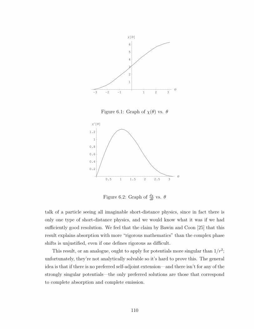
-3 -2 -1 1 2 3θ
1
2
3
4
5
6
χ@θD
radin.nb 1
Figure 6.1: Graph of χ(θ) vs. θ
0.5 1 1.5 2 2.5 3θ
0.2
0.4
0.6
0.8
1
1.2
χ @θD
radin.nb 1
Figure 6.2: Graph of dχdθ
vs. θ
talk of a particle seeing all imaginable short-distance physics, since in fact there is
only one type of short-distance physics, and we would know what it was if we had
sufficiently good resolution. We feel that the claim by Bawin and Coon [25] that this
result explains absorption with more “rigorous mathematics” than the complex phase
shifts is unjustified, even if one defines rigorous as difficult.
This result, or an analogue, ought to apply for potentials more singular than 1/r2;
unfortunately, they’re not analytically solvable so it’s hard to prove this. The general
idea is that if there is no preferred self-adjoint extension—and there isn’t for any of the
strongly singular potentials—the only preferred solutions are those that correspond
to complete absorption and complete emission.
110

-3 -2 -1 1 2 3θ
5
10
15
20
25
30χ@θD
radin.nb 1
Figure 6.3: Graph of (alleged) χ vs. θ in the weak regime
6.4 Experimental Realization
In 1998, Denschlag et al [23] realized a (basically quantum) 2D inverse square potential
experimentally. They studied the behavior of cold lithium atoms in a cylindrical
magnetic-optical trap (MOT), through the middle of which there was a thin wire.
They observed the number of atoms in the trap to decay exponentially, consistent with
the classical limit and also with the contraction semigroup treatment of the problem.
The important thing conceptually about this experiment is that it reminds us of the
diversity of boundary conditions that can be realized—there is nothing strange about
atoms being absorbed by a charged wire—and the corresponding breadth of sensible
solutions to a problem like the 1/r2 potential.
111
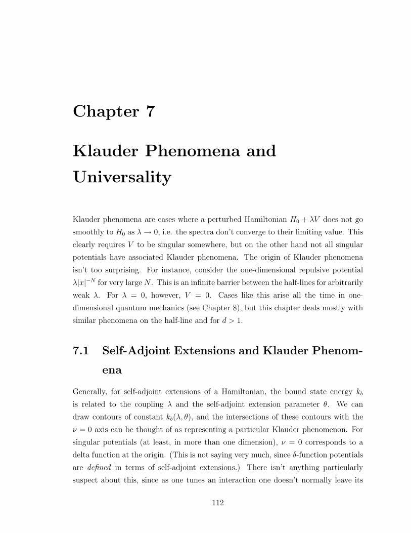
Chapter 7
Klauder Phenomena and
Universality
Klauder phenomena are cases where a perturbed Hamiltonian H0 + λV does not go
smoothly to H0 as λ→ 0, i.e. the spectra don’t converge to their limiting value. This
clearly requires V to be singular somewhere, but on the other hand not all singular
potentials have associated Klauder phenomena. The origin of Klauder phenomena
isn’t too surprising. For instance, consider the one-dimensional repulsive potential
λ|x|−N for very largeN . This is an infinite barrier between the half-lines for arbitrarily
weak λ. For λ = 0, however, V = 0. Cases like this arise all the time in one-
dimensional quantum mechanics (see Chapter 8), but this chapter deals mostly with
similar phenomena on the half-line and for d > 1.
7.1 Self-Adjoint Extensions and Klauder Phenom-
ena
Generally, for self-adjoint extensions of a Hamiltonian, the bound state energy kb
is related to the coupling λ and the self-adjoint extension parameter θ. We can
draw contours of constant kb(λ, θ), and the intersections of these contours with the
ν = 0 axis can be thought of as representing a particular Klauder phenomenon. For
singular potentials (at least, in more than one dimension), ν = 0 corresponds to a
delta function at the origin. (This is not saying very much, since δ-function potentials
are defined in terms of self-adjoint extensions.) There isn’t anything particularly
suspect about this, since as one tunes an interaction one doesn’t normally leave its
112
short-distance parts unchanged, but expects them to vary smoothly.
Assuming that potentials are continuous in the extended λ− θ plane, the limit as
λ→ 0 of any perturbation should be a δ-function. The physical reason for this is that
as you tune the coupling to zero the potential becomes very weak almost everywhere,
and since the wavefunctions are almost never within the central region of the potential
they are very slightly affected by the details of the interaction. (This is the same logic
we use a few sections down, while discussing universality in resonance phenomena.)
If this were true then all Klauder phenomena of the free Hamiltonian should be δ
functions. This would have severe consequences for any attempt to renormalize, say,
the 1/r2 potential by running the bound state against the global coupling. We know
from the treatment of Chapter 5 that, at least asymptotically, a regularized theory
reproduces the behavior of a self-adjoint extension. Therefore, taking the λ of a
regularized theory to zero with the energy kept constant is the same as following a
kb(λ, θ) contour, and should take you to a delta-function perturbation of H0 as you
take the coupling to zero. That is, for any of the regularization schemes of Chapter
4:
a→ 0 ⇒ ν → 0 ⇒ θ → θ0
for constant kb. This suggests that any such renormalization eventually reproduces a
point interaction—which is consistent with the fact that the bound state wavefunction
and the s-wave phase shift for the 2D “renormalized” inverse square potential are the
same as for the 2D delta function. This obviates the need for a renormalization
procedure, as well as calling its validity into question. We work out the 1/r2 example
again, and also demonstrate that the 1/x2 potential reproduces the 1D delta function
if you perform Chapter 4 renormalization on it. We also explicitly work the former
problem in the (λ, θ) plane.
Another application of these relations is to avoid Klauder phenomena by following
lines that pass through kb(0, θ0) = 0, which corresponds to no Klauder phenomenon.
The paths are generally not unique, but (as we shall see) a sensible parameterization
of short-distance physics picks one.
113
7.2 Examples
7.2.1 1/r2 in the Plane
Except for the factor of√kr this is the same as the 1D/3D case, so that
ψ(r) = Kiν(kr)
and under ch. 4 type renormalization the ground state wavefunction becomes
K0(kbr).
We can work out the s-wave phase shift as usual, by looking at the boundary con-
ditions for AJiν + BNiν . Since at the end we’re going to take ν → 0, the quantity
−B/A will, as usual, serve as tan δ. Using the hardcore cutoff scheme from Ch. 4,
AJiν(ka) +BNiν(ka) = 0
so that
−BA
=Jiν(ka)
Niν(ka)=
π(ka)iν/Γ(1 + iν)
(ka)iνΓ(−iν)− (ka)−iνΓ(iν).
With the assumption that Γ(1 + iν) ≈ 1 and a small-argument approximation, this
becomes
− iπν
1− (ka)−2iν
and, plugging in our renormalization rule ν = π/ log kba, this is
iπ2
log kba− log kbae−2πi log ka/ log kba.
The last of these expressions looks a little forbidding, but we know that as a→ 0,
log ka
log kba≈ log a
log a≈ 1
we can do a series expansion in the small quantity 1− log ka/ log kba. We can write
the argument of the exponential as
1−(
1− log ka
log kba
)in which case a first order Taylor expansion about e−2πi is
114
e−2πi − 2πi
(1− log ka
log kba
)and putting it all together,
−BA
=π
2 log kb/k
tan δ0 = π/2 log(kb/k),
which is, of course, the same as with δ2(r).
7.2.2 1/x2 on the Half-Line
The primary difference between the 1D and 3D (l = 0) Schrodinger equations is the
boundary condition that requires u(0) = 0 in three dimensions. A consequence is
that in one dimension an (even remotely well-behaved) attractive potential always
has a bound state, while in three dimensions that need not be the case. A more
mathematical way of stating the distinction is that one normally picks the Friedrichs
extension on R+− 0 when one is doing 3D quantum mechanics, but in one dimension
this extension is usually inappropriate for attractive potentials.
Suppose we regularize the potential with a square well at radius a. It is well-
known that a one-dimensional always attractive potential always has a bound state,
and since the only dimensional parameter is a, dimensional analysis suggests that the
bound state energy must go as 1/a2. To keep it fixed as a → 0 we have to scale λ
accordingly, so that we can take ζ = ν − 12
small for our purposes. The boundary
condition is
−qa tan qa =1
2+ ka
K ′ν(ka)
Kν(ka)
which simplifies, with the usual approximations (see Chapter 3), to
−λ =1
2− ν
[1− 2
Γ(−ν)Γ(ν)
(ka
2
)2ν].
Keep terms only to first order in ν we can reduce this expression to
−λ = 4ν(ka/2)2ν
115
which simplifies further to
kb =λ
a.
The bound state wavefunction flows to e−kx as ν → 1/2.
Now let’s consider the scattering states. The outside form of the wavefunction is
AH(1)ν (ka)−BH(2)
ν (ka) in terms of the Hankel functions, which we will refer to as H1
and H2. The inside wavefunction is a cosine because we’re working on the half-line
and we assume the problem is symmetric. Once again, the boundary condition is
(qa)2 =1
2+ k
AH ′1 −BH ′
2
AH1 −BH2
and, if we write the Hankel functions in terms of Bessel functions and take the ν → 0
limit, this becomes
λ =1
2+
1
2
(ka)3/2
i(A+B)
[(A−B)
(ka
2
)−1/2
− i(A+B)
(ka
2
)−3/2],
which is a nice form because two of the terms cancel out and what’s left is
−ikbk
=A−B
A+B
which is the result we expect for the 1D delta function. Therefore, the renormalization
procedure of Chapter 4 has left us once again with a point interaction.
There are infinitely many other ways to calculate the delta function in principle,
but most singular potentials are not exactly solvable so we won’t bother.
7.2.3 Self-Adjoint Extensions
It suffices to show that one can vary the coupling continuously from the strong regime
to the weak regime without losing self-adjointness at any stage, and without having a
discontinuity in the boundary condition. We know that there’s always an extension in
the weak regime, the critical regime, and the strong regime with a given bound state
energy kb 6= 0. So we can tune down the coupling and keep picking the appropriate
extensions. Our boundary conditions (in two dimensions) have the form
νψ + rψ′
νψ − rψ′=
Γ(−ν)Γ(ν)
(kbr
2
)2ν
For ν → 0 this simplifies to
116
νψ + rψ′
νψ − rψ′= −
(kbr
2
)2ν
and unless kb = 0 both sides approach the same limit. The boundary condition is
vacuous in the limit; however, since the limit exists from both sides and ψ is analytic
in ν at zero, one can think about this as a removable discontinuity, and plug in
the appropriate value of kb. Under a Chapter 4-type renormalization a strong 1/r2
potential flows up the kb contour to the critical value under renormalization; however,
we could just as well have done the critical problem directly. One might also point
out again that the critical problem isn’t in fact anomalous, if by that we mean that
there are no scale invariant boundary conditions. We would always choose the one
case for which the discontinuity is not removable is kb = 0.
This is also the only case for which the boundary condition isn’t vacuous in the
limit; it goes to rψ′(0) = 0, which is equivalent to throwing out the K0 solution.
How does one explain the disappearance of the Friedrichs extension in RG terms?
Suppose you have a potential with a running square well or delta function ring, and
turn up the coupling slightly past its critical value. The ground state does nothing
strange, because the rightmost zero of Kiν(x) is at about π/ν, which is within our
regularized core. However, the very shallow states—whose rightmost zeros are at
nπ/ν for arbitrarily large n, and which are therefore relatively unaffected by interior
behavior—appear near the threshold at this point. Of course, in practice there’s an
infrared cutoff too, so not quite. There will be regimes in any physical (no ultraviolet
or infrared divergencies) potential where the 1/r2 interaction is above critical strength
but there are no bound states.
A notable thing about the strong inverse square potential in two dimensions is
that it’s impossible to avoid a Klauder phenomenon, since you can’t get smoothly to
the Friedrichs extension by tuning the coupling to zero. Therefore any way of tuning
the coupling to zero leaves a bound state in the problem. Presumably this is generic to
strongly singular potentials, since the reason we can’t access the Friedrichs extension
has to do with the loss of the boundary condition. With singularities stronger than
1/r2 it’s also the case that one can’t get at any non-Friedrichs extensions from the
repulsive side, since the operators are self-adjoint and the wavefunctions vanish at
the origin; the critical value at λ = 0 is therefore highly nonanalytic. It’s physically
more evident in these cases that the Klauder phenomena must be generic, since as
you tune down the potential strength you also tune down its range, so that the bound
117
state finds itself less and less within the range of the interaction, and therefore less
and less sensitive to its details.
Finally, one should note that there can be no Klauder phenomena in l 6= 0 chan-
nels, because the limit as perturbation strength λ → 0 is self-adjoint. This fact
establishes Klauder phenomena as distinctively quantum mechanical, since the clas-
sical limit usually corresponds to l 1.
7.3 Nonanalyticity
Suppose you’re tuning up the depth of a square well: at the critical coupling just
before a new shallow bound state appears, there’s a zero-energy scattering resonance.
In contrast, there’s no such resonance in the critical 1/r2 interaction. This is an exam-
ple of the non-analytic dependence of some parts of the theory on coupling strength.
This non-analyticity is also characteristic of the 3D hydrogen atom, which has in-
finitely many bound states when it’s attractive but no resonance at zero coupling. In
both cases the non-analyticity takes place because we didn’t regularize the infrared
properties; however, the α/r4 potential [20], which has no infrared problems, has a
similar non-analyticity in its scattering length at α = 0.
An important thing about Klauder phenomena is that they are an example of
“non-analytic” (by which we mostly mean non-smooth) dependence of the spectra
on coupling at zero. A square well, in contrast, exemplifies “analytic” dependence.
With singular potentials we have drastic transitions at the points where they become
attractive, where the number of bound states goes up suddenly from 0 to ∞, and the
properties of the wavefunctions change drastically. Within a renormalization theory
framework, however, these transitions are artefacts of our theory, and the regularized
theory has no nonanalytic properties.
These nonanalyticities are a natural consequence of the universality of Klauder
phenomena. All singular perturbations must go to a delta function in the λ → 0
limit; however, most of them have infinitely many bound states for arbitrarily low
coupling, and the nonanalyticity comes from the disappearance of all bound states
but one to either −∞ or 0.
118
7.4 Universality
The renormalization group gives us a way to think about the universal asymptotic
features of a class of potentials, regardless of their short-distance structure. How-
ever, for the most part we have been dealing directly with motion in long-distance
potentials. A more striking instance of universality is the resonances of short-range
potentials. A standard result of scattering theory is that (in the s-wave channel) the
scattering length a→∞ for a potential with a very shallow bound state. One would
expect resonance phenomena to be generic for the same reason that one would expect
Klauder phenomena to be generic: the scattering length (or the width of a bound
state) is so much larger than the range of the potential that the effect could not pos-
sibly depend on the details of the interaction: most scattering particles go nowhere
near the core. The resonance phenomena of the two-body problem are relatively
straightforward [40]; however, a resonant three-body system exhibits the remarkable
Efimov effect.
7.4.1 Review of 3D Scattering
A key hypothesis of the usual scattering theory is that the scattering potential, or
scatterer, is spherically symmetric and localized. (This is not the case with Coulomb
or 1/r2 interactions, which need special treatment.) Let’s assume that this holds for
now. If we send in a waveform eikz = eikr cos θ, the steady-state solution at large
distances from the scatterer has two parts: the initial waveform and an outgoing
wave from the scatterer, which need not be spherically symmetric.
The expression
ψ(r, θ) = eikr cos θ + f(k, θ)eikr
r
holds asymptotically. f is called the scattering amplitude. The radial term is merely
a positive energy solution to the free particle Schrodinger equation, which holds when
we’re outside the range of the scatterer. The scattering cross section is the integral of
f over solid angle, and the scattering length is the zero energy limit of f . The partial-
wave analysis, which expands out the θ-dependence of z and f in terms of Legendre
polynomials, is a separation of variables in the scattering problem; its merit is that
it reduces the 3D problem to radial problems with angular momentum l. At low
energies, only the l = 0 (s-wave) equation matters; this is equivalent to saying that
at low resolution (long wavelength) everything looks spherically symmetric. Since,
119
in this case, the asymptotic behavior is governed by the free-particle Schrodinger
equation, the one asymptotic property that depends on the scatterer is the phase
shift of the eikr wave. The scattering amplitude for low-energy problems is related
to the phase shift as follows:
f(k) =1
k cot δ0(k)− ik.
δ0(k) must blow up as k → 0, to keep the scattering length finite; this is the case
with most sensible scatterers, such as the square well.
7.4.2 Bound States and Resonances
Bound states affect the behavior of the scattering problem bizarrely. Suppose you
tune the energy of your incoming s-wave for a fixed scatterer: tan δ0 always blows
up as the incoming energy approaches that of a bound state. This result is called
Levinson’s theorem, and is sometimes a useful way to count the bound states of a
system. (One can check that Levinson’s theorem holds for all the scattering problems
we work out; see also our discussion in Chapter 5.) A particularly important case
of Levinson’s theorem is when the bound state is very shallow, since then a→ −∞.
The physical origin of this effect is not entirely obvious, but what one sees in the
time-dependent picture is that the particle is almost trapped into a bound state, and
takes a long time to leave. The fact that the scattering length diverges is due to the
fact that bound states become less and less localized as their energy goes to zero,
since the asymptotic wavefunction e−kr/r falls away very slowly as k → 0. In fact, at
k = 0, the asymptotic wavefunction goes as 1/r.
The low-energy properties of systems near a resonance depend very slightly on
the nature of the internal attraction. In the bound state sector, this follows from the
fact that most of the bound state wavefunction is outside the range of the scatterer,
and the particle is hardly ever in the range of the forces. Of course, the system needs
to be exactly tuned for this to happen; in most cases the scattering length can be
obtained by dimensional analysis from the potential.
The scattering length is in some sense a measure of the spatial extent of the
shallowest bound state. Normally this is determined by k, which is determined by the
intrinsic scale of the potential; however, when k → 0 the scattering length diverges.
This connection is made carefully and explicitly in [40].
120

Note that this discussion is hopelessly invalid for the 1/r and 1/r2 potentials,
which have infinitely many arbitrarily shallow bound states.
7.4.3 Three-Body Scattering
The problem of three-body scattering is more intricate because of the greater number
of possible configurations. A two-body system is either bound or in the continuum;
but in a system of three interacting particles (let’s say particles 1, 2, and 3) there
are many more possibilities: for instance, two of the particles could be bound tightly
and separate from the third, or all three could be flying apart from each other, or
all three could be bound. Besides, all sorts of transitions—capture of 3 by the 1-2
system, which gets excited in the process; or deexcitation of 1-2-3 by the emission of
3, and other ways of sloshing energy about between the particles—are possible. The
problem is hard enough to think of in the time-dependent picture; in terms of the
time-independent picture it becomes even harder.
However, the physical basis for resonances is more intuitive in the three-body
problem. The idea is that a three-body bound state might be degenerate with a state
in which two of the particles are bound and the third is free. The third particle gets
held up by transition to the bound state, and takes a long time to leave the system.
This time-delay is the basic phenomenon; in the time-independent theory it shows
up—by means we will not discuss, but which can be found in textbooks [62]—as a
large phase shift.
7.4.4 The Efimov Effect
In the resonant two-body problem, there are no bound states; this is good, be-
cause there would be no relevant length parameter in the theory to describe their
spatial extent. However, Efimov [27] discovered in 1971 that there are infinitely
many shallow three-body states in a system of three identical, pairwise resonant
bosons. This is associated with the fact that the effective three-body potential for
this situation is inverse-square—in terms of the three-body “hyperspherical” radius
R =√r212 + r2
23 + r231—and strongly attractive. Since its discovery the Efimov effect
has been studied in great detail; a straightforward but long derivation is given in [40].
The surprising feature is that there are three-body bound states; the 1/r2 structure
follows from scale invariance, which follows from the absence of relevant dimensional
121
parameters. The argument that there are bound states is hard, but its conclusion
isn’t too implausible: if the two particles were almost bound without the third, then
their attractive interactions with the third particle ought to push them over the edge.
Once we know this much, we can use our treatment of the 1/r2 potential to deduce
most of the other properties of Efimov states: the level spacing, the single-parameter
dependence of the states, Efimov’s radial law [28], etc. As Ref. [40] notes, this
approach has a slight danger in that the separation of scales is not as clear in the three-
body problem as in the two-body problem. The issue is this: our treatments (and
Efimov’s) of the radial behavior of the problem have assumed that any probability
that goes into the inner region will come out again. This is not the case if deep two-
body states exist, because there’s a small chance that two of the particles will form a
deep bound state, which vanishes from the low-energy sector. Using the terminology
of Chapter 6, we can say that some of the probability is dissipated, and account for
this with the machinery of Chapter 6.
7.4.5 Consequences and Experimental Realization
Kraemer et al [39] recently observed the Efimov effect in an ultracold gas of cesium
atoms. The signature they detected was giant recombination loss, which had pre-
viously been predicted by [94], [40]. Suppose we have a three-body system with a
shallow pairwise bound state (equivalently, a large scattering length). The recombi-
nation rate is the rate at which a three-body bound state transitions into the state
consisting of a shallow two-body bound state and a free particle. At very low energies
recombination happens at a constant rate α. It turns out that the discrete scaling
symmetry of the problem manifests itself in log-periodic oscillations of the recombi-
nation rate in the Efimov regime. The recombination rate is pretty easy to measure
from the rate of loss of atoms (because of combination into shallow molecules) and the
temperature change due to the “anti-evaporation” [39] associated with the formation
of a two-body bound state.
122
Chapter 8
The One-Dimensional Hydrogen
Atom
There is some controversy as to what the phrases “hydrogen atom” and “Coulomb
potential” ought to mean in one dimension; the only problem we consider is the
following Hamiltonian:
H = − d2
dx2− λ
|x|(8.1)
The spectrum of this Hamiltonian has been argued over at some length in the liter-
ature. Loudon (1959) [98] found a ground state at E = −∞, and degenerate n > 0
states. Haines and Roberts (1969) [99] claimed that there were no degeneracies, but
a continuous negative-energy spectrum. Andrews (1976) [101] got rid of the ground
state by enforcing ψ(0) = 0, but his procedure reinforced the degeneracies. Hammer
and Weber (1988) [102] claimed that Loudon’s ground state was an “extraneous”
solution. Meanwhile, Gostev et al (1989) [104] discussed the potential from the point
of view of self-adjoint extensions. Gordeyev and Chhajlany (1997) [103] solved the
problem with Laplace transforms and semiclassical arguments, and decided that there
were neither degeneracies, nor a barrier, nor a ground state at −∞, nor an unspeci-
fied boundary condition, but that the one-dimensional hydrogen atom had the same
spectrum as the three-dimensional hydrogen atom. Tsutsui et al (2002) [95] worked
the mathematical problem using a technique equivalent to ours, but did not discuss
its physical interpretation.
We work the mathematical problem within a general discussion of the peculiarities
of 1D quantum mechanics. As treatments before this have found, the mathematical
123
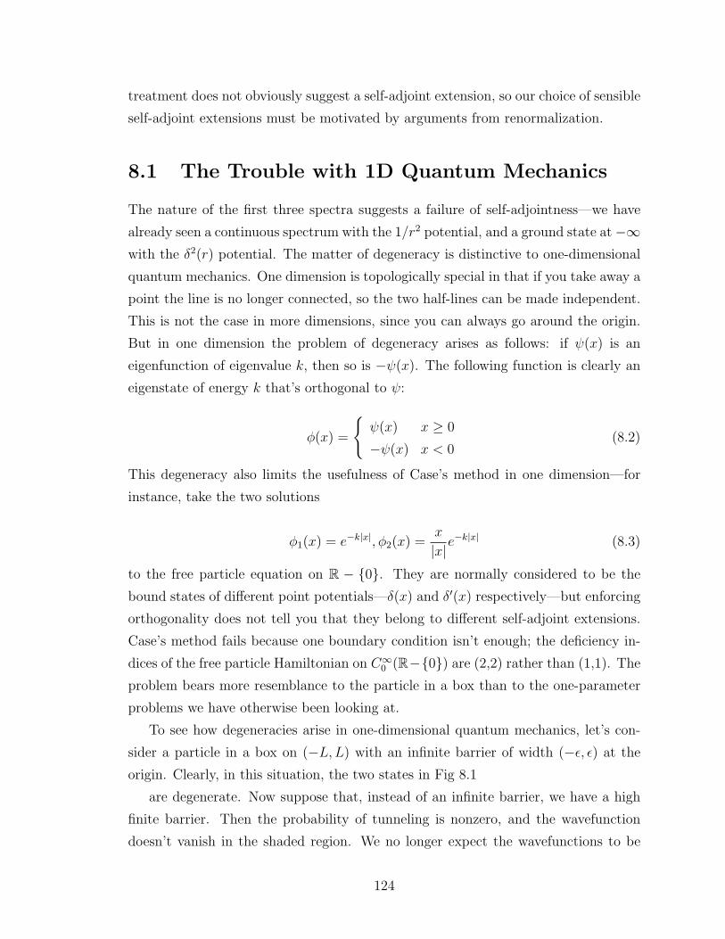
treatment does not obviously suggest a self-adjoint extension, so our choice of sensible
self-adjoint extensions must be motivated by arguments from renormalization.
8.1 The Trouble with 1D Quantum Mechanics
The nature of the first three spectra suggests a failure of self-adjointness—we have
already seen a continuous spectrum with the 1/r2 potential, and a ground state at−∞with the δ2(r) potential. The matter of degeneracy is distinctive to one-dimensional
quantum mechanics. One dimension is topologically special in that if you take away a
point the line is no longer connected, so the two half-lines can be made independent.
This is not the case in more dimensions, since you can always go around the origin.
But in one dimension the problem of degeneracy arises as follows: if ψ(x) is an
eigenfunction of eigenvalue k, then so is −ψ(x). The following function is clearly an
eigenstate of energy k that’s orthogonal to ψ:
φ(x) =
ψ(x) x ≥ 0
−ψ(x) x < 0(8.2)
This degeneracy also limits the usefulness of Case’s method in one dimension—for
instance, take the two solutions
φ1(x) = e−k|x|, φ2(x) =x
|x|e−k|x| (8.3)
to the free particle equation on R − 0. They are normally considered to be the
bound states of different point potentials—δ(x) and δ′(x) respectively—but enforcing
orthogonality does not tell you that they belong to different self-adjoint extensions.
Case’s method fails because one boundary condition isn’t enough; the deficiency in-
dices of the free particle Hamiltonian on C∞0 (R−0) are (2,2) rather than (1,1). The
problem bears more resemblance to the particle in a box than to the one-parameter
problems we have otherwise been looking at.
To see how degeneracies arise in one-dimensional quantum mechanics, let’s con-
sider a particle in a box on (−L,L) with an infinite barrier of width (−ε, ε) at the
origin. Clearly, in this situation, the two states in Fig 8.1
are degenerate. Now suppose that, instead of an infinite barrier, we have a high
finite barrier. Then the probability of tunneling is nonzero, and the wavefunction
doesn’t vanish in the shaded region. We no longer expect the wavefunctions to be
124
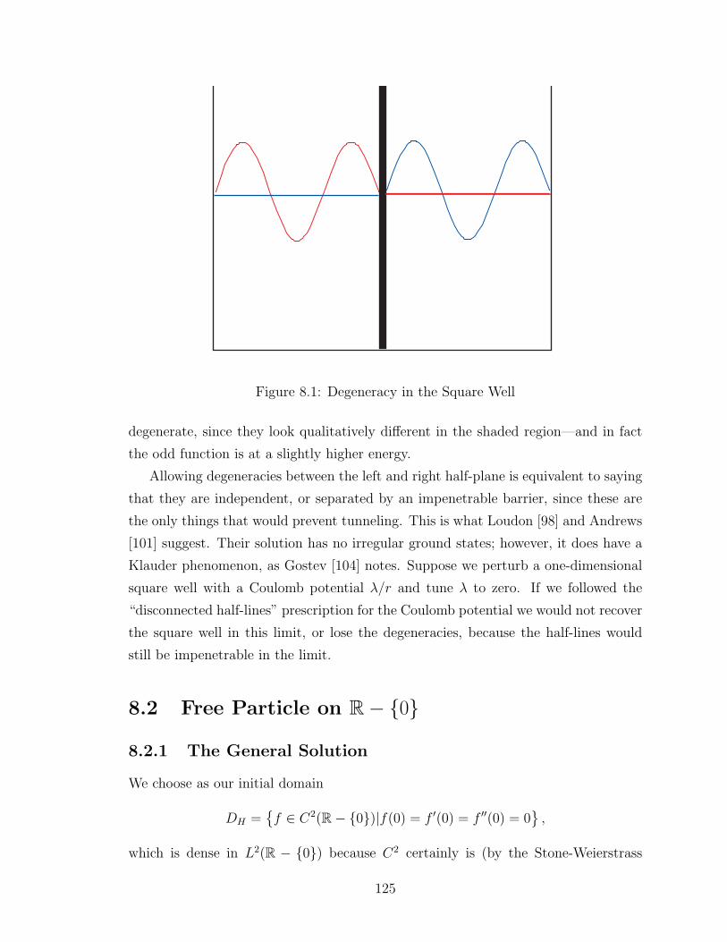
Figure 8.1: Degeneracy in the Square Well
degenerate, since they look qualitatively different in the shaded region—and in fact
the odd function is at a slightly higher energy.
Allowing degeneracies between the left and right half-plane is equivalent to saying
that they are independent, or separated by an impenetrable barrier, since these are
the only things that would prevent tunneling. This is what Loudon [98] and Andrews
[101] suggest. Their solution has no irregular ground states; however, it does have a
Klauder phenomenon, as Gostev [104] notes. Suppose we perturb a one-dimensional
square well with a Coulomb potential λ/r and tune λ to zero. If we followed the
“disconnected half-lines” prescription for the Coulomb potential we would not recover
the square well in this limit, or lose the degeneracies, because the half-lines would
still be impenetrable in the limit.
8.2 Free Particle on R− 0
8.2.1 The General Solution
We choose as our initial domain
DH =f ∈ C2(R− 0)|f(0) = f ′(0) = f ′′(0) = 0
,
which is dense in L2(R − 0) because C2 certainly is (by the Stone-Weierstrass
125
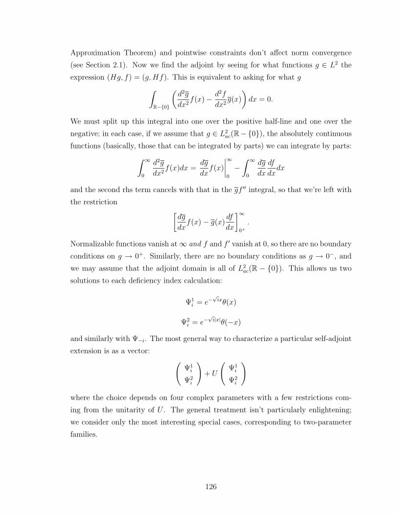
Approximation Theorem) and pointwise constraints don’t affect norm convergence
(see Section 2.1). Now we find the adjoint by seeing for what functions g ∈ L2 the
expression (Hg, f) = (g,Hf). This is equivalent to asking for what g∫R−0
(d2g
dx2f(x)− d2f
dx2g(x)
)dx = 0.
We must split up this integral into one over the positive half-line and one over the
negative; in each case, if we assume that g ∈ L2ac(R−0), the absolutely continuous
functions (basically, those that can be integrated by parts) we can integrate by parts:∫ ∞
0
d2g
dx2f(x)dx =
dg
dxf(x)
∣∣∣∣∞0
−∫ ∞
0
dg
dx
df
dxdx
and the second rhs term cancels with that in the gf ′′ integral, so that we’re left with
the restriction [dg
dxf(x)− g(x)
df
dx
]∞0+
.
Normalizable functions vanish at∞ and f and f ′ vanish at 0, so there are no boundary
conditions on g → 0+. Similarly, there are no boundary conditions as g → 0−, and
we may assume that the adjoint domain is all of L2ac(R − 0). This allows us two
solutions to each deficiency index calculation:
Ψ1i = e−
√ixθ(x)
Ψ2i = e−
√i|x|θ(−x)
and similarly with Ψ−i. The most general way to characterize a particular self-adjoint
extension is as a vector: (Ψ1i
Ψ2i
)+ U
(Ψ1i
Ψ2i
)
where the choice depends on four complex parameters with a few restrictions com-
ing from the unitarity of U . The general treatment isn’t particularly enlightening;
we consider only the most interesting special cases, corresponding to two-parameter
families.
126
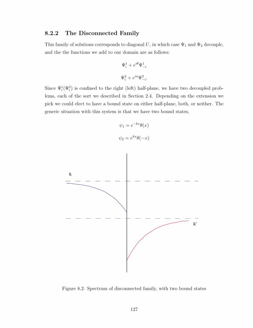
8.2.2 The Disconnected Family
This family of solutions corresponds to diagonal U , in which case Ψ1 and Ψ2 decouple,
and the the functions we add to our domain are as follows:
Ψ1i + eiθΨ1
−i
Ψ2i + eiφΨ2
−i.
Since Ψ1i (Ψ
2i ) is confined to the right (left) half-plane, we have two decoupled prob-
lems, each of the sort we described in Section 2.4. Depending on the extension we
pick we could elect to have a bound state on either half-plane, both, or neither. The
generic situation with this system is that we have two bound states,
ψ1 = e−kxθ(x)
ψ2 = ekxθ(−x)
k
k’
Figure 8.2: Spectrum of disconnected family, with two bound states
127
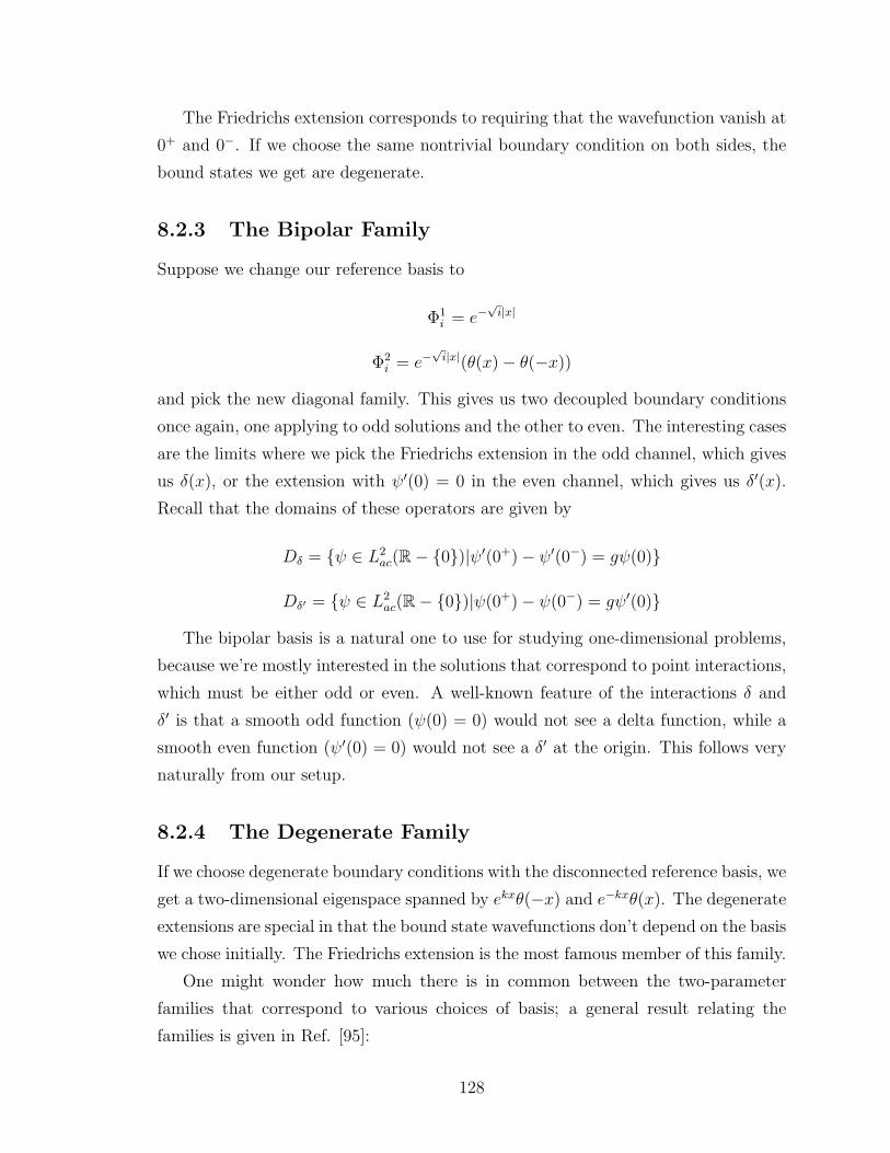
The Friedrichs extension corresponds to requiring that the wavefunction vanish at
0+ and 0−. If we choose the same nontrivial boundary condition on both sides, the
bound states we get are degenerate.
8.2.3 The Bipolar Family
Suppose we change our reference basis to
Φ1i = e−
√i|x|
Φ2i = e−
√i|x|(θ(x)− θ(−x))
and pick the new diagonal family. This gives us two decoupled boundary conditions
once again, one applying to odd solutions and the other to even. The interesting cases
are the limits where we pick the Friedrichs extension in the odd channel, which gives
us δ(x), or the extension with ψ′(0) = 0 in the even channel, which gives us δ′(x).
Recall that the domains of these operators are given by
Dδ = ψ ∈ L2ac(R− 0)|ψ′(0+)− ψ′(0−) = gψ(0)
Dδ′ = ψ ∈ L2ac(R− 0)|ψ(0+)− ψ(0−) = gψ′(0)
The bipolar basis is a natural one to use for studying one-dimensional problems,
because we’re mostly interested in the solutions that correspond to point interactions,
which must be either odd or even. A well-known feature of the interactions δ and
δ′ is that a smooth odd function (ψ(0) = 0) would not see a delta function, while a
smooth even function (ψ′(0) = 0) would not see a δ′ at the origin. This follows very
naturally from our setup.
8.2.4 The Degenerate Family
If we choose degenerate boundary conditions with the disconnected reference basis, we
get a two-dimensional eigenspace spanned by ekxθ(−x) and e−kxθ(x). The degenerate
extensions are special in that the bound state wavefunctions don’t depend on the basis
we chose initially. The Friedrichs extension is the most famous member of this family.
One might wonder how much there is in common between the two-parameter
families that correspond to various choices of basis; a general result relating the
families is given in Ref. [95]:
128
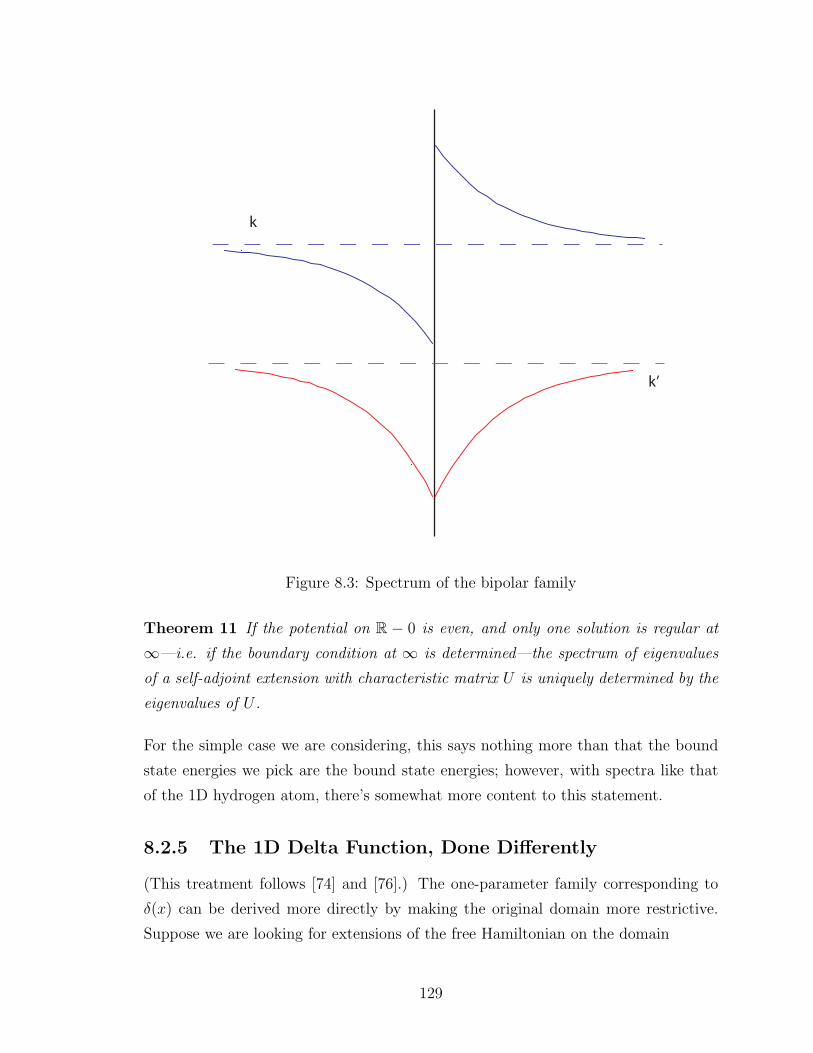
k
k’
Figure 8.3: Spectrum of the bipolar family
Theorem 11 If the potential on R − 0 is even, and only one solution is regular at
∞—i.e. if the boundary condition at ∞ is determined—the spectrum of eigenvalues
of a self-adjoint extension with characteristic matrix U is uniquely determined by the
eigenvalues of U .
For the simple case we are considering, this says nothing more than that the bound
state energies we pick are the bound state energies; however, with spectra like that
of the 1D hydrogen atom, there’s somewhat more content to this statement.
8.2.5 The 1D Delta Function, Done Differently
(This treatment follows [74] and [76].) The one-parameter family corresponding to
δ(x) can be derived more directly by making the original domain more restrictive.
Suppose we are looking for extensions of the free Hamiltonian on the domain
129

DH = ψ ∈ C∞(R)|ψ(0) = 0.
As before, we can find the adjoint domain by integrating the inner product and looking
at the expression [dg
dxf(x)− g(x)
df
dx
]∞0+
+
[dg
dxf(x)− g(x)
df
dx
]0−
−∞.
The first term vanishes because f(0) = 0, but since we have made no assumptions
about f ′(0), we can’t assume that the second term vanishes at zero. That is, the
requirement of symmetry gives us nontrivial information about g in this instance.
Our initial assumption of smoothness means that f ′ is continuous at zero, so the
expression reduces to
f ′(0)[g(0+)− g(0−)] = 0
and since f ′(0) is arbitrary, this constitutes a requirement that the wavefunction g
be continuous at the origin. So our adjoint domain could be written as
L2ac(R− 0) ∩ f ∈ L2(R)|f(0+) = f(0−).
Imposing this condition reduces the deficiency indices to (1, 1), since the only solution
that’s continuous at the origin is e−√ix, and the self-adjoint extensions yield the one-
parameter family of solutions corresponding to a delta function at the origin.
8.3 The 1D Coulomb Potential
8.3.1 Why We Need the Whole Family
Since 1xψ ∈ L2 iff ψ(0) = 0, the domain of the original Hamiltonian must be limited
to functions that vanish at the origin. However, for ψ ∈ DH , (ψ,H†φ) = (Hψ, φ)
is certainly well-defined for φ that don’t vanish at the origin, so clearly we need to
think about self-adjoint extensions. As we shall see shortly, some of the extended
domains do not require wavefunctions to vanish at the origin. This illustrates an
important feature of self-adjoint extensions, which is that the extended operator does
not always do quite the same thing as you would expect of the original operator, at
least at singularities.
130
8.3.2 Solving the Equation
If we substitute z = 2kx into the Schrodinger equation on the positive half-plane:
−(d2
dx2+λ
x
)ψ = −k2ψ (8.4)
it becomes
d2ψ
dx2+
λ
2kzψ − 1
4ψ = 0 (8.5)
which is a special case of Whittaker’s equation (AS 13.1.31). The solutions to this
equation are expressible in terms of confluent hypergeometric functions; the following
are a linearly independent pair:
Ψ1 ≡Mκ,1/2(z) = ze−z/2M(1− κ, 2, z) (8.6)
Ψ2 ≡ Wκ,−1/2(z) = e−z/2U(−κ, 0, z) (8.7)
(κ = λ/2k) Both functions are normalizable when κ is an integer, because the hy-
pergeometrics are polynomials in this case. (For these values, both solutions are also
linearly dependent). Otherwise, (AS 13.1.4)
Ψ1 ∼ ez/2z−κ−1
for large arguments. However,
Ψ2 ∼ e−z/2zκ (8.8)
which always decays fast enough to be normalizable. So we have a normalizable
solution on the half-plane for every negative energy; this is the continuum that Haines
and Roberts find, and we recognize it to be a symptom of non-self-adjointness. The
deficiency indices on the half-line are (1, 1).
Since the derivative diverges at the origin, we can’t do what we did with the
1D delta function. So we’re forced to extend the potential on R − 0 and pick
an appropriate family of extensions, as we did with the free particle. However, to
understand what we’re up against, we should first figure out how to extend the
problem on the half-line.
131
8.3.3 The Boundary Condition
The self-adjoint extension on the half-line is determined by the factor θ, and the
added wavefunction is
ψ = e−√ixU(−λ
√−i/2, 0,
√ix) + eiθe−
√−ixU(−λ
√i/2, 0,
√−ix). (8.9)
This is regular at the origin, since
U(a, 0, z) ≈ 1
Γ(1 + a)+ z log z
1
Γ(a)+ ξz
where ξ = 2γ − 1 + ψ0(1 + a), and the names of the constants don’t matter. On the
other hand, ψ′(x) is irregular at zero, and, to the crudest possible approximation,
log(√ix)
Γ(− λ2√i)
+ eiθlog(
√−ix)
Γ(− λ2√−i)
+ ξ(λ, θ)
If we divide the two forms near zero, we get that
U ′(a, 0, z)
U(a, 0, z)=
Γ(1 + a)
Γ(a)log z
What we want to do is, as usual, impose a condition on ψ′(x)/ψ(x) as x → 0. For
notational convenience we introduce −λ/2 = p. This way, we get
ψ(0) =1
Γ(1 +√ip)
+ e−iθ1
Γ(1 +√−ip)
=1
p
( √−i
Γ(√ip)
+e−iθ
√i
Γ(√−ip)
).
Now the other important thing is ψ′(0), which is undefined, so we want to look
at near-zero behavior. Note that a factor ofñi gets pulled out while taking the
derivative, so that
ψ′(x) ≈ log x
[ √−i
Γ(√ip)
+e−iθ
√i
Γ(√−ip)
]+ ξ
and, putting it all together, we see that
ψ′(x)
ψ(x)= 2p log x+ pµ.
And this can be rewritten as the boundary condition
ψ′(x)
ψ(x)+ λ log x = η(θ, λ) (8.10)
132
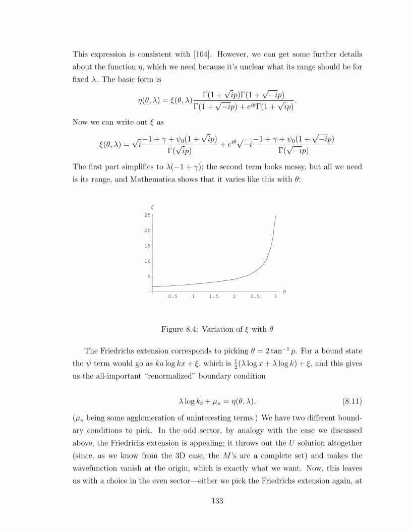
This expression is consistent with [104]. However, we can get some further details
about the function η, which we need because it’s unclear what its range should be for
fixed λ. The basic form is
η(θ, λ) = ξ(θ, λ)Γ(1 +
√ip)Γ(1 +
√−ip)
Γ(1 +√−ip) + eiθΓ(1 +
√ip)
.
Now we can write out ξ as
ξ(θ, λ) =√i−1 + γ + ψ0(1 +
√ip)
Γ(√ip)
+ eiθ√−i−1 + γ + ψ0(1 +
√−ip)
Γ(√−ip)
The first part simplifies to λ(−1 + γ); the second term looks messy, but all we need
is its range, and Mathematica shows that it varies like this with θ:
0.5 1 1.5 2 2.5 3θ
5
10
15
20
25
ξ
gostev.nb 1
Figure 8.4: Variation of ξ with θ
The Friedrichs extension corresponds to picking θ = 2 tan−1 p. For a bound state
the ψ term would go as ka log kx+ ξ, which is 12(λ log x+ λ log k) + ξ, and this gives
us the all-important “renormalized” boundary condition
λ log kb + µκ = η(θ, λ). (8.11)
(µκ being some agglomeration of uninteresting terms.) We have two different bound-
ary conditions to pick. In the odd sector, by analogy with the case we discussed
above, the Friedrichs extension is appealing; it throws out the U solution altogether
(since, as we know from the 3D case, the M ’s are a complete set) and makes the
wavefunction vanish at the origin, which is exactly what we want. Now, this leaves
us with a choice in the even sector—either we pick the Friedrichs extension again, at
133
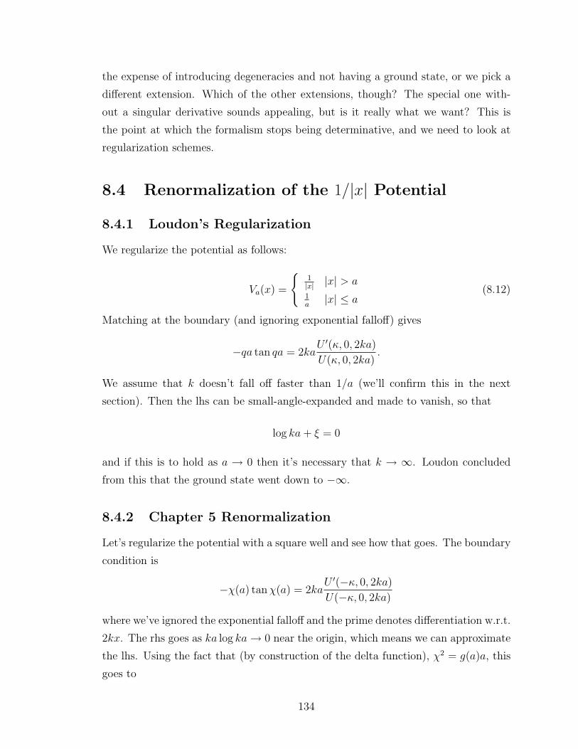
the expense of introducing degeneracies and not having a ground state, or we pick a
different extension. Which of the other extensions, though? The special one with-
out a singular derivative sounds appealing, but is it really what we want? This is
the point at which the formalism stops being determinative, and we need to look at
regularization schemes.
8.4 Renormalization of the 1/|x| Potential
8.4.1 Loudon’s Regularization
We regularize the potential as follows:
Va(x) =
1|x| |x| > a1a
|x| ≤ a(8.12)
Matching at the boundary (and ignoring exponential falloff) gives
−qa tan qa = 2kaU ′(κ, 0, 2ka)
U(κ, 0, 2ka).
We assume that k doesn’t fall off faster than 1/a (we’ll confirm this in the next
section). Then the lhs can be small-angle-expanded and made to vanish, so that
log ka+ ξ = 0
and if this is to hold as a → 0 then it’s necessary that k → ∞. Loudon concluded
from this that the ground state went down to −∞.
8.4.2 Chapter 5 Renormalization
Let’s regularize the potential with a square well and see how that goes. The boundary
condition is
−χ(a) tanχ(a) = 2kaU ′(−κ, 0, 2ka)U(−κ, 0, 2ka)
where we’ve ignored the exponential falloff and the prime denotes differentiation w.r.t.
2kx. The rhs goes as ka log ka→ 0 near the origin, which means we can approximate
the lhs. Using the fact that (by construction of the delta function), χ2 = g(a)a, this
goes to
134
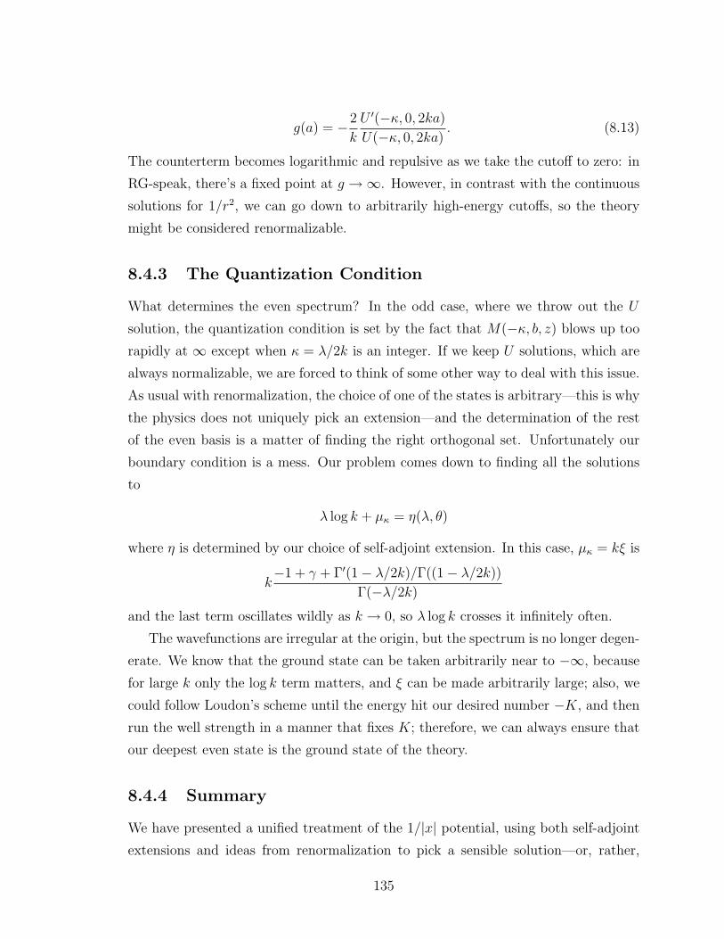
g(a) = −2
k
U ′(−κ, 0, 2ka)U(−κ, 0, 2ka)
. (8.13)
The counterterm becomes logarithmic and repulsive as we take the cutoff to zero: in
RG-speak, there’s a fixed point at g →∞. However, in contrast with the continuous
solutions for 1/r2, we can go down to arbitrarily high-energy cutoffs, so the theory
might be considered renormalizable.
8.4.3 The Quantization Condition
What determines the even spectrum? In the odd case, where we throw out the U
solution, the quantization condition is set by the fact that M(−κ, b, z) blows up too
rapidly at ∞ except when κ = λ/2k is an integer. If we keep U solutions, which are
always normalizable, we are forced to think of some other way to deal with this issue.
As usual with renormalization, the choice of one of the states is arbitrary—this is why
the physics does not uniquely pick an extension—and the determination of the rest
of the even basis is a matter of finding the right orthogonal set. Unfortunately our
boundary condition is a mess. Our problem comes down to finding all the solutions
to
λ log k + µκ = η(λ, θ)
where η is determined by our choice of self-adjoint extension. In this case, µκ = kξ is
k−1 + γ + Γ′(1− λ/2k)/Γ((1− λ/2k))
Γ(−λ/2k)and the last term oscillates wildly as k → 0, so λ log k crosses it infinitely often.
The wavefunctions are irregular at the origin, but the spectrum is no longer degen-
erate. We know that the ground state can be taken arbitrarily near to −∞, because
for large k only the log k term matters, and ξ can be made arbitrarily large; also, we
could follow Loudon’s scheme until the energy hit our desired number −K, and then
run the well strength in a manner that fixes K; therefore, we can always ensure that
our deepest even state is the ground state of the theory.
8.4.4 Summary
We have presented a unified treatment of the 1/|x| potential, using both self-adjoint
extensions and ideas from renormalization to pick a sensible solution—or, rather,
135
2 4 6 8 10λ
2 k
-3
-2
-1
1
2
3
4
5f
gostev.nb 1
Figure 8.5: The Quantization Condition. Intersections denote bound states.
a family of sensible solutions corresponding to different values of the ground state
energy. We have shown that in one-dimensional problems with parity where the
boundary condition at the origin is unspecified, there are in fact two sets of boundary
conditions to be applied: one for the even sector and another for the odd. We picked
a boundary condition to return the “intuitive” feature that the system ought to have
a ground state. The potential then behaves as if there were an added delta function
at the origin. (Such a perturbation would, of course, have no impact on odd states.)
The spectrum we found by this means was the same as that of Ref. [104].
Some previous authors (e.g. Gordeyev and Chhajlany [103]) rejected this spectrum
by claiming that it solved a different problem from the 1/|x|. However, we showed
by an EFT-type renormalization of the potential that the delta function term can
be derived from arguments identical to those that have been used quite widely to
study singular potentials. We do not wish to claim that our solution is the only
intelligible one—the widely accepted (Friedrichs) solution makes perfect sense if you
assume that there’s an impenetrable barrier at the origin. However, the logic that
derives this solution from the behavior of the Schrodinger equation “at the origin”
is inconsistent with a modern approach to singular potentials; from an EFT point
of view, it is hubristic to suppose that you know anything about this sector of the
theory. As long as the problem is strictly academic, one approach is no better than
another, but to the extent that this problem is physical the EFT approach is the only
sensible one, since we have no real knowledge of the short-distance physics involved.
136
8.5 Other 1D Potentials
8.5.1 The Strong 1/x2 Potential
In the strong regime this potential is pathological enough on the half-line; on the full
line one finds that it’s possible to have different sequences of boundary conditions
(and therefore of energy levels) for the even and odd sets of states. In this case
there’s no physical difference between the behavior of even and odd states about the
origin—they’re both oscillating infinitely fast—so the sanest extensions appear to be
the degenerate family.
8.5.2 Singular SUSY
For the potential
V (x) = ω2x2 +g
x2
on the half-line, a pair of independent solutions is
φ1(x) = xν+1/2e−ωx2/2M
(1
2+ν
4− k2
ω,1 + ν
2, ωx2
)
φ2(x) = xν+1/2e−ωx2/2U
(−1
2− ν
4+k2
ω,−1 + ν
2, ωx2
).
We could play the usual self-adjointness game with these. But as Lathouwers [105]
notes, there are two sets of orthogonal polynomials associated with the differential
equation. These are the following:
φn1 (x) = x1/2+νe−ωx2/2M
(1
2+ν
4−k2
1,n
ω,1 + ν
2, ωx2
)
φn2 (x) = x1/2−νe−ωx2/2M
(1
2+ν
4−k2
2,n
ω,1 + ν
2, ωx2
)Both sets are square integrable at the origin for 0 < ν < 1, and square integrable
at ∞ because the M ’s are polynomials at the appropriate values, so there’s a net
exponential falloff. We have two sets of boundary conditions to pick, and we consider
three possibilities. (A broader treatment is given in [95].)
137

The Friedrichs Extension
If we require that φ be “as regular as possible” at the origin, we must throw out
φ2. This gives us the Friedrichs extension, where the states are degenerate and the
wavefunctions are odd and even extensions of φn1 (x). The energy of the states is given
by En = 4n+2+2ν. (As usual, the Friedrichs extension maintains the lower bound of
the spectrum.) As we take the perturbation to zero, ν → 12
and the original spectrum
is not recovered: we find ourselves with only the odd states. The fact that the energy
of all the states is increased by an attractive perturbation is a little surprising, as is
the Klauder phenomenon.
The Anti-Friedrichs Extension
One could take the opposite tack and throw out all the φ1’s (I can’t think of a physical
motivation, but someone probably could.) The energy spectrum in this case is given
by En = 4n + 2 − 2ν, and as you tune the perturbation down you find that you’ve
lost the odd eigenvalues.
The Perturbative Extension
Or, as we’ve tended to do in this chapter, one could pick one of these extensions for
the even states and another for the odd. This has the generic advantage of lifting the
degeneracy between even and odd states. The spectrum is then 4n + 2 − 2ν for the
even states, and 4n+2+2ν for the odd. This choice is a particularly well-behaved one
because, as we take g → 0, the odd states go to 4n+ 3 and the even states to 4n+ 1,
and we get back the spectrum of the original harmonic oscillator. The implications
of these various choices for supersymmetry are discussed in the next chapter.
One of the nice things about this problem is that a naive analysis of the problem
using perturbation theory [105] automatically reproduces the “correct” result from
self-adjoint extensions. This might be tied to supersymmetry (see Chapter 9).
138
Chapter 9
Issues of Symmetry
The symmetries associated with the 1/r2 potential fall under two heads: scale in-
variance, which we saw a while ago, and supersymmetry. The latter applies only
to the weak regime; however, it has a tendency to “break” under self-adjoint ex-
tensions. This is not entirely surprising since, as Ref. [77] notes, even such trivial
symmetries as the parity invariance of the infinite well might break under self-adjoint
extensions. However, it’s interesting to see when and whether symmetries break un-
der self-adjoint extensions of singular potentials, because gauging the robustness of
symmetries is important in, say, field theory.
9.1 Anomaly Revisited
The operator Oa, defined as follows,
Oaf(x) = f(ax)
maps the domain of a scale-invariant Hamiltonian onto itself, since
H[Oaf(x)] = Hf(ax) =1
a2Haxf(ax) =
1
a2Hf,
and f ∈ D(H) by hypothesis. Suppose we operate on the domain of the strongly
attractive 1/r2 potential with O. Then
f(ax) ∼ cos(Ξ log(ax) +B) = cos(Ξ log x+B′),
where B′ = log a + B in general belongs to a different self-adjoint extension than
f(x). It follows that the domain of the self-adjoint Hamiltonian is necessarily not
139
scale invariant. Similar things can be said about the delta function and the weakly
attractive 1/r2 potential; however, in those cases, we do have one extension that pre-
serves scale invariance: the Friedrichs extension. (In the literature the delta function
is treated as an anomaly but the weak 1/r2 potential is not, though the problems are
in fact very similar. This is because the Friedrichs extension for a “delta function”
corresponds to a zero strength delta function, which most authors take to be no delta
function at all.)
We would expect very direct manifestations of the anomaly in the zero-energy
wavefunction, since Hψ = 0 has absolutely no scale in it. For the Friedrichs extension
of the inverse square potential with λ > −14,
ψ(0; r) = rν
and this is a solution even if we scale the coordinates. However, for λ < −14, the zero
energy wavefunction has the form
ψ(0; r) = sin(ν log r +B).
Under scaling of coordinates this collects a phase shift and becomes part of a different
self-adjoint extension, so we have lost scale invariance.
Once it has been shown that the domain of the Hamiltonian—and therefore the
Hamiltonian—is not scale-invariant, it might seem overkill to work any harder to
show that there is an anomaly. There is, however, an interesting algebra associated
with scale invariance.
The Algebra of Scale Invariance
The SO(2, 1) algebra associated with conformal invariance was first applied to this
problem by Jackiw [41]. We start by deriving Jackiw’s operator D.1 The unitary
operator that performs dilations, Uλ, is given by
Uλψ(x) =1
1 + λψ(x+ λx)
and if we suppose that U is generated by a dilation operator Λ, we can write infinites-
imal dilations as
1Our treatment, so far as it goes, is entirely different from Jackiw’s. He treats the transformations
as fundamentally acting on the time variable, whereas we work within the framework of the time-
independent Schrodinger equation.
140
(1 + iεΛ)ψ(x) =1
1 + εψ((1 + ε)x).
Assuming ψ to be nonpathological we can expand it around x to first order and get
ψ(x) + iεΛψ(x) = ψ(x) + εxψ′(x)− εψ(x)
and this simplifies to
iΛψ(x) = xψ′(x)− εψ(x)
which is to say that
Λ ≡ −xp− 1.
(We can also write this in Jackiw’s fashion as −(xp + px)/2, if we like.) Now we
commute this with the Hamiltonian:
[H, xp] = [H, x]p+ x[H, p]
[p2 + V (x), x]p+ x[p2 + V (x), p]
This simplifies to
[p2, x]p+ x[V (x), p]
which can be evaluated to be
2ip2 − ixdV
dx
using the position basis. Normally, xV ′(x) is not the same sort of thing as −2V ,
which is what we want; however, this is the case with the free particle (trivially), the
1/x2 potential, and the 2D delta function. So the commutator tidies up to
[Λ, H] = 2iH. (9.1)
There is another operator associated with these, Ω = x2, whose commutator with H
gives a quantity related to Λ:
[Ω, H] = 4iΛ (9.2)
141
Also,
[Ω,Λ] = −2iΩ. (9.3)
The symmetry we expect to be associated with Ω is the conformal symmetry x →x
1+ax. This transformation would send a state
ψ(x) → (1 + ax)ψ
(x
1 + ax
),
where the prefactor maintains the norm, and applying the same procedure as we did
for Λ we get
G = −ix+ ix2p,
which is no good. So it seems that the conformal symmetry isn’t a symmetry of the
time-independent problem.
Now we move to the time-dependent picture, where we have immediate problems
because the time-dependent Schrodinger equation says
dΛ
dt= [H,Λ] 6= 0,
Λ isn’t a constant of the motion. A way to get around that problem is to add an
explicit time dependence to Λ to cancel out the commutator. Doing this gives us
Jackiw’s operator D,
D = tH − (xp+ px)
4,
which is a constant of the motion. Similarly, the constant of motion associated with
Ω is
K = −t2H + 2tD +1
2x2,
which is called the conformal generator. The system closes under commutation:
i[D,H] = H, i[K,D] = K, i[H,K] = −2D.
This might look somewhat unfamiliar; however, if we make the following substitutions:
B = −D,A =H +K
2, C =
H −K
2
142
we get the much more transparent symmetry group generated by the algebra
i[A,B] = C,−i[B,C] = A, i[C,A] = B
which is SO(2, 1), the symmetry group associated with—among other things—Lorentz
transformations in 2+1 dimensions. De Alfaro et al [107] point out that H and K
correspond, in the standard basis, to rotations about lightlike axes.
These generators correspond directly to the symmetries of the time-dependent
theory that Jackiw [106] notes:
H : t → t+ δ
D : t → t(1 + δ)
K : t →(
t1+tδ
) (9.4)
These are respectively invariance under time translation, time dilation, and special
conformal transformations of the time variable. As Camblong [47] mentions, time
has units of length squared in our dimensions, so a dilation of time is automatically
a dilation of length.
The symmetry is broken because D ceases to correspond to a symmetry of the
theory. This shows up in the fact that the commutator i[D,H] = H (or, equivalently,
[Λ, H] = 2iH) breaks. To see how this happens, consider a small finite transformation
U = 1− iεΛ. The commutator of this with H is −iε[Λ, H]. H acts on the undilated
state and HU on the dilated state; since the transformation was infinitesimal rather
than discrete, these states cannot be in the same self-adjoint extension of H. There-
fore, the domain of [U,H]—and therefore of [Λ, H]—can include only those states
that are in all self-adjoint extensions of H, and it is impossible to pick a self-adjoint
H such that [Λ, H] = 2iH. This breaks the SO(2, 1) algebra, and constitutes the
anomaly discussed by Camblong et al [44].
9.2 A Ladder Operator?
The repulsive and 1/x2 potential have features in common with the harmonic oscilla-
tor, as we will discuss, and it’s possible to define structures similar to ladder operators
for them. As ladder operators these are fairly useless because there aren’t any bound
states. For λ < −14
we lose the operator structure, but we do have a tower of bound
states. We know we can’t define a number operator for this situation, because the
143
system has no ground state. However, in practice we know how the operators work;
the raising operator takes a bound state KiΞ(kx) to the state KiΞ(eπ/Ξkx). Therefore
the raising and lowering operators are discrete dilation operators, of the form
A± = e±iΛ(Ω−1),
where Ω = π/Ξ. We can deduce the commutators [A±, H] from their operation on
an arbitrary state.
[H,A]φ(x) = HAφ− AHφ =1
ΩHφ(Ωx)− AHφ(x)
We can do this explicitly for our scale invariant Hamiltonian by noting that Hφ(x) is
just some function Ψ(x), so we can apply A to it by simply replacing all the x’s with
Ωx’s.
ΩHAφ(x) = − d2
d(Ωx)2φ(Ωx) +
λ
Ω2x2φ(Ωx) = −φ′′(Ωx) +
1
Ω2x2φ(x)
This is just (Ω2 − 1)Hφ(Ωx) = (Ω2 − 1)HAφ(x), and it follows that
[H,A] = (Ω2 − 1)HA.
To see that A is a sort of lowering operator, consider its action on an eigenstate of
energy E.
AΨ =1
EAEΨ =
1
EAHΨ =
1
Ω2EHAΨ.
Therefore AΨ is an energy eigenstate of H with eigenvalue EΩ2.
9.3 Supersymmetry
(This treatment follows Das and Pernice [49] closely; I have tried to reinterpret their
work in terms of self-adjoint extensions.)
The Hamiltonian for the simple harmonic oscillator can be written in dimensionless
units as
H =~ω2
(P 2 + ω2Q2)
where Q = x√mω/~ and P = p/
√mω~. If we write A = Q + iP (in which case
A† = Q− iP since both operators are Hermitian) we can write the Hamiltonian as
H =~ω2
(AA† − 1) =~ω2
(A†A+ 1)
144
and we’ll call the prefactor 1. In these units the energy spacing is 2 and the ground
state for the SHO is at 1. The product A†A ≡ N , the number operator, and the
three operators have the following commutation relations:
[A,A†] = 1, [N,A] = −A, [N,A†] = A†
The first of these properties follows from [x, p] = i~; the other two follow from the
first. These properties make the oscillator very easy and elegant to solve. That’s not
all that it’s good for; in fact, it’s tremendously deep and important, though we won’t
do much more than graze the iceberg. Consider the two Hamiltonians
H+ = N + 1 = A†A
H− = N − 1 = AA†
Evidently H+ = H− + 2. So the spectrum of H+ is 2, 4, 6... and that of H− is
0, 2, 4.... That is, the spectra of H+ and H− are identical except for a zero-energy
ground state that H− has and H+ does not. Potentials with this structure are said
to be supersymmetric (SUSY) partners. Note that the degenerate states merely
have the same energy; they do not look alike; in fact they’re of opposite parity. The
origin or point of this symmetry might seem obscure in quantum mechanics; however,
it’s an important symmetry in QFT and a familiar word to most physicists. The hope
is that understanding the properties of SUSYQM—especially whether and how it is
broken—might help us understand the same issues in field theory.
The almost-degeneracy of the spectrum is independent of what A and A† are.
Suppose
H−Ψ = AA†Ψ = EΨ
It follows that
H+(A†Ψ) = A†AA†Ψ = A†EΨ = E(A†Ψ)
i.e. we have an eigenstate of H+ with exactly the same eigenvalue. (We can run the
same thing in reverse using Q.) The exception to this logic is if either A or A† applied
to a state ψ in the Hilbert space gives a trivial state. If we assume that A = W + iP ,
where W (x) is some function of x called the superpotential, we give a quick and
sloppy argument to show that it’s impossible for both conditions to hold at once.
Suppose Aψ = 0 and A†φ = 0:
145
dψ
dx= −Wψ (9.5)
dφ
dx= Wφ (9.6)
dψ
ψ= −dφ
φ(9.7)
and therefore
ψ ∼ 1
φ
so it’s impossible for both of them to be normalizable.
Supersymmetry is said to hold when either of the solutions is normalizable; a
mechanism that can potentially break supersymmetry is the imposition of boundary
conditions that take the ground state out of the operator domain. This is how self-
adjoint extensions come into the picture.
9.3.1 Supersymmetric Oscillator on the Half-Line
Suppose you take the harmonic oscillator on the half-line and put an infinite wall at
the origin. This throws out the even states, so that the bound state for our harmonic
oscillator is now at 3 and the spectrum is 3, 7, 11, .... For a supersymmetric pair,
this would mean that the spectra were 4, 8, 12, ... and 2, 6, 10, ..., and this is not
a supersymmetric pair. Das and Pernice show that this is an artefact of our regular-
ization scheme, which breaks supersymmetry between H+ and H−. They regularize
the problem in a way that retains the symmetry; this leads to a supersymmetric
spectrum, but adds delta function terms to the boundary. In terms of self-adjoint
extensions, this means that the supersymmetric partners are not necessarily in the
“same” self-adjoint extension. This is all right since AA† and A†A are not the same
operator.
Supersymmetry is different from, say, scale invariance in that it’s a spectral prop-
erty; it makes sense to talk about the spectrum only after you’ve chosen a self-adjoint
extension. However, the forms of the Hamiltonians are determined by the superpoten-
tial W , so it’s reasonable to ask whether, for a supersymmetric pair, one is guaranteed
that there will be at least some self-adjoint extension for which the spectra are super-
symmetric. In the case of the half oscillator, there is; if we impose ψ′(0) = 0 on H−
146
and ψ(0) = 0 on H+, we get back a supersymmetric pair whose spectra are identical
to those of the full oscillator restricted to the half-line.
The regularization scheme they choose works as follows. The superpotential is
W = xθ(x) on the half-line, so they approximate it by Wa = xθ(x) + aθ(−x) and
take the limit as a → +∞. If we write V± as the potential terms of H±, these work
out to be
V+ = x2θ(x) + a2θ(−x)− xδ(x)− aδ(x)− θ(x)
V− = x2θ(x) + a2θ(−x) + xδ(x) + aδ(x) + θ(x)
and of course xδ(x) vanishes at the origin. As a → ∞, the boundary conditions are
set mostly by the δ-function terms, which become strongly repulsive for V+—which
acquires a Dirichlet boundary condition at the origin—and strongly attractive for V−.
In the limit, as Das and Pernice show, this system is supersymmetric.
The disadvantage of their scheme is that they implicitly assume that SUSY holds
at all scales. Since we don’t know that short-distance physics is supersymmetric, it
seems overoptimistic to suppose that no explicit symmetry breaking occurs. How-
ever, within its limits the technique of Das and Pernice is robust, since a regularized
superpotential will always generate supersymmetry, and this should hold in the limit
as long as the potential isn’t too pathological.
9.3.2 The x2 + 1/x2 Potential
Consider the superpotential W (x) = gx− x. The operators associated with this are
A =
(− d
dx+g
x− x
)
A† =
(d
dx+g
x− x
).
The Hamiltonians can be calculated from this:
H+ = A†A = − d2
dx2+g2
x2+ x2 − g
x2− 2g − 1
H− = AA† = − d2
dx2+g2
x2+ x2 +
g
x2− 2g + 1
The couplings of the inverse square terms are always in the weak regime; for
g(g ± 1) < −1/4 we must have g complex, but in that case A and A† would fail to
147
be adjoints and all hell would break loose. In fact, this potential has issues even in
the weak regime, since the Friedrichs extension is justifiable only for λ > 0,2 and for
any λ < 0 our choice of ground state is arbitrary. However, from the point of view
of supersymmetry this is as much of an opportunity as a problem, since it means
that we can put in a zero-energy ground state by hand. This is possible only if
λ < 3/4, |g| < 1/2, which holds either for both Hamiltonians or for neither. The
reason for this restriction is that if λ > 3/4 we have an impenetrable barrier at the
origin; the only regular wavefunction is the one that vanishes. This gives us a twofold
degenerate spectrum of bound states on the line, and supersymmetry is broken for
the same reason as with the cutoff we discussed earlier.
However, for weak g one can use perturbation theory to solve the potential [105].
Let’s assume, without loss of generality, that g > 0. As we have seen, a careful
treatment using self-adjoint extensions gives a family of which a very small subset
are consistent with perturbation theory; the method of Lathouwers picks one of these
automatically. That the direct treatment works is a consequence of the theory of
orthogonal polynomials, which Lathouwers uses. Anyway, the sensible/perturbative
spectrum has two series of levels (α = 12
√1− 4λ):
E±n = 2(2n± α+ 1)
φαn(x) = xα+1/2e−x2/2Lαn(x
2)
and the even (E−n ) [resp. odd (E+
n )] wavefunctions are even [odd] extensions of φ(x)
to the negative half-plane.
There’s also an algebraic solution to the problem, which Das and Pernice supply.
One can look for a state of vanishing energy by solving Aψ = 0. As a first-order
equation, this is relatively easy, and
ψ ≈ xge−x2/2
so we have picked the self-adjoint extension that gives us a bound state at zero energy.
Which extension does this correspond to? Regardless of which potential possesses this
state, V+ has been translated down from its canonical position, so what we’re looking
for is a ground state of the oscillator plus well system at 1 + 2g. Since 2g < 1 this is
too low to be a bound state of the Friedrichs extension. By the method of Lathouwers
2It’s not required in any case; the barrier need not be impenetrable.
148
the bound state of the perturbative extension is 2(1−α) = 1+2g, which is just what
we wanted.
Does the rest of the spectrum line up? The first odd state goes to 2 + 2α =
3− 2g. Translating it down takes it to 2− 4g. For V− the first bound state using the
Lathouwers extension is at 1− 2g before translating; on translating by 1− 2g it goes
to 2− 4g and lines up perfectly with the first excited state of V+. The rest is left to
the reader’s imagination.
Of course, one should be careful about saying that SUSY is “preserved” under the
Lathouwers extension. SUSY is, in quantum mechanics at least, basically a duality
relationship; and a better phrasing might be that one way to make a formally SUSY
pair of the x2 + 1/x2 type have supersymmetric spectra is to take the Lathouwers
extension of both operators. One might speculate that the existence of a Lathouwers
extension is related to the problem’s being supersymmetric.
9.4 Virasoro Algebra of the 1/x2 Potential
We didn’t need the harmonic oscillator term to make the 1/x2 potential factorizable.
The relevant operators are
A = − d
dx+g
x,A† =
d
dx+g
x.
These produce the Hamiltonians
H+ = AA† = − d2
dx2+g(g + 1)
x2
H− = A†A = − d2
dx2+g(g − 1)
x2
and commute as follows:
[A,A†] =2g
x2
[A†, H] =−2g
x2A†
[A,H] =2g
x2A
So the Hamiltonian is not a number operator. None of this works for strong coupling,
since that would require g ∈ C, in which case the operators A and A† would fail to
149
be adjoints, and the product AA‡, where A‡ is the true adjoint of A, would not be a
legitimate Schrodinger Hamiltonian.
As well as the generator of the SO(2, 1) group, this Hamiltonian has another
algebra associated with it, called a Virasoro algebra, which Ref. [42] uses to discuss
the scaling properties of black holes. Virasoro algebras are of great importance in
string theory; we mention this one mainly for completeness. Let’s suppose that
Ln = −xn+1 ddx
and Pm = 1/xm. (It’s easy to see that the Hamiltonian can be written
as AA† = (−L−1 + gP1)(L−1 + gP1). The generators Lm and Pn form the following
algebra:
[Pm, Pn] = 0
[Lm, Pn] = nPn−m
[Lm, Ln] = (m− n)Lm+n +c
12(m3 −m)δm+n,0
[Pm, H] = m(m+ 1)Pm+2 + 2mL−m−2
[Lm, H] = 2g(g − 1)P2−m − (m+ 1)(L−1Lm−1 + Lm−1L−1
are easy to establish, except for the last term in the third commutator, which is
an “extension” of the algebra. Birmingham et al study the representations of this
algebra, and possible extensions of it to the strong-coupling case; however, their main
interest is in the weak sector. Their remarks on self-adjoint extensions are somewhat
surprising; for example, they claim that the Hamiltonian with ν = −1/4 (i.e. the 2D
delta function) has infinitely many bound states with wavefunctions ψ =√xK0(knx).
This is clearly inconsistent with the requirement that the operators be self-adjoint,
since K0 is nodeless and definitely cannot be made orthogonal to itself by dilation.
(After all, δ2(r) does not have infinitely many bound states.)
150
Chapter 10
Summary and Applications
Renormalization theory teaches us that deep down all singular potentials are normal
and solvable, and that one doesn’t need to know the details of their short-distance
behavior to solve them. Suppose short-distance physics comes into play at a length
scale ε. Then for particles with energy k2 1/ε2, such physics manifests itself only as
a boundary condition. The spectrum depends on the boundary condition, which has
two implications—first, that we can’t ignore it; and second, that we can determine
the boundary condition by experimental observation of the spectrum.
So what we need is an effective theory that involves nothing more than the long-
distance physics and the boundary condition (or the experimental observable), and
gives accurate predictions for low-energy observables. There are two ways to do this.
The more explicit one is renormalization, in which one picks a parameterization of
short-distance physics (a square well, say) and explicitly replaces the details of the
short-distance theory with a boundary condition. This is a procedure we have used
in Chapter 5; we scale the short-distance physics as the long-distance physics goes to
zero to keep the observable constant. The other way is to use the procedure of self-
adjoint extensions, which involves applying the boundary condition directly to the
operator’s domain. These methods are equivalent because a square well in the limit
ε→ 0 is a smeared-out point interaction, and (as we have seen) point interactions can
be written as self-adjoint extensions. One should note that self-adjoint extensions do
not give an accurate description of the theory all the way down; their predictions are
valid only to the extent that they coincide with renormalization, which is to say, for
k 1/ε, where ε is the distance down to which we know what’s going on.
Each of these methods has its limitations: self-adjoint extensions can be difficult
151
to calculate, and renormalization schemes might produce scheme-specific effects. (An
example is the continuous paths of Chapter 5.) In addition, as we saw in the case
of one-dimensional quantum mechanics, there are often self-adjoint extensions that
do not correspond to a realistic parameterization of short-distance physics; renormal-
ization is sometimes necessary to find the good extensions. In the one-dimensional
problem, this might mean throwing out solutions with discontinuous wavefunctions.
The link between renormalization and self-adjoint extensions means that any
symmetry in the self-adjoint extensions must manifest itself asymptotically in the
renormalized theory. An example is the discrete scale symmetry of the strong 1/r2
potential. This symmetry also manifests itself in the log-periodic dependence of short-
distance physics on the cutoff radius, which we call a limit cycle.
An interesting feature of very singular potentials is that no continuous scaling of
short-distance physics with a works for arbitrarily small a. Physically this means that
you can’t keep, say, the ground state fixed under renormalization. This corresponds
to the fact that the self-adjoint extensions have spectra unbounded from below, so
as you take the cutoff to zero, bound states keep appearing near the bottom of your
spectrum. What saves renormalization in this case is that a boundary condition
is (asymptotically) fixed by requiring a bound state to be at a given energy, and
it doesn’t matter at all what the state number is. This is related to the notion
of the privacy of deep bound states, which I have shown in the case of scattering
observables—the presence of deep, localized bound states does not affect low-energy
scattering at all. This is analogous to classical wave mechanics, where you need high
frequency (high energy) waves to detect and resolve small features.
Another generic feature of singular potentials is the so-called Klauder phenomenon,
where a potential V is sufficiently singular that H0+λV does not return the spectrum
of H0 as λ→ 0. We have explained Klauder phenomena—or at least the class associ-
ated with singular potentials—in terms of self-adjoint extensions of the free-particle
Hamiltonian, and therefore in terms of delta functions. The origin of these phenom-
ena becomes a lot clearer if one thinks of them in terms of the variation of boundary
conditions as one alters the coupling. We argue (a) that Klauder phenomena are
generic, and (b) that renormalizing the coupling of singular potentials—a technique
quite widely used in the literature—produces a Klauder phenomenon, and therefore
produces generic results that have nothing to do with the potential used.
We have worked mostly with exactly solvable potentials, because those are the
152

only cases for which self-adjoint extensions can be calculated exactly and compared
with the results of various renormalization schemes.
10.1 Singular Potentials in Physics
This is a brief catalogue of some places where singular potentials and failures of self-
adjointness are interesting, beyond the two-body Schrodinger equation. We omit the
Efimov effect and the charged wire experiment, which have already been discussed.
10.1.1 The Relativistic Coulomb Problem
The Dirac equation for relativistic spin-1/2 particles in a Coulomb potential can be
written as follows [1]:
du
dr− χ
u
r=
(1− E − αZ
r
)w(r)
dw
dr+ χ
w
r=
(1 + E +
αZ
r
)u(r)
where (u,w) are the components of the spinor field, χ is a (half-integer) angular
momentum quantum number, and αZ is the nuclear charge. We can already see the
beginnings of trouble in the fact that the potential term scales with the derivative
term. Case [1] rewrites this equation in terms of a new set of variables as follows:
d2ψ
dρ2+
(1
ρ− 1
)dψ
dρ+
(Eδ
ρ+α2Z2 − χ2
ρ2
)ψ = 0.
When α2Z2 − χ2 > 14, i.e. if the nucleus is sufficiently highly charged, we have the
usual pathologies of the inverse square potential.
Similarly, the Klein-Gordon equation for spin-0 particles can be rewritten as a
Schrodinger equation:
d2u
dr2+
(−(1− E2) +
2EαZ
r+α2Z2 − l(l + 1)
r2
)u = 0
and this has the same features.
An early attempt to apply dimensional regularization to the pathologies of the
relativistic Coulomb problem is in Ref. [87], but it has occasioned some controversy
[88]. Another interesting paper is Ref. [26], which relates Case’s method to absorptive
solutions by changing the inner product relative to which self-adjointness is calculated.
153
10.1.2 Solvable Models with Singular Interactions
The most famous example is the Kronig-Penney model, which models an atomic
lattice by a one-dimensional array of delta functions. This model, despite its sim-
plicity, can reproduce the electronic band structure of crystals. For the details, see
Ref. [53]. Two classes of one-dimensional models in condensed matter physics, the
Calogero-Sutherland models [13] and the Haldane-Shastry models ([108],[109]),
have inverse square interactions. A Calogero-Sutherland model was recently realized
with ultracold Bose atoms [110]. In addition to these, several shape invariant and
exactly solvable potentials, such as the Poschl-Teller and Rosen-Morse potentials,
have interactions that are inverse square at certain scales (for details see [91]).
10.1.3 Dipoles and Black Holes
These applications are discussed in Ref. [44]. A familiar fact from electrodynamics
is that a point dipole produces a 1/r2 potential. One would expect to find a critical
strength for the 1/r2 potential to have bound states. This has been verified exper-
imentally for electrons and polar molecules. Another application is in the study of
the near-horizon structure of black holes, which can be modeled by a 1/r2 potential
in certain regimes [44],[42].
10.2 Executive Summary
We could have summed up the contents of this rather long thesis in the following
equivalences:
• Self-Adjoint Extensions = Some Renormalization Schemes
• Other Renormalization Schemes = Delta Functions
• Boundary Conditions = Absolutely Anything
However, brevity 6= intelligibility.
154
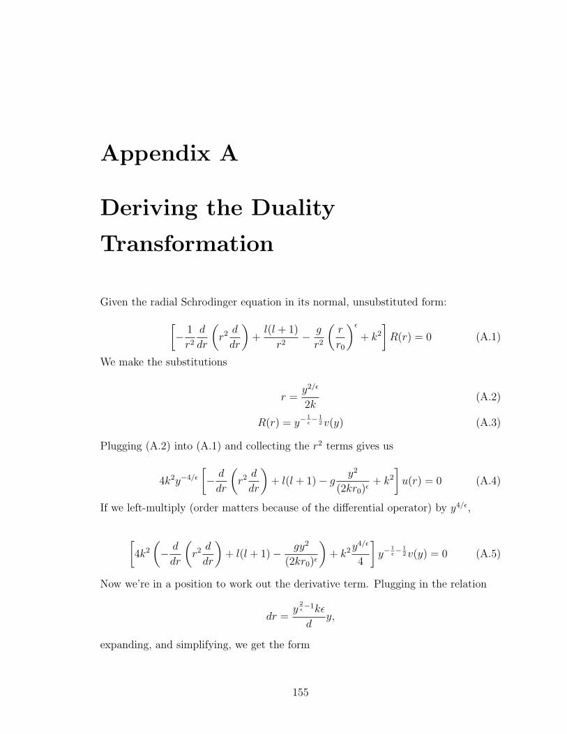
Appendix A
Deriving the Duality
Transformation
Given the radial Schrodinger equation in its normal, unsubstituted form:[− 1
r2
d
dr
(r2 d
dr
)+l(l + 1)
r2− g
r2
(r
r0
)ε+ k2
]R(r) = 0 (A.1)
We make the substitutions
r =y2/ε
2k(A.2)
R(r) = y−1ε− 1
2v(y) (A.3)
Plugging (A.2) into (A.1) and collecting the r2 terms gives us
4k2y−4/ε
[− d
dr
(r2 d
dr
)+ l(l + 1)− g
y2
(2kr0)ε+ k2
]u(r) = 0 (A.4)
If we left-multiply (order matters because of the differential operator) by y4/ε,
[4k2
(− d
dr
(r2 d
dr
)+ l(l + 1)− gy2
(2kr0)ε
)+ k2y
4/ε
4
]y−
1ε− 1
2v(y) = 0 (A.5)
Now we’re in a position to work out the derivative term. Plugging in the relation
dr =y
2ε−1kε
dy,
expanding, and simplifying, we get the form
155
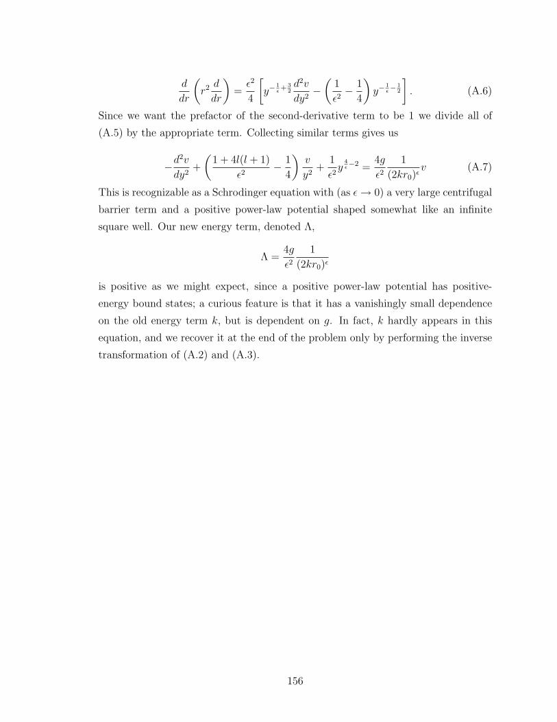
d
dr
(r2 d
dr
)=ε2
4
[y−
1ε+ 3
2d2v
dy2−(
1
ε2− 1
4
)y−
1ε− 1
2
]. (A.6)
Since we want the prefactor of the second-derivative term to be 1 we divide all of
(A.5) by the appropriate term. Collecting similar terms gives us
−d2v
dy2+
(1 + 4l(l + 1)
ε2− 1
4
)v
y2+
1
ε2y
4ε−2 =
4g
ε21
(2kr0)εv (A.7)
This is recognizable as a Schrodinger equation with (as ε→ 0) a very large centrifugal
barrier term and a positive power-law potential shaped somewhat like an infinite
square well. Our new energy term, denoted Λ,
Λ =4g
ε21
(2kr0)ε
is positive as we might expect, since a positive power-law potential has positive-
energy bound states; a curious feature is that it has a vanishingly small dependence
on the old energy term k, but is dependent on g. In fact, k hardly appears in this
equation, and we recover it at the end of the problem only by performing the inverse
transformation of (A.2) and (A.3).
156

Bibliography
[1] K.M. Case, “Singular Potentials,” Phys. Rev. 80(5), 797 (1950)
[2] E.C. Titchmarsh, The Theory of Functions. Oxford University Press, London,
1946
[3] N.F. Mott and H.S.W. Massey, The Theory of Atomic Collisions. Clarendon
Press, Oxford, 1933
[4] J. von Neumann, Mathematical Foundations of Quantum Mechanics. German
edition, 1932; English (trans. R. Bayer), Princeton University Press, Princeton,
1958.
[5] M.H. Stone, Linear Transformations in Hilbert Space. AMS, New York, 1932.
[6] K. Meetz, “Singular Potentials in Nonrelativistic Quantum Mechanics,” Nuovo
Cimento, 34(3), 5738 (1964)
[7] H. Narnhofer, “Quantum Theory for 1/r2 potentials,” Acta Physica Austriaca
40, 306-332 (1974)
[8] E. Vogt and G.H. Wannier, “Scattering of Ions by Polarization Forces,” Phys.
Rev. 95, 1190 (1954)
[9] E. Nelson, “Feynman Integrals and the Schrodinger Equation,” J. Math. Phys.
5(3), 332 (1964)
[10] E. Hille and R.S. Phillips, Functional Analysis and Semi-Groups, AMS, Provi-
dence, 1957
[11] W.M. Frank, D.J. Land, and R.M. Spector, “Singular Potentials,” Rev. Mod.
Phys. 43(1), 36 (1971)
157
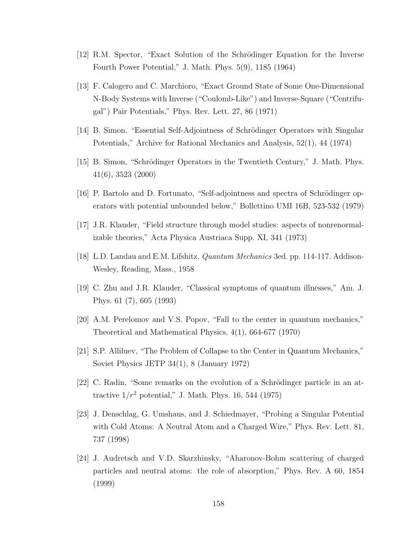
[12] R.M. Spector, “Exact Solution of the Schrodinger Equation for the Inverse
Fourth Power Potential,” J. Math. Phys. 5(9), 1185 (1964)
[13] F. Calogero and C. Marchioro, “Exact Ground State of Some One-Dimensional
N-Body Systems with Inverse (“Coulomb-Like”) and Inverse-Square (“Centrifu-
gal”) Pair Potentials,” Phys. Rev. Lett. 27, 86 (1971)
[14] B. Simon, “Essential Self-Adjointness of Schrodinger Operators with Singular
Potentials,” Archive for Rational Mechanics and Analysis, 52(1), 44 (1974)
[15] B. Simon, “Schrodinger Operators in the Twentieth Century,” J. Math. Phys.
41(6), 3523 (2000)
[16] P. Bartolo and D. Fortunato, “Self-adjointness and spectra of Schrodinger op-
erators with potential unbounded below,” Bollettino UMI 16B, 523-532 (1979)
[17] J.R. Klauder, “Field structure through model studies: aspects of nonrenormal-
izable theories,” Acta Physica Austriaca Supp. XI, 341 (1973)
[18] L.D. Landau and E.M. Lifshitz, Quantum Mechanics 3ed. pp. 114-117. Addison-
Wesley, Reading, Mass., 1958
[19] C. Zhu and J.R. Klauder, “Classical symptoms of quantum illnesses,” Am. J.
Phys. 61 (7), 605 (1993)
[20] A.M. Perelomov and V.S. Popov, “Fall to the center in quantum mechanics,”
Theoretical and Mathematical Physics, 4(1), 664-677 (1970)
[21] S.P. Alliluev, “The Problem of Collapse to the Center in Quantum Mechanics,”
Soviet Physics JETP 34(1), 8 (January 1972)
[22] C. Radin, “Some remarks on the evolution of a Schrodinger particle in an at-
tractive 1/r2 potential,” J. Math. Phys. 16, 544 (1975)
[23] J. Denschlag, G. Umshaus, and J. Schiedmayer, “Probing a Singular Potential
with Cold Atoms: A Neutral Atom and a Charged Wire,” Phys. Rev. Lett. 81,
737 (1998)
[24] J. Audretsch and V.D. Skarzhinsky, “Aharonov-Bohm scattering of charged
particles and neutral atoms: the role of absorption,” Phys. Rev. A 60, 1854
(1999)
158
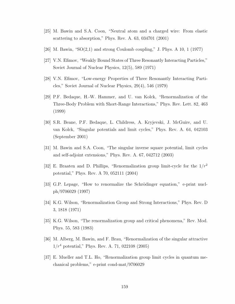
[25] M. Bawin and S.A. Coon, “Neutral atom and a charged wire: From elastic
scattering to absorption,” Phys. Rev. A. 63, 034701 (2001)
[26] M. Bawin, “SO(2,1) and strong Coulomb coupling,” J. Phys. A 10, 1 (1977)
[27] V.N. Efimov, “Weakly Bound States of Three Resonantly Interacting Particles,”
Soviet Journal of Nuclear Physics, 12(5), 589 (1971)
[28] V.N. Efimov, “Low-energy Properties of Three Resonantly Interacting Parti-
cles,” Soviet Journal of Nuclear Physics, 29(4), 546 (1979)
[29] P.F. Bedaque, H.-W. Hammer, and U. van Kolck, “Renormalization of the
Three-Body Problem with Short-Range Interactions,” Phys. Rev. Lett. 82, 463
(1999)
[30] S.R. Beane, P.F. Bedaque, L. Childress, A. Kryjevski, J. McGuire, and U.
van Kolck, “Singular potentials and limit cycles,” Phys. Rev. A. 64, 042103
(September 2001)
[31] M. Bawin and S.A. Coon, “The singular inverse square potential, limit cycles
and self-adjoint extensions,” Phys. Rev. A. 67, 042712 (2003)
[32] E. Braaten and D. Phillips, “Renormalization group limit-cycle for the 1/r2
potential,” Phys. Rev. A 70, 052111 (2004)
[33] G.P. Lepage, “How to renormalize the Schrodinger equation,” e-print nucl-
ph/9706029 (1997)
[34] K.G. Wilson, “Renormalization Group and Strong Interactions,” Phys. Rev. D
3, 1818 (1971)
[35] K.G. Wilson, “The renormalization group and critical phenomena,” Rev. Mod.
Phys. 55, 583 (1983)
[36] M. Alberg, M. Bawin, and F. Brau, “Renormalization of the singular attractive
1/r4 potential,” Phys. Rev. A. 71, 022108 (2005)
[37] E. Mueller and T.L. Ho, “Renormalization group limit cycles in quantum me-
chanical problems,” e-print cond-mat/9706029
159
[38] E.B. Kolomeisky and J.P. Straley, “Universality classes for line-depinning tran-
sitions,” Phys. Rev. B 46, 12664 (1992)
[39] T. Kraemer et al, “Evidence for Efimov quantum states in an ultracold gas of
caesium atoms,” Nature 440, 315 (2006)
[40] E. Braaten and H.-W. Hammer, “Universality in Few-Body Systems with Large
Scattering Length,” e-print cond-mat/0410417 (2006)
[41] R. Jackiw, “Delta function potentials in two- and three-dimensional quantum
mechanics,” in M.A.B. Beg Memorial Volume, ed. A. Ali and P. Hoodbhoy.
World Scientific, Singapore, 1991
[42] D. Birmingham, K.S. Gupta, and S. Sen, “Near-horizon conformal structure of
black holes,” Phys. Lett. B 505, 191 (2001)
[43] H. Camblong and C. Ordonez, “Renormalization in conformal quantum me-
chanics,” hep-th/0305035 (2005)
[44] H. Camblong and C. Ordonez, “Anomaly in conformal quantum mechanics:
from molecular physics to black holes,” Phys. Rev. D. 68, 125013 (2003)
[45] H. Camblong, L.N. Epele, H. Fanchiotti, and C.A. Garcia Canal, “Renormal-
ization of the Inverse Square Potential,” Phys. Rev. Lett. 85(8), 1590 (2000)
[46] S.A. Coon and B. Holstein, “Anomalies in quantum mechanics: the 1/r2 po-
tential,” Am. J. Phys 70 (5), 513 (2002)
[47] H. Camblong, L.N. Epele, H. Fanchiotti, and C.A. Garcia Canal, “Dimensional
transmutation and dimensional regularization in quantum mechanics, I. General
Theory,” e-print hep-th/0003255 (2001)
[48] H. Camblong, L.N. Epele, H. Fanchiotti, and C.A. Garcia Canal, “Dimensional
transmutation and dimensional regularization in quantum mechanics, II. Rota-
tional Invariance,” Ann. Phys. 287, 57-100 (2001)
[49] A. Das and S. Pernice, “Supersymmetry and singular potentials,” Nucl. Phys.
B 561, 357 (1999)
[50] A. Jevicki and J.P. Rodrigues, “Singular potentials and supersymmetry break-
ing,” Phys. Lett. B 146, 55 (1984)
160

[51] A. Essin and D.J. Griffiths, “Quantum Mechanics of the 1/x2 potential,” Am.
J. Phys. 74(2), February 2006
[52] K.S. Gupta and S.G. Rajeev, “Renormalization in quantum mechanics,” Phys.
Rev. D. 48, 5940 (1993)
[53] Paul Davies and David Betts, Quantum Mechanics. CRC, 1994
[54] John S. Townsend, A Modern Approach to Quantum Mechanics. Univ Science
Books; Sausalito, CA; 2000
[55] L.R. Mead and J. Godines, “An analytical example of renormalization in two-
dimensional quantum mechanics,” Am. J. Phys 59(10), 935 (1991)
[56] George Arfken and Hans J. Weber, Mathematical Methods for Physicists. Har-
court/Academic Press, San Diego, 2001
[57] G.N. Watson, A Treatise on the Theory of Bessel Functions. University Press,
Cambridge , 1944
[58] Milton Abramowitz and Irene Stegun (ed.), Handbook of Mathematical Func-
tions with Formulas, Graphs, and Mathematical Tables. US Govt. Print Office,
Washington, 1964
[59] I.R. Lapidus, “Scattering by two-dimensional circular barrier, hard circle, and
delta function ring potentials,” Am. J. Phys. 53, 269 (1985)
[60] I.R. Lapidus, “Quantum-mechanical scattering in two dimensions,” Am. J.
Phys. 50, 45 (1982)
[61] Leonard I. Schiff, Quantum Mechanics. McGraw-Hill, New York, 1968
[62] Roger G. Newton, Scattering Theory of Waves and Particles. McGraw-Hill,
New York, 1966
[63] C. Manuel and R. Tarrach, “Perturbative Renormalization in Quantum Me-
chanics,” e-print hep-th/9309013 (1993)
[64] P. Gosdzinsky and R. Tarrach, “Learning quantum field theory from elementary
quantum mechanics,” Am. J. Phys. 59(1), 70 (1991)
161
[65] B. Holstein, “Anomalies for Pedestrians,” Am. J. Phys. 61, 142 (1993)
[66] A. Cabo, et al, “On Scale Invariance and Anomalies in Quantum Mechanics,”
Am. J. Phys. 66, 240 (1998)
[67] S.-L. Nyeo, “Regularization methods for delta-function potentials in two-
dimensional quantum mechanics,” Am. J. Phys. 68(6), 571 (2000)
[68] D. Phillips, S.R. Beane, and T.D. Cohen, “Nonperturbative regularization and
renormalization: simple examples from nonrelativistic quantum mechanics,”
Ann. Phys. 263, 255 (1998)
[69] M.A. Naimark, Linear Differential Operators Volume 2. F. Ungar Pub Co., New
York, 1967
[70] Eberhard Zeidler, Applied Functional Analysis: Applications to Mathematical
Physics. Springer, New York, 1996
[71] John B. Conway, A Course in Functional Analysis. Springer, New York, 1985
[72] Tosio Kato, Perturbation Theory for Linear Operators. Springer, New York,
1966
[73] Jurgen Jost, Postmodern Analysis. Springer, New York, 1998
[74] S. Albeverio, F. Gesztesy, R. Hoegh-Kroen, H. Holden, Solvable Models in
Quantum Mechanics. AMS, Providence, 1988
[75] Michael Reed and Barry Simon, Methods of Modern Mathematical Physics Vol.
2: Fourier analysis, Self-Adjointness. Academic Press, New York, 1972
[76] V. Araujo, F.A.B. Coutinho, and J. Fernando Perez, “Operator domains and
self-adjoint operators.” Am. J. Phys. 72 (2), 203 (2004)
[77] G. Bonneau, J. Faraut, and G. Valent, “Self-adjoint extensions of operators and
the teaching of quantum mechanics,” Am. J. Phys. 69 (3), 322 (2001)
[78] T.F. Jordan, “Conditions on wave functions derived from operator domains,”
Am. J. Phys. 44 (6), 567 (1976)
[79] Leslie E. Ballentine, Quantum Mechanics. World Scientific, Singapore, 1998
162
[80] M. Carreau, E. Farhi, S. Gutmann, and P.F. Mende, “The Functional Integral
for Quantum Systems with Hamiltonians Unbounded from Below,” Ann. Phys.
204, 186-207 (1990)
[81] B. Kayser, “Classical Limit of Scattering in a 1/r2 Potential,” Am. J. Phys. 42,
960 (November 1974)
[82] Stephen T. Thornton and Jerry B. Marion, Classical Dynamics of Particles and
Systems, 5ed. Brooks/Cole; Belmont, CA; 2004
[83] R. de la Madrid Modino, Quantum Mechanics in Rigged Hilbert Space Language.
Ph.D. Thesis, Universidad de Valladolid, 2001
[84] M. Klaus, “On the Bound State of Schrodinger Operators in One Dimension,”
Ann. Phys. 108, 288 (1977)
[85] B. Simon, “The Bound State of Weakly Coupled Schrodinger Operators in One
and Two Dimensions,” Ann. Phys., 97, 279 (1976)
[86] C. Schwartz, “Almost Singular Potentials,” J. Math. Phys. 17(6), 863 (1976)
[87] R. Delbourgo and V.B. Prasad, “Dimensional continuation for bound state
problems,” J. Phys. A 10(1), 105 (1977)
[88] M. Bawin, “Schwartz’s Method and Goldstein’s Eigenvalue Problem,” J. Phys.
A 10(11), 1977
[89] A.K. Grant and J. Rosner, “Classical orbits in power-law potentials,” Am. J.
Phys. 62(4), 310 (1994)
[90] L. Mittag and M.J. Stephen, “Conformal transformations and the application of
complex variables in mechanics and quantum mechanics,” Am. J. Phys. 60(3),
March 1992
[91] F. Cooper, A. Khare, and U. Sukhatme, “Supersymmetry and quantum me-
chanics,” Physics Reports 251(5-6), 267-385 (1995)
[92] H. Falomir and P.A.G. Pisani, “Self-adjoint extensions and SUSY breaking in
supersymmetric quantum mechanics,” J. Phys. A 38, 4665-4683 (2005)
163
[93] H. Falomir, M.A. Muschietti, and P.A.G. Pisani, “On the resolvent and spectral
functions of a second-order differential operator with a regular singularity,” J.
Math. Phys. 45, 4560 (2004)
[94] B.D. Esry, C.H. Greene, and J.P. Burke Jr., “Recombination of Three Atoms
in the Ultracold Limit,” Phys. Rev. Lett. 83, 1751-1754 (1999)
[95] I. Tsutsui, T. Fulop, and T. Cheon, “Connection conditions and the spectral
family under singular potentials,” J. Phys. A 36, 275 (2003)
[96] I. Tsutsui, T. Fulop, and T. Cheon, “Mobius structure of the spectral space of
Schrdinger operators with point interaction,” J. Math. Phys. 42, 5687 (2001)
[97] T. Cheon and T. Shigehara, “Realizing discontinuous wave functions with renor-
malized short-range potentials,” Phys. Lett. A 243, 111 (1998)
[98] R. Loudon, “One Dimensional Hydrogen Atom,” Am. J. Phys. 27, 649 (1959)
[99] L.K. Haines and D.H. Roberts, “One-Dimensional Hydrogen Atom,” Am. J.
Phys. 37, 1145 (1969)
[100] M. Andrews, “Ground State of the One-Dimensional Hydrogen Atom,” Am. J.
Phys. 34, 1194 (1966)
[101] M. Andrews, “Singular Potentials in One Dimension,” Am. J. Phys. 44, 1064
(1976)
[102] C.L. Hammer and T.A. Weber, “Comments on the One-Dimensional Hydrogen
Atom,” Am. J. Phys. 56, 281 (1988)
[103] A.N. Gordeyev and S.C. Chhajlany, “One-dimensional hydrogen atom: a sin-
gular potential in quantum mechanics,” J. Phys. A 30, 6893 (1997)
[104] V.B. Gostev, V.K. Peres-Fernandes, A.R. Frenkin, and G.A. Chizhov, “One-
Dimensional Hydrogen Atom,” Moscow University Bulletin of Physics, 44, 22
(1989)
[105] L. Lathouwers, “The Hamiltonian 12d2
dx2 + x2
2+ λ
x2 Reobserved,” J. Math. Phys.
16, 1393 (1975)
164
[106] R. Jackiw, “Dynamical Symmetry of the Magnetic Vortex,” Ann. Phys. 201, 83
(1990)
[107] V. de Alfaro, S. Fubini, and G. Furlan, Nuovo Cimento A 34, 569 (1976)
[108] F.D.M. Haldane, “Exact Jastrow-Gutzwiller resonating-valence-bond ground
state of the spin-1/2 antiferromagnetic Heisenberg chain with 1/r2 exchange,”
Phys. Rev. Lett. 60, 635 (1988)
[109] B. Sriram Shastry, “Exact solution of an S = 1/2 Heisenberg antiferromagnetic
chain with long-ranged interactions,” Phys. Rev. Lett. 60, 639 (1988)
[110] Y. Yu, “Calogero-Sutherland gas of ultracold Bose atoms,” e-print cond-
mat/0603340 (2006)
165