selection of homogeneous samples 1 the effect of...

Selection of Homogeneous Samples 1

The Effect of Selection of Samples for Homogeneity on Type I Error Rate

Donald W. Zimmerman

Carleton University

Key words: statistical significance test, Student t test, Welch t test, separate-variances t test,

significance level, Type I error, homogeneity of variance, conditional probability

Send correspondence to: Donald W. Zimmerman 1978 134A Street Surrey, B.C. V4A 6B6 Canada Phone: (604) 531-9313 Fax: (604) 531-2092 E-mail: [email protected]


Abstract

Type I Error Probabilities of Statistical Tests Increased

by Selection of Homogeneous Samples

Donald W. Zimmerman

Carleton University

The Type I error probability of the two-sample Student t test is known to deviate from the

statistical significance level when variances are unequal and, at the same time, sample sizes are

unequal. The present simulation study indicates that, for various sample sizes and ratios of

population standard deviations, the conditional probability of a Type I error, under the condition

that the ratio of sample standard deviations falls in a narrow interval close to 1.00, is larger than

the unconditional probability of a Type I error. This result emphasizes that it is essential to

distinguish between homogeneity of population variances and homogeneity of sample variances.

If population variances are heterogeneous and sample sizes are unequal, a Student t test will be

invalid, whether or not sample variances of treatment groups happen to be equal. Accordingly, it

is not possible for researchers to protect the significance level of the test by explicit selection of

homogeneous samples.


Type I Error Probabilities of Statistical Tests Increased

by Selection of Homogeneous Samples

Donald W. Zimmerman

Carleton University

It is well known that parametric tests of location, such as the Student t test and the

ANOVA F test, depend on an assumption of homogeneity of variances in treatment groups.

Violation of the assumption substantially modifies statistical significance levels, especially when

sample sizes are unequal. When a larger variance is associated with a smaller sample size, the

probability of a Type I error exceeds the significance level, and when a larger variance is

associated with a larger sample size, the probability of a Type I error falls below the significance

level (Hsu, 1938; Overall, Atlas, and Gibson, 1995; Scheffe', 1959; Zimmerman, 1996). There is

considerable evidence that separate-variances versions of the t test effectively restore the

significance level under these conditions. Tests with good properties have been introduced by

Alexander and Govern (1994), Hsuing, Olejnik, and Huberty (1994), Satterthwaite (1946), Welch

(1938, 1947), and Wilcox, Charlin, & Thompson (1986).

It is generally agreed that preliminary tests of homogeneity of variance have not been

successful in data analysis (see, for example, Hays, 1988, p. 303). If the choice of a test of

location depends on a preliminary test of equality of variances, it is still possible for the

significance level to be severely distorted even if the test chosen as a substitute performs well.

For example, in previous simulation studies (Overall, Atlas, and Gibson, 1995; Zimmerman,

1996a; Zimmerman and Zumbo, 1993), the Welch separate-variances t test turned out to be quite

effective for a wide range sample sizes and ratios of population variances.

However, a two-stage procedure that included a preliminary test of equality of variances

was ineffective (Zimmerman, 1996b). That is, when substitution of a separate-variances test for

the Student t test in the second stage was conditional on rejection of the null hypothesis of equal


variances in the first stage, the significance level was substantially altered. The bias under the

compound procedure was accounted for by Type II errors of the preliminary test. These results

suggest that the best practical solution to the problem of heterogeneous variances is unconditional

substitution of a separate-variances t test for the Student t test whenever sample sizes are unequal.

The present paper explores a different approach to these issues. It does not attempt to

find a preliminary test that can detect unequal population variances, enabling an appropriate test

to be substituted for the t test. Rather, it asks the question: If population variances initially are

heterogeneous, and if it is possible to find samples having equal or nearly equal variances, how is

the Type I error probability of a t test modified? In other words, this study investigates the

conditional probability of a Type I error under violation of homogeneity of variance, the

condition being that sample variances are equal. This equality may come about as a chance result

of random sampling or through explicit selection in a research study.

Computer Simulation Method

Normal deviates were generated by the method of Box and Muller (1958), based on the

transformations 12

1 2( 2 log ) cos(2 )X U Uπ= − and 12

1 2( 2 log ) sin(2 ),Y U Uπ= − where U1 and

U2 are pseudorandom numbers on the interval (0,1). As a check, normal deviates also were

generated by the rejection method of Marsaglia and Bray (1964). The random number generator

used in the study, introduced by Marsaglia, Zaman, and Tsang (1990), has been described by

Pashley (1993, pp. 395-415). Also, random numbers were obtained from the PowerBASIC code

used in compiling the programs, and differences between these methods turned out to be

insignificant. For further information concerning generation of normal deviates see, for example,

Chambers (1977) and Morgan (1984).

Each replication of the sampling procedure obtained two independent samples of n1 and

n2 values. In successive replications, all scores in one sample were multiplied by a constant, so

that the ratio σ1/σ2 would have a predetermined value. A two-sample Student t test was then


performed on each pair of samples, and the result was evaluated at the .01, .05, and .10

significance levels.

Next, a selection method based on the ratio of sample standard deviations, s1/s2, was

introduced. If the ratio of the larger to the smaller sample standard deviation exceeded a

designated value, such as 1.1 or 1.5, the two samples were discarded and sampling was resumed.

This procedure was continued until 20,000 acceptable pairs had been obtained. Sometimes it was

necessary to discard more than 300,000 pairs. Finally, Student t tests were performed on all the

discarded pairs, as well as on the more homogeneous pairs resulting from selection. In this way, it

was possible to determine both the unconditional probability of a Type I error and the conditional

probability under the condition that the ratio s1/s2 falls in an interval close to 1.0.

In some parts of the study, the ratio of population standard deviations, σ1/σ2, varied

between 1.00 and 2.75 in increments of .25. In other cases, this ratio varied between 1 and 1.5 in

increments of .1. The ratio of sample sizes, n1/n2, was .2, .25, .5, 1, 2, or 5. There were 20,000

replications of the sampling procedure for each condition in the study, except in the case of the

frequency distributions in Table 4, where there were 100,000 replications.

Results of Simulations

Figures 1 and 2 show the conditional probabilities of rejecting H0 by the Student

t test as a function of the ratio of population standard deviations, σ1/σ2, for normally

------------------------------------------------------------------------

Insert Figures 1 and 2 about here

------------------------------------------------------------------------

distributed populations and for significance levels of .01, .05, and .10. Sample sizes were n1 = 10

and n2 = 40, so that the smaller sample size was associated with the larger standard deviation.

The lower curves in all three section are consistent with well known findings. That is, the

probability of a Type I error is an increasing function of the ratio of population standard


deviations under these conditions, and, for the larger values of the ratio, the probability increases

far above the nominal significance level. The upper curves in each section correspond to the

selection procedure in which the ratio of sample variances is restricted. Under this procedure,

whenever the ratio of standard deviations of a pair of samples exceeded 1.5, that pair was

eliminated and sampling was resumed. The unexpected outcome of this selection procedure is

that, over the entire range of population ratios, the conditional probability of a Type I error is

greater than the unconditional probability. Furthermore, the difference between the conditional

and unconditional probability is an increasing function of the ratio.

In Figure 2, the sample sizes and ratios were the same, but selection was more stringent:

Only sample ratios that did not exceed 1.1 were retained. Nevertheless, the conclusions are

essentially the same. In fact, the increase in the conditional probability under the more stringent

selection procedure is greater than before.

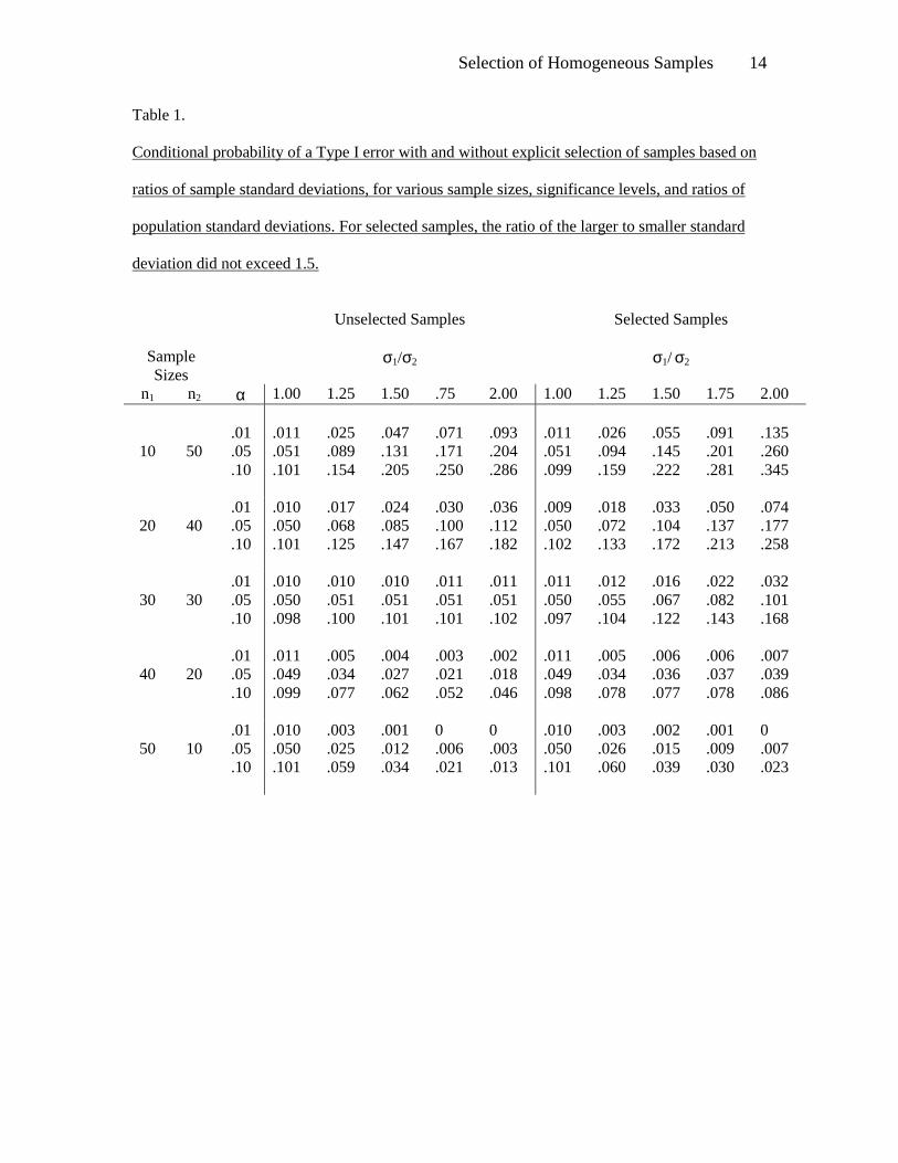
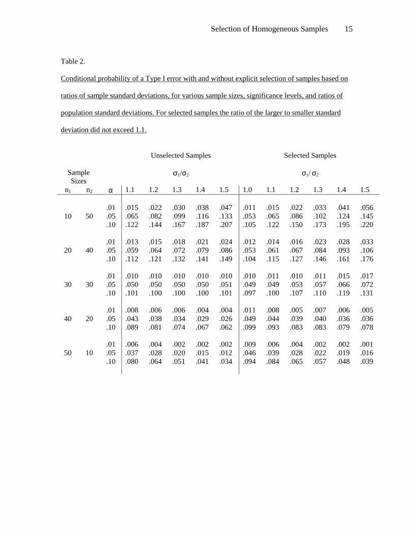
Tables 1 and 2 present similar findings for a variety of sample sizes and for ratios of

population standard deviations ranging from 1.00 to 2.00 in increments of .25. In

-----------------------------------------------------------------------

Insert Tables 1 and 2 about here

-----------------------------------------------------------------------

Table 1, sample ratios exceeding 1.5 were eliminated, and in Table 2 ratios exceeding 1.1 were

eliminated. In cases where the smaller sample size was associated with the larger standard

deviations, the results were similar to those shown in Figures 1 and 2. In cases where the larger

sample size was associated with the larger standard deviation, the unconditional probability

initially was below the significance level, consistent with known results. In this case, under the

selection procedure, the unconditional probability of a Type I error increased slightly and

remained below the nominal significance level. When sample sizes were equal, the conditional

probability increased, while the unconditional probability remained fairly constant. The

conclusions are essentially the same for all three significance levels.


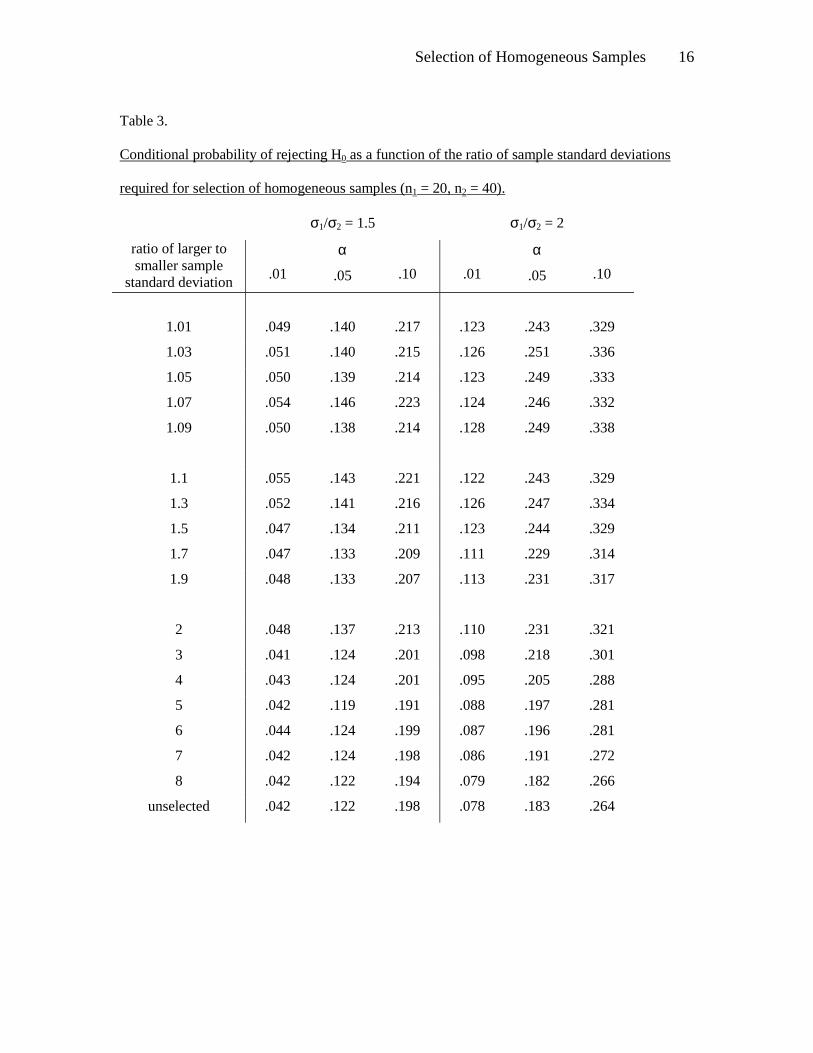
Table 3 shows results of selection based on various sample ratios. Evidently, the

conditional probability of a Type I error does not change greatly as the ratio varies

over a considerable range; ratios of 1.01, 1.1, 1.09, and 1.5 have about the same effects.

As the ratio becomes larger, there is a gradual decline in the conditional probabilities until they

are almost equal to the unconditional probabilities. The conclusions are the

--------------------------------------------------------------------

Insert Table 3 about here

--------------------------------------------------------------------

same for ratios of population standard deviations of 1.5 and 2.

Discussion

It should be emphasized that the selection procedure in the present study is not intended

to represent the sequence of events that occurs in significance testing in practice. Researchers do

not repeatedly draw samples until a desired ratio of variances is obtained. Rather, the repeated

sampling procedure in the simulations is simply a device for obtaining an estimate of the

conditional probability of a Type I error. In practical research, this probability is relevant to a

single rejection of heterogeneous samples based on inspection of sample data.

If the probability of a Type I error deviates from the nominal significance level because

population variances are unequal, then the conditional probability of a Type I error, under the

condition that sample variances are equal or nearly equal, still deviates from the significance

level, often to a greater extent. This result implies that, if population variances are unequal, then

any attempt to protect the significance level by selection of homogeneous samples from those

populations is futile.

Formally stated, let V = sX /sY, where sX and sY are standard deviations of samples from

populations with standard deviations σX and σY. Let t be the two-sample Student t statistic and tC

its critical value for testing H0: µX − µY = 0. Then,


[ ]1/ ,C CP t t a V a P t t > < < > >

where 1 < a < V. That is, the conditional probability of rejecting H0, under the condition that the

ratio of the larger to the smaller sample standard deviations is bounded by a designated value, a,

is larger than the unconditional probability of rejecting H0. Of course, the present simulations do

not prove this inequality.

The unconditional probability is known to be an increasing function of the ratio of

population standard deviations when the larger standard deviation is associated with the smaller

sample size and a decreasing function of this ratio when the reverse is true (Hsu, 1938, Scheffé,

1959). The present simulation data appears to indicate that the conditional probability, despite

explicit selection, is an increasing function of this ratio. Furthermore, the difference between the

conditional and unconditional probabilities, in both cases, is an increasing function of the same

ratio.

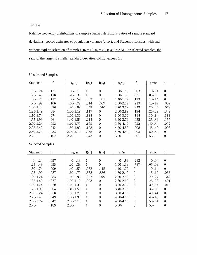
An explanation of these results is suggested by the data in Table 4, which includes

relative frequency distributions of standard deviations of two samples based on

------------------------------------------------------------------------

Insert Table 4 about here

------------------------------------------------------------------------

100,000 replications. The table also presents distributions of ratios of sample standard deviations

and distributions of the error term in the denominator of the t statistic,

2 21 1 2 2

1 2 1 2

( 1) ( 1) 1 1 ,2

n s n sn n n n

− + − + + −

for both selected and unselected samples. In this case, n1 =10, n2 = 40, and σ1/σ2 = 2.5. If the

ratio of the larger to the smaller standard deviation exceeded 1.2, the pair was eliminated.

Evidently, the selection procedure not only made the samples more homogeneous as

intended, it also reduced the size of the error term and spuriously increased the magnitude of the t


statistic. This effect counteracted any improvement resulting from more homogeneous samples.

The diminished error term is explained by the fact that a decrease in the variability of scores

through resampling is more probable than an increase. As a kind of “regression,” it is more likely

for extreme values to be replaced by less deviant ones than for additional extreme values to

appear through resampling.

It should be emphasized that resampling of this type is not typical of experimentation and

data analysis in practical research. Investigators do not as a rule continue sampling until equal

sample variances are found. The purpose of the simulation procedure in the present paper was to

obtain an estimate of the conditional probability of a Type I error under the condition that s1 = s2

when σ1 ≠ σ2.

For practical purposes, this finding is relevant to violation of homogeneity of variance in

a research study, whether or not repeated sampling occurs. In many studies, investigators do not

know in advance whether or not the population variances associated with treatment groups are

homogeneous, and they usually suspend judgment until two or more samples are obtained.

Suppose that the unknown population variances are decidedly unequal. If by chance a pair of

samples happen to have nearly equal variances, a researcher could mistakenly believe that the

homogeneity assumption is satisfied.

More likely, however, if population variances are unequal, pairs of samples will have

unequal variances. At one time, a common practice was to substitute a nonparametric method for

a parametric test of location, but, as noted above, this procedure is ineffective. A less common

practice is to reject or modify the samples by further selection of subjects until the variances are

approximately equal.

The present results reveal that neither strategy overcomes the distortion of the

significance level of the t test and that selection makes the situation worse. The homogeneity

assumption refers strictly to population variances, not sample variances. If the assumption is not

satisfied, obtaining more homogeneous samples, either by chance or by explicit selection, does


not restore the desired significance level. This remains true even if a stringent criterion of

homogeneity is adopted and the ratio of sample standard deviations is required to fall in an

extremely narrow interval close to 1.0.

Not only are preliminary tests of equality of variances unproductive, but also the entire

quest for homogeneous samples in research is likely to be misguided. Instead of basing decisions

about assumptions on sample data, investigators should be concerned with whether or not the

homogeneity assumption is reasonable in the light of what is known about populations. Of course,

in many cases, the characteristics of populations are unknown. This fact emphasizes once again

that the best practical strategy in significance testing is unconditional substitution of a separate-

variances version of the t test for the Student t test whenever sample sizes are unequal.

The present results also have some implications for meta-analysis, as well as for

individual studies. Because of general acceptance of the assumption of homogeneity of variance,

researchers may avoid or abandon projects when available samples obviously have unequal

variances. Or, they may retain samples having equal variances without paying sufficient attention

to the characteristics of populations. The entire collection of reported research studies designed to

assess differences between groups may include a disproportionate number employing invalid

statistical tests.


References

Alexander, R.A., & Govern, D.M. (1994). A new and simpler approximation for

ANOVA under variance heterogeneity. Journal of Educational and Behavioral Statistics, 19, 91-

101.

Box, G.E.P., & Muller, M. (1958). A note on the generation of normal deviates. Annals

of Mathematical Statistics, 29, 610-611.

Chambers, J.M. (1977). Computational methods for data analysis. New York: Wiley.

Hays, W.L. (1988). Statistics (4th ed.). New York: Holt, Rinehart, & Winston.

Hsu, P.L. (1938). Contributions to the theory of Student’s t test as applied to the problem

of two samples. Statistical Research Memoirs, 2, 1-24.

Hsuing, T.H., Olejnik, S.F., & Huberty, C.J. (1994). Comment on a Wilcox test statistic

for comparing means when variances are unequal.

Marsaglia, G., & Bray, T.A. (1964). A convenient method for generating normal

variables. SIAM Review, 6, 260-264.

Marsaglia, G., Zaman, A., & Tsang, W.W. (1990). Toward a universal random number

generator. Statistics & Probability Letters, 8, 35-39.

Morgan, B.J.T. (1984). Elements of simulation. London: Chapman & Hall.

Overall, J.E., Atlas, R.S., & Gibson, J.M. (1995). Tests that are robust against variance

heterogeneity in k ´ 2 designs with unequal cell frequencies. Psychological Reports, 76, 1011-

1017.

Pashley, P.J. (1993). On generating random sequences. In G. Keren & C. Lewis (Eds.) A

handbook for data analysis in the behavioral sciences: Methodological issues (pp. 395-415).

Hillsdale, NJ: Lawrence Erlbaum Associates.

Satterthwaite, F.E. (1946). An approximate distribution of estimates of variance

components. Biometrics Bulletin, 2, 110-114.


Scheffé, H. (1959). The analysis of variance. New York: Wiley.

Welch, B.L. (1938). The significance of the difference between two means when the

population variances are unequal. Biometrika, 29, 350-362.

Welch, B.L. (1947). The generalization of Student’s problem when several different

population variances are involved. Biometrika, 34, 29-35.

Wilcox, R.R., Charlin, V.L., & Thompson, K.L. (1986). Monte Carlo results on the

robustness of the ANOVA, F, W, and F* statistics. Communications in Statistics: Simulation and

Computation, 15, 933-943.

Zimmerman, D.W. (1996a). A note on homogeneity of variance of scores and ranks.

Journal of Experimental Education, 64, 351-362.

Zimmerman, D.W. (1996b). Some properties of preliminary tests of equality of variances

in the two-sample location problem. Journal of General Psychology, 123,

217-231.

Zimmerman, D.W., & Zumbo, B.D. (1993). Rank transformations and the power of the

Student t test and the Welch t' test for non-normal populations with unequal variances. Canadian

Journal of Experimental Psychology, 47, 523-539.


Author Notes

The computer program was written in PowerBASIC, version 3.2, PowerBASIC, Inc.,

Carmel, CA. A listing of the program can be obtained by writing to Donald W. Zimmerman, 1978

134A Street, Surrey, B.C., Canada, V4A 6B6.

Email: [email protected]


Table 1.

Conditional probability of a Type I error with and without explicit selection of samples based on

ratios of sample standard deviations, for various sample sizes, significance levels, and ratios of

population standard deviations. For selected samples, the ratio of the larger to smaller standard

deviation did not exceed 1.5.

Unselected Samples

Selected Samples

Sample Sizes

σ1/σ2 σ1/ σ2

n1 n2 α 1.00 1.25 1.50 .75 2.00 1.00 1.25 1.50 1.75 2.00

10

50

.01 .05 .10

.011 .051 .101

.025 .089 .154

.047 .131 .205

.071 .171 .250

.093 .204 .286

.011 .051 .099

.026 .094 .159

.055 .145 .222

.091 .201 .281

.135 .260 .345

20

40

.01

.05

.10

.010

.050

.101

.017

.068

.125

.024

.085

.147

.030

.100

.167

.036

.112

.182

.009

.050

.102

.018

.072

.133

.033

.104

.172

.050

.137

.213

.074

.177

.258

30

30

.01

.05

.10

.010

.050

.098

.010

.051

.100

.010

.051

.101

.011

.051

.101

.011

.051

.102

.011

.050

.097

.012

.055

.104

.016

.067

.122

.022

.082

.143

.032

.101

.168

40

20

.01

.05

.10

.011

.049

.099

.005

.034

.077

.004

.027

.062

.003

.021

.052

.002

.018

.046

.011

.049

.098

.005

.034

.078

.006

.036

.077

.006

.037

.078

.007

.039

.086

50

10

.01

.05

.10

.010

.050

.101

.003

.025

.059

.001

.012

.034

0 .006 .021

0 .003 .013

.010

.050

.101

.003

.026

.060

.002

.015

.039

.001

.009

.030

0 .007 .023


Table 2. Conditional probability of a Type I error with and without explicit selection of samples based on

ratios of sample standard deviations, for various sample sizes, significance levels, and ratios of

population standard deviations. For selected samples the ratio of the larger to smaller standard

deviation did not exceed 1.1.

Unselected Samples

Selected Samples

Sample Sizes

σ1/σ2 σ1/ σ2

n1 n2 α 1.1 1.2 1.3 1.4 1.5 1.0 1.1 1.2 1.3 1.4 1.5

10

50

.01 .05 .10

.015 .065 .122

.022 .082 .144

.030 .099 .167

.038 .116 .187

.047 .133 .207

.011 .053 .105

.015 .065 .122

.022 .086 .150

.033 .102 .173

.041 .124 .195

.056 .145 .220

20

40

.01

.05

.10

.013

.059

.112

.015

.064

.121

.018

.072

.132

.021

.079

.141

.024

.086

.149

.012

.053

.104

.014

.061

.115

.016

.067

.127

.023

.084

.146

.028

.093

.161

.033

.106

.176

30

30

.01

.05

.10

.010

.050

.101

.010

.050

.100

.010

.050

.100

.010

.050

.100

.010

.051

.101

.010

.049

.097

.011

.049

.100

.010

.053

.107

.011

.057

.110

.015

.066

.119

.017

.072

.131

40

20

.01

.05

.10

.008

.043

.089

.006

.038

.081

.006

.034

.074

.004

.029

.067

.004

.026

.062

.011

.049

.099

.008

.044

.093

.005

.039

.083

.007

.040

.083

.006

.036

.079

.005

.036

.078

50

10

.01

.05

.10

.006

.037

.080

.004

.028

.064

.002

.020

.051

.002

.015

.041

.002

.012

.034

.009

.046

.094

.006

.039

.084

.004

.028

.065

.002

.022

.057

.002

.019

.048

.001

.016

.039


Table 3. Conditional probability of rejecting H0 as a function of the ratio of sample standard deviations

required for selection of homogeneous samples (n1 = 20, n2 = 40).

σ1/σ2 = 1.5 σ1/σ2 = 2

ratio of larger to smaller sample

standard deviation

.01 α

.05

.10

.01 α

.05

.10

1.01

.049

.140

.217

.123

.243

.329

1.03 .051 .140 .215 .126 .251 .336

1.05 .050 .139 .214 .123 .249 .333

1.07 .054 .146 .223 .124 .246 .332

1.09

.050 .138 .214 .128 .249 .338

1.1 .055 .143 .221 .122 .243 .329

1.3 .052 .141 .216 .126 .247 .334

1.5 .047 .134 .211 .123 .244 .329

1.7 .047 .133 .209 .111 .229 .314

1.9

.048 .133 .207 .113 .231 .317

2 .048 .137 .213 .110 .231 .321

3 .041 .124 .201 .098 .218 .301

4 .043 .124 .201 .095 .205 .288

5 .042 .119 .191 .088 .197 .281

6 .044 .124 .199 .087 .196 .281

7 .042 .124 .198 .086 .191 .272

8 .042 .122 .194 .079 .182 .266

unselected .042 .122 .198 .078 .183 .264


Table 4.

Relative frequency distributions of sample standard deviations, ratios of sample standard

deviations, pooled estimates of population variance (error), and Student t statistics, with and

without explicit selection of samples (n1 = 10, n2 = 40, σ1/σ2 = 2.5). For selected samples, the

ratio of the larger to smaller standard deviation did not exceed 1.2.

Unselected Samples

Student t f s1, s2 f(s1) f(s2) s1/s2 f error f 0 - .24 .25- .49 .50- .74 .75- .99 1.00-1.24 1.25-1.49 1.50-1.74 1.75-1.99 2.00-2.24 2.25-2.49 2.50-2.74 2.75-

.121 .118 .112 .106 .096 .084 .074 .061 .052 .042 .033 .102

0- .19 .20- .39 .40- .59 .60- .79 .80- .99 1.00-1.19 1.20-1.39 1.40-1.59 1.60-1.79 1.80-1.99 2.00-2.19 2.20-

0 0 .002 .014 .049 .117 .188 .214 .185 .123 .065 .043

0 0 .351 .639 .010 0 0 0 0 0 0 0

0- .99 1.00-1.39 1.40-1.79 1.80-2.19 2.20-2.59 2.60-2.99 3.00-3.39 3.40-3.79 3.80-4.19 4.20-4.59 4.60-4.99 5.00-

.003 .031 .113 .213 .242 .194 .114 .055 .023 .008 .003 .001

0-.04 .05-.09 .10-.14 .15-.19 .20-.24 .25-.29 .30-.34 .35-.39 .40-.44 .45-.49 .50-.54 .55-

0 0 0 .002 .073 .349 .383 .157 .032 .003 0 0

Selected Samples

Student t f s1, s2 f(s1) f(s2) s1/s2 f error f 0 - .24 .25- .49 .50- .74 .75- .99 1.00-1.24 1.25-1.49 1.50-1.74 1.75-1.99 2.00-2.24 2.25-2.49 2.50-2.74 2.75-

.097 .095 .090 .087 .083 .077 .070 .064 .058 .049 .042 .189

0- .19 .20- .39 .40- .59 .60- .79 .80- .99 1.00-1.19 1.20-1.39 1.40-1.59 1.60-1.79 1.80-1.99 2.00-2.19 2.20-

0 0 .082 .658 .257 .003 0 0 0 0 0 0

0 0 .115 .836 .049 0 0 0 0 0 0 0

0- .99 1.00-1.39 1.40-1.79 1.80-2.19 2.20-2.59 2.60-2.99 3.00-3.39 3.40-3.79 3.80-4.19 4.20-4.59 4.60-4.99 5.00-

.213 .787 0 0 0 0 0 0 0 0 0 0

0-.04 .05-.09 .10-.14 .15-.19 .20-.24 .25-.29 .30-.34 .35-.39 .40-.44 .45-.49 .50-.54 .55-

0 0 0 .033 .548 .401 .018 0 0 0 0 0


Figure Captions

Figure 1.

Conditional probability of rejecting H0 by the Student t test as a function of the ratio of

population standard deviations for unselected pairs of samples and for pairs in which the ratio of

the larger to the smaller standard deviation did not exceed 1.5.

Figure 2.

Conditional probability of rejecting H0 by the Student t test as a function of the ratio of

population standard deviations for unselected pairs of samples and for pairs in which the ratio of

the larger to the smaller standard deviation did not exceed 1.1


α α α α = .01

σσσσ1111/σ/σ/σ/σ2222

1.00 1.25 1.50 1.75 2.00 2.25 2.50 2.75

Cond

ition

al P

roba

bilit

y

of

Rej

ectin

g H

0

0.00

0.05

0.10

0.15

0.20

0.25

α α α α = .05


1.00 1.25 1.50 1.75 2.00 2.25 2.50 2.75

Cond

ition

al P

roba

bilit

y

of

Rej

ectin

g H

0

0.00

0.05

0.10

0.15

0.20

0.25

0.30

0.35

α α α α = .10


1.00 1.25 1.50 1.75 2.00 2.25 2.50 2.75

Cond

ition

al P

roba

bilit

y

of

Rej

ectin

g H

0

0.00

0.050.10

0.150.200.25

0.300.350.40

0.45

unselected samplesselected samples




αααα = .01

σσσσ1111/σσσσ2222

1.0 1.1 1.2 1.3 1.4 1.5 1.6 1.7

Cond

ition

al P

roba

bilit

y

of R

ejec

ting

H0

0.00

0.01

0.02

0.03

0.04

0.05

0.06

0.07

0.08

0.09

αααα = .05


1.0 1.1 1.2 1.3 1.4 1.5 1.6 1.7

Cond

ition

al P

roba

bilit

y

of R

ejec

ting

H0

0.00

0.05

0.10

0.15

0.20

α α α α = .10


1.0 1.1 1.2 1.3 1.4 1.5 1.6 1.7

Cond

ition

al P

roba

bilit

y

of R

ejec

ting

H0

0.00

0.05

0.10

0.15

0.20

0.25

0.30




selection of homogeneous samples 1 the effect of...

Documents