Selection Biases: Truncation and Censoring

Jogesh Babu

Penn State University

Outline

1 Censoring vs Truncation

2 Censoring

3 Statistical inferences for censoring

4 Truncation

5 Statistical inferences for truncation

6 Doubly truncated data

7 Recent methods

Censoring vs Truncation

Censoring: Sources/events can be detected, but thevalues (measurements) are not known completely. Weonly know that the value is less than some number.

Truncation: An object can be detected only if its value isgreater than some number; and the value is completelyknown in the case of detection. For example, objects ofcertain type in a specific region of the sky will not bedetected by the instrument if the apparent luminosity ofobjects is less than a certain lower limit. This oftenhappens due to instrumental limitations or due to ourposition in the universe.

The main difference between censoring and truncation isthat censored object is detectable while the object is noteven detectable in the case of truncation.

Example: Left/Right Censoring

Right Censoring: the exact value X is not measurable,but only T = min(X,C) and δ = I(X ≤ C) areobserved.

Left Censoring: Only T = max(X,C) and δ = I(X ≥ C)are observed.

Example: Interval/Double Censoring

This occurs when we do not observe the exact time of failure,but rather two time points between which the event occurred:

(T, δ) =

(X, 1) : L < X < R(R, 0) : X > R

(L,−1) : X < L

where L and R are left and right censoring variables.

Survival Function

Cumulative failure function:

F (t) = P (X ≤ t)

Survivor function:

S(t) = P (X > t) = 1− F (t)

Kaplan-Meier Estimator

Nonparametric estimate of survivor function S(t)

Intuitive graphical presentation

Commonly used to compare two populations

Kaplan-Meier Estimator (continued)

Let

ti: ith ordered observation

di: number of ‘censored’ events at ith ordered observation

Ri: number of subjects ‘at-risk’ at ith ordered observation

The Kaplan Meier estimator of the survival function is

S(t) =∏ti≤t

(1− di

Ri

)

Truncation

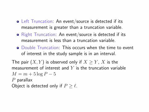
Left Truncation: An event/source is detected if itsmeasurement is greater than a truncation variable.

Right Truncation: An event/source is detected if itsmeasurement is less than a truncation variable.

Double Truncation: This occurs when the time to eventof interest in the study sample is in an interval.

The pair (X, Y ) is observed only if X ≥ Y , X is themeasurement of interest and Y is the truncation variableM = m+ 5 logP − 5P parallaxObject is detected only if P ≥ `.

Forty years ago, astrophysicist Donald Lynden-Bell (1971,MNRAS.155, 95) derived a fundamental statistical resultin the appendix to an astronomical study: the uniquenonparametric maximum likelihood estimator for aunivariate dataset subject to random truncation.

The method is needed to establish luminosity functionsfrom flux-limited surveys, and is far better than the morepopular heuristic 1/Vmax method by Schmidt (1968).

Schafer (2007) gives a nonparametric estimation forestimating the bivariate distribution when one variable istruncated.

Kelly et al. use a Bayesian approach for a normal mixturemodel (combination of Gaussians) to the luminosityfunction.

Lynden-Bell Estimator

Lynden-Bell-Woodroofe Estimator

Model: observe y only if y > u(x).

Data: (x1, y1), . . . , (xn, yn).

Risk set numbers:

Nj = #{i : ui ≤ y(j) and yi ≤ y(j)}

where ui = u(xi) and y(i) is ith ordered value ofy = (y1, . . . , yn)

In the KM estimator, Nj is the number of points at riskjust before the jth event.

The only differences in comparable points betweentruncated cases and censoring cases is that points withyi > yk but t(xi) > yk are not considered at risk in thetruncated case. This is because these points cannot beobserved.

Lynden-Bell- Woodroofe Estimator (continued)

Lyden-Bell-Woodroofe survival function estimator:

LBW (t) =∏

y(j)≤t

(1− 1

Nj

)

Lynden-Bell, D. 1971, MNRAS, 155, 95Woodroofe, M. 1985, Ann. Stat., 13, 163

Doubly truncated data:

Efron’s Nonparametric MLE

15,343 quasars – 22 –

0 1 2 3 4 5

−24

−26

−28

−30

Redshift

Abs

olut

e M

agni

tude

Fig. 1.— Quasar data from the Sloan Digital Sky Survey, the sample from Richards et al.

(2006). Quasars within the dashed region are used in this analysis. The removed quasars

are those with M ≤ −23.075, which fall into the irregularly-shaped corner at the lower left

of the plot, and those with z ≤ 3 and apparent magnitude greater than 19.1, which fall into

a very sparsely sampled region.

Data

The data shown in the figure, consists of 15,343 quasars.

From these, any quasar is removed if it hasz ≥ 5.3, z ≤ 0.1,M ≥ −23.075, or M ≤ −30.7.

In addition, for quasars of redshift less than 3.0, onlythose with apparent magnitude between 15.0 and 19.1,inclusive, are kept; for quasars of redshift greater than orequal to 3.0, only those with apparent magnitude between15.0 and 20.2 are retained.

These boundaries combine to create the irregular shapeshown by the dashed line.

This truncation removes two groups of quasars from theRichards et al. (2006) sample. There are 15,057 quasarsremaining after this truncation.

References

Efron, B. and Petrosian, V. 1992 ApJ, 399, 345.

Efron, B. and Petrosian, V. 1999 JASA, 94, 447.

Schafer, C. M. (2007, ApJ, 661, 703) uses semi-parametricmethods log φ(z,M) = f(z) + g(M) + h(z,M.θ),(zi,Mi) observed.

Kelly et al. (2008, ApJ, 682, 874) use Bayesian approachfor normal mixture model.

The results obtained are better than the heuristic 1/Vmax

of Schmidt (1968, ApJ, 151, 393)