selecting the optimal method to calculate daily global ... · earth syst. sci., 16, 983–1000, ......

Hydrol. Earth Syst. Sci., 16, 983–1000, 2012www.hydrol-earth-syst-sci.net/16/983/2012/doi:10.5194/hess-16-983-2012© Author(s) 2012. CC Attribution 3.0 License.

Hydrology andEarth System

Sciences

Selecting the optimal method to calculate daily global referencepotential evaporation from CFSR reanalysis data for application ina hydrological model study

F. C. Sperna Weiland1,2, C. Tisseuil3, H. H. Durr 1, M. Vrac4, and L. P. H. van Beek1

1Department of Physical Geography, Utrecht University, P.O. Box 80115, 3508 TC, Utrecht, The Netherlands2Deltares, P.O. Box 177, 2600 MH, Delft, The Netherlands3Museum National d’Histoire Naturelle, UMR BOREA-IRD 207/CNRS 7208/MNHN/UPMC,Departement Milieux et Peuplements Aquatiques, Paris, France4Laboratoire des Sciences du Climat et de l’Environnement (LSCE-IPSL) CNRS/CEA/UVSQ, Centre d’etude de Saclay,Orme des Merisiers, 91191 Gif-sur-Yvette Cedex, France

Correspondence to:F. C. Sperna Weiland ([email protected])

Received: 1 July 2011 – Published in Hydrol. Earth Syst. Sci. Discuss.: 28 July 2011Revised: 15 March 2012 – Accepted: 16 March 2012 – Published: 27 March 2012

Abstract. Potential evaporation (PET) is one of the maininputs of hydrological models. Yet, there is limited consen-sus on which PET equation is most applicable in hydrolog-ical climate impact assessments. In this study six differentmethods to derive global scale reference PET daily time se-ries from Climate Forecast System Reanalysis (CFSR) dataare compared: Penman-Monteith, Priestley-Taylor and origi-nal and re-calibrated versions of the Hargreaves and Blaney-Criddle method. The calculated PET time series are (1) eval-uated against global monthly Penman-Monteith PET time se-ries calculated from CRU data and (2) tested on their usabil-ity for modeling of global discharge cycles.

A major finding is that for part of the investigated basinsthe selection of a PET method may have only a minor in-fluence on the resulting river flow. Within the hydrologicalmodel used in this study the bias related to the PET methodtends to decrease while going from PET, AET and runoff todischarge calculations. However, the performance of indi-vidual PET methods appears to be spatially variable, whichstresses the necessity to select the most accurate and spa-tially stable PET method. The lowest root mean squareddifferences and the least significant deviations (95 % signifi-cance level) between monthly CFSR derived PET time seriesand CRU derived PET were obtained for a cell-specific re-calibrated Blaney-Criddle equation. However, results showthat this re-calibrated form is likely to be unstable underchanging climate conditions and less reliable for the calcu-lation of daily time series. Although often recommended,the Penman-Monteith equation applied to the CFSR data didnot outperform the other methods in a evaluation against PET

derived with the Penman-Monteith equation from CRU data.In arid regions (e.g. Sahara, central Australia, US deserts),the equation resulted in relatively low PET values and, con-sequently, led to relatively high discharge values for drybasins (e.g. Orange, Murray and Zambezi). Furthermore, thePenman-Monteith equation has a high data demand and theequation is sensitive to input data inaccuracy. Therefore, werecommend the re-calibrated form of the Hargreaves equa-tion which globally gave reference PET values comparableto CRU derived values for multiple climate conditions.

The resulting gridded daily PET time series providea new reference dataset that can be used for futurehydrological impact assessments in further research, ormore specifically, for the statistical downscaling of dailyPET derived from raw GCM data. The dataset can bedownloaded fromhttp://opendap.deltares.nl/thredds/dodsC/opendap/deltares/FEWS-IPCC.

1 Introduction

Climate change is likely to induce alterations in the hydro-logical cycle (IPCC, 2007 and references therein). To assessand quantify the possible changes, multiple hydrological im-pact studies have been conducted on the local, continentaland global scale, the latter being of interest in this study. Inaddition to temperature and precipitation (PR; for list of ab-breviations see Table 1), evaporation is required as input formost hydrological models used in impact studies (Kay andDavies, 2008; Oudin et al., 2005). However, both potential

Published by Copernicus Publications on behalf of the European Geosciences Union.

http://opendap.deltares.nl/thredds/dodsC/opendap/deltares/FEWS-IPCC


984 F. C. Sperna Weiland et al.: Calculating global potential evaporation from CFSR re-analysis data

and actual evapotranspiration (AET; for list of abbreviationssee Table 1) are seldomly monitored and General CirculationModel (GCM) datasets, employed for future impact assess-ments (Sperna Weiland et al., 2012b), often lack AET data(PCMDI, 2010).

Here, we prefer to calculate potential evaporation (PET)from GCM data and to derive AET within a hydrologicalmodel over using GCM AET directly. This because withinglobal hydrological models (GHMs), AET is calculated ona higher grid resolution and processes related to transpira-tion and soil moisture are modeled with a water balance in-stead of energy balance approach which at least guaranteesthat negative evaporation does not occur (Sperna Weiland etal., 2012a). In addition, GCM AET is often biased due to,amongst others, biases in PR, radiation and soil moistureavailability (Mahanama and Koster, 2005; Elshamy et al.,2009; Sperna Weiland et al., 2012a). Of course, it should benoted here that off-line calculation of PET and AET can alsobe biased by deviations in GCM radiation used as input forsome of the PET equations or through interaction betweenthe different atmospheric variables within the GCM.

Within hydrological model studies monthly PET time-series, or monthly PET time-series downscaled to daily val-ues (for example based on temperature), have frequentlybeen used (Van Beek, 2008; Sperna Weiland et al., 2010;Arnell, 2011). Currently, most hydrological models run ona daily or smaller time-step, as most hydrological processesshow a high variability over time. Consequently, these mod-els can also benefit from daily PET time-series as model in-put. In addition, the input data of PET equations is now oftenprovided on a daily time step. Therefore, this study focuseson calculation of daily PET time series using daily valuesof the required atmospheric variables. A historical globalgridded PET time series will be created that can be used asreference for the statistical downscaling of daily GCM data.Downscaling of PET time series was preferred over down-scaling of the individual GCM input variables of the PETequation, since by individual downscaling inconsistenciesbetween the atmospheric input variables can be introduced(Piani et al., 2010).

For the creation of these PET time series a consistentobservational dataset of current climatic conditions at highspatial and temporal resolution is needed. Here we usedthe recently developed Climate Forecast System Reanalysis(CFSR) dataset (Saha et al., 2006, 2010) which is of partic-ular interest for three major reasons. Firstly, it is a data setwith a high spatial (∼0.3◦

× ∼0.3◦) and temporal (6-hourly)resolution covering the entire globe. Secondly, in the shortterm, the CFSR dataset is likely to supersede its predecessor,the widely known US NCEP/NCAR (National Center for En-vironmental Prediction/National Center for Atmospheric Re-search) reanalysis data (Kalnay et al., 1996). And thirdly, theCFSR dataset contains all required atmospheric fields to cal-culate and compare a range of PET equations.

Table 1. Abbreviations.

Abbreviaton Long name/description

AET Actual evapotranspirationBC Blaney-CriddleBCorig Original Blaney-Criddle equationBCrecal Re-calibrated Blaney-Criddle equationCDF Cumulative distribution functionCFSR Climate forecast system reanalysisCFSR PET Potential evaporation calculated from CFSR dataCFSR PM PET Penman-Monteith potential evaporation from CFSR dataCRU Climate research unit, University of East AngliaCRU TS 2.1 1901–96 Monthly Grids of Terrestrial Surface Climate, CRUCRU CL 1.0 1961-90 mean monthly terrestrial climatology, CRUCRU PET Potential evaporation calculated from CRU dataCRU PM PET Penman-Monteith potential evaporation from CRU dataCV Coefficient of variationDJF December, January, FebruaryFAO United Nations Food and Agriculture OrganizationGCM General circulation model / global climate modelGHM Global hydrological modelGLCC Global Land Cover CharacterizationGRDC Global runoff data centreHG Hargreaves equationHGorig Original Hargreaves equationHGrecal Re-calibrated Hargreaves equationHGPET Hargreaves potential evaporationJJA June, July, AugustMAM March, April, MayNCAR National Center for Atmospheric ResearchNCEP National Centre for Environmental PredictionPCR-GLOBWB PCRaster code global water balance modelPET Potential evaporationPM Penman-MonteithPR PrecipitationPT Priestley-TaylorQC (Channel) dischargeQL Cell specific runoffRMSD Root mean squared differenceSON September, October, NovemberUS United States

Limited consensus exists on which PET equation is mostapplicable in global hydrological impact studies. Severalstudies illustrated that the selected method can actually deter-mine the direction of projected change in future water avail-ability (Boorman, 2010; Kingston et al., 2009; Arnell, 1999).Therefore, we here analyze six well documented equations ofdifferent complexity: the physical-based Penman-Monteithequation (PM), the empirical Hargreaves (HG), Priestley-Taylor (PT) and Blaney-Criddle (BC) equations and modifiedversions of the Hargreaves (HGrecal) and Blaney-Criddle(BCrecal) equations. The PM equation is generally consid-ered as the standard (Hargreaves et al., 2003; Droogers andAllen, 2002; Gavilan et al., 2006) as its physically based na-ture is preferred over simpler empirical equations (Kay andDavies, 2008; Arnell, 1999; Kingston et al., 2009). However,due to its high input data requirement the PM may be sensi-tive to biases in mulptiple GCM and re-analysis atmosphericvariables (Oudin et al., 2005). The HG equation is a simpli-fied alternative for the PM equation (Hargreaves and Samani,1985; Hargreaves et al., 2003). Here the influence of hu-midity is approximated with the diurnal temperature range.

Hydrol. Earth Syst. Sci., 16, 983–1000, 2012 www.hydrol-earth-syst-sci.net/16/983/2012/

F. C. Sperna Weiland et al.: Calculating global potential evaporation from CFSR re-analysis data 985

The equation is applicable in a variety of climatic condi-tions and shows overall good agreement with the PM method(Droogers and Allen, 2002). Several studies highlighted sig-nificant improvement of the HG equation by increasing itsmultiplication factor (Droogers and Allen, 2002). This willbe tested here as well.

The more empirical BC equation depends on less inputvariables and may therefore be less sensitive to GCM and re-analysis data quality (Kingston et al., 2009; Weiß and Men-zel, 2008; Lu et al., 2005). With the temperature-based BCequation the computation time required for both calculationof PET and downscaling of the required input variables canbe reduced, while the method provides results comparable toother PET methods (Oudin et al., 2005; Blaney and Criddle,1950). Yet, Jensen (1966) showed that the climate depen-dency of the BC equation disables its application in multipledifferent climate zones. To overcome this problem we testedthe local-recalibrated BC method proposed by Ekstrom etal. (2007).

The main goal of this study is the construction of a globalgridded dataset of reference PET at high spatial (0.5 degree)and temporal (daily) resolution from CFSR reanalysis datausing one of the following six PET equations; PM, HG, PT,BC and the HGrecal and BCrecal equations. The constructeddaily PET dataset will be validated annually and seasonallyfor the period 1979–2002 against the Climate Research Unit(CRU) dataset (CRU TS 2.1 and CRU CL 1.0) which is oftenconsidered as a standard (Mitchell and Jones, 2005; New etal., 2000, 1999; Droogers and Allen, 2002; IPCC, 2007). Ina first step, a sensitivity analysis of the influence of the differ-ences between individual CFSR and CRU atmospheric vari-ables on calculated PET is given. In a final step, the transferof differences between the six PET methods throughout thehydrological modeling chain (i.e. from PET to AET to runoffand discharge) will be assessed by inter-method comparisonand the goodness-of-fit between modeled and observed riverdischarge.

2 Data and methods

2.1 CFSR reanalysis data

The CFSR dataset is a reanalysis product which is developedas part of the Climate Forecast System (Saha et al., 2006,2010) at the National Centers for Environmental Prediction(NCEP). The CFSR dataset became available in 2010 and su-persedes the previous NCEP/NCAR reanalysis dataset whichhas been widely used in downscaling studies (e.g. Michelan-geli et al., 2009; Maurer et al., 2010; Wilby et al., 1998). Atthis stage the CFSR dataset spans the period 1979 to presentand has a resolution of approximately 0.25 degrees aroundthe equator to 0.5 degrees beyond the tropics (Higgins et al.,2010). In this study, 6-hourly temperature, radiation, airpressure and wind data were averaged to a daily time-step for

the period 1979–2002. These daily time series were then in-terpolated to the regular 0.5 degrees PCR-GLOBWB modelgrid using bilinear interpolation.

2.2 CRU reference potential evaporation

For validation reference historical PET time series werecalculated from the CRU datasets with the by the UnitedNations Food and Agriculture Organization (FAO) recom-mended PM equation (Monteith, 1965; Allen et al., 1998).Temperature, vapor pressure and cloud cover were retrievedfrom the CRU TS2.1 monthly time series (New et al., 2000).Wind speed was obtained from the monthly climatology,CRU CL 1.0 (New et al., 1999) because monthly CRU TS2.1time series are not provided for this variable. Diffusiv-ity, i.e. the effectiveness by which heat and vapour can beexchanged with the atmosphere, was calculated followingAllen et al. (1998). As radiation is not included in the CRUdatasets, a standard climatological maximum radiation cyclewas calculated using the day-number and latitude as input(Allen et al., 1998). This maximum radiation was reduced toincoming radiation at the surface with monthly CRU cloudcover time-series. The resulting monthly PET time series,which are here used as reference for the validation of theCFSR derived PET, are subject to uncertainties as well dueto biases in and availability of the meteorological input dataand due to simplifications in the equation. Yet, to our opin-ion they form one of the best available global reference PETdataset (Mitchell and Jones, 2005; Droogers and Allen, 2002;IPCC, 2007). For application in the hydrological model theCRU time-series have been downscaled to daily values usingthe monthly PR and temperature quantities from the CRUdatasets and the daily distribution of these variables from theCFSR dataset following Van Beek et al. (2008). It shouldbe noted that the measurement based CRU dataset is sub-ject to inaccuracies as well. In addition, the data from theCRU CL 1.0 climatology is derived from data for the period1961 to1990 and has been used for the calculation of PET forthe period 1990 to 2002 as well. This may have introducedinconsistencies due to meteorological changes over the pastdecades. The influence of these inconsistencies is minimizedby analyzing long-term average PET results only.

2.3 Potential evaporation equations

Within this study we compare daily CFSR PET time seriesderived with six different PET equations. The equationsconsidered are: (1) the physically based PM equation, (2)the radiation and temperature-based PT equation, (3) the HGequation which requires as input time-varying temperatureand extra-terrestrial radiation, (4) the empirical temperature-based BC equation and additional modified forms of the (5)HG and (6) BC equations (Table 2).

The BC equation was applied in its original form (BCorig)and in a re-calibrated form (BCrecal) following Ekstrom et

www.hydrol-earth-syst-sci.net/16/983/2012/ Hydrol. Earth Syst. Sci., 16, 983–1000, 2012


Table 2. Potential evaporation equations.

Method Acronym Equation Reference

Penman-Monteith PM ET0 =1(Rn−G)+ρacp

(es−ea )ra

λv1+γ (1+rsra

)Monteith (1965)

Hargreaves HGorig ET0 = 0.0023·Ra ·(T +17.8) ·TR0.50 Hargreaves and Samani (1985)Modified Hargreaves HGrecal ET0 = 0.0031·Ra ·(T +17.8) ·TR0.50 This studyPriestley-Taylor PT ET0 =α 1Rn

λv(1+γ )Priestley and Taylor (1972)

Blaney-Criddle BCorig ET0 =p(0.46T +8) Blaney and Criddle (1950)recalibrated Blaney-Criddle BCrecal ET0 =p(aT +b) Ekstrom et al. (2007)

λv = latent heat of vaporization (J /g), 1 = the slope of the saturation vapour pressure temperature relationship (Pa K−1), Rn = net radiation (W m−2), G = Soil heat flux (W m−2),cp = specific heat of the air (J kg−1 K−1), ρa = mean air density at constant pressure (kg m−3), es − ea = vapor pressure deficit (Pa),rs = surface resistances (m s−1), ra = aerodynamic

resistances (m s−1), γ = psychrometric constant (66 Pa K−1), Ra = extraterrestrial radiation (MJ m−2 day−1), T = mean daily temperature (◦C), TR = temperature range (◦C),α = empirical multiplier (–; 1.26),p = mean daily percentage of annual daytime hours (%),a and b are the coefficients of the Blaney-Criddle equation which are adjusted tocell specific values in the recalibration.

al. (2007). In this modified BC equation, the multiplica-tive and additive coefficients (e.g. 0.46 and 8) have been re-calibrated to cell-specific values (see the resulting coefficientvalues in Fig. 1). This was done by linearly regressing thecell specific long-term average mean monthly CFSR temper-ature to the CRU derived long-term average monthly PET forthe complete period with overlapping data available for thetwo datasets (1979–2002). The slopes and intercepts of thislinear regression exercise were used to calculate the coeffi-cient values. For the empirical BC equation, which consid-ers only limited meteorological variables, a cell specific re-calibration was preferred (this is also illustrated by the largespatial variation in bias between BC PET derived from CFSRdata and reference PM PET derived from CRU data, as willbe presented in the results section).

The HG equation was also applied in its original form(HGorig) and in a re-calibrated form (HGrecal). The HGequation is recognized as an efficient empirical equation withlow input data demand, while it integrates consistent infor-mation on the spatial variability of climate conditions suchas the daily temperature range and a spatial radiation pattern.The spatial radiation pattern is defined as a fixed annual cyclewith a daily time-step where values vary with latitude and ju-lian day number (Allen, 1998). Preliminary results indicatedthat the PET time series derived from the CFSR dataset us-ing the original HG (HGorig) equation gave an overall globalunderestimation of CRU PET (as will be shown in the resultssection) with little spatial variability. Therefore, instead ofa cell-specific re-calibration, we applied a global uniformmodification to the HG equation, by increasing uniformlythe multiplication factor in the equation for all grid cellsfrom 0.0023 to 0.0031. Similar increases were proposed byAllen (1993) and Droogers and Allen (2002). To determinethe optimal value of the multiplication factor the long termaverage monthly CFSR HGorig time series were linearly fit-ted against CRU PET. The multiplication factor was then var-ied with intervals of 0.0001 until the lowest global average

a.

b.

Fig. 1. Cell specific values of the coefficients in the re-calibratedBlaney-Criddle equation. The values in(a) replace the number 0.46and the values in(b) replace the number 8 in the original Blaney-Criddle equation (ET0 =p(0.46T + 8)).

root mean squared difference (RMSD) value was obtainedfor the monthly average PET time series.

2.4 Global hydrological modelling

The global water balance was modelled with the GHM PCR-GLOBWB. For a detailed description and validation of themodel, see Van Beek et al. (2011), Van Beek (2008) andSperna Weiland et al. (2010). It should of course be notedthat the influence of biases in PET on modeled AET, runoffand discharge also depends on the GHM used. Therefore theresults of this study can not be generalized to all hydrologicalmodels.



Each model cell, with a resolution of 0.5 degrees, consistsof two vertical soil layers and one underlying groundwaterreservoir. Sub-grid parameterization is used for the schema-tization of surface water, short and tall vegetation and forcalculation of saturated areas for surface runoff as well as in-terflow. Water enters the cell as rainfall and can be storedas canopy interception or snow. Snow is accumulated whentemperature is below 0◦C and melts when temperature ishigher. Melt water and throughfall are passed to the sur-face, where they either infiltrate in the soil or become surfacerunoff. Exchange of soil water is possible between the soiland groundwater layers in both up- and downward direction,depending on soil moisture status and groundwater storage.Total runoff consists of non-infiltrating melt water, saturationexcess surface runoff, interflow and base flow.

Time series of reference PET are prescribed to the hydro-logical model and converted to AET internally. Referencepotential evapotranspiration is converted into crop-specificpotential evapotranspiration using a crop factor (Allen et al.,1998). PCR-GLOBWB distinguishes two land cover types,short and tall vegetation, given the distinctive differences inplant height, canopy cover and root distributions. The aggre-gation of different vegetation types into two land cover typesis expedient from a computation point of view. However,by basing the parameterization of the different land covertypes on the Global Land Cover Characterization (GLCC 2;Loveland et al., 2000) database which has a resolution of30 arc seconds, much of the sub-grid variability in vegeta-tion conditions can be preserved at the 0.5 degree resolution.Also, although the imposed potential evapotranspiration iscalled crop-specific, it should be noted that this concernsboth natural and cultivated areas. To account for seasonalvariations in the crop-specific evaptranspiration, the crop fac-tor is represented by a monthly climatology that reflects thephenology and in case of cultivated surfaces, also the cropcalendar.

Crop-specific potential evapotranspiration needs to be par-titioned into two fluxes, one through the soil matrix (bare soilevaporation) and one through the roots and stomata of vege-tation (transpiration). Since vegetation stands are layered andground cover variable, a break-down on the basis of the min-imum crop factor and that of the stand as a whole is preferredover one on the basis of cover fraction. Adopting the uppervalue for the minimum crop factor (0.2, Allen et al., 1998),the potential evaporation and transpiration flux become:

ES0 = ksPET (1)

T0 = kcPET (2)

where PET is reference PET (m day−1), ks is the “crop fac-tor” used for bare soil, ES0 is potential bare soil evapora-tion (m day−1), kc is the monthly crop factor andT0 is po-tential crop specific transpiration (m day−1). The aggrega-tion of crop types to two vegetation classes on a grid with

a resolution of 0.5 degrees is a simplification of real worldvegetation and will in the end impact calculated PET fields.

Potential bare soil evaporation and plant transpiration arereduced to AET based on soil moisture conditions. As sub-grid variation in soil water storage capacity is considered,part of the surface area may be saturated (Improved ArnoScheme; Hagemann and Gates, 2003). Over this saturatedarea, potential bare soil evaporation can be sustained as longas the rate does not exceed the saturated hydraulic conductiv-ity. Similarly, over the fraction of the cell where the surfaceremains unsaturated, the rate is limited by the unsaturated hy-draulic conductivity. In the case of transpiration, no transpi-ration can occur over the saturated part due to oxygen stress,while over the unsaturated area the rate diminishes betweenfull to no transpiration from field capacity to wilting point asa result of water stress. Bare soil evaporation is capable ofexhausting soil moisture in the upper soil layer of the modelonly, whereas transpiration can draw from both layers giventhe root distribution.

For each daily time-step the water balance, and its result-ing runoff and AET fluxes, are computed for all model cells.The cell specific runoff is accumulated and routed as riverdischarge along the drainage network taken from the globalDrainage Direction Map (DDM30; Doll and Lehner, 2002)using the kinematic wave approximation of the Saint-Venantequation. Due to the coarse resolution of this large scale hy-drological model, river discharge can only reliably be calcu-lated for large river basins.

2.5 Statistical validation

The six PET time series derived from CFRS data were val-idated for the period 1979 to 2002 against monthly CRUbased PM PET time series (CRUPM) and compared witheach other, using six statistical quantities:

1. A first simple comparison was made by calculatingglobal maps with biases in long-term average annualmeans:

BIAS = PETCFSR−PETCRU (3)

where PETCFSR refers to annual average PET calcu-lated from the CFSR dataset using one of the six equa-tions (Table 2) andPETCRU refers to the annual aver-age PET calculated from the CRU datasets with the PMequation. Unfortunately, there are no reference globalgridded time series of AET available. Vorosmarty etal. (1998) apply an approximation of observed AETby subtracting observed runoff from observed PR. Yet,within their study it is already stated that this approxi-mation is only valid in areas with little water regulationor abstractions and reliable PR and discharge measure-ments. And, as was also the case for several locations intheir study, we obtained negative AET values for a num-ber of basins with this method. Therefore we concluded



that the method is not reliable when applied to the se-lected global datasets. As a consequence, the CFSRderived AET and runoff maps are only validated by acomparison between methods.

2. To illustrate the significance of the biases calculated instep one, global significance maps have been calculatedfor PET, AET and local runoff independently. Heretothe significance of the differences between annual av-erage CRU and CFSR derived time series have beenquantified with the Welch’s t-test (Welch, 1947) for asignificance level of 95 %. The Welch’s adaptation ofthe standard student’s t-test is used when the two sam-ples possibly have unequal variances.

t =XCRU−XCFSR√

s2CRU

nCRU+

s2CFSR

nCFSR

(4)

WhereXCRU is the long-term annual average PET, AETor runoff value calculated from the CRU dataset andXCFSR is the long-term annual average calculated fromthe CFSR dataset for one of the six equations,SCRUis the standard deviation CRU derived annual averagePET, AET or runoff values (for all variables 24 annualvalues over the period 1979 to 2002) andSCFSR is thestandard deviation of the 24 CFSR derived annual av-erage values,nCFSR andnCFSR are the number (24) ofannual average values for both datasets.

3. To analyze the seasonal varying character of the bi-ases, global maps with cell specific RMSD (m day−1)

of the monthly time series (Eq. 5) have been created.These maps give an indication of regional performanceon the smallest time-scale at which the validation datais available:

RMSD=

√√√√√ N∑i=1

(PETCRUi−PETCFSRi

)2

N(5)

where PETCFSR refers to the monthly PET calculatedfrom the CFSR data set, PETCRU refers to the monthlyPM-based PET calculated from the CRU dataset,i isthe month number andN is the total number of months(N = 288).

4. Global maps with long-term annual and seasonal aver-age PET, AET and runoff have been calculated to il-lustrate the differences between methods while movingthrough the hydrological model chain.

5. To quantify the variation between the six different equa-tions, cell specific values of the coefficient of variation

(CV) have been calculated from long-term average PETmaps calculated with the six different PET equations:

CV =

M∑j=1

√1K

K∑k=1

(PETk,j −PETj )2

PETj

M(6)

WherePETj is the average of PET calculated with the6 equations for the specific cellj . PETk,j is the PETcalculated for thekth equation for cellj , K is the totalnumber of equations (6),M is the total number of gridcells.

In addition, global average CV values have been calcu-lated for PET, AET, runoff and discharge and basin spe-cific CV values have been calculated from the annualaverage river discharge.

6. Performance of the different methods for the reproduc-tion of correct AET amounts is more explicitly evalu-ated by comparing long-term average modeled river dis-charge with discharge observations. To this end, annualaverage discharge is modeled with PCR-GLOBWBforced with temperature, PR and PET from the CFSRdataset for a selection of 19 large rivers (Sperna Weilandet al., 2010). For validation, observed discharge wasobtained from the Global Runoff Data Centre (GRDC;GRDC, 2007). The data was adjusted by adding an esti-mation of water use (Wada et al., 2010; Sperna Weilandet al., 2010).

3 Results

3.1 Impact of differences in individual meteorologicalvariables from the CFSR and CRU datasets onPM PET

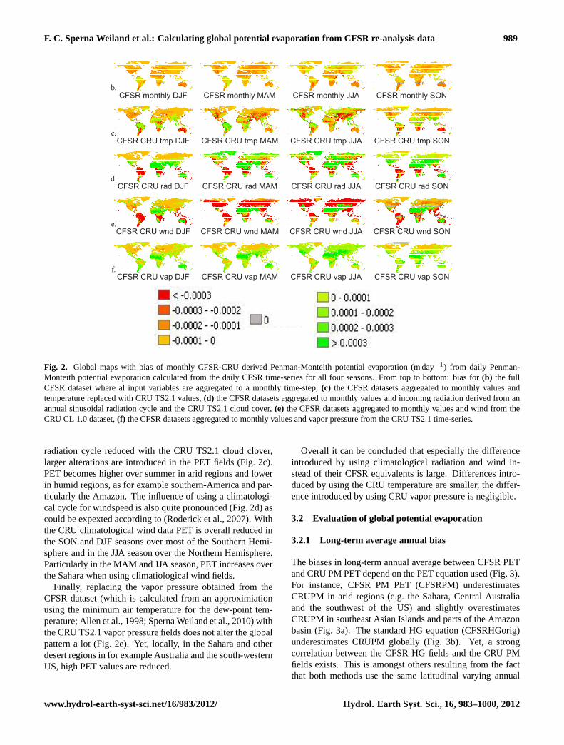
Global maps with the bias of monthly CFSR-CRU derivedPM PET from daily CFSR PM PET are shown for all fourseasons in Fig. 2. Within all these maps PET is calculatedwith the PM equation. Yet, in the top row the daily averageCFSR data is replaced by monthly averages in the calculationof PM PET. The maps show that there is limited differencein seasonal averages when using either CFSR daily or CFSRmonthly average values as input to the PM equation (Fig. 2a).Therefore, the CFSR PET time-series can be evaluated on amonthly time-scale with CRU data.

To evaluate the influence of differences in individual at-mospheric variables from the CFSR and CRU dataset, ineach row one CFSR variable is replaced with its correspond-ing CRU variable. Replacing CFSR monthly temperaturewith CRU monthly temperature does mainly introduce not-icable difference over summer in Australia, Central Asia andsouthen Australia (Fig. 2b). When replacing CFSR radia-tion with radiation derived from the daily lattitudinal varying



CFSR monthly DJF CFSR monthly MAM CFSR monthly JJA CFSR monthly SON

CFSR CRU tmp DJF CFSR CRU tmp MAM CFSR CRU tmp JJA CFSR CRU tmp SON

CFSR CRU rad DJF CFSR CRU rad MAM CFSR CRU rad JJA CFSR CRU rad SON

CFSR CRU wnd DJF CFSR CRU wnd MAM CFSR CRU wnd JJA CFSR CRU wnd SON

CFSR CRU vap DJF CFSR CRU vap MAM CFSR CRU vap JJA CFSR CRU vap SON

d.

b.

c.

e.

f.

Fig. 2. Global maps with bias of monthly CFSR-CRU derived Penman-Monteith potential evaporation (m day−1) from daily Penman-Monteith potential evaporation calculated from the daily CFSR time-series for all four seasons. From top to bottom: bias for(b) the fullCFSR dataset where al input variables are aggregated to a monthly time-step,(c) the CFSR datasets aggregated to monthly values andtemperature replaced with CRU TS2.1 values,(d) the CFSR datasets aggregated to monthly values and incoming radiation derived from anannual sinusoidal radiation cycle and the CRU TS2.1 cloud cover,(e) the CFSR datasets aggregated to monthly values and wind from theCRU CL 1.0 dataset,(f) the CFSR datasets aggregated to monthly values and vapor pressure from the CRU TS2.1 time-series.

radiation cycle reduced with the CRU TS2.1 cloud clover,larger alterations are introduced in the PET fields (Fig. 2c).PET becomes higher over summer in arid regions and lowerin humid regions, as for example southern-America and par-ticularly the Amazon. The influence of using a climatologi-cal cycle for windspeed is also quite pronounced (Fig. 2d) ascould be expexted according to (Roderick et al., 2007). Withthe CRU climatological wind data PET is overall reduced inthe SON and DJF seasons over most of the Southern Hemi-sphere and in the JJA season over the Northern Hemisphere.Particularly in the MAM and JJA season, PET increases overthe Sahara when using climatiological wind fields.

Finally, replacing the vapor pressure obtained from theCFSR dataset (which is calculated from an approximiationusing the minimum air temperature for the dew-point tem-perature; Allen et al., 1998; Sperna Weiland et al., 2010) withthe CRU TS2.1 vapor pressure fields does not alter the globalpattern a lot (Fig. 2e). Yet, locally, in the Sahara and otherdesert regions in for example Australia and the south-westernUS, high PET values are reduced.

Overall it can be concluded that especially the differenceintroduced by using climatological radiation and wind in-stead of their CFSR equivalents is large. Differences intro-duced by using the CRU temperature are smaller, the differ-ence introduced by using CRU vapor pressure is negligible.

3.2 Evaluation of global potential evaporation

3.2.1 Long-term average annual bias

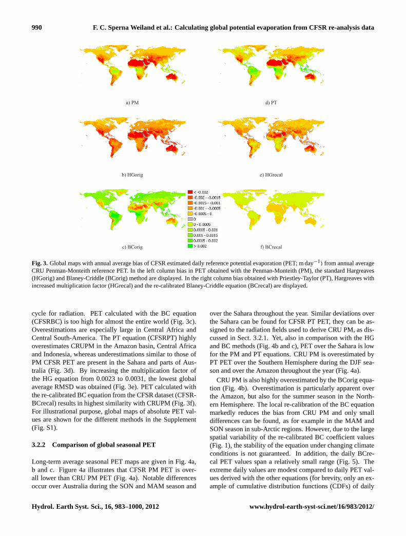
The biases in long-term annual average between CFSR PETand CRU PM PET depend on the PET equation used (Fig. 3).For instance, CFSR PM PET (CFSRPM) underestimatesCRUPM in arid regions (e.g. the Sahara, Central Australiaand the southwest of the US) and slightly overestimatesCRUPM in southeast Asian Islands and parts of the Amazonbasin (Fig. 3a). The standard HG equation (CFSRHGorig)underestimates CRUPM globally (Fig. 3b). Yet, a strongcorrelation between the CFSR HG fields and the CRU PMfields exists. This is amongst others resulting from the factthat both methods use the same latitudinal varying annual



a) PM d) PT

b) HGorig e) HGrecal

c) BCorig f) BCrecal

Fig. 3. Global maps with annual average bias of CFSR estimated daily reference potential evaporation (PET; m day−1) from annual averageCRU Penman-Monteith reference PET. In the left column bias in PET obtained with the Penman-Monteith (PM), the standard Hargreaves(HGorig) and Blaney-Criddle (BCorig) method are displayed. In the right column bias obtained with Priestley-Taylor (PT), Hargreaves withincreased multiplication factor (HGrecal) and the re-calibrated Blaney-Criddle equation (BCrecal) are displayed.

cycle for radiation. PET calculated with the BC equation(CFSRBC) is too high for almost the entire world (Fig. 3c).Overestimations are especially large in Central Africa andCentral South-America. The PT equation (CFSRPT) highlyoverestimates CRUPM in the Amazon basin, Central Africaand Indonesia, whereas underestimations similar to those ofPM CFSR PET are present in the Sahara and parts of Aus-tralia (Fig. 3d). By increasing the multiplication factor ofthe HG equation from 0.0023 to 0.0031, the lowest globalaverage RMSD was obtained (Fig. 3e). PET calculated withthe re-calibrated BC equation from the CFSR dataset (CFSR-BCrecal) results in highest similarity with CRUPM (Fig. 3f).For illustrational purpose, global maps of absolute PET val-ues are shown for the different methods in the Supplement(Fig. S1).

3.2.2 Comparison of global seasonal PET

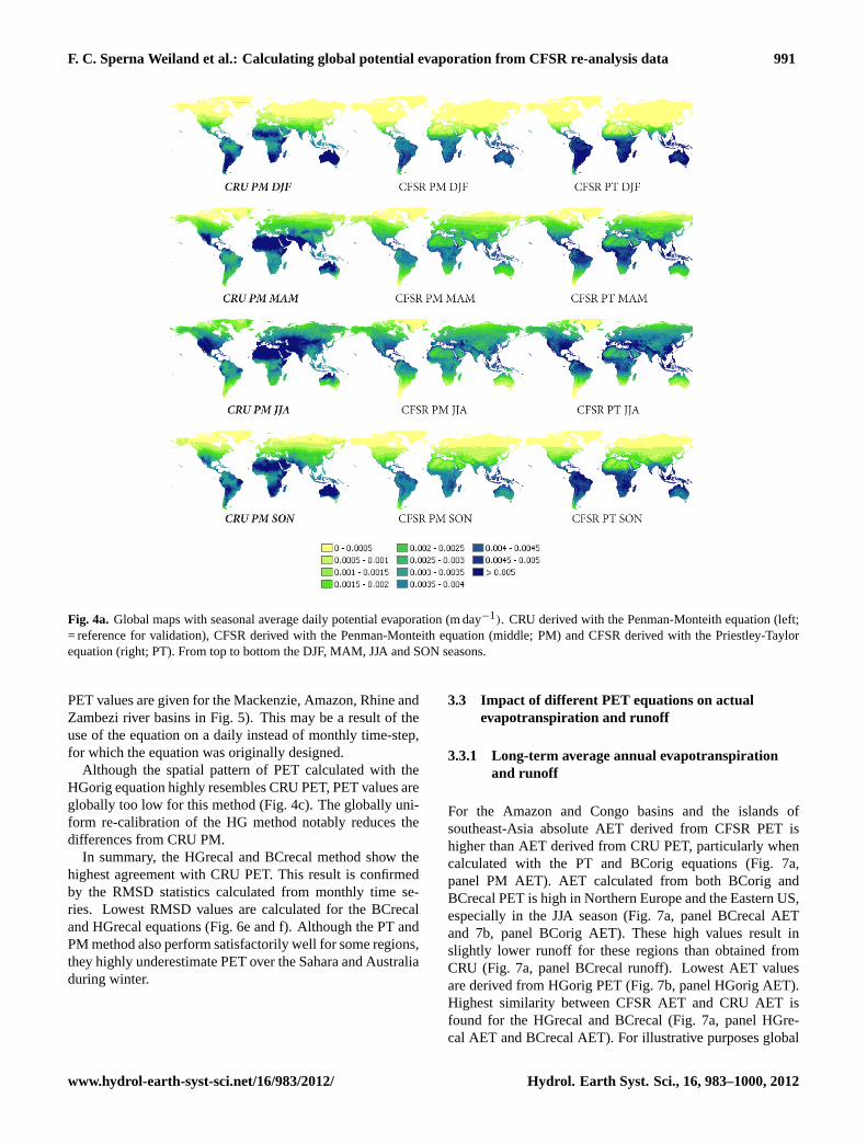
Long-term average seasonal PET maps are given in Fig. 4a,b and c. Figure 4a illustrates that CFSR PM PET is over-all lower than CRU PM PET (Fig. 4a). Notable differencesoccur over Australia during the SON and MAM season and

over the Sahara throughout the year. Similar deviations overthe Sahara can be found for CFSR PT PET, they can be as-signed to the radiation fields used to derive CRU PM, as dis-cussed in Sect. 3.2.1. Yet, also in comparison with the HGand BC methods (Fig. 4b and c), PET over the Sahara is lowfor the PM and PT equations. CRU PM is overestimated byPT PET over the Southern Hemisphere during the DJF sea-son and over the Amazon throughout the year (Fig. 4a).

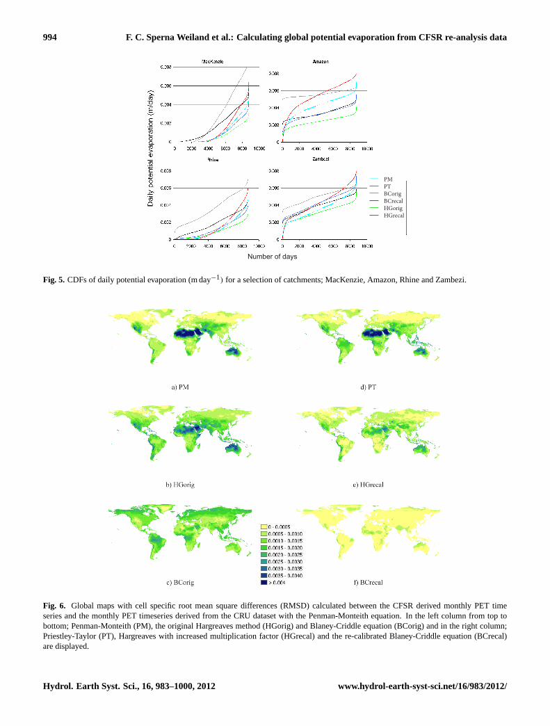
CRU PM is also highly overestimated by the BCorig equa-tion (Fig. 4b). Overestimation is particularly apparent overthe Amazon, but also for the summer season in the North-ern Hemisphere. The local re-calibration of the BC equationmarkedly reduces the bias from CRU PM and only smalldifferences can be found, as for example in the MAM andSON season in sub-Arctic regions. However, due to the largespatial variability of the re-calibrated BC coefficient values(Fig. 1), the stability of the equation under changing climateconditions is not guaranteed. In addition, the daily BCre-cal PET values span a relatively small range (Fig. 5). Theextreme daily values are modest compared to daily PET val-ues derived with the other equations (for brevity, only an ex-ample of cumulative distribution functions (CDFs) of daily



Fig. 4a. Global maps with seasonal average daily potential evaporation (m day−1). CRU derived with the Penman-Monteith equation (left;= reference for validation), CFSR derived with the Penman-Monteith equation (middle; PM) and CFSR derived with the Priestley-Taylorequation (right; PT). From top to bottom the DJF, MAM, JJA and SON seasons.

PET values are given for the Mackenzie, Amazon, Rhine andZambezi river basins in Fig. 5). This may be a result of theuse of the equation on a daily instead of monthly time-step,for which the equation was originally designed.

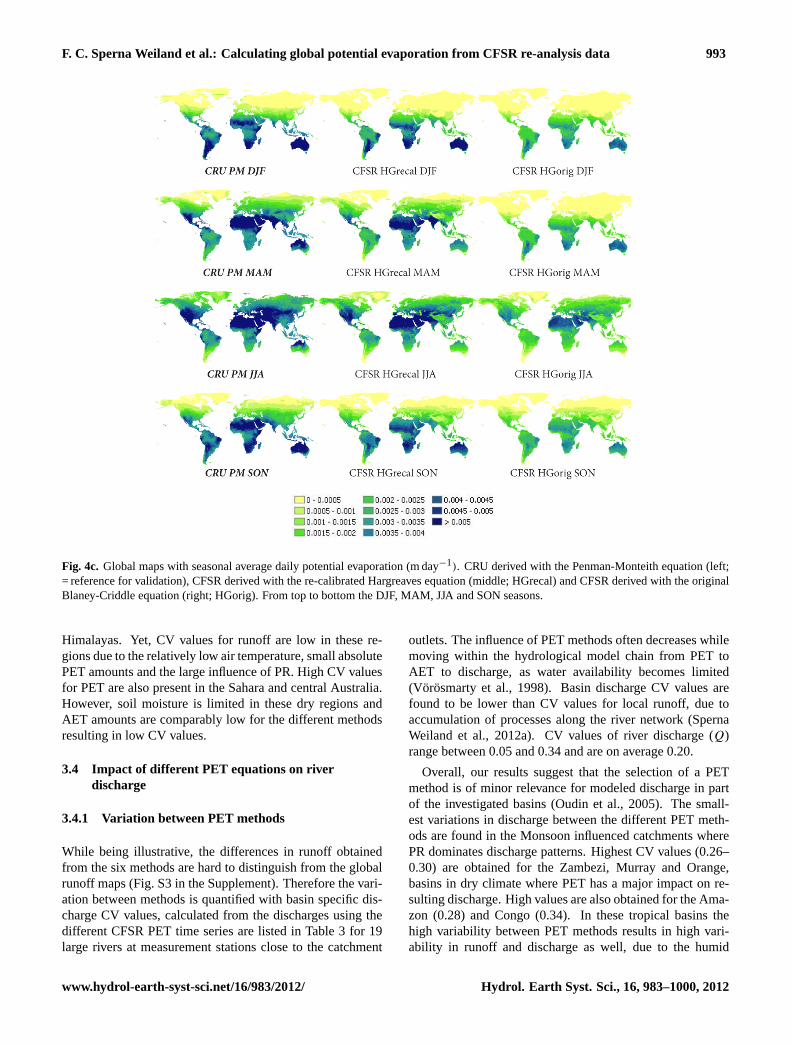
Although the spatial pattern of PET calculated with theHGorig equation highly resembles CRU PET, PET values areglobally too low for this method (Fig. 4c). The globally uni-form re-calibration of the HG method notably reduces thedifferences from CRU PM.

In summary, the HGrecal and BCrecal method show thehighest agreement with CRU PET. This result is confirmedby the RMSD statistics calculated from monthly time se-ries. Lowest RMSD values are calculated for the BCrecaland HGrecal equations (Fig. 6e and f). Although the PT andPM method also perform satisfactorily well for some regions,they highly underestimate PET over the Sahara and Australiaduring winter.

3.3 Impact of different PET equations on actualevapotranspiration and runoff

3.3.1 Long-term average annual evapotranspirationand runoff

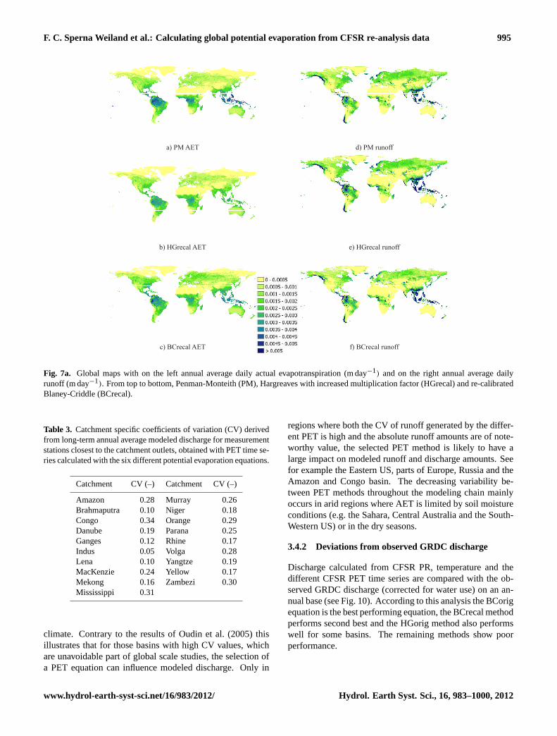
For the Amazon and Congo basins and the islands ofsoutheast-Asia absolute AET derived from CFSR PET ishigher than AET derived from CRU PET, particularly whencalculated with the PT and BCorig equations (Fig. 7a,panel PM AET). AET calculated from both BCorig andBCrecal PET is high in Northern Europe and the Eastern US,especially in the JJA season (Fig. 7a, panel BCrecal AETand 7b, panel BCorig AET). These high values result inslightly lower runoff for these regions than obtained fromCRU (Fig. 7a, panel BCrecal runoff). Lowest AET valuesare derived from HGorig PET (Fig. 7b, panel HGorig AET).Highest similarity between CFSR AET and CRU AET isfound for the HGrecal and BCrecal (Fig. 7a, panel HGre-cal AET and BCrecal AET). For illustrative purposes global



Fig. 4b. Global maps with seasonal average daily potential evaporation (m day−1). CRU derived with the Penman-Monteith equation (left;= reference for validation), CFSR derived with the re-calibrated Blaney-Criddle equation (middle; BCrecal) and CFSR derived with theoriginal Blaney-Criddle equation (right; BCorig). From top to bottom the DJF, MAM, JJA and SON seasons.

maps of seasonal AET values are given in the Supplement(Fig. S2).

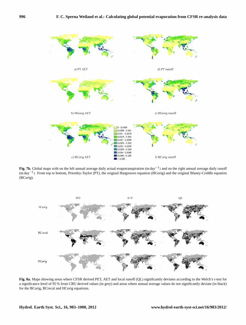
Figures 7a, b and 8 show that differences in spatial runoffpatterns are almost as small as the differences in AET pat-terns. This is a result of the fact that the runoff flux is in-fluenced by both AET and PR. Runoff is low for the PT andBCorig method (Fig. 7b, panel PT runoff and BCorig runoff).Although increasing the multiplication factor of the originalHG equation to 0.0031 resulted in higher PET values, the dif-ference in runoff derived from the two HG time series is stillsmall (Fig. 7a, panel HGrecal runoff and 7b, panel HGorigrunoff). Global seasonal runoff maps are provided for thedifferent PET equations in the Supplement (Fig. S3).

3.3.2 Variation between methods

In Fig. 8 the significance of differences (calculated with theWelch’s t-test for a significance level of 95 %) between an-nual average PET, AET and local runoff derived from CFSRdata (with any of the PET equations) and annual average

values of the same variables derived from CRU data is indi-cated. Within Fig. 8 black areas correspond to regions whereannual averages of CFSR and CRU PET derived values donot deviate significantly. Large regions without significantdeviations of CFSR PET from CRU PET only occur for theBCcal method. The BCorig and HGorig equations obviouslyresult in the largest areas with significant deviations fromCRU PET. While moving from PET to AET to local runoff(QL) the areas with significant deviations of CFSR PET fromCRU PET decrease in size as differences between the differ-ent PET methods decrease due to limited soil moisture avail-ability and the influence of PR on local runoff and discharge.

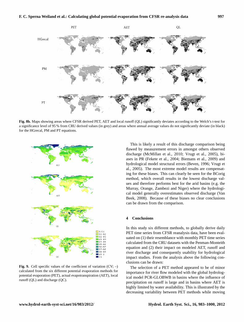
Globally the variability between the six different PETmethods also tends to decrease while moving from PET toAET and runoff, as can be seen from the cell specific CVobtained from the PET values calculated across the six dif-ferent methods (Fig. 9). For instance, the global cell aver-age CV for PET is 0.42, whereas for AET and runoff theCV values are 0.25 and 0.27 respectively. High CV valuesfor PET and AET are obtained for Northern regions and the



Fig. 4c. Global maps with seasonal average daily potential evaporation (m day−1). CRU derived with the Penman-Monteith equation (left;= reference for validation), CFSR derived with the re-calibrated Hargreaves equation (middle; HGrecal) and CFSR derived with the originalBlaney-Criddle equation (right; HGorig). From top to bottom the DJF, MAM, JJA and SON seasons.

Himalayas. Yet, CV values for runoff are low in these re-gions due to the relatively low air temperature, small absolutePET amounts and the large influence of PR. High CV valuesfor PET are also present in the Sahara and central Australia.However, soil moisture is limited in these dry regions andAET amounts are comparably low for the different methodsresulting in low CV values.

3.4 Impact of different PET equations on riverdischarge

3.4.1 Variation between PET methods

While being illustrative, the differences in runoff obtainedfrom the six methods are hard to distinguish from the globalrunoff maps (Fig. S3 in the Supplement). Therefore the vari-ation between methods is quantified with basin specific dis-charge CV values, calculated from the discharges using thedifferent CFSR PET time series are listed in Table 3 for 19large rivers at measurement stations close to the catchment

outlets. The influence of PET methods often decreases whilemoving within the hydrological model chain from PET toAET to discharge, as water availability becomes limited(Vorosmarty et al., 1998). Basin discharge CV values arefound to be lower than CV values for local runoff, due toaccumulation of processes along the river network (SpernaWeiland et al., 2012a). CV values of river discharge (Q)range between 0.05 and 0.34 and are on average 0.20.

Overall, our results suggest that the selection of a PETmethod is of minor relevance for modeled discharge in partof the investigated basins (Oudin et al., 2005). The small-est variations in discharge between the different PET meth-ods are found in the Monsoon influenced catchments wherePR dominates discharge patterns. Highest CV values (0.26–0.30) are obtained for the Zambezi, Murray and Orange,basins in dry climate where PET has a major impact on re-sulting discharge. High values are also obtained for the Ama-zon (0.28) and Congo (0.34). In these tropical basins thehigh variability between PET methods results in high vari-ability in runoff and discharge as well, due to the humid



PMPTBCorigBCrecalHGorigHGrecal

Number of days

Fig. 5. CDFs of daily potential evaporation (m day−1) for a selection of catchments; MacKenzie, Amazon, Rhine and Zambezi.

Fig. 6. Global maps with cell specific root mean square differences (RMSD) calculated between the CFSR derived monthly PET timeseries and the monthly PET timeseries derived from the CRU dataset with the Penman-Monteith equation. In the left column from top tobottom; Penman-Monteith (PM), the original Hargreaves method (HGorig) and Blaney-Criddle equation (BCorig) and in the right column;Priestley-Taylor (PT), Hargreaves with increased multiplication factor (HGrecal) and the re-calibrated Blaney-Criddle equation (BCrecal)are displayed.



a) PM AET d) PM runoff

b) HGrecal AET e) HGrecal runoff

c) BCrecal AET f) BCrecal runoff

Fig. 7a. Global maps with on the left annual average daily actual evapotranspiration (m day−1) and on the right annual average dailyrunoff (m day−1). From top to bottom, Penman-Monteith (PM), Hargreaves with increased multiplication factor (HGrecal) and re-calibratedBlaney-Criddle (BCrecal).

Table 3. Catchment specific coefficients of variation (CV) derivedfrom long-term annual average modeled discharge for measurementstations closest to the catchment outlets, obtained with PET time se-ries calculated with the six different potential evaporation equations.

Catchment CV (–) Catchment CV (–)

Amazon 0.28 Murray 0.26Brahmaputra 0.10 Niger 0.18Congo 0.34 Orange 0.29Danube 0.19 Parana 0.25Ganges 0.12 Rhine 0.17Indus 0.05 Volga 0.28Lena 0.10 Yangtze 0.19MacKenzie 0.24 Yellow 0.17Mekong 0.16 Zambezi 0.30Mississippi 0.31

climate. Contrary to the results of Oudin et al. (2005) thisillustrates that for those basins with high CV values, whichare unavoidable part of global scale studies, the selection ofa PET equation can influence modeled discharge. Only in

regions where both the CV of runoff generated by the differ-ent PET is high and the absolute runoff amounts are of note-worthy value, the selected PET method is likely to have alarge impact on modeled runoff and discharge amounts. Seefor example the Eastern US, parts of Europe, Russia and theAmazon and Congo basin. The decreasing variability be-tween PET methods throughout the modeling chain mainlyoccurs in arid regions where AET is limited by soil moistureconditions (e.g. the Sahara, Central Australia and the South-Western US) or in the dry seasons.

3.4.2 Deviations from observed GRDC discharge

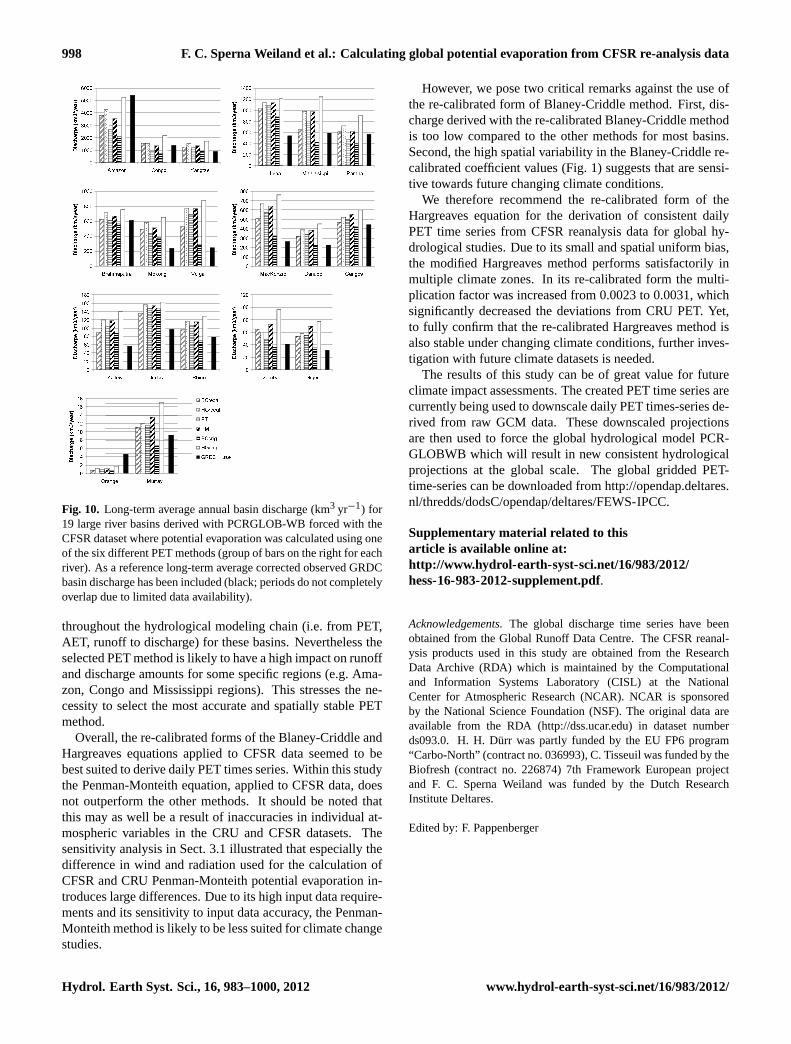
Discharge calculated from CFSR PR, temperature and thedifferent CFSR PET time series are compared with the ob-served GRDC discharge (corrected for water use) on an an-nual base (see Fig. 10). According to this analysis the BCorigequation is the best performing equation, the BCrecal methodperforms second best and the HGorig method also performswell for some basins. The remaining methods show poorperformance.



a) PT AET d) PT runoff

b) HGorig AET e) HGorig runoff

c) BCorig AET f) BCorig runoff

Fig. 7b. Global maps with on the left annual average daily actual evapotranspiration (m day−1) and on the right annual average daily runoff(m day−1). From top to bottom, Priestley-Taylor (PT), the original Hargreaves equation (HGorig) and the original Blaney-Criddle equation(BCorig).

Fig. 8a. Maps showing areas where CFSR derived PET, AET and local runoff (QL) significantly deviates according to the Welch’s t-test fora significance level of 95 % from CRU derived values (in grey) and areas where annual average values do not significantly deviate (in black)for the BCorig, BCrecal and HCorig equations.



Fig. 8b. Maps showing areas where CFSR derived PET, AET and local runoff (QL) significantly deviates according to the Welch’s t-test fora significance level of 95 % from CRU derived values (in grey) and areas where annual average values do not significantly deviate (in black)for the HGrecal, PM and PT equations.

PET

AET

QL

QC

Fig. 9. Cell specific values of the coefficient of variation (CV; –)calculated from the six different potential evaporation methods forpotential evaporation (PET), actual evapotranspiration (AET), localrunoff (QL) and discharge (QC).

This is likely a result of this discharge comparison beingflawed by measurement errors in amongst others observeddischarge (McMillan et al., 2010; Vrugt et al., 2005), bi-ases in PR (Fekete et al., 2004; Biemans et al., 2009) andhydrological model structural errors (Beven, 1996; Vrugt etal., 2005). The most extreme model results are compensat-ing for these biases. This can clearly be seen for the BCorigmethod, which overall results in the lowest discharge val-ues and therefore performs best for the arid basins (e.g. theMurray, Orange, Zambezi and Niger) where the hydrologi-cal model generally overestimates observed discharge (VanBeek, 2008). Because of these biases no clear conclusionscan be drawn from the comparison.

4 Conclusions

In this study six different methods, to globally derive dailyPET time series from CFSR reanalysis data, have been eval-uated on (1) their resemblance with monthly PET time seriescalculated from the CRU datasets with the Penman-Monteithequation and (2) their impact on modeled AET, runoff andriver discharge and consequently usability for hydrologicalimpact studies. From the analysis above the following con-clusions can be drawn:

The selection of a PET method appeared to be of minorimportance for river flow modeled with the global hydrolog-ical model PCR-GLOBWB in basins where the influence ofprecipitation on runoff is large and in basins where AET ishighly limited by water availability. This is illustrated by thedecreasing variability between PET methods while moving



Fig. 10. Long-term average annual basin discharge (km3 yr−1) for19 large river basins derived with PCRGLOB-WB forced with theCFSR dataset where potential evaporation was calculated using oneof the six different PET methods (group of bars on the right for eachriver). As a reference long-term average corrected observed GRDCbasin discharge has been included (black; periods do not completelyoverlap due to limited data availability).

throughout the hydrological modeling chain (i.e. from PET,AET, runoff to discharge) for these basins. Nevertheless theselected PET method is likely to have a high impact on runoffand discharge amounts for some specific regions (e.g. Ama-zon, Congo and Mississippi regions). This stresses the ne-cessity to select the most accurate and spatially stable PETmethod.

Overall, the re-calibrated forms of the Blaney-Criddle andHargreaves equations applied to CFSR data seemed to bebest suited to derive daily PET times series. Within this studythe Penman-Monteith equation, applied to CFSR data, doesnot outperform the other methods. It should be noted thatthis may as well be a result of inaccuracies in individual at-mospheric variables in the CRU and CFSR datasets. Thesensitivity analysis in Sect. 3.1 illustrated that especially thedifference in wind and radiation used for the calculation ofCFSR and CRU Penman-Monteith potential evaporation in-troduces large differences. Due to its high input data require-ments and its sensitivity to input data accuracy, the Penman-Monteith method is likely to be less suited for climate changestudies.

However, we pose two critical remarks against the use ofthe re-calibrated form of Blaney-Criddle method. First, dis-charge derived with the re-calibrated Blaney-Criddle methodis too low compared to the other methods for most basins.Second, the high spatial variability in the Blaney-Criddle re-calibrated coefficient values (Fig. 1) suggests that are sensi-tive towards future changing climate conditions.

We therefore recommend the re-calibrated form of theHargreaves equation for the derivation of consistent dailyPET time series from CFSR reanalysis data for global hy-drological studies. Due to its small and spatial uniform bias,the modified Hargreaves method performs satisfactorily inmultiple climate zones. In its re-calibrated form the multi-plication factor was increased from 0.0023 to 0.0031, whichsignificantly decreased the deviations from CRU PET. Yet,to fully confirm that the re-calibrated Hargreaves method isalso stable under changing climate conditions, further inves-tigation with future climate datasets is needed.

The results of this study can be of great value for futureclimate impact assessments. The created PET time series arecurrently being used to downscale daily PET times-series de-rived from raw GCM data. These downscaled projectionsare then used to force the global hydrological model PCR-GLOBWB which will result in new consistent hydrologicalprojections at the global scale. The global gridded PET-time-series can be downloaded fromhttp://opendap.deltares.nl/thredds/dodsC/opendap/deltares/FEWS-IPCC.

Supplementary material related to thisarticle is available online at:http://www.hydrol-earth-syst-sci.net/16/983/2012/hess-16-983-2012-supplement.pdf.

Acknowledgements.The global discharge time series have beenobtained from the Global Runoff Data Centre. The CFSR reanal-ysis products used in this study are obtained from the ResearchData Archive (RDA) which is maintained by the Computationaland Information Systems Laboratory (CISL) at the NationalCenter for Atmospheric Research (NCAR). NCAR is sponsoredby the National Science Foundation (NSF). The original data areavailable from the RDA (http://dss.ucar.edu) in dataset numberds093.0. H. H. Durr was partly funded by the EU FP6 program“Carbo-North” (contract no. 036993), C. Tisseuil was funded by theBiofresh (contract no. 226874) 7th Framework European projectand F. C. Sperna Weiland was funded by the Dutch ResearchInstitute Deltares.

Edited by: F. Pappenberger




http://www.hydrol-earth-syst-sci.net/16/983/2012/hess-16-983-2012-supplement.pdf

http://www.hydrol-earth-syst-sci.net/16/983/2012/hess-16-983-2012-supplement.pdf

http://dss.ucar.edu


References

Allen, R. G.: Evaluation of a temperature difference method forcomputing grass reference evapotranspiration, Report submittedto the Water Resources Development and Man Service, Land andWater Development Division, FAO, Rome, 49 pp., 1993.

Allen, R. G., Pereira, L. S., Raes, D., and Smith, M.: Crop evapo-transpiration: FAO Irrigation and drainage paper 56, FAO, Rome,Italy, 1998.

Arnell, N. W.: The effect of cliamte change on hydrological regimesin Europe: a continental perspective, Global Environ. Chang., 9,5–23, 1999.

Arnell, N. W.: Uncertainty in the relationship between climate forc-ing and hydrological response in UK catchments, Hydrol. EarthSyst. Sci., 15, 897–912,doi:10.5194/hess-15-897-2011, 2011.

Beven, K.: A discussion of distributed hydrological modelling, in:Distributed Hydrological Modelling, Abbott MB, edited by: Ref-sgaard, J. C., Kluwer Academic; 255–278, 1996.

Biemans, H., Hutjes, R. W. A., Kabat, P., Strengers, B., Gerten, D.,and Rost, S.: Effects of precipitation uncertainty on dischargecalculations for main river basins, J. Hydrometeorol., 10, 1011–1025,doi:10.1175/2008JHM1067.1, 2009.

Blaney, H. F. and Criddle, W. P.: Determining water requirementsin irrigated areas from climatological and irrigation data, USDA(SCS) TP-96, 48 pp., 1950.

Boorman, H.: Sensitivity analysis of 18 different potentialevapotranspiration models to observed climatic change atGerman climate stations, Climatic Change, 104, 729–753,doi:10.1007/s10584-010-9869-7, 2010.

Doll, P. and Lehner, B.: Validating of a new global 30-minutedrainage direction map, J. Hydrol., 258, 214–231, 2002.

Droogers, P. and Allen, R. G.: Estimating reference evapotranspi-ration under inaccurate data conditions, Irrig. Drain. Syst., 16,33–45, 2002.

Ekstrom, M., Jones, P. D., Fowler, H. J., Lenderink, G., Buishand,T. A., and Conway, D.: Regional climate model data used withinthe SWURVE project – 1: projected changes in seasonal patternsand estimation of PET, Hydrol. Earth Syst. Sci., 11, 1069–1083,doi:10.5194/hess-11-1069-2007, 2007.

Elshamy, M. E., Seierstad, I. A., and Sorteberg, A.: Impacts of cli-mate change on Blue Nile flows using bias-corrected GCM sce-narios, Hydrol. Earth Syst. Sci., 13, 551–565,doi:10.5194/hess-13-551-2009, 2009.

Fekete, B. M., Vorosmarty, C. J., Roads, J. O., and Willmott, C.J.: Uncertainties in precipitation and their impacts on runoff es-timates, J. Climate, 17, 294–304, 2004.

Gavilan, P., Lorite, I. J., Tornero, S., and Berengena, J.: Regionalcalibration of Hargreaves equation for estimating reference ETin a semiarid environment, Agr. Water Manage., 81, 257–281,doi:10.1016/j.agwat.2005.05.001, 2006.

GRDC: Major River Basins of the World/Global Runoff Data Cen-tre, D-56002, Koblenz, Federal Institute of Hydrology (BfG),2007.

Hagemann, S. and Dumenil Gates, L.: Improving a subgrid runoffparameterization scheme for climate models by the use of highresolution data derived from satellite observations, Clim. Dy-nam., 21, 349–359, 2003

Hargreaves, G. H. and Samani, Z. A.: Reference crop evapotranspi-ration from temperature, Appl. Eng. Agric., 1, 96–99, 1985.

Hargreaves, G. H., Asce, F., and Allen, R. G.: History and evalu-

ation of Hargreaves evapotranspiration equation, J. Irrig. Drain.E.-ASCE, 129, 53–63, 2003.

Higgins, R. W., Kousky, V. E., Silva, V. B. S., Becker, E., andXie, P.: Intercomparison of Daily Precipitation Statistics over theUnited States in Observations and in NCEP Reanalysis Products,J. Climate, 23, 4637–4650,doi:10.1175/2010JCLI3638.1, 2010.

IPCC: Climate change 2007: Synthesis report – summary for policymakers, 22 pp., 2007.

Jensen, M. E.: Discussion of “irrigation water requirements oflawns”, J. Irr. Drain. Div.-ASCE, 92, 95–100, 1966.

Kalnay, E., Kanamitsu, M., Kistler, R., Collins, W., Deaven, D.,Gandin, L., Iredell, M., Saha, S., White, G., Woollen, J., Zhu, Y.,Leetmaa, A., Reynolds, R., Chelliah, M., Ebisuzaki, W., Higgins,W., Janowiak, J., Mo, K. C., Ropelewski, C., Wang, J., Jenne, R.,and Joseph, D.: The NCEP/NCAR 40-year reanalysis project, B.Am. Meteorol. Soc., 77, 437–470, 1996.

Kay, A. L. and Davies, V. A.: Calculating potential evapora-tion from climate model data: A source of uncertainty for hy-drological climate change impacts, J. Hydrol., 358, 221–239,doi:10.1016/j.jhydrol.2008.06.005, 2008.

Kingston, D. G., Todd, M. C., Taylor, R. G., and Thompson, J.R.: Uncertainty in the estimation of potential evapotranspira-tion under climate change, Geophys. Res. Lett., 36, L20403,doi:10.1029/2009GL040267, 2009.

Loveland, T. R., Reed, B. C., Brown, J. F., Ohlen, D. O., Zhu, J.,Yang, L., and Merchant, J. W.: Development of a Global LandCover Characteristics Database and IGBP DISCover from 1-kmAVHRR Data, Int. J. Remote Sens., 21, 1303–1330, 2000.

Lu, J., Sun, G., McNulty, S. G., and Amatya, D. M.: A comparisonof six potential evapotranspiration methods for regional use in thesoutheastern united states, J. Am. Water Resour. As., 41, 621–633, 2005.

Mahanama, S. P. P. and Koster, R. D.: AGCM biases inevaporation regime: Impacts on soil moisture memory andland-atmosphere feedback, J. Hydrometeorol., 6, 656–669,doi:10.1175/JHM446.1, 2005.

Maurer, E. P., Hidalgo, H. G., Das, T., Dettinger, M. D., and Cayan,D. R.: The utility of daily large-scale climate data in the assess-ment of climate change impacts on daily streamflow in Califor-nia, Hydrol. Earth Syst. Sci., 14, 1125–1138,doi:10.5194/hess-14-1125-2010, 2010.

McMillan, H., Freer, J., Pappenberger, F., Krueger, T., and Clark,M.: Impacts of uncertain river flow data on rainfall-runoffmodel calibration and discharge predictions, Hydrol. Process.,24, 1270–1284, 2010.

Michelangeli, P.-A., Vrac, M., and Loukos, H.: Probabilis-tic downscaling approaches: application to wind cumula-tive distribution functions, Geophys. Res. Lett., 36, L11708,doi:10.1029/2009GL038401, 2009.

Mitchell, T. D. and Jones, P. D.: An improved method of con-structing a database of monthly climate observations and as-sociated high-resolution grids, Int. J. Climatol., 25, 693–712,doi:10.1002/joc.1181, 2005.

Monteith, J. L.: Evaporation and environment, Sym. Soc. Exp.Biol., 19, 205–234, 1965.

New, M., Hulme, M., and Jones, P.: Representing Twentieth-Century space-time climate variability. Part 1: Development ofa 1961–90 mean monthly terrestrial climatology, J. Climate, 12,829–856, 1999.


http://dx.doi.org/10.5194/hess-15-897-2011

http://dx.doi.org/10.1175/2008JHM1067.1

http://dx.doi.org/10.1007/s10584-010-9869-7




http://dx.doi.org/10.1016/j.agwat.2005.05.001

http://dx.doi.org/10.1175/2010JCLI3638.1

http://dx.doi.org/10.1016/j.jhydrol.2008.06.005

http://dx.doi.org/10.1029/2009GL040267

http://dx.doi.org/10.1175/JHM446.1



http://dx.doi.org/10.1029/2009GL038401

http://dx.doi.org/10.1002/joc.1181


New, M., Hulme, M., and Jones, P.: Representing Twentieth-Century Space-Time Climate Variability. Part II: Developmentof 1901–96 Monthly Grids of Terrestrial Surface Climate, J. Cli-mate, 13, 2217–2238, 2000.

Oudin, L., Hervieu, F., Michel, C., Perrin, C., Andreassian, V.,Anctil, F., and Loumagne, C.: Which potential evapotran-spiration input for a lumped rainfall-runoff model? Part 2– Towards a simple and efficient potential evapotranspirationmodel for rainfall-runoff modelling, J. Hydrol., 303, 290–306,doi:10.1016/j.jhydrol.2004.08.026, 2005.

PCMDI: Program for Climate Model Diagnosis and Intercompar-ison data portal, available at:https://esg.llnl.gov:8443/index.jsp(last access: 20 March 2012), 2010.

Piani, C., Weedon, G. P., Best, M., Gomes, S. M., Viterbo, P.,Hagemann, S., and Haerter, J. O.: Statistical bias correctionof global simulated daily precipitation and temperature for theapplication of hydrological models, J. Hydrol., 395, 199–215,doi:10.1016/j.jhydrol.2010.10.024, 2010.

Priestley, C. H. B. and Taylor, R. J.: On the assessment of surfaceheat flux and evaporation using large-scale parameters, Mon.Weather Rev., 100, 81–92, 1972.

Roderick, L. M., Rotstayn, L. D., Farquhar, G. D., and Hobbins,M. T.: On the attribution of changing pan evaporation, Geophys.Res. Lett., 34, L17403,doi:10.1029/2007GL031166, 2007.

Saha, S., Nadiga, S., Thiaw, C., Wang, J., Wang, W., Zhang, Q.,van den Dool, H. M., Pan, H. L., Moorthi, S., Behringer, D.,Stokes, D., Pena, M., Lord, S., White, G., Ebisuzaki, W., Peng,P., and Xie, P.: The NCEP Climate Forecast System, J. Climate,19, 3483–3517, 2006.

Saha, S., Moorthi, S., Pan, H.-L., Wu, X., Wang, J., Nadiga, S.,Tripp, P., Kistler, R., Woollen, J., Behringer, D., Liu, H., Stokes,D., Grumbine, R., Gayno, G., Wang, J., Hou, Y.-T., Chuang, H.-Y., Juang, H.-M. H., Sela, J., Iredell, M., Treadon, R., Kleist,D., van Delst, P., Keyser, D., Derber, J., Ek, M., Meng, J., Wei,H., Yang, R., Lord, S., van den Dool, H., Kumar, A., Wang,W., Long, C., Chelliah, M., Xue, Y., Huang, B., Schemm, J.-K.,Ebisuzaki, W., Lin, R., Xie, P., Chen, M., Zhou, S., Higgins, W.,Zou, C.-Z., Liu, Q., Chen, Y., Han, Y., Cucurull, L., Reynolds, R.W., Rutledge, G., and Goldberg, M.: The NCEP Climate Fore-cast System Reanalysis, B. Am. Meteorol. Soc., 91, 1015–1057,2010.

Sperna Weiland, F. C., van Beek, L. P. H., Kwadijk, J. C. J.,and Bierkens, M. F. P.: The ability of a GCM-forced hydro-logical model to reproduce global discharge variability, Hy-drol. Earth Syst. Sci., 14, 1595–1621,doi:10.5194/hess-14-1595-2010, 2010.

Sperna Weiland, F. C., van Beek, L. P. H., Kwadijk, J. C. J., andBierkens, M. F. P.: On the suitability of GCM runoff fields forriver discharge modeling; a case study using model output fromHadGEM2 and ECHAM5, J. Hydrometeorol., J. Hydrometeo-rol., 13, 140–154,doi:10.1175/JHM-D-10-05011.1, 2012a.

Sperna Weiland, F. C., van Beek, L. P. H., Kwadijk, J. C. J., andBierkens, M. F. P.: Global patterns of change in runoff regimesfor 2100, Hydrol. Earth Syst. Sci. Discuss., accepted, 2012b.

Van Beek, L. P. H.: Forcing PCR-GLOBWB with CRUdata, Utrecht University, available at:http://vanbeek.geo.uu.nl/suppinfo/vanbeek2008.pdf(last access: 24 March 2012), 2008.

Van Beek, L. P. H., Wada, Y., and Bierkens, M. F. P.: Globalmonthly water stress: I. Water balance and water availability,Water Resour. Res., online first:doi:10.1029/2010WR009791,2011.

Vorosmarty, C. J., Federer, C. A., and Schloss, A. L.: Poten-tial evaporation functions compared on U.S. watersheds: Pos-sible implications for global-scale water balance and terrestrialecosystem modeling, J. Hydrol., 207, 147–169, 1998.

Vrugt, J. A., Diks, C. G. H., Gupta, H. V., Bouten, W., andVerstraten, J. M.: Improved treatment of uncertainty in hydro-logic modeling: Combining the strengths of global optimiza-tion and data assimilation, Water Resour. Res., 41, W01017,doi:10.1029/2004WR003059, 2005.

Wada, Y., Van Beek, L. P. H., Van Kempen, C. M., Reckman,J. W. T. M., Vasak, S., and Bierkens, M. F. P.: Global deple-tion of groundwater resources, Geophys. Res. Lett., 37, L20402,doi:10.1029/2010GL044571, 2010.

Weiß, M. and Menzel, L.: A global comparison of four potentialevapotranspiration equations and their relevance to stream flowmodelling in semi-arid environments, Adv. Geosci., 18, 15–23,2008,http://www.adv-geosci.net/18/15/2008/.

Welch, B. L.: The generalization of “Student’s” problem when sev-eral different population variances are involved, Biometrika, 34,28–35,doi:10.1093/biomet/34.1-2.28, 1947.

Wilby, R. L., Wigley, T. M. L., Conway, D., Jones, P. D., Hewitson,B. C., Main, J. and Wilks, D. S.: Statistical downscaling of gen-eral circulation model output: A comparison of methods, WaterResour. Res., 34, 2995–3008, 1998.



https://esg.llnl.gov:8443/index.jsp


http://dx.doi.org/10.1029/2007GL031166



http://dx.doi.org/10.1175/JHM-D-10-05011.1

http://vanbeek.geo.uu.nl/suppinfo/vanbeek2008.pdf

http://vanbeek.geo.uu.nl/suppinfo/vanbeek2008.pdf

http://dx.doi.org/10.1029/2010WR009791

http://dx.doi.org/10.1029/2004WR003059

http://dx.doi.org/10.1029/2010GL044571

http://www.adv-geosci.net/18/15/2008/

http://dx.doi.org/10.1093/biomet/34.1-2.28

selecting the optimal method to calculate daily global ... · earth syst. sci., 16, 983–1000, ......

Documents