selected solutions for finite element analysis with error ... · agroup of more that 150 matlab...
TRANSCRIPT

Selected solutions for
"Finite Element Analysis
with
Error Estimators"An Introduction to the FEM and Adaptive Error Analysis
for Engineering Students
J. E. Akin
Rice University
Department of Mechanical Engineering
and Materials Science
Houston, TX 77251−1892
ELSEVIER
New York ˙ Amsterdam ˙ Oxford

Selected solutions and examples
Here we will present selected analytic solutions, source codes, and/or data files and
corresponding outputs that are associated with the exercises at the end of the various
chapters. They are listed in chapter order.
1.1 Problems from chapter 1
Problem 1.9 What is the size of the Boolean array, ββ , for any element in Fig. 1.4.3?
Explain why. Solution: Each node has 2 generalized degrees of freedom. The system has
4 nodes and will therefore have 8 degrees of freedom total. Each element has 2 node and
a total of 4 local degrees of freedom. Thus each element Boolean array will have 4 rows,
for the local dof, and 8 columns, for the system dof. Of course, each row will contain
only one unity term and the rest of the row has null entries.
Multiple choice: 1.12 b, 1.13 e, 1.14 a, 1.15 a, 1.16 c, 1.17 e, 1.18 d.
Problem 1.19 List: S_ mass, S_ time, V_ position, V_ centroid, S_ volume, S_
surface area, V_ displacement, S_ temperature, V_ heat flux, S_ heat source, T_ stress,
T_ moment of inertia, V_ force, V_ moment, V_ velocity.
Multiple choice: 1.20 a & d, 1.21 b & c.
1.2 Problems from chapter 2
Problem 2.1-A Write a program (or spread-sheet) to plot the exact solution and the
approximations on the same scale. Solution: This problem is most reasonably solved by
using a spread-sheet or a writing a simple code in a plotting environment like Matlab or
Maple. Using Matlab a minimal script would be like that of figure P2.1Aa which
produces output in P2.1Ab.
However, we will want to do this many times for various meshes and analytic
results. Thus we use a much larger code that accepts data files containing the
coordinates, connectivity, and result values and produces plots like Fig. 2.10.6. Those
files can be created manually, or be giv en as output from the MODEL code. In addition,
we can foresee problems with more that one unknown per node, and analytic solutions to
be selected from a given library of solutions. Thus the example plot script requires the
user to declare the degree of freedom to be plotted and the exact_case number that
identifies the solution (here and in MODEL). It is presented in figure P2.1Ac and d.
Note that in lines 16-18 and 26-28 it cites and loads the three ASCII character files that

2 Finite Element Analysis with Error Estimators
function P2_1A_plot % for Matlab ! 1% Global (single element) solution comparisons ! 2
clf % clear frame ! 3x = [0:0.05:1.]; % 21 points ! 4ar = sin(x)/sin(1) - x ; % analytic result ! 5plot (x, ar, ’k--’) % dash lines ! 6hold ; grid % wait for more data ! 7c1 = 0.1880 ; c2 = 0.1695 ; % sub-domain ! 8y = x .* (1.0 - x) .* ( c1 + c2 .* x) ; % global fe ! 9plot (x, y, ’ko’) % circles !10c1 = 0.1924 ; c2 = 0.1707 ; % Galerkin !11y = x .* (1.0 - x) .* ( c1 + c2 .* x) ; % global fe !12plot (x, y, ’kd’) % diamonds !13title (’Exact (dash) and Global FEA Values’) !14ylabel (’Galerkin and Sub-Domain (circle)’) !15xlabel (’X coordinate’) !16
% end function P2_1A_plot !17
Problem P2.1Aa An elementary Matlab plot script
0 0.1 0.2 0.3 0.4 0.5 0.6 0.7 0.8 0.9 10
0.01
0.02
0.03
0.04
0.05
0.06
0.07
0.08Exact (dash) and Global FEA Values
Gal
erki
n an
d S
ub−
Dom
ain
(circ
le)
X coordinate
Problem P2.1Ab Example Galerkin and sub-domain results
Chapter 13, Solutions and Examples 3
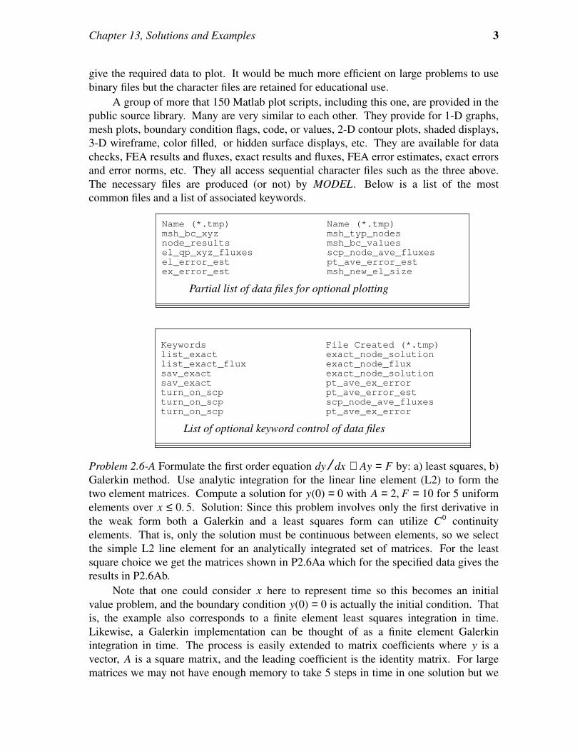
give the required data to plot. It would be much more efficient on large problems to use
binary files but the character files are retained for educational use.
A group of more that 150 Matlab plot scripts, including this one, are provided in the
public source library. Many are very similar to each other. They provide for 1-D graphs,
mesh plots, boundary condition flags, code, or values, 2-D contour plots, shaded displays,
3-D wireframe, color filled, or hidden surface displays, etc. They are available for data
checks, FEA results and fluxes, exact results and fluxes, FEA error estimates, exact errors
and error norms, etc. They all access sequential character files such as the three above.
The necessary files are produced (or not) by MODEL. Below is a list of the most
common files and a list of associated keywords.
Name (*.tmp) Name (*.tmp)msh_bc_xyz msh_typ_nodesnode_results msh_bc_valuesel_qp_xyz_fluxes scp_node_ave_fluxesel_error_est pt_ave_error_estex_error_est msh_new_el_size
Partial list of data files for optional plotting
Keywords File Created (*.tmp)list_exact exact_node_solutionlist_exact_flux exact_node_fluxsav_exact exact_node_solutionsav_exact pt_ave_ex_errorturn_on_scp pt_ave_error_estturn_on_scp scp_node_ave_fluxesturn_on_scp pt_ave_ex_error
List of optional keyword control of data files
Problem 2.6-A Formulate the first order equation dy / dx + Ay = F by: a) least squares, b)
Galerkin method. Use analytic integration for the linear line element (L2) to form the
two element matrices. Compute a solution for y(0) = 0 with A = 2, F = 10 for 5 uniform
elements over x ≤ 0. 5. Solution: Since this problem involves only the first derivative in
the weak form both a Galerkin and a least squares form can utilize C0 continuity
elements. That is, only the solution must be continuous between elements, so we select
the simple L2 line element for an analytically integrated set of matrices. For the least
square choice we get the matrices shown in P2.6Aa which for the specified data gives the
results in P2.6Ab.
Note that one could consider x here to represent time so this becomes an initial
value problem, and the boundary condition y(0) = 0 is actually the initial condition. That
is, the example also corresponds to a finite element least squares integration in time.
Likewise, a Galerkin implementation can be thought of as a finite element Galerkin
integration in time. The process is easily extended to matrix coefficients where y is a
vector, A is a square matrix, and the leading coefficient is the identity matrix. For large
matrices we may not have enough memory to take 5 steps in time in one solution but we

4 Finite Element Analysis with Error Estimators
function true_result_1d_graph (i_p, Exact) ! 1% ------------------------------------------------------ ! 2% Graph FEA & Exact_Case i_p-th component values ! 3% If i_p = 0, show RMS value ! 4% ------------------------------------------------------ ! 5
! 6% nod_per_el = Nodes per element ! 7% np = Number of Points ! 8% nr = Number of results per node ! 9% nt = Number of elements ! 10% t_x = x coordinates of nod_per_el corners ! 11% t_nodes = nodes on an element ! 12% x = all x-coordinates ; ax for analytic ! 13% y = result component i_p ; ar for analytic ! 14
! 15% msh_typ_nodes = connectivity list, nt x nod_per_el ! 16% msh_bc_xyz = nodal coordinates, np x 1 ! 17% node_results = nodal result values, np x nr ! 18
! 19if ( nargin < 2 ) ! 20
error (’No solution given for Exact_Case number’) ! 21end % if no arguments ! 22pre_e = 0 ; % items before connectivity list ! 23pre_p = 1 ; % items before coordinates (BC flag) ! 24
! 25% Read coordinate, connectivity and result files ! 26
load msh_bc_xyz.tmp ; load msh_typ_nodes.tmp ; ! 27load node_results.tmp ; ! 28
! 29% Set control data: ! 30
np = size (msh_bc_xyz,1) ; % number of nodal points ! 31nr = size (node_results, 1) ; % dof per node ! 32nt = size (msh_typ_nodes,1) ; % number of elements ! 33nod_per_el = size (msh_typ_nodes,2) - pre_e -1 ; % nodes ! 34max_p = size (node_results, 2) ; % number of results ! 35
! 36% Optional pre-allocation of arrays, get x coords ! 37
x (np) = 0. ; y (np) = 0. ; t_nodes (nod_per_el) = 0 ; ! 38t_x (nod_per_el) = 0 ; t_y (nod_per_el) = 0 ; ! 39x = msh_bc_xyz (1:np, (pre_p+1)) ; % extract x column ! 40xmax = max (x) ; xmin = min (x) ; % x range to plot ! 41
! 42% add analytic points (12 per element) ! 43
a_inc = (xmax-xmin)/(10*nt) ; ax = [xmin:a_inc:xmax] ; ! 44[ar] = analytic_1_d_result (i_p, ax, Exact) % result ! 45maxa = max (ar) ; mina = min (ar) ; % range ! 46
! 47if ( i_p >= 1 ) % get FEA nodal results ! 48
y = node_results(:, i_p) ; ! 49else % i_p = 0, get root mean square value ! 50
for k = 1:np ! 51y (k) = sqrt ( sum (node_results (k, 1:max_p).ˆ2)) ; ! 52
end % for k ! 53end % if get RMS value ! 54maxy = max (y) ; miny = min (y) ; % range ! 55
! 56
Problem P2.1Ac Gather data for a FEA and analytic graph

Chapter 13, Solutions and Examples 5
% Cite max, min FEA values and locations ! 57[V_X, L_X] = max (y) ; [V_N, L_N] = min (y) ; ! 58fprintf (’Max value is %g at node %g \n’, V_X, L_X) ! 59fprintf (’Min value is %g at node %g \n’, V_N, L_N) ! 60null (1:np) = V_N ; % to locate labels ! 61
! 62% finalize axes ! 63
ymax = max ([maxy, maxa]) ; ymin = min ([miny, mina]) ;! 64clf ; hold on ; % clear graphics, hold ! 65axis ([xmin, xmax, ymin, ymax]) % set axes ! 66xlabel (’X, Node number at 45, Element number at 90 deg’) ! 67
! 68if ( i_p >= 1 ) ! 69
title([’Exact (dash) & FEA Solution Component\_’, ... ! 70int2str(i_p),’: ’, int2str(nt),’ Elements, ’, ... ! 71int2str(np),’ Nodes’]) ! 72
ylabel ([’Component ’, int2str(i_p), ’ (max = ’, ... ! 73num2str(V_X), ’, min = ’, num2str(V_N), ’)’]) ! 74
! 75else % i_p = 0, get root mean sq ! 76
title([’Exact (dash) & FEA RMS\_value: ’, ... ! 77int2str(nt),’ Elements, ’, int2str(np),’ Nodes’]) ! 78
ylabel ([’Solution RMS Value (max = ’, ... ! 79num2str(V_X), ’, min = ’, num2str(V_N), ’)’]) ! 80
end % if get RMS value ! 81! 82
plot (ax, ar, ’r--’) % add analytic plot first ! 83! 84
for it = 1:nt ; % Loop over all elements ! 85! 86
% Extract element connectivity & coordinates ! 87t_nodes = msh_typ_nodes(it,(pre_e+2):(nod_per_el+pre_e+1));! 88t_x = x (t_nodes) ; t_y = y (t_nodes) ; % coordinates ! 89
! 90% Plot the element number, graph element result ! 91
x_bar = sum (t_x’ )/nod_per_el ; % centroid ! 92t_text = sprintf (’ (%g)’, it); % offset # from pt ! 93text (x_bar, V_N, t_text, ’Rotation’, 90) % incline ! 94plot (x_bar, V_N, ’k+’) % element number ! 95plot (t_x, t_y) % element lines ! 96end % for over all elements ! 97
! 98for i = 1:np % plot node points on axis ! 99
t_text = sprintf (’ %g’, i); % offset # from pt !100text (x(i), null(i), t_text, ’Rotation’, 45) % incline !101
end % for all node numbers, Add * at nodes !102plot (x, null, ’k*’) ; grid ; hold off !103
% end of true_result_1d_graph !104
Problem P2.1Ad Plotting a FEA and analytic graph

6 Finite Element Analysis with Error Estimators
! ............................................................ ! 1! *** ELEM_SQ_MATRIX PROBLEM DEPENDENT STATEMENTS FOLLOW *** ! 2! ............................................................ ! 3! APPLICATION: LEAST SQUARES SOLUTION OF Y’ + A * Y = F ! 4! Exact solution: y(x) = (1 - e (-Ax)) * F / A, with y(0) = 0 ! 5! N_SPACE = 1, NOD_PER_EL = 2, N_G_DOF = 1 ! 6REAL(DP), SAVE :: A, F, DL ! GLOBAL DATA, ELEMENT LENGTH ! 7
! 8! RECOVER GLOBAL PROBLEM COEFFICIENTS, A AND F (ON FIRST CALL) ! 9
IF ( THIS_EL == 1 ) THEN ! Get coefficients !10A = GET_REAL_MISC (1) ; F = GET_REAL_MISC (2) !12
END IF ! First call !13DL = COORD (2, 1) - COORD (1, 1) ! ELEMENT LENGTH !14
!15! EXACT INTEGRATION SQUARE MATRIX AND SOURCE VECTOR !16
S (1, 1) = (3.d0 - 3.d0 * A * DL + A * A * DL * DL) / 3 / DL !17S (2, 2) = (3.d0 + 3.d0 * A * DL + A * A * DL * DL) / 3 / DL !18S (1, 2) = (A * A * DL * DL - 6.d0) / 6.d0 / DL !19S (2, 1) = S (1, 2) !20C (1) = 0.5d0 * F * (A * DL - 2.d0) !21C (2) = 0.5d0 * F * (A * DL + 2.d0) !22
! *** END ELEM_SQ_MATRIX PROBLEM DEPENDENT STATEMENTS *** !23
Problem P2.6Aa Element matrices from exact integration
TITLE "LEAST SQUARES SOLUTION OF Y’+2Y=10, Y(0) = 0" ! 1THE NEXT 3 LINES ARE USER SUPPLIED ! 21 LEAST SQUARES SOLUTION OF Y’+2Y=10, Y(0) = 0 ! 32 Exact solution = 5(1 - eˆ(-2x)) ! 43 This is example 103 in the source library ! 5
*** NODAL POINT DATA *** ! 6NODE, BC_FLAG, X-Coord, ! 7
1 1 0.0000 ! 82 0 0.1000 ! 93 0 0.2000 !104 0 0.3000 !115 0 0.4000 !126 0 0.5000 !13
*** ELEMENT CONNECTIVITY DATA *** !14ELEMENT, 2 NODAL INCIDENCES. !15
1 1 2 !162 2 3 !173 3 4 !184 4 5 !195 5 6 !20
*** CONSTRAINT EQUATION DATA *** !21EQ. NO. NODE_1 PAR_1 A_1 !22
1 1 1 0.00000E+00 !23*** MISCELLANEOUS SYSTEM PROPERTIES *** !24PROPERTY REAL_VALUE !25
1 2.00000E+00 !262 1.00000E+01 !27
*** OUTPUT OF RESULTS IN NODAL ORDER *** !28NODE, X-Coord, DOF_1, EXACT1, !29
1 0.0000E+00 0.0000E+00 0.0000E+00 !302 1.0000E-01 9.0749E-01 9.0635E-01 !313 2.0000E-01 1.6502E+00 1.6484E+00 !324 3.0000E-01 2.2580E+00 2.2559E+00 !335 4.0000E-01 2.7554E+00 2.7534E+00 !346 5.0000E-01 3.1624E+00 3.1606E+00 !35
Problem P2.6Ab Results for 5 L2 elements

Chapter 13, Solutions and Examples 7
0 0.1 0.2 0.3 0.4 0.5 0.6 0.7 0.8 0.9 10
0.01
0.02
0.03
0.04
0.05
0.06
0.07
X, Node at 45 deg (2 per element), Element at 90 deg
Exact (dash) & Linear FEA Component_1: 3 Elements, 4 Nodes (2 per Element)
Com
pone
nt 1
(m
ax =
0.0
6751
4, m
in =
0)
(1
)
(2
)
(3
)
1
2
3
4
−−−min
−−−max
U’’ + U + x = 0U(0) = 0U(1) = 0
Problem P2.13a Three linear element Galerkin solution results
0 0.1 0.2 0.3 0.4 0.5 0.6 0.7 0.8 0.9 1−0.35
−0.3
−0.25
−0.2
−0.15
−0.1
−0.05
0
0.05
0.1
0.15
X, Node number at 45 deg, Element number at 90 deg
Exact (dash), Linear FEA (solid) Flux Component_1: 3 Elements, 4 Nodes
Flu
x C
ompo
nent
1
(1
)
(2
)
(3
)
1
2
3
4
U’’ + U + x = 0U(0) = 0U(1) = 0
Problem P2.13b Three linear element gradient results

8 Finite Element Analysis with Error Estimators
could solve one step in time repeatedly and use the answer for the first step (here y(0. 1))
as the initial condition for the next step. Taking more than one step in time in a single
solution, when feasible, can reduce the error in the time integration.
Problem 2.13 Use three equal length elements to solve the problem in Fig. 2.10.6
(Le = 1/3). Obtain the nodal values, reactions, and post-process for the element
gradients. Compare the nodal values to the exact solution. Solution: As expected, the
results fall between those seen in Figs. 2.10.6 and 7, and are summarized here in Figs.
P2.13 a and 13b. The nodal values are moving closer to the correct values. The solution
is most accurate at the nodes, but the slopes (gradients) are discontinuous there. The
slopes are most accurate near the center of each element.
Problem 2.15 Solve Eq 2.43 for a non-zero Neumann condition of
du/dx(1) = Cotan(1) − 1 and u(0) = 0, and compare the results to the same exact
solution. Solution: Changing the Dirichlet boundary condition at the right end to a
Neumann natural condition (qL = 0) not only changes the analytic solution but also
shows an approximation behavior that is quite different from a boundary value problem.
That is because the slope boundary condition at the right is satisfied only in the weak
sense. In other words, neither the solution value or slope is exact at the right end. In
particular, there is a noticeable difference in P2.15a and P2.15b between the slope of the
last element and the specified rightmost slope. This is generally true and the user can
partially compensate for that by making the element lengths smaller as they approach
(normal to) a Neumann boundary condition. Of course, going to higher order elements
also reduces the slope differences at such a boundary. If you used the same number of
degrees of freedom in a single cubic Lagrangian element both the solution and slope
would be much more accurate. A cubic Hermite element would convert the Neumann
condition to a Dirichlet condition on its nodal slope value and thus give an exact slope on
the boundary. Howev er, that might over constrain the interior solution if the given data
were not smooth over space.
Problem 2.16 The exact solution of d2u / dx2 + Q(x) = 0 with u(0) = 0 = u(1) with
Q = 1 for x ≤ 1/2 and 0 for x > 1/2 is u(x) = x(3 − 4x)/8 for x ≤ 1/2 othewise
U(x) = (1 − x)/8. The assembled source vector for length ratios of 1:1:2 is
CTQ = [1 2 1 0]/8 while for three equal length elements it is CT
Q = [4 7 1 0]/24.
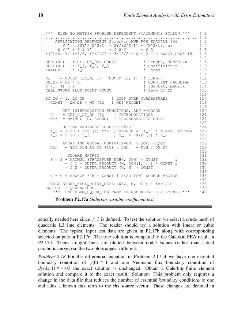
Problem 2.17 Obtain a Galerkin solution of y′′ − 2y′ x / g + 2y / g = g, for g = (x2 + 1),
on 0 ≤ x ≤ 1 with the boundary conditions y(0) = 2, y(1) = 5 / 3. Solution: This requires
only a C0 approximation since the weak form involves only the first derivative of y when
the first term is integrated by parts. Since the variable coefficients are rational
polynomials it would be complicated to try to evaluate the matrices by exact integration
so we use numerical integration. For the same reason, Gaussian quadratures will not be
exact so we select a moderate number of quadrature points as a balance between accuracy
and computational cost. This implementation supports all one-dimension elements in the
library and is displayed in P2.17a.
Note, in lines 25-26, that the variable coefficients have been hard coded rather than
using an include file or user function. The variable SOURCE is a global item that can
sometimes be assigned constant values through keyword data controls. It was not

Chapter 13, Solutions and Examples 9
0 0.1 0.2 0.3 0.4 0.5 0.6 0.7 0.8 0.9 10
0.1
0.2
0.3
0.4
0.5
X, Node at 45 deg (2 per element), Element at 90 deg
Exact (dash) & Linear FEA Component_1: 3 Elements, 4 Nodes (2 per Element)
Com
pone
nt 1
(m
ax =
0.5
4904
, min
= 0
)
(1
)
(2
)
(3
)
1
2
3
4
−−−min
−−−max
U’’ + U + x = 0U(0) = 0dU/dx (1) = 0
Problem P2.15a Three element solution for a natural BC
0 0.1 0.2 0.3 0.4 0.5 0.6 0.7 0.8 0.9 10
0.1
0.2
0.3
0.4
0.5
0.6
0.7
0.8
X, Node number at 45 deg, Element number at 90 deg
Exact (dash), Linear FEA (solid) Flux Component_1: 3 Elements, 4 Nodes
Flu
x C
ompo
nent
1
(1
)
(2
)
(3
)
1
2
3
4
U’’ + U + x = 0U(0) = 0dU/dx (1) = 0
Problem P2.15b Three element gradients for a natural BC
10 Finite Element Analysis with Error Estimators
! *** ELEM_SQ_MATRIX PROBLEM DEPENDENT STATEMENTS FOLLOW *** ! 1! .............................................................. ! 2! APPLICATION DEPENDENT Galerkin MWR FOR EXAMPLE 106 ! 3! Y’’ - 2XY’/(Xˆ2+1) + 2Y/(Xˆ2+1) = (Xˆ2+1), or ! 4! E Y’’ + f_1 Y’ + f_2 Y = f_3 ! 5! Y(0)=2, Y(1)=5/3, Y=Xˆ4/6 - 3Xˆ2/2 + X + 2 (is EXACT_CASE 15) ! 6
! 7REAL(DP) :: DL, DX_DR, CONST ! Length, Jacobian ! 8REAL(DP) :: f_1, f_2, f_3 ! Coefficients ! 9INTEGER :: IQ ! Loops !10
!11DL = COORD (LT_N, 1) - COORD (1, 1) ! LENGTH !12DX_DR = DL / 2. ! CONSTANT JACOBIAN !13E (1, 1) = 1 ! identity matrix !14CALL STORE_FLUX_POINT_COUNT ! Save LT_QP !15
!16DO IQ = 1, LT_QP ! LOOP OVER QUADRATURES !17
CONST = DX_DR * WT (IQ) ! NET WEIGHT !18!19
! GET INTERPOLATION FUNCTIONS, AND X-COORD !20H = GET_H_AT_QP (IQ) ! INTERPOLATIONS !21XYZ = MATMUL (H, COORD) ! ISOPARAMETRIC POINT !22
!23! DEFINE VARIABLE COEFFICIENTS !24
f_3 = 1.d0 + XYZ (1) **2 ; SOURCE = -f_3 ! global source !25f_2 = 2.d0 / f_3 ; f_1 = -XYZ (1) * f_2 !26
!27! LOCAL AND GLOBAL DERIVATIVES, dH/dr, dH/dx !28
DLH = GET_DLH_AT_QP (IQ) ; DGH = DLH / DX_DR !29!30
! SQUARE MATRIX !31S = S + MATMUL (TRANSPOSE(DGH), DGH) * CONST & !32
- f_1 * OUTER_PRODUCT (H, DGH(1, :)) * CONST & !33- f_2 * OUTER_PRODUCT (H, H) * CONST !34
!35C = C + SOURCE * H * CONST ! RESULTANT SOURCE VECTOR !36
!37CALL STORE_FLUX_POINT_DATA (XYZ, E, DGH) ! for SCP !38
END DO ! QUADRATURE !39! *** END ELEM_SQ_EX_106 PROBLEM DEPENDENT STATEMENTS *** !40
Problem P2.17a Galerkin variable coefficient test
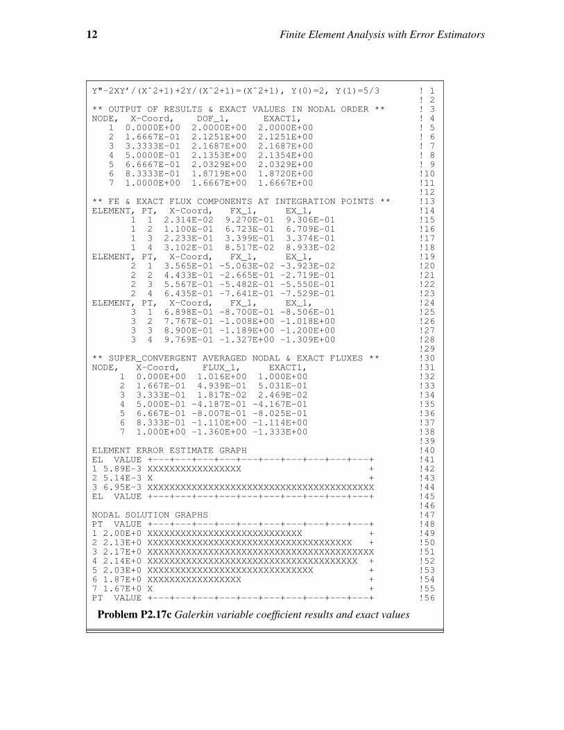
actually needed here since f _3 is defined. To test the solution we select a crude mesh of
quadratic L3 line elements. The reader should try a solution with linear or cubic
elements. The typical input test data are given in P2.17b along with corresponding
selected outputs in P2.17c. The true solution is compared to the Galerkin FEA result in
P2.17d. There straight lines are plotted between nodal values (rather than actual
parabolic curves) so the two plots appear different.
Problem 2.18 For the differential equation in Problem 2.17 if we have one essential
boundary condition of y(0) = 1 and one Neumann flux boundary condition of
dy/dx(1) = − 4/3 the exact solution is unchanged. Obtain a Galerkin finite element
solution and compare it to the exact result. Solution: This problem only requires a
change in the data file that reduces the number of essential boundary conditions to one
and adds a known flux term to the rhs source vector. These changes are denoted in

Chapter 13, Solutions and Examples 11
title "Y’’ - 2XY’/(Xˆ2+1) + 2Y/(Xˆ2+1) = (Xˆ2+1)" ! 1nodes 7 ! Number of nodes in the mesh ! 2elems 3 ! Number of elements in the system ! 3dof 1 ! Number of unknowns per node ! 4el_nodes 3 ! Maximum number of nodes per element ! 5space 1 ! Solution space dimension ! 6b_rows 1 ! Number of rows in B (operator) matrix ! 7el_react ! Compute & list element reactions ! 8gauss 4 ! Maximum number of quadrature points ! 9exact_case 15 ! Exact analytic solution !10scp_neigh_el ! Default SCP patch group type !11unsymmetric ! Unsymmetric skyline storage is used !12list_exact ! List exact answers at nodes !13list_exact_flux ! List exact fluxes at nodes !14bar_chart ! print-plot result !15remarks 4 ! Number of user remarks !16quit ! keyword input, remarks follow !17Galerkin: Y’’ - 2XY’/(Xˆ2+1) + 2Y/(Xˆ2+1) = (Xˆ2+1) !18with Y(0)=2, Y(1)=5/3, Y(X) = Xˆ4/6 - 3Xˆ2/2 + X + 2 !19Fausett p. 482, EXACT_CASE = 15 !20Here we use three quadratic (L3) line elements. !211 1 0. ! node bc_flag x !222 0 0.166666667 ! node bc_flag x !233 0 0.333333333 ! node bc_flag x !244 0 0.5 ! node bc_flag x !255 0 0.666666667 ! node bc_flag x !266 0 0.833333334 ! node bc_flag x !277 1 1.00 ! node bc_flag x !281 1 2 3 ! elem j, k, l !292 3 4 5 ! elem j, k, l !303 5 6 7 ! elem j, k, l !311 1 2. ! Essential BC: node dof_value !327 1 1.66666667 ! Essential BC: node dof_value !33
Problem P2.17b Galerkin L2 model test data
P2.18a. External source vector components are initialized to zero. The keyword loads
requires the non-zero entries to be input (after the EBC and MPC) by giving the node
number, degree of freedom number, and corresponding known flux. The data ends with
the last dof flux value (which is usually zero). The output is unchanged except for
echoing the above lines and listing the initial external source vector terms, in P2.18b.
1.3 Problems from chapter 3
Problem 3.1 For a one-dimensional quadratic element use the unit coordinate
interpolation functions in Fig. 3.4.1 to evaluate the matrices:
a) Ce = ∫LeHT dx, b) Me = ∫Le
HT H dx ,
c) Se = ∫Le
dHT
dx
dH
dxdx , d) Ue = ∫Le
HT dH
dxdx , and
Problem 3.2 Solve the above problem by using the natural coordinate version,
−1 ≤ n ≤ 1, from Fig, 3.4.1. Solution: Either local coordinate system must lead to the
12 Finite Element Analysis with Error Estimators
Y"-2XY’/(Xˆ2+1)+2Y/(Xˆ2+1)=(Xˆ2+1), Y(0)=2, Y(1)=5/3 ! 1! 2
** OUTPUT OF RESULTS & EXACT VALUES IN NODAL ORDER ** ! 3NODE, X-Coord, DOF_1, EXACT1, ! 4
1 0.0000E+00 2.0000E+00 2.0000E+00 ! 52 1.6667E-01 2.1251E+00 2.1251E+00 ! 63 3.3333E-01 2.1687E+00 2.1687E+00 ! 74 5.0000E-01 2.1353E+00 2.1354E+00 ! 85 6.6667E-01 2.0329E+00 2.0329E+00 ! 96 8.3333E-01 1.8719E+00 1.8720E+00 !107 1.0000E+00 1.6667E+00 1.6667E+00 !11
!12** FE & EXACT FLUX COMPONENTS AT INTEGRATION POINTS ** !13ELEMENT, PT, X-Coord, FX_1, EX_1, !14
1 1 2.314E-02 9.270E-01 9.306E-01 !151 2 1.100E-01 6.723E-01 6.709E-01 !161 3 2.233E-01 3.399E-01 3.374E-01 !171 4 3.102E-01 8.517E-02 8.933E-02 !18
ELEMENT, PT, X-Coord, FX_1, EX_1, !192 1 3.565E-01 -5.063E-02 -3.923E-02 !202 2 4.433E-01 -2.665E-01 -2.719E-01 !212 3 5.567E-01 -5.482E-01 -5.550E-01 !222 4 6.435E-01 -7.641E-01 -7.529E-01 !23
ELEMENT, PT, X-Coord, FX_1, EX_1, !243 1 6.898E-01 -8.700E-01 -8.506E-01 !253 2 7.767E-01 -1.008E+00 -1.018E+00 !263 3 8.900E-01 -1.189E+00 -1.200E+00 !273 4 9.769E-01 -1.327E+00 -1.309E+00 !28
!29** SUPER_CONVERGENT AVERAGED NODAL & EXACT FLUXES ** !30NODE, X-Coord, FLUX_1, EXACT1, !31
1 0.000E+00 1.016E+00 1.000E+00 !322 1.667E-01 4.939E-01 5.031E-01 !333 3.333E-01 1.817E-02 2.469E-02 !344 5.000E-01 -4.187E-01 -4.167E-01 !355 6.667E-01 -8.007E-01 -8.025E-01 !366 8.333E-01 -1.110E+00 -1.114E+00 !377 1.000E+00 -1.360E+00 -1.333E+00 !38
!39ELEMENT ERROR ESTIMATE GRAPH !40EL VALUE +---+---+---+---+---+---+---+---+---+---+ !411 5.89E-3 XXXXXXXXXXXXXXXXX + !422 5.14E-3 X + !433 6.95E-3 XXXXXXXXXXXXXXXXXXXXXXXXXXXXXXXXXXXXXXXXX !44EL VALUE +---+---+---+---+---+---+---+---+---+---+ !45
!46NODAL SOLUTION GRAPHS !47PT VALUE +---+---+---+---+---+---+---+---+---+---+ !481 2.00E+0 XXXXXXXXXXXXXXXXXXXXXXXXXXXX + !492 2.13E+0 XXXXXXXXXXXXXXXXXXXXXXXXXXXXXXXXXXXXX + !503 2.17E+0 XXXXXXXXXXXXXXXXXXXXXXXXXXXXXXXXXXXXXXXXX !514 2.14E+0 XXXXXXXXXXXXXXXXXXXXXXXXXXXXXXXXXXXXXX + !525 2.03E+0 XXXXXXXXXXXXXXXXXXXXXXXXXXXXXX + !536 1.87E+0 XXXXXXXXXXXXXXXXX + !547 1.67E+0 X + !55PT VALUE +---+---+---+---+---+---+---+---+---+---+ !56
Problem P2.17c Galerkin variable coefficient results and exact values

Chapter 13, Solutions and Examples 13
0 0.1 0.2 0.3 0.4 0.5 0.6 0.7 0.8 0.9 1
1.7
1.75
1.8
1.85
1.9
1.95
2
2.05
2.1
2.15
X, Node at 45 deg (3 per element), Element at 90 deg
Exact (dash) & Quadratic FEA Component_1: 3 Elements, 7 Nodes (3 per Element)C
ompo
nent
1 (
max
= 2
.168
7, m
in =
1.6
667)
(1
)
(2
)
(3
)
1
2
3
4
5
6
7
−−−min
−−−max
Y’’ − 2XY’ / (X2+1) + 2Y / (X2+1) = (X2+1)
Y(0) = 2, Y(1) = 5/3
Y(X) = X4 / 6 − 3X2 / 2 + X + 2
Problem P2.17d True solution and Galerkin nodal values
loads ! An initial source vector is input !11Galerkin: Y’’ - 2XY’/(Xˆ2+1) + 2Y/(Xˆ2+1) = (Xˆ2+1) !18with Y(0)=2, Y’(1)=-4/3, Y(X) = Xˆ4/6 - 3Xˆ2/2 + X + 2 !197 0 1.00 ! removed EBC flag !287 1 -1.33333 ! Enter only (last) non-zero source term !33
Problem P2.18a Galerkin L2 data changes for Neumann condition
. . . !1*** INITIAL FORCING VECTOR DATA *** !2
NODE PARAMETER VALUE EQUATION !37 1 -1.33333E+00 7 !4
*** RESULTANTS *** !5COMPONENT SUM POSITIVE NEGATIVE !6IN_1, -1.3333E+00 0.0000E+00 -1.3333E+00 !7
Problem P2.18b Galerkin L2 output changes for Neumann condition
14 Finite Element Analysis with Error Estimators
same final result, if one treats the Jacobian correctly. The exact integrals are listed in
subroutine form in Problem P3.1. Note that the last square matrix is unsymmetrical. In
our usual notation these give:
Ce =Le
6
1
4
1
, Me =Le
30
4
2
−1
2
16
2
−1
2
4
,
Se =1
3 Le
7
−8
1
−8
16
−8
1
−8
7
, Ue =1
6
−3
−4
1
4
0
−4
−1
4
3
.
Can you explain why Le is in the numerator, denominator, or missing in each matrix?
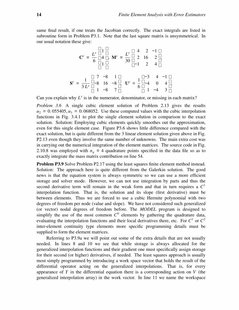
Problem 3.6 A single cubic element solution of Problem 2.13 gives the results
u2 = 0. 055405, u3 = 0. 068052. Use these computed values with the cubic interpolation
functions in Fig. 3.4.1 to plot the single element solution in comparison to the exact
solution. Solution: Employing cubic elements quickly smoothes out the approximation,
ev en for this single element case. Figure P3.6 shows little difference compared with the
exact solution, but is quite different from the 3 linear element solution given above in Fig.
P2.13 even though they inv olve the same number of unknowns. The main extra cost was
in carrying out the numerical integration of the element matrices. The source code in Fig.
2.10.8 was employed with nq = 4 quadrature points specified in the data file so as to
exactly integrate the mass matrix contribution on line 54.
Problem P3.9 Solve Problem P2.17 using the least squares finite element method instead.
Solution: The approach here is quite different from the Galerkin solution. The good
news is that the equation system is always symmetric so we can use a more efficient
storage and solver mode. However, we can not use integration by parts and thus the
second derivative term will remain in the weak form and that in turn requires a C1
interpolation function. That is, the solution and its slope (first derivative) must be
between elements. Thus we are forced to use a cubic Hermite polynomial with two
degrees of freedom per node (value and slope). We hav e not considered such generalized
(or vector) nodal degrees of freedom before. The MODEL program is designed to
simplify the use of the most common C0 elements by gathering the quadrature data,
evaluating the interpolation functions and their local derivatives there, etc. For C1 or C2
inter-element continuity type elements more specific programming details must be
supplied to form the element matrices.
Referring to P3.9a we will point out some of the extra details that are not usually
needed. In lines 8 and 10 we see that while storage is always allocated for the
generalized interpolation functions and their gradient one must specifically assign storage
for their second (or higher) derivatives, if needed. The least squares approach is usually
most simply programmed by introducing a work space vector that holds the result of the
differential operator acting on the generalized interpolations. That is, for every
appearance of Y in the differential equation there is a corresponding action on V (the
generalized interpolation array) in the work vector. In line 11 we name the workspace

Chapter 13, Solutions and Examples 15
SUBROUTINE INTEGRAL_H_ON_L3 (LENGTH, C_E) ! 1! *-* *-* *-* *-* *-* *-* *-* *-* *-* *-* *-* *-* *-* ! 2! INTEGRATE SHAPE FUNCTIONS OF A 3 NODE LINE ELEMENT ! 3! *-* *-* *-* *-* *-* *-* *-* *-* *-* *-* *-* *-* *-* ! 4Use Precision_Module ! for DP ! 5IMPLICIT NONE ! 6REAL(DP), INTENT(IN) :: LENGTH ! PHYSICAL LENGTH ! 7REAL(DP), INTENT(OUT) :: C_E (3) ! INTEGRAL OF H ! 8
! LOCAL NODE COORD. ARE -1,0,+1 1-----2-----3 ! 9!10
C_E = LENGTH * (/ 1.d0, 4.d0, 1.d0 /) / 6.d0 !11END SUBROUTINE INTEGRAL_H_ON_L3 !12
!13SUBROUTINE INTEGRAL_HT_H_ON_L3 (LENGTH, MASS_E) !14! *-* *-* *-* *-* *-* *-* *-* *-* *-* *-* *-* *-* *-* !15! INTEGRATE H-TRANSPOSE H ON A 3 NODE LINE ELEMENT !16! *-* *-* *-* *-* *-* *-* *-* *-* *-* *-* *-* *-* *-* !17Use Precision_Module ! for DP !18IMPLICIT NONE !19REAL(DP), INTENT(IN) :: LENGTH ! PHYSICAL LENGTH !20REAL(DP), INTENT(OUT) :: MASS_E (3, 3) ! INTEGRAL OF H’ H !21REAL(DP), PARAMETER :: MASS (3, 3) = RESHAPE ( & !22
(/ 4, 2, -1, 2, 16, 2, -1, 2, 4 /), (/3, 3/) ) / 30.d0 !23! LOCAL NODE COORD. ARE -1,0,+1 1-----2-----3 !24
!25MASS_E = LENGTH * MASS !26
END SUBROUTINE INTEGRAL_HT_H_ON_L3 !27!28
SUBROUTINE INTEGRAL_DHDXT_DHDX_ON_L3 (LENGTH, STIFF_E) !29! *-* *-* *-* *-* *-* *-* *-* *-* *-* *-* *-* *-* *-* !30! INTEGRATE DHDX-TRANSPOSE DHDX ON A 3 NODE LINE ELEMENT !31! *-* *-* *-* *-* *-* *-* *-* *-* *-* *-* *-* *-* *-* !32Use Precision_Module ! for DP !33IMPLICIT NONE !34REAL(DP), INTENT(IN) :: LENGTH !PHYSICAL LENGTH !35REAL(DP), INTENT(OUT):: STIFF_E (3, 3) !INTEGRAL DHDX’ DHDX !36REAL(DP), PARAMETER :: STIFF (3, 3) = RESHAPE ( & !37
(/ 7, -8, 1, -8, 16, -8, 1, -8, 7/), (/3, 3/) ) / 3.d0 !38! LOCAL NODE COORD. ARE -1,0,+1 1-----2-----3 !39
!40STIFF_E = STIFF / LENGTH !41
END SUBROUTINE INTEGRAL_DHDXT_DHDX_ON_L3 !42!43
SUBROUTINE INTEGRAL_HT_DHDX_ON_L3 (U_E) !44! *-* *-* *-* *-* *-* *-* *-* *-* *-* *-* *-* *-* *-* !45! INTEGRATE H-TRANSPOSE DHDX ON A 3 NODE LINE ELEMENT !46! *-* *-* *-* *-* *-* *-* *-* *-* *-* *-* *-* *-* *-* !47Use Precision_Module ! for DP !48IMPLICIT NONE !49REAL(DP), INTENT(OUT) :: U_E (3, 3) ! INTEGRAL H’ DHDX !50REAL(DP), PARAMETER :: U (3, 3) = RESHAPE ( & !51
(/ -3, -4, 1, 4, 0, -4, -1, 4, 3/), (/3, 3/) ) / 6.d0 !52! LOCAL NODE COORD. ARE -1,0,+1 1-----2-----3 !53
!54U_E = U !55
END SUBROUTINE INTEGRAL_HT_DHDX_ON_L3 !56
Problem P3.1 Typical quadratic C0 element integrals

16 Finite Element Analysis with Error Estimators
0 0.1 0.2 0.3 0.4 0.5 0.6 0.7 0.8 0.9 10
0.01
0.02
0.03
0.04
0.05
0.06
0.07
X, Node at 45 deg (4 per element), Element at 90 deg
Exact (dash) & FEA Component_1: 1 Elements, 4 Nodes (4 per Element)
Com
pone
nt 1
(m
ax =
0.0
6805
2, m
in =
0)
(1
)
1
2
3
4
−−−min
−−−max
Problem P3.6 A single cubic element model and exact problem solution

Chapter 13, Solutions and Examples 17
! *** ELEM_SQ_MATRIX PROBLEM DEPENDENT STATEMENTS FOLLOW *** ! 1! ............................................................ ! 2! LEAST SQ. SOL. OF: Y’’ - 2XY’/(Xˆ2+1) + 2Y/(Xˆ2+1) = (Xˆ2+1) ! 3! USING 3-RD ORDER HERMITE IN UNIT COORDINATES ! 4! CONVERTED FROM NATURAL COORDINATES ! 5! >>> NOTE NOT SCALAR INTERPOLATION, C_1 ELEMENTS <<< ! 6! ------------------------------------------- ! 7! Allocated V (LT_FREE) and DGV (N_SPACE, LT_FREE) by MODEL ! 8
! 9REAL(DP) :: D2GV (LT_FREE) ! v’’, 2nd derivative !10REAL(DP) :: OP_V (LT_FREE) ! ODE on H array !11REAL(DP) :: PT_UNIT, WT_UNIT ! unit coord pt, weight !12REAL(DP) :: DL, X_SQ, X_G ! physical length, pt !13INTEGER :: IP ! loops !14
!15! V = GENERALIZED (VECTOR) INTERPOLATION FUNCTIONS !16! DGV = DERIVATIVE OF GENERALIZED (VECTOR) INTERPOLATION !17! D2GV = 2nd DERIVATIVE OF GENERALIZED (VECTOR) INTERPOLATION !18
!19IF ( DEBUG_EL_SQ ) WRITE (N_BUG, *) ’Enter my_sq_matrix_inc’ !20
!21E = GET_REAL_IDENTITY (N_R_B) ! DUMMY CONSTITUTIVE !22DL = COORD (2, 1) - COORD (1, 1) ! GET THE LENGTH !23CALL STORE_FLUX_POINT_COUNT ! Save LT_QP !24
!25! NUMERICAL INTEGRATION LOOP !26
DO IP = 1, LT_QP !27!28
!--> FIND UNIT COORDINATES AND WEIGHT FOR INTEGRATION !29PT_UNIT = (1.d0 + PT(1,IP)) / 2.d0 ! Convert pt !30WT_UNIT = WT (IP) / 2.0d0 ! Convert wt !31XYZ (1) = COORD (1, 1) + PT_UNIT * DL ! Physical pt !32X_SQ = XYZ (1) * XYZ (1) ! x ˆ 2 !33X_G = X_SQ + 1.d0 ! scalar g(x) !34
!35!--> EVALUATE HERMITE SHAPE FUNCTIONS AND DERIVATIVES !36
CALL SHAPE_C1_L (PT_UNIT, DL, V) ! V (NOT H) !37CALL DERIV_C1_L (PT_UNIT, DL, DGV) ! DV / DX !38CALL DERIV2_C1_L (PT_UNIT, DL, D2GV) ! Dˆ2 V / DXˆ2 !39
!40! WORK VECTOR, OP_V = V’’ - 2X V’/(Xˆ2+1) + 2 V/(Xˆ2+1) !41
OP_V = D2GV - 2.d0 * XYZ (1) * DGV(1,:) / X_G & !42+ 2.d0 * V / X_G !43
!44! COMPLETE THE SQUARE MATRIX AND SOURCE VECTOR !45! S_IJ = S_IJ + WT_UNIT * OP_V_I * OP_V_J * DL !46
S = S + WT_UNIT * OUTER_PRODUCT (OP_V, OP_V) * DL !47C = C + WT_UNIT * X_G * OP_V * DL !48
!49! STORE DATA FOR SCP OR POST PROCESSING !50
B (1, :) = DGV (1, :) ; B (2, :) = D2GV (:) !51CALL STORE_FLUX_POINT_DATA (XYZ, E, B) ! for SCP !52
END DO !53! *** END ELEM_SQ_EX_107 PROBLEM DEPENDENT STATEMENTS *** !54
Problem P3.9a A C1 unit coordinate least squares version

18 Finite Element Analysis with Error Estimators
title "Y’’ - 2XY’/(Xˆ2+1) + 2Y/(Xˆ2+1) = (Xˆ2+1)" ! 1nodes 4 ! Number of nodes in the mesh ! 2elems 3 ! Number of elements in the system ! 3dof 2 ! Number of unknowns per node ! 4el_nodes 2 ! Maximum number of nodes per element ! 5space 1 ! Solution space dimension ! 6b_rows 2 ! Number of rows in B (operator) matrix ! 7shape 1 ! Shape, 1=line, 2=tri, 3=quad, 4=hex ! 8gauss 5 ! Maximum number of quadrature points ! 9example 107 ! Source library example number !10data_set 1 ! Data set for example (this file) !11exact_case 15 ! Exact analytic solution !12scp_neigh_el ! Default SCP patch group type !13list_exact ! List exact answers at nodes !14list_exact_flux ! List exact fluxes at nodes !15remarks 4 ! Number of user remarks !16quit ! keyword input !17Least Sq: Y’’ - 2XY’/(Xˆ2+1) + 2Y/(Xˆ2+1) = (Xˆ2+1) !18with Y(0)=2, Y(1)=5/3, Y(X) = Xˆ4/6 - 3Xˆ2/2 + X + 2 !19Fausett p. 482, EXACT_CASE = 15 !20Here we use 3 cubic Hermite (C1_L) line elements. !211 10 0. ! node, 2_binary_ bc_flags, x !222 00 0.333333333 ! node, 2_binary_ bc_flags, x !233 00 0.666666667 ! node, 2_binary_ bc_flags, x !244 10 1.00 ! node, 2_binary_ bc_flags, x !251 1 2 ! elem, j, k !262 2 3 ! elem, j, k !273 3 4 ! elem, j, k !281 1 2. ! Essential BC: node, dof_value !294 1 1.66666667 ! Essential BC: node, dof_value !30
Problem P3.9b Three element least square C1 data set
OP_V (for OPerator acting on V) and assign it the same storage allotment as V . Note
that at any point, the work vector times the element degrees of freedom plus any source
term is the residual error in the differential equation at that point. In other words
OP_V = ∂R / ∂ΦΦ which was defined in Eq. 2.25 as the weighting term in a least squares
formulation. Using this work vector the element square matrix and source vector are
always defined as:
Se = ∫ΩeOP_V T OP_V dΩ, Ce
Q = ∫ΩeOP_V T Q dΩ .
For this specific application the terms required in the work vector are seen by comparing
the comments in lines 3 and 41.
From Fig. 3.5.1 we see that the Hermite family of elements are provided here in unit
coordinates, not in the natural coordinates used to store the Gaussian quadrature data (for
lines). Therefore it is necessary to either convert the quadrature data or re-program all the
Hermite interpolations and derivatives. Lines 12 and 30-31 declare and carry out the
quadrature conversion. Line 13 does the linear unit coordinate interpolation for the
physical X position needed to evaluate the variable coefficients and source term. Lines
37-39 evaluate the Hermite polynomials and the first and second physical derivatives (by
using the element length, DL). One only needs lines 22, 24, 50-52 if SCP or other post-
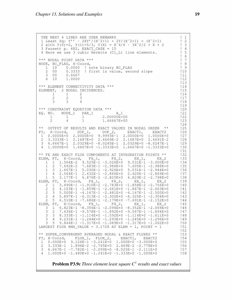
Chapter 13, Solutions and Examples 19
THE NEXT 4 LINES ARE USER REMARKS ! 11 Least Sq: Y’’ - 2XY’/(Xˆ2+1) + 2Y/(Xˆ2+1) = (Xˆ2+1) ! 22 with Y(0)=2, Y(1)=5/3, Y(X) = Xˆ4/6 - 3Xˆ2/2 + X + 2 ! 33 Fausett p. 482, EXACT_CASE = 15 ! 44 Here we use 3 cubic Hermite (C1_L) line elements. ! 5
! 6*** NODAL POINT DATA *** ! 7NODE, BC_FLAG, X-Coord, ! 8
1 10 0.0000 ! note binary BC_FLAG ! 92 00 0.3333 ! first is value, second slope !103 00 0.6667 !114 10 1.0000 !12
!13*** ELEMENT CONNECTIVITY DATA *** !14ELEMENT, 2 NODAL INCIDENCES. !15
1 1 2 !162 2 3 !173 3 4 !18
!19*** CONSTRAINT EQUATION DATA *** !20EQ. NO. NODE_1 PAR_1 A_1 !21
1 1 1 2.00000E+00 !222 4 1 1.66667E+00 !23
!24** OUTPUT OF RESULTS AND EXACT VALUES IN NODAL ORDER ** !25PT, X-Coord, DOF_1, DOF_2, EXACT1, EXACT2 !261 0.0000E+0 2.0000E+0 9.9993E-1 2.0000E+0 1.0000E+0 !272 3.3333E-1 2.1687E+0 2.4669E-2 2.1687E+0 2.4691E-2 !283 6.6667E-1 2.0329E+0 -8.0245E-1 2.0329E+0 -8.0247E-1 !294 1.0000E+0 1.6667E+0 -1.3333E+0 1.6667E+0 -1.3333E+0 !30
!31** FE AND EXACT FLUX COMPONENTS AT INTEGRATION POINTS ** !32ELEM, PT, X-Coord, FX_1, FX_2, EX_1, EX_2 !33
1 1 1.564E-2 9.525E-1 -3.026E+0 9.531E-1 -3.000E+0 !341 2 7.692E-2 7.683E-1 -2.986E+0 7.695E-1 -2.988E+0 !351 3 1.667E-1 5.030E-1 -2.926E+0 5.031E-1 -2.944E+0 !361 4 2.564E-1 2.432E-1 -2.866E+0 2.420E-1 -2.869E+0 !371 5 3.177E-1 6.876E-2 -2.825E+0 6.829E-2 -2.798E+0 !38
ELEM, PT, X-Coord, FX_1, FX_2, EX_1, EX_2 !392 1 3.490E-1 -1.910E-2 -2.783E+0 -1.858E-2 -2.756E+0 !402 2 4.103E-1 -1.859E-1 -2.661E+0 -1.847E-1 -2.663E+0 !412 3 5.000E-1 -4.167E-1 -2.481E+0 -4.167E-1 -2.500E+0 !422 4 5.897E-1 -6.313E-1 -2.302E+0 -6.325E-1 -2.304E+0 !432 5 6.510E-1 -7.686E-1 -2.179E+0 -7.691E-1 -2.152E+0 !44
ELEM, PT, X-Coord, FX_1, FX_2, EX_1, EX_2 !453 1 6.823E-1 -8.356E-1 -2.096E+0 -8.352E-1 -2.069E+0 !463 2 7.436E-1 -9.578E-1 -1.892E+0 -9.567E-1 -1.894E+0 !473 3 8.333E-1 -1.114E+0 -1.592E+0 -1.114E+0 -1.611E+0 !483 4 9.231E-1 -1.244E+0 -1.293E+0 -1.245E+0 -1.296E+0 !493 5 9.844E-1 -1.317E+0 -1.089E+0 -1.317E+0 -1.062E+0 !50
LARGEST FLUX RMS_VALUE = 3.1728 AT ELEM = 1, POINT = 1 !51!52
** SUPER_CONVERGENT AVERAGED NODAL & EXACT FLUXES ** !53PT, X-Coord, FLUX_1, FLUX_2, EXACT1, EXACT2 !541 0.000E+0 9.126E-1 -3.241E+0 1.000E+0 -3.000E+0 !552 3.333E-1 1.896E-2 -2.765E+0 2.469E-2 -2.778E+0 !563 6.667E-1 -7.782E-1 -2.099E+0 -8.025E-1 -2.111E+0 !574 1.000E+0 -1.480E+0 -1.241E+0 -1.333E+0 -1.000E+0 !58
Problem P3.9c Three element least square C1 results and exact values

20 Finite Element Analysis with Error Estimators
processing is desired. For the cubic Hermite used here, that already has accurate
continuous nodal slopes, the SCP averaging process would only give useful estimates of
the nodal second derivatives (item FLUX_2 column in output lines 54-58 of P3.9c). The
SCP estimated nodal slopes (FLUX_1 lines 54-58 of P3.9c) will usually be less accurate
that the computed nodal slopes (item DOF_2 in lines 25-30 of P3.9c). The SCP process
and associated error estimator could be improved by adding specific options for Hermite
elements but such coding is not provided here.
In closing, it should also be pointed out that the essential boundary condition flags
have also generalized to account for multiple unknowns per node. In general it is a
packed integer flag with as many digits as unknowns per node. The unknowns are
counted from left to right. Thus the boundary condition flags (in lines 22-26 in P3.9b and
lines 7-12 of P3.9c) indicate that only the first unknown at nodes 1 and 4 have known
essential boundary conditions applied. Thus only the first dof (PAR_1 in lines 21-23 of
P3.9c) are cited in the data. In a different example the slope (second dof ) might be
specified instead.
For example, we have the same exact solution if we change the boundary condition
at x = 1 to a slope condition, dY /dx(1) = − 4 / 3. For the least squares C1 form that is an
essential boundary condition (but it is a Neumann condition in the Galerkin
implementation). Thus, simply changing the data to have a different essential boundary
condition give essentially the same results as before, as summarized in P3.9d.
1.4 Problems from chapter 4
Problem 4.1 In Tables 4.1 and 4.3 the sum of the weights is exactly 2, but in Table
4.2 the sum is exactly 1. Explain why. Solution: The quadrature rule must be able to
exactly integrate the measure of the local parametric domain which is simply the sum of
the weight functions. In other words, if the integrand is simply unity then
∫1
−1dn = 2 =
nqnq
i=1Σ Wi .
Likewise, in unit coordinates the local measure changes from 2 to 1.
Least Sq: Y’’ - 2XY’/(Xˆ2+1) + 2Y/(Xˆ2+1) = (Xˆ2+1) !18Y(0)=2, Y’(1)=-4/3, so Y(X) = Xˆ4/6 - 3Xˆ2/2 + X + 2 !194 01 1.00 ! flag slope as known !254 2 -1.3333333 ! Essential BC: node dof slope_value !30
!!
** OUTPUT OF RESULTS AND EXACT VALUES IN NODAL ORDER ** !25PT, X-Coord, DOF_1, DOF_2, EXACT1, EXACT2 !261 0.0000E+0 2.0000E+0 9.9986E-1 2.0000E+0 1.0000E+0 !272 3.3333E-1 2.1687E+0 2.4600E-2 2.1687E+0 2.4691E-2 !283 6.6667E-1 2.0329E+0 -8.0251E-1 2.0329E+0 -8.0247E-1 !294 1.0000E+0 1.6666E+0 -1.3333E+0 1.6667E+0 -1.3333E+0 !30
Problem P3.9d Least square C1 slope condition changes

Chapter 13, Solutions and Examples 21
Problem 4.2 Explain why quadrature points on the ends of a line may be undesirable.
Solution: Axisymmetric integrals often require dividing by the global radial position and
other applications my require dividing by interpolated items. For a node on an axis of
revolution a Lobatto rule would clearly lead to division by zero, but a Gauss rule would
avoid that numerical problem. (Such problems often involve 0/0.)
1.5 Problems from chapter 5Problem 5.3 should yield the same results as presented in problem 3.1.
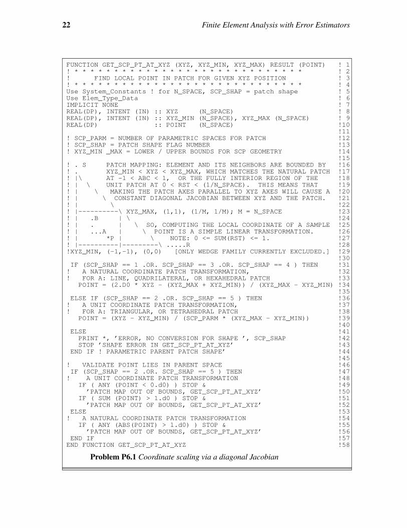
1.6 Problems from chapter 6Problem 6.1 Develop a function, say GET _SCP_PT _AT _XYZ , to find where an
element quadrature point or node is located within an element. Solution: As seen from
Fig. 6.2.1 the patch is nothing other than a single large parametric element designed to
have a constant diagonal Jacobian. That is, its sides or faces are generally constructed
parallel to the global axes. This assures that the inverse mapping from Ω to exists and
the non-dimensional coordinates, here POINT , are obtained as a linear scaling of the
global coordinates, XYZ . A typical function listing is given in P6.1.
Problem 6.2 Develop a routine, say EVAL_PT _FLUX_IN_SCP_PATCH , to
evaluate the flux components at any global coordinate point in a patch. Solution: A
typical source code is given in P6.2. Given the physical coordinates of a node the
previous function is first used to convert the location into a non-dimensional patch
parametric coordinate. Then the patch type, shape, parametric dimension, etc. are passed
to a general parametric interpolation routine, GEN_ELEM_SHAPE, that extracts a
matching element from the programs element interpolation library. Then those shape
functions are used to form the flux components at the local point. Those components are
scattered to the system nodes for later averaging. Each node that has received such a
scattered flux has a logical flag set so that some optional patch smoothing features can be
selected elsewhere to reduce the cost of the SCP fit.
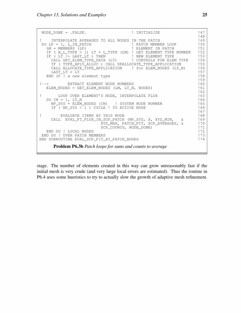
Problem 6.3 Employ the preceding patch routine to create a related subroutine, say
EVAL_SCP_FIT _AT _PATCH_NODES, that will interpolate patch fluxes back to all
mesh nodes inside the patch. Solution: These calculations are relatively simply. Most of
the routine involves setting up the interfaces, restricting the intended operations on the
arguments, and commenting on the variable names as seen in P6.3a. The actual loops, in
figure P6.3b, utilize the previous subroutine to scatter the continuous patch nodal flux
components to the system nodes and to update the contribution count for each node. As
seen in Chapter 6, these counts are then used to get a final averaged set of flux
components at each system node. They in turn are gathered at the element level to be
used in computing the error estimates and/or to compute system norms of interest.
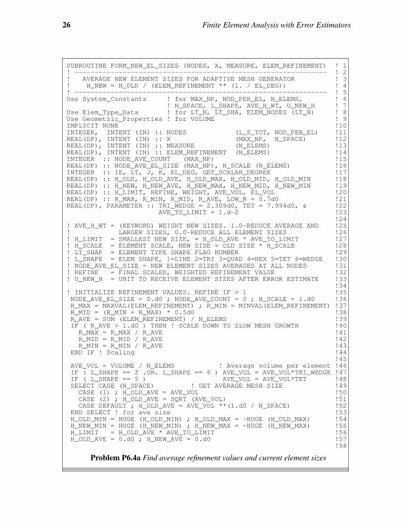
Problem 6.4 Develop a routine, say FORM_NEW_EL_SIZES, that can implement
the estimated new element sizes for an h-adaptivity based on Eqs. 5.28 and 29. Solution:
Most current mesh generators allow one to control the element sizes created by beginning
with a group of control points where you specify the desired element size at that point.
Here we simply use the desired element size, from the error estimator, averaged at each
node to be output to a file so that it can be read as input for the next mesh generation
22 Finite Element Analysis with Error Estimators
FUNCTION GET_SCP_PT_AT_XYZ (XYZ, XYZ_MIN, XYZ_MAX) RESULT (POINT) ! 1! * * * * * * * * * * * * * * * * * * * * * * * * * * * * * ! 2! FIND LOCAL POINT IN PATCH FOR GIVEN XYZ POSITION ! 3! * * * * * * * * * * * * * * * * * * * * * * * * * * * * * ! 4Use System_Constants ! for N_SPACE, SCP_SHAP = patch shape ! 5Use Elem_Type_Data ! 6IMPLICIT NONE ! 7REAL(DP), INTENT (IN) :: XYZ (N_SPACE) ! 8REAL(DP), INTENT (IN) :: XYZ_MIN (N_SPACE), XYZ_MAX (N_SPACE) ! 9REAL(DP) :: POINT (N_SPACE) !10
!11! SCP_PARM = NUMBER OF PARAMETRIC SPACES FOR PATCH !12! SCP_SHAP = PATCH SHAPE FLAG NUMBER !13! XYZ_MIN _MAX = LOWER / UPPER BOUNDS FOR SCP GEOMETRY !14
!15! . S PATCH MAPPING: ELEMENT AND ITS NEIGHBORS ARE BOUNDED BY !16! . XYZ_MIN < XYZ < XYZ_MAX, WHICH MATCHES THE NATURAL PATCH !17! |\ AT -1 < ABC < 1, OR THE FULLY INTERIOR REGION OF THE !18! | \ UNIT PATCH AT 0 < RST < (1/N_SPACE). THIS MEANS THAT !19! | \ MAKING THE PATCH AXES PARALLEL TO XYZ AXES WILL CAUSE A !20! | \ CONSTANT DIAGONAL JACOBIAN BETWEEN XYZ AND THE PATCH. !21! | \ !22! |----------\ XYZ_MAX, (1,1), (1/M, 1/M); M = N_SPACE !23! | .B | \ !24! | . | \ SO, COMPUTING THE LOCAL COORDINATE OF A SAMPLE !25! | ...A | \ POINT IS A SIMPLE LINEAR TRANSFORMATION. !26! | *P | \ NOTE: 0 <= SUM(RST) <= 1. !27! |----------|---------\ .....R !28!XYZ_MIN, (-1,-1), (0,0) [ONLY WEDGE FAMILY CURRENTLY EXCLUDED.] !29
!30IF (SCP_SHAP == 1 .OR. SCP_SHAP == 3 .OR. SCP_SHAP == 4 ) THEN !31
! A NATURAL COORDINATE PATCH TRANSFORMATION, !32! FOR A: LINE, QUADRILATERAL, OR HEXAHEDRAL PATCH !33
POINT = (2.D0 * XYZ - (XYZ_MAX + XYZ_MIN)) / (XYZ_MAX - XYZ_MIN) !34!35
ELSE IF (SCP_SHAP == 2 .OR. SCP_SHAP == 5 ) THEN !36! A UNIT COORDINATE PATCH TRANSFORMATION, !37! FOR A: TRIANGULAR, OR TETRAHEDRAL PATCH !38
POINT = (XYZ - XYZ_MIN) / (SCP_PARM * (XYZ_MAX - XYZ_MIN)) !39!40
ELSE !41PRINT *, ’ERROR, NO CONVERSION FOR SHAPE ’, SCP_SHAP !42STOP ’SHAPE ERROR IN GET_SCP_PT_AT_XYZ’ !43
END IF ! PARAMETRIC PARENT PATCH SHAPE’ !44!45
! VALIDATE POINT LIES IN PARENT SPACE !46IF (SCP_SHAP == 2 .OR. SCP_SHAP == 5 ) THEN !47
! A UNIT COORDINATE PATCH TRANSFORMATION !48IF ( ANY (POINT < 0.d0) ) STOP & !49
’PATCH MAP OUT OF BOUNDS, GET_SCP_PT_AT_XYZ’ !50IF ( SUM (POINT) > 1.d0 ) STOP & !51
’PATCH MAP OUT OF BOUNDS, GET_SCP_PT_AT_XYZ’ !52ELSE !53
! A NATURAL COORDINATE PATCH TRANSFORMATION !54IF ( ANY (ABS(POINT) > 1.d0) ) STOP & !55
’PATCH MAP OUT OF BOUNDS, GET_SCP_PT_AT_XYZ’ !56END IF !57
END FUNCTION GET_SCP_PT_AT_XYZ !58
Problem P6.1 Coordinate scaling via a diagonal Jacobian

Chapter 13, Solutions and Examples 23
SUBROUTINE EVAL_PT_FLUX_IN_SCP_PATCH (NP_SYS, X, XYZ_MIN, XYZ_MAX,& ! 1PATCH_FIT, SCP_AVERAGES, & ! 2SCP_COUNTS, NODE_DONE) ! 3
! * * * * * * * * * * * * * * * * * * * * * * * * * * * * * * * ! 4! CALCULATE THE SUPER_CONVERGENCE_PATCH FLUXES AT A NODE INSIDE ! 5! THE PATCH. (AVERAGE VALUES FROM ALL PATCHES LATER) ! 6! * * * * * * * * * * * * * * * * * * * * * * * * * * * * * * * ! 7Use System_Constants ! for MAX_NP, NEIGH_L, N_ELEMS, ! 8
! SCP_FIT, U_SCPR, N_SPACE ! 9Use Elem_Type_Data !10Use SCP_Type_Data ! for SCP_H (SCP_N) !11Use Interface_Header ! for function GET_SCP_PT_AT_XYZ !12IMPLICIT NONE !13INTEGER, INTENT (IN) :: NP_SYS ! CURRENT GLOBAL NODE !14REAL(DP), INTENT (IN) :: X (MAX_NP, N_SPACE) !15REAL(DP), INTENT (IN) :: XYZ_MIN (N_SPACE), XYZ_MAX (N_SPACE) !16REAL(DP), INTENT (IN) :: PATCH_FIT (SCP_N , N_R_B ) !17REAL(DP), INTENT (INOUT) :: SCP_AVERAGES (MAX_NP, SCP_FIT) !18INTEGER, INTENT (INOUT) :: SCP_COUNTS (MAX_NP) !19LOGICAL, INTENT (INOUT) :: NODE_DONE (MAX_NP) !20
!21REAL(DP) :: XYZ (N_SPACE), POINT (N_SPACE) ! SCP POINT !22REAL(DP) :: FLUX_PT (N_R_B) ! PT FLUX !23
!24INTEGER :: IS ! LOOPS !25INTEGER, PARAMETER :: ONE = 1 !26
!27! FLUX_PT = FLUX AT THE NODE INTERPOLATED FROM A SCP !28! MAX_NP = NUMBER OF SYSTEM NODES !29! NODE_DONE = TRUE, IF IT HAS ONE CONTRIBUTION FROM PATCH !30! NP_SYS = CURRENT GLOBAL NODE !31! PATCH_FIT = LOCAL PATCH VALUES FOR FLUX AT ITS NODES !32! POINT = LOCAL POINT IN PATCH INTERPOLATION SPACE !33! SCP_AVERAGES = AVERAGED FLUXES AT ALL NODES IN MESH !34! SCP_FIT = NUMBER OF TERMS BEING AVERAGED, = N_R_B MIN !35! SCP_H = INTERPOLATION FUNCTIONS FOR PATCH, USUALLY IS H !36! SCP_N = NUMBER OF NODES PER PATCH !37! X = COORDINATES OF SYSTEM NODES !38! XYZ = SPACE COORDINATES AT A POINT !39! XYZ_MAX = UPPER BOUNDS FOR SCP GEOMETRY !40! XYZ_MIN = LOWER BOUNDS FOR SCP GEOMETRY !41
!42! CONVERT IQ XYZ TO LOCAL PATCH POINT !43
XYZ = X (NP_SYS, :) !44POINT = GET_SCP_PT_AT_XYZ (XYZ, XYZ_MIN, XYZ_MAX) !45
!46! EVALUATE PATCH INTERPOLATION AT LOCAL POINT !47
CALL GEN_ELEM_SHAPE (POINT, SCP_H, SCP_N, N_SPACE, ONE) !48!49
! INTERPOLATE PATCH NODE FIT TO PHYSICAL NODE !50FLUX_PT (1:N_R_B) = MATMUL (SCP_H (:), PATCH_FIT (:, 1:N_R_B)) !51
!52! SCATTER NODE VALUES TO SYSTEM & INCREMENT COUNTS !53
SCP_COUNTS (NP_SYS) = SCP_COUNTS (NP_SYS) + 1 !54SCP_AVERAGES (NP_SYS, 1:N_R_B) = SCP_AVERAGES (NP_SYS, 1:N_R_B) & !55
+ FLUX_PT (1:N_R_B) !56NODE_DONE (NP_SYS) = .TRUE. !57
END SUBROUTINE EVAL_PT_FLUX_IN_SCP_PATCH !58
Problem P6.2 Computing and scattering flux components at a node

24 Finite Element Analysis with Error Estimators
SUBROUTINE EVAL_SCP_FIT_AT_PATCH_NODES (IP, NODES, X, L_IN_PATCH, &! 1MEMBERS, XYZ_MIN, XYZ_MAX, PATCH_FIT, &! 2SCP_AVERAGES, SCP_COUNTS) ! 3
! * * * * * * * * * * * * * * * * * * * * * * * * * * * * * * * ! 4! CALCULATE THE SUPER_CONVERGENCE_PATCH AVERAGE FLUXES ! 5! AT ALL ELEMENT NODES INSIDE THE PATCH ! 6! * * * * * * * * * * * * * * * * * * * * * * * * * * * * * * * ! 7Use System_Constants ! for MAX_NP, N_ELEMS, L_S_TOT, N_SPACE, ! 8
! SCP_FIT, SCP_N , N_R_B ! 9Use Elem_Type_Data ! for ELEM_NODES, LAST_LT, LT_* !10Use Interface_Header ! for GET_ELEM_NODES function !11IMPLICIT NONE !12INTEGER, INTENT (IN) :: IP ! CURRENT PATCH NUMBER !13INTEGER, INTENT (IN) :: NODES (L_S_TOT, NOD_PER_EL) !14REAL(DP), INTENT (IN) :: X (MAX_NP, N_SPACE) !15INTEGER, INTENT (IN) :: L_IN_PATCH !16INTEGER, INTENT (IN) :: MEMBERS (L_IN_PATCH) !17REAL(DP), INTENT (IN) :: XYZ_MIN (N_SPACE), XYZ_MAX (N_SPACE) !18REAL(DP), INTENT (IN) :: PATCH_FIT (SCP_N , N_R_B ) !19REAL(DP), INTENT (INOUT) :: SCP_AVERAGES (MAX_NP, SCP_FIT) !20INTEGER, INTENT (INOUT) :: SCP_COUNTS (MAX_NP) !21
!22INTEGER :: IN, LM, LP, LT, NP_SYS ! LOOPS !23LOGICAL :: NODE_DONE (MAX_NP) !24
!25! ELEM_NODES = THE NOD_PER_EL INCIDENCES OF THE ELEMENT !26! IP = CURRENT PATCH NUMBER !27! L_IN_PATCH = NUMBER OF ELEMENTS IN CURRENT SCP !28! L_S_TOT = TOTAL NUMBER OF ELEMENTS & THEIR SEGMENTS !29! L_TYPE = ELEMENT TYPE NUMBER FOR ALL ELEMENTS !30! LAST_LT = LAST ELEMENT TYPE CREATED !31! LT = CURRENT ELEMENT TYPE NUMBER !32! LT_N = MAXIMUM NUMBER OF NODES FOR ELEMENT TYPE !33! MAX_NP = NUMBER OF SYSTEM NODES !34! MEMBERS = ELEMENT NUMBERS MACKING UP A SCP !35! NOD_PER_EL = MAXIMUM NUMBER OF NODES PER ELEMENT !36! NODES = NODAL INCIDENCES OF ALL ELEMENTS !37! NODE_DONE = TRUE, IF IT HAS ONE CONTRIBUTION FROM PATCH !38! N_SPACE = DIMENSION OF SPACE !39! PATCH_FIT = LOCAL PATCH VALUES FOR FLUX AT ITS NODES !40! SCP_AVERAGES = AVERAGED FLUXES AT ALL NODES IN MESH !41! SCP_FIT = NUMBER IF TERMS BEING AVERAGED, = N_R_B MIN !42! X = COORDINATES OF SYSTEM NODES !43! XYZ_MAX = UPPER BOUNDS FOR SCP GEOMETRY !44! XYZ_MIN = LOWER BOUNDS FOR SCP GEOMETRY !45
!46
Problem P6.3a Establishing the interface for continuous flux scatters
Chapter 13, Solutions and Examples 25
NODE_DONE = .FALSE. ! INITIALIZE !47!48
! INTERPOLATE AVERAGES TO ALL NODES IN THE PATCH !49DO LP = 1, L_IN_PATCH ! PATCH MEMBER LOOP !50
LM = MEMBERS (LP) ! ELEMENT IN PATCH !51IF ( N_L_TYPE > 1) LT = L_TYPE (LM) ! GET ELEMENT TYPE NUMBER !52IF ( LT /= LAST_LT ) THEN ! NEW ELEMENT TYPE !53
CALL GET_ELEM_TYPE_DATA (LT) ! CONTROLS FOR ELEM TYPE !54IF ( TYPE_APLY_ALLOC ) CALL DEALLOCATE_TYPE_APPLICATION !55CALL ALLOCATE_TYPE_APPLICATION ! for ELEM_NODES (LT_N) !56LAST_LT = LT !57
END IF ! a new element type !58!59
!--> EXTRACT ELEMENT NODE NUMBERS !60ELEM_NODES = GET_ELEM_NODES (LM, LT_N, NODES) !61
!62! LOOP OVER ELEMENT’S NODE, INTERPOLATE FLUX !63
DO IN = 1, LT_N !64NP_SYS = ELEM_NODES (IN) ! SYSTEM NODE NUMBER !65IF ( NP_SYS < 1 ) CYCLE ! TO ACTIVE NODE !66
!67! EVALUATE ITEMS AT THIS NODE !68
CALL EVAL_PT_FLUX_IN_SCP_PATCH (NP_SYS, X, XYZ_MIN, & !69XYZ_MAX, PATCH_FIT, SCP_AVERAGES, & !70SCP_COUNTS, NODE_DONE) !71
END DO ! LOCAL NODES !72END DO ! OVER PATCH MEMBERS !73
END SUBROUTINE EVAL_SCP_FIT_AT_PATCH_NODES !74
Problem P6.3b Patch loops for sums and counts to average
stage. The number of elements created in this way can grow unreasonably fast if the
initial mesh is very crude (and very large local errors are estimated). Thus the routine in
P6.4 uses some hueristics to try to actually slow the growth of adaptive mesh refinement.
26 Finite Element Analysis with Error Estimators
SUBROUTINE FORM_NEW_EL_SIZES (NODES, X, MEASURE, ELEM_REFINEMENT) ! 1! --------------------------------------------------------------- ! 2! AVERAGE NEW ELEMENT SIZES FOR ADAPTIVE MESH GENERATOR ! 3! H_NEW = H_OLD / (ELEM_REFINEMENT ** (1. / EL_DEG)) ! 4! --------------------------------------------------------------- ! 5Use System_Constants ! for MAX_NP, NOD_PER_EL, N_ELEMS, ! 6
! N_SPACE, L_SHAPE, AVE_H_WT, U_NEW_H ! 7Use Elem_Type_Data ! for LT_N, LT_SHA, ELEM_NODES (LT_N) ! 8Use Geometric_Properties ! for VOLUME ! 9IMPLICIT NONE !10INTEGER, INTENT (IN) :: NODES (L_S_TOT, NOD_PER_EL) !11REAL(DP), INTENT (IN) :: X (MAX_NP, N_SPACE) !12REAL(DP), INTENT (IN) :: MEASURE (N_ELEMS) !13REAL(DP), INTENT (IN) :: ELEM_REFINEMENT (N_ELEMS) !14INTEGER :: NODE_AVE_COUNT (MAX_NP) !15REAL(DP) :: NODE_AVE_EL_SIZE (MAX_NP), H_SCALE (N_ELEMS) !16INTEGER :: IE, LT, J, K, EL_DEG, GET_SCALAR_DEGREE !17REAL(DP) :: H_OLD, H_OLD_AVE, H_OLD_MAX, H_OLD_MID, H_OLD_MIN !18REAL(DP) :: H_NEW, H_NEW_AVE, H_NEW_MAX, H_NEW_MID, H_NEW_MIN !19REAL(DP) :: H_LIMIT, REFINE, WEIGHT, AVE_VOL, EL_VOL !20REAL(DP) :: R_MAX, R_MIN, R_MID, R_AVE, LOW_R = 0.7d0 !21REAL(DP), PARAMETER :: TRI_WEDGE = 2.309d0, TET = 7.994d0, & !22
AVE_TO_LIMIT = 1.d-2 !23!24
! AVE_H_WT = (KEYWORD) WEIGHT NEW SIZES. 1.0-REDUCE AVERAGE AND !25! LARGER SIZES, 0.0-REDUCE ALL ELEMENT SIZES !26! H_LIMIT = SMALLEST NEW SIZE, = H_OLD_AVE * AVE_TO_LIMIT !27! H_SCALE = ELEMENT SCALE, NEW SIZE = OLD SIZE * H_SCALE !28! LT_SHAP = ELEMENT TYPE SHAPE FLAG NUMBER !29! L_SHAPE = ELEM SHAPE, 1=LINE 2=TRI 3=QUAD 4=HEX 5=TET 6=WEDGE !30! NODE_AVE_EL_SIZE = NEW ELEMENT SIZES AVERAGED AT ALL NODES !31! REFINE = FINAL SCALED, WEIGHTED REFINEMENT VALUE !32! U_NEW_H = UNIT TO RECEIVE ELEMENT SIZES AFTER ERROR ESTIMATE !33
!34! INITIALIZE REFINEMENT VALUES. REFINE IF > 1 !35NODE_AVE_EL_SIZE = 0.d0 ; NODE_AVE_COUNT = 0 ; H_SCALE = 1.d0 !36R_MAX = MAXVAL(ELEM_REFINEMENT) ; R_MIN = MINVAL(ELEM_REFINEMENT) !37R_MID = (R_MIN + R_MAX) * 0.5d0 !38R_AVE = SUM (ELEM_REFINEMENT) / N_ELEMS !39IF ( R_AVE > 1.d0 ) THEN ! SCALE DOWN TO SLOW MESH GROWTH !40
R_MAX = R_MAX / R_AVE !41R_MID = R_MID / R_AVE !42R_MIN = R_MIN / R_AVE !43
END IF ! Scaling !44!45
AVE_VOL = VOLUME / N_ELEMS ! Average volume per element !46IF ( L_SHAPE == 2 .OR. L_SHAPE == 6 ) AVE_VOL = AVE_VOL*TRI_WEDGE !47IF ( L_SHAPE == 5 ) AVE_VOL = AVE_VOL*TET !48SELECT CASE (N_SPACE) ! GET AVERAGE MESH SIZE !49
CASE (1) ; H_OLD_AVE = AVE_VOL !50CASE (2) ; H_OLD_AVE = SQRT (AVE_VOL) !51CASE DEFAULT ; H_OLD_AVE = AVE_VOL **(1.d0 / N_SPACE) !52
END SELECT ! for ave size !53H_OLD_MIN = HUGE (H_OLD_MIN) ; H_OLD_MAX = -HUGE (H_OLD_MAX) !54H_NEW_MIN = HUGE (H_NEW_MIN) ; H_NEW_MAX = -HUGE (H_NEW_MAX) !55H_LIMIT = H_OLD_AVE * AVE_TO_LIMIT !56H_OLD_AVE = 0.d0 ; H_NEW_AVE = 0.d0 !57
!58
Problem P6.4a Find average refinement values and current element sizes

Chapter 13, Solutions and Examples 27
! LOOP OVER ALL STANDARD ELEMENTS ! 59LT = 1 ; LAST_LT = 0 ! 60DO IE = 1, N_ELEMS ! LOOP OVER ALL ELEMENTS ------------------ ! 61
CALL SET_THIS_ELEMENT_NUMBER (IE) ! 62! 63
!--> GET ELEMENT TYPE NUMBER ! 64IF ( N_L_TYPE > 1) LT = L_TYPE (IE) ! SAME AS LAST TYPE ? ! 65IF ( LT /= LAST_LT ) THEN ! this is a new type ! 66
CALL GET_ELEM_TYPE_DATA (LT) ! CONTROLS FOR THIS TYPE ! 67LAST_LT = LT ! 68IF ( TYPE_APLY_ALLOC ) CALL DEALLOCATE_TYPE_APPLICATION ! 69CALL ALLOCATE_TYPE_APPLICATION ! for ELEM_NODES (LT_N) ! 70EL_DEG = GET_SCALAR_DEGREE () ! 71
END IF ! a new element type ! 72! 73
! GET AVERAGE ELEMENT SIZE (or recompute its volume) ! 74EL_VOL = MEASURE (IE) ! 75IF ( LT_SHAP == 2 .OR. LT_SHAP == 6 ) EL_VOL=EL_VOL*TRI_WEDGE ! 76IF ( LT_SHAP == 5 ) EL_VOL=EL_VOL*TET ! 77SELECT CASE (N_SPACE) ! 78
CASE (1) ; H_OLD = EL_VOL ! 79CASE (2) ; H_OLD = SQRT (EL_VOL) ! 80CASE DEFAULT ; H_OLD = EL_VOL **(1.d0 / N_SPACE) ! 81
END SELECT ! for old size ! 82H_OLD_AVE = H_OLD_AVE + H_OLD ! 83IF ( H_OLD > H_OLD_MAX ) H_OLD_MAX = H_OLD ! 84IF ( H_OLD < H_OLD_MIN ) H_OLD_MIN = H_OLD ! 85
! 86! GET NEW ELEMENT SIZE, WEIGHT TO CONTROL GROWTH ! 87
WEIGHT = R_MIN * (1.d0 - AVE_H_WT) + R_AVE * AVE_H_WT ! 88REFINE = ELEM_REFINEMENT (IE) / WEIGHT ! 89IF ( REFINE > LOW_R ) THEN ! 90
SELECT CASE (EL_DEG) ! 91CASE (1) ; H_SCALE (IE) = 1.d0 / REFINE ! 92CASE (2) ; H_SCALE (IE) = 1.d0 / SQRT (REFINE) ! 93CASE DEFAULT ; H_SCALE (IE) = 1.d0/REFINE **(1.d0/EL_DEG) ! 94
END SELECT ! 95END IF ! reduce size (no increases) ! 96H_NEW = H_OLD * H_SCALE (IE) ! 97IF ( H_NEW < H_LIMIT ) H_NEW = H_LIMIT ! 98IF ( H_NEW > H_NEW_MAX ) H_NEW_MAX = H_NEW ! 99IF ( H_NEW < H_NEW_MIN ) H_NEW_MIN = H_NEW !100H_NEW_AVE = H_NEW_AVE + H_NEW !101
!102! SEND SIZES FOR AVERAGING AT NODES !103
ELEM_NODES = GET_ELEM_NODES (IE, LT_N, NODES) !104DO J = 1, LT_N !105
K = ELEM_NODES (J) !106IF ( K < 1 ) CYCLE ! to a valid node !107
NODE_AVE_EL_SIZE (K) = NODE_AVE_EL_SIZE (K) + H_NEW !108NODE_AVE_COUNT (K) = NODE_AVE_COUNT (K) + 1 !109
END DO ! over element nodes !110END DO ! over elements ---------------------------------------- !111
Problem P6.4b Get each new element size and scatter to its nodes

28 Finite Element Analysis with Error Estimators
H_OLD_AVE = H_OLD_AVE / N_ELEMS !112H_NEW_AVE = H_NEW_AVE / N_ELEMS !113H_NEW_MID = (H_NEW_MIN + H_NEW_MAX) * 0.5d0 !114H_OLD_MID = (H_OLD_MIN + H_OLD_MAX) * 0.5d0 !115
!116! AVERAGE SIZES AT NODES FOR MESH GENERATOR !117WHERE ( NODE_AVE_COUNT > 0 ) !118
NODE_AVE_EL_SIZE = NODE_AVE_EL_SIZE / NODE_AVE_COUNT !119ELSEWHERE !120
NODE_AVE_EL_SIZE = H_NEW_AVE !121ENDWHERE !122
!123! SAVE RESULTS FOR PLOTS AND/OR MESH GENERATOR !124WRITE (U_NEW_H, ’(5I12)’) MAX_NP, (K, K = 1, N_SPACE) ! for plot !125DO J = 1, MAX_NP ! save averaged sizes at nodes !126
WRITE (U_NEW_H, ’(3(1PE12.4))’) X (J, :), NODE_AVE_EL_SIZE (J) !127END DO ! over nodes !128
END SUBROUTINE FORM_NEW_EL_SIZES !129
Problem P6.4c Average all element sizes at mesh nodes and save
1.7 Problems from chapter 7
Problem 7.10 Resolve the heat transfer problem in Fig. 7.7.1 with the external
reference temperature increased from 0 to 20 F (U_ext = 20). Employ 3 equal length L2
linear elements, and 5 (not 4) nodes with nodes 2 and 3 both at x = 4/3. Connect
element 1 to nodes 1 and 2 and (incorrectly) connect element 2 to nodes 3 and 4. a) Solve
the incorrect model, sketch the FEA and true solutions, and discuss why the left and right
(x ≤ 4/3 and x ≥ 4/3) domain FEA solutions behave as they do. b) Enforce the correct
solution by imposing a so called "multiple point constraint" (MPC) that requires
1 × t2 − 1 × t3 = 0. Solution: (a) This only requires changing the data in Fig.7.7.3, as
described above, and applying the matrix definitions in Fig. 7.7.2, or the simplified L2
version thereof. The invalid (discontinuous) FEA solution is given in P7.10a.
Solution: b) One must either correct the mesh to have the proper connectivity, or
apply a MPC to enforce continuity. Here the latter is employed to reinforce the concept of
MPC’s which are often needed in real applications to correct data errors (as here) or for
other analysis reasons. The corrected solution is in P7.10b and is reasonable for a 3
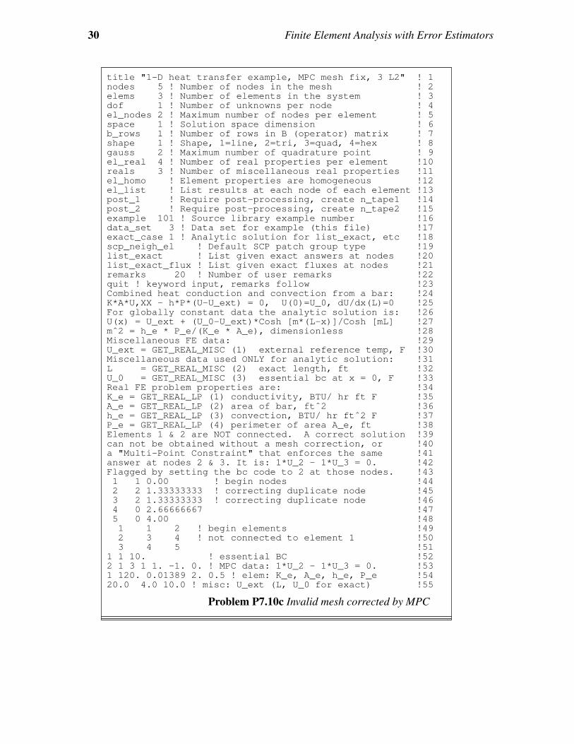
element solution. The data for this solution are given in P7.10c. In the MODEL code a
MPC between 2 degrees of freedom is referred to as a "Type 2" constraint. In lines 45
and 46 of P7.10c the normally zero boundary constraint flag has been set to 2 for each of
the constrained degrees of freedom. For each such pair of flags there must be one "Type
2" constraint equation. In general its form would be a × t j + b × tk = c. Here we want 2
dof to be identical so we set a = 1, b = − 1, c = 0. In addition we must provide the
equation numbers, j and k. Here j is for node 2, parameter 1, while k is for node 3, and
also parameter 1. Those data are give after the essential boundary conditions (the "Type
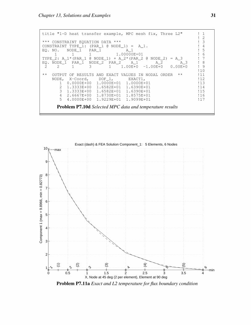
1" conditions) and appear at line 53 of the data set. The selected output in P7.10d echos
these constraint data again and gives the FEA and exact nodal values.
Problem 7.11 Implement the exact integral matrices for the linear line element version of
Eq. 7.34 and the matrix for recovering the convection heat loss, Eq. 7.38, in the post

Chapter 13, Solutions and Examples 29
0 0.5 1 1.5 2 2.5 3 3.5 410
11
12
13
14
15
16
17
18
19
20
X, Node at 45 deg (2 per element), Element at 90 deg
Exact (dash) & FEA Solution Component_1: 3 Elements, 5 Nodes
Com
pone
nt 1
(m
ax =
20,
min
= 1
0)
(1
)
(2
)
(3
)
1
2
3
4
5
−−−min
−−−max
Invalid mesh without MPC
Nodes 2 and 3 have same x coordinate
Problem P7.10a Invalid (discontinuous) L2 convection solution results
0 0.5 1 1.5 2 2.5 3 3.5 410
11
12
13
14
15
16
17
18
19
X, Node at 45 deg (2 per element), Element at 90 deg
Exact (dash) & FEA Solution Component_1: 3 Elements, 5 Nodes
Com
pone
nt 1
(m
ax =
19.
2294
, min
= 1
0)
(1
)
(2
)
(3
)
1
2
3
4
5
−−−min
−−−max
Problem P7.10b Corrected (via MPC) L2 convection solution results
30 Finite Element Analysis with Error Estimators
title "1-D heat transfer example, MPC mesh fix, 3 L2" ! 1nodes 5 ! Number of nodes in the mesh ! 2elems 3 ! Number of elements in the system ! 3dof 1 ! Number of unknowns per node ! 4el_nodes 2 ! Maximum number of nodes per element ! 5space 1 ! Solution space dimension ! 6b_rows 1 ! Number of rows in B (operator) matrix ! 7shape 1 ! Shape, 1=line, 2=tri, 3=quad, 4=hex ! 8gauss 2 ! Maximum number of quadrature point ! 9el_real 4 ! Number of real properties per element !10reals 3 ! Number of miscellaneous real properties !11el_homo ! Element properties are homogeneous !12el_list ! List results at each node of each element !13post_1 ! Require post-processing, create n_tape1 !14post_2 ! Require post-processing, create n_tape2 !15example 101 ! Source library example number !16data_set 3 ! Data set for example (this file) !17exact_case 1 ! Analytic solution for list_exact, etc !18scp_neigh_el ! Default SCP patch group type !19list_exact ! List given exact answers at nodes !20list_exact_flux ! List given exact fluxes at nodes !21remarks 20 ! Number of user remarks !22quit ! keyword input, remarks follow !23Combined heat conduction and convection from a bar: !24K*A*U,XX - h*P*(U-U_ext) = 0, U(0)=U_0, dU/dx(L)=0 !25For globally constant data the analytic solution is: !26U(x) = U_ext + (U_0-U_ext)*Cosh [m*(L-x)]/Cosh [mL] !27mˆ2 = h_e * P_e/(K_e * A_e), dimensionless !28Miscellaneous FE data: !29U_ext = GET_REAL_MISC (1) external reference temp, F !30Miscellaneous data used ONLY for analytic solution: !31L = GET_REAL_MISC (2) exact length, ft !32U_0 = GET_REAL_MISC (3) essential bc at x = 0, F !33Real FE problem properties are: !34K_e = GET_REAL_LP (1) conductivity, BTU/ hr ft F !35A_e = GET_REAL_LP (2) area of bar, ftˆ2 !36h_e = GET_REAL_LP (3) convection, BTU/ hr ftˆ2 F !37P_e = GET_REAL_LP (4) perimeter of area A_e, ft !38Elements 1 & 2 are NOT connected. A correct solution !39can not be obtained without a mesh correction, or !40a "Multi-Point Constraint" that enforces the same !41answer at nodes 2 & 3. It is: 1*U_2 - 1*U_3 = 0. !42Flagged by setting the bc code to 2 at those nodes. !431 1 0.00 ! begin nodes !442 2 1.33333333 ! correcting duplicate node !453 2 1.33333333 ! correcting duplicate node !464 0 2.66666667 !475 0 4.00 !481 1 2 ! begin elements !492 3 4 ! not connected to element 1 !503 4 5 !51
1 1 10. ! essential BC !522 1 3 1 1. -1. 0. ! MPC data: 1*U_2 - 1*U_3 = 0. !531 120. 0.01389 2. 0.5 ! elem: K_e, A_e, h_e, P_e !5420.0 4.0 10.0 ! misc: U_ext (L, U_0 for exact) !55
Problem P7.10c Invalid mesh corrected by MPC
Chapter 13, Solutions and Examples 31
title "1-D heat transfer example, MPC mesh fix, Three L2" ! 1! 2
*** CONSTRAINT EQUATION DATA *** ! 3CONSTRAINT TYPE_1: (PAR_1 @ NODE_1) = A_1. ! 4EQ. NO. NODE_1 PAR_1 A_1 ! 5
1 1 1 1.00000E+01 ! 6TYPE_2: A_1*(PAR_1 @ NODE_1) + A_2*(PAR_2 @ NODE_2) = A_3 ! 7EQ. NODE_1 PAR_1 NODE_2 PAR_2 A_1 A_2 A_3 ! 82 2 1 3 1 1.00E+0 -1.00E+0 0.00E+0 ! 9
!10** OUTPUT OF RESULTS AND EXACT VALUES IN NODAL ORDER ** !11
NODE, X-Coord, DOF_1, EXACT1, !121 0.0000E+00 1.0000E+01 1.0000E+01 !132 1.3333E+00 1.6582E+01 1.6390E+01 !143 1.3333E+00 1.6582E+01 1.6390E+01 !154 2.6667E+00 1.8730E+01 1.8575E+01 !165 4.0000E+00 1.9229E+01 1.9099E+01 !17
Problem P7.10d Selected MPC data and temperature results
0 0.5 1 1.5 2 2.5 3 3.5 4
1
2
3
4
5
6
7
8
9
10
X, Node at 45 deg (2 per element), Element at 90 deg
Exact (dash) & FEA Solution Component_1: 5 Elements, 6 Nodes
Com
pone
nt 1
(m
ax =
9.8
966,
min
= 0
.827
73)
(1
)
(2
)
(3
)
(4
)
(5
)
1
2
3
4
5
6
−−−min
−−−max
Problem P7.11a Exact and L2 temperature for flux boundary condition
32 Finite Element Analysis with Error Estimators
processing. Apply a small model to the problem in Fig. 7.7.1, but replace the Dirichlet
boundary condition at x = 0 with the corresponding exact flux q(0) = 12. 86. Compare
the temperature solution with that in Fig. 7.7.1. Why do we still get a solution when we
no longer have a Dirichlet boundary condition? Solution: The definitions of the matrices
are given in the text for the L2 element. Here we have simply multiplied the constant
element coefficients times arrays defined with the F90 RESHAPE intrinsic to convert the
vector data, stored by columns, into a matrix of the desired shape. One additional change
is that we follow the usual practice here and assume that the external reference
temperature can be different for each element. It is element real property number 5 here.
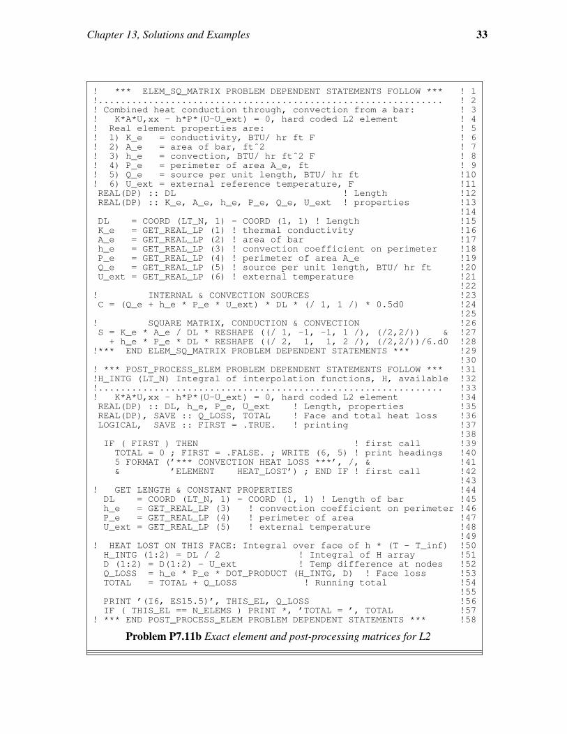
Selected results are compared in P7.11a. The element matrices are in P7.11b for
both the element generation and post-processing phases. The latter involves the integral
of the solution.
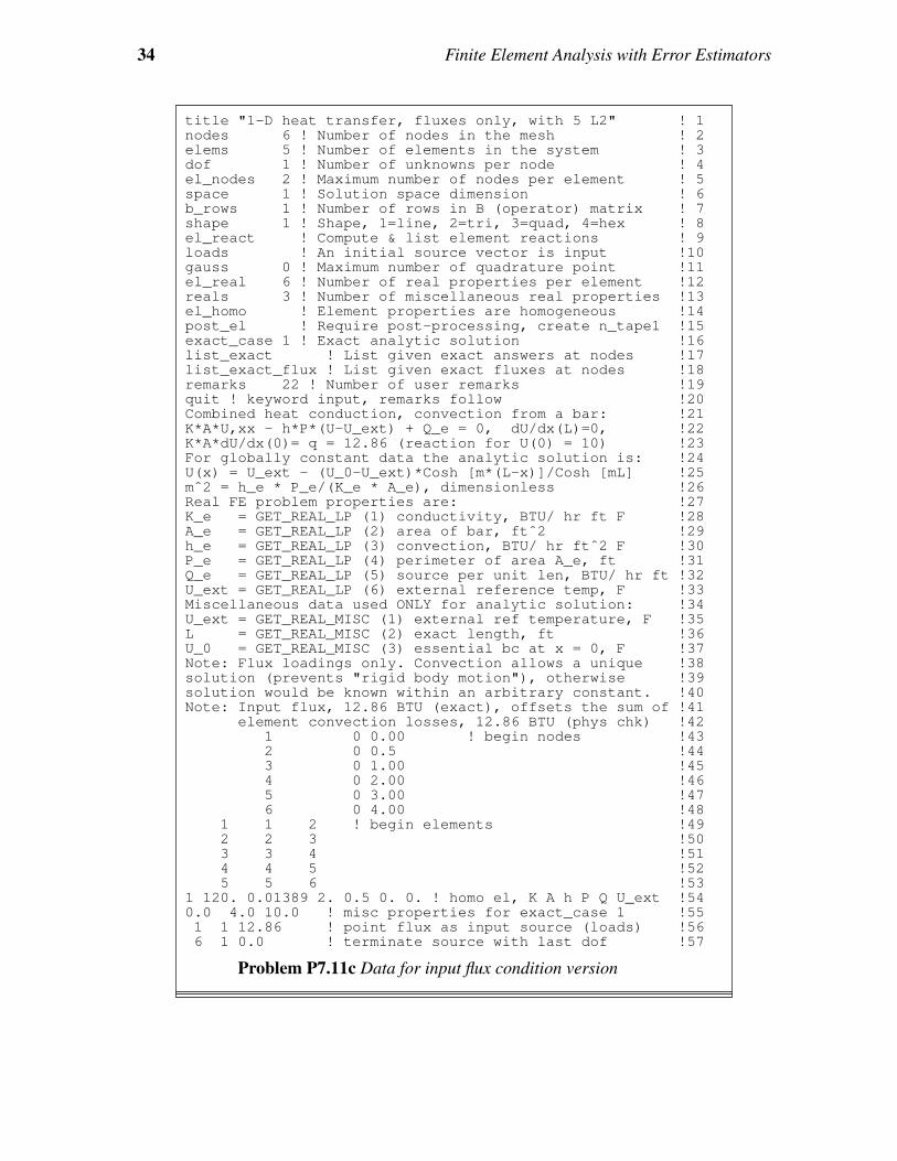
A set of sample data for this element and a flux boundary condition is given in
P7.11c. The assigned flux (computed from the exact flux at x = 0) is noted in lines 10
and 56. The remarks, lines 38 to 40, address why we can get a unique solution without a
Dirichlet boundary condition. Selected output from these data are in P7.11d. It is very
unusual for a problem not to have at least one Dirichlet boundary condition so a warning
is observed on line 3. The input flux data is echoed in line 7. As expected its value is
equal and opposite to the convection heat loss listed in lines 50 to 57. The computed
temperatures are reasonably accurate. Note that the value at x = 0 is in error by one
percent compared to the Dirichlet boundary condition value used to compute the exact
solution. That is mainly due to weak form implementation of the insulated condition at
the right end of the bar (x = 4).
In lines 23 to 48 of P7.11d we see the element level reactions, which represent heat
flows. These data were requested in line 9 of P7.11c. Since those reactions are not equal
and opposite to each other there must have been an internal heat source per unit length
and/or a surface convection heat loss. In this case their differences, cited in the rightmost
SUMS column, should equal the heat flow lost from each element by convection. That is
confirmed again bu looking at lines 50 to 57. Normally we do not look at such element
reactions in detail but they can be important in applications like heat transfer and
structural mechanics.
1.8 Problems from chapter 8
Problem 8.1 A hollow coaxial cable is made from a hollow conducting core and an
insulating outer layer with ε 1 = 0. 5, ε 2 = 2. 0 and charge densities of ζ 1 = 100 and ζ 2 = 0,
respectively. The inner, interface, and outer radii are 5, 10, and 25 mm. The
corresponding inner and outer potentials (boundary conditions) are φ = 500 and φ = 0,
respectively. Use the element formulation in Fig. 8.2.1 to compute the interface potential.
Solution: The element definition in Fig. 8.3.2 will work for all C0 line elements in the
library. We just need a new data file since the differential equation is the same. Data and
results for 2 cubic line elements are in P8.1
Chapter 13, Solutions and Examples 33
! *** ELEM_SQ_MATRIX PROBLEM DEPENDENT STATEMENTS FOLLOW *** ! 1!.............................................................. ! 2! Combined heat conduction through, convection from a bar: ! 3! K*A*U,xx - h*P*(U-U_ext) = 0, hard coded L2 element ! 4! Real element properties are: ! 5! 1) K_e = conductivity, BTU/ hr ft F ! 6! 2) A_e = area of bar, ftˆ2 ! 7! 3) h_e = convection, BTU/ hr ftˆ2 F ! 8! 4) P_e = perimeter of area A_e, ft ! 9! 5) Q_e = source per unit length, BTU/ hr ft !10! 6) U_ext = external reference temperature, F !11REAL(DP) :: DL ! Length !12REAL(DP) :: K_e, A_e, h_e, P_e, Q_e, U_ext ! properties !13
!14DL = COORD (LT_N, 1) - COORD (1, 1) ! Length !15K_e = GET_REAL_LP (1) ! thermal conductivity !16A_e = GET_REAL_LP (2) ! area of bar !17h_e = GET_REAL_LP (3) ! convection coefficient on perimeter !18P_e = GET_REAL_LP (4) ! perimeter of area A_e !19Q_e = GET_REAL_LP (5) ! source per unit length, BTU/ hr ft !20U_ext = GET_REAL_LP (6) ! external temperature !21
!22! INTERNAL & CONVECTION SOURCES !23C = (Q_e + h_e * P_e * U_ext) * DL * (/ 1, 1 /) * 0.5d0 !24
!25! SQUARE MATRIX, CONDUCTION & CONVECTION !26S = K_e * A_e / DL * RESHAPE ((/ 1, -1, -1, 1 /), (/2,2/)) & !27
+ h_e * P_e * DL * RESHAPE ((/ 2, 1, 1, 2 /), (/2,2/))/6.d0 !28!*** END ELEM_SQ_MATRIX PROBLEM DEPENDENT STATEMENTS *** !29
!30! *** POST_PROCESS_ELEM PROBLEM DEPENDENT STATEMENTS FOLLOW *** !31!H_INTG (LT_N) Integral of interpolation functions, H, available !32!.............................................................. !33! K*A*U,xx - h*P*(U-U_ext) = 0, hard coded L2 element !34REAL(DP) :: DL, h_e, P_e, U_ext ! Length, properties !35REAL(DP), SAVE :: Q_LOSS, TOTAL ! Face and total heat loss !36LOGICAL, SAVE :: FIRST = .TRUE. ! printing !37
!38IF ( FIRST ) THEN ! first call !39
TOTAL = 0 ; FIRST = .FALSE. ; WRITE (6, 5) ! print headings !405 FORMAT (’*** CONVECTION HEAT LOSS ***’, /, & !41& ’ELEMENT HEAT_LOST’) ; END IF ! first call !42
!43! GET LENGTH & CONSTANT PROPERTIES !44
DL = COORD (LT_N, 1) - COORD (1, 1) ! Length of bar !45h_e = GET_REAL_LP (3) ! convection coefficient on perimeter !46P_e = GET_REAL_LP (4) ! perimeter of area !47U_ext = GET_REAL_LP (5) ! external temperature !48
!49! HEAT LOST ON THIS FACE: Integral over face of h * (T - T_inf) !50
H_INTG (1:2) = DL / 2 ! Integral of H array !51D (1:2) = D(1:2) - U_ext ! Temp difference at nodes !52Q_LOSS = h_e * P_e * DOT_PRODUCT (H_INTG, D) ! Face loss !53TOTAL = TOTAL + Q_LOSS ! Running total !54
!55PRINT ’(I6, ES15.5)’, THIS_EL, Q_LOSS !56IF ( THIS_EL == N_ELEMS ) PRINT *, ’TOTAL = ’, TOTAL !57
! *** END POST_PROCESS_ELEM PROBLEM DEPENDENT STATEMENTS *** !58
Problem P7.11b Exact element and post-processing matrices for L2
34 Finite Element Analysis with Error Estimators
title "1-D heat transfer, fluxes only, with 5 L2" ! 1nodes 6 ! Number of nodes in the mesh ! 2elems 5 ! Number of elements in the system ! 3dof 1 ! Number of unknowns per node ! 4el_nodes 2 ! Maximum number of nodes per element ! 5space 1 ! Solution space dimension ! 6b_rows 1 ! Number of rows in B (operator) matrix ! 7shape 1 ! Shape, 1=line, 2=tri, 3=quad, 4=hex ! 8el_react ! Compute & list element reactions ! 9loads ! An initial source vector is input !10gauss 0 ! Maximum number of quadrature point !11el_real 6 ! Number of real properties per element !12reals 3 ! Number of miscellaneous real properties !13el_homo ! Element properties are homogeneous !14post_el ! Require post-processing, create n_tape1 !15exact_case 1 ! Exact analytic solution !16list_exact ! List given exact answers at nodes !17list_exact_flux ! List given exact fluxes at nodes !18remarks 22 ! Number of user remarks !19quit ! keyword input, remarks follow !20Combined heat conduction, convection from a bar: !21K*A*U,xx - h*P*(U-U_ext) + Q_e = 0, dU/dx(L)=0, !22K*A*dU/dx(0)= q = 12.86 (reaction for U(0) = 10) !23For globally constant data the analytic solution is: !24U(x) = U_ext - (U_0-U_ext)*Cosh [m*(L-x)]/Cosh [mL] !25mˆ2 = h_e * P_e/(K_e * A_e), dimensionless !26Real FE problem properties are: !27K_e = GET_REAL_LP (1) conductivity, BTU/ hr ft F !28A_e = GET_REAL_LP (2) area of bar, ftˆ2 !29h_e = GET_REAL_LP (3) convection, BTU/ hr ftˆ2 F !30P_e = GET_REAL_LP (4) perimeter of area A_e, ft !31Q_e = GET_REAL_LP (5) source per unit len, BTU/ hr ft !32U_ext = GET_REAL_LP (6) external reference temp, F !33Miscellaneous data used ONLY for analytic solution: !34U_ext = GET_REAL_MISC (1) external ref temperature, F !35L = GET_REAL_MISC (2) exact length, ft !36U_0 = GET_REAL_MISC (3) essential bc at x = 0, F !37Note: Flux loadings only. Convection allows a unique !38solution (prevents "rigid body motion"), otherwise !39solution would be known within an arbitrary constant. !40Note: Input flux, 12.86 BTU (exact), offsets the sum of !41
element convection losses, 12.86 BTU (phys chk) !421 0 0.00 ! begin nodes !432 0 0.5 !443 0 1.00 !454 0 2.00 !465 0 3.00 !476 0 4.00 !48
1 1 2 ! begin elements !492 2 3 !503 3 4 !514 4 5 !525 5 6 !53
1 120. 0.01389 2. 0.5 0. 0. ! homo el, K A h P Q U_ext !540.0 4.0 10.0 ! misc properties for exact_case 1 !551 1 12.86 ! point flux as input source (loads) !566 1 0.0 ! terminate source with last dof !57
Problem P7.11c Data for input flux condition version

Chapter 13, Solutions and Examples 35
TITLE 1-D heat transfer example, flux only, with 5 L2 ! 1! 2
WARNING: PARAMETER 1 HAS NO BOUNDARY CONDITION ! 3! 4
*** INITIAL FORCING VECTOR DATA *** ! 5NODE PARAMETER VALUE EQUATION ! 6
1 1 1.28600E+01 1 ! 76 1 0.00000E+00 6 ! 8
! 9*** EXTREME VALUES OF THE NODAL PARAMETERS *** !10PARAMETER MAXIMUM, NODE MINIMUM, NODE !11DOF_1, 9.8966E+00, 1 8.2773E-01, 6 !12
!13** OUTPUT OF RESULTS & EXACT VALUES IN NODAL ORDER ** !14
NODE, X-Coord, DOF_1, EXACT1, !151 0.0000E+00 9.8966E+00 1.0000E+01 !162 5.0000E-01 6.7012E+00 6.8051E+00 !173 1.0000E+00 4.5367E+00 4.6438E+00 !184 2.0000E+00 2.1152E+00 2.2157E+00 !195 3.0000E+00 1.1036E+00 1.1847E+00 !206 4.0000E+00 8.2773E-01 9.0072E-01 !21
!22** ELEMENT REACTION, INTERNAL SOURCES AND SUMS ** !23
ELEMENT 1 !24NODE DOF REACTION ELEM_SOURCE SUMS !25
1 1 1.28600E+1 0.00000E+0 !262 1 -8.71053E+0 0.00000E+0 !27
SUM: 1 4.14947E+0 0.00000E+0 4.14947E+0 !28ELEMENT 2 !29
NODE DOF REACTION ELEM_SOURCE SUMS !302 1 8.71053E+0 0.00000E+0 !313 1 -5.90103E+0 0.00000E+0 !32
SUM: 1 2.80950E+0 0.00000E+0 2.80950E+0 !33ELEMENT 3 !34
NODE DOF REACTION ELEM_SOURCE SUMS !353 1 5.90103E+0 0.00000E+0 !364 1 -2.57507E+0 0.00000E+0 !37
SUM: 1 3.32596E+0 0.00000E+0 3.32596E+0 !38ELEMENT 4 !39
NODE DOF REACTION ELEM_SOURCE SUMS !404 1 2.57507E+0 0.00000E+0 !415 1 -9.65674E-1 0.00000E+0 !42
SUM: 1 1.60940E+0 0.00000E+0 1.60940E+0 !43ELEMENT 5 !44
NODE DOF REACTION ELEM_SOURCE SUMS !455 1 9.65674E-1 0.00000E+0 !466 1 0.00000E+0 0.00000E+0 !47
SUM: 1 9.65674E-1 0.00000E+0 9.65674E-1 !48!49
*** CONVECTION HEAT LOSS *** !50ELEMENT HEAT_LOST !51
1 4.14947E+00 !522 2.80950E+00 !533 3.32596E+00 !544 1.60940E+00 !555 9.65674E-01 !56
TOTAL = 12.859999994 !57
Problem P7.11d Selected results from flux condition version
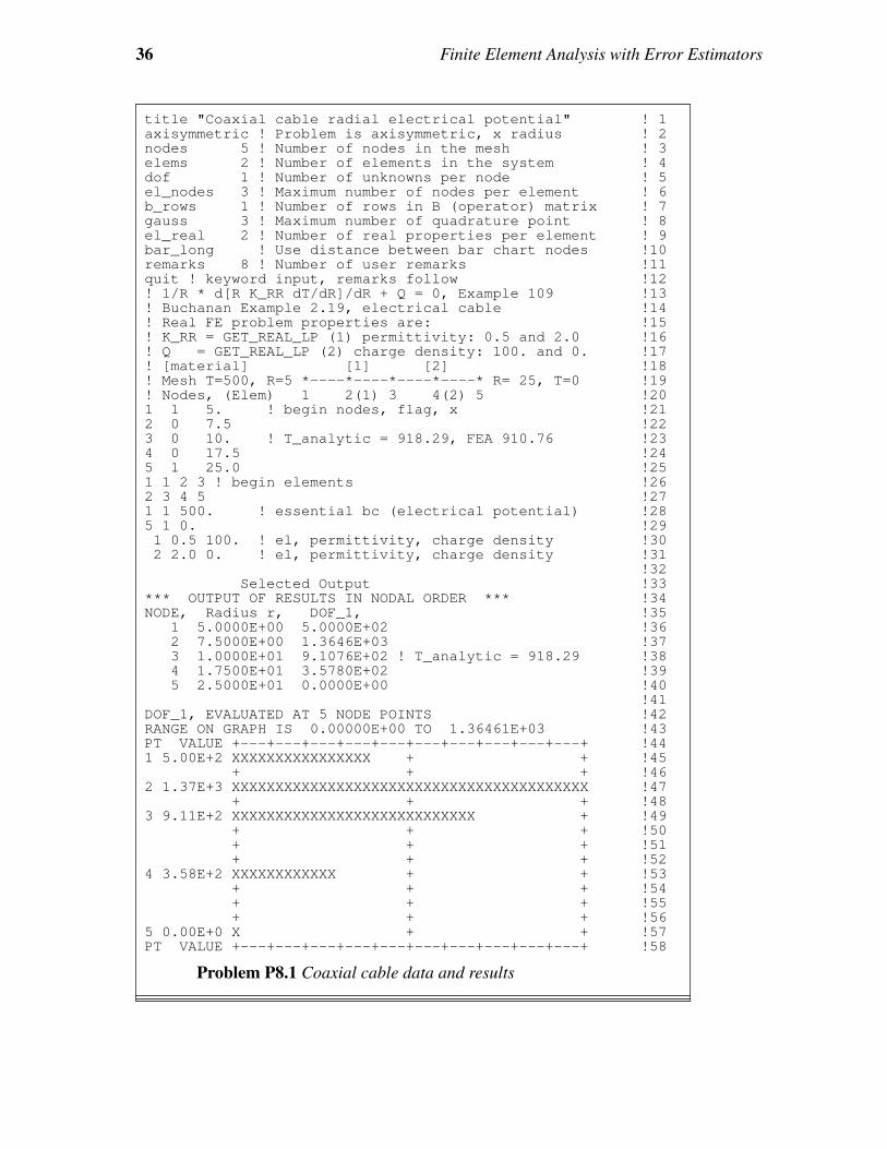
36 Finite Element Analysis with Error Estimators
title "Coaxial cable radial electrical potential" ! 1axisymmetric ! Problem is axisymmetric, x radius ! 2nodes 5 ! Number of nodes in the mesh ! 3elems 2 ! Number of elements in the system ! 4dof 1 ! Number of unknowns per node ! 5el_nodes 3 ! Maximum number of nodes per element ! 6b_rows 1 ! Number of rows in B (operator) matrix ! 7gauss 3 ! Maximum number of quadrature point ! 8el_real 2 ! Number of real properties per element ! 9bar_long ! Use distance between bar chart nodes !10remarks 8 ! Number of user remarks !11quit ! keyword input, remarks follow !12! 1/R * d[R K_RR dT/dR]/dR + Q = 0, Example 109 !13! Buchanan Example 2.19, electrical cable !14! Real FE problem properties are: !15! K_RR = GET_REAL_LP (1) permittivity: 0.5 and 2.0 !16! Q = GET_REAL_LP (2) charge density: 100. and 0. !17! [material] [1] [2] !18! Mesh T=500, R=5 *----*----*----*----* R= 25, T=0 !19! Nodes, (Elem) 1 2(1) 3 4(2) 5 !201 1 5. ! begin nodes, flag, x !212 0 7.5 !223 0 10. ! T_analytic = 918.29, FEA 910.76 !234 0 17.5 !245 1 25.0 !251 1 2 3 ! begin elements !262 3 4 5 !271 1 500. ! essential bc (electrical potential) !285 1 0. !291 0.5 100. ! el, permittivity, charge density !302 2.0 0. ! el, permittivity, charge density !31
!32Selected Output !33
*** OUTPUT OF RESULTS IN NODAL ORDER *** !34NODE, Radius r, DOF_1, !35
1 5.0000E+00 5.0000E+02 !362 7.5000E+00 1.3646E+03 !373 1.0000E+01 9.1076E+02 ! T_analytic = 918.29 !384 1.7500E+01 3.5780E+02 !395 2.5000E+01 0.0000E+00 !40
!41DOF_1, EVALUATED AT 5 NODE POINTS !42RANGE ON GRAPH IS 0.00000E+00 TO 1.36461E+03 !43PT VALUE +---+---+---+---+---+---+---+---+---+---+ !441 5.00E+2 XXXXXXXXXXXXXXXX + + !45
+ + + !462 1.37E+3 XXXXXXXXXXXXXXXXXXXXXXXXXXXXXXXXXXXXXXXXX !47
+ + + !483 9.11E+2 XXXXXXXXXXXXXXXXXXXXXXXXXXXX + !49
+ + + !50+ + + !51+ + + !52
4 3.58E+2 XXXXXXXXXXXX + + !53+ + + !54+ + + !55+ + + !56
5 0.00E+0 X + + !57PT VALUE +---+---+---+---+---+---+---+---+---+---+ !58
Problem P8.1 Coaxial cable data and results

Chapter 13, Solutions and Examples 37
1.9 Problems from chapter 9
Problem 9.1 Use the subroutines in Fig. 4.5.2 to form similar functions for a C1
rectangular element by taking a tensor product of the one-dimensional Hermite
interpolation relations. This will be a 16 degree of freedom element since each node will
have u, ∂u / ∂x, ∂u / ∂y, and ∂2u / ∂x∂y as nodal unknowns. Solution: Taking the
products of the 1-D functions yields the interpolations and first derivatives shown in
P9.1a and P9.1b. Such and element would usually be needed for a fourth order
differential equation which would have the second derivatives in the integral form. Thus
a similar subroutine for the second derivatives would be needed too.
Problem 9.5 Verify that if the above Q4 element maps onto a rectangle, with is sides
parallel to the global axes, of length L x and height L y then the Jacobian is constant at all
points in the element. Solution: Shown in Section 11.6.
SUBROUTINE SHAPE_16_R (R, S, A, B, H) ! 1! *-* *-* *-* *-* *-* *-* *-* *-* *-* *-* *-* ! 2! C1 RECTANGULAR ELEMENT IN UNIT COORDINATES ! 3! USING TENSOR PRODUCTS OF 1D HERMITE BASIS ! 4! *-* *-* *-* *-* *-* *-* *-* *-* *-* *-* *-* ! 5Use Precision_Module ! 6IMPLICIT NONE ! 7REAL(DP), INTENT(IN) :: R, S, A, B ! 8REAL(DP), INTENT(OUT) :: H (16) ! 9REAL(DP) :: HR (4), HS (4) !10
!11! DOF ARE W W,X W,Y W,XY AT EACH NODE (N_G_DOF=4) !12! X // R, Y // S. S !13! A = PHYSICAL LENGTH IN X 4 -------- 3 !14! B = PHYSICAL LENGTH IN Y I I !15! R,S = LOCAL UNIT COORDS I I !16! 1 at (0,0), 3 at (1,1) 1 -------- 2 ->R !17
!18! Evaluate the 1D Hermite interpolations !19CALL SHAPE_C1_L (R, A, HR) ; CALL SHAPE_C1_L (S, B, HS) !20
!21! Form tensor products !22
H (1) = HR (1) * HS (1) ; H (2) = HR (2) * HS (1) !23H (3) = HR (1) * HS (2) ; H (4) = HR (2) * HS (2) !24H (5) = HR (3) * HS (1) ; H (6) = HR (4) * HS (1) !25H (7) = HR (3) * HS (2) ; H (8) = HR (4) * HS (2) !26H (9) = HR (3) * HS (3) ; H (10) = HR (4) * HS (3) !27H (11) = HR (3) * HS (4) ; H (12) = HR (4) * HS (4) !28H (13) = HR (1) * HS (3) ; H (14) = HR (2) * HS (3) !29H (15) = HR (1) * HS (4) ; H (16) = HR (2) * HS (4) !30
END SUBROUTINE SHAPE_16_R !31
Problem P9.1a Shape functions from 1-D C1 products
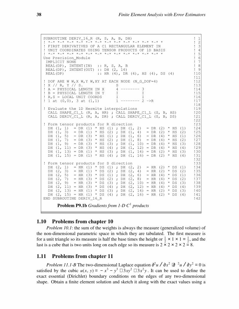
38 Finite Element Analysis with Error Estimators
SUBROUTINE DERIV_16_R (R, S, A, B, DH) ! 1! *-* *-* *-* *-* *-* *-* *-* *-* *-* *-* *-* *-* * ! 2! FIRST DERIVATIVES OF A C1 RECTANGULAR ELEMENT IN ! 3! UNIT COORDINATES USING TENSOR PRODUCTS OF 1D BASIS ! 4! *-* *-* *-* *-* *-* *-* *-* *-* *-* *-* *-* *-* * ! 5Use Precision_Module ! 6IMPLICIT NONE ! 7REAL(DP), INTENT(IN) :: R, S, A, B ! 8REAL(DP), INTENT(OUT) :: DH (2, 16) ! 9REAL(DP) :: HR (4), DR (4), HS (4), DS (4) !10
!11! DOF ARE W W,X W,Y W,XY AT EACH NODE (N_G_DOF=4) !12! X // R, Y // S. S !13! A = PHYSICAL LENGTH IN X 4 -------- 3 !14! B = PHYSICAL LENGTH IN Y I I !15! R,S = LOCAL UNIT COORDS I I !16! 1 at (0,0), 3 at (1,1) 1 -------- 2 ->R !17
!18! Evaluate the 1D Hermite interpolations !19
CALL SHAPE_C1_L (R, A, HR) ; CALL SHAPE_C1_L (S, B, HS) !20CALL DERIV_C1_L (R, A, DR) ; CALL DERIV_C1_L (S, B, DS) !21
!22! Form tensor products for R direction !23
DH (1, 1) = DR (1) * HS (1) ; DH (1, 2) = DR (2) * HS (1) !24DH (1, 3) = DR (1) * HS (2) ; DH (1, 4) = DR (2) * HS (2) !25DH (1, 5) = DR (3) * HS (1) ; DH (1, 6) = DR (4) * HS (1) !26DH (1, 7) = DR (3) * HS (2) ; DH (1, 8) = DR (4) * HS (2) !27DH (1, 9) = DR (3) * HS (3) ; DH (1, 10) = DR (4) * HS (3) !28DH (1, 11) = DR (3) * HS (4) ; DH (1, 12) = DR (4) * HS (4) !29DH (1, 13) = DR (1) * HS (3) ; DH (1, 14) = DR (2) * HS (3) !30DH (1, 15) = DR (1) * HS (4) ; DH (1, 16) = DR (2) * HS (4) !31
!32! Form tensor products for S direction !33
DH (2, 1) = HR (1) * DS (1) ; DH (2, 2) = HR (2) * DS (1) !34DH (2, 3) = HR (1) * DS (2) ; DH (2, 4) = HR (2) * DS (2) !35DH (2, 5) = HR (3) * DS (1) ; DH (2, 6) = HR (4) * DS (1) !36DH (2, 7) = HR (3) * DS (2) ; DH (2, 8) = HR (4) * DS (2) !37DH (2, 9) = HR (3) * DS (3) ; DH (2, 10) = HR (4) * DS (3) !38DH (2, 11) = HR (3) * DS (4) ; DH (2, 12) = HR (4) * DS (4) !39DH (2, 13) = HR (1) * DS (3) ; DH (2, 14) = HR (2) * DS (3) !40DH (2, 15) = HR (1) * DS (4) ; DH (2, 16) = HR (2) * DS (4) !41
END SUBROUTINE DERIV_16_R !42
Problem P9.1b Gradients from 1-D C1 products
1.10 Problems from chapter 10Problem 10.1: the sum of the weights is always the measure (generalized volume) of
the non-dimensional parametric space in which they are tabulated. The first measure is
for a unit triangle so its measure is half the base times the height or 1
2× 1 × 1 = 1
2, and the
last is a cube that is two units long on each edge so its measure is 2 × 2 × 2 × 2 = 8.
1.11 Problems from chapter 11
Problem 11.1-B The two-dimensional Laplace equation ∂2u / ∂x2 + ∂2u / ∂y2 = 0 is
satisfied by the cubic u(x, y) = − x3 − y3 + 3xy2 + 3x2 y . It can be used to define the
exact essential (Dirichlet) boundary conditions on the edges of any two-dimensional
shape. Obtain a finite element solution and sketch it along with the exact values using a

Chapter 13, Solutions and Examples 39
domain of: a) the above unit square, or b) a rectangle over 0 ≤ x ≤ 3 and 0 ≤ y ≤ 2, or c) a
quarter circle of radius 2 centered at the origin.
Clearly selecting a cubic element would give the exact solution everywhere, so we
want to use lower order elements to illustrate the error estimator. Here we show an
irregular mesh of 482 linear (T3) triangular elements and 273 nodes of which the 62 on
the boundary have had values assigned from the exact solution. That was done by
including the keyword controls of exact_case 20 and use_exact_bc to override the null
input values. We also turned on controls list_exact, list_exact_ flux so that the printed
output (omitted here) could be used to contrast the FEA results. Since we have giv en
formulations for both general numerically integrated elements and the T3 elements we
have to existing approaches that just need data. Here we have used the hard codes T3
form, selected with example 202. The mesh was obtained by starting with a crude mesh
and running two solutions through the error estimator to adapt to the input mesh shown in
P11.1Ba. The computed solution is given in P11.1Bb.
The FEA and exact solution contours along with their corresponding flux vectors
(using Fourier law signs) are comparable in P11.1Bc. Since the exact solution is known
we can compute the exact error in the solution at each node and contour them as in
P11.1Bd. Of course, the SCP error estimator uses the different energy norm values to
guide the adaptivity. Each element energy norm error estimate is constant. Next we
av erage the element energy norm error estimates at each node and contour that
distribution to compare it to the exact energy norm error estimates available from the
given analytic solution. These two sets of contours are compared in P11.1Be and their
agreement is quite good.
Problem 11.6 Solve the fin example of Fig. 11.5.14 by hand: a) with insulated edges, b)
with edge convection. Solution: The insulated edge case is given in detail in the text by
Allaire. The edge convection case requires three edge convection elements but will give
very similar results because the edges are so thin. In other words, one just assembles the
edge effects onto the previous algebraic equations. The new data are indicated in Fig.
P11.6Ba, the mesh and contours in P11.6Bb, and selected corresponding results are
shown in Fig. P11.6Bc. The net convection loss changes little.
Problem 11.8c For the conduction mesh in Figs.11.9 and 11 prepare a combined surface
plot of the element and SCP flux for: c) the RMS values.
Solution: Post processing each element gives the constant flux values of:
*** FLUX COMPONENTS AT ELEMENT INTEGRATION POINTS ***ELEMENT, PT, X-Coord, Y-Coord, FLUX_1, FLUX_2
1 1 1.3333E+00 6.6667E-01 -4.0000E+00 -2.5000E+002 1 3.3333E+00 6.6667E-01 -1.1000E+01 0.0000E+003 1 2.6667E+00 1.3333E+00 -8.5000E+00 -2.5000E+004 1 3.3333E+00 2.6667E+00 -8.5000E+00 0.0000E+00
Av eraging them via the patches gav e the values in Fig. 11.11. The RMS values of the
two results are combined in Problem P11.8.

40 Finite Element Analysis with Error Estimators
0 0.5 1 1.5 2 2.5 3
0
0.2
0.4
0.6
0.8
1
1.2
1.4
1.6
1.8
2
X for 482 Elements with 3 nodes
Y
FE Mesh; 273 Nodes, 62 with BC or MPC Noted
Problem P11.1Ba Mesh and Dirichlet condition points
00.5
11.5
22.5
3
0
0.5
1
1.5
2
−20
−10
0
10
20
30
40
50
X
FEA Solution Component_1: 482 Elements, 273 Nodes, (3 per Element)
Y
Com
pone
nt 1
(m
ax =
55,
min
= −
27)
Problem P11.1Bb Result carpet plot for linear triangles
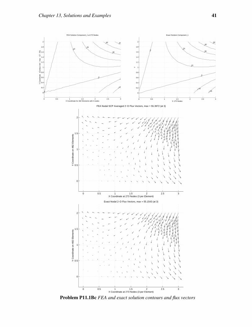
Chapter 13, Solutions and Examples 41
0 0.5 1 1.5 2 2.5 3
0
0.2
0.4
0.6
0.8
1
1.2
1.4
1.6
1.8
2
−20
−10
0
0
1020
30
40 50
FEA Solution Component_1 at 273 Nodes
X Coordinate for 482 Elements with 3 nodes
Y C
oord
inat
e (
Con
tour
min
: m
ax −
27 :
55)
0 0.5 1 1.5 2 2.5 3
0
0.2
0.4
0.6
0.8
1
1.2
1.4
1.6
1.8
2
−20
−10
0
0
10
20
30
4050
Exact Solution Component_1
X: 273 Nodes
Y
0 0.5 1 1.5 2 2.5 3
0
0.5
1
1.5
2
X Coordinate at 273 Nodes (3 per Element)
Y C
oord
inat
e on
482
Ele
men
ts
FEA Nodal SCP Averaged 2−D Flux Vectors, max = 55.3972 (at 3)
0 0.5 1 1.5 2 2.5 3
0
0.5
1
1.5
2
X Coordinate at 273 Nodes (3 per Element)
Y C
oord
inat
e on
482
Ele
men
ts
Exact Nodal 2−D Flux Vectors, max = 55.1543 (at 3)
Problem P11.1Bc FEA and exact solution contours and flux vectors

42 Finite Element Analysis with Error Estimators
0 0.5 1 1.5 2 2.5 3
0
0.2
0.4
0.6
0.8
1
1.2
1.4
1.6
1.8
2
0.02
0.020.02
0.02
0.02
0.04
0.04
0.06
0.06
X: 273 Nodes
YExact Error in Solution Component_1
Problem P11.1Bd Exact error at the mesh nodes
0 0.5 1 1.5 2 2.5 3
0
0.2
0.4
0.6
0.8
1
1.2
1.4
1.6
1.8
2
10
10
10
20
20
20
30
30
30
40
40
50
X: 482 Elements (with 3 nodes)
Y: 2
73 N
odes
FEA SCP Energy Norm Error Estimate Averaged at Nodes, % * 100
0 0.5 1 1.5 2 2.5 3
0
0.2
0.4
0.6
0.8
1
1.2
1.4
1.6
1.8
2
10
10
10
20
20
20
30
3030
40
40
40
50
X: 482 Elements (with 3 nodes)
Y: 2
73 N
odes
Exact Energy Norm Error Averaged at Nodes, % * 100
Problem P11.1Be SCP and exact averaged energy norm error
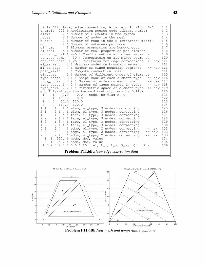
Chapter 13, Solutions and Examples 43
title "Fin face, edge convection, Allaire p343 2T3, 3L2" ! 1example 209 ! Application source code library number ! 2elems 2 ! Number of elements in the system ! 3nodes 4 ! Number of nodes in the mesh ! 4b_rows 2 ! Number of rows in the B (operator) matrix ! 5dof 1 ! Number of unknowns per node ! 6el_homo ! Element properties are homogeneous ! 7el_real 5 ! Number of real properties per element ! 8convect_coef 1.e-5 ! Coefficient on all mixed segments ! 9convect_temp 30 ! Temperature on all mixed segments !10convect_thick 1.25 ! Thickness for edge convections <= new !11el_segment 3 ! Maximum nodes on boundary segment !12mixed_segs 7 ! Number of mixed boundary segments <= new !13post_mixed ! Compute convection loss !14el_types 3 ! Number of different types of elements !15type_shape 2 2 1 ! Shape code of each element type <= new !16type_nodes 3 3 2 ! Number of nodes on each type <= new !17type_gauss 1 4 2 ! Number of Gauss points in types <= new !18type_parm 2 2 1 ! Parametric space of element type <= new !19end ! Terminate the keyword control, remarks follow !201 1 0.0 0.0 ! node, bc-flag,x, y !213 1 160.0 0.0 !222 0 50.0 120.0 !234 0 110.0 120.0 !241 1 1 3 4 ! elem, el_type, 3 nodes. conducting !252 1 2 1 4 ! elem, el_type, 3 nodes. conducting !261 2 1 3 4 ! face, el_type, 3 nodes. convecting !272 2 2 1 4 ! face, el_type, 3 nodes. convecting !283 2 1 3 4 ! face, el_type, 3 nodes. convecting !294 2 2 1 4 ! face, el_type, 3 nodes. convecting !305 3 3 4 ! edge, el_type, 2 nodes. convecting <= new !316 3 4 2 ! edge, el_type, 2 nodes. convecting <= new !327 3 2 1 ! edge, el_type, 2 nodes. convecting <= new !33
1 1 330. ! node, dof, value !343 1 250. ! node, dof, value !35
1 0.2 0.2 0.0 0.0 1.25 ! el, k_x, k_y, K_xy, Q, thick !36
Problem P11.6Ba New edge convection data
0 20 40 60 80 100 120 140 160
0
20
40
60
80
100
120
X: 9 Elements
Y: 4
Nod
es
FE Mesh Geometry: 3 Types, 9 Elements, 4 Nodes
1
2
3
4
1
2
3
4
5
6
7
8
9
Fin with edge convection
0 20 40 60 80 100 120 140 160
0
20
40
60
80
100
120 180200
220240
260
280
300
320
Matlab Smoothed FEA Component_1 (176.756 to 330)
X: 9 Elements with 3 nodes
Y o
n 9
Ele
men
ts
Fin with edge convection
Problem P11.6Bb New mesh and temperature contours
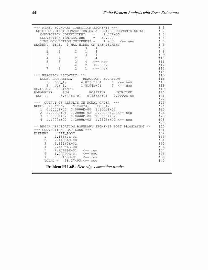
44 Finite Element Analysis with Error Estimators
*** MIXED BOUNDARY CONDITION SEGMENTS *** ! 1NOTE: CONSTANT CONVECTION ON ALL MIXED SEGMENTS USING ! 2
CONVECTION COEFFICIENT = 1.00E-05 ! 3CONVECTION TEMPERATURE = 30.000 ! 4LINE CONVECTION THICKNESS = 1.250 <== new ! 5
SEGMENT, TYPE, 3 MAX NODES ON THE SEGMENT ! 61 2 1 3 4 ! 72 2 2 1 4 ! 83 2 1 3 4 ! 94 2 2 1 4 !105 3 3 4 <== new !116 3 4 2 <== new !127 3 2 1 <== new !13
!14*** REACTION RECOVERY *** !15
NODE, PARAMETER, REACTION, EQUATION !161, DOF_1, 4.0271E+01 1 <== new !173, DOF_1, 1.8104E+01 3 <== new !18
REACTION RESULTANTS !19PARAMETER, SUM POSITIVE NEGATIVE !20DOF_1, 5.8375E+01 5.8375E+01 0.0000E+00 !21
!22*** OUTPUT OF RESULTS IN NODAL ORDER *** !23NODE, X-Coord, Y-Coord, DOF_1, !24
1 0.0000E+00 0.0000E+00 3.3000E+02 !252 5.0000E+01 1.2000E+02 2.0404E+02 <== new !263 1.6000E+02 0.0000E+00 2.5000E+02 !274 1.1000E+02 1.2000E+02 1.7676E+02 <== new !28
!29** BEGIN APPLICATION BOUNDARY SEGMENTS POST PROCESSING ** !30*** CONVECTION HEAT LOSS *** !31ELEMENT HEAT_LOST !32
1 2.13362E+01 !332 7.44956E+00 !343 2.13362E+01 !354 7.44956E+00 !365 2.97989E-01 <== new !376 1.20299E-01 <== new !387 3.85158E-01 <== new !39TOTAL = 58.37493 <== new !40
Problem P11.6Bc New edge convection results

Chapter 13, Solutions and Examples 45
0
1
2
3
4
0
1
2
3
4
5
6
7
8
9
10
11
12
13
14
Y
FEA T3 and SCP Flux RMS Value: 4 Elements, 6 Nodes, (3 per Element)
X
RM
S F
lux
Val
ue
Problem P11.8c Constant and SCP RMS flux surfaces
Problem 11.7 For the solid conducting bar of Fig. 11.2.2 assume a length L = 8 cm, a
width 2W = 4 cm, and a thickness of 2H = 1 cm. The material has a thermal
conductivity of k = 3 W /cm C, is surrounded by a fluid at a temperature of Θ∞ = 20 C,
and has a surface convection coefficient of h = 0. 1 W /cm2 C. Employ two equal length
conduction elements and associated face, line, or point convection elements to obtain a
solution for the temperature distribution and the convection heat loss. Use conduction
elements that are: a) linear line elements, b) bilinear rectangular elements, c) trilinear
brick elements.
Solution: We hav e developed most of the necessary linear element matrices to formulate
a hand solution and could produce the few missing forms easily since the Jacobian matrix
for the conduction elements has a constant diagonal form. Instead we will use the
numerically integrated general routines in Fig. 11.8.1, for all conduction effects, Fig.
11.8.3 to form the convection matrices, and finally Fig. 11.8.4 to post-process the
convection elements to determine the convection heat loss, by recovering the integral of
Hb evaluated in Fig. 11.8.3. These routines could be used with any of the linear,
quadratic, or cubic elements in the current library.
1.12 Problems from chapter 12
Problem 12.1 Implement the isotropic Ee matrix for the plane strain assumption
with the stress components in the xx, yy, xy order. Solution: the listing in Problem P12.1.
Problem 12.2 Implement the isotropic Ee matrix for the general solid with the stress
components in the xx, yy, xy, zz, xz, yz order. Solution: see listing Problem P12.2.

46 Finite Element Analysis with Error Estimators
SUBROUTINE E_PLANE_STRAIN (E) ! 1! * * * * * * * * * * * * * * * * * * * * * * * * * * * * * ! 2! PLANE_STRAIN CONSTITUTIVE MATRIX DEFINITION ! 3! STRESS & STRAIN COMPONENT ORDER: XX, YY, XY, SO N_R_B = 3 ! 4! PROPERTY ORDER: 1-YOUNG’S MODULUS, 2-POISSON’S RATIO ! 5! * * * * * * * * * * * * * * * * * * * * * * * * * * * * * ! 6Use System_Constants ! for DP, N_R_B ! 7Use Sys_Properties_Data ! for function GET_REAL_LP ! 8IMPLICIT NONE ! 9REAL(DP), INTENT(OUT) :: E (N_R_B, N_R_B) ! Constitutive !10REAL(DP) :: C_1, C_2, P_R, S_M, Y_M ! Miscellaneous !11
!12! N_R_B = NUMBER OF ROWS IN B AND E MATRICES !13! P_R = POISSON’S RATIO, S_M = SHEAR MODULUS !14! Y_M = YOUNG’S MODULUS OF ELASTICITY !15
!16IF ( EL_REAL < 2 ) STOP ’KEYWORD el_real<2 IN E_PLANE_STRAIN’ !17Y_M = GET_REAL_LP (1) ; P_R = GET_REAL_LP (2) !18
!19C_1 = Y_M * (1 - P_R) / ((1 + P_R)*(1 - P_R - P_R)) !20C_2 = Y_M * P_R / ((1 + P_R)*(1 - P_R - P_R)) !21S_M = 0.5d0 * Y_M / ( 1 + P_R) !22E (1, 1) = C_1 ; E (2, 1) = C_2 ; E (3, 1) = 0.d0 !23E (1, 2) = C_2 ; E (2, 2) = C_1 ; E (3, 2) = 0.d0 !24E (1, 3) = 0.d0 ; E (2, 3) = 0.d0 ; E (3, 3) = S_M !25
END SUBROUTINE E_PLANE_STRAIN !26
Problem P12.1 Plane strain assumption isotropic constitutive law
SUBROUTINE E_SOLID_STRESS (E) ! 1! * * * * * * * * * * * * * * * * * * * * * * * * * * * * * ! 2! SOLID_STRESS CONSTITUTIVE MATRIX DEFINITION ! 3! STRESS COMPONENT ORDER: XX, YY, XY, ZZ, XZ, YZ, SO N_R_B = 6 ! 4! PROPERTY ORDER: 1-YOUNG’S MODULUS, 2-POISSON’S RATIO ! 5! * * * * * * * * * * * * * * * * * * * * * * * * * * * * * ! 6Use System_Constants ! for DP, N_R_B ! 7Use Sys_Properties_Data ! for function GET_REAL_LP ! 8IMPLICIT NONE ! 9REAL(DP), INTENT(OUT) :: E (N_R_B, N_R_B) ! Constitutive !10REAL(DP) :: C_1, C_2, P_R, S_M, Y_M ! Miscellaneous !11
!12! N_R_B = NUMBER OF ROWS IN B AND E MATRICES !13! P_R = POISSON’S RATIO, S_M = SHEAR MODULUS !14! Y_M = YOUNG’S MODULUS OF ELASTICITY !15
!16IF ( N_R_B /= 6 ) STOP ’INVALID N_R_B IN E_SOLID_STRESS’ !17IF (EL_REAL < 2) STOP ’KEY el_real < 2 IN E_SOLID_STRESS’ !18Y_M = GET_REAL_LP (1) ; P_R = GET_REAL_LP (2) !19
!20C_1 = Y_M * (1 - P_R) / (1 + P_R) / (1 - P_R - P_R) !21C_2 = C_1 * P_R / (1 - P_R); S_M = 0.5d0 * Y_M / (1 + P_R) !22E = 0.d0 ! Mostly !23E (1, 1) = C_1 ; E (2, 1) = C_2 ; E (4, 1) = C_2 ! normals !24E (1, 2) = C_2 ; E (2, 2) = C_1 ; E (4, 2) = C_2 ! normals !25E (1, 4) = C_2 ; E (2, 4) = C_2 ; E (4, 4) = C_1 ! normals !26E (3, 3) = S_M ; E (5, 5) = S_M ; E (6, 6) = S_M ! shears !27
END SUBROUTINE E_SOLID_STRESS !28
Problem P12.2 Isotropic solid constitutive matrix

Chapter 13, Solutions and Examples 47
SUBROUTINE ELASTIC_B_SOLID (DGH, B) ! 1! * * * * * * * * * * * * * * * * * * * * * * * * * * * * ! 2! 3-D ELASTICITY STRAIN-DISPLACEMENT RELATIONS (B) ! 3! * * * * * * * * * * * * * * * * * * * * * * * * * * * * ! 4Use System_Constants ! for DP, N_R_B, N_G_DOF, N_SPACE ! 5Use Elem_Type_Data ! for LT_FREE, LT_N ! 6IMPLICIT NONE ! 7REAL(DP), INTENT(IN) :: DGH (N_SPACE, LT_N) ! 8REAL(DP), INTENT(OUT) :: B (N_R_B, LT_N * N_G_DOF) ! 9INTEGER :: J, K, L, M !10
!11! B = STRAIN-DISPLACEMENT MATRIX (RETURNED) !12! DGH = GLOBAL DERIVATIVES OF ELEM INTERPOLATIONS !13! LT_N = NUMBER OF NODES PER ELEMENT !14! N_G_DOF = NUMBER OF PARAMETERS PER NODE !15! N_R_B = NUMBER OF STRAINS (IN B) XX, YY, XY, ZZ, XZ, YZ !16! N_SPACE = DIMENSION OF SPACE !17
!18B = 0.d0 !19DO J = 1, LT_N ! ROW NUMBER !20
K = N_G_DOF * (J - 1) + 1 ! FIRST COLUMN, U TERMS !21L = K + 1 ! SECOND COLUMN, V TERMS !22M = L + 1 ! THIRD COLUMN, W TERMS !23B (1, K) = DGH (1, J) ! DU/DX FOR XX NORMAL !24B (3, K) = DGH (2, J) ! DU/DY FOR XY SHEAR !25B (5, K) = DGH (3, J) ! DU/DZ FOR XZ SHEAR !26B (2, L) = DGH (2, J) ! DV/DY FOR YY NORMAL !27B (3, L) = DGH (1, J) ! DV/DX FOR XY SHEAR !28B (6, L) = DGH (3, J) ! DV/DZ FOR YZ SHEAR !29B (4, M) = DGH (3, J) ! DW/DZ FOR ZZ NORMAL !30B (5, M) = DGH (1, J) ! DW/DX FOR XZ SHEAR !31B (6, M) = DGH (2, J) ! DW/DY FOR YZ SHEAR !32
END DO !33END SUBROUTINE ELASTIC_B_SOLID !34
Problem P12.3 Strain-displacement matrix for a general solid

48 Finite Element Analysis with Error Estimators
! .............................................................. ! 1! *** ELEM_SQ_MATRIX PROBLEM DEPENDENT STATEMENTS FOLLOW *** ! 2! .............................................................. ! 3! Note: BODY (N_SPACE) is available through the interface ! 4! Linear Triangle, T3, Plane stress only ! 5! STRESS AND STRAIN COMPONENT ORDER: XX, YY, XY, SO N_R_B = 3 ! 6REAL(DP):: X_I, X_J, X_K, Y_I, Y_J, Y_K ! Global coordinates ! 7REAL(DP):: A_I, A_J, A_K, B_I, B_J, B_K ! Standard geometry ! 8REAL(DP):: C_I, C_J, C_K, X_CG, Y_CG, TWO_A ! Standard geometry ! 9REAL(DP):: THICK ! Element thickness !10
!11! DEFINE NODAL COORDINATES, CCW: I, J, K !12
X_I = COORD (1,1) ; X_J = COORD (2,1) ; X_K = COORD (3,1) !13Y_I = COORD (1,2) ; Y_J = COORD (2,2) ; Y_K = COORD (3,2) !14
!15! DEFINE CENTROID COORDINATES (QUADRATURE POINT) !16
X_CG = (X_I + X_J + X_K)/3.d0 ; Y_CG = (Y_I + Y_J + Y_K)/3.d0 !17!18
! GEOMETRIC PARAMETERS H_I (X,Y) = (A_I + B_I*X + C_I*Y)/TWO_A !19A_I = X_J * Y_K - X_K * Y_J; B_I = Y_J - Y_K; C_I = X_K - X_J !20A_J = X_K * Y_I - X_I * Y_K; B_J = Y_K - Y_I; C_J = X_I - X_K !21A_K = X_I * Y_J - X_J * Y_I; B_K = Y_I - Y_J; C_K = X_J - X_I !22
!23! CALCULATE TWICE ELEMENT AREA !24
TWO_A = A_I + A_J + A_K ! = B_J*C_K - B_K*C_J also !25!26
! DEFINE 3 BY 6 STRAIN-DISPLACEMENT MATRIX, B !27B (1, 1:6) = (/ B_I, 0.d0, B_J, 0.d0, B_K, 0.d0 /)/TWO_A !28B (2, 1:6) = (/ 0.d0, C_I, 0.d0, C_J, 0.d0, C_K /)/TWO_A !29B (3, 1:6) = (/ C_I, B_I, C_J, B_J, C_K, B_K /)/TWO_A !30
!31CALL E_PLANE_STRESS (E) ! THE CONSTITUTIVE MATRIX !32THICK = 1 ; IF ( AREA_THICK /= 1.d0 ) THICK = AREA_THICK !33TWO_A = TWO_A * THICK ! true volume !34
!35! STIFFNESS MATRIX, WITH CONSTANT JACOBIAN !36
S = MATMUL ( TRANSPOSE (B), MATMUL (E, B) ) * TWO_A * 0.5d0 !37!38
! BODY FORCE PER UNIT VOLUME !39IF ( HAS_BODY_FORCE ) THEN ! values in Body_Force array !40
C (1:5:2) = BODY_FORCE (1) * TWO_A / 6.d0 ! X component !41C (2:6:2) = BODY_FORCE (2) * TWO_A / 6.d0 ! Y component !42
END IF ! or set up properties for body force !43!44
! SAVE ONE POINT RULE TO AVERAGING, OR ERROR ESTIMATOR !45LT_QP = 1 ; CALL STORE_FLUX_POINT_COUNT ! Save LT_QP !46CALL STORE_FLUX_POINT_DATA ( (/ X_CG, Y_CG /), E, B ) !47
!48if ( DEBUG_EL_SQ ) then !49
print *,’S matrix:’ ; call rprint (S, LT_FREE, LT_FREE, 1) !50print *,’C matrix:’ ; call rprint (C, 1, LT_FREE, 1) !51
end if !52! End of application dependent code !53! *** END ELEM_SQ_MATRIX PROBLEM DEPENDENT STATEMENTS *** !54
Problem P12.4 Stiffness for isotropic plane stress CST

Chapter 13, Solutions and Examples 49
SUBROUTINE ELASTICITY_E_MATRIX (E) ! 1! * * * * * * * * * * * * * * * * * * * * * * * * * * * * * ! 2! ELASTICITY CONSTITUTIVE MATRIX DEFINITION ! 3! * * * * * * * * * * * * * * * * * * * * * * * * * * * * * ! 4Use System_Constants ! for DP, N_R_B, N_SPACE, ! 5
! AXISYMMETRIC, PLANE_STRAIN ! 6IMPLICIT NONE ! 7REAL(DP), INTENT(OUT) :: E (N_R_B, N_R_B) ! CONSTITUTIVE ! 8
! N_R_B = NUMBER OF ROWS IN B AND E MATRICES ! 9! E = SYMMETRIC CONSTITUTIVE MATRIX !10
!11IF ( ANISOTROPIC ) THEN !12
STOP ’ELASTICITY_E_MATRIX: ANISOTROPIC E UNAVAILABLE’ !13! SELECT CASE (N_SPACE) !14! CASE (1) ! 1-D or cylinder !15! IF ( AXISYMMETRIC ) THEN ! Components RR & TT !16! CALL ANISOTROPIC_CYL_STRESS (E) !17! ELSE ! Component XX !18! CALL E_BAR_STRESS (E) ; END IF !19! CASE (2) ! 2-D or axisymmetric !20! IF ( AXISYMMETRIC ) THEN ! Components RR ZZ RZ TT !21! CALL ANISOTROPIC_AXI_STRESS (E) !22! ELSE IF ( PLANE_STRAIN ) THEN ! Components XX YY XY !23! CALL ANISOTROPIC_2D_STRAIN (E) !24! ELSE ! plane stress Components XX YY XY !25! CALL ANISOTROPIC_2D_STRESS (E) ; END IF !26! CASE (3) ! 3-D !27! CALL ANISOTROPIC_3D_STRESS (E) ! XX YY XY ZZ ZX ZY !28! END SELECT !29ELSE ! Isotropic !30
!31SELECT CASE (N_SPACE) !32
!33CASE (1) ! 1-D or cylinder !34
IF ( AXISYMMETRIC ) THEN ! Components RR & TT !35! CALL E_CYLINDER_STRESS (E) !36ELSE ! Component XX !37! CALL E_BAR_STRESS (E) !38END IF !39
!40CASE (2) ! 2-D or axisymmetric !41
IF ( AXISYMMETRIC ) THEN ! Components RR ZZ RZ TT !42CALL E_AXISYMMETRIC_STRESS (E) !43
ELSE IF ( PLANE_STRAIN ) THEN ! Components XX YY XY !44CALL E_PLANE_STRAIN (E) !45
ELSE ! plane stress Components XX YY XY !46CALL E_PLANE_STRESS (E) ; END IF !47
!38CASE (3) ! 3-D !49
CALL E_SOLID_STRESS (E) ! XX YY XY ZZ ZX ZY !50!51
END SELECT !52END IF ! anisotropic material !53END SUBROUTINE ELASTICITY_E_MATRIX !54
Problem P12.5 A general elasticity constitutive matrix control
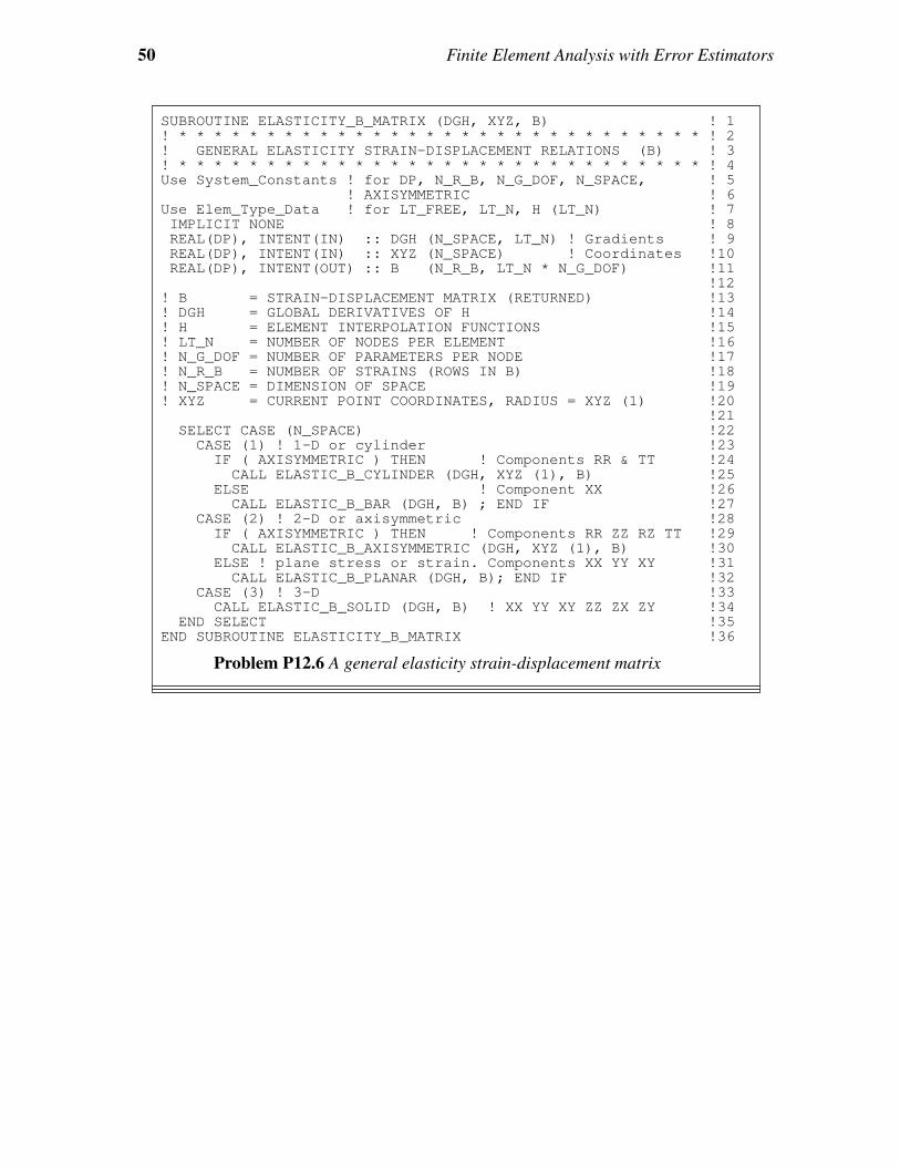
50 Finite Element Analysis with Error Estimators
SUBROUTINE ELASTICITY_B_MATRIX (DGH, XYZ, B) ! 1! * * * * * * * * * * * * * * * * * * * * * * * * * * * * * * ! 2! GENERAL ELASTICITY STRAIN-DISPLACEMENT RELATIONS (B) ! 3! * * * * * * * * * * * * * * * * * * * * * * * * * * * * * * ! 4Use System_Constants ! for DP, N_R_B, N_G_DOF, N_SPACE, ! 5
! AXISYMMETRIC ! 6Use Elem_Type_Data ! for LT_FREE, LT_N, H (LT_N) ! 7IMPLICIT NONE ! 8REAL(DP), INTENT(IN) :: DGH (N_SPACE, LT_N) ! Gradients ! 9REAL(DP), INTENT(IN) :: XYZ (N_SPACE) ! Coordinates !10REAL(DP), INTENT(OUT) :: B (N_R_B, LT_N * N_G_DOF) !11
!12! B = STRAIN-DISPLACEMENT MATRIX (RETURNED) !13! DGH = GLOBAL DERIVATIVES OF H !14! H = ELEMENT INTERPOLATION FUNCTIONS !15! LT_N = NUMBER OF NODES PER ELEMENT !16! N_G_DOF = NUMBER OF PARAMETERS PER NODE !17! N_R_B = NUMBER OF STRAINS (ROWS IN B) !18! N_SPACE = DIMENSION OF SPACE !19! XYZ = CURRENT POINT COORDINATES, RADIUS = XYZ (1) !20
!21SELECT CASE (N_SPACE) !22
CASE (1) ! 1-D or cylinder !23IF ( AXISYMMETRIC ) THEN ! Components RR & TT !24
CALL ELASTIC_B_CYLINDER (DGH, XYZ (1), B) !25ELSE ! Component XX !26
CALL ELASTIC_B_BAR (DGH, B) ; END IF !27CASE (2) ! 2-D or axisymmetric !28
IF ( AXISYMMETRIC ) THEN ! Components RR ZZ RZ TT !29CALL ELASTIC_B_AXISYMMETRIC (DGH, XYZ (1), B) !30
ELSE ! plane stress or strain. Components XX YY XY !31CALL ELASTIC_B_PLANAR (DGH, B); END IF !32
CASE (3) ! 3-D !33CALL ELASTIC_B_SOLID (DGH, B) ! XX YY XY ZZ ZX ZY !34
END SELECT !35END SUBROUTINE ELASTICITY_B_MATRIX !36
Problem P12.6 A general elasticity strain-displacement matrix

Chapter 13, Solutions and Examples 51
! *** ELEM_SQ_MATRIX PROBLEM DEPENDENT STATEMENTS *** ! 1! STATIC PLANE_STRAIN ANALYSIS, NON-ISOPARAMETRIC ! 2! with BODY_FORCE (N_SPACE) via keyword control and/or ! 3! DYNAMIC with mass matrix EL_M (LT_FREE, LT_FREE) ! 4! ------------------------------------------------------------ ! 5! STRESS AND STRAIN COMPONENT ORDER: XX, YY, XY, SO N_R_B = 3 ! 6! LATER PLUS ZZ & EFFECTIVE AS N_R_B + 1 & 2 ! 7
! 8INTEGER :: IP ! loops ! 9REAL(DP) :: DET, DET_WT ! volume !10REAL(DP) :: N_e (N_G_DOF, LT_FREE) ! interpolation !11REAL(DP), SAVE :: RHO=1.d0 ! data !12
!13! N_G_DOF = NUMBER OF GENERALIZED PARAMETERS (DOF) PER NODE !14! N_e = GENERALIZED INTERPOLATION ARRAY !15! PROPERTIES: 1-YOUNG’S MODULUS, 2-POISSON’S RATIO, AND !16! 3-YIELD STRESS, IF PRESENT, 4-MASS DENSITY, IF PRESENT !17
!18IF ( EL_REAL > 3 ) RHO = GET_REAL_LP (4) ! Mass density !19N_e = 0.d0 ! Save zeros !20CALL STORE_FLUX_POINT_COUNT ! Save LT_QP !21
!22! FORM THE CONSTITUTIVE MATRIX (OR GET_APPLICATION_E_MATRIX) !23CALL E_PLANE_STRAIN (E) !24
!25DO IP = 1, LT_QP ! NUMERICAL INTEGRATION LOOP !26
G = GET_G_AT_QP (IP) ! GEOMETRY INTERPOLATIONS !27GEOMETRY = COORD (1:LT_GEOM,:) ! GEOMETRY NODES !28XYZ = MATMUL (G, GEOMETRY) ! COORDINATES OF POINT !29
!30DLG = GET_DLG_AT_QP (IP) ! GEOMETRIC DERIVATIVES !31AJ = GEOMETRIC_JACOBIAN () ! JACOBIAN !32CALL INVERT_2BY2 (AJ, AJ_INV, DET) ! INVERSE, DET !33DET_WT = DET * WT (IP) !34
!35H = GET_H_AT_QP (IP) ! SCALAR INTERPOLATIONS !36N_e (1, 1:LT_FREE:2) = H ! Fill vector interpolations !37N_e (2, 2:LT_FREE:2) = H ! Fill vector interpolations !38DLH = GET_DLH_AT_QP (IP) ! SCALAR DERIVATIVES !39DGH = MATMUL (AJ_INV, DLH) ! PHYSICAL DERIVATIVES !40
!41!---> FORM STRAIN DISPLACEMENT, B (OR GET_APPLICATION_B_MATRIX) !42
CALL ELASTIC_B_PLANAR (DGH, B) !43!44
! EVALUATE ELEMENT STIFFNESS, MASS MATRICES !45S = S + DET_WT * MATMUL (TRANSPOSE(B), MATMUL (E, B)) !46EL_M = EL_M + MATMUL (TRANSPOSE(N_e), N_e) * DET_WT * RHO !47
!48! EVALUATE ANY BODY FORCE RESULTANTS !49
IF ( HAS_BODY_FORCE ) THEN !50C = C + MATMUL (TRANSPOSE(N_e), BODY_FORCE(1:2)) * DET_WT !51
END IF !52!53
! SAVE PT, CONSTITUTIVE & STRAIN_DISP FOR POST_PROCESS & SCP !54CALL STORE_FLUX_POINT_DATA (XYZ, E, B) !55
END DO ! Over quadrature points !56! *** END ELEM_SQ_MATRIX PROBLEM DEPENDENT STATEMENTS *** !57
Problem P12.7a Plane strain analysis with body force and mass matrix
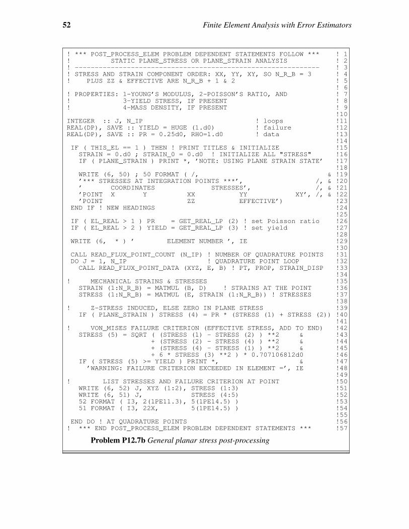
52 Finite Element Analysis with Error Estimators
! *** POST_PROCESS_ELEM PROBLEM DEPENDENT STATEMENTS FOLLOW *** ! 1! STATIC PLANE_STRESS OR PLANE_STRAIN ANALYSIS ! 2! ------------------------------------------------------------- ! 3! STRESS AND STRAIN COMPONENT ORDER: XX, YY, XY, SO N_R_B = 3 ! 4! PLUS ZZ & EFFECTIVE ARE N_R_B + 1 & 2 ! 5
! 6! PROPERTIES: 1-YOUNG’S MODULUS, 2-POISSON’S RATIO, AND ! 7! 3-YIELD STRESS, IF PRESENT ! 8! 4-MASS DENSITY, IF PRESENT ! 9
!10INTEGER :: J, N_IP ! loops !11REAL(DP), SAVE :: YIELD = HUGE (1.d0) ! failure !12REAL(DP), SAVE :: PR = 0.25d0, RHO=1.d0 ! data !13
!14IF ( THIS_EL == 1 ) THEN ! PRINT TITLES & INITIALIZE !15
STRAIN = 0.d0 ; STRAIN_0 = 0.d0 ! INITIALIZE ALL "STRESS" !16IF ( PLANE_STRAIN ) PRINT *, ’NOTE: USING PLANE STRAIN STATE’ !17
!18WRITE (6, 50) ; 50 FORMAT ( /, & !19’*** STRESSES AT INTEGRATION POINTS ***’, /, & !20’ COORDINATES STRESSES’, /, & !21’POINT X Y XX YY XY’, /, & !22’POINT ZZ EFFECTIVE’) !23
END IF ! NEW HEADINGS !24!25
IF ( EL_REAL > 1 ) PR = GET_REAL_LP (2) ! set Poisson ratio !26IF ( EL_REAL > 2 ) YIELD = GET_REAL_LP (3) ! set yield !27
!28WRITE (6, * ) ’ ELEMENT NUMBER ’, IE !29
!30CALL READ_FLUX_POINT_COUNT (N_IP) ! NUMBER OF QUADRATURE POINTS !31DO J = 1, N_IP ! QUADRATURE POINT LOOP !32
CALL READ_FLUX_POINT_DATA (XYZ, E, B) ! PT, PROP, STRAIN_DISP !33!34
! MECHANICAL STRAINS & STRESSES !35STRAIN (1:N_R_B) = MATMUL (B, D) ! STRAINS AT THE POINT !36STRESS (1:N_R_B) = MATMUL (E, STRAIN (1:N_R_B)) ! STRESSES !37
!38! Z-STRESS INDUCED, ELSE ZERO IN PLANE STRESS !39
IF ( PLANE_STRAIN ) STRESS (4) = PR * (STRESS (1) + STRESS (2)) !40!41
! VON_MISES FAILURE CRITERION (EFFECTIVE STRESS, ADD TO END) !42STRESS (5) = SQRT ( (STRESS (1) - STRESS (2) ) **2 & !43
+ (STRESS (2) - STRESS (4) ) **2 & !44+ (STRESS (4) - STRESS (1) ) **2 & !45+ 6 * STRESS (3) **2 ) * 0.707106812d0 !46
IF ( STRESS (5) >= YIELD ) PRINT *, & !47’WARNING: FAILURE CRITERION EXCEEDED IN ELEMENT =’, IE !48
!49! LIST STRESSES AND FAILURE CRITERION AT POINT !50
WRITE (6, 52) J, XYZ (1:2), STRESS (1:3) !51WRITE (6, 51) J, STRESS (4:5) !5252 FORMAT ( I3, 2(1PE11.3), 5(1PE14.5) ) !5351 FORMAT ( I3, 22X, 5(1PE14.5) ) !54
!55END DO ! AT QUADRATURE POINTS !56
! *** END POST_PROCESS_ELEM PROBLEM DEPENDENT STATEMENTS *** !57
Problem P12.7b General planar stress post-processing

Chapter 13, Solutions and Examples 53
Problem 12.3 Give an implementation of the Be matrix for a general solid. Assume the
strain components are in the xx, yy, xy, zz, xz, yz order. Solution: listing Problem P12.3.
Problem 12.4 Review the scalar implementation for the T3 element, given in Fig. 10.4.1,
and extend it to the case of a two-dimensional stress model. Solution: an explicit hard
code version of this element is given in Problem P12.4.
Problem 12.5 Implement a general evaluation of the elasticity Ee matrix that will handle
all the 1-, 2-, and 3-dimensional cases. Solution: see listing Problem P12.5.
Problem 12.6 Implement a general evaluation of the elasticity Be matrix that will handle
all the 1-, 2-, and 3-dimensional cases. Solution: see listing Problem P12.6.
Problem 12.7 Modify the plane stress implementation shown in Figs. 12.4.5 and 6 to
solve a plane strain problem. Remember that an additional normal stress must be
considered in the post-processing stage. Validate the results with a patch test. Solution:
The square matrix formulation is shown in P.12.7a which has been generalized to include
the element mass matrix, EL_M , for possible use in a dynamic solution. If only static
problems are of interest then line 47 should be omitted. Also of interest are lines 37 and
38 where the scalar interpolation array He has been inserted into the non-zero terms of
the generalized interpolation array N via an implied loop in each row. The mass matrix is
twice as big as in the scalar cases of Chapter 11 because we must account for mass
distribution in both directions. Also note that Ne is used in computing the body force
resultant vector in line 51. The necessary input, if globally constant, can be supplied by a
control keyword body_ force followed by a value for each spatial dimension. That also
makes the logical variable HAS_BODY _FORCE true.
The post-processing is slightly generalized in P12.7b. It defaults to a plane stress
post-processing (σ z = 0) unless the keyword plane_strain appears in the control data.
Line 40 shows the σ z recovery if it is not zero. Likewise, the effective stress of line 43 is
valid for either planar result. Since we had to recover two extra stresses at this stage the
system allocates (n_r_b + 2) storage locations for the stress and strain arrays since one
often wants to keep actual failure results with the stress or strain on which they are based.
However, this sometimes requires the specification of range sizes, as in lines 36 and 37
that would not be necessary if recovered items were stored in separate arrays. The
element formulation is valid for any element in the library, and the results and post-
processing were validated using a patch test.