seismic detection of cold production footprints - crewes · seismic detection of cold production...

Seismic detection of cold production footprints

CREWES Research Report — Volume 15 (2003) 1

Cold production footprints of heavy oil on time-lapse seismology: Lloydminster field, Alberta

Sandy Chen, Laurence R. Lines, Joan Embleton, P.F. Daley, and Larry Mayo*

ABSTRACT The simultaneous extraction of oil and sand during the cold production of heavy oil

generates high permeability channels termed as “wormholes”. The development of wormholes causes reservoir pressure decrease below the bubble point, resulting in dissolved gas out of solution to form foamy oil. The foamy oil could fill depressurized drainage regions (production footprints) around the borehole, leading to fluid phase changes. In this paper, the upper bound and lower bound models on the fluid mixture bulk moduli have been used to detect the sensitivity of seismic P-wave velocity. Then the Gassmann Equation has been employed to calculate the bulk modulus variations of the drainage rocks, where the velocity and density decrease dramatically due to some exolved gas. A 2D cold production model has been built to examine the seismic responses of drainage regions based on well logs in the Lloydminster cold production pool. The seismic modelling responses indicate amplitude anomalies and traveltime delays in these regions upon comparison of pre and post production results. However, because most heavy oil cold production reservoirs are very thin, with less than 10 m of net pay, seismic resolution is a challenge. Different seismic frequency bandwidths have also been tested to look at how vertical seismic resolution determines the detection of the drainage regions.

INTRODUCTION The extraction of heavy oil by cold production is a non-thermal process, in which sand

and oil are produced simultaneously to enhance the oil recovery. This process has been economically successful in several unconsolidated heavy oilfields in Alberta and Saskatchewan. The reason for this is that producing sand creates a wormhole network and a foamy oil drive. These two effects are key to boosting oil recovery.

Wormhole networks During the cold production process, both heavy oil and sand are transported to the

surface using a progressive cavity pump, generating sharp pressure gradients in the reservoir. This results in a failure of the unconsolidated sand matrix. The failed sand flows to the well, triggering the development of wormholes. Sawatzky and Lillico (2002) believe that wormholes grow in unconsolidated, clean sand layers within the net pay zone, along the highest pressure gradient between the borehole and the tip of the wormhole. Wormholes usually can grow to a distance of 150 m or more from the original boreholes, forming approximately horizontal high permeability channels in the reservoirs. Based on the laboratory experiments conducted by the Alberta Research Council (ARC), Tremblay et al. (1999) observed that the porosity of the mature wormholes could reach

* EnCana Corporation

Chen et al.

2 CREWES Research Report — Volume 15 (2003)

50% or more. He also determined wormhole diameters could range from the order of 10 cm to 1 metre as the maximum size. Wormholes play an important role in the improvement of the reservoir permeability. However, Sawatzky believes that the wormhole density cannot exceed 5% of the total net pay. In this case, the wormhole contribution to the average porosity of the net pay is relatively small.

Foamy oil drives The cold production process involves the depressurization of the reservoir while

wormholes grow. The pressure falls below the bubble point, resulting in the exsolution of dissolved gases as bubbles within the oil. The viscosity and specific gravity of heavy oil restrict the gas bubbles from coalescing into a separate phase. Thus, the trapped gas bubbles within the heavy oil form the foamy oil (Figure 1a). The formation of foamy oil increases the fluid volume within the reservoir, generating the high pressure, forcing grains apart and driving both oil and gas to the wells through the wormholes (Figure 1b). Therefore, the foamy oil drive within the reservoir enhances oil recovery.

(a) (b)

FIG. 1. a) Foamy oil (Greenidge, ESSO); b) Single propagating wormhole in sand reservoirs (Dusseault, 1994), where foamy oil drives the oil and gas to the low pressure wormhole.

Drainage footprints The drainage footprints could be considered as regions that are depressurized. In cold

production, the extent of the drainage region is strongly related to the growth of wormholes, where reservoir pressure has decreased. The drainage region can expand at least as far as the length of wormholes through the entire net pay. Sawatzky and Lillico (2002) showed a likely drainage footprint scenario for the cold production wells in the small Southwest Saskatchewan heavy oil pool (Figure 2), which helped engineers design infill drills and development plan. Engineers also believe that 3D time-lapse seismology could be a tool implemented in the imaging of the drainage region, caused by foamy oil and the presence of wormholes. Mayo (1996) showed some amplitude anomalies caused by foamy oil effects in a 3D time-lapse seismic survey from cold production in the Lloydminster area (Figure 3). The 3D survey was required 9 years after production began. Mayo believes that the amplitude anomalies around the boreholes could represent the drainage regions.



FIG. 2. Most likely depletion (drainage) footprint scenario for the cold production wells in the small southwest Saskatchewan heavy oil pool.(Sawatzky, 2002).

FIG. 3. Seismic amplitude extraction from the MacLaren horizon (Mayo, 1999). The 3D seismic survey shot 9 years after the pool was discovered shows amplitude anomalies.

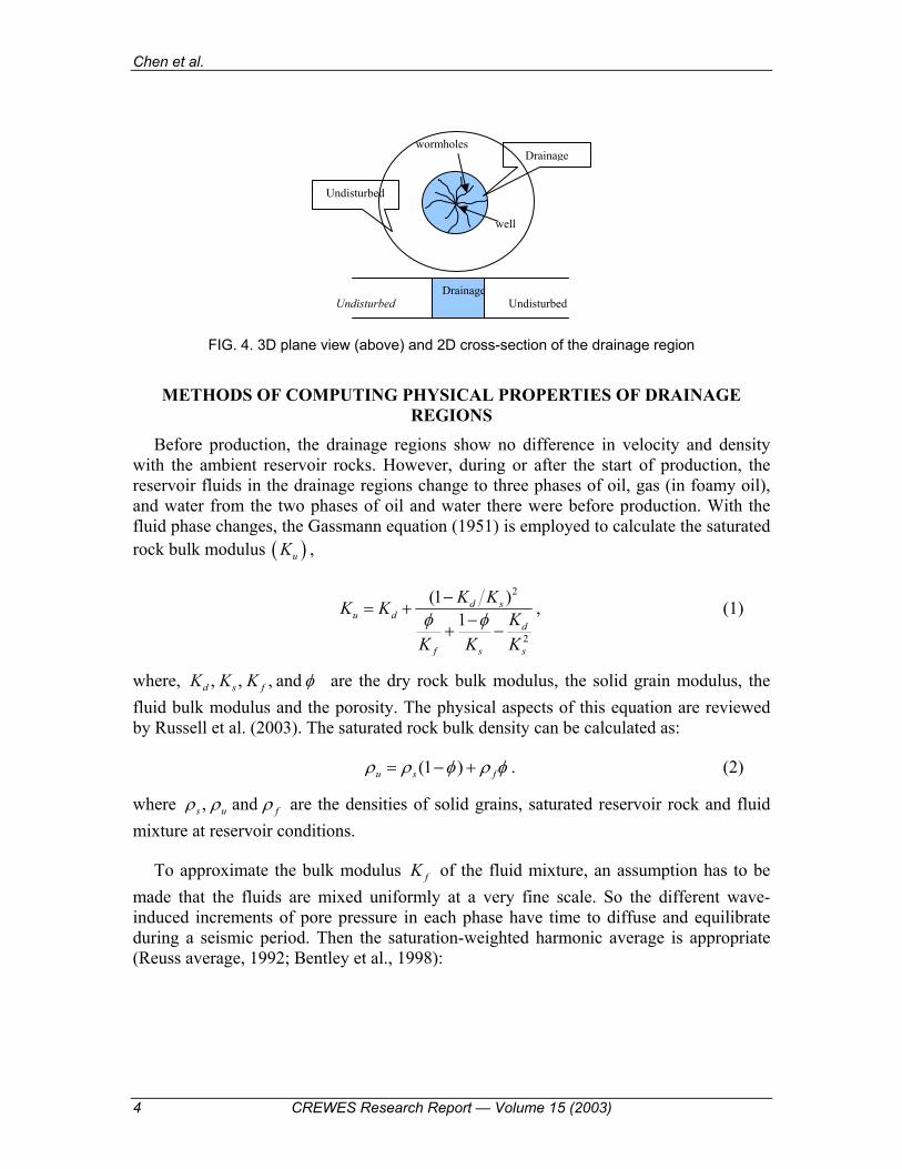
Based on the characteristics of the heavy oil cold-production footprints, we built a simplified 3D model as a cylinder around the borehole, representing the drainage region of heavy oil cold production (Figure 4), which shows a 3D plane view and a 2D cross-section of the drainage region. Before production, most of the heavy oil cold-production reservoirs are highly saturated with oil, and a small partial of water. After the start of the production, with sand extraction and wormhole growth, the fluid phases change into oil, water, and foamy oil with gas bubbles. Therefore, the drainage regions are highly disturbed with the presence of foamy oil, and can be significantly different from the initial reservoir state of oil and water only.

From what we saw in Figure 3, the question was raised of whether or not the foamy oil effects can explain seismic amplitude anomalies. This is the key study of this paper.

Chen et al.


FIG. 4. 3D plane view (above) and 2D cross-section of the drainage region

METHODS OF COMPUTING PHYSICAL PROPERTIES OF DRAINAGE REGIONS

Before production, the drainage regions show no difference in velocity and density with the ambient reservoir rocks. However, during or after the start of production, the reservoir fluids in the drainage regions change to three phases of oil, gas (in foamy oil), and water from the two phases of oil and water there were before production. With the fluid phase changes, the Gassmann equation (1951) is employed to calculate the saturated rock bulk modulus ( )uK ,

2

2

(1 )1

d su d

d

f s s

K KK K KK K Kφ φ

−= +

−+ −

, (1)

where, , , , andd s fK K K φ are the dry rock bulk modulus, the solid grain modulus, the fluid bulk modulus and the porosity. The physical aspects of this equation are reviewed by Russell et al. (2003). The saturated rock bulk density can be calculated as:

(1 )u s fρ ρ φ ρ φ= − + . (2)

where , ands u fρ ρ ρ are the densities of solid grains, saturated reservoir rock and fluid mixture at reservoir conditions.

To approximate the bulk modulus fK of the fluid mixture, an assumption has to be made that the fluids are mixed uniformly at a very fine scale. So the different wave-induced increments of pore pressure in each phase have time to diffuse and equilibrate during a seismic period. Then the saturation-weighted harmonic average is appropriate (Reuss average, 1992; Bentley et al., 1998):

Drainage

Undisturbed

wormholes

well

Undisturbed Undisturbed Drainage



1 g o w

f g o w

S S SK K K K

= + + , (3)

Where, , andg o wS S S are the gas, oil and water saturations, respectively. In this situation, any small amount of gas will cause the estimate of the fluid mixture bulk modulus to be very low. In order to compute the bulk moduli of gas ( )gK , oil ( )oK and water ( )wK , the methods demonstrated by Batzle and Wang (1992) are applied. The fluid mixture density is a volume average given by:

f g g o o w wS S Sρ ρ ρ ρ= + + . (4)

In order to estimate the dry bulk modulus, we have to use the two equations:

u

up

KVρµ 3/4+

= , (5)

u

sVρµ

= (6)

Here µ is the shear modulus of saturated rock. As PV is known from the sonic log (Figure 5) and the P SV V ratio of 1.9 derived from one of the dipole sonic logs in Pikes Peak area, we can obtain the values of uK and µ based on equations. (5) and (6). Applying them to equation (1), the dry rock bulk modulus can be derived. In this case, we assume that the dry bulk modulus of rocks remains constant before and after production although slight differences of porosities exist between the drainage region and the undisturbed region.

Finally, the Gassmann Equation can be employed to calculate the saturated rock bulk modulus Ku and shear modulus under in-situ reservoir conditions after production. Table 1 shows the in-situ reservoir parameters before and after a 3-year production period provided by Sawatzky (ARC). Table 2 contains the physical properties of reservoir rock in the drainage regions before and after production calculated using the above formula. With a 10% gas saturation, the saturated rock bulk modulus dramatically drops from 10.6 Gpa to 5.2 Gpa, while the shear bulk modulus shows only a slight increase. Hence the P-wave velocity has decreased from 2795 m/s to 2325 m/s, and the S-wave velocity has increased slightly due to the density decrease.

Chen et al.


The sensitivity of seismic velocities to pore fluids depends not only on saturations but also on the spatial distributions of the phase within the rock (Mavko et al., 1998). Therefore, another assumption is made that the fluids are “patchy” at a scale that is smaller than the seismic wavelength, but larger than the scale at which the scale fluids can equilibrate pressures through local flow. The effective fluid bulk modulus is then larger, which defines the upper bound on the fluid mixture bulk modulus. The upper bound of the fluid mixture bulk modulus is an isotrain average, known as the Voigt model:

K S K S K S Kg g o o w wf = + + . (7)

Table 1. In-situ reservoir parameters in drainage regions

Production: Pre Post Vp (m/s) from logs 2795 unknown Vp/Vs (from logs) 1.9 unknown density from log (g/cm3) 2.16 unknown density of grain sand (g/cm3) 2.65 2.65 oil API 11.3 11.3 specific gravity of methane 0.56 0.56 gas pseudocritical temperature (F) -116.5 -116.5 gas pseudocritical pressure (Psi) 667 667 solution Gas-Oil ratio 7.5 7.5 reservoir temperature (C) 20 20 reservoir pressure (kPa) 3000 1500 water saturation (%) 20 20 oil saturation (%) 80 70 gas saturation (%) 0 10 water salinity (ppm) 44000 44000 porosity (%) 30 30

Table 2. Physical properties of drainage region before and after production using lower bound on fluid bulk modulus

Before production After production Sg=0, So=0.8 Sg=0.1, So=0.7 saturated rock bulk modulus (Gpa) 10.616 5.2252 saturated shear modulus (Gpa) 4.6726 4.6777 saturated bulk density (kg/m3) 2156.5 2126.6 Vp (m/s) 2795 2325 Vs (m/s) 1472 1483



Table 3 shows the variations of bulk moduli and seismic velocities when applying the equation (7), where the saturated rock bulk modulus and P-wave velocity are only slightly different from that in Table 2.

So, equation (3) actually defines the lower bound of the fluid mixture bulk modulus. And any other distribution of fluid phases gives the moduli falling between these two bounds (Mavko et al., 1998).

Table 3. Physical properties of drainage region before and after production using upper bound on fluid bulk modulus

Before production After production Sg=0, So=0.8 Sg=0.1, So=0.7

saturated rock bulk modulus (Gpa) 10.616 10.113 saturated shear modulus (Gpa) 4.6726 4.6777 saturated bulk density (kg/m3) 2156.5 2126.6

Vp (m/s) 2795 2773 Vs (m/s) 1472 1483

Considering the uncertainty of the fluid state, the average fluid bulk moduli from equations (3) and (7) is applied to the Gassmann Equation. Then the average P-wave velocity and density (Table 4) will be employed to the following seismic modelling.

Table 4. Physical parameters of in-situ drainage region using the average of upper bound and lower bound on fluid bulk modulus

Saturated rock Preproduction Postproduction Sg=0, So=0.8 Sg=0.1, So=0.7

bulk modulus (Gpa) 10.616 7.807 shear modulus (Gpa) 4.671 4.676 bulk density (kg/m3) 2156 2126

Vp (m/s) 2795 2570 Vs (m/s) 1472 1483

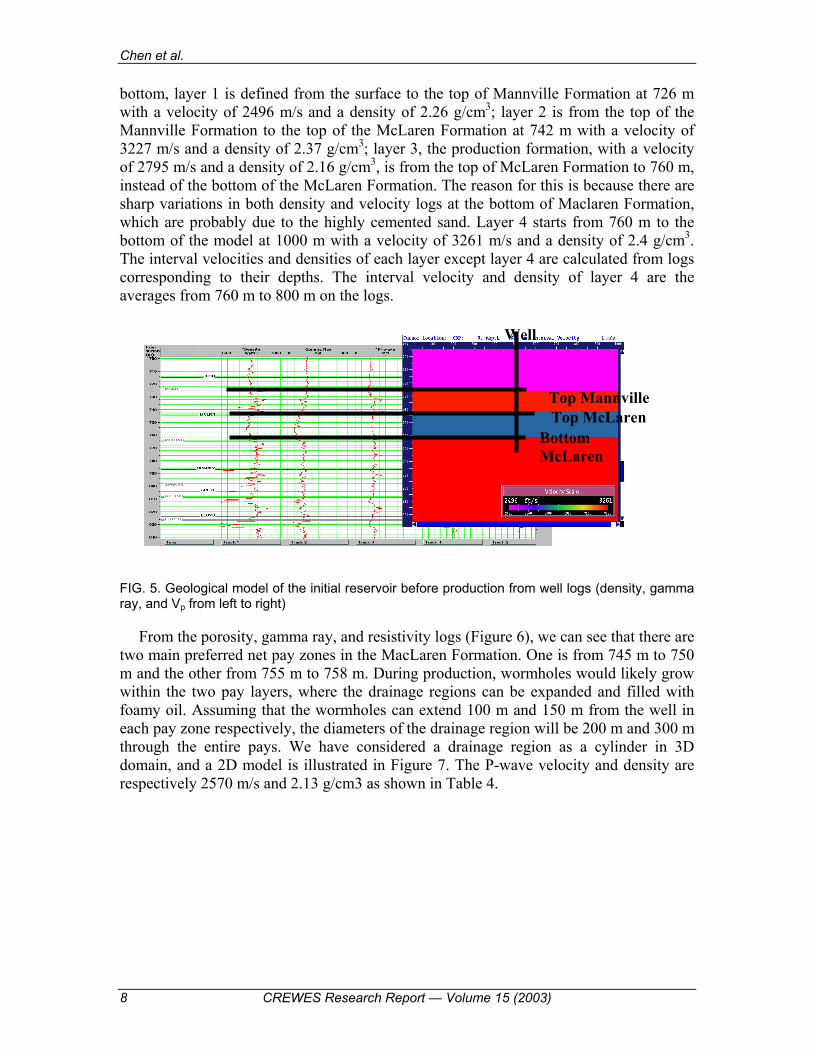
GEOLOGICAL MODELS Before production, the geological model was built based on the logs from one well

drilled by EnCana Corporation in the Lloydminster heavy oil cold production pool. The production zone is the McLaren Formation consisting of unconsolidated sandstones in the Upper Mannville BB Pool. According to the density, gamma ray, and P-wave velocity (converted from sonic) logs, a geological model of the initial reservoir has been built as shown in Figure 5. This model is 1000 m by 1000 m in the horizontal and vertical directions, consisting of four layers matched the variations of well logs. From top to

Chen et al.


bottom, layer 1 is defined from the surface to the top of Mannville Formation at 726 m with a velocity of 2496 m/s and a density of 2.26 g/cm3; layer 2 is from the top of the Mannville Formation to the top of the McLaren Formation at 742 m with a velocity of 3227 m/s and a density of 2.37 g/cm3; layer 3, the production formation, with a velocity of 2795 m/s and a density of 2.16 g/cm3, is from the top of McLaren Formation to 760 m, instead of the bottom of the McLaren Formation. The reason for this is because there are sharp variations in both density and velocity logs at the bottom of Maclaren Formation, which are probably due to the highly cemented sand. Layer 4 starts from 760 m to the bottom of the model at 1000 m with a velocity of 3261 m/s and a density of 2.4 g/cm3. The interval velocities and densities of each layer except layer 4 are calculated from logs corresponding to their depths. The interval velocity and density of layer 4 are the averages from 760 m to 800 m on the logs.

FIG. 5. Geological model of the initial reservoir before production from well logs (density, gamma ray, and Vp from left to right)

From the porosity, gamma ray, and resistivity logs (Figure 6), we can see that there are two main preferred net pay zones in the MacLaren Formation. One is from 745 m to 750 m and the other from 755 m to 758 m. During production, wormholes would likely grow within the two pay layers, where the drainage regions can be expanded and filled with foamy oil. Assuming that the wormholes can extend 100 m and 150 m from the well in each pay zone respectively, the diameters of the drainage region will be 200 m and 300 m through the entire pays. We have considered a drainage region as a cylinder in 3D domain, and a 2D model is illustrated in Figure 7. The P-wave velocity and density are respectively 2570 m/s and 2.13 g/cm3 as shown in Table 4.

Top McLaren Bottom McLaren

Top Mannville

Well



FIG. 6. Two main net pays (745-750 m, 755-758 m) in MacLaren reservoir sand, the upper one with 5 m net pay, and the lower one with 3 m

FIG. 7. The drainage region model after production within two net pays (upper one 5 m thick with a diameter of 200 m; the lower 3 m thick, a diameter of 300 m (in purple). Both have a velocity of 2570 m/s, a density of 2.13 g/cm3

MODELLING RESULTS

Based on the models shown in Figure 5 and 7, zero-offset seismic traces with and without drainage regions were generated using the exploding reflector, then a Kirchhoff depth migration was applied in the Promax software package.

The velocity and density grid is 1 m by 1 m. CDP intervals are 1 metre. Figure 8 illustrates the migrated sections of pre- and post-production, as well as the difference between the two at a frequency bandwidth of 200 Hz. We can observe the amplitude anomalies and traveltime delays caused by the two drainage regions, with lower velocity and density compared to the ambient rocks.

In order to detect seismic resolution effects on thin-bed drainage regions, we changed the frequency bandwidth from 200 Hz to 100 Hz and 50 Hz. Figure 8 illustrates that only

Well

Chen et al.


the cumulative responses of the two drainage regions can be observed due to lower resolutions. And it is almost unidentifiable in the 50 Hz case (shown in Figure 9). Compared to Figure 8, where the two drainage regions are clearly separated, we believe that the seismic frequency bandwidth plays an important role in imaging the drainage regions.

(a) Without the drainage regions (b) With the drainage regions

(c) Difference between (a) and (b)

FIG. 8. Time-lapse migrated sections with a frequency bandwidth of 200 Hz.

(a) With a frequency bandwidth of 100 Hz (b) With a frequency bandwidth of 50 Hz

FIG. 9. Migrated sections with the drainage regions.

CONCLUSIONS The cold production process in heavy oil is a unique procedure of producing oil and

sand simultaneously, while generating high-permeability wormhole channels within the



reservoir. The presence of wormholes with depleted pressures leads to significant changes in reservoir characteristics from the initial state of the reservoir. This makes seismic detection of drainage regions (production footprints) practical using time-lapse seismology techniques.

The length of the wormholes determines the extent of the drainage regions, also called production footprints. With the growth of wormholes, the reservoir pressures drop below the bubble point, the dissolved gas comes out of solution from the live oil, forming foamy oil. Hence, the exolved gas changes the fluid phases in the drainage regions, leading to P-wave velocity and density decreases. These physical properties cause “bright spots” on the synthetic seismic traces.

Since most net pays in cold production are less than 10 m thick, vertical seismic resolution is key on detecting the images of drainage regions, which are determined by the velocity and the frequency bandwidth.

ACKNOWLEDGEMENTS The authors thank the COURSE project and CREWES for their financial and technical

support. We acknowledge the contributions to our research made by Alberta Research Council. We also would like to thank Dr. Ron Sawatzky for his valuable suggestions and discussions.

REFERENCES Batzle, M. and Wang,Z., 1992, Seismic properties of pore fluids: Geophysics, 57, No. 11, P1396-1408. Bentley, L. and Zhang, J., 1999, Four-D seismic monitoring feasibility: CREWES Research Report, 11. Dusseault, M. 1994, Mechanisms and management of sand production: C-FER Project 88-06, Vol. 4. Gassmann, F., 1951, Elastic waves through a packing of spheres: Geophysics, 16, 637-685. Mayo, L., 1996, Seismic monitoring of foamy heavy oil, Lloydminster, Western Canada: 66th Ann.

Internat. Mtg. Soc. Of Expl. Geophys, 2091-2094. Russell, B.H., Hedlin, K., Hilterman, F., and Lines, L.R., 2003, Fluid-property discrimination with AVO: A

Boit-Gassmann perspective: Geophysics, 68, 29-39 Sawatzky, R.P. and Lillico, D.A., 2002, Tracking cold production footprints: CIPC Conference, Calgary,

Alberta, June11-13. Tremblay, B., 1999, A review of cold production in heavy oil reservoirs: EAGE 10th European Symposium

on Improved Oil Recovery, Brighton, UK.

seismic detection of cold production footprints - crewes · seismic detection of cold production...

Documents