seismic data processing with the parallel windowed ... · pdf fileseismic data processing with...

Seismic Data Processing with theParallel Windowed Curvelet

Transformby

Fadhel Alhashim

B.Sc. Software Engineering, King Fahad University of Petroleum and Minerals,Dhahran, 2004

A THESIS SUBMITTED IN PARTIAL FULFILMENT OFTHE REQUIREMENTS FOR THE DEGREE OF

Master of Science

in

The Faculty of Graduate Studies

(Geophysics)

THE UNIVERSITY OF BRITISH COLUMBIA

August, 2009

c© Fadhel Alhashim 2009

Abstract

The process of obtaining high quality seismic images is very challengingwhen exploring new areas that have high complexities. The to be processedseismic data comes from the field noisy and commonly incomplete. Recently,major advances were accomplished in the area of coherent noise removal, forexample, Surface Related Multiple Elimination (SRME).(Verschuur et al.,1992).

Predictive multiple elimination methods, such as SRME, consist of twosteps: The first step is the prediction step, in this step multiples are pre-dicted from the seismic data. The second step is the separation step inwhich primary reflection and surface related multiples are separated, thisinvolves predicted multiples from the first step to be ”matched” with thetrue multiples in the data and eventually removed (Verschuur, 2006; Wanget al., 2008). Wang et al.,2008 have introduced a robust Bayesian wavefieldseparation method to improve on the separation by matching methods. Thismethod utilizes the effectiveness of using the multi scale and multi angularcurvelet transform (Candes et al., 2006; Ying et al., 2005) in processing seis-mic images. The method produced excellent results and improved multipleremoval. A considerable problem in the seismic processing field is the factthat seismic data are large and require a correspondingly large memory sizeand processing time. The fact that curvelets are redundant also increasesthe need for large memory to process seismic data.

In this thesis we propose a parallel aproach based windowing operatorthat divides large seismic data into smaller more managable datasets thatcan fit in memory so that it is possible to apply the Bayesian separation pro-cess in parallel with minimal harm to the image quality and data integrity.However, by dividing the data, we introduce discontinuities. We take thesediscontinuities into account and compare two ways that different windowsmay communicate. The first method is to communicate edge informationat only two steps, namely, data scattering and gathering processes whileapplying the multiple separation on each window separately. The secondmethod is to define our windowing operator as a global operator, which

ii

Abstract

exchanges window edge information at each forward and inverse curvelettransform. We discuss the trade off between the two methods trying tominimize complexity and I/O time spent in the process.

We test our windowing operator on a seismic denoising problem andthen apply the windowing operator on our sparse-domain Bayesian primary-multiple seperation.

iii

Bibliography

Candes, E. J., L. Demanet, D. L. Donoho, and L. Ying, 2006, Fast discretecurvelet transforms: Multiscale Modeling and Simulation, 5, no. 3, 861–899.

Verschuur, D. J., 2006, Seismic multiple removal techniques: past, presentand future: EAGE publications b.v. ed.

Verschuur, D. J., A. J. Berkhout, and C. P. A. Wapenaar, 1992, Adaptivesurface-related multiple elimination: Geophysics, 57.

Wang, D., R. Saab, O. Yilmaz, and F. J. Herrmann, 2008, Bayesian-signalseparation by sparsity promotion: application to primary-multiple sepa-ration: Technical Report TR-2008-1, UBC Earth and Ocean Sciences De-partment.

Ying, L., L. Demanet, and E. J. Candes, 2005, 3-D discrete curvelet trans-form: Proceedings SPIE wavelets XI, San Diego, 5914, 344–354.

iv

Table of Contents

Abstract . . . . . . . . . . . . . . . . . . . . . . . . . . . . . . . . . ii

Bibliography . . . . . . . . . . . . . . . . . . . . . . . . . . . . . . . iv

Table of Contents . . . . . . . . . . . . . . . . . . . . . . . . . . . . v

List of Tables . . . . . . . . . . . . . . . . . . . . . . . . . . . . . . vii

List of Figures . . . . . . . . . . . . . . . . . . . . . . . . . . . . . . ix

Preface . . . . . . . . . . . . . . . . . . . . . . . . . . . . . . . . . . xii

Acknowledgments . . . . . . . . . . . . . . . . . . . . . . . . . . . xiii

Dedication . . . . . . . . . . . . . . . . . . . . . . . . . . . . . . . . xiv

1 Introduction . . . . . . . . . . . . . . . . . . . . . . . . . . . . . 11.1 Theme . . . . . . . . . . . . . . . . . . . . . . . . . . . . . . 31.2 Objectives . . . . . . . . . . . . . . . . . . . . . . . . . . . . 31.3 Outline . . . . . . . . . . . . . . . . . . . . . . . . . . . . . . 41.4 Theoretical background . . . . . . . . . . . . . . . . . . . . . 5

Bibliography . . . . . . . . . . . . . . . . . . . . . . . . . . . . . . . 9

2 Curvelet based seismic data processing . . . . . . . . . . . . 102.1 Curvelet based denoising . . . . . . . . . . . . . . . . . . . . 102.2 Curvelet based primary-multiple separation . . . . . . . . . . 10

2.2.1 Introduction . . . . . . . . . . . . . . . . . . . . . . . 102.2.2 Bayesian primary-multiple separation by sparsity pro-

motion . . . . . . . . . . . . . . . . . . . . . . . . . . 11

Bibliography . . . . . . . . . . . . . . . . . . . . . . . . . . . . . . . 18

v

Table of Contents

3 Parallel windowed seismic data processing . . . . . . . . . . 203.1 Parallel windowed curvelet transform . . . . . . . . . . . . . 203.2 Parallel windowed curvelet transform usage . . . . . . . . . . 243.3 Scalability . . . . . . . . . . . . . . . . . . . . . . . . . . . . 27

Bibliography . . . . . . . . . . . . . . . . . . . . . . . . . . . . . . . 31

4 Parallel seismic data processing with the parallel windowedcurvelet transform. . . . . . . . . . . . . . . . . . . . . . . . . . 324.1 Parallel windowed seismic data denoising . . . . . . . . . . . 324.2 Parallel windowed primary-multiple separation . . . . . . . . 33

4.2.1 2D data experiments . . . . . . . . . . . . . . . . . . 354.2.2 3D data experiments . . . . . . . . . . . . . . . . . . 38

Bibliography . . . . . . . . . . . . . . . . . . . . . . . . . . . . . . . 48

5 Conclusion . . . . . . . . . . . . . . . . . . . . . . . . . . . . . . 495.1 Parallel curvelet domain seismic data processing . . . . . . . 495.2 Open and future research . . . . . . . . . . . . . . . . . . . . 50

Bibliography . . . . . . . . . . . . . . . . . . . . . . . . . . . . . . . 51

vi

List of Tables

1.1 Advantages and disadvantages of Scenario A: windowing dataand applying separation seperatly, Scenario B: windowingdata with overlapping operators. . . . . . . . . . . . . . . . . 4

2.1 The iterative Bayesian wavefield separation algorithm intro-duced in Wang et al., 2008; Saab, 2008 . . . . . . . . . . . . . 13

2.2 Calculated SNR of estimated primaries using the Bayesianseparation. SNR was calculated against the ground truth“multiple-free” primaries. . . . . . . . . . . . . . . . . . . . . 14

4.1 Calculated SNR for the denoise problem. The first columnspecifies which scenario was used. Scenario A: no edge in-formation update during separation. Scenario B: edge infor-mation update occurs at each transform call. each pair ofrows share the same parameters used in scenario A and B.The window column shows the number of windows at eachdimension, these windows have identical sizes. . . . . . . . . . 34

4.2 Calculated SNR for the 2D synthetic data set. The first col-umn specifies which scenario was used. Scenario A: no edgeinformation update during separation. Scenario B: edge in-formation update occurs at each transform call. each pair ofrows share the same parameters used in scenario A and B.The difference column carry the difference between the SNRsof scenario A and B for each pair. The window column showsthe number of windows at each dimension, these windowshave identical sizes. Notice that the more windows we havethe more discontinuities in the data which lowers the SNR.Also, notice that increasing the overlap amount improves theSNR. All results were achieved after 10 iterations of the solver. 37

vii

List of Tables

4.3 Calculated SNR for the 3D synthetic data set. The first col-umn specifies which scenario was used. Scenario A: no edgeinformation update during separation. Scenario B: edge in-formation update occurs at each transform call. each pair ofrows share the same parameters used in scenario A and B.The difference column carry the difference between the SNRsof scenario A and B for each pair. The window column showsthe number of windows at each dimension, these windowshave identical sizes. Notice that the more windows we havethe more discontinuities in the data which lowers the SNR. . 38

viii

List of Figures

1.1 Synthetic data consisting of three primaries and six surfacerelated multiples. Top: the waves paths. Bottom: seismicdata of the waves above. Notice that primaries reflect oncewhile multiples reflect more than once resulting in some falsehorizons or reflectors on the seismic image. Adapted fromIkelle and Amundsen, 2005 . . . . . . . . . . . . . . . . . . . 2

1.2 Four curvelets with the same angle but different scales start-ing from coarsest scale to finest scale left to right in the a)spatial domain b) Fourier or frequency domain . . . . . . . . 7

1.3 Principle of alignment. Curvelets and wavefronts that locallyhave the same frequency content and direction produce largeinner products (significant coefficients). Adapted from Her-rmann and Hennenfent, 2008. . . . . . . . . . . . . . . . . . . 7

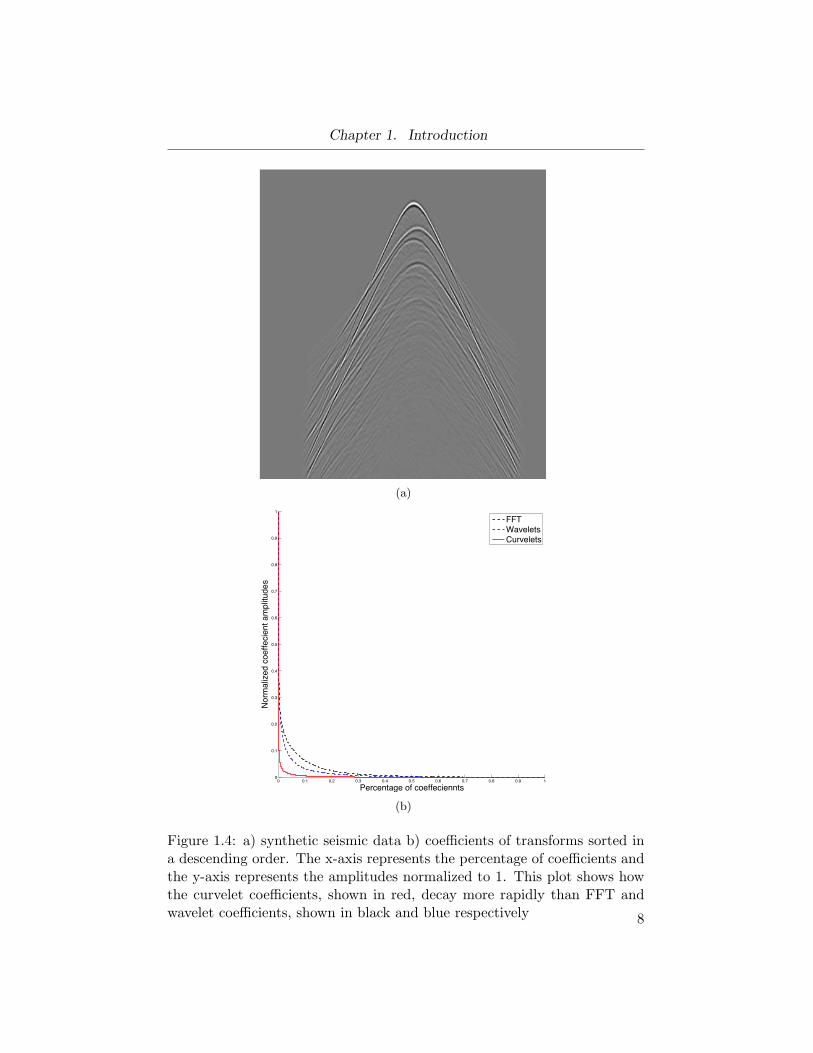
1.4 a) synthetic seismic data b) coefficients of transforms sortedin a descending order. The x-axis represents the percentage ofcoefficients and the y-axis represents the amplitudes normal-ized to 1. This plot shows how the curvelet coefficients, shownin red, decay more rapidly than FFT and wavelet coefficients,shown in black and blue respectively . . . . . . . . . . . . . . 8

2.1 a) Noise free data b) same data from a with added Gaussiannoise with σ = 1.4 c) data after noise removal using SPGL1and the curvelet domain . . . . . . . . . . . . . . . . . . . . . 15

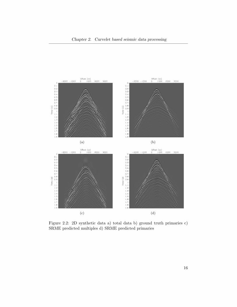
2.2 2D synthetic data a) total data b) ground truth primaries c)SRME predicted multiples d) SRME predicted primaries . . 16

2.3 2D synthetic data a) total data b) ground truth primariesc) SRME predicted primaries d) Our bayesian estimated pri-maries . . . . . . . . . . . . . . . . . . . . . . . . . . . . . . . 17

3.1 a) a centered wrapping curvelet b) the same wrapping curveletlocated near the border. Notice how the curvelet wraps to theopposite border. . . . . . . . . . . . . . . . . . . . . . . . . . 21

ix

List of Figures

3.2 Spectral leakage a) a periodic function on the left and itsFourier transform on the right. b) an aperiodic function onthe left and its Fourier transform on the right. c) differentwindow functions d) The aperiodic function from (b) aftermultiplying by the second window function from c), and itsFourier transform on the right. We can see that applying thewindow function reduces spectral leakage . . . . . . . . . . . 22

3.3 Three tapering windows with two overlapping regions. Theoverlapping region is 2ε wide. We can see the tapering func-tions being 1 everywhere except at the overlapping regionwhere the sum of their square produces 1. The red dashedline represent that quadratic sum. . . . . . . . . . . . . . . . 23

3.4 A simplified illustration of how overlapping and tapering wouldlook like in 3D. . . . . . . . . . . . . . . . . . . . . . . . . . . 23

3.5 Windowing and tapering operators illustrated. Solid lines arewindows boundaries. Dotted lines are overlapping regions.The overlapping region is of width 2ε. . . . . . . . . . . . . . 25

3.6 Scalability plot showing timing of a single forward curvelettransform. The x-axis represents the number of blocks trans-formed in parallel. The y-axis is the time it takes to applythe forward transform including the time it takes to windowand taper the blocks. The red stars are the actual times forour experiments. . . . . . . . . . . . . . . . . . . . . . . . . . 28

3.7 The Forward curvelet transform complexity. Comparing thetime complexity for applying the forward transform on a sin-gle block of data of size M (in blue, M=1536X512X256)withthe time complexity of applying the forward transform on nblocks of size N (in red, N=128X128X128 and n=96) whereN < M. . . . . . . . . . . . . . . . . . . . . . . . . . . . . . . 29

3.8 The two compared scenarios, the dashed red line represent theBayesian solver. Scenario A) Applying the Bayesian separa-tion at each window separately. Scenario B) Emulating theseparation as if the data was not windowed by exchangingedge information between windows. . . . . . . . . . . . . . . 30

4.1 a) Noise free data b) same data from a with added Gaussiannoise with σ = 1.4 c) Denoised data using Scenario A d)Denoised data using Scenario B . . . . . . . . . . . . . . . . 39

x

List of Figures

4.2 2D synthetic data a) total data b) SRME predicted multiplesc) SRME predicted primaries d) estimated primaries usingBayesian separation . . . . . . . . . . . . . . . . . . . . . . . 40

4.3 2D synthetic data a) total data b) true ’multiple-free’ pri-maries c) SRME predicted primaries d) estimated primariesusing Bayesian separation. . . . . . . . . . . . . . . . . . . . 41

4.4 Estimated primaries a) illustration of how data will be di-vided, red lines are window edges. b) applying the Bayesianseparation without any overlapping, tapering or edge updates.Notice the introduced artifacts along the edges indicated bythe pointer. c) Scenario A (no edge updates) with overlapε = 15 d) Scenario B (edge updates) with overlap ε = 15 . . . 42

4.5 Estimated primaries a) illustration of how data will be di-vided, red lines are window edges. b) applying the Bayesianseparation without any overlapping or tapering. Notice theintroduced artifacts along the edges indicated by the pointer.c) Scenario A (no edge updates) with overlap ε = 15 d) Sce-nario B (edge updates) with overlap ε = 15 . . . . . . . . . . 43

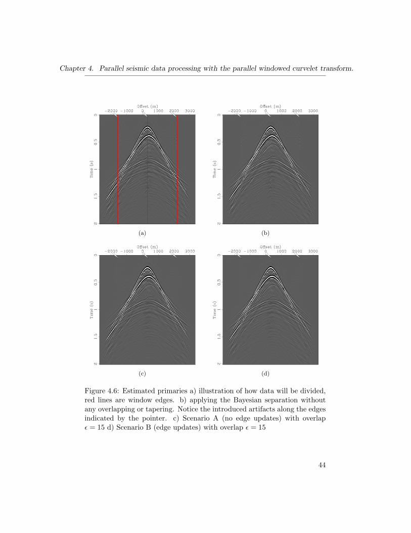
4.6 Estimated primaries a) illustration of how data will be di-vided, red lines are window edges. b) applying the Bayesianseparation without any overlapping or tapering. Notice theintroduced artifacts along the edges indicated by the pointer.c) Scenario A (no edge updates) with overlap ε = 15 d) Sce-nario B (edge updates) with overlap ε = 15 . . . . . . . . . . 44

4.7 Wide vs tall windows. a) tall windows without overlap andtapering b) wide windows without overlap and tapering. Thered ovals highlight some artifacts. . . . . . . . . . . . . . . . . 45

4.8 A closer look of the estimated primaries generated using 16windows and a) no overlap nor tapering b) applying ScenarioA c) applying Scenario B. The images were clipped to 0.8 tomake comparision easier. . . . . . . . . . . . . . . . . . . . . . 46

4.9 A slice from our synthetic 3D data cube. a) Estimated pri-maries using Bayesian separation without windowing. b) Es-timated primaries after windowing into 4X4X2 windows with-out overlaps or tapering. c) Estimated primaries using Sce-nario A (no edge update) d) Estimated primaries using Sce-nario B (window edges exchange information) . . . . . . . . . 47

xi

Preface

This thesis was prepared with Madagascar, a reproducible research soft-ware package available at rsf.sf.net.

A large amount of code was developed in the Seismic Laboratory forImaging and Modeling (SLIM). The numerical algorithms and applicationsare mainly written in Python. with a few experiments written in Matlab.Early experiments were conducted using SLIMpy (slim.eos.ubc.ca/SLIMpy)a Python interface that exploits functionalities of seismic data processingpackages, such as MADAGASCAR, through operator overloading.

xii

Acknowledgments

I would like to thank my supervisor Felix Herrmann for his supportand guidance to make this thesis possible. Also, I would like to thankevery member of the SLIM team for being extremely helpful and providinginformation and help whenever needed.

I am very fortunate to have Michael Bostock and Doug Oldenburg aspart of my supervisory committee. They provided me with some of themost insightful courses I have ever had.

I would like to thank my Management at Saudi Aramco who gave methe chance to study at UBC and provided support and help. They havefunded and sponsored me throughout my studying period at UBC.

I would like to especially thank my wife Ghadeer who helped me duringmy studies at UBC and was my biggest motivator. She provided me withthe strength to acheive my goals and keep going. I also cannot thank myparents enough for encouraging me to continue my quest for knowledge. Aspecial thanks also go to my brother and my sisters.

Finally, I will not forget my best friends that have always stood by myside, especially Maitham Alhubail and Abdullah Alnajjar.

Thank you all.

xiii

To my parents.

xiv

Chapter 1

Introduction

In the early days of oil discovery, petroleum exploration was simply amatter of predicting the subsurface geology based on simple surface obser-vations of signs such as seeps of oil or land formations related to salt domesand other basic observations. Not every prediction was accurate enough butit was a good start. Then, seismology came into the picture and improvedthe discovery in areas with less surface observations. The discovery was rel-atively easy and most of the simple structural traps have been discovered.Since then, geophysicists spent a considerable effort in developing and im-proving scientific methods of processing seismic data that gave huge successin targeting even more complex reservoirs.

Today, as we explore new regions, we face even more complex reservoirsto be discovered that consist of extremely thin strata or are very conformableto the surrounding strata. Such reservoirs may not be able to show on basicseismic data, they require the highest resolution possible. An added com-plexity to the problem is the fact that seismic data contain noise, ghosting,multiples and other kinds of events that obscure thin layers and complexstructures in a seismic image. Such added noise and other undesired eventsdo not completely destroy main features in images of basic structures. Buta small amount of interfering coherent events can make a difference betweenfinding an oil reservoir in a very complex subsurface structure and makingprofit, and, missing the target and losing millions of dollars. This is one ofthe major motivations in the oil industry to denoise complex seismic dataand attenuate multiples (demultiple) or eliminate them (Ikelle and Amund-sen, 2005).

Two major seismic events will be discussed in the coming chapters thatare involved in the process of obtaining higher quality seismic images, specif-ically, in the process of surface-related multiple elimination. These eventsare primaries and multiples. Primaries are seismic events that have beenreflected once before arriving at the receivers (or geophones). Primariesrepresent information about reflectors we are interested in that show thestructure of subsurface. Since we are sending sound waves, any discontinu-ity (boundary, reflector...) in the path of these waves causes the wave to be

1

Chapter 1. Introduction

transmitted and reflected, which means that the recorded seismic data notonly contain events that are reflected once but it contains events generatedby waves traveling many possible paths before being recorded at seismic re-ceivers. We call events that has been reflected more than once between theenergy source and the receivers, multiples. Figure 1.1 shows a syntheticexample of primaries and surface-related multiples. On the top a diagramshowing the waves’ paths and below is the seismic data.

(a)

Figure 1.1: Synthetic data consisting of three primaries and six surfacerelated multiples. Top: the waves paths. Bottom: seismic data of thewaves above. Notice that primaries reflect once while multiples reflect morethan once resulting in some false horizons or reflectors on the seismic image.Adapted from Ikelle and Amundsen, 2005

As mentioned earlier, multiple attenuation or elimination (Verschuuret al., 1992) is an important part of seismic data processing and the processbecomes complex with the presence of noise and other events. There is alsothe fact that seismic data can be incomplete due to physical or economical

2


factors. Many algorithms have been developed in the past, and still are, thataim to enhance seismic images with the available data by removing noiseand filling in missing traces.

Seismic data is well known to be extremely large, and when this datais pre-processed data, the size becomes especially enormous and exceedstoday’s single computer memory (can easily exceed terabytes) which placesa challenge on processing the data. To address this issue, it has always beenpart of seismic data processing to find the most efficient algorithm to dealwith such huge amount of data without losing quality. In addition to findingefficient algorithms, parallelism is an obvious choice for handling huge datain any problem requiring more memory than a single computer can handle.

1.1 Theme

The main theme of this thesis is to utilize a robust technique for mul-tiple elimination based on well-established sparsity-promoting methods andto make this method scalable to realistically sized data. The multiple elimi-nation technique uses the redundant curvelet transform as a sparsifying do-main. This redundancy , in conjunction with the large size of seismic datamakes it impossible to fit seismic data in a single processing unit memory.To overcome these limitations, we design windowing schemes that distributethe data to multiple computing nodes such that it can fit in memory and runthe algorithm with minimal quality loss. The trade-off between the imagequality and running time is investigated.

1.2 Objectives

We have two main objectives: First, to allow a memory demandingiterative multiple elimination method to be applied to a large data set bydividing the data into smaller windows that fit in memory without losingdata quality. Second, to compare two scenarios of using our windowingscheme in which, neighbor windows communicate and exchange information.The two scenarios are:

• Scenario A: Communication between windows occur at the window-ing stage and in the final gathering stage only. After creating thewindows and scattering the windowed data to different nodes, we runour primary-multiple separation on each window separately. This sce-nario has the advantages of simple implementation and fast running

3


time. But since we process each window separately we may lose datacontinuity and accuracy.

• Scenario B: Communication between windows occurs whenever thereis a transform of the data to and from a sparse domain that assumescontinuous data. In this scenario, we try to minimize the effect ofpartitioning our data by defining the sparsifying operator for eachwindow such that they form an overlapping block diagonal operator.This scenario has the advantage of accuracy, but is more complex toimplement and consumes a considerable amount of processing time inI/O to exchange information between windows.

Table 1.1 summarizes the advantages and disadvantages of the abovescenarios.

We will test our windowing methods by applying the above scenariosto a seismic denoising problem. Then, we will apply the scenarios on ourprimary-multiple separation method.

Advantages DisadvantagesScenario A - speed - less accurate

- ease of implementationScenario B - accuracy - complex to implement

- slow runtime (I/O between windows)

Table 1.1: Advantages and disadvantages of Scenario A: windowing data andapplying separation seperatly, Scenario B: windowing data with overlappingoperators.

1.3 Outline

The first chapter introduces the subject of high quality seismic imagingand the need to devise robust techniques to eliminate multiples. It contains abrief discussion on the concept of sparse data representation and introducesthe curvelet transform used to represent seismic data sparsely.

In Chapter 2, we describe the denoising problem that we will use to testour technique. Then, we discuss a new development in wavefield separationby sparsity promotion (Saab et al., 2007; Wang et al., 2008) and explain the

4


basic idea behind the use of curvelets in our Bayesian formulation for theprimary-multiple separation problem.

Chapter 3 introduces our windowing method to resolve the issue of scal-ability that makes it hard to process large seismic data in the redundantcurvelet domain. Such windowing also allows us to process data in parallel.We compare two scenarios where we apply windowing and try to highlighttrade-off between these two scenarios. Finally, we conduct several experi-ments on synthetic data starting with solving a seismic denoising problem,then, applying our windowing methods to our primary-multiple seperationmethod. The results are discussed in Chapter 4.

1.4 Theoretical background

In the world of seismic data processing, we are faced with many differentchallenges, one major challenge is the fact that we are trying to obtain a highquality image of the subsurface of the earth from a set of data that is noisyand incomplete due to physical and economical restrictions. There is alsothe fact that seismic data has bandwidth-limited wavefronts that come inmany shapes, vary in frequency and directions and may contain conflictingdips and caustics (Herrmann and Hennenfent, 2008).

One of the most effective ways to face the above challenges is to workwith seismic data in a sparse domain, which means that we transform thedata to a domain that decomposes data into a form where most of the energyis concentrated in a small number of significant coefficients. This makes thedenoising and primary-multiple separation problems simpler as we can workwith a small set of coefficients that carry the most important energy fromthe data. In the case of data contaminated with white Gaussian noise, agood choice of transform will distribute the random noise into smaller lesssignificant coefficients (Herrmann and Hennenfent, 2008; Hennenfent andHerrmann, 2008; Starck et al., 2002).

For a long time, seismologists have focused on exploiting the Fouriertransform, which decomposes the seismic data into the sum of harmonicwaves that have different frequencies. But the Fourier transform still hassome shortcomings, it assumes that the wave fronts it is representing areplane monochromatic waves and it requires a large number of Fourier co-efficients to represent wavefronts in seismic data. One way to over comethe problem of representing wavefronts, is the use of the wavelet transform,which is a multi scale transform that produces localized coefficients. Butwavelets do not have the sense of direction when it comes to two or higher

5


dimensional data, which means it cannot detect directional information onthe wavefronts (Herrmann and Hennenfent, 2008).

Recently, the curvelet transform (Candes et al., 2006; Ying et al., 2005)was introduced and have successfully resolved the shortcomings mentionedabove in the Fourier and wavelet transforms (Herrmann and Hennenfent,2008). What makes the curvelet transform successful is the fact that curveletsare localized multi scale and multi-directional, they look like localized planewaves that are oscillating in one direction and smoothly varying in the per-pendicular direction. Figure 1.2 shows four curvelets in the spatial andfrequency domain, all of these curvelets have the same angle but differentscales. They are arranged from coarsest to finest scale from left to right.notice that they are localized in the frequency domain. Curvelets follow aparabolic scaling principle, i.e. a curvelet’s length and width are related ac-cording to length = width2. The number of angles in the transform doublesevery other scale. Without prior information, curvelets can find the locationand direction of a wave front when a wave front and a curvelet that have thesame direction and frequency content produce a large inner product betweenthem (Herrmann and Hennenfent, 2008), this is illustrated in Figure 1.3.

One way to show how efficiently a sparse transform represent data isto take the data into the transform’s domain and sort the coefficients in adescending order. This shows how rapid the coefficients decay. The rapiddecay means that we can represent our data with few large coefficients.Fig. 1.4(b) shows a set of sorted coefficients of a synthetic seismic data inthe Fourier, wavelet and curvelet domains. The x-axis represent the per-centage of the number of coefficients and the y-axis shows the coefficientsamplitude. We can see clearly that the curvelet domain has the fastet decay-ing rate. This means that the same seismic data can be represented with asmaller percentage of curvelet coefficients compared to wavelets and Fouriercoefficients.

The fact that the curvelet transform represent seismic data in a smallnumber of large coefficients that are parameterized by location, scale andangle, makes it unlikely for primaries and multiples to overlap. This makesit possible to successfully attempt to develop robust multiples attenuationalgorithms. The computational complexity of the curvelet transform fora data of size M is O(M log M) and is not a major issue. However, thecurvelet transform is an overcomplete signal representation and is 8 timesredundant in 2D and 24 times redundant in 3D. This, in conjunction withthe large size of seismic data, are the motivation for processing in parallel(Thomson et al., 2006).

6


(a)

(b)

Figure 1.2: Four curvelets with the same angle but different scales startingfrom coarsest scale to finest scale left to right in the a) spatial domain b)Fourier or frequency domain

50 100 150 200 250 300

50

100

150

200

250

300

350

400

450

500

significant curvelet coefficient

curvelet coefficient 0

(a)

Figure 1.3: Principle of alignment. Curvelets and wavefronts that locallyhave the same frequency content and direction produce large inner products(significant coefficients). Adapted from Herrmann and Hennenfent, 2008.

7


(a)

0 0.1 0.2 0.3 0.4 0.5 0.6 0.7 0.8 0.9 10

0.1

0.2

0.3

0.4

0.5

0.6

0.7

0.8

0.9

1

Percentage of coeffeciennts

Norm

aliz

ed c

oeffecie

nt am

plit

udes

FFTWaveletsCurvelets

(b)

Figure 1.4: a) synthetic seismic data b) coefficients of transforms sorted ina descending order. The x-axis represents the percentage of coefficients andthe y-axis represents the amplitudes normalized to 1. This plot shows howthe curvelet coefficients, shown in red, decay more rapidly than FFT andwavelet coefficients, shown in black and blue respectively 8

Bibliography


Hennenfent, G. and F. J. Herrmann, 2008, Simply denoise: wavefield re-construction via jittered undersampling: Geophysics, 73, no. 3.

Herrmann, F. J. and G. Hennenfent, 2008, Non-parametric seismic datarecovery with curvelet frames: Geophysical Journal International, 173,233–248.

Ikelle, L. T. and L. Amundsen, 2005, Introduction to petroleum seismology(investigations in geophysics, no. 12): Society of Exploration Geophysicists.

Saab, R., D. Wang, O. Yilmaz, and F. J. Herrmann, 2007, Curvelet-basedprimary-multiple separation from a Bayesian perspective: SEG TechnicalProgram Expanded Abstracts, 2510–2514, SEG.

Starck, J.-L., E. J. Candes, and D. L. Donoho, 2002, The curvelet transformfor image denoising: IEEE Transactions on Image Processing, 11, no. 6,670–684.

Thomson, D., G. Hennenfent, H. Modzelewski, and F. J. Herrmann, 2006,A parallel windowed fast discrete curvelet transform applied to seismic pro-cessing: SEG Technical Program Expanded Abstracts, 2767–2771, SEG.




9

Chapter 2

Curvelet based seismic dataprocessing

2.1 Curvelet based denoising

Seismic data come from the field contaminated with various types of noisethat effect the final processed seismic image.

The problem of incoherent noise elimination can be cast into the follow-ing optimization problem:

min ‖x‖1 subject to ‖Ax− b‖2 ≤ σ, (2.1)

where A is sparsifying operator that we choose to be the curvelet synthesisoperator. The vector b is our data with added white Gaussian noise, and thepositive parameter σ is an estimate of the noise level in the data. (van denBerg and Friedlander, 2008).

Figure 2.1 shows a synthetic data set that we will use to illustrate thedenoising problem. Figure 2.1a shows the noise free synthetic data andFigure 2.1b shows the data after adding white Gaussian noise with standarddeviation 1.4.

We solved the above denoising problem using SPGL1 (Berg and Fried-lander, 2007), a solver for large-scale one-norm regularized least squaresproblems. Figure 2.1c shows our denoised output, which has an SNR valueof 9.5. This was obtained after running for only 14 iterations.

We will use the above denoising problem later in this thesis to test op-erators that will be introduced in the next chapter.

2.2 Curvelet based primary-multiple separation

2.2.1 Introduction

Removal of multiples from seismic data is a vital part of producing high-quality seismic images. In this thesis our goal is to successfully eliminate

10

Chapter 2. Curvelet based seismic data processing

multiples from large seismic data in the presence of noise and possibly incom-plete data. Major advances were accomplished in the multiples eliminationarea, e.g., Surface Related Multiple Elimination (SRME) (Verschuur et al.,1992) Predictive multiple elimination methods, such as SRME, consist oftwo steps: The first step is the prediction step, in this step multiples arepredicted from the seismic data. The second step is the separation stepin which primary reflection and noise are separated, this involves predictedmultiples from the first step to be ”matched” with the true multiples in thedata and eventually removed (Verschuur, 2006; Wang et al., 2008).

In some situations, the subsurface produces three dimensional complex-ity on two dimensional data, which causes multiple predictions to be inaccu-rate. An added complication is the possibility of having ghosts, unbalancedamplitudes in multiple predictions (Herrmann et al., 2007a) and incompletedata (Herrmann et al., 2007c). Many attempts have been made to improvethe process of multiple elimination by either producing more accurate predic-tions of the multiples (Herrmann, 2008; Herrmann et al., 2007c; Verschuurand Berkhout, 1997) or by developing more robust separation techniques(Herrmann et al., 2007a).

2.2.2 Bayesian primary-multiple separation by sparsitypromotion

In a recent development, Wang et al., (2008) have introduced a robustBayesian wavefield separation method to improve on the separation bymatching methods. We will use this method as our main multiple elimi-nation technique.

The separation problem is set up as a probabilistic framework. Seismicdata come from the field as a mixture of primaries, multiples, noise and otherrecorded signals. Our main goal is to recover primaries from a mixture ofprimaries and multiples. The following will be our forward model:

b = s1 + s2 + n, (2.2)

where vector b is our total data and s1 and s2 denote the primaries andmultiples respectively. The vector n is white Gaussian noise with each com-ponent being zero-mean Gaussian with standard deviation σ (Wang et al.,2008). We define the SRME predicted multiples as:

b2 = s2 + n2, (2.3)

where n2 is the error in the SRME prediction, which we also assume to be

11


white Gaussian. The primaries can then be written as

b1 = b− b2 (2.4)= s1 + n− n2

= s1 + n1,

We assume that n and n2 are independent (Wang et al., 2008). We canrewrite the unknown signals s1 and s2 as follows

s1 = Ax1 and (2.5)s2 = Ax2,

where A is a sparse domain synthesis matrix, We choose A to be the curveletsynthesis matrix (Candes et al., 2006; Herrmann, 2006; Herrmann et al.,2007b). This gives us the following system:

b1 = Ax1 + n1 (2.6)b2 = Ax2 + n2.

Now, given the SRME predictions b1 and b2, we want to maximize theconditional probability:

P (x1,x2|b1,b2) = P (x1,x2)P (n)P (n2)/P (b1,b2), (2.7)

this is reformulated into the minimization function:

minx1,x2

f(x1,x2) (2.8)

f(x1,x2) = λ1‖x1‖1,w1 + λ2‖x2‖1,w2 + ‖Ax2 − b2‖22 + η‖A(x1 + x2)− b‖2

2,

where x1 and x2 are curvelet coefficients of the primaries and multiples re-spectively. The parameters λ1 and λ2 allow us to input priori informationrelated to the expected sparsity of the estimated primaries and multiplesrespectively. The vectors w1 and w2 are the weights chosen based on em-pirical findings (Herrmann et al., 2007a) to be w1 = max {|ATb2|, ε} andw2 = max {|ATb1|, ε}, where ε is a noise dependant constant. The param-eter η controls the trade-off between coefficients vectors’ sparsity and themisfit between the total data and the sum of the primaries and multiples.Reducing η increases the thresholding operators’ aggressiveness, and increas-ing η reduces the thresholding operators’ aggressiveness. To solve the aboveminimization problem, an iterative thresholding algorithm was derived from

12


Algorithm: Bayesian iterative method for wavefield separation

input: b1,b2,λ1, λ2, η, niterx1 = 0 ,x2 = 0

threshold w1 =λ1|AT b2|

2η

threshold w2 =λ2|AT b1|

2(η+1)

b1 = ATb1

b2 = ATb2

for i = 1 : niter

x1 = b2 −ATAxn2 + b1 −ATAxn

1 + xn1

x2 = b2 −ATAxn2 + η

η+1

(b1 −ATAxn

1

)x1 = x1

|x1| ·max (0, |x1| − |w1|)x2 = x2

|x2| ·max (0, |x2| − |w2|)

end

Table 2.1: The iterative Bayesian wavefield separation algorithm introducedin Wang et al., 2008; Saab, 2008

the work of Daubechies et al. (2004) and so starting from initial estimatesx0

1 and x02 for several iterations, the nth iteration becomes

xn+11 = Tλ1w1

2η

[ATb2 −ATAxn

2 + ATb1 −ATAxn1 + xn

1

](2.9)

xn+12 = T λ2w2

2(1+η)

[ATb2 −ATAxn

2 + xn2 +

η

η + 1(ATb1 −ATAxn

1

)],

where Tu is the element wise soft thresholding defined as

Tui (vi) :=vi

|vi|·max (0, |vi| − |ui|) , (2.10)

13


The above algorithm, shown in Table 2.1, have proved to be a robustmethod for separating coherent sparse signal components. Using an initialprediction with moderate errors as input, the algorithm produces improvedestimates of these predictions. Because the algorithm takes advantage ofthe curvelet domain, the algorithm has fast convergence and gives excellentquality output data(Wang et al., 2008). Figure 2.3 shows an example ofrunning our Bayesian separation on a 2D data set. We ran the separationfor 10 iterations using the parameters {λ∗

1 = 0.8, λ∗2 = 1.2, η∗ = 1.2}. These

parameters values were found empirically. Notice the improvement in theestimated primaries, where we can see less multiples residual.

Table 2.2 shows sensitivity analysis for our Bayesian separation method.The table shows SNR values calculated against the “multiple-free” groundtruth data, which is generated using the same simulation of the total data,only an energy absorbing boundary condition is enforced to prevent the gen-eration of multiples. We can see from these SNR values that our separationtechnique is robust against changes in the control parameters. Parameterscombinations that aggressively over threshold or under threshold are notincluded, since they produce extremely low SNR values.

SNR (dB) {λ∗1, λ

∗2} {2 · λ∗

1, λ∗2} {λ∗

1, 2 · λ∗2} 100 · {λ∗

1, λ∗2}

η∗ 11.49 11.11 11.40 -12 · η

∗ 11.29 10.38 11.15 -2 · η∗ 10.90 11.38 10.81 -

100 · η∗ - - - 10.99

Table 2.2: Calculated SNR of estimated primaries using the Bayesian sep-aration. SNR was calculated against the ground truth “multiple-free” pri-maries.

14


50 100 150 200 250

50

100

150

200

250

(a)

50 100 150 200 250

50

100

150

200

250

(b)

,1

50 100 150 200 250

50

100

150

200

250

(c)

Figure 2.1: a) Noise free data b) same data from a with added Gaussiannoise with σ = 1.4 c) data after noise removal using SPGL1 and the curveletdomain

15


(a) (b)

(c) (d)

Figure 2.2: 2D synthetic data a) total data b) ground truth primaries c)SRME predicted multiples d) SRME predicted primaries

16


(a) (b)

(c) (d)

Figure 2.3: 2D synthetic data a) total data b) ground truth primaries c)SRME predicted primaries d) Our bayesian estimated primaries

17

Bibliography

Berg, E. v. and M. P. Friedlander, 2007, SPGL1: A solver for large-scalesparse reconstruction. (http://www.cs.ubc.ca/labs/scl/spgl1).


Daubechies, I., M. Defrise, and C. De Mol, 2004, An iterative thresholdingalgorithm for linear inverse problems with a sparsity constraint: Commu-nications on Pure and Applied Mathematics, 57, no. 11, 1413–1457.

Herrmann, F. J., 2006, A primer on sparsity transforms: curvelets andwave atoms: Presented at the SINBAD 2006.

——–, 2008, Curvelet-domain matched filtering: SEG Technical ProgramExpanded Abstracts, 3643–3647, SEG.

Herrmann, F. J., U. Boeniger, and D. J. Verschuur, 2007a, Non-linearprimary-multiple separation with directional curvelet frames: GeophysicalJournal International, 170, no. 2, 781–799.

Herrmann, F. J., G. Hennenfent, and P. P. Moghaddam, 2007b, Seismicimaging and processing with curvelets: Presented at the EAGE TechnicalProgram Expanded Abstracts, EAGE.

Herrmann, F. J., D. Wang, and G. Hennenfent, 2007c, Multiple predictionfrom incomplete data with the focused curvelet transform: SEG TechnicalProgram Expanded Abstracts, 2505–2509, SEG.

van den Berg, E. and M. P. Friedlander, 2008, Probing the Pareto frontierfor basis pursuit solutions: Technical Report TR-2008-01, UBC ComputerScience Department.


Verschuur, D. J. and A. J. Berkhout, 1997, Estimation of multiple scat-tering by iterative inversion, part II: Practical aspects and examples: Geo-physics, 62, no. 5, 1596–1611.

18

Bibliography



19

Chapter 3

Parallel windowed seismicdata processing

3.1 Parallel windowed curvelet transform

It is well known that seismic data sets are extremely large and can easilyreach the size of several terabytes. Also, the two dimensional curvelet trans-form is 8 times redundant and the three dimensional transform is 24 timesredundant; this means we will be dealing with 8 times the size of 2D dataand 24 times the size of 3D data. This, in conjunction with the large size ofseismic field data, makes it impossible to directly apply the curvelet trans-form to the full data into memory on a single processing unit. Currently,users are forced to work out of core to process relatively small 3D data sets.

Even though an MPI implementation of the curvelet transform exists(Ying et al., 2005), it has limitations in scalability since the curvelet trans-form is based on the Fast Fourier Transform, which requires large amountsof communication when the data set is distributed on different processingnodes (Thomson et al., 2006). Our sparsity promoting methods requirerepeated evaluation of matrix-vector multiplications, which multiplies theamount of communication required between processing nodes.

A possible scalable solution is to define a windowing operator that di-vides data into smaller manageable windows. Each window is dealt withseparately, and when all windows are processed and ready, they are joined(gathered) to form the final output. This is a practical solution that min-imizes communication between nodes. But it is likely to have problems atthe borders of these windows, such as artifacts, dimming and/or other typesof problems. For instance, problems arise from the fact that we may dividethe data near a point where a curvelet coefficient would be located and sowhen we take the forward curvelet transform, the curvelet wraps aroundto the opposite border of the transformed data block, see Figure 3.1. Thisreduces the quality of our process and may introduce artifacts . Anotherissue is the fact that the curvelet transform is based on the fast Fourier

20

Chapter 3. Parallel windowed seismic data processing

transform, which produces spectral leakage from aperiodic data. Spectralleakage is basically the spreading of the to-be-transformed signal’s energyinto other frequencies. A well known solution is the use of tapering whichis basically multiplying the data by some function that smoothly reducesthe edges’ amplitudes to zero which minimizes discontinuity. This meanswe can improve our windowing operator by adding a tapering operator thataffects the edges of each of the resulting windows. Figure 3.2 demonstratesspectral leakage from a monochromatic sinusoidal wave and shows the effectof a window function and how it limits the leakage.

(a) (b)

Figure 3.1: a) a centered wrapping curvelet b) the same wrapping curveletlocated near the border. Notice how the curvelet wraps to the oppositeborder.

21


0 0.1 0.2 0.3 0.4 0.5 0.6 0.7 0.8 0.9 1−5

−4

−3

−2

−1

0

1

2

3

4

5

Time(s)

f(t)

0 10 20 30 40 50 60 70 80 90 1000

0.5

1

1.5

Frequancy (Hz)

Am

plit

ude

(a)

0 0.1 0.2 0.3 0.4 0.5 0.6 0.7 0.8 0.9 1−5

−4

−3

−2

−1

0

1

2

3

4

5

Time(s)

f(t)

0 10 20 30 40 50 60 70 80 90 1000

0.5

1

1.5

Frequancy (Hz)

Am

plit

ude

(b)

0 20 40 60 80 100 120 140 160 180 2000

0.1

0.2

0.3

0.4

0.5

0.6

0.7

0.8

0.9

1

Hann Window

0 20 40 60 80 100 120 140 160 180 2000

0.1

0.2

0.3

0.4

0.5

0.6

0.7

0.8

0.9

1

Tukey Window

(c)

0 0.1 0.2 0.3 0.4 0.5 0.6 0.7 0.8 0.9 1−2

−1.5

−1

−0.5

0

0.5

1

1.5

2

Time(s)

f(t)

0 10 20 30 40 50 60 70 80 90 1000

0.05

0.1

0.15

0.2

0.25

0.3

0.35

0.4

0.45

Frequancy (Hz)

Am

plit

ud

e

(d)

Figure 3.2: Spectral leakage a) a periodic function on the left and its Fouriertransform on the right. b) an aperiodic function on the left and its Fouriertransform on the right. c) different window functions d) The aperiodicfunction from (b) after multiplying by the second window function from c),and its Fourier transform on the right. We can see that applying the windowfunction reduces spectral leakage

22


We can define our windowing operator to contain controllable overlap-ping regions at the windows’ edges. This means that our forward windowingwill contain information from adjacent windows. These windows will overlapin a region of total width of 2ε. The overlapping regions communicate viathe way our tapering is defined and a suitable way of defining the taperingoperator is by making sure it satisfies the following relation

T21 + T2

2 = 1, (3.1)

where T1 and T2 are overlapping tapering functions applied to adjacentwindows. This relation guarantees that we have partition of unity, where allwindows add up quadratically to one, preserving the system’s energy. Thisallows us to define our windowing operator as a linear operator. Figure 3.3illustrates how our tapering function looks like.

0

0.5

1

1.5

2

εε

(a)

Figure 3.3: Three tapering windows with two overlapping regions. Theoverlapping region is 2ε wide. We can see the tapering functions being 1everywhere except at the overlapping region where the sum of their squareproduces 1. The red dashed line represent that quadratic sum.

!!"

"

!"

#""

#!"

$""

$!"

%"" !!"

"

!"

#""

#!"

$""

$!"

%""

"

"&!

#

#&!

$

$&!

%

(a)

Figure 3.4: A simplified illustration of how overlapping and tapering wouldlook like in 3D.

There are many functions that are suitable for tapering and satisfy the

23


above property (Mallat, 1998). We chose the following simple tapering op-erator:

Tn = sin((N − n)π2(2ε− 1)

), n = {N,N − 1, ..., N − 2ε + 1}. (3.2)

Here, N is the total width of the overlapping windows. Now we have set upour windowing operator with overlapping regions and a tapering operatorapplied to these windows’ edges such that perfect reconstruction is ensuredand energy of the system is preserved since our windowing and taperingoperators satisfy

W*T*TW = I, (3.3)

where W is our windowing operator that divides our data into overlappingregions, and W* is the adjoint windowing operator, which gathers the win-dowed data into one data set, adding the overlapping regions during theprocess. The operators T and T* are our forward and adjoint tapering op-erators respectively. Finally, the matrix I represents the identity matrix.Figure 3.5 illustrates the way our combination of windowing and taperingworks in 2D.

Now we have a windowing operator that permits us to fit a large data setin a distributed memory and perform operations in parallel to speed up ourseparation algorithm. We can define our parallel forward curvelet transformas:

AT = [C]TW. (3.4)

The block diagonal matrix [C] is our forward curvelet transform matrix.Similarly, the parallel inverse curvelet transform can be defined as:

A = W*T*[C*], (3.5)

where the block diagonal matrix [C*] is our inverse curvelet transform ma-trix.

3.2 Parallel windowed curvelet transform usage

We consider two options to incorporate the windowing operator with oursparsity promoting techniques. The first option, we will call scenario A, is toapply the forward windowing operator with overlaps and tapering and then

24


2ε

Tapering function

0

0.5

1

0 0.5 1

Figure 3.5: Windowing and tapering operators illustrated. Solid lines arewindows boundaries. Dotted lines are overlapping regions. The overlappingregion is of width 2ε.

25


process each window independently for the required number of iterationsand once all windows have been processed, we simply apply the adjointwindowing operator.

The second option, we will call scenario B, is to apply the forward win-dowing operator with overlaps and tapering just like in scenario A, only thistime we allow the overlapping edges of the windows to communicate at eachiteration in our process.

In both scenarios we solve a set of nonlinear minimization problems. Forinstance, instead of solving the denoising problem from the previous chapter(Eqn 2.1) as a single system we solve the following set of problems seperatly:

min ‖x1‖1 subject to ‖Ax1 − b1‖2 ≤ σ (3.6)

min ‖x2‖1 subject to ‖Ax2 − b2‖2 ≤ σ (3.7)

min ‖x3‖1 subject to ‖Ax3 − b3‖2 ≤ σ

...min ‖xn−1‖1 subject to ‖Axn−1 − bn−1‖2 ≤ σ

min ‖xn‖1 subject to ‖Axn − bn‖2 ≤ σ

where n is the number of windows. The vectors b1, b2, · · · , bn representour windowed data, where each vector is a window of our n windows. Thevectors x1, x2, · · · , xn represent our denoised outputs. In scenario A, eachinstance of the above problems is solved without communicating with anyother instances, while in scenario B, each instance is solved independentlybut communicates and updates the edges of neighboring windows.

Each of the above two scenarios have advantages and disadvantages. Thefirst scenario has the advantages of simple implementation and reduced I/Otime between nodes. But it only exchanges window edge information atthe very end and might affect the accuracy of our estimation during theseparation iterations. The second scenario insures that the edges have up-to-date information about the region it is overlapping at each iteration. Butthis scenario is complex to implement and requires a considerable amount ofcommunication between nodes. Some of this time is spent by each windowwaiting for all of its edges to be ready before going to the next step in thealgorithm. So for a 2D data set, a central window will be waiting for fourother windows to update edge information and in 3D, a window will waitfor 12 other windows, unlike Scenario A, where all windows work in parallel

26


until the end. Another area time is spent on in Scenario B is the time spentto exchange data between windows which involves plenty of I/O operations.

3.3 Scalability

To test the scalability of our approach, we applied the forward curvelettransform on a 3D cube of size 128X128X128 (shots X traces X time sam-ples). We then compared the time it takes to transform this block withthe time it takes to apply our parallel curvelet transform on a bigger blockwindowed into several 128X128X128 blocks. This ensures a fair comparison,since applying the curvelet transform to different block sizes requires differ-ent processing time. Our testing blocks contained 24, 48, 64 and 96 blocksof size 128X128X128. For instance the 96 blocks composed a bigger block ofsize 1536X512X256. Figure 3.6 shows the results of our experiments. Thex-axis represent the number of blocks transformed in parallel. The y-axis isthe time it takes to apply the forward transform in seconds, including thetime it takes to window and taper the blocks. The red stars are the actualtimes for our experiments. We can see that as we increase the number ofblocks the time it takes to perform the transform naturally increases. Wecan see that it takes 96 blocks about three times the time it takes a singleblock to be transformed which is a very good ratio.

Part of the processing time increase is due to the fact that we have morewindows to extract and more windows to apply tapering on. Also, we needmore I/O operations and file management. The processing time can be fur-ther optimized by optimizing the windowing and tapering implementation,and enhancing I/O and file management techniques.

We also applied a single forward curvelet transform to the largest dataset in our experiments (1536X512X256) without parallelization. It took422 seconds to complete, compared to 123 seconds when using our parallelcurvelet transform on the same data set. This gives a perspective on howmuch speed we can gain with parallelism. Considering the time complexityof O(M log M) for the curvelet transform, Figure 3.7 Compares the timecomplexity for applying the forward transform on a single block of data ofsize M=1536X512X256 with the time complexity of applying the forwardtransform on 96 blocks of size N=128X128X128.

27


0 20 40 60 80 10030

40

50

60

70

80

90

100

110

120

number of blocks

tim

e (

s)

(a)

Figure 3.6: Scalability plot showing timing of a single forward curvelet trans-form. The x-axis represents the number of blocks transformed in parallel.The y-axis is the time it takes to apply the forward transform including thetime it takes to window and taper the blocks. The red stars are the actualtimes for our experiments.

28


0 20 40 60 80 1000

0.5

1

1.5

2

2.5

3

3.5

4x 10

9

M log(M)

n * N log(N)

(a)

Figure 3.7: The Forward curvelet transform complexity. Comparing thetime complexity for applying the forward transform on a single block of dataof size M (in blue, M=1536X512X256)with the time complexity of applyingthe forward transform on n blocks of size N (in red, N=128X128X128 andn=96) where N < M.

29


2D

Data

Scatter with

overlap

+

Sparsity (Curvelet) Based

Separation Taper

+

Gather

2D

3D

3D

Update

Edges

2D

Data

Scatter with

overlap

Sparsity (Curvelet) Based

Separation Taper

+

Gather

2D

3D

3D

Scenario A

Scenario B

(a)

Figure 3.8: The two compared scenarios, the dashed red line represent theBayesian solver. Scenario A) Applying the Bayesian separation at eachwindow separately. Scenario B) Emulating the separation as if the data wasnot windowed by exchanging edge information between windows.

30

Bibliography

Mallat, S., 1998, A wavelet tour of signal processing: Acadamic Press.

Thomson, D., G. Hennenfent, H. Modzelewski, and F. J. Herrmann, 2006,A parallel windowed fast discrete curvelet transform applied to seismic pro-cessing: SEG Technical Program Expanded Abstracts, 2767–2771, SEG.


31

Chapter 4

Parallel seismic dataprocessing with the parallelwindowed curvelettransform.

In this chapter, we put our windowing method in action, compare the twoscenarios defined in the previous chapter and present some findings. First,we tested our windowing technique with a denoising problem and observedour windows edges effect on the solution. Then, we applied our windowingoperators in combination with our Bayesian separation method on 2D and3D data sets. In every experiment, we calculated SNR and compared results.

4.1 Parallel windowed seismic data denoising

We ran multiple experiments using SPGL1 (Berg and Friedlander, 2007)to solve the denoising problem introduced in Chapter 2 using our parallelwindowed curvelet transform, in each experiment, we change a set of pa-rameters, namely, the sparsifying operators, window sizes and overlap sizes.We then calculated the SNR against the noise free data according to :

SNR = 20 log‖ d‖d‖2

‖2

‖ dn‖dn‖2

− d‖d‖2

‖2

, (4.1)

where d denotes our noise free data and dn is our denoised solution.Table 4.1 shows the SNR values from our experiments. The first columnspecifies which scenario was used. Scenario A: solving each window inde-pendently with no edge information update during separation. Scenario B:solving each window independently with edge information updates occur-ring at each iteration. Each pair of rows share the same parameters firstfor Scenario A and second for scenario B. The second column shows the

32

Chapter 4. Parallel seismic data processing with the parallel windowed curvelet transform.

number of windows in each dimension. So for example 2X4 is interpreted asdividing the data into 2 windows along the time axis and 4 windows alongthe receiver axis. We can see that we have three groups based on overlapvalues of 6,10 and 16.

Figure 4.1 shows the noise free data and the data after adding noise onthe top. On the bottom, we can see the two results from scenario A on theleft and scenario B on the right. Both were windowed into 16 equal windows.

Looking at the SNR values in Table 4.1, we notice several points. First,we notice that in each of the scenarios the different window sizes result indifferent SNR values with considerable variations. For example, running sce-nario A with overlap value ε = 16 resulted in SNR values that range between6.89 and 8.11. Another example is the SNR values resulting from scenarioB with ε = 16 that range from 7.26 to 10.34. These variations in SNR aredue to the fact that each time, we are solving a different non-linear problemand when we change the windows’ sizes, we also change the location wherewe divide the data, and hence, the likelihood that significant coefficients arelocated near the edges of the windows or in the overlapping region. Com-paring SNR values from scenario A and B, we notice that scenario B resultsin higher SNR values compared to corresponding values from scenario A.This is due to the overlap in our curvelet transform which minimizes theeffect of dividing the data. The improvement in SNR reached a differenceof up to 2.23 dB, which is a considerable amount of improvement. Someresults showed more improvement than others, because the combinations ofwindow sizes and overlaps affects the data differently in terms of the amountof significant curvelet coefficients near the borders. But in general, scenarioB produced higher SNR values throughout our experiments.

4.2 Parallel windowed primary-multipleseparation

Our set of primary-multiple separation experiments were conducted on syn-thetic data that contained 361 shots, 361 traces/shot, 501 time samples/-trace with sample intervals ∆t = 4ms.

We started by applying our code on shot record number 181 for our 2Dexperiment. Then, applied the code on the 3D dataset using the 3D curvelettransform (Ying et al., 2005). Our input dataset consisted of predicted(SRME) primaries s1 and predicted multiples s2 = d − s1, where d is ourtotal data, and ”multiple free” data sp, which is generated using the samesimulation of the total data, only an energy absorbing boundary condition

33


Scenario Window SNRε = 6

A 1X2 7.30B 1X2 7.70A 2X2 7.39B 2X2 7.90A 1X4 7.80B 1X4 8.16A 4X4 8.06B 4X4 8.27

ε = 10A 1X2 7.90B 1X2 9.35A 2X2 7.73B 2X2 7.91A 1X4 7.04B 1X4 8.05A 4X4 7.94B 4X4 8.12

ε = 16A 1X2 6.89B 1X2 7.26A 2X2 6.97B 2X2 7.38A 1X4 8.11B 1X4 10.34A 4X4 7.02B 4X4 7.50

Table 4.1: Calculated SNR for the denoise problem. The first column speci-fies which scenario was used. Scenario A: no edge information update duringseparation. Scenario B: edge information update occurs at each transformcall. each pair of rows share the same parameters used in scenario A and B.The window column shows the number of windows at each dimension, thesewindows have identical sizes.

34


is enforced to prevent the generation of multiples. The ”multiple free” datawere used as a reference to calculate SNR according to Eqn 4.1.

Figure 4.2 shows the total data, predicted multiples, predicted SRMEprimaries and estimated primaries after applying the Bayesian separation.

4.2.1 2D data experiments

Table 4.3 shows SNR calculated against the true primaries with differentparameters. The first column specifies which scenario was used. The secondcolumn shows the number of windows in each dimension. We can see that wehave three groups based on overlap values of 10,15 and 20. For comparison itis important to mention that the SNR value of the SRME predicted primariesis 9.82, and the SNR of the estimated primaries after applying the Bayesianseparation without any windowing is 11.49.

Looking at Table 4.3 we notice the following: First, we notice that allSNR values in the table are extremely close and unlike the case with thedenoising problem the changes in window sizes for each of the scenarios doesnot have considerable variations in the output SNR values. The differencesbetween the lowest and highest SNR values in scenario A and scenario B are0.07 and 0.079 respectively. This is a major advantage of our Bayesian sepa-ration technique where we threshold the primaries against a fixed thresholdbased on the multiples, and threshold the multiples with a fixed thresholdbased on the primaries. In both cases, the primaries and multiples are win-dowed and tapered. Another reason that explains these results, is the factthat in the denoising problem, the solver uses a cooling method where itstarts with a very sparse solution, this sparseness is translated into a smallnumber of curvelets, if some of this small number is located near windowsedges, they will have distingushable presense and create artifacts. But theBayesian separation works with a large number of coefficients such that theycontribute in reducing the possibility of having artifacts near the windowedges because we have enough curvelets to diminish the effect of wrppingaround the window edges.

We also notice that the more windows we have the lower SNR valueswe get, one reason for this is the fact that we increase the discontinuitiesintroduced in the data and hence the probability of a curvelet being locatednear the borders. Also, notice that as we increase the overlap, we get higherSNR. Because large overlaps allow windows to have more information andbe tapered more smoothly than smaller overlaps.

Our goal is to compare the two scenarios we have. And looking at theSNR values we can see that, as expected, in general Scenario B, which

35


updates windows’ edges, has higher values. But the difference between thetwo scenarios is in the hundredth decimal place, with a maximum of 0.0276,which is considered small.

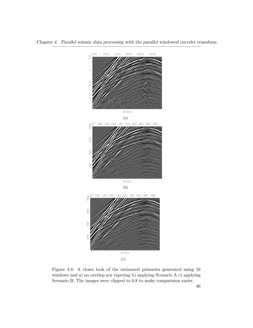
Figure 4.4 shows one of our worst cases where we divide the data into16 equal windows. Figure 4.4b shows the estimated primaries from ourBayesian method after windowing into 16 windows without applying any ta-pering or overlap, we can clearly see introduced artifacts along the windows’edges. Figure 4.4c shows the estimated primaries after applying ScenarioA. We can clearly see that the artifacts are gone now and the data lookscleaner. Same applies to Figure 4.4d, which shows the estimated primariesafter applying Scenario B. Comparing Figure 4.4c and Figure 4.4d we cansee that both results are extremely close and differentiating between themis difficult. This is consistant with the SNR results in Table 4.3. Lookingat different scenarios we get the same observation, i.e. Scenario A performsvery well with very close output to the one from Scenario B. Figuers 4.5and 4.6 also show the same outcome using different windows’ sizes. Thismeans that in terms of SNR and image quality, we can use Scenario A andsave a considerable amount of processing time that is consumed as I/O timebetween processing nodes.

Our experiments with 2D data show that Scenario A produces excellentresults compared to the more complex but relatively more accurate Sce-nario B in the context of our Bayesian separation technique. We furtherinvestigate the two scenarios using 3D data and the 3D curvelet transform.

36


Scenario Window Overlap ε SNR DifferenceA 2X2 10 11.41B 2X2 10 11.43 0.02A 2X3 10 11.46B 2X3 10 11.48 0.02A 3X2 10 11.37B 3X2 10 11.38 0.01A 4X4 10 11.39B 4X4 10 11.41 0.02A 1X4 10 11.40B 1X4 10 11.41 0.01A 4X1 10 11.38B 4X1 10 11.39 0.01

A 2X2 15 11.44B 2X2 15 11.46 0.02A 2X3 15 11.43B 2X3 15 11.46 0.03A 3X2 15 11.39B 3X2 15 11.40 0.01A 4X4 15 11.41B 4X4 15 11.43 0.02A 1X4 15 11.42B 1X4 15 11.43 0.01A 4X1 15 11.40B 4X1 15 11.41 0.01

A 2X2 20 11.44B 2X2 20 11.46 0.02A 4X4 20 11.41B 4X4 20 11.42 0.01

Table 4.2: Calculated SNR for the 2D synthetic data set. The first columnspecifies which scenario was used. Scenario A: no edge information up-date during separation. Scenario B: edge information update occurs at eachtransform call. each pair of rows share the same parameters used in scenarioA and B. The difference column carry the difference between the SNRs ofscenario A and B for each pair. The window column shows the numberof windows at each dimension, these windows have identical sizes. Noticethat the more windows we have the more discontinuities in the data whichlowers the SNR. Also, notice that increasing the overlap amount improvesthe SNR. All results were achieved after 10 iterations of the solver.

37


4.2.2 3D data experiments

The scalability issue we are attempting to solve is more crucial with 3D datasince it requires more memory. We applied the Bayesian separation on oursynthetic 3D data and calculated the SNR for each experiment the same waywe did for 2D data. The SNR value of the predicted SRME primaries is 9.928and the SNR after applying the Bayesian separation without windowing is11.466.

Table 4.3 shows calculated SNR values from our experiments. Just like inthe 2D case we can see that the variations between SNR values are extremelysmall. Scenario B showed relatively higher SNR values than scenario A, yetthe difference is negligible.

Figure 4.9 shows a slice taken from the 3D cube at shot point 181. Fig-ure 4.9a shows the estimated primaries after applying Bayesian separationwithout any windowing. Figure 4.9b shows the estimated primaries afterwindowing, with 4X4X2 windows, without any overlapping nor tapering.Notice the large amount of introduced artifacts, especially around the win-dows’ edges. Figuers 4.9c and 4.9d show the estimated primaries usingscenarios A and B, respectively. Notice that there are almost no artifactsaround windows’ edges. Note that this is one of the worst cases in Table 4.3.

Scenario Window Overlap ε SNR DifferenceA 2X2X2 15 11.50B 2X2X2 15 11.51 0.01A 2X4X4 15 11.50B 2X4X4 15 11.51 0.01A 4X4X2 15 11.46B 4X4X2 15 11.47 0.01

Table 4.3: Calculated SNR for the 3D synthetic data set. The first col-umn specifies which scenario was used. Scenario A: no edge informationupdate during separation. Scenario B: edge information update occurs ateach transform call. each pair of rows share the same parameters used inscenario A and B. The difference column carry the difference between theSNRs of scenario A and B for each pair. The window column shows thenumber of windows at each dimension, these windows have identical sizes.Notice that the more windows we have the more discontinuities in the datawhich lowers the SNR.

38


50 100 150 200 250

50

100

150

200

250

(a)

50 100 150 200 250

50

100

150

200

250

(b)

50 100 150 200 250

50

100

150

200

250

(c)

44

50 100 150 200 250

50

100

150

200

250

(d)

Figure 4.1: a) Noise free data b) same data from a with added Gaussiannoise with σ = 1.4 c) Denoised data using Scenario A d) Denoised datausing Scenario B

39


(a) (b)

(c) (d)

Figure 4.2: 2D synthetic data a) total data b) SRME predicted multiples c)SRME predicted primaries d) estimated primaries using Bayesian separation

40


(a) (b)

(c) (d)

Figure 4.3: 2D synthetic data a) total data b) true ’multiple-free’ primariesc) SRME predicted primaries d) estimated primaries using Bayesian sepa-ration.

41


(a) (b)

(c) (d)

Figure 4.4: Estimated primaries a) illustration of how data will be divided,red lines are window edges. b) applying the Bayesian separation withoutany overlapping, tapering or edge updates. Notice the introduced artifactsalong the edges indicated by the pointer. c) Scenario A (no edge updates)with overlap ε = 15 d) Scenario B (edge updates) with overlap ε = 15

42


(a) (b)

(c) (d)

Figure 4.5: Estimated primaries a) illustration of how data will be divided,red lines are window edges. b) applying the Bayesian separation withoutany overlapping or tapering. Notice the introduced artifacts along the edgesindicated by the pointer. c) Scenario A (no edge updates) with overlapε = 15 d) Scenario B (edge updates) with overlap ε = 15

43


(a) (b)

(c) (d)

Figure 4.6: Estimated primaries a) illustration of how data will be divided,red lines are window edges. b) applying the Bayesian separation withoutany overlapping or tapering. Notice the introduced artifacts along the edgesindicated by the pointer. c) Scenario A (no edge updates) with overlapε = 15 d) Scenario B (edge updates) with overlap ε = 15

44


(a)

(b)

Figure 4.7: Wide vs tall windows. a) tall windows without overlap andtapering b) wide windows without overlap and tapering. The red ovalshighlight some artifacts.

45


(a)

(b)

(c)

Figure 4.8: A closer look of the estimated primaries generated using 16windows and a) no overlap nor tapering b) applying Scenario A c) applyingScenario B. The images were clipped to 0.8 to make comparision easier.

46


(a) (b)

(c) (d)

Figure 4.9: A slice from our synthetic 3D data cube. a) Estimated primariesusing Bayesian separation without windowing. b) Estimated primaries afterwindowing into 4X4X2 windows without overlaps or tapering. c) Estimatedprimaries using Scenario A (no edge update) d) Estimated primaries usingScenario B (window edges exchange information)

47

Bibliography

Berg, E. v. and M. P. Friedlander, 2007, SPGL1: A solver for large-scalesparse reconstruction. (http://www.cs.ubc.ca/labs/scl/spgl1).


48

Chapter 5

Conclusion

5.1 Parallel curvelet domain seismic dataprocessing

Our goal in this thesis is to solve the problem of scalability of the curvelettransform in iterative seismic processing techniques such as the combina-tion of SRME (Verschuur et al., 1992) and Bayesian separation used in(Verschuur, 2006; Wang et al., 2008). We have introduced a windowingtechnique that allows us to divide large seismic data into smaller data setsthat make it possible to fit the huge data and redundant curvelet coefficientsinto memory. Since we divide the data, we introduce discontinuities at thewindows’ edges, hence, we need to address the issue of curvelet coefficientslocated at the boundaries of these windows. We applied a window taperingfunction to our windowing operator. We designed the windows to overlapsuch that the sum of the tapered overlapping regions preserve the system’senergy. Once we had a windowing operator we compared two scenarios ofapplying it on our denoising and multiple elimination problems. The firstscenario divides the data with our windowing operator and then processeach window independently. Finally, when each window is processed, theadjoint windowing is applied and the final data set is gathered. The secondscenario redefines the sparsifying operator such that it allows the windowsto be independently processed but update their overlapping edges.

The advantages of using the first scenario are simplicity in implemen-tation and speed. There is minimum I/O time between the windows. Themain advantage of the second scenario is accuracy. But this scenario spendsa considerable amount of time in I/O. Not only does the edge informationexchange consume time, but each window has to wait for all neighboringwindows to finish before updating.

From our experiments, the second scenario showed a considerable advan-tage when solving the denoising problem. Our Bayesian separation showedextremely small differences between the two scenarios and showed the ad-vantage of allowing us to use the faster and simpler windowing technique

49

Chapter 5. Conclusion

without losing considerable degree of accuracy.

5.2 Open and future research

The use of curvelets (Candes et al., 2006) as a sparsifying domain in seismicimaging has opened great opportunities in geophysical applications suchas seismic image regularization, ground roll removal and primary multipleseparation (Yarham et al., 2007; Herrmann, 2008; Yan, 2008; Hennenfentand Herrmann, 2005, 2006).

Our application of curvelets on primary-multiple separation is based ongeneral sparsity concepts. This gives the chance to experiment with differ-ent sparsifying domains that might come up in the future. Another possibleresearch area would be to develop an automated way to choose parametersin our algorithms, such as curvelet parameters (e.g. scale, angle) and win-dowing parameters such as window dimensions and the amount of overlap.Also, the protocols, by which our method manages data and I/O can beconsidered as a good area for improvement.

50

Bibliography


Hennenfent, G. and F. J. Herrmann, 2005, Sparseness-constrained datacontinuation with frames: applications to missing traces and aliased signalsin 2/3-D: SEG Technical Program Expanded Abstracts, 2162–2165, SEG.

——–, 2006, Application of stable signal recovery to seismic data interpo-lation: SEG Technical Program Expanded Abstracts, 2797–2801, SEG.

Herrmann, F. J., 2008, Adaptive curvelet-domain primary-multiple sepa-ration: Presented at the SINBAD 2008. (SINBAD 2008).




Yan, J., 2008, Wavefield reconstruction using simultaneous denoising in-terpolation vs. denoising after interpolation: Presented at the SINBAD2008.

Yarham, C., G. Hennenfent, and F. J. Herrmann, 2007, Curvelet applica-tions in surface wave removal: Presented at the EAGE Technical ProgramExpanded Abstracts, EAGE.

51

seismic data processing with the parallel windowed ... · pdf fileseismic data processing with...

Documents