JOURNAL OF GEOPHYSICAL RESEARCH, VOL. 102, NO. B5, PAGES 9949-9960, MAY 10, 1997

Seismic attribute inversion for velocity and attenuation structure using data from the GLIMPCE Lake Superior experiment

Michael P. Matheney and Robert L. Nowack Department of Earth and Atmospheric Sciences, Purdue University, West Lafayette, Indiana

Anne M. Tr•hu

College of Oceanic and Atmospheric Sciences, Oregon State University, Corvallis

Abstract. A simultaneous inversion for velocity and attenuation structure using multiple seismic attributes has been applied to refraction data from the 1986 GLIMPCE Lake Superior experiment. The seismic attributes considered include envelope amplitude, instantaneous frequency, and travel time of first arrival data. Instantaneous frequency is converted to t* using a matching procedure which approximately removes the effects of the source spectra. The derived seismic attributes are then used in an iterative inversion procedure referred to as AFT inversion for amplitude, (instantaneous) frequency, and time. Uncertainties and resolution of the velocity and attenuation models are estimated using covariance calculations and checkerboard resolution maps. A simultaneous inversion of seismic attributes from the GLIMPCE data results in a velocity model similar to that of previous studies across Lake Superior. A central rift basin and a northern basin are the most prominent features with an increase in velocity near the Isle Royale fault. Although there is an indication of the central and northern basins in the attenuation model for depths greater than 4 km, the separation is not evident for shallower depths. This may result from microfractures masking compositional variations in the attenuation model for shallower depths. Attenuation Q values range from approximately 60 near the surface to near 500 at 10 km depth. A relationship between inverse Q and velocity of Q'•=0.0210-0.0028*v was found with a correlation coefficient of-0.96. This suggests a nearly linear, inverse relationship between Q.l and velocity beneath Lake Superior which supports previous laboratory results. The inverted velocity and attenuation models provide important constraints on the lithology and physical properties of the Midcontinent rift beneath Lake Superior.

Introduction

The Midcontinent rift (MCR) is a 1.1 Gyr old feature which extends from Kansas up through Iowa, Minnesota, Lake Superior, and into Michigan. The study of the MCR is important for understanding rifting processes and reactivation of ancient rifts. The MCR is also of interest because of its

hydrocarbon potential [Dickas, 1984] and mineral wealth [LaBerge, 1994]. Gravity studies first revealed the MCR [Woolard, 1943; Hinze et al., 1975] and continue to provide insight into the rift's development [Allen, 1994]. The magnetic properties of the volcanic rocks have also been useful in determining the rift's evolution [Hinze et al., 1966; Chandler et al., 1989; Mariano and Hinze, 1994].

The most detailed images of the MCR have come from seismic reflection and refraction profiles. Seismic reflection surveys provide the highest resolution of the rift basin. Substantial crustal reflections come from contrasts between

volcanic flows and sedimentary rocks [Behrendt et al., 1988; Cannon et al., 1989; Chandler et al., 1989]. Additional seismic reflectors result from composition changes within the

Copyright 1997 by the American Geophysical Union.

Paper number 97JB00332. 0148-0227/97/97JB-00332509.00

sedimentary units. The refraction surveys provide valuable information on the velocity structure and lithology of the rift basin and underlying rocks. Early seismic refraction investigations by Berry and West [1966], Steinhart and Smith [1966], and Halls [1982] imaged lower velocities associated with the upper sedimentary rocks, higher velocities associated with the underlying volcanic rocks, and a thickening of the crust beneath the MCR. More recent tomographic imaging and forward modeling studies [Trdhu et al., 1991; Lutter et al., 1993; Hamilton and Mereu, 1993] have delineated the thickened crust, central and northern rift basins, an increase in velocity around the Isle Royale fault, and higher velocities associated with lava flows and intrusives.

In general, there have been fewer studies of in situ attenuation compared to studies of velocity [Carpenter and Sanford, 1985; Brzostowski and McMechan, 1992]. This is mostly due to the difficulty in accurately measuring seismic attributes used to estimate in situ seismic attenuation.

Laboratory measurements of rocks, however, have provided information on the attenuation associated with certain rock

types [Toks6z et al., 1979; Wepfer and Christensen, 1991; Best et al., 1994]. These laboratory attenuation estimates are typically made at seismic frequencies in the megahertz range, and it is not clear how these values relate to attenuation at

frequencies used in seismic refraction studies [Goldberg and Yin, 1994]. Some attenuation studies have used frequency-

9949

9950 MATHENEY ET AL.: SEISMIC ATTRIBUTE INVERSION

92 ø

..I i,'•/i'

48 ø '.-'",'

4T

i I

90 ø 88 ø 86 ø

I -:- . ''':-: : ' : ',',•mu, .R •- ':- /_- /.• .' '.,., ':

,-•.•,.,.,•, ,. ,.-,-,-,.'• ...

,-,?,-,.•.'.- •.,.,., ,,'_q • -' '.'5 .... 2, •, ',',-,-;-7 • ,'. :•1 ,' Vz, :, ,,-,.-,- , ", ',:; ",-,-; -7'-' •-'/•,•• - - ','z

'•c: ' ' '•'"' ., . .•...•,•2• •½•,,. ,-, •'"••••••• ?-•;."".. • _ ,'., ß .. • .c•-'/' •Z 1• • 70.

I•111111••'.•, •, ' • G o • ' • ' • roc•

..... ..... ..;/ , i

EXPLANATION

Upper Keweenawan sedimentary rocks (Bayfield Group and Jacobsville Sandstone)

Upper Keweenawan sedimentary rocks (Oronto Group) Middle Keweenawan (Basalt flows and sedimentary rocks/Gabbroic intmsives) Lower Keweenawan

(Basalt flows and underlying sedimentary rocks)

Lower Keweenawan? (Sibley Group)

Archean and Lower Proterozoic crystalline rocks

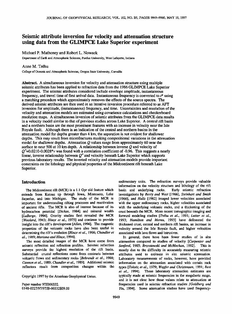
Figure 1. Map of the Lake Superior area showing the probable lithologies and the location of line A of the GLIMPCE experiment. Seismometer locations S4 and C1 are land-based seismometers and A2, C4, C9, and C3 are lake bottom seismometers. The dashed line shows the axis of the Midcontinent rift (MCR). (Geology adapted from Cannon et al., [1989])

independent attenuation operators [Futterman, 1962; Kjartansson, 1979] to estimate attenuation [Johnston, 1981], while other studies have used frequency-dependent Q mechanisms [Mason et al., 1978]. In all cases, in situ estimates of attenuation are important for the interpretation of the physical state of the subsurface [ToksOz et al., 1979]. In situ attenuation estimates can also be used in seismic reflection data

processing to provide improved images of the subsurface [Sollie and Mittet, 1994; Brzostowski and McMechan, 1992].

This study uses seismic refraction data from the 1986 Great Lakes International Multidisciplinary Program on Crustal Evolution (GLIMPCE) experiment. Part of the GLIMPCE experiment included the recording of a 250 km long, wide- angle refraction profile which extended across Lake Superior from north to south (Figure 1). Data were recorded by four lake bottom and two land-based seismometers.

The seismic attributes used in this study include envelope amplitude, instantaneous frequency, and travel time of the first arrivals. The instantaneous frequencies are converted to t* by using a matching procedure given by Matheney and Nowack [1995] which approximately removes the effects of the source spectra. The trace attributes are then utilized in an iterative, inversion procedure which simultaneously images the subsurface velocity and attenuation structure. This is referred to as AFT inversion for the attributes amplitude, (instantaneous) frequency, and time. Uncertainty and resolution estimates are obtained through covariance calculations and checkerboard resolution plots.

Geologic Overview

The crustal rocks imaged using the GLIMPCE reflection and refraction data are rift volcanics and sediments of middle

Proterozoic (~1.1 Ga) age. At the start of this rifting event, upwelling of mantle material caused doming across the Lake Superior region [Allen et al., 1992; Cannon and Hinze, 1992]. Resulting extensional forces, due to the uplifting, initiated rifting. The earliest flood basalts covered large areas in and adjacent to the central rift with flows varying in thickness from several meters to over 100 m [Green, 1989]. During the time of volcanism, 1109 Ma to 1084 Ma, periods of quiescence allowed for deposition of sandstones and conglomerates between the lava flows. Further subsidence during volcanism, especially along the central rift, allowed lava flows to accumulate up to 19 km in thickness [Behrendt et al., 1988; Cannon et al., 1989]. This sequence of volcanic and sedimentary rocks is called the Portage Lake Volcanic sequence.

As the igneous activity decreased along the rift around 1089 Ma, the deposition of sediments became the dominant rock- forming activity. The Oronto Group is a large sequence of sedimentary rocks, with intermittent basaltic flows, which overlies the volcanic rocks around Lake Superior. These sediments are similar in composition to the volcanic flows, indicating that a significant part of the original basaltic lava flows was eroded to form the Oronto Group. The Oronto group has a maximum thickness of about 8000 m near the center of

the rift basin. The Bayfield Group is a younger, undeformed

MATHENEY ET AL.: SEISMIC ATI'RIBUTE INVERSION 9951

1.7-

0.8-

O0 -60.0 -•,9.2 -38.3 -27.5 -16.7 -5.8 5.0 15.8 26.7 37.5 •,8.3 59.2

Distance (km)

Figure 2. GLIMPCE Lake Superior record section A2 with amplitudes for each trace normalized by the maximum amplitude over a 0.4 second window after the first arrival. Every fifth trace is plotted.

sequence of sandstones. These sandstones vary up to 2000 m in thickness [Halls and West, 1971] and did not undergo the tilting and warping associated with the Lake Superior Syncline.

The Grenville Orogeny subjected the MCR to compressional forces which caused thrust faulting and horst development. These faults include the Keweenaw fault, Isle Royale fault and the St. Croix Horst. With the uplift associated with faulting, some reworking of earlier sediments occurred. This was the last significant rock-forming episode in the Lake Superior region.

Data Analysis

The initial data analysis of this study required the extraction of seismic trace attributes, travel time, amplitude, and instantaneous frequency, from the seismic record sections. Seismic attenuation caused by intrinsic attenuation, as well as scattering, in the subsurface results in a loss of amplitude as well as a lowering of the frequency content. The use of instantaneous frequency can be used to estimate the pulse frequency for specific phases. Figure 2 is a typical common- receiver gather from the GLIMPCE Lake Superior experiment. Every fifth trace is plotted with amplitudes normalized for each trace. The seismic profiles are the reverse of typical profiles in that they have a single receiver and multiple sources.

In typical studies of crustal structure, only the travel times of reflected and refracted arrivals are used to obtain a velocity model [Zelt and Smith, 1992; Lutter et al., 1993]. To determine the anelastic nature of the medium, additional information is required. Amplitudes are sometimes used to determine seismic attenuation by initially using the travel times to invert for a velocity model. The velocity model is used to determine the amplitude decay due to geometric spreading. The differences between the observed amplitudes and the computed, geometric spreading amplitudes are then used to determine the seismic attenuation of the medium [Bregrnan et al., 1989].

Because of the larger uncertainties that amplitudes have relative to the travel times, an independent measure of attenuation is important for constraining the attenuation model. The approach used here is to utilize several seismic attributes including amplitude, instantaneous frequency and travel times. The instantaneous frequencies are converted to t* using a matching procedure which approximately removes the effects of the source spectra [Matheney and Nowack, 1995]. The AFT inversion algorithm then uses the attributes to determine the velocity and attenuation models [Nowack and Matheney, 1997].

In order to extract seismic attributes, the travel times for the first arrival P waves are first estimated using an interactive computer picking routine. To match reciprocity and provide a self-consistent data set between common-receiver gathers, interpolation and smoothing of the data are performed. Interpolation is performed using a splines-under-tension algorithm [Cline, 1974] to interpolate the travel times onto a uniform 0.2 km distance grid. An 11-point boxcar averaging filter with a length of 2.2 km is used to smooth the interpolated travel time values. The travel times are then reinterpolated to a 1.0 km grid (Figure 3a). Although the data are resampled to a uniform grid/the essential aspect is the smoothing of the data to longer spatial wavelengths consistent with the broadscale features modeled by the inversion algorithm. For example, the initial lateral node spacing of the model is 65.0 km, and it is 16.2 km in the final model. Lateral variations less than 4-5 km

in the data represent variations not accountable by the modeling and are therefore smoothed. Smoothing also improves stability of the inversion and eliminates outliers which can affect the

final model [Tarantola, 1987]. Since the lateral block sizes are much larger than the length of the smoothing filter, smoothing will have only a limited effect on the derived model.

After travel time picking, the amplitudes and instantaneous frequencies are extracted from the P wave first arrival data. The amplitudes of the first arrival P wave are calculated by taking the peak of the trace envelope for the desired pulse. The

9952 MATHENEY ET AL.: SEISMIC ATTRIBUTE INVERSION

50

SHOT C4 TRAVEL TIMES

I Observed data pt. I

100 150 200 Distance (krn)

'•' 2

Z -10 50

GATHER C4 NORMALIZED AMPLITUDES

b)

100 150

Distance (km) 200

GATHER C4 DIFFERENTIAL ATTENUATION 0.08 ' .

c) 0.06

0.04

0.02

0.00

[3

i , . . i i i i i ! ,

50 !00 150 200 Distance (km)

Figure 3. (a) Observed and interpolated travel times used in the inversion routine for record section C4. (b) Normalized, natural logarithm of the observed and interpolated amplitudes for gather C4. (c) Observed and interpolated differential attenuation values for gather C4.

quality of the amplitude calculation is determined by the amount the amplitude decreases after the peak. If the amplitude does not drop at least 20% after the peak, then the amplitude is considered to be corrupted due to interference from later arrivals, and the amplitude value is not included. The natural logarithm of the amplitudes for gather C4, normalized by a near-source reference pulse, is shown in Figure 3b. Although the air gun source strength is known, slight variations in the source and energy penetration can affect the amplitude and frequency estimates. As a result, smoothing of the amplitude and t* estimates has been applied in a similar fashion as to the travel times.

The instantaneous frequency values are converted to t* using an instantaneous frequency matching procedure given by Matheney and Nowack [ 1995], and this approximately removes

the effects of the source spectra. A near-source reference pulse Pr(t) is first selected for an observed seismic gather. The reference pulse is then attenuated resulting in

att

Pr (t) = 1FFT[Pr(•)A(•)] (1)

where IFFT refers to the inverse Fourier transform, Pr (to) is the Fourier transformed reference pulse, and A(to) is the attenuation operator. The causal attenuation operator used here is given by

---t*ln o• •r 2

A(to) -- e e , (2)

where t = • (Q-l (s) ! c(s))ds, c(s) is the velocity, tor is the reference radial frequency, Q is the seismic quality factor, an s is the length along the ray path [Aki and Richards, 1980]. The t* values are obtained by matching the instantaneous frequency of the observed pulse with that of the attenuated reference pulse as described by Matheney and Nowack [ 1995].

The quality of the instantaneous frequencies is determined in the same way as for the amplitude. The amplitude after the first arrival peak must decrease by at least 20% for the instantaneous frequency to be accepted. For record sections A2, C4, C9, and C3, the same reference pulse taken from receiver gather A2, with a source-receiver distance of 1.76 km, is used to obtain t* values from the instantaneous frequencies. For the two end record sections, $4 and C 1, reference pulses are taken from their respective gathers at source-receiver distances of 23.7 km and 13.5 km, respectively. The larger source- receiver offsets are the result of the experiment arrangement with no short offset traces being available. Once the relative t* values are extracted, they are interpolated and smoothed to a uniform spacing of 1 km (Figure 3c).

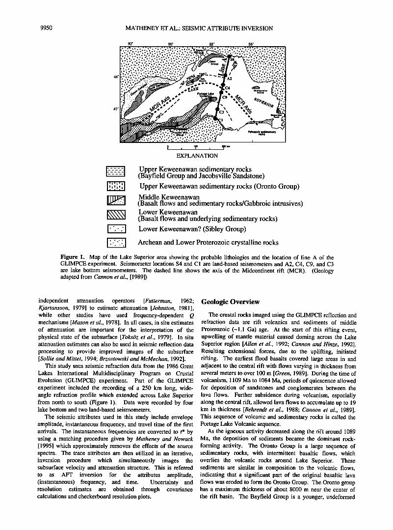
Because of the multiple shot layout of the Lake Superior experiment and the interpolation and smoothing procedure used to process the data, reciprocity of travel times, amplitudes, and t* can be used to check for consistency and accuracy of the data picks. Figure 4 shows plots of seismic attributes versus midpoint for the different record sections. In these plots, reciprocity points fall halfway between receiver locations. This provides a simple graphical check for reciprocity. Reciprocity locations are shown on Figure 4 by vertical dashed lines halfway between the different receiver locations. For the resulting travel times, reciprocity is satisfied given an uncertainty of 0.06 s. This uncertainty is determined interactively during the picking of the first arrival travel times.

Reciprocity plots can also be used to check the amplitude and t* values for consistency. However, while the travel times are absolute values, the amplitudes and t* values are normalized to the reference pulse distance. Therefore any differences in amplitude or t* between the shot location and the reference pulse (in this case a source-reference distance of 1.76 km) would not be accounted for in the reciprocity plot. Considering that the four central shot gathers are all lake bottom instruments and that the source is close to the reference

pulse, the reciprocity plots will still be useful for checking consistency and accuracy in the data picks in this experiment. Figure 4b shows the In-amplitude with midpoint. The vertical dashed lines show the reciprocity locations. Reciprocity is still approximately satisfied within the _+0.5 data uncertainties in the In-amplitudes. Figure 4c shows t* versus midpoint. Reciprocity is also approximately satisfied given a t*

MATHENEY ET AL.: SEISMIC ATTRIBUTE INVERSION 9953

4

LAKE SUPERIOR MID-POINT -VS- TIME GATHER

a)

50 100 150 200 250

•/•d-point (kin)

-lO

MID-POINT VS AMPLITUDE

i i i . , .

50 100 150 200 250

Mk-point

0.06

0.04

0.02

0.00

c)

MID-POINT VS T* i .... i i !

ß , i .... i i i i . .

50 100 150 200 250

Mk-point (km)

Figure 4. (a) Travel times plotted with the midpoint between sources and receivers to better show reciprocity. Dashed, vertical lines are the reciprocity locations between gathers. (b) Amplitudes with midpoint. (c) t* with midpoint. Note that reciprocity is matched at all locations for each attribute within data uncertainties.

uncertainty of _+0.004 s. Both the amplitude and t* uncertainties are obtained by estimating the magnitude of the scatter about the interpolated and smoothed data points shown in Figures 3b and 3c. Record sections S4 and C1 are not included in the reciprocity plots for amplitude and t* because of the larger source-receiver offset of the reference pulse.

Inversion Method

We present a brief description of the inversion method. A more detailed account is given by Nowack and Matheney [1997]. Owing to curved rays associated with seismic

refraction data, a simultaneous inversion of the seismic

attributes is used. Separate inversions of amplitude and t* would need to account for the velocity component in these parameters. The model parameters, slowness and Q-l, are specified at node locations with a spline interpolation of both parameters. The model parameters are related to the seismic attributes through the linearized relation

• * -- I i•t lieu i•t* / i•Q -l ln A L•l ln A l i}u •} ln A l i}Q -•

(3)

9954 MATHENEY ET AL.' SEISMIC ATFRIBUTE INVERSION

where T is the travel time, t* is the attenuation factor, and

ln A is the In-amplitude. The calculated travel times, amplitudes, and t* are obtained by kinematic and dynamic ray- tracing. The amplitudes include geometric spreading and attenuation. The geometric spreading component of the amplitude is computed using dynamic ray methods [Cerven• and Hron, 1980] where the validity of ray methods requires a smoothly varying medium [Ben-Menahern and Beydoun, 1985]. The travel time, amplitude and t* partials are obtained from perturbation analysis [Nowack and Lutter, 1988a; Nowack and Lyslo 1989; Nowack and Matheney, 1997].

The solution of (3) is obtained by iterative, damped least squares which at the n 'h iteration solves

d - •'(•n ) = Gn (• - •n ) (4)

where d is the data vector, •('•n) is the solution of the forward problem at the n th iteration, G n is the sensitivity matrix, and .• is the model parameter vector.

Normalization of the data and model residual vectors is

accomplished by weighting the data residuals by the estimated data covariance matrix C d and the model residuals by a weighting matrix Cx,. The data covariance matrix C a is assumed to be diagonal with the diagonal elements given by the squared data uncertainties. The diagonal components of the

model weighting matrix Cx, are proportional to prior estimates of the squared model errors and inversely proportional to the block size of the parameterization of the model. The variable block weighting removes the effects of unequal block sizes in the discretization of the model [Nolet, 1987]. The prior errors of the model parameters used are 0.15 km/s for the velocity and 0.0020 for Q". These weights

result in the vectors •' = C• 112 (t• - •('•n )) and .•, _-1/2 = Cx n (•n+l - Xn) ß The solution of the linearized problem

is then

,T , -1 , -' .•': (G n G n +I) Gnd' (5)

4.00 -

3.00 _

2.00 - 1.00 -

0.00

North

REDUCED TIMES (STARTING MODEL) 5.00 -

- + observed

- - calculated

, I , I

!0o, Distance (km) 200, RMS error= 0.775 Data error= 0.060

NORMALIZED AMPLITUDES

0.00 -

•ø-2 O0 '•-4 .oo -

-6.00 -

-8.oo - b)

North

, I , I ,

100. 200, RMS error=2.334 Distance (kin) Data error= 0.500

t*

0.04

0.03

0.02 0.01

0.00

100, 200, RMS error= 0.006 North Distance (km) Data error= 0.004

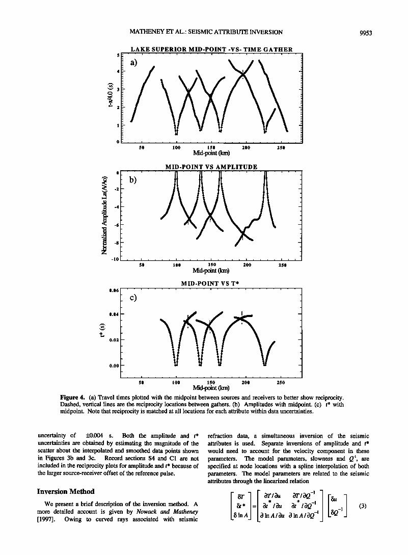
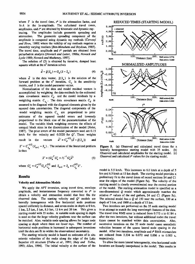
Figure 5, (a) Observed and calculated travel times for a laterally homogeneous starting model with 35 nodes. (b) Observed and calculated amplitudes for the starting model. (c) Observed and calculated t* values for the starting model.

_ _1/2.•, , _-1/2_ _1/2 and Xn+ 1 --'•n 4-C'xn . where G n =c d CinCxn

Results

Velocity and Attenuation Models

We apply the AFT inversion, using travel time, envelope amplitude, and instantaneous frequency converted to t* to obtain a velocity and attenuation model that best fits the observed data. The starting velocity and Q" models are laterally homogenous with five horizontal node positions spaced uniformly in distance, and seven nodes in depth at 0 km, 1 km, 2.5 km, 5 km, 8.5 km, 13 km and 20 km. This gives a starting model with 35 nodes. A variable node spacing in depth is used so that the large velocity gradients near the surface can be matched. Also, variable node spacing allows for larger node spacing at depth where there are fewer rays. The number of horizontal node positions is increased in subsequent inversions until the data are fit to within the observational uncertainty.

The starting velocity model is based on estimates of in situ seismic velocities of the rocks along the edge of the Lake Superior rift structure [Trdhu et al., 1991; Shay and Trdhu, 1993; Allen, 1994]. The initial velocity at the surface of the

model is 5.5 km/s. This increases to 6.0 km/s at a depth of 5 km and 6.5 km/s at 13 km depth. The starting model provides a preliminary fit to the travel times of record sections S4 and C1 near the edges of the model (Figure 5a). The velocity of the starting model is clearly overestimated near the central portion of the model. The starting attenuation model is specified as a one-dimensional Q model which approximately matches the relative t* values of the end gathers, S4 and C1 (Figure 5c). The selected model has a Q of 150 near the surface, 330 at a depth of 5 km, and 1000 at a depth of 13 km.

Two iterations are performed on the 35 node starting model in an attempt to match the long wavelength features of the data. The travel time RMS error is reduced from 0.775 s to 0.184 s after the two iterations, but without additional nodes the travel times cannot be matched within data uncertainties. Also, successive iterations on the 35 node model cause unrealistic

velocities because of the sparse lateral node spacing in the model. After two iterations, amplitude and t* RMS mismatches are reduced from 2.334 to 0.672 and 0.006 s to 0.003 s, respectively.

To allow for more lateral heterogeneity, nine horizontal node locations are linearly interpolated in the model. This results in

MATHENEY ET AL.: SEISMIC ATTRIBUTE INVERSION 9955

REDUCED TIMES (119 NODE MODEL)

A

5.00 •- + observed ' - calcul

4.00 - .

3. O0 .

2.00 -

1 .oo - .

- a) I

100. Distance (km) 200' RMS erro:: 0.052 Data error= 0.060

NORMALIZED AMPLITUDES

0.00

North

• 0.00

•.• -2.00 _• -4.00

• -6. O0 • -8. O0

200. RMS error= 0.347 North Distance (kin) Data error= 0.500

100.

.

A

0.04 -

0.03 -

0.02 -

0.01

0.00

i

North

m I I I •

100 'Distance (km) 200. RMS error= 0.002 Data error= 0.004

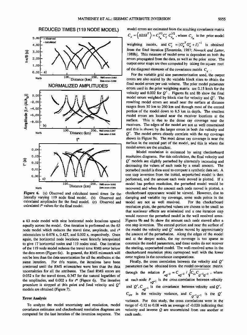
Figure 6. (a) Observed and calculated travel times for the laterally varying 119 node final model. (b) Observed and calculated amplitudes for the final model. (c) Observed and calculated t* values for the final model.

a 63 node model with nine horizontal node locations spaced equally across the model. One iteration is performed on the 63 node model which reduces the travel time, amplitude, and t* mismatches to 0.078 s, 0.427, and 0.002 s, respectively. Once again, the horizontal node locations were linearly interpolated to give 17 horizontal nodes and 119 nodes total. One iteration of the 119 node model reduces the travel time RMS error below

the data errors (Figure 6a). In general, the RMS mismatch will not be less than the data uncertainties for all the attributes at the

same iteration. For this reason, the iterations have been continued until the RMS mismatches were less than the data

uncertainties for all the attributes. The final RMS errors are

0.052 s for the travel times, 0.347 for the natural logarithm of the amplitudes, and 0.002 s for t* (Figure 6). The iterative procedure is stopped at this point and final velocity and Q-1 models are obtained (Figure 7).

Error Analysis

To analyze the model uncertainty and resolution, model covariance estimates and checkerboard resolution diagrams are computed for the last iteration of the inversion sequence. The

model errors are estimated from the resulting covariance matrix

= Cxn C x CXn , where Cxn is the prior model , .G,T -1 weighting matrix, and C x =( n G• +I) is obtained

from the final iteration [Tarantola, 1987; Nowack and Lutter, 1988b]. This measure of model error is dependent on both the errors propagated from the data, as well as the prior error. The output error maps are then computed by taking the square root

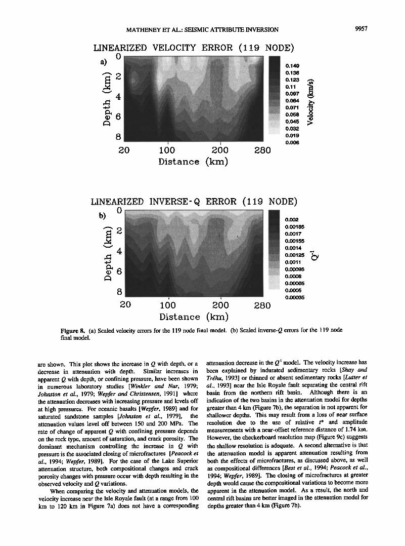
of the diagonal elements of the covariance matrix C x . For the variable grid size parameterization used, the output

errors are also scaled by the variable block sizes to obtain the final model errors per unit volume. The prior model parameter errors used in the prior weighting matrix are 0.15 km/s for the velocity and 0.002 for Q-i . Figures 8a and 8b show the final model errors weighted by block size for velocity and Q-l. The resulting model errors are small near the surface at distance ranges from 50 km to 260 km and through most of the central portion of the model down to 8.5 km in depth. The smallest model errors are located near the receiver locations at the

surface. This is due to the dense ray coverage near the receivers. The edges of the model are not as well constrained and this is shown by the larger errors in both the velocity and Q-l. The model errors closely correlate with the ray coverage shown in Figure 9a. The most dense ray coverage is near the surface in the central part of the model, and this is where the model errors are the smallest.

Model resolution is estimated by using checkerboard resolution diagrams. For this calculation, the final velocity and Q-i models are slightly perturbed by alternately increasing and decreasing the values of each node by a small amount. The perturbed model is then used to compute a synthetic data set. A one step inversion from the initial, unperturbed model is then performed, and the amount each node moved is plotted. If a model has perfect resolution, the perturbed model would be recovered and when the amount each node moved is plotted, a checkerboard appearance would be viewed. However, due to damping and variable ray coverage, some node points in the model are not as well resolved. For the checkerboard

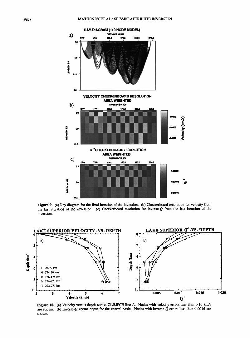
resolution plots, the perturbed values are chosen to be small so that nonlinear effects are minimized and a one iteration step would recover the perturbed model in the well resolved areas. Figures 9b and 9c show the amount each node moved after a one step inversion. The central portion and near the surface of the model the velocity and Q-i nodes moved by approximately the amount of the perturbation. Along the edges of the model and at the deeper nodes, the ray coverage is too sparse to constrain the model parameters, and these nodes do not recover the starting, unperturbed model. The well-resolved areas in the checkerboard resolution plots correspond well with the lower error regions in the covariance computations.

Finally, the cross correlation between the velocity and parameters can be obtained from the model covariance matrix

= • where through the relation PvQ_ 1 CvQ_ 1 / CvvCQ_iQ_i, at each node PvQ_ 1 is the cross correlation between velocity and Q-l, CvQ_ 1 is the covariance between velocity and Cvv is the velocity variance, and is the CQ-IQ-1 variance. For this study, the cross correlations were in the range of-0.12 to 0.08 with an average of-0.020 indicating that velocity and inverse Q are uncorrelated from one another at each node.

9956 MATHENEY ET AL.: SEISMIC ATrRIBUTE INVERSION

a)

b)

VELOCITY MODEL (110 NODE)

4.4 •:•

4.8 '• 5.6 ;> 6 6.4

lO 20 lOO 200 280

Distance (krn)

INVERSE-Q MODEL (119 NODE) $4 A2 CA C9 C3 Cl v v v v v v

100 200 Disanc e (km)

4

0.0165

0,015

•'"'"'•'"'•• 0.0135 i!•!'-.' :•I:?: 0-012

!'?• 0,0075 0,006

•- 0,0045

0,003

0.0015

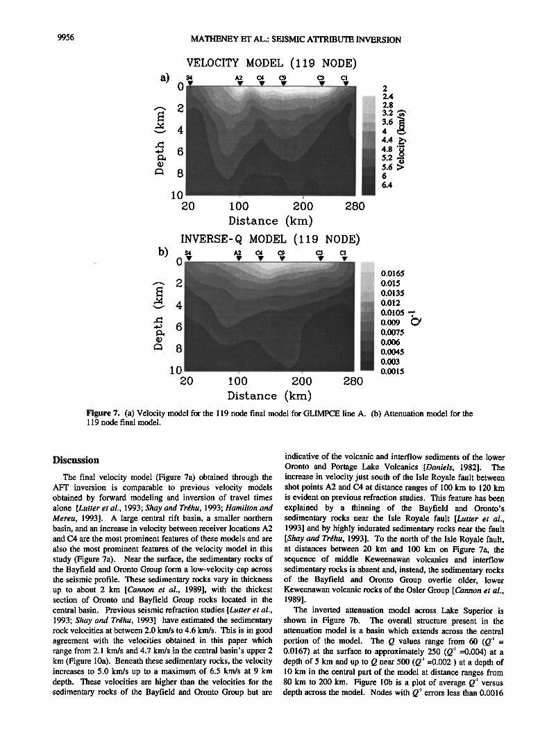
Figure 7. (a) Velocity model for the 119 node final model for GLIMPCE line A. (b) Attenuation model for the 119 node final model.

Discussion

The final velocity model (Figure 7a) obtained through the AFT inversion is comparable to previous velocity models obtained by forward modeling and inversion of travel times alone [Lutter et al., 1993; Shay and Trdhu, 1993; Hamilton and Mereu, 1993]. A large central rift basin, a smaller northern basin, and an increase in velocity between receiver locations A2 and C4 are the most prominent features of these models and are also the most prominent features of the velocity model in this study (Figure 7a). Near the surface, the sedimentary rocks of the Bayfield and Oronto Group form a low-velocity cap across the seismic profile. These sedimentary rocks vary in thickness up to about 2 km [Cannon et al., 1989], with the thickest section of Oronto and Bayfield Group rocks located in the central basin. Previous seismic refraction studies [Lutter et al., 1993; Shay and Trdhu, 1993] have estimated the sedimentary rock velocities at between 2.0 km/s to 4.6 km/s. This is in good agreement with the velocities obtained in this paper which range from 2.1 km/s and 4.7 km/s in the central basin's upper 2 km (Figure 10a). Beneath these sedimentary rocks, the velocity increases to 5.0 km/s up to a maximum of 6.5 km/s at 9 km depth. These velocities are higher than the velocities for the sedimentary rocks of the Bayfield and Oronto Group but are

indicative of the volcanic and interflow sediments of the lower Oronto and Portage Lake Volcanics [Daniels, 1982]. The increase in velocity just south of the Isle Royale fault between shot points A2 and C4 at distance ranges of 100 km to 120 km is evident on previous refraction studies. This feature has been explained by a thinning of the Bayfield and Oronto's sedimentary rocks near the Isle Royale fault [Lutter et al., 1993] and by highly indurated sedimentary rocks near the fault [Shay and Trdhu, 1993]. To the north of the Isle Royale fault, at distances between 20 km and 100 km on Figure 7a, the sequence of middle Keweenawan volcanics and interflow sedimentary rocks is absent and, instead, the sedimentary rocks of the Bayfield and Oronto Group overlie older, lower Keweenawan volcanic rocks of the Osier Group [Cannon et al., 1989].

The inverted attenuation model across Lake Superior is shown in Figure 7b. The overall structure present in the attenuation model is a basin which extends across the central

portion of the model. The Q values range from 60 (Q" = 0.0167) at the surface to approximately 250 (Q-I -'0.004) at a depth of 5 km and up to Q near 500 (Q-I =0.002 ) at a depth of 10 km in the central part of the model at distance ranges from 80 km to 200 km. Figure 10b is a plot of average Q-I versus depth across the model. Nodes with Q" errors less than 0.0016

MATHENEY ET AL.: SEISMIC ATYRIBUTE INVERSION 9957

LINEARIZED VELOCITY ERROR . ::.---;•.:._ •'•,-.:-•','•:f.•'."• .............. i:!•:i.i! -'. ........... • :.:.:.;.•.•:;•:•.?!.....::;:::?•.

8

(119 NODE)

20 100 200 280

Distance (km)

0.149

0.136

0.123

0.11

0.097

ß ..-• 0.084 :;:

•:• 0.071

'"• 0.058 ': 0.045

0.032

0.019

0.006

LINEARIZED INVERSE-Q ERROR (119 NODE) ; ' .

0.00.185

2 o,oo,, 0.00155

4 " o.oo,, • 0.00'11

(1.) 6 O.(XX)95 0.00065

20 100 200 280

Distance (km) Figure 8. (a) Scaled velocity errors for the 119 node final model. (b) Scaled inverse-Q errors for the 119 node final model.

are shown. This plot shows the increase in Q with depth, or a decrease in attenuation with depth. Similar increases in apparent Q with depth, or confining pressure, have been shown in numerous laboratory studies [Winkler and Nur, 1979; Johnston et al., 1979; Wepfer and Christensen, 1991] where the attenuation decreases with increasing pressure and levels off at high pressures. For oceanic basalts [Wepfer, 1989] and for saturated sandstone samples [Johnston et al., 1979], the attenuation values level off between 150 and 200 MPa. The

rate of change of apparent Q with confining pressure depends on the rock type, amount of saturation, and crack porosity. The dominant mechanism controlling the increase in Q with pressure is the associated closing of microfractures [Peacock et a!., 1994; Wepfer, 1989]. For the case of the Lake Superior attenuation structure, both compositional changes and crack porosity changes with pressure occur with depth resulting in the observed velocity and Q variations.

When comparing the velocity and attenuation models, the velocity increase near the Isle Royale fault (at a range from 100 km to 120 km in Figure 7a) does not have a corresponding

attenuation decrease in the Q'• model. The velocity increase has been explained by indurated sedimentary rocks [Shay and Trdhu, 1993] or thinned or absent sedimentary rocks [Lutter et al., 1993] near the Isle Royale fault separating the central rift basin from the northern rift basin. Although there is an indication of the two basins in the attenuation model for depths greater than 4 km (Figure 7b), the separation is not apparent for shallower depths. This may result from a loss of near surface resolution due to the use of relative t* and amplitude measurements with a near-offset reference distance of 1.74 km.

However, the checkerboard resolution map (Figure 9c) suggests the shallow resolution is adequate. A second alternative is that the attenuation model is apparent attenuation resulting from both the effects of microfractures, as discussed above, as well

as compositional differences [Best eta!., 1994; Peacock et al., 1994; Wepfer, 1989]. The closing of microfractures at greater depth would cause the compositional variations to become more apparent in the attenuation model. As a result, the north and central rift basins are better imaged in the attenuation model for depths greater than 4 km (Figure 7b).

9958 MATHENEY ET AL.: SEISMIC ATFRIBUTE INVERSION

RAY-DIAGRAM (119 NODE MODEL)

20`O 70,0 120,0 170,0 220,0

o.o •!•i. • ..!• .... .' •-.-', . .'"' '.:i:': ' ':.. ' '...!11 i' "•" .'.•

ß .•%.

1o•

b)

VELOCITY CHECKERBOARD RESOLUTION AREA WEIGHTED

DISTANCE IN KM

....

................ •%•-•.•!• '"' •'"'•?:*•"•'"•',/**•?•'•11 ............ • 'i::i• •:•'•:/ '•' •"

.

:

.

.

lO,O

270.0

c)

Q 4CHECKERBOARD RESOLUTION AREA WEIGHTED

DISTAHCE IN KM

20.0 70.0 120•0 170`O 220.0 270.0 :' ....... :::zzY.'". ........ I .. . "'z":.;;• z :.

ß .'":;•;•":;•i I :'::'" : ' ' " ... .. ::.;--..*.'.'.....,...•;': ....... •,:;; . ....... . i;* *; ....................... ::. !::.i•?:': . . ..

.. :

.

.... . ....... .. . . ... ,. .

:,:.!; :

;':':' i :'" ; : ',;•. :. .. :,.. • ;

--.a;......,.%. ::. ... .......... . ..... .:

:-.. .

:.

lo.o

o, oooo

.0.0006

Figure 9. (a) Ray diagram for the final iteration of the inversion. (b) Checkerboard resolution for velocity from the last iteration of the inversion. (c) Checkerboard resolution for inverse-Q from the last iteration of the inversion.

L.&KE SUPERIOR VELOCITY -VS- DEPTH 0

2

8

[] 223-271 km

0

2

10

LAKE SUPERIOR Q]-VS- DEPTH

Velocity (km/s) Q• Figure 10. (a) Velocity versus depth across GLIMPCE line A. Nodes with velocity errors less than 0.10 km/s are shown. (b) Inverse-Q versus depth for the central basin. Nodes with inverse-Q errors less than 0.00!6 are shown.

0.020

MATHENEY ET AL.' SEISMIC ATI'RIBUTE INVERSION 9959

0.018 0.016

0.014 0.012

o.oo o.oo 0.004

0.002

2 2.5 3 3.5 4 4.5 5 5.5 6 6.5

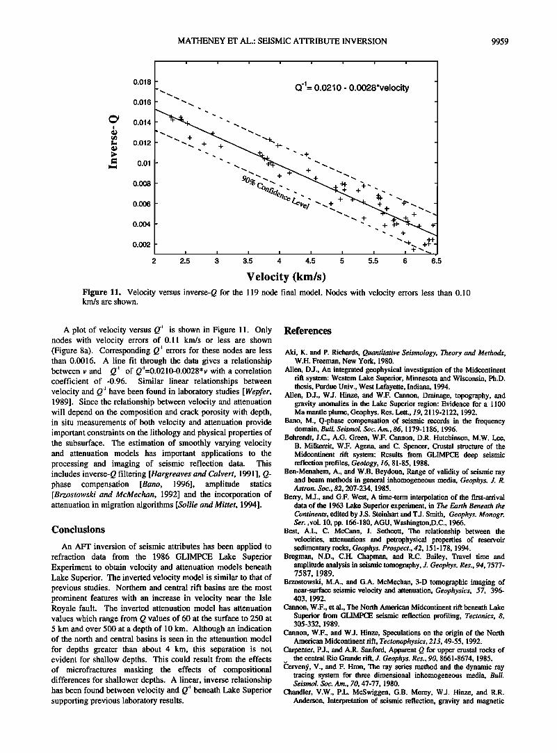
Velocity (km/s) Figure 11. Velocity versus inverse-Q for the 119 node final model. Nodes with velocity errors less than 0.10 km/s are shown.

A plot of velocity versus Q-• is shown in Figure 11. Only nodes with velocity errors of 0.11 km/s or less are shown (Figure 8a). Corresponding Q-• errors for these nodes are less than 0.0016. A line fit through the data gives a relationship between v and Q'• of Q'•=0.0210-0.0028*v with a correlation coefficient of-0.96. Similar linear relationships between velocity and Q-' have been found in laboratory studies [Wepfer, 1989]. Since the relationship between velocity and attenuation will depend on the composition and crack porosity with depth, in situ measurements of both velocity and attenuation provide important constraints on the lithology and physical properties of the subsurface. The estimation of smoothly varying velocity and attenuation models has important applications to the processing and imaging of seismic reflection data. This includes inverse-Q filtering [Hargreaves and Calvert, 1991 ], Q- phase compensation [Bano, 1996], amplitude statics [Brzostowski and McMechan, 1992] and the incorporation of attenuation in migration algorithms [Sollie and Mittet, 1994].

Conclusions

An AFT inversion of seismic attributes has been applied to refraction data from the 1986 GLIMPCE Lake Superior Experiment to obtain velocity and attenuation models beneath Lake Superior. The inverted velocity model is similar to that of previous studies. Northern and central rift basins are the most prominent features with an increase in velocity near the Isle Royale fault. The inverted attenuation model has attenuation values which range from Q values of 60 at the surface to 250 at 5 km and over 500 at a depth of 10 km. Although an indication of the north and central basins is seen in the attenuation model

for depths greater than about 4 km, this separation is not evident for shallow depths. This could result from the effects of microfractures masking the effects of compositional differences for shallower depths. A linear, inverse relationship has been found between velocity and Q-i beneath Lake Superior supporting previous laboratory results.

References

Aki, K. and P. Richards, Quantitative $eismology, Theory and Methods, W.H. Freeman, New York, 1980.

Allen, D.J., An integrated geophysical investigation of the Midcontinent rift system: Western Lake Superior, Minnesota and Wisconsin, Ph.D. thesis, Purdue Univ., West Lafayette, Indiana, 1994.

Allen, D.J., W.J. Hinze, and W.F. Cannon, Drainage, topography, and gravity anomalies in the Lake Superior region: Evidence for a 1100 Ma mantle plume, Geophys. Res. Lett., 19, 2119-2122, 1992.

Bano, M., Q-phase compensation of seismic records in the frequency domain, Bull. $eisrnol. $oc. Am., 86, 1179-1186, 1996.

Behrendt, J.C., A.G. Green, W.F. Cannon, D.R. Hutchinson, M.W. Lee, B. Milkereit, W.F. Agena, and C. Spencer, Crustal structure of the Midcontinent rift system: Results from GLIMPCE deep seismic reflection profiles, Geology, 16, 81-85, 1988.

Ben-Menahem, A., and W.B. Beydoun, Range of validity of seismic ray and beam methods in general inhomogeneous media, Geophys. J. R. Astron. Soc., 82, 207-234, 1985.

Berry, M.J., and G.F. West, A time-term interpolation of the first-arrival data of the 1963 Lake Superior experiment, in The Earth Beneath the Continents, edited by J.S. Steinhart and T.J. Smith, Geophys. Monogr. $er. ,vol. 10, pp. 166-180, AGU, Washington,D.C., 1966.

Best, A.I., C. McCann, J. Sothcott, The relationship between the velocities, attenuations and petrophysical properties of reservoir sedimentar-y rocks, Geophys. Prospect., 42, 151-178, 1994.

Bregman, N.D., C.H. Chapman, and R.C. Bailey, Travel time and amplitude analysis in seismic tomography, J. Geophys. Res., 94, 7577- 7587, 1989.

Brzostowski, M.A., and G.A. McMechan, 3-D tomographic imaging of near-surface seismic velocity and attenuation, Geophysics, 57, 396- 403, 1992.

Cannon, W.F., et al., The Noah American Midcontinent rift beneath Lake Superior from GLIMPCE seismic reflection profiling, Tectonics, 8, 305-332, 1989.

Cannon, W.F., and W.J. Hinze, Speculations on the origin of the Noah American Midcontinent rift, Tectonophysics, 213, 49-55, 1992.

Carpenter, P.J., and A.R. Sanford, Apparent Q for upper crustal rocks of the central Rio Grande rift, J. Geophys. Res., 90, 8661-8674, 1985.

Cerven9, V., and F. Hron, The ray series method and the dynamic ray tracing system for three dimensional inhomogeneous media, Bull. $eismol. $oc. Am., 70, 47-77, 1980.

Chandler, V.W., P.L. McSwiggen, G.B. Morey, W.J. Hinze, and R.R. Anderson, Interpretation of seismic reflection, gravity and magnetic

9960 MATHENEY ET AL.: SEISMIC ATYRIBU'I• INVERSION

data across middle Proterozoic Mid-continent system, northwestern Wisconsin, eastern Minnesota and central Iowa, AAPG Bull., 73, 261- 275, 1989.

Cline, A., Scalar- and planar-valued curve fitting using splines under tension, Camm. ACM, 17, 218-223, 1974.

Daniels, P.A., Upper Precambrian sedimentary rocks: Oronto Group, Michigan-Wisconsin, in Geology and Tectonics of the Lake Superior basin, edited by R.J. Wold and W.J. Hinze, Mere. Geol. Soc. of Am., 156, 107-134• 1982.

Dickas, A.B., Midcontinent rift system: Precambrian hydrocarbon target, Oil Gas J., 82, 151-159, 1984.

Futterman, W.I., Dispersive body waves, J. Geophys. Res., 67, 5257- 5291, 1962.

Goldberg, D., and C.S. Yin, Attenuation of P-waves in oceanic crust: Multiple scattering from observed heterogeneities, Geophys. Res. Lett.,21, 2311-2314, 1994.

Green, J.C., Physical volcanology of mid-Proterozoic plateau lavas; the Keweenawan North Shore volcanic group, Minnesota, Geol. Soc. Am. Bull., 101,486-500, 1989.

Halls, H.C., Crustal thickness in the Lake Superior region, in Geology and Tectonics of the Lake Superior Basin, edited by R.J. Wold and W.J. Hinze, Mere. Geol. Soc. Am., 156, 239-243, 1982.

Halls, H.C., and G.F. West, A seismic refraction survey in Lake Superior, Can. J. Earth Sci., 8, 610-630, 1971.

Hamilton, D.A., and R.F. Mereu, 2-D tomographic imaging across the North American Midcontinent rift system, Geophys. J. Int., 112, 344- 358, 1993.

Hargreaves, N.D., and A.J. Calvert, Inverse Q filtering by Fourier transform, Geophysics, 56, 519-527, 1991.

Hinze, W.J., N.W. O'Hara, J.W. Trow, and G.B. Secor, Aeromagnetic studies of eastern Lake Superior, in the Earth beneath the continents, edited by J.S. Steinhart and T.J. Smith, Geophys. Monogr. Ser., vol. I0, pp. 95-110, AGU, Washington, 1966.

Hinze, W.J., R.L. Kellogg, and N.W. O'Hara, Geophysical studies of basement geology of the southern peninsula of Michigan, AAPG Bull., 59, 1562-1584, 1975.

Johnston, D.H., Attenuation: A state of the art summary, in Seismic Wave Attenuation, D.H. Johnston, and M.N. Toks/3z, SEG Geophys. Reprint ser. no. 2, pp. 123-135, Tulsa, Oklahoma, Soc. of Explor. Geophys., 1981.

Johnston, D.H., M.N. Toks/3z, and A. Timur, Attenuation of seismic waves in dry and saturated rocks: II. Mechanisms, Geophysics, 44, 691-711, 1979.

Kjartansson, E., Constant Q-wave propagation and attenuation, J. Geophys. Res., 84, 4737-4748, 1979.

LaBerge, G.L., Geology of the Lake Superior Region, Geoscience Press, Phoenix, Arizona, 1994.

Lutter, W.J., A.M. Tr6hu, and R.L. Nowack, Application of 2-D travel- time inversion of seismic refraction data to the mid-continent rift

beneath Lake Superior, Geophys. Res. Lett., 20, 615-618, 1993. Mariano, J., and W.J. Hinze, Gravity and magnetic models of the

Midcontinent rift in eastern Lake Superior, Can. J. Earth Sci., 31, 661- 674, 1994.

Mason, W.P., K.J. Marfurt, D.N. Beshers, and J.T. Kuo, Internal friction in rocks, J. Acoust. Soc. Am., 63, 1596-1603, 1978.

Matheney, M.P., and R.L. Nowack, Seismic attenuation values obtained from instantaneous frequency matching and spectral ratios, Geophys. J. Int., 123, 1-15, 1995.

Nolet, G., Seismic wave propagation and seismic tomography, in Seismic Tomography, edited by G. Nolet, pp. 1-23, Norwell, Mass., 1987.

Nowack, R.L., and W.J. Lutter, Linearized rays, amplitude and inversion, Pure Appl. Geophys., 128, 401-421, 1988a.

Nowack, R.L., and W.J. Lutter, A note on the calculation of covariance and resolution, Geophys. J. Int., 95, 205-207, 1988b.

Nowack, R.L., and J.A. Lyslo, Frechet derivatives for curved interfaces in the ray approximation, Geophys. J., 97, 497-509,1989.

Nowack, R.L., and M.P. Matheney, Inversion of seismic attributes for velocity and attenuation structure, Geophys. J. Int., in press, 1997.

Peacock, S., C. McCann, J. Sothcott, and T. Astin, Experimental measurements of seismic attenuation in microfractured sedimentary rocks, Geophysics, 59, 1342-1351, 1994.

Shay, J., and A.M. Tr6hu, Crustal structure of the central graben of the Midcontinent rift beneath Lake Superior, Tectonophysics, 225, 301- 335, 1993.

Sollie, R., and R. Mittet, Prestack depth migration; sensitivity to macro absorption model, $EG Annu. Meet. Expanded Tech. Program Abstr., 64, 1422-1425, 1994.

Steinhart, J.S., and T.J. Smith (eds.), The Earth Beneath the Continents, Geophys. Monogr. $er., vol. 10, Washington, D.C., 1966.

Tarantola, A., Inverse Problem Theory, Elsevier, New York, 1987. ToksOz, M.N., D.H. Johnston, and A. Timur, Attenuation of seismic

waves in dry and saturated rocks: I. Laboratory measurements, Geophysics, 44, 681-690, 1979.

Tr6hu, A., et al., Imaging the Midcontinent rift beneath Lake Superior using large aperture seismic data, Geophys. Res. Lett., 18, 625-628, 1991.

Wepfer, W.W., Applications of laboratory velocity and attenuation data to studies of the Earth's crust, Ph.D. thesis, Purdue Univ., West Lafayette, Indiana, 1989.

Wepfer, W.W., and N.I. Christensen, Q structure of the oceanic crust, Mar. Geophys. Res., 13, 227-237, 1991.

Winkler, K., and A. Nur, Pore fluids and seismic attenuation in rocks, Geophys. Res. Lett., 6, 1-4, 1979.

Woolard, G.P., Transcontinental gravitational and magnetic profile of North America and its relation to geologic structure, Geol. Soc. Am. Bull., 54, 747-790, 1943.

Zelt, C.A., and R.B. Smith, Travel time inversion for 2-D crustal velocity structure, Geophys. J. Int., 108, 16-34, 1992.

M. Matheney and R. Nowack, Purdue University Department of Earth & Atmospheric Sciences, 1397 Civil Building, West Lafayette, IN 49707. (e-mail: matheney@geo.purdue.edu; nowack@geo.purdue.edu)

A. Tr6hu, Oregon State University College of Oceanic and Atmospheric Sciences, Corvallis, OR 97331. (e-mail: Tr6hu@oce.orst.edu)

(Received May 17, 1996; revised November 5, 1996; accepted January 31, 1997.)