seismic analysis of structures using ec8 - Γιώργος...
TRANSCRIPT

1
Seismic Analysis of StructuresUsing EC8
• EC8 includes a full methodology and regulations to perform seismic analysis of structures
- Ground investigations necessity
• However several issues should be further detailed in each country from a National Annex text. These issues amongst others contain:
- Seismic zone maps and reference ground accelerations
- Parameters S , TB , TC , TD defining horizontal response spectra
- Values of φ (calculation of ψE,i for buildings – safety factor for variableactions)
- Values of γI (importance factor for buildings)
EC8: Design of structures for earthquake resistance

2
Contents of EC8
Section 1 - General
Scope of EC8 – Assumptions, definitions and symbols
Section 2 – Performance requirements and compliance criteria
Basic performance requirements and compliance criteria applicable to buildings and civil engineering works in seismic regions
Section 3 – Ground conditions and seismic action
Rules for the representation and calculation of seismic actions and for their combination with other actions
Section 4 – Design of buildings
General design rules relevant specifically to buildings
Section 5-9 – Specific rules for design of several types of buildings
Design specifications for concrete, steel, composite concrete-steel, timber and masonry buildings
Section 10 – Base isolation
Fundamental requirements and other relevant aspects of design and safety, related to base isolation

3
Earthquake analysis of structures in EC8
Structural types covered by EC8
• Concrete structures • Steel structures
• Composite steel-concrete structures • Timber structures
• Masonry structures

4
Types of Seismic Analysis in EC8
• Lateral Force method of analysis
3n number of modes
But 1st mode (T1) dominates the response(regularity criteria)
- This type of analysis may be applied to buildings whose response isnot significantly affected by contributions of higher modes of vibration.
- Several regularity criteria must be met
T1
T2
3Tn
1st mode (T1)
Seismic actions from equivalent
Sdof (T1)

5
• Modal Response Spectrum analysis
- This type of analysis can be applied to all buildings (including those that fail the regularity criteria of Lateral Force method)
Types of Seismic Analysis in EC8
- Take into account so many modes that at least 90% of the total mass becomes active in earthquake forces
3n number of modes
Need k modes to reach 90% of activated mass during analysis
T1
T2
3Tn
ModesSeismic actions from equivalent
Sdof
T1
Tk
T1
Tk
+ +
Total Structural Response

6
• Non-Linear methods of analysis
- Non-Linear static (pushover) analysis
Types of Seismic Analysis in EC8
- Non-Linear time-history analysis
Non-Linear methods discussion is out of the scope of this Lesson
Modal Response Spectrum analysis application in concrete buildings will be discussed in detail in the following pages.

7
Modal Response Spectrum analysis in EC8
§3. Seismic actions calculation from Response Spectrum
Regulations (EC8)
§4.2.4. Combination coefficients for variable actions
§4.3. Structural analysis
§4.3.1 Modelling
§4.2. Characteristics of earthquake resistant buildings
§4.3.2 Accidental torsional effects
§4.3.3 Methods of analysis
§4.3.3.3 Modal Response Spectrum analysis
§5 Design concepts and criteria for concrete buildings
8
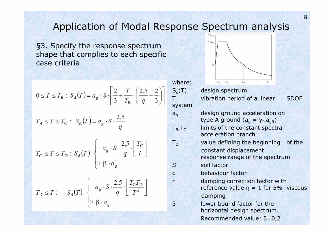
Application of Modal Response Spectrum analysis
§3. Specify the response spectrum shape that complies to each specific case criteria
where:
Sd(T) design spectrum
T vibration period of a linear SDOF system
ag design ground acceleration on type A ground (ag = γI.agR)
TB,TC limits of the constant spectral acceleration branch
TD value defining the beginning of the
constant displacement response range of the spectrum
S soil factor
q behaviour factor
η damping correction factor with reference value η = 1 for 5% viscous
damping
β lower bound factor for the horizontal design spectrum.
Recommended value: β=0,2

9
Application of Modal Response Spectrum analysis
§3.2.4 Inertial effects (mass consideration at each floor)
• Mass calculation of last floor
From load combination G+0.3Q
B G 0.3Qm
g 9.81
• Mass calculation of other floors
From load combination G+0.15Q
B G 0.15Qm
g 9.81
• Accidental torsional effects
In order to cover uncertainties in the location of masses and in the spatial variation of seismic motion the mass location will be displaced from the geometric mass centre (K) by an accidental eccentricity:
ai ie 0.05 L
Li is the floor-dimension perpendicular to the direction of the seismic action
K
Lx
Ly
Ex
Ex
Ey Ey
0.05Ly
0.05Lx

10
Application of Modal Response Spectrum analysis
§3.2.4 Inertial effects (mass consideration at each floor)
K
Lx
Ly
Ex
Ex
0.05Ly
K
Lx
Ly
Ey Ey0.05Lx
K
Lx
Ly
Ex
Ex
Ey Ey
0.05Ly
0.05Lx
Ex
Ey
Ex
Ey
1
2 3
4
mass in 4 different locations (4 different solutions 1,2,3,4)
Design each element with the maximum response values from the
4 solutions

11
Modal Response Spectrum analysis Example 1
Application of Methodology in fixed-base sdof structure
Input data details:
- Concrete structure
- L=4m
- Seismic zone I of Greece
- Agricultural building
- Design for earthquakes with MS>5.5
- Rock soil deposits
- Inverted pendulum system in DCM design
FM
m=5t

12
Modal Response Spectrum analysis Example 1
Earthquake action calculations:
T= 0s
T= TB=0.15s
T= TC=0.4s
T= TD=2.0s
d g
B
2 T 2.5 2 m 2 mS 0 α S 1.26 1.0 0 0.84
3 T q 3 s 3 s
d g
2.5 m 2.5 mS 0.15 α S 1.26 1.0 2.1
q s 1.5 s
d g
2.5 m 2.5 mS 0.4 α S 1.26 1.0 2.1
q s 1.5 s
C
d g
T2.5 m 2.5 0.4 mS 2.0 α S 1.26 1.0 0.42
q T s 1.5 2 s
T= 3.0s C D
d g 2 2
T T2.5 m 2.5 0.4 2 mS 3.0 α S 1.26 1.0 0.19
q T s 1.5 3 s
- Seismic zone I of Greece (agr=0.16g ag=γIagr=0.8·0.16g=1.26m/s²)
- Agricultural building (importance class IV γI=0.8)
- Design for earthquakes with MS>5.5 (Type 1)
- Rock soil deposits (ground type A)
- Inverted pendulum system in DCM design (qo=1.5)
System without walls kw=1
S=1.0 , TB=0.15s , TC=0.4s , TD=2.0s
q=qo·kw= 1.5·1=1.5

13
Modal Response Spectrum analysis Example 1
Mass m=5t
g 2
mβ a 0.2 1.26 0.25
s Lower limit Sd(T)
Response spectrum (5%)
0.00
0.50
1.00
1.50
2.00
2.50
0 0.5 1 1.5 2 2.5 3 3.5 4
T (sec)
Sd
(T)
(m/s
²)T (sec) Sd(T) m/s²
0.00 0.84
0.15 2.10
0.40 2.10
0.50 1.68
0.60 1.40
0.80 1.05
1.00 0.84
1.20 0.70
1.40 0.60
1.60 0.53
1.80 0.47
2.00 0.42
2.20 0.35
2.40 0.29
2.60 0.25
4.00 0.25

14
Modal Response Spectrum analysis Example 1
Modal Response Spectrum Analysis in Sap:
Open File Example 1, select the joint at the top of the structure and assign mass in X-direction equal to 5t.
mass at the top joint Model appearance
15
Modal Response Spectrum analysis Example 1
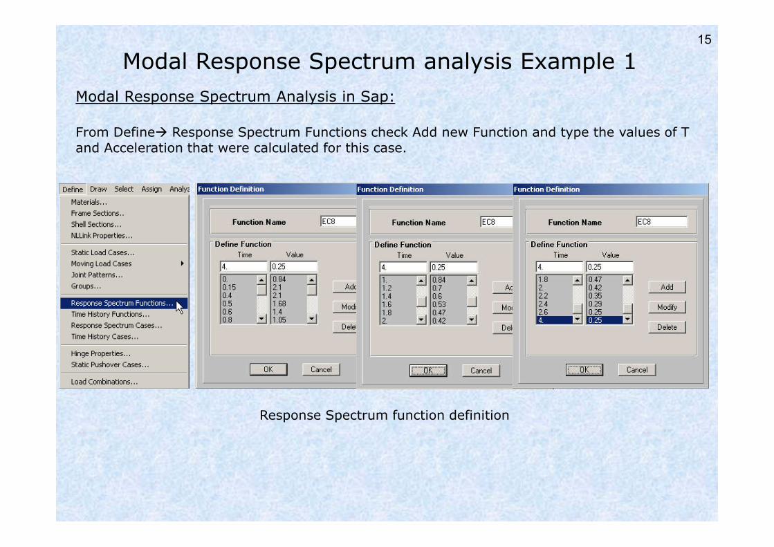
Modal Response Spectrum Analysis in Sap:
From Define Response Spectrum Functions check Add new Function and type the values of T and Acceleration that were calculated for this case.
Response Spectrum function definition

16
Modal Response Spectrum analysis Example 1
Modal Response Spectrum Analysis in Sap:
From Define Response Spectrum Cases check Add new Spectra, select damping 0.05 in modal combination and the EC8 function in Input Response Spectra.
Response Spectrum Case definition
In Analyze Set Options select Dynamic Analysis and from Set Dynamic Parameters ask for 10 modes to be calculated. Since we only have 1 dynamic degree of freedom (1 mass movement in X-direction) we are only expecting from SAP to calculate 1 mode (even when we asked for 10).

17
Modal Response Spectrum analysis Example 1
Modal Response Spectrum Analysis in Sap:
Mode Shape 1 (T=0.3768sec)
Run the analysis. In the right window select Display Show mode shape 1 (mode shape 2 does not exist if we try to ask one).
The period of the structure is T=0.3768. If we look at the calculated response spectrum we can see that the Acceleration value is equal to Sd(0.37)=2.1m/s². Thus the force at the top is F=m·Sd(t)=5·2.1=10.5 KN and the base moment M=10.5KN·4m=42 KNm
From Display Show Elements Forces/Stresses we select Frames and Moment 3-3 diagram in the EC8 Spectra Case.
The diagram shows exactly the same value for the EC8 Spectra case as the calculation by hand.

18
Modal Response Spectrum analysis Example 2
Application of Methodology in 2D plane frame
Input data details:
- Concrete structure
- At each floor g=15KN/m, q=10KN/m
- Bay width 7m
7.0 m7.0 m
Z
Y
XAB
DC
q=10KN/m
g=15KN/m
q=10KN/m
g=15KN/m
g=15KN/m
q=10KN/m
g=15KN/m
q=10KN/m
D
A
3.0
m3.0
m3.0
m3.0
m
- Seismic zone I of Greece
- Ordinary building
- Design for earthquakes with MS>5.5
- Soil deposits of very dense sand with vS,30=450m/s
- Frame system in DCM design

19
Modal Response Spectrum analysis Example 2
Earthquake action calculations:
T= 0s
T= TB=0.15s
T= TC=0.5s
T= TD=2.0s
d g 2 2
B
2 T 2.5 2 m 2 mS 0 α S 1.57 1.2 0 1.26
3 T q 3 s 3 s
d g 2 2
2.5 m 2.5 mS 0.15 α S 1.57 1.2 1.21
q s 3.9 s
d g 2 2
2.5 m 2.5 mS 0.5 α S 1.57 1.2 1.21
q s 3.9 s
C
d g 2 2
T2.5 m 2.5 0.5 mS 2.0 α S 1.57 1.2 0.30
q T s 3.9 2 s
T= 3.0s C D
d g 2 2 2 2
T T2.5 m 2.5 0.5 2 mS 3.0 α S 1.57 1.2 0.13
q T s 3.9 3 s
- Seismic zone I of Greece (agr=0.16g ag=γIagr=0.16g=1.57m/s²)
- Ordinary building (importance class III γI=1)
- Design for earthquakes with MS>5.5 (Type 1)
- Soil deposits of very dense sand with vS,30=450m/s (ground type B)
- Frame system in DCM design (qo=3αu/α1)
Multistorey, multi-bay frame system αu/α1=1.3
Frame system kw=1
S=1.2 , TB=0.15s , TC=0.5s , TD=2.0s
q=qo·kw= (3·1.3)·1=3.9

20
Modal Response Spectrum analysis Example 2
At each floor:
Total G=2·7m·15KN/m=210KN
Total Q=2·7m·10KN/m=140KN
Mass of last floor:
Mass of other floors:
B G 0.3Q 210 0.3 140m 25.69 t
g 9.81 9.81
B G 0.15Q 210 0.15 140m 23.55 t
g 9.81 9.81
Mass calculations from gravity loads
g 2
mβ a 0.2 1.57 0.31
s Lower limit Sd(T)
Response spectrum (5%)
0.00
0.20
0.40
0.60
0.80
1.00
1.20
1.40
0.00 0.50 1.00 1.50 2.00 2.50 3.00 3.50 4.00
T (sec)
Sd
(T)
(m/s
²)
T (sec) Sd(T) (m/s²)
0.00 1.26
0.15 1.21
0.50 1.21
0.60 1.01
0.70 0.86
0.80 0.75
1.00 0.60
1.20 0.50
1.40 0.43
1.60 0.38
1.80 0.34
2.00 0.31
4.00 0.31

21
Modal Response Spectrum analysis Example 2
Modal Response Spectrum Analysis in Sap:
Open File Example 2 and select the joints at the center of the first 3 floors (not the last floor joint) and assign mass in X-direction equal to 23.55t. Repeat the same procedure with the joint at the last floor assigning this time a mass value 25.69t.
mass in 3 first floors mass in last floorModel appearance

22
Modal Response Spectrum analysis Example 2
Modal Response Spectrum Analysis in Sap:
From Define Response Spectrum Functions check Add new Function and type the values of T and Acceleration that were calculated for this case.
Response Spectrum function definition

23
Modal Response Spectrum analysis Example 2
Modal Response Spectrum Analysis in Sap:
From Define Response Spectrum Cases check Add new Spectra, select damping 0.05 in modal combination and the EC8 function in Input Response Spectra.
Response Spectrum Case definition
From Define Load Combinations click Modify/Show on the SEISMIC combo and replace the E Load Case with EC8 Spectra (accurate earthquake loads to replace the simplified).
Replace E load case with EC8 Spectra

24
Modal Response Spectrum analysis Example 2
Modal Response Spectrum Analysis in Sap:
Finally From Define Static Load Cases delete the E Load Case which is now replaced by exact earthquake forces from the spectrum.
Delete E Load Case(simplified earthquake loading)
In Analyze Set Options select Dynamic Analysis and from Set Dynamic Parameters ask for 10 modes to be calculated. Since we only have 4 dynamic degrees of freedom (4 masses movements, one at each floor in X-direction) we are only expecting from SAP to calculate those 4 modes (even when we asked for 10).

25
Modal Response Spectrum analysis Example 2
Modal Response Spectrum Analysis in Sap:
Mode Shape 1 (T=0.425sec)
Run the analysis. In the right window select Display Show mode shape 1 and then Show mode shape 2.
Mode Shape 2 (T=0.136sec)

26
Modal Response Spectrum analysis Example 2
Modal Response Spectrum Analysis in Sap:
In the right window select Display Show elements forces/stresses and Moment 3-3 for the Seismic combo. The moment diagram for this combo is presented. Since the earthquake force does not have a fixed direction, moments at columns can be both positive-negative.
Moment 3-3 diagram

27
Modal Response Spectrum analysis Example 3
Application of Methodology in 3D frame structure
Input data details:
- Concrete structure
- At each floor g=15KN/m, q=10KN/m on beams
- Beam length X-X 6.0m
- Beam length Y-Y 4.0m
- Seismic zone II of Greece
- School
- Design for earthquakes with MS>5.5
- Deep soil deposits of stiff clay with vS,30=300m/s
- Frame system in DCM design

28
Modal Response Spectrum analysis Example 3
Earthquake action calculations:
T= 0s
T= TB=0.20s
T= TC=0.6s
T= TD=2.0s
d g 2 2
B
2 T 2.5 2 m 2 mS 0 α S 2.83 1.15 2.17
3 T q 3 s 3 s
d g 2 2
2.5 m 2.5 mS 0.20 α S 2.83 1.15 2.09
q s 3.9 s
d g 2 2
2.5 m 2.5 mS 0.6 α S 2.83 1.15 2.09
q s 3.9 s
C
d g 2 2
T2.5 m 2.5 0.6 mS 2.0 α S 2.83 1.15 0.63
q T s 3.9 2 s
T= 3.0s C D
d g 2 2 2 2
T T2.5 m 2.5 0.6 2 mS 3.0 α S 2.83 1.15 0.28
q T s 3.9 3 s
- Seismic zone II of Greece (agr=0.24g ag=γI·agr=1.2·0.24g=2.83m/s²)
- School (importance class II γI=1.2)
- Design for earthquakes with MS>5.5 (Type 1)
- Deep soil deposits of stiff clay with vS,30=300m/s (ground type C)
- Frame system in DCM design (qo=3αu/α1)
Multistorey, multi-bay frame system αu/α1=1.3
Frame system kw=1
S=1.15 , TB=0.20s , TC=0.60s , TD=2.0s
q=qo·kw= (3·1.3)·1=3.9

29
Modal Response Spectrum analysis Example 3
At each floor:
Total G=[4·(3·6m)+4·(3·4m)]·15KN/m=1800KN
Total Q=[4·(3·6m)+4·(3·4m)]·10KN/m=1200KN
Mass of last floor:
Mass of other floors:
B G 0.3Q 1800 0.3 1200m 220.18 t
g 9.81 9.81
B G 0.15Q 1800 0.15 1200m 201.83 t
g 9.81 9.81
Mass calculations from gravity loads
Response spectrum (5%)
0.00
0.50
1.00
1.50
2.00
2.50
0.00 0.50 1.00 1.50 2.00 2.50 3.00 3.50 4.00
T (sec)
Sd
(T)
(m/s
²)
g 2
mβ a 0.2 2.83 0.57
s Lower limit Sd(T)
T (sec) Sd(T) m/s²
0.00 2.17
0.20 2.09
0.60 2.09
0.80 1.56
1.00 1.25
1.20 1.04
1.40 0.89
1.60 0.78
1.80 0.70
2.00 0.63
2.10 0.57
4.00 0.57

30
Modal Response Spectrum analysis Example 3
Distributed mass of last floor:
Floor moments of inertia:
2
floor
220.18 tm tμ 1.02
A 12m 18m m
Mass moment of inertia
At each floor, apart from the translational masses there is also a rotational mass degree of freedom around Z-axis. In order to activate this degree of freedom we must calculate the mass moment of inertia:
Distributed mass of other floors:
2
floor
201.83 tm tμ 0.93
A 12m 18m m
3 3
4
x
18m 12 mI 2592 m
12
3 3
4
y
12m 18 mI 5832 m
12
m x yJ μ (I I )
Last floor mass moments of inertia: Other floors mass moments of inertia:
4 2
m 2
tJ 1.02 2592 5832 m 8592.48 tm
m
m x yJ μ (I I )
4 2
m 2
tJ 0.93 2592 5832 m 7834.32 tm
m
X
Y
18
12

31
Modal Response Spectrum analysis Example 3
Modal Response Spectrum Analysis in Sap:
Open File Example 3 and select the joints at the center of the first 3 floors (not the last floor
joint) and assign mass in X and Y directions equal to 201.83t and mass moment of inertia in
Rotation about 3 equal to 7834.32tm². Repeat the same procedure with the joint at the last
floor assigning this time a mass value 220.18t and mass moment of inertia 8592.48tm².
mass in 3 first floors mass in last floor Model appearance
32
Modal Response Spectrum analysis Example 3
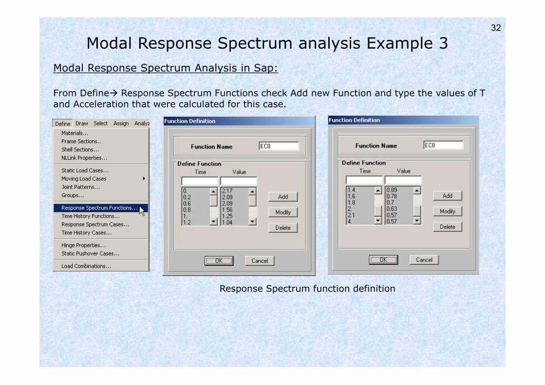
Modal Response Spectrum Analysis in Sap:
From Define Response Spectrum Functions check Add new Function and type the values of T and Acceleration that were calculated for this case.
Response Spectrum function definition

33
Modal Response Spectrum analysis Example 3
Modal Response Spectrum Analysis in Sap:
From Define Response Spectrum Cases check Add new Spectra, select damping 0.05 in modal combination and the EC8 function in Input Response Spectra in direction U1. Repeat the same for EC8Y Case choosing the EC8 function in direction U2.
Response Spectrum Cases EC8-X and EC8-Y

34
Modal Response Spectrum analysis Example 3
Modal Response Spectrum Analysis in Sap:
From Define Load Combinations Delete the EARTHQX and EARTHQY combinations. Then Add two new earthquake Combos as described at the following figures.
Create 2 new earthquake combinations
35
Modal Response Spectrum analysis Example 3
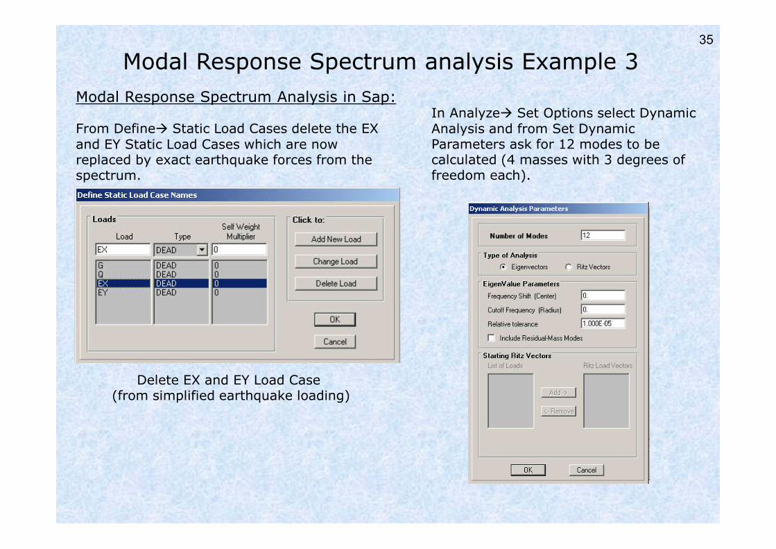
Modal Response Spectrum Analysis in Sap:
From Define Static Load Cases delete the EX and EY Static Load Cases which are now replaced by exact earthquake forces from the spectrum.
Delete EX and EY Load Case(from simplified earthquake loading)
In Analyze Set Options select Dynamic Analysis and from Set Dynamic Parameters ask for 12 modes to be calculated (4 masses with 3 degrees of freedom each).

36
Modal Response Spectrum analysis Example 3
Modal Response Spectrum Analysis in Sap:
Finally the model must be solved in 4 different mass locations as presented in the figure.
Here the solution will take place only for location point 1.
K
Lx
Ex
Ex
Ey Ey
0.05Ly
0.05Lx
Ex
Ey
Ex
Ey
1
2 3
4
mass in 4 different locations (4 different solutions 1,2,3,4)
0.05Lx=0.05·18m=0.9m
0.05Ly=0.05·12m=0.6m
From the right window select the 4 nodes and then from Edit Move enterDelta X=-0.9mDelta Y=0.6m
New appearance with mass at location point 1.
Ly

37
Modal Response Spectrum analysis Example 3
Modal Response Spectrum Analysis in Sap:
Mode Shape 1 (T=0.57sec)
Run the analysis. In the left window select Display Show mode shape 1 and then Show mode shape 2.
Mode Shape 2 (T=0.47sec)
There is some difference from the empirical relationship for 1st mode T=0.1n (n: stories number)This difference is due to the frame system (flexible) without any concrete walls.

38
Modal Response Spectrum analysis Example 3
Modal Response Spectrum Analysis in Sap:
Display moment diagram
In the left window select Display Show elements forces/stresses and then check for Load Case EARTHQX the Moment 3-3.
Column Moment 3-3 for EARTHQX combo

39
Modal Response Spectrum analysis Example 3b
Modal Response Spectrum Analysis in Sap:
If we introduce a few concrete walls at the structure we can study the difference in earthquake response. First File Save As Example 3b. Then create 2 wall frame sections.
Using the XZ view at the right window assign the wall properties at the corner columns of the structure.
WALLXX
WALLXX
WALLYY
XY view XZ view 1 XZ view 2
WALLYY WALLYY WALLXXWALLYYWALLXX
1
2

40
Modal Response Spectrum analysis Example 3b
Modal Response Spectrum Analysis in Sap:
The new appearance of the structure is presented in the figure below. After running the analysis we can view the change in the first mode (T1=0.419sec).
Moreover the function of the concrete walls can be identified by studying the moment developed at their base and compare it with the column moment in the previous model.

41
• Lateral Force method of analysis: application procedure
3n number of modes
But 1st mode (T1) dominates the response (regularity criteria)
- This type of analysis may be applied to buildings whose response isnot significantly affected by contributions of higher modes of vibration.
- Several regularity criteria must be met
T1
T2
3Tn
1st mode (T1)Seismic actions from equivalent
Sdof (T1)
Lateral Force method of analysis
Response spectrum (5%)
0.00
0.50
1.00
1.50
2.00
2.50
0 0.5 1 1.5 2 2.5 3 3.5 4
T (sec)
Sd
(T)
(m/s
²)
T1
SdT1
b T1F Sd m λ
F1
F2
F3
F4
Fn-1
Fn
n
b i1
F F
λ: correction factor
λ=0.85 if Τ1≤2TC , n>2
λ=1 otherwise
Total earthquake force in each direction
Base shear force

42
Lateral Force method of analysis Example 2
Lateral Force method of Analysis in Sap:
7.0 m7.0 m
Z
Y
XAB
DC
q=10KN/m
g=15KN/m
q=10KN/m
g=15KN/m
g=15KN/m
q=10KN/m
g=15KN/m
q=10KN/m
D
A
3.0
m3.0
m3.0
m3.0
m
Input data details:
- Concrete structure
- At each floor g=15KN/m, q=10KN/m
- Bay width 7m
- Seismic zone I of Greece
- Ordinary building
- Design for earthquakes with MS>5.5
- Soil deposits of very dense sand with vS,30=450m/s
- Frame system in DCM design

43
Lateral Force method of analysis Example 2
Earthquake action calculations (Copy from example 2):
T1= 0.4247sec
d g 2 2
2.5 m 2.5 mS 0.4247 α S 1.57 1.2 1.21
q s 3.9 s
ag=γIagr=0.16g=1.57m/s²Importance class III γI=1
Spectrum Type 1
Ground type B: S=1.2 , TB=0.15s , TC=0.5s , TD=2.0s
q=3.9
From modal analysis results (just mass assignment on the structure):
TB < T1 < TC
b 2
mF 1.21 96.34 t 0.85 99.09 KN
s Base shear force:
Total structure mass m=3·23.55+25.69=96.34t (copy from example 2)
i i
i b
j j
z mF F
z m
Horizontal force at each floor:
1
3m 23.55tF 99.09 KN 9.56 KN
732.18 tm
j jz m 23.55t 3m 23.55t 6m 23.55t 9m 25.69t 12m 732.18 tm
2F 19.12 KN
3F 28.68 KN
4F 41.72 KN
iz
im
: height at each floor
: mass of each floor

44
Lateral Force method of analysis Example 2
7.0 m7.0 m
Z
Y
XAB
DC
q=10KN/m
g=15KN/m
q=10KN/m
g=15KN/m
g=15KN/m
q=10KN/m
g=15KN/m
q=10KN/m
D
A
3.0
m3.0
m3.0
m3.0
m
2F 19.12 KN
3F 28.68 KN
4F 41.72 KN
2F 9.56 KN
From File Open Example 2 and Save As Example 2–Lateral Force.
In Define Static Load Cases define a new case named LATERAL
Select the 1st floor joint at the middle column of the structure and assign a horizontal force in X-direction equal to 9.56KN in Load Case “Lateral”.
Repeat the same for all stories applying the respective horizontal loads.

45
Lateral Force method of analysis Example 2
From Define Load Combinations Add 2 combinations named LATSEIS1 and LATSEIS2 (the horizontal force taken in positive and negative direction as an earthquake force) as presented in the figures.
Run the analysis. At the window on the right click Display Show Elements Forces/Stresses and then Moment 3-3 for the LATSEIS1 case (earthquake in the +X direction).
LATSEIS G 0.3Q E

46
Lateral Force method of analysis Example 2
Display also the Moment 3-3 for the LATSEIS2 case (earthquake forces in the –X direction)
Compare the results with the Modal Response Spectrum analysis.
We can see that the results are comparable amongst the two methods of analysis. This similarity depends mainly on the structure regularity, period and type. If the structure’s higher modes play an important role in the response then the two methods of analysis may give results with significant differences.

47
Application of Methodology in 3D frame structure
Input data details:
- Concrete structure
- At each floor g=15KN/m, q=10KN/m
- Beam length X-X 6.0m
- Beam length Y-Y 4.0m
- Seismic zone II of Greece
- School
- Design for earthquakes with MS>5.5
- Deep soil deposits of stiff clay with vS,30=300m/s
- Frame system in DCM design
Lateral Force method of analysis Example 3

48
ag=γI·agr=1.2·0.24g=2.83m/s²)Importance class II γI=1.2)
Ground type C: S=1.15 , TB=0.20s , TC=0.60s , TD=2.0s
Earthquake action calculations (Copy from example 3):
Lateral Force method of analysis Example 3
Spectrum Type 1
q=3.9
From modal analysis results (just mass assignment on the structure) display the structural periods in the two lateral directions. File Open Example 3 and File Display Input/Output Text Files. At the “Modal Participating Mass Ratios” check the period in the two horizontal directions X and Y (large mass ratios).
Y direction T1=0.57sec
X direction T2=0.47sec

49
Lateral Force method of analysis Example 3
T1= 0.5699sec
d g 2 2
2.5 m 2.5 mS 0.5699 α S 2.83 1.15 2.09
q s 3.9 s
TB < T1 < TCY-direction:
T2= 0.4728sec TB < T2 < TCΧ-direction:
d g 2 2
2.5 m 2.5 mS 0.4728 α S 2.83 1.15 2.09
q s 3.9 s
b,X b,Y 2
mF F 2.09 825.67 t 0.85 1466.80 KN
s Base shear force:
Total structure mass m=3·201.83+220.18=825.67t (copy from example 3)
i i
i b
j j
z mF F
z m
Horizontal force at each floor:
1
3m 201.83tF 1466.8 KN 141.53 KN
6275.1 tm
j jz m 201.83t 3m 201.83t 6m 201.83t 9m 220.18t 12m 6275.10 tm
2F 283.06 KN
3F 424.59 KN
4F 617.60 KN

50
Lateral Force method of analysis Example 3
Y-direction:
Χ-direction: Lx
KLy
Ex
0.05Ly
K
Lx
Ly
Ey0.05Lx
0.05Lx=0.05·18m=0.9m
0.05Ly=0.05·12m=0.6m
1F 141.53 KN
2F 283.06 KN
3F 424.59 KN
4F 617.60 KN
1M 0.9m 141.53 KN 127.38 KNm
2M 0.9m 283.06 KN 254.75 KNm
3M 0.9m 424.59 KN 382.13 KNm
4M 0.9m 617.60 KN 555.84 KNm
1F 141.53 KN
2F 283.06 KN
3F 424.59 KN
4F 617.60 KN
1M 0.6m 141.53 KN 84.92 KNm
2M 0.6m 283.06 KN 169.84 KNm
3M 0.6m 424.59 KN 254.75 KNm
4M 0.6m 617.60 KN 370.56 KNm
Mi
Mi
Additional moments to introduce torsional effects:The horizontal forces will be applied at the centre of the plan. The eccentricity will be considered through the additional moment, calculated as follows:

51
Lateral Force method of analysis Example 3
Save as Example 3–Lateral Force having the model with the mass location at the geometrical centre of the floor.From Define Static Load Cases define 2 new Load Cases for the X-direction and Y-direction earthquake forces.
From the 2D view window select successively each joint and apply the horizontal forces and moments that were calculated a each Static Load Case. An example is presented for the joint of the first floor.At each load case the horizontal force and respective moment is assigned at the joint.
Repeat the same procedure for all the stories.

52
Lateral Force method of analysis Example 3
Define Load Combinations and add 4 new combinations as the following figures describe.
X YSEISLAT 1 4 G 0.3Q E 0.3E
X YG 0.3Q E 0.3E
X YG 0.3Q E 0.3E
X YG 0.3Q E 0.3E
X YG 0.3Q E 0.3E
The same procedure must be adopted for the following 4 combinations:
X YSEISLAT 5 8 G 0.3Q 0.3E E

53
Lateral Force method of analysis Example 3
Run the analysis and display the maximum Moment 3-3 from the SEISLAT combinations. Make the comparison with the Modal Response Spectrum method of analysis.
In order to make a full comparison of the results of the two methods we should check all 4 mass locations for the Response Spectrum analysis and all 8 combinations of loads for the Lateral force method.
Lateral Force Analysis (SEISLAT3) Modal Response Spectrum Analysis
(mass Location 1)

54
Review of analysis methods in Eurocode 8
Preliminary Modal Analysis
m1
m2
m3
Results: period T values
STATIC ANALYSIS
DYNAMIC ANALYSIS
From T1 calculate Sd(T1) at each direction (hand calculation)
Calculate base shear force Fb (hand calculation)
Perform Fb distribution with height (hand calculation)
Define static load cases for the earthquake forces
Define appropriate combinations
Perform analysis
Define spectrum Sd shape in computer code
Define Response spectrum cases for the earthquake forces
Define appropriate combinations
Perform analysis

55
Corrections
1) Name the Files as following
- Example 3
- Example 3 - Modes
- Example 3 – Response Spectrum
- Example 3 – Lateral Force
Lateral Force method of analysis Example 3c
- Example 3 – Response Spectrum Location 1