Segmentation and Time-of-Day Patterns inForeign Exchange Markets∗

Angelo Ranaldo†

Swiss National Bank

February 28, 2007

∗The views expressed herein are those of the author and not necessarily those of the SwissNational Bank, which does not accept any responsibility for the contents and opinions ex-pressed in this paper. The author thanks Tim Bollerslev, Alain Chaboud, Thierry Foucault,Albert Menkveld, Marco Pagano, Paolo Pasquariello, Dagfinn Rime, Asani Sarkar, Paul Söder-lind, David Veredas, Paolo Vitale, Katrin Assenmacher and an anonymous referee for theircomments. I am especially grateful to Adrian Trapletti for his insightful suggestions andsupport. All errors remain mine.

†Angelo Ranaldo, Swiss National Bank, Research, Börsenstrasse 15, P.O. Box 2800,Zurich, Switzerland. E-mail: angelo.ranaldo@snb.ch, Phone: ++41.44.6313826, Fax:++41.44.6313901.

Segmentation and Time-of-Day Patterns inForeign Exchange Markets

Abstract: This paper sheds light on a puzzling pattern in foreign exchange

markets: Domestic currencies appreciate (depreciate) systematically during for-

eign (domestic) working hours. These time-of-day patterns are statistically and

economically highly significant. They pervasively persist across many years,

even after accounting for calendar effects. This phenomenon is difficult to rec-

oncile with the random walk and market efficiency hypothesis. Microstructural

and behavioural explanations suggest that the main raison d’être is a domestic-

currency bias coupled with market segmentation. The prevalence of domestic

(foreign) traders demanding the counterpart currency during domestic (foreign)

working hours implies a cyclical net positive (negative) imbalance in dealers’

inventory. In aggregate, this turns into sell-price (buy-price) pressure on the

domestic currency during domestic (foreign) working hours.

Keywords: foreign exchange market; microstructure; behavioural finance; time-

of-day patterns; market segmentation; calendar effects; inventory; asymmetric

information; high-frequency data.

JEL Classifications: F31; G10; G14; G15.

1 Introduction

This paper provides striking evidence on spot exchange rates: Home currencies

depreciate systematically during domestic working hours and appreciate during

the working hours of the foreign counterpart country. Our database covers

more than a decade’s worth of data stored in a high-frequency database, with

several currency pairs that, taken together, cover more than 64% of total market

turnover by currency pair in 2004 (BIS (2005)). A clear picture emerges: first,

this pervasive time-of-day pattern is highly significant, both statistically and

economically; second, it spans many years and overrides calendar effects.

The fact that exchange rates follow cyclical patterns during the day chal-

lenges the random walk and efficient market hypothesis. An efficient market is

one where the market price is an unbiased estimate of the true asset value. De-

viations between true and market prices should be random, not systematic and

cyclical. Given its characteristics, the foreign exchange market is the foremost

aspirant to market efficiency. It is the world’s largest financial market1, with

low transaction costs, and is widely backed by derivative instruments. It is a

real global market open 24 hours a day. In it, various atomistic and price-taking

market participants trade identical assets virtually, from many locations, and

they can react almost instantaneously to news items. Operationally, trades are

triggered on several competing microstructures and exchange systems, such as

through dealers, brokers, ECNs, phone networks and nonbank internet sites.2

Why do so many rational and utility-maximising traders initiating the purchase

of domestic (foreign) currency during domestic (foreign) working hours system-

atically incur recurrent adverse transaction prices? Why do they not arbitrage

this market anomaly in such a competitive environment?

After having documented the statistical and economic significance of this

phenomenon, we attempt to explain why it exists. Two main explanations

emerge: liquidity and asymmetric information effects. The former refers to im-

balances in the inventories of liquidity suppliers that are caused by systematic

excess demand or supply at specific intraday times. The latter refers to the

possibility that traders may profit from superior information because of their

networking, trading location and the time zone in which they operate. We argue

that the former factor is more important. In particular, this main explanation

is derived from a combination of two factors: first, the prevalence of domestic

currencies in the portfolio allocations of domestic investors and second, mar-

1The average daily turnover on the foreign exchange market amounted to $1.9 trillion inApril 2001 (BIS, 2005), more than 5 times the yearly turnover of all equities traded at NYSE.

2E.g. Deal4Free of CMC established in 1996; IFX Markets (since 1999); MatchbookFX(started in 1999 and closed down in 2000); HotSpotFX (since 2001) and Oanda (since 2001).

1

ket segmentation. With respect to these two factors, we will henceforth refer

to ’domestic-currency bias’ and ’domestic-time bias’. The domestic-currency

bias means that traders located in one specific country tend to hold assets de-

nominated in the reference currency of that country. Their portfolios typically

include domestic assets and, therefore, the domestic currency prevails over for-

eign currencies. This idea parallels the international home-bias literature (see

Lewis (1999) for a survey). The domestic-time bias refers to the actual time

when trading is done. Evidence on the imperfect integration of foreign exchange

markets is provided by Hsieh and Kleidon (1996). As in the case of the prox-

imity bias for equity markets (e.g. Massa and Simonov (2006)), we argue that

investors have a tendency to trade mainly in their country’s working hours. For

instance, US investors, brokers and dealers will tend to exchange US dollars

against euros during the main US hours of work. Conversely, the execution of

euro-dollar spot exchanges initiated by European investors is clustered within

the main working hours of central Europe. In a trading environment with an

imperfectly elastic supply, the combination of these two factors gives rise to a

cyclical pattern: the home currency depreciates during domestic working hours

and appreciates during foreign working hours. In aggregate, the geographic

segmentation, coupled with the domestic-currency bias, creates sell-price (buy-

price) pressure on the domestic currency during domestic (counterpart) working

hours.

In order to obtain empirical support for these arguments, we use two meth-

ods to examine currency movements. First, we perform a time-series analysis

of intraday currency returns to examine linkages across time and world regions.

The prevalence of reversal rather than persistent patterns in currency returns

suggests that the liquidity hypothesis is more plausible. Second, a natural ex-

periment is to test what happens when one of the two counterpart countries

or regions is on holiday. If the foreign country is on holiday while people in

the home country are working, it seems likely that during domestic working

hours the domestic sell-pressure on the domestic currency will be exacerbated

by the diminished buy-pressure from foreign investors. On the other hand, dur-

ing foreign working hours, foreign investors will be relatively inactive and will

not exert the usual buy-pressure on the domestic currency. This will result

in stronger depreciation of the home currency during domestic working hours

and weaker appreciation during foreign working hours. Our empirical findings

largely support this supposition.

Surprisingly, the literature to date has almost nothing to say about the

intraday patterns of exchange rate returns. Most of the attention in previous

2

studies has been devoted to intraday volatility or bid-ask spreads, rather than

returns. The Olsen & Associates study was a real pioneer in collecting and

analysing high-frequency data (e.g. Dacorogna et al. (1993), Olsen et al. (1997),

and Müller et al. (1990)). However, its focus was on return volatility, bid-

ask spread size and intensity of market activity, especially for foreign exchange

markets. This is also the case for many other studies that have made significant

contributions to the literature (Andersen and Bollerslev (1997, 1998), Baillie and

Bollerslev (1990), Bollerslev and Domowitz (1993), Hsieh and Kleidon (1996),

and Ito and Hashimoto (2005), just to mention a few). Ito (1987) and Ito and

Roley (1987, 1991) represent an exception. However, they use only five points of

time to analyse the intraday return behaviour of yen-dollar exchange rate from

1980 to 1986. Our study adds to this literature by examining in finer detail the

cross-sectional and time-series characteristics of intraday returns across different

time zones, working time periods and calendar events.

This paper is structured as follows. Section 1 provides statistical evidence on

time-of-day market patterns. Section 2 covers their economic significance. Sec-

tion 3 presents a simple microstructure framework for studying the main drivers

of this phenomenon. Section 4 presents some empirical findings supporting our

hypotheses. Section 5 concludes the paper.

2 Time-of-day patterns

2.1 Data

The database has been kindly provided by Swiss-Systematic Asset Management

SA, Zurich. It includes spot exchange rates for the following currency pairs:

CHF/USD, DEM/USD, EUR/USD, GBP/USD, JPY/EUR and JPY/USD. The

sample periods cover the period from the beginning of January 1993 to the end

of August 2005 for the CHF/USD, GBP/USD and JPY/USD exchange rates,

and from January 1999 to August 2005 for EUR/USD and JPY/EUR. Data

for DEM/USD cover the period from January 1993 to December 1998. The

introduction of the euro dictates the time periods for the euro and the German

mark. We use the tick-by-tick FXFX Reuters midquote price (the average price

between the representative ask and bid quotes). The characteristics of these

data have been discussed at length in previous studies (among others, Müller

et al. (1990), Dacorogna et al. (1993) and Goodhart, Ito and Payne (1996)).

Although indicative quotes have their shortcomings, a comparison of the elec-

tronic foreign exchange trading system, Reuters 2000-2, with FXFX Reuters

shows that "FXFX indicative quotes can be taken as a very good and close

3

proxy for that in the Reuters 2000-2" (Goodhart, Ito and Payne (1996), page

126).3

The dataset contains millions of representative quotes. To conduct this

study, we carefully organised our database as follows: first, we accounted for

changes in daylight savings times, expressing time in terms of Greenwich Mean

Time (GMT). Second, we organised our database in 5-minute intervals. For each

interval, we identified the first, last, high and low exchange rates. If no trades

occurred in a given 5-minute interval, we copied down the last trading price in

the previous time interval. Finally, since our database included weekends, we

excluded weekend hours according to the definitions reported in Table 1. The

definition of weekend hours matches the beginning and end of working hours in

the different time zones. Thus, for each currency pair, the working week begins

at 6 a.m. in the earliest time zone and ends at 6 p.m. in the latest time zone,

expressed in terms of Greenwich Mean Time. For instance, for JPY/USD, the

working week begins when it is 6 a.m. on Monday in Tokyo (corresponding to

9 p.m. on Sunday, GMT) and ends at 6 p.m. on Friday in New York local time

(11 p.m. on Friday, GMT). It is worth stressing that the inclusion of weekends

leaves the main results unchanged. But it has the disadvantage of blurring some

of the intraday effects.

For the sake of presentation, we investigate exchange rate movements over

4-hour periods. These time brackets allow us to observe overlapping and non-

overlapping intraday periods in the different working hours of each world region.

In particular, trading hours from midnight to 4 a.m., from 8 a.m. to midday

and from 4 — 8 p.m. GMT mirror the main trading activity in Japan, Europe

and the US, respectively. A 4-hour time interval is also a reasonable length of

time for marketable intraday trading. In principle, one could question whether

shorter timeframes than four hours provide a finer identification of short-lived

patterns. But it turns out that shorter timeframes deliver a nosier picture of

the same phenomenon. The descriptive analysis over one-hour time intervals is

available upon request.

2.2 Statistical significance

Figure 1 presents time-of-day return patterns in graphical form. Each graph

shows 24 cross-sectional averages of annualised returns over four hours. Using

3Martens and Kofman (1998) show that futures on DM/$ tend to lead the "quoted" spotmarket for up to 3 minutes. This lead-lag relation does not constitute critical evidence forour study. Lyons (1995) stresses three limitations related to "indicative" quotes: they arenot tradable; they are representative only for the interbank market; during very fast markets,"indicative" quotes may be updated with a short delay.

4

two-sample t-tests, these graphs also show if the acceptance of the null hypoth-

esis of equality in means falls below the p-value of 5% or 1%. In figure 1, black

(grey) bars mean that an average return over a specific 4-hour time period is

different at a 1% (5%) significance level.4 These figures clearly show that all

currencies tend to depreciate during the working hours of their reference coun-

tries and to appreciate during the working hours of their counterpart countries.

More specifically, these figures show:

- CHF/USD: the US dollar appreciates significantly from 5:00 to 13:00 GMT

and the Swiss franc appreciates significantly from midday to 17:00 and

then again from 17:00 to 23:00 GMT.

- DEM/USD: similar to CHF/USD, the US dollar appreciates significantly from

5:00 to 13:00 GMT and the German mark appreciates significantly from

midday to 17:00 GMT.

- EUR/USD: the US dollar appreciates significantly from 8:00 to 12:00 GMT

and the euro appreciates significantly from 16:00 to 22:00 GMT.

- GBP/USD: the US dollar appreciates significantly from 4:00 to 12:00 GMT

and the pound sterling appreciates significantly from 11:00 to 18:00 GMT.

- JPY/EUR: the euro appreciates significantly from 1:00 to 6:00 GMT and the

yen appreciates significantly from 8:00 to 15:00 GMT.

- JPY/USD: the US dollar appreciates significantly during the night (from 22:00

to 4:00 GMT) and the yen appreciates significantly from 12:00 to 16:00

GMT.

The trading influence from world regions other than the two counterparties is

weaker, but still visible. In particular, trading in Japanese trading hours appears

to support the US dollar against the euro and against the sterling (see figure 1C

and 1D, during the night from 21:00 to 2:00 GMT), US trading supports the

euro against the yen (figure 1E, 14:00-22:00 GMT) and during European hours

the dollar depreciates against the yen (figure 1F, 5:00-11:00 GMT).

The dollar depreciation (appreciation) against the yen during US (Japanese)

business hours is the weakest pattern we have found (although it is still signif-

icant). Our results apparently contrast with those obtained by Ito and Roley

4These t-statistics refer to two-tail statistics on the difference between a given 4-hour returnmean over all the other 4-hour returns. Note that we perform the two-sample equal variance(homoscedastic) test. This represents a more severe test than the heteroscedastic hypothesis.In fact, the probability associated with a Student’s t-test for equality in means has an upwardbias and leads to a more likely rejection of the inequality hypothesis.

5

(1987), who found opposing patterns from 1980 to 1986. There are several ex-

planations for this apparent anomaly. First, having only five data points in time,

Ito and Roley use a more rigid and rough definition of intraday periods. Sec-

ond, as pointed out by Ito and Roley (1987), the yen-dollar exchange rates from

1980 to 1986 are characterised by the "over-valued" dollar policy and strong

temporary trends. Froot (1991) also shows that Japanese outflows of foreign di-

rect investment increased dramatically in the eighties, and half of the Japanese

capital outflow was directed towards US.

Table 2 and 3 show more detailed descriptive statistics. Here, six non-

overlapping 4-hour time intervals represent the entire trading day. Means, me-

dians and standard deviations are reported on an annualised basis to ease read-

ing. To annualise, 4-hour returns are multiplied by 260. Tests for inequality

in means and medians (Wilcoxon/Mann-Whitney test) corroborate the previ-

ous results. In line with the previous literature, intraday heteroskedasticity is

clearly observable (F-tests show statistical significance). The max and min and

the statistics on the third and fourth moments suggest that distributions are

reasonably centred, acceptably well-shaped with respect to a Gaussian distri-

bution and moderately affected by outliers.5 Among the descriptive statistics,

we report the relative frequency of positive returns (excluding zero returns).

The sign test shows that the proportion of upward and downward intraday

returns significantly matches with the time-of-day patterns plotted in Figure

1A-F, i.e. there are consistently more domestic currency depreciations (appre-

ciations) during domestic (foreign) working hours. It is also interesting to note

that 4-hour returns outside the main working hours are not serially correlated

across consecutive days.6 For instance, for CHF/USD there is an autoregressive

pattern during Swiss and US working hours only. This is another indication

that clock-time influences trading-time.

There are some institutional aspects that can represent a preliminary ex-

planation for the time-of-day patters. First, it is worth noting that there is a

specific point in time that can be considered to be the end of the trading day

5We checked the correspondence between our intraday outliers, using Datastream dailydata. There is consistent matching. In particular, the max and min 4-hour returns forJPY/USD are concentrated around 8 October 1998. On that day, this exchange rate expe-rienced marked fluctuations. The dollar depreciated strongly around 10:00-12:00 GMT andrecovered around 15:00-18:00 GMT. Datastream data indicate that the daily (log) changeson 7 and 9 October 1998 amounted to -7.7% and -2.3%, respectively. (The original source ofthese data is the Global Treasury Information Services, which fix the closing quote at 13:00GMT).

6See "Q-stat 1" in table 2, showing the Q-statistic for testing the null hypothesis thatthere is no autocorrelation at lag 1, i.e. serial correlation between one day’s intraday returnoccurring in a given 4-hour period and the previous day’s intraday return occurring at thesame time of the day.

6

on spot foreign exchange markets. This is 21:00 GMT, the time when the New

York market closes. An open spot position after 21:00 GMT implies the pay-

ment of an interest rate differential between the long currency and the short

currency over the next working day. Our results show that this point in time

has no particular effect on intraday returns. Only in the case of euro-dollar ex-

change rates we do observe significant movement. Second, as discussed by Lyons

(1995), many banks impose overnight limits on their dealers’ positions. More-

over, most dealers close their day with a zero net position and then they restore

their inventory in the early morning of the trading day to face the oncoming

liquidity demand (Lyons (1998)). Thus, intraday and overnight trading limits

may determine time-of-day patterns. Finally, the common practice in foreign

exchange markets is to hedge only partially the aggregate dealer’s position. On

the other hand, dealers tend to adjust unbalanced inventory levels on a single

currency pair over (short) intraday periods. Lyons (1995) shows that FX dealers

prefer to reduce inventory over given thresholds via outgoing orders or brokered

trades. This practice implies a transmission mechanism of transient inventory

imbalances among dealers. Overall, this reasoning provides us a prima facie

explanation for temporary trends in exchange rates due to inventory problems.

2.3 Calendar effects

We examine how intraday returns are distributed across time and whether our

results may be affected by particular calendar effects. In particular, we check

whether these intraday seasonalities cluster at given points of time. There is

no specific month in the year responsible for this phenomenon (not displayed).

Hence, the year-change or January effect that characterises equity markets does

not appear to hold for currencies. Figure 2 shows that the time-of-day anomaly

is evenly distributed across the years. By taking the US investor (European

investor for JPY/EUR) point of view, figure 2A plots domestic currency appre-

ciation during foreign working hours, year by year, from 1993 to 2005. Figure

2B shows domestic currency depreciation during domestic working hours. Only

in a very few cases do we observe exceptions to the general pattern; in partic-

ular, the US dollar appreciated noticeably against the Swiss franc during US

working hours in 1999 and 2005. However, it is evident that the time-of-day

phenomenon persists over years.

Table 4 reports how the time-of-day patterns are spread across weekdays.

For simplicity, we annualise returns. Some interesting results emerge. As far as

the US dollar is concerned, the time-of-day anomaly exerts the strongest effect

during US working time on Thursdays. In general, the US dollar depreciates

7

5%—7% against European currencies during US working hours, and 4% against

the yen. On Thursdays, the dollar experiences an additional depreciation of 2%—

4%. European currencies, including the Swiss currency, appear more affected by

trading activity on Mondays and Wednesdays. Indeed, the euro, German mark

and Swiss franc have a tendency to loose 3% or more than the usual morning

depreciation on Mondays (8:00-12:00 GMT). The additional appreciation of the

euro during this intraday period increases from 7.8% to 15.7% against the yen.

In turn, the yen seems to be more exposed to an end-of-the-week effect. On Fri-

day morning (local time), the yen looses 13.6% on average against the dollar and

10.5% on average against the euro, as compared to the normal 2.7% and 2.9%,

respectively. There are two main arguments that could help to explain these de-

terministic patterns. On the one hand, the non-trading hours over the weekend

may strengthen time-of-day effects on Mondays and Fridays. The weekend ef-

fect on equity markets has been extensively documented (e.g. French (1980)). A

similar effect may exist on currency markets. On the other hand, the literature

shows that major public information announcements, such as macroeconomic

news, have a significant effect on foreign exchange rates (cf. among others, An-

dersen et al. (2003), Andersen and Bollerslev (1998), Bauwens, Ben Omrane and

Giot (2005), Ederington and Lee (1993), Evans and Lyons (2005)). Since these

news announcements are pre-scheduled and released recurrently on the same

day of the week, the day-of-the-week effect discussed above may be related to

information releases. Finally, an additional issue that may influence intraday

price movements is the occurrence of central bank interventions. However, these

are typically conducted on an irregular and occasional basis. Moreover, the lit-

erature shows that intervention operations are controversial policy options and

may lead to mixed results (e.g. Dominguez (1998)). So, it is hard to believe

that deterministic patterns such those in table 4 can be explained by irregular

events such as central bank interventions.

3 Economic significance

While this time-of-day phenomenon appears highly significant in statistical

terms, a further natural question would be whether it is also significant in eco-

nomic terms. We attempt to answer this question by applying some simple

trading rules. Five main rules are investigated. Their performance is sum-

marised in Table 5. The first (second) rule consists in taking a long (short)

position each working day for four of the foreign (domestic) working hours. The

long position on US dollars is from 8:00 to noon if the counterpart currency

8

is the Swiss franc, German mark, euro or pound sterling, and from midnight

to 4:00 as far as the yen is concerned. The short position on the dollar spans

the hours from midday to 16:00 if the counterpart currency is the Swiss franc,

German mark, pound sterling or Japanese yen, and from 16:00 to 20:00 for the

euro. The short positon on euro against yen occurs from 8:00 to noon. The

third strategy combines the first two rules, i.e. a long-short strategy each day.

Since we have observed some day-of-the-week effects, the fourth and fifth strate-

gies focus only on one specific trading day in the week. The fourth trading rule

implements a short-long strategy on Mondays only. This should have a partic-

ularly positive effect on performance during European working times. The final

trading rule executes a short-long strategy on Thursdays or Fridays only. These

specific days are consistent with the day-of-the-week effects reported in Table

4. Taking annualised values, performance is evaluated in terms of mean return,

standard deviation and Sharpe ratio. We also implement a simple time-series

analysis by estimating a one-factor model as follows:

rSt = α+ βrDt + t (1)

The dependent variable rSt is the intraday return on day t resulting from

the strategy S that could be one of the five trading rules explained above. The

return on the benchmark asset rDt is represented by the daily (log) change on

the currency pair. The day is defined as lasting from 0:00 to 24:00 GMT. Other

definitions provide essentially the same results. In the LS regressions, we apply

the heteroskedasticity consistent covariance matrix estimator as proposed in

White (1980). The factor model estimation gives the size of alpha (annualised)

and beta that can be interpreted in the traditional sense, namely the risk-

adjusted Jensen measure and the beta coefficient as a measure of systematic

risk.

It is worth emphasising that the implementation of these rules does not aim

at maximising profitability. In fact, to be consistent with the rest of the paper,

these rules are applied to the six four-hour periods mentioned above and not

to the intraday periods affording the maximum average returns. For instance,

the long position on Japanese yen taken by a European investor trading on

JPY/EUR has been set for the midnight—4:00 time intervals (GMT) that provide

a return of only 2.8%. This position would earn 7.6% if carried out from 17:00—

22:00. Furthermore, more sophisticated operations such as the use of leverage

or (intraday) timing are simply ignored.

Table 5 shows that even the minimal long and short rules provide signif-

icant results in economic terms. The combined long and short strategy in-

9

creases performance twofold. Long-short strategy performance ranges from 5.9%

(GBP/USD) to 16.7% (EUR/USD). These numbers translate into 0.9 and 2.41

in terms of Sharpe ratios. The implementation of day-of-the-week strategies

magnifies these yields further. The long-short strategy on Mondays and Thurs-

days attains almost 20% of annual returns, with a Sharpe ratio of more than

3.5.

The factor model estimation for equation (1) yields the following results.

First, alphas are exactly in line with the mean returns reported above. Sec-

ond, beta estimates suggest a fairly low exposure to systematic risk. Betas (in

absolute values) for long and short trading rules (taken separately) are around

0.2—0.3. These values decrease when long and short strategies are combined.

Betas for weekday strategies are slightly higher than the pure long-short rule

which essentially involves a negligible systematic risk and a solely positive alpha.

The consideration of transaction costs significantly worsens some of the strat-

egy performances above. We calculate the break-even cost for each currency

strategy. This means that we estimate the implicit maximum cost necessary to

avoid incurring losses. To do this, we charge the largest quoted bid-ask spreads7

or the round-trip cost, each time a long or short strategy is adopted, and twice

the round-trip cost for the long-short strategies. The first three trading rules

involve a great deal of trading because they imply that a transaction is car-

ried out each working day. For this reason revenues are significantly reduced

by transaction costs in these cases. However, it appears that the EUR/USD

pair, at least, provides lucrative speculation, even after adjusting for transac-

tion costs. In these cases, time-of-day currency strategies can bear transaction

costs as high as 4 pips8 before moving into a negative range. This magnitude

of spread is large when compared with the typical interdealer bid-ask spreads

documented in the previous literature.9

To complement this analysis, Table 5 also shows the average representative

bid-ask spreads encountered in our data. We took into consideration the average

bid-ask spread size surrounding the beginning and end time of the intraday hold-

ing periods (e.g. nearby 8 a.m. and noon for the 8:00-12:00 long strategy). It is

7 It is worth noting that intraday cost-of-carry is virtually zero in spot currency markets.Provided with cash holdings to invest, a spot trading position opened after 21:00 GMT of theprevious day and closed before 21:00 GMT of the current day pays no interest rates.

8One pip for currency pairs involving the Japanese yen corresponds to 0.01. One pip is thefourth decimal for the other currencies, i.e. 0.0001.

9Here, we mention only few studies reporting indications about the spread size. Ito andHashimoto (2005) report an average spread size between 0.015 and 0.025 for JPY/USD and0.0001 and 0.0002 for EUR/USD in the EBS system during 1999-2001. According to Lyons(2001), the median spread for DEM/USD was already low in 1992, i.e. around 3 pips. Good-hart et al. (2002) find that the average spread in both DEM/USD and USD/EUR was between2 and 3 pips using data from 1997 to 1999.

10

worth noting that average spreads from the Reuters representative quotes are

larger than interdealer spreads and tend to overestimate transaction costs. Ta-

ble 5 shows that the payoff increases significantly if we consider day-of-the-week

strategies. In fact, these strategies are much less costly and more remunerative.

In most cases, break-even costs are between 10 and 19 pips. These numbers

appear profitable even when compared with the representative bid-ask spreads.

4 Possible explanations

In this section, we analyse two possible explanations for the time-of-day patterns

documented above, which are liquidity and information asymmetry problems.

The Grossman-Miller (1988) model represents an intuitive framework for the for-

mer hypothesis. In their model, liquidity events lead to temporary order imbal-

ances and a desynchronised demand for market liquidity. Market makers smooth

this temporary imbalance by providing liquidity to those traders demanding for

immediacy and then offsetting their positions with more patient agents. In the

spirit of Grossman-Miller (1988), the combination of ’domestic-currency bias’

and ’domestic-time-bias’ represents a recurrent ’liquidity event’ that produces a

net demand of foreign currency during the main domestic working hours. From

the liquidity suppliers’ standpoint, the predominance of domestic traders pur-

chasing foreign currency represents a positive inventory imbalance on domestic

currency that bears a risk of an adverse price move. Therefore, the immediate

demand of foreign currency turns into a higher price for eager buyers of foreign

currency.

To explain the second hypothesis, we need a framework that encompasses

information asymmetry. We closely follow the Biais, Glosten and Spatt (2005)

model, since this represents a unified theoretical framework that includes non-

competitive pricing, order-handling, inventory and adverse selection costs.10

The notation below conforms the original paper. The trading mechanism is

similar to a call auction in which the market order Q is placed and then equi-

librium achieved in a uniform-price auction. Consider a spot exchange rate of a

currency pair as a risky asset. Denote its true value and its expected final value

as v and π, respectively. v follows a random walk. Foreign exchange markets

are both quote-driven and order-driven markets. Thus, liquidity suppliers can

10There is a new strand of literature in which the microstructure of foreign exchange marketsis modelled, e.g. Evens and Lyons (2002a, 2002b) and Lyons (2001). These models typicallyfocus on the dealer’s behaviour while, in our setting, the distinction between liquidity supplierand demander as well as the final investor play an essential role. Here, risk-aversion, inventoryrisks and adverse selection characterise the decisions of both the (rational) liquidity providerand demander.

11

be dealers or brokers. We consider two types of agents: first, the liquidity de-

mander who is the most active part in the trade which we hereinafter refer to as

the "initiator" or "aggressor"; second, the liquidity provider who is more passive

(also called "nonaggressor"). There are N competitive liquidity suppliers who

want to maximise their expected utlity function. The maximisation program

for liquidity supplier i is:

maxqi(p)

EUh(v − p)qi(p) + Iiv −

c

2q2i (p)

i(2)

The initial currency endowment of liquidity supplier i is Ii. (I =NPn=1

IiN will

be the average inventory position.) c2q2i is a quadratic cost function representing

market-making administrative costs. We assume that the liquidity supplier has

a Constant Absolute Risk Aversion (CARA) utility function with constant ab-

solute risk aversion index is κ. Liquidity provider i optimally designs his limit

order schedule by choosing, for each possible price P, the quantity he will offer

or demand: qi (p). By assuming exponential utility functions and normality, his

objective function becomes:

maxqi(p)

(Ii + qi)E [v | θ]− qiP −κ

2(Ii + qi)

2 V ar [v | θ]− c

2q2i (3)

where c is a constant handling cost and θ is the information revealed by the

market order submitted by the aggressor who requires an immediate execution

(θ will be explicitly defined below). By solving the First Order Conditon, we

find that qi =E[v|θ]−p−κV ar[v|θ]Ii

κV ar[v|θ]+c . μi = E [v | θ]− κV ar [v | θ] Ii can be seen asthe marginal valuation for the liquidity supplier i.

As market makers, the aggressor is a risk-averse agent with a CARA utility

function and a constant absolute risk aversion index γ. He is endowed with

domestic currency amounting to L. In our setting, the initial endowment in an

investor’s currency plays a pivotal role. It identifies ’the domestic-currency bias’.

We assume that the aggressor comes from two groups of agents representing the

domestic and foreign market participants. Let us call the endowment of the

domestic and foreign group of investors LD and LF , and ωD and ωF = 1− ωD

their proportion in the market. We can define L as a random vector and the pair

[LD, LF ] has a bivariate normal distribution. The aggressor is also endowed with

an initial signal s on the final value v.11 Thus, he can also have informational

11Lyons (1995) calls for a boarder view of private information in the forex market. See, also,Cao, Evans and Lyons (2006) for a discussion on the nature of (a)symmetric information inFX markets. In particular, dealer’s conjectures on aggregate inventories or on other dealers’expectations may motivate trading for reasons apart from portfolio re-allocation or liquidity

12

reasons to trade. v takes the form of v = π + s + . π is a constant and

E [s] = E [ ] = 0, and σ2 stands for the variance of . The initiator places a

market order to trade Q shares. His objective function is:

maxQ(L+Q) (π + s)−Qp− γ

2σ2 (L+Q)

2 (4)

By solving the First Order Condition, we find that Q = π+s−pγσ2 − L. θ =

π + s − γσ2L can be seen as the informed trader’s marginal valuation. The

liquidity supplier takes into account the information content of the market or-

der, namely the signal s and the risk-sharing need, L, of the informed trader.

In particular, he forms some expectations on the predominant currency endow-

ment, i.e. E [ωDLD + ωFLF ] = l. By virtue of the Projection theorem, we

can solve conditional expectations E [v | θ] = E [v] + Cov(v,θ)V ar(v) (θ − E [θ]) where

δ = Cov(v,θ)V ar(v) =

V ar(s)

V ar(s)+(γσ2)2V ar(L). δ represents the relative weight of the noise

to signal and quantifies the magnitude of the adverse-selection problem. Since

E [θ] = π − γσ2l, the liquidity supplier’s conditional expectation is:

E [v | θ] = (1− δ)π + δ(θ + γσ2l) (5)

By setting market clearing asPN

i=n qi (p) +Q = 0, we find the equilibrium

price to be P = α+ βθ where:

α =π − δ(π − γσ2l)− κV ar [v | θ] I

1 + c+κV ar[v|θ]Nγσ2

, β =δ + c+κV ar[v|θ]

Nγσ2

1 + c+κV ar[v|θ]Nγσ2

(6)

Note that l affects only the intercept and not the slope of the price function.

Since the equilibrium price is linear in θ, and θ, in turn, is linear in Q and L,

we find that:

P =α

1− β+

β

1− βγσ2Q,P = (α+ βπ + βs)− βγσ2L (7)

This simple framework shows some intuitive mechanism: the larger the num-

ber of liquidity traders participating in the market (N ), the lower the market

impact, the higher the trading volume and the lower the price impact. In

contrast, a rise in the liquidity trader’s risk aversion (κ) strengthens the price

impact. More importantly, it points to two main causes for the time-of-day

patterns: first, liquidity demand and supply; second, information asymmetry.

The first brings back to the intraday seasonalities of excess demand for or sup-

ply of currencies explained from the Grossman-Miller (1988). During domestic

needs.

13

working hours, the liquidity provider rationally expects E [ωDLD] > [EωFLF ]

since they are aware of the domestic-time segmentation (ωD > ωF , i.e. domestic

traders are predominant during domestic working hours) and of the domestic-

currency bias (LD > LF , i.e. domestic trader’s initial endowment is baised in

domestic currency). From the rational liquidity supplier’s perspective, L essen-

tially mirrors the market pressure. This is discernible in equation (6) where,

ceteris paribus, higher l (i.e. expectations on domestic-currency supremacy)

turns into a lower price P for the domestic currency. At the same time, a higher

volatility or dispersion in the initial endowment of the aggressors (variance of

L) tends to decrease the price impact and augments trading volume.

Information asymmetry represents a second possible explanation. A stronger

private signal with respect to the domestic currency value, s, translates into a

higher demand (larger Q) and currency appreciation (higher P). On the other

hand, higher variance in the private signal (true asset value) increases (de-

creases) the noise signal (δ) and price impact, and decreases (increases) trading

volume.

5 Empirical analysis

Above, we have analysed two possible explanations for the time-of-day pat-

terns: liquidity and information asymmetry effects. These two explanations

entail two opposite empirical implications, both of which can be tested.12 First,

significantly positive cross-sectional depreciation (appreciation) of the domestic

currency during domestic (foreign) working hours would point more strongly to

an intraday seasonally-based excess demand for or supply of foreign currency.

Consequently, the marked patterns described above and shown in figure 1A-F

would tend to support the inventory hypothesis rather than the asymmetric

information approach. In fact, it is implausible that domestic traders should

systematically enjoy superior information on a negative (positive) signal during

domestic (foreign) trading hours. In this respect, the asymmetric information

hypothesis would imply insignificant cross-sectional intraday return averages.

Hsieh and Kleidon (1996) arrive at the same result by analysing volatility pe-

riodicities on foreign exchange markets. They conclude that these recurrent

patterns are not due to the incorporation of private information, as envisioned

by standard asymmetric information models, but rather to inventory-bearing

12Lyons (1995) tests the inventory and information asymmetry hypotheses using differentmethods and data. He uses transaction data of one dealer and one broker in the U.S. marketfor five days during August 1992.

14

risk inherent in the market-making mechanism.13

Second, information asymmetry implies permanent price adjustment, whereas

the price impact due to liquidity problems is typically reversed. In fact, the price

impact attributable to liquidity-motivated trade and, more in particular, to in-

ventory aspects is temporary since it is not driven by valuable information about

true asset value. If asymmetric information were the sole motivation to trade,

a sale at the bid would cause a permanent price fall to reflect private informa-

tion conveyed by that sale. If inventory costs were the only dealer’s concern,

after a sale at the bid, bid and ask quotes would fall, not to reflect informa-

tion as in the asymmetric information paradigm, but to discourage additional

sales. Over time, however, quotes would return to normal. The same logic

holds in case of a purchase. Consequently, reversal (continuation) in intraday

price changes revealed by the time-series analysis would tend to support the

inventory (asymmetric information) interpretation.14 The time-series analysis

is presented below.

5.1 Time series analysis

To contrast further the liquidity and information asymmetry hypotheses, we

conduct a time-series analysis by means of a Seemingly Unrelated Regression

(SUR) model relating intraday price dynamics as follows:

Yt = a+ bXt−1 + et (8)

Where Yt is a 6x1 vector 4-hour consecutive return that, taken together,

represents the log price over the previous 24 hours, specifically:

Yt =£r20−24t , r16−20t , r12−16t , r8−12t , r4−8t , r0−4t

¤(9)

where, for instance, r20−24t designates the return from midday to 4:00 GMT

on day t. a and b are 6x1 and 6x6 matrices of parameters. Xt−1 is a 6x6 matrix

containing the previous six 4-hour consecutive returns, as follows:

13Likewise, Breedon and Vitale (2005) find that the relationship between exchange ratesand forex order flow is mostly due to liquidity effects rather than any information containedin order flow. Further empirical evidence on the relevance of inventory effects in currencymarkets may be found in Bessembinder (1994), Cao, Evans and Lyons (2006), Flood (1994),Lyons (1995, 1998).14This does not mean that return continuation is a necessary condition for observing trading

motivated by specific information. In principle, it is possible that an investor with superiorinformation will trade only once and that this will have a permanent impact. However, thereare circumstances in which non-public information is processed into price more gradually, e.g.order splitting strategies, front-running trading, information leakages, news bulletins implyingtime-consuming analysis and so on.

15

Xt−1 =

⎡⎢⎢⎢⎢⎢⎢⎢⎢⎢⎣

r16−20t r12−16t r8−12t r4−8t r0−4t r20−24t−1

r12−16t r8−12t r4−8t r0−4t r20−24t−1 r16−20t−1

r8−12t r4−8t r0−4t r20−24t−1 r16−20t−1 r12−16t−1

r4−8t r0−4t r20−24t−1 r16−20t−1 r12−16t−1 r8−12t−1

r0−4t r20−24t−1 r16−20t−1 r12−16t−1 r8−12t−1 r4−8t−1

r20−24t−1 r16−20t−1 r12−16t−1 r8−12t−1 r4−8t−1 r0−4t−1

⎤⎥⎥⎥⎥⎥⎥⎥⎥⎥⎦(10)

As we have seen above, autocorrelation in intraday returns does not last more

than one day and only few 4-hour return periods are significantly related to price

movements for the same intraday period of the previous day. Hence, the time-

series specification above allows us to assess continuation or reversal patterns

through the intraday price discovery process, over an exhaustive period of time.

However, this empirical test warrants some important caveats. In particular, it

cannot capture liquidity and asymmetric information effects over time periods

shorter than four hours.

Three main patterns are discernable in Table 6. First, reversal patterns are

visible over two time granularities: four hours before and one day before, for

the same intraday time period. This suggests that inventory effects typically

result in price setbacks over two consecutive intraday periods and during the

same intraday period of the following day.15 Second, return persistence is less

pervasive than price reversal but still observable. In particular, for all the six

currency pairs there is a significant positive autocorrelation between the two

4-hour periods constituting US working hours, i.e. 12:00—16:00 and 16:00—20:00

GMT. This continuation effect can be interpreted as a sign of an ongoing process

of price adjustments or information asymmetry.16 Finally, there are intraday

periods which are more influential than others. In particular, what happens

in the European morning (8:00—12:00 GMT) appears to be inversely related

to late trading (20:00—24:00 GMT) in all currencies pairs. On the other hand,

yen/dollar movements during Japanese hours (typically midnight to 4:00 GMT)

are precursors of US trading activity (16:00—20:00 GMT). Also for the yen/dollar

currency pair, price changes during US working hours (12:00—20:00 GMT) tend

15 In his experimental design, Flood (1994) highlights the fact that, through the "hot-potato"mechanism, inventory imbalances can give rise to foreign market inefficiency. BIS (2005)shows that the "hot-patato" trade accounts for more than 50% of daily volume in 2004. Sarnoand Taylor (2001) stress that the decentralised nature of forex markets reduces currencymarket efficiency, especially in terms of price information, arbitrage opportunities, and orderexecution.16Empirical evidence on adverse selection problems in foreign exchange markets may be

found, inter alia, in Bjørnnes and Rime (2005), Marsh and O’Rourke (2005), Mende, Menkhoffand Osler (2006) and Payne (2003).

16

to be positively lagged during the European morning (8:00—12:00 GMT). These

lagged price adjustments can be partially explained by the lengthy time needed

to absorb news (e.g. Evans and Lyons (2005)), the partial geographical integra-

tion of foreign exchange markets (e.g. Evans and Lyons (2002b) and Menkhoff

and Schmeling (2006)) and the "meteor shower" hypothesis17 (Engle, Ito and

Lin (1990)).

5.2 Holiday effects

Another way to test the liquidity hypothesis is to compare regular trading with

the special market conditions that prevail when one of the two counterparts’

activity is at a low level. The natural way to test this is to see what happens

when one of the two counterpart countries or regions is on holiday.18 The list of

holidays is included in Table 1. These data were kindly provided by the Swiss

Banking Association, which keeps track of the official bank holidays for each

country on an annual basis. We consider the case of non-overlapping national19

holidays, i.e. when there is a bank holiday in the foreign country while people

in the home country are working as usual. For the European Union, we consider

German holidays. We have tested other definitions of European and UK holidays

and the main results remain essentially unchanged.20 The lowest number of

non-overlapping days is 36 (euro-dollar) and the highest is 100 (yen-dollar).

Days when the foreign country is on holiday and the domestic country is

regularly working should represent a trading environment in which the mar-

ket is relatively more (less) populated by domestic (foreign) traders. Using the

terminology set out above, we might expect a predominance of market par-

ticipants who are positively endowed with the domestic currency (L) and a

higher proportion of domestic agents (ωD) together with a lower dispersion or

heterogeneity of their endowment (variance of L). In turn, this market condi-

tion should strengthen liquidity traders’ inventory imbalance and risk. If this

17By meteorological analogy, Engle, Ito and Lin (1990) refer to a meteor shower for asituation in which volatility spreads across regions in chronological order ("it rains down onthe earth as it turns") whereas the term heat wave refers to volatility transmission specificto one locality ("a hot day in New York is likely to be followed by another hot day in NewYork").18Bessembinder (1994) analyses patterns in exchange rate volatility, trading volume and

spreads before holidays. He finds that spreads do not increase by a significant margin beforeany single-country holiday but only before holidays in multiple financial centres.19We also tested the inclusion of holidays in some regions of a country, e.g. Corpus Christi

in Germany. The results remain essentially unchanged. Therefore we decided to consider onlynational holidays.20We analysed several combinations by including or excluding from German holidays official

bank holidays in Belgium, France, Holland, Italy and Spain. For UK, we considered officialholidays in England and Wales. The inclusion of specific holidays in Scotland and NorthIreland does not change the main findings.

17

holds, we would observe stronger (weaker) domestic (foreign) pressure to sell

(pressure to buy) domestic currency during domestic working hours. This im-

balance would ultimately result in stronger depreciation of the home currency

during domestic working hours and weaker appreciation during foreign working

hours. On the other hand, on days when the domestic country is on holiday

and the foreign country is regularly working should be characterised by weaker

(stronger) domestic (foreign) currency depreciation during domestic (foreign)

trading hours.

Table 7 reports the average and standard deviation of intraday returns on

domestic and foreign holidays. These statistics are accompanied by tests for

inequality in means (t-tests) and variances (F-tests).21 The empirical findings

provide a remarkable amount of support for our hypotheses. For instance, let us

consider the CHF/USD results. On regular trading days (i.e. no bank holiday

in Switzerland and in the US) the US dollar appreciates by an average of 7.2%

during Swiss working hours. But when there is a holiday in Switzerland, the

sell-pressure exerted by Swiss investors slackens. Buy-pressure in favour of the

Swiss franc during Swiss trading hours is normally marginal, and thus the dollar

even depreciates by 4.6%. The opposite mechanism holds when the US rather

than the Swiss market is in holiday. The sell-pressure against the Swiss franc

normally exerted by Swiss investors during Swiss working hours exacerbates.

Thus, the franc loses 19.8% instead of its usual depreciation of 7.2%. A mirror-

image situation applies for US working hours: Swiss holidays lead to greater

depreciation in the dollar. Overall, the findings on bank holiday effects pro-

vide additional support for the liquidity hypothesis and offer further compelling

evidence for the economic significance of the time-of-day phenomenon.

6 Conclusion

This study reveals a puzzling time-of-day pattern which affects foreign exchange

markets. Domestic currencies tend to depreciate during domestic working time

and to appreciate during the working hours of the counterpart country. This

phenomenon is highly significant in statistical and economic terms. Its existence

and persistence over a number of years contradicts the random walk and market

efficiency hypothesis. On the one hand, one can try to explain these patterns

by evoking liquidity premia, "Herstatt risk" or settlement issues. On the other

hand, it is hard to explain why traders systematically incur unfavourable trans-

21Presumably, F-tests for testing equality in variances in Table 7 are not F-distributed whenconditional variances are time-varying and the errors are non-normal. This may represent alimit for the F-tests.

18

action prices instead of taking full advantage of a round-the-clock global and

liquid market. Furthermore, this anomaly appears to be profitable, even after

accounting for reasonably competitive transaction costs and using elementary

trading rules.

The explanation of these time-of-day trends seems to reside in microstruc-

tural and behavioural aspects of foreign exchange markets. The simple theo-

retical reasoning used in this study suggests two main explanations: intraday

patterns in liquidity demand and information asymmetry. If we consider the

marked regularity and well-defined price direction of the currency movements,

the latter argument is hardly sustainable. Intraday time-series analysis and

holiday effects also provide more support for the liquidity hypothesis, although

some asymmetric information effects can not be ruled out. Consequently, we

would tend to maintain that the combination of these two main factors ac-

counts for this intraday pattern. First, domestic investors’ portfolios are heav-

ily biased towards domestic currencies (’domestic-currency bias’). This natural

bias makes domestic traders incline towards foreign currencies. Second, cur-

rency markets are characterised by geographical and chronological segmenta-

tion (’domestic-time bias’). The conduct of domestic trading tends to cluster

in domestic working hours. The combination of these two factors generates a

supply-pressure (demand-pressure) on the domestic currency during domestic

(counterpart) working hours that is transformed into cyclical inventory effects

and, in turns, into a lower price for domestic (foreign) currency.

The puzzling evidence reported in this study raises significant questions that

could be investigated in future research work. In particular, it would be useful

to conduct a similar study to ours, studying order flow data for foreign exchange

markets. Despite their limited accessibility, these data would enable researchers

to empirically test some theoretical implications that we have left unexplored.

19

References

[1] Andersen, T. G., and T. Bollerslev (1997), Intraday Periodicity and Volatil-

ity Persistence in Financial Markets, Journal of Empirical Finance 4, 115-

158.

[2] Andersen, T. G., and T. Bollerslev (1998), Deutsche Mark-Dollar Volatility:

Intraday Activity Patterns, Macroeconomic Announcements, and Longer

Run Dependencies, Journal of Finance 53, 219-265.

[3] Andersen, T. G., T. Bollerslev, F. X. Diebold and C. Vega (2003), Micro

Effects of Macro Announcements: Real-Time Price Discovery in Foreign

Exchange, American Economic Review 93, 38-62.

[4] Baillie, R. T., and T. Bollerslev (1998), Intra-Day and Inter-Market Volatil-

ity in Foreign Exchange Rates, Review of Economic Studies 58, 565-585.

[5] Bank for International Settlements (2005), Triennial Central Bank Survey:

Foreign Exchange and Derivatives Market Activity in 2004, Basle, Bank

for International Settlements.

[6] Bauwens, L., W. Ben Omrane and P. Giot (2005), News Announcements,

Market Activity and Volatility in the Euro-Dollar Foreign Exchange Mar-

ket, Journal of International Money and Finance 24, 1108-1125.

[7] Bessembinder, H. (1994), Bid-Ask Spread in the Interbank Foreign Ex-

change Markets, Journal of Financial Economics 35, 317-348.

[8] Biais, B, L. Glosten, and C. Spatt (2005), Market Microstructure: a Survey

of Microfoundations, Empirical Results, and Policy Implications, Journal

of Financial Markets 8, 217-264.

[9] Bjørnnes, G. H., and D. Rime (2005), Dealer Behaviour and Trading Sys-

tems in Foreign Exchange Markets, Journal of Financial Economics 75,

571-605.

[10] Bollerslev, T., and I. Domowitz (1993), Trading Patterns and Prices in the

Interbank Foreign Exchange Market, Journal of Finance 48, 1421-1443.

[11] Breedon, F., and P. Vitale (2005), An Empirical Study of Liquidity and

Information Effects of Order Flow on Exchange Rates, CEPR Working

Paper.

[12] Cao, H. H., M. D. Evans and R. K. Lyons (2006), Inventory Information,

Journal of Business 79, 325-363.

20

[13] Dacorogna, M. M., U. A. Müller, R. J. Nagler, R. B. Olsen and O. Pictet

(1993), A Geographical Model fort he Daily and Weekly Seasonal Volatil-

ity in the Foreign Exchange Market, Journal of International Money and

Finance 12, 413-438.

[14] Dominguez, K. M. (1998), Central bank intervention and exchange rate

volatility, Journal of International Money and Finance 17, 161-190.

[15] Ederington, L. H., and J. H. Lee (1993), How Markets Process Information:

News Releases and Volatility, Journal of Finance 48, 1161-1191.

[16] Engle, R. F., T. Ito and W. Lin (1990), Meteor Showers or Heat

Waves? Heteroskedastic Intraday Volatility in the Foreign Exchange Mar-

ket, Econometrica 58, 525-542..

[17] Evans, M. D. D., and R. K. Lyons (2002a), Order Flow and Exchange Rate

Determinants, Journal of Political Economy 110, 170-180.

[18] Evans, M. D. D., and R. K. Lyons (2002b), Informational Integration and

FX Trading, Journal of International Money and Finance 21, 807-831.

[19] Evans, M. D. D., and R. K. Lyons (2005), Do Currency Markets Absorb

News Quickly?, Journal of International Money and Finance 24, 197-217.

[20] Flood, M. (1994), Market Structure and Inefficiency in the Foreign Ex-

change Market, Journal of International Money and Finance 13, 131-158.

[21] French, K. R. (1980), Stock Returns and the Weekend Effect, Journal of

Financial Economics 8, 55-69.

[22] Froot, K. A. (1991), Japanese Foreign Direct Investment, NBER Working

Paper # 3737.

[23] Goodhart, C., T. Ito and R. Payne (1996), One Day in June 1993: A Study

of the Working of the Reuters 2000-2 Electronic Foreign Exchange Trading

System, in J.A. Frankel, G. Galli, and A. Giovannini (eds.) The Microstruc-

ture of Foreign Exchange Markets, Chicago: The University Chicago Press:

107-179.

[24] Goodhart, C., R. Love, R. Payne and D. Rime (2002), Analysis of Spread

in the Dollar/Euro and Deutsche-Mark/Dollar Foreign Exchange Markets,

Economic Policy 17, 536-552.

[25] Grossman, S. J., and M. H. Miller (1988), Liquidity and Market Structure,

Journal of Finance 43, 617-633.

21

[26] Hsieh, D. A., and A. W. Kleidon (1996), Bid-Ask Spreads in Foreign Ex-

change Markets: Implication of Asymmetric Information, in J.A. Frankel,

G. Galli, and A. Giovannini (eds.) The Microstructure of Foreign Exchange

Markets, Chicago: The University Chicago Press: 41-67.

[27] Ito, T. (1987), The Intra-daily Exchange Rate Dynamics and Monetary

Policies After the G5 Agreement, Journal of the Japanese and International

Economics 1, 275-298.

[28] Ito, T., and Y. Hashimoto (2005), Intra-day Seasonality in Activities of the

Foreign Exchange Markets: Evidence from the Electronic Broking System,

ISER Working Paper.

[29] Ito, T., and V. V. Roley (1987), News from the U.S. and the Japan which

Moves the Yen/Dollar Exchange Rate?, Journal of Monetary Economics

19, 255-278.

[30] Ito, T., and V. V. Roley (1991), Intraday Yen/Dollar Exchange Rate Move-

ments: News or Noise?, Journal of International Financial Markets, Insti-

tutions and Money 1, 1-31.

[31] Lewis, K. K. (1999), Trying to Explain Home Bias in Equities and Con-

sumption, Journal of Economic Literature 37, 571-608.

[32] Lyons, R. K. (1995), Tests of Microstructural Hypotheses in the Foreign

Exchange Market, Journal of Financial Economics 39, 321-351.

[33] Lyons, R. K. (1998), Profits and Position Controls: a Week of FX Dealing,

Journal of International Money & Finance 17, 97-115.

[34] Lyons, R. K. (2001), The Microstructure Approach to Exchange Rates,

MIT Press, Cambridge, Massachusetts.

[35] Marsh, I., and C. O’Rourke (2005), Customer Order Flow and Exchange

Rate Movements: Is There Really Information Content?, Working Paper.

[36] Martens, M., and P. Kofman, , 1998. The Inefficiency of Reuters Foreign

Exchange Quotes, Journal of Banking and Finance 22, 347-366.

[37] Massa, M., and A. Simonov (2006), Hedging, Familiarity and Portfolio

Choice, Review of Financial Studies 19, 633-685.

[38] Menkhoff, L., and M. Schmeling (2006), Local Information in Foreign Ex-

change Markets, Discussion Paper #331 University of Hannover.

22

[39] Müller, U. A., M. M. Dacorogna, R. B. Olsen, O. V. Pictet, M. Schwarz

and C. Morgenegg (1990), Statistical Study of Foreign Exchange Rates,

Empirical Evidence of a Price Change Law, and Intraday Analysis, Journal

of Banking and Finance 14, 1189-1208.

[40] Olsen, R. B., A. U. A. Müller, M. M. Dacorogna, and O. V. Pictet & R.

R. Davé & D. M. Guillaume (1997), From the bird’s eye to the microscope:

A survey of new stylised facts of the intra-daily foreign exchange markets,

Finance & Stochastics 1, 95-129.

[41] Osler, C. L., A. Mende, and L. Menkhoff (2006), Price Discovery in Cur-

rency Markets, Working Paper, EFA Meetings.

[42] Payne, R. (2003), Informed Trade in Spot Foreign Exchange Markets: an

Empirical Investigation, Journal of International Economics 61, 307-329.

[43] Sarno, L., and M. P. Taylor (2001), The Microstructure of the Foreign-

Exchange Market: a Selective Survey of the Literature, Working Paper,

Princeton Studies in International Economics No. 89.

[44] White, H. (1980). A Heteroscedasticity-Consistent Covariance Matrix Esti-

mator and a Direct Test for Heteroscedasticity, Econometrica 48, 817-838.

23

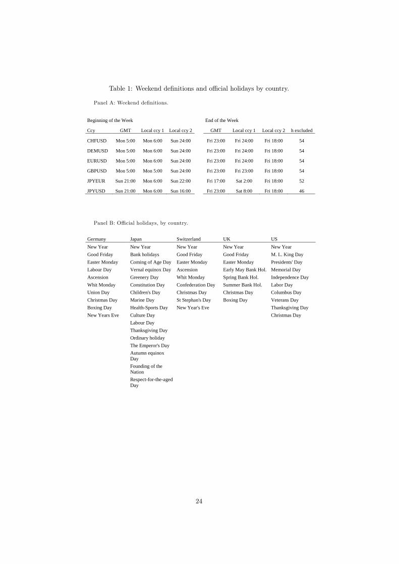
Table 1: Weekend definitions and official holidays by country.

Panel A: Weekend definitions.

Beginning of the Week End of the Week

Ccy GMT Local ccy 1 Local ccy 2 GMT Local ccy 1 Local ccy 2 h excluded

CHFUSD Mon 5:00 Mon 6:00 Sun 24:00 Fri 23:00 Fri 24:00 Fri 18:00 54

DEMUSD Mon 5:00 Mon 6:00 Sun 24:00 Fri 23:00 Fri 24:00 Fri 18:00 54

EURUSD Mon 5:00 Mon 6:00 Sun 24:00 Fri 23:00 Fri 24:00 Fri 18:00 54

GBPUSD Mon 5:00 Mon 5:00 Sun 24:00 Fri 23:00 Fri 23:00 Fri 18:00 54

JPYEUR Sun 21:00 Mon 6:00 Sun 22:00 Fri 17:00 Sat 2:00 Fri 18:00 52

JPYUSD Sun 21:00 Mon 6:00 Sun 16:00 Fri 23:00 Sat 8:00 Fri 18:00 46

Panel B: Official holidays, by country.

Germany Japan Switzerland UK US New Year New Year New Year New Year New Year Good Friday Bank holidays Good Friday Good Friday M. L. King Day Easter Monday Coming of Age Day Easter Monday Easter Monday Presidents' Day Labour Day Vernal equinox Day Ascension Early May Bank Hol. Memorial Day Ascension Greenery Day Whit Monday Spring Bank Hol. Independence Day Whit Monday Constitution Day Confederation Day Summer Bank Hol. Labor Day Union Day Children's Day Christmas Day Christmas Day Columbus Day Christmas Day Marine Day St Stephan's Day Boxing Day Veterans Day Boxing Day Health-Sports Day New Year's Eve Thanksgiving Day New Years Eve Culture Day Christmas Day Labour Day Thanksgiving Day Ordinary holiday The Emperor's Day

Autumn equinox Day

Founding of the Nation

Respect-for-the-aged Day

24

Table 2: Descriptive statistics on CHF/USD, DEM/USD and EUR/USDexchange rate returns.

This table shows the descriptive statistics for intradaily and daily returns, excluding week-ends, for CHF/USD, DEM/USD and EUR/USD currency pairs. Intraday (log) returns arecalculated over non-overlapping 4-hour periods and then annualised by multiplying by 260.The first row shows the time of the day (GMT) and the second row indicates which countryor region is working during the different hours of the day. "Freq. Up" means the proportionof positive returns (in %). The table shows the t -test and Chi-square for testing the nullhypothesis that there is equality in means and medians, and Q-statistic for testing the nullhypothesis that there is no autocorrelation at lag 1. The Sign Test assesses the null hypothesisthat positive and negative returns are proportionally equally represented. Significance at 1%,5% and 10% is denoted by ***, ** and *, respectively.

EST 19-23 23-3 3-7 7-11 11-15 15-19 Whole GMT 0-4 4-8 8-12 12-16 16-20 20-24 Daily Working time JP JP - EU EU EU - US US US CHF/USD Mean -1.00% 3.1%** 7.2%*** -6.1%*** -3.0%** -0.80% -0.10% Median -1.00% 2.8%*** 7.9%*** -3.9%*** 0.00% 0.00% 0.00% Maximum 2.709 2.811 4.319 7.108 4.368 2.048 7.96 Minimum -3.229 -3.585 -6.091 -5.405 -5.822 -3.885 -7.382 Std. Dev. 3.3% 5.1% 6.7% 5.4% 2.6% 2.9% 4.7% Skewness -0.12 -0.16 -0.25 -0.05 -0.25 -0.44 -0.21 Kurtosis 8.28 6.09 6.14 5.34 6.41 8.66 6.05 # of Obs 3274 3274 3274 3274 2620 2620 74652 Freq. Up 48.3* 52** 54.8** 48.3* 49.1 49.3 49.9 Q-Stat 1 2.89* 0.15 7.96*** 31.90*** 4.77** 2.58 - DEM/USD Mean 0.50% 1.60% 5.0%*** -5.8%*** 0.30% 0.30% 0.30% Median 0.80% 0.00% 3.8%*** -6.6%*** 0.80% 0.00% 0.00% Maximum 1.753 2.315 3.475 6.202 4.753 1.821 6.8 Minimum -2.49 -3.212 -4.447 -4.849 -4.928 -2.95 -5.763 Std. Dev. 2.7% 4.1% 5.7% 5.0% 2.5% 2.8% 4.1% Skewness -0.34 0.08 -0.03 0.22 -0.27 -0.75 -0.1 Kurtosis 6.7 6.54 7.15 6.83 8.71 10.65 7.63 # of Obs 1250 1561 1561 1561 1561 1249 35595 Freq. Up 50.1 52.1** 53.6*** 46.5*** 50.1 51.0 50.2 Q-Stat 1 1.07 0.02 27.86*** 18.86*** 6.51** 0.87 - EUR/USD Mean -1.40% -3.10% 10.3%*** -2.30% -6.4%*** 1.50% -0.30% Median 0.00% -1.4%* 10.8%*** 1.40% -5.7%*** 1.10% 0.00% Maximum 2.569 2.758 4.034 3.433 4.313 1.641 5.072 Minimum -1.751 -3.732 -4.15 -4.645 -4.828 -2.379 -8.956 Std. Dev. 3.2% 5.1% 6.2% 4.6% 2.4% 2.7% 4.4% Skewness 0.2 -0.38 -0.14 -0.21 -0.14 -0.06 -0.22 Kurtosis 6.29 6.67 5.31 4.4 6.41 6.08 5.49 # of Obs 1371 1713 1713 1713 1713 1371 39060 Freq. Up 49.6 48.3* 57.3*** 50.6 46.1*** 51.3 49.9 Q-Stat 1 0.22 3.48* 0.01 19.70*** 0.83 1.24 -

25

Table 3: Descriptive statistics on GBP/USD, JPY/EUR and JPY/USDexchange rate returns.

This table shows the descriptive statistics for intradaily and daily returns, excluding week-ends, for GBP/USD, JPY/EUR and JPY/USD currency pairs. Intraday (log) returns arecalculated over non-overlapping 4-hour periods and then annualised by multiplying by 260.The first row shows the time of the day (GMT) and the second row indicates which countryor region is working during the different hours of the day. "Freq. Up" means the proportionof positive returns (in %). The table shows the t -test and Chi-square for testing the nullhypothesis that there is equality in means and medians, and Q-statistic for testing the nullhypothesis that there is no autocorrelation at lag 1. The Sign Test assesses the null hypothesisthat positive and negative returns are proportionally equally represented. Significance at 1%,5% and 10% is denoted by ***, ** and *, respectively.

EST 19-23 23-3 3-7 7-11 11-15 15-19 Whole GMT 0-4 4-8 8-12 12-16 16-20 20-24 Daily Working time JP JP - EU EU EU - US US US GBP/USD Mean -1.0% 3.4%*** 2.4%*** -3.5%*** -5.0%*** -2.8%*** -0.3% Median -0.9% 2.4%*** 2.4%*** -2.7%*** -3.7%*** 2.6%*** 0.0% Maximum 2.450 3.017 3.935 5.135 3.865 2.807 5.135 Minimum -1.831 -3.009 -3.785 -4.319 -5.002 -1.294 -5.002 Std. Dev. 2.1% 2.9% 4.1% 5.1% 3.7% 1.9% 3.5% Skewness 0.05 0.20 0.03 -0.09 -0.11 0.27 -0.06 Kurtosis 6.77 6.12 5.76 5.59 10.22 7.65 8.67 # of Obs 2623 3281 3281 3281 3281 2621 75452 Freq. Up 47*** 51.8* 52.5*** 47.5*** 45.2*** 53.3*** 49.7 Q-Stat 1 0.06 6.07** 1.04 30.69*** 0.16 0.00 - JPY/EUR Mean 2.8%* -2.80% -8.0%*** -0.90% 6.2%*** 0.10% -0.60% Median 1.30% -1.4%* -4.2%*** 0.00% 5.7%*** 0.90% 0.00% Maximum 4.791 4.961 4.239 5.525 3.88 4.627 8.942 Minimum -7.435 -4.56 -5.09 -4.791 -6.033 -9.409 -9.409 Std. Dev. 4.2% 6.0% 6.4% 4.8% 3.5% 4.6% 4.9% Skewness -0.07 -0.01 -0.33 -0.08 -0.31 -2.68 -0.18 Kurtosis 13.16 8.23 5.96 5.51 8.26 51.72 7.3 # of Obs 1713 1713 1713 1713 1370 1712 39836 Freq. Up 51.5 48.2 47.7** 50.2 54.1*** 51.5 50.3 Q-Stat 1 2.91 0.64 0.03 7.70*** 0.95 0.55 - JPY/USD Mean 2.7%** -2.40% -0.60% -4.0%*** 2.8%** 0.30% -0.20% Median 1.3%* -1.3%* 0.00% -3.7%*** 2.5%** 1.10% 0.00% Maximum 5.521 4.587 7.894 6.045 9.862 5.384 14.365 Minimum -9.998 -6.118 -15.034 -8.348 -8.773 -4.153 -21.739 Std. Dev. 3.9% 5.4% 5.1% 5.3% 3.3% 4.8% 4.7% Skewness -0.66 -0.34 -1.89 -0.42 -0.04 -0.32 -0.75 Kurtosis 17.4 13.63 39.72 11.03 15.18 15.02 24.96 # of Obs 3274 3274 3274 3274 3274 3597 79219 Freq. Up 51.2 47.9** 50.3 47.8*** 50.2 51.2 50.3 Q-Stat 1 11.26*** 9.43*** 0.04 8.87*** 4.12** 0 -

26

Table 4: Four-hour returns patterns across working days.

For each currency pair, this table shows average daily and intradaily returns during the workingweek. The table shows the t -test for testing the null hypothesis that there is equality in meansbetween the average return over a specific 4-hour period of a given day of the week and theaverage return during the same intraday period of all the working days. Significance at 1%and 5% is denoted by ** and *, respectively.

CHF/USD Mon Tue Wed Thu Fri Intraday From 0 to 4 0.90% -1.20% -4.00% 1.20% -1.00% From 4 to 8 2.90% 1.80% 2.60% 2.60% 5.00% 2.40% From 8 to 12 10.2%* 2.4%* 3.40% 6.90% 7.00% 7.20% From 12 to 16 -4.60% -3.40% -0.80% -7.10% -7.00% -5.20% From 16 to 20 -2.20% -6.5%* -1.30% -7.9%** 1.1%** -3.20% From 20 to 24 -0.30% -0.50% -0.40% -2.30% -0.80% Day-effect 1.20% -0.80% 0.40% -1.90% 0.80% 0.00% DEM/USD Mon Tue Wed Thu Fri Intraday From 0 to 4 1.80% 0.10% -3.00% 3.20% 0.50% From 4 to 8 3.60% 1.10% -0.80% -2.20% 6.50% 1.60% From 8 to 12 7.70% -0.10% 9.7%** 6.80% 1.0%* 5.00% From 12 to 16 -11.7%** 1.7%** -4.80% -6.00% -8.30% -5.80% From 16 to 20 3.20% -1.20% 0.70% -10.8%** 9.8%** 0.30% From 20 to 24 -1.30% 1.40% 1.30% -0.30% 0.30% Day-effect 0.50% 0.40% 0.90% -2.70% 2.30% 0.00% EUR/USD Mon Tue Wed Thu Fri Intraday From 0 to 4 1.00% -2.70% -3.10% -0.60% -1.40% From 4 to 8 -5.20% -3.90% -6.10% -0.60% 0.50% -3.10% From 8 to 12 13.7%* 8.70% 14.6%** 9.30% 5.3%** 10.30% From 12 to 16 1.5%* -10.5%** 2.6%* -4.70% -0.70% -2.30% From 16 to 20 -5.80% -7.40% -3.90% -8.70% -6.20% -6.40% From 20 to 24 4.40% -0.20% 2.90% -1.00% 1.50% Day-effect 1.10% -1.60% 1.00% -1.00% -0.80% 0.00% GBP/USD Mon Tue Wed Thu Fri Intraday From 0 to 4 -0.7% -2.2% -1.6% 0.6% -1.0% From 4 to 8 1.6% 3.0% 4.3% 2.4% 5.4% 3.4% From 8 to 12 2.7% 1.1% 4.7%** 1.3% 2.4% 2.4% From 12 to 16 -2.2% -1.8% -1.7% -9.7%** -2.1% -3.5% From 16 to 20 -2.9% -5.7% -4.5% -10.5%** -1.2% -5.0% From 20 to 24 2.3% 2.5% 2.4% 3.9% 2.8% Day-effect -0.6% -0.1% 0.4% -2.4% 1.2% -0.3% JPY/EUR Mon Tue Wed Thu Fri Intraday From 0 to 4 -3.7%* 3.40% 2.50% 1.50% 10.5%** 2.90% From 4 to 8 -1.70% -0.20% -0.40% -7.1%* -4.50% -2.80% From 8 to 12 -15.7%** -7.40% -5.70% -5.10% -5.30% -7.80% From 12 to 16 2.8%** 1.60% -5.7%** 1.50% -4.6%* -0.90% From 16 to 20 6.10% -0.10% 8.00% 10.90% 6.20% From 20 to 24 0.50% 2.40% -1.90% 6.70% 0.20% Day-effect -2.60% 0.00% -0.10% 0.10% 0.50% -0.60% JPY/EUR Mon Tue Wed Thu Fri Intraday From 0 to 4 -1.5%* 2.60% 2.50% -3.5%** 13.6%** 2.70% From 4 to 8 -2.40% -3.00% -4.50% -0.10% -1.80% -2.50% From 8 to 12 0.40% 0.80% 3.4%** -3.30% -4.5%* -0.60% From 12 to 16 -5.20% -4.80% -0.70% -8.1%** -1.00% -4.00% From 16 to 20 4.70% -5.8%** 4.60% 3.90% 6.6%* 2.80% From 20 to 24 2.50% -1.90% 0.50% -0.60% -0.40% 0.30% Day-effect -0.50% -1.80% 1.10% -2.20% 2.50% 0.00%

27

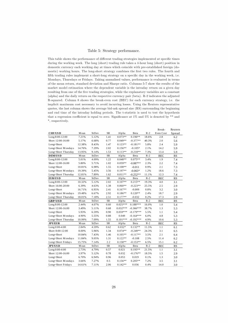
Table 5: Strategy performance.

This table shows the performance of different trading strategies implemented at specific timesduring the working week. The long (short) trading rule takes a 4-hour long (short) position indomestic currency each working day at times which coincide with pre-established foreign (do-mestic) working hours. The long-short strategy combines the first two rules. The fourth andfifth trading rules implement a short-long strategy on a specific day in the working week, i.e.Mondays, Thursdays or Fridays. Taking annualised values, performance is evaluated in termsof the mean return, standard deviation and Sharpe ratio. Columns 5-7 show the results of themarket model estimation where the dependent variable is the intraday return on a given dayresulting from one of the five trading strategies, while the explanatory variables are a constant(alpha) and the daily return on the respective currency pair (beta). R-2 indicates the adjustedR-squared. Column 8 shows the break-even cost (BEC) for each currency strategy, i.e. theimplicit maximum cost necessary to avoid incurring losses. Using the Reuters representativequotes, the last column shows the average bid-ask spread size (RS) surrounding the beginningand end time of the intraday holding periods. The t-statistic is used to test the hypothesisthat a regression coefficient is equal to zero. Significance at 1% and 5% is denoted by ** and*, respectively.

CHF/US D M ean StDev SR Alp ha Beta R-2

Break-Even Cost

Reuters Spread

Long 8:00-12:00 7.21% 5.12% 1.41 0.073** 0.196** 18.6% 2.8 6.2Short 12:00-16:00 5.17% 6.68% 0.77 0.049** -0.377** 40.3% 2.0 5.6Long+Short 12.38% 8.43% 1.47 0.123** -0.181** 5.8% 2.4 5.9Long+Short M onday s 14.76% 7.29% 2.02 0.156** -0.105* 2.1% 14.2 5.9Long+Short Thursday 13.95% 9.14% 1.53 0.113** -0.218** 7.3% 13.4 5.9DEM/US D M ean StDev SR Alp ha Beta R-2 BEC RSLong 8:00-12:00 5.01% 4.09% 1.22 0.048** 0.075** 3.4% 1.9 7.4Short 12:00-16:00 5.80% 5.71% 1.02 0.059** -0.087** 2.3% 2.2 7.4Long+Short 10.81% 6.98% 1.55 0.108** -0.011 0.9% 2.1 7.3Long+Short M onday s 19.39% 5.45% 3.56 0.197** -0.065* 1.2% 18.6 7.3Long+Short Thursday 12.81% 7.89% 1.62 0.011** -0.252** 11.1% 12.3 7.4EUR/US D M ean StDev SR Alp ha Beta R-2 BEC RSLong 8:00-12:00 10.32% 5.12% 2.02 0.107** 0.215** 19.3% 4.0 3.1Short 16:00-20:00 6.39% 4.63% 1.38 0.060** -0.223** 25.5% 2.5 2.9Long+Short 16.71% 6.95% 2.41 0.167** -0.009 0.8% 3.2 3.0Long+Short M onday s 19.48% 6.67% 2.92 0.186** 0.120** 2.4% 18.7 2.9Long+Short Thursday 18.01% 7.18% 2.51 0.177** -0.032 0.2% 17.3 2.9GBP/USD M ean StDev SR Alp ha Beta R-2 BEC RSLong 8:00-12:00 2.44% 4.07% 0.60 0.025*** 0.188*** 16.0% 1.0 5.4Short 12:00-16:00 3.49% 5.11% 0.68 0.032*** -0.366*** 38.7% 1.3 5.3Long+Short 5.93% 6.59% 0.90 0.059*** -0.179*** 5.5% 1.1 5.4Long+Short M onday s 4.90% 5.55% 0.88 0.049 -0.164*** 6.0% 4.8 5.3Long+Short Thursday 10.99% 7.09% 1.55 0.101*** -0.192*** 4.9% 10.6 5.3JPY/EUR M ean StDev SR Alp ha Beta R-2 BEC RSLong 0:00-4:00 2.84% 4.59% 0.62 0.032* 0.132** 11.5% 1.1 6.1Short 8:00-12:00 8.00% 5.96% 1.34 0.074** -0.249** 24.3% 3.1 6.5Long+Short 10.84% 7.43% 1.46 0.105** -0.117** 3.5% 2.1 6.4Long+Short M onday s 11.84% 9.05% 1.31 0.122** -0.108 2.5% 11.4 6.2Long+Short Friday s 15.75% 7.14% 2.2 0.158** -0.153** 6.5% 15.1 6.2JPY/US D M ean StDev SR Alp ha Beta R-2 BEC RSLong 0:00-4:00 2.73% 4.79% 0.57 0.021 0.195** 21.5% 1.1 3.1Short 12:00-16:00 3.97% 5.12% 0.78 0.032 -0.176** 18.5% 1.5 2.9Long+Short 6.70% 6.94% 0.96 0.053 0.019 0.1% 1.3 3.0Long+Short M onday s 3.66% 7.27% 0.5 0.156** 0.205** 7.2% 3.5 3.1Long+Short Friday s 14.61% 7.11% 2.06 0.142** 0.036 0.4% 14.0 3.0

28

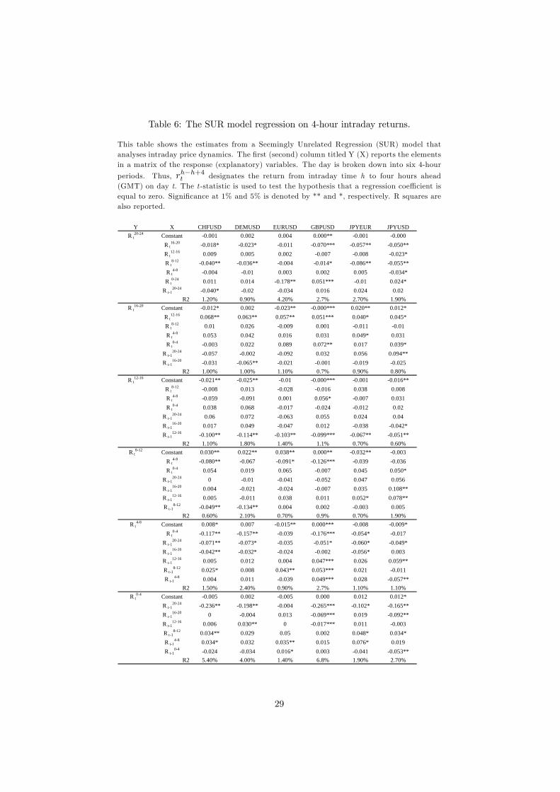
Table 6: The SUR model regression on 4-hour intraday returns.

This table shows the estimates from a Seemingly Unrelated Regression (SUR) model thatanalyses intraday price dynamics. The first (second) column titled Y (X) reports the elementsin a matrix of the response (explanatory) variables. The day is broken down into six 4-hour

periods. Thus, rh−h+4t designates the return from intraday time h to four hours ahead(GMT) on day t. The t -statistic is used to test the hypothesis that a regression coefficient isequal to zero. Significance at 1% and 5% is denoted by ** and *, respectively. R squares arealso reported.

Y X CHFUSD DEMUSD EURUSD GBPUSD JPYEUR JPYUSDR t

20-24 Constant -0.001 0.002 0.004 0.000** -0.001 -0.000R t

16-20 -0.018* -0.023* -0.011 -0.070*** -0.057** -0.050**R t

12-16 0.009 0.005 0.002 -0.007 -0.008 -0.023*R t

8-12 -0.040** -0.036** -0.004 -0.014* -0.086** -0.055**R t

4-8 -0.004 -0.01 0.003 0.002 0.005 -0.034*R t

0-24 0.011 0.014 -0.178** 0.051*** -0.01 0.024*R t-1

20-24 -0.040* -0.02 -0.034 0.016 0.024 0.02R2 1.20% 0.90% 4.20% 2.7% 2.70% 1.90%

R t16-20 Constant -0.012* 0.002 -0.023** -0.000*** 0.020** 0.012*

R t12-16 0.068** 0.063** 0.057** 0.051*** 0.040* 0.045*

R t8-12 0.01 0.026 -0.009 0.001 -0.011 -0.01

R t4-8 0.053 0.042 0.016 0.031 0.049* 0.031

R t0-4 -0.003 0.022 0.089 0.072** 0.017 0.039*

R t-120-24 -0.057 -0.002 -0.092 0.032 0.056 0.094**

R t-116-20 -0.031 -0.065** -0.021 -0.001 -0.019 -0.025

R2 1.00% 1.00% 1.10% 0.7% 0.90% 0.80%R t

12-16 Constant -0.021** -0.025** -0.01 -0.000*** -0.001 -0.016**R t

8-12 -0.008 0.013 -0.028 -0.016 0.038 0.008R t

4-8 -0.059 -0.091 0.001 0.056* -0.007 0.031R t

0-4 0.038 0.068 -0.017 -0.024 -0.012 0.02R t-1

20-24 0.06 0.072 -0.063 0.055 0.024 0.04R t-1

16-20 0.017 0.049 -0.047 0.012 -0.038 -0.042*R t-1

12-16 -0.100** -0.114** -0.103** -0.099*** -0.067** -0.051**R2 1.10% 1.80% 1.40% 1.1% 0.70% 0.60%

R t8-12 Constant 0.030** 0.022** 0.038** 0.000** -0.032** -0.003

R t4-8 -0.080** -0.067 -0.091* -0.126*** -0.039 -0.036

R t0-4 0.054 0.019 0.065 -0.007 0.045 0.050*

R t-120-24 0 -0.01 -0.041 -0.052 0.047 0.056

R t-116-20 0.004 -0.021 -0.024 -0.007 0.035 0.108**

R t-112-16 0.005 -0.011 0.038 0.011 0.052* 0.078**

R t-18-12 -0.049** -0.134** 0.004 0.002 -0.003 0.005

R2 0.60% 2.10% 0.70% 0.9% 0.70% 1.90%R t

4-8 Constant 0.008* 0.007 -0.015** 0.000*** -0.008 -0.009*R t

0-4 -0.117** -0.157** -0.039 -0.176*** -0.054* -0.017R t-1

20-24 -0.071** -0.073* -0.035 -0.051* -0.060* -0.049*R t-1

16-20 -0.042** -0.032* -0.024 -0.002 -0.056* 0.003R t-1

12-16 0.005 0.012 0.004 0.047*** 0.026 0.059**R t-1

8-12 0.025* 0.008 0.043** 0.053*** 0.021 -0.011R t-1

4-8 0.004 0.011 -0.039 0.049*** 0.028 -0.057**R2 1.50% 2.40% 0.90% 2.7% 1.10% 1.10%

R t0-4 Constant -0.005 0.002 -0.005 0.000 0.012 0.012*

R t-120-24 -0.236** -0.198** -0.004 -0.265*** -0.102* -0.165**

R t-116-20 0 -0.004 0.013 -0.069*** 0.019 -0.092**

R t-112-16 0.006 0.030** 0 -0.017*** 0.011 -0.003

R t-18-12 0.034** 0.029 0.05 0.002 0.048* 0.034*

R t-14-8 0.034* 0.032 0.035** 0.015 0.076* 0.019

R t-10-4 -0.024 -0.034 0.016* 0.003 -0.041 -0.053**

R2 5.40% 4.00% 1.40% 6.8% 1.90% 2.70%

29

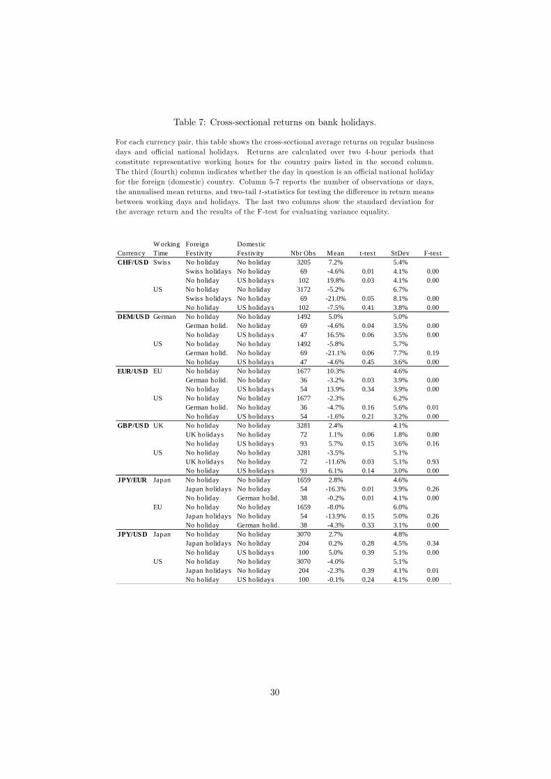
Table 7: Cross-sectional returns on bank holidays.

For each currency pair, this table shows the cross-sectional average returns on regular businessdays and official national holidays. Returns are calculated over two 4-hour periods thatconstitute representative working hours for the country pairs listed in the second column.The third (fourth) column indicates whether the day in question is an official national holidayfor the foreign (domestic) country. Column 5-7 reports the number of observations or days,the annualised mean returns, and two-tail t -statistics for testing the difference in return meansbetween working days and holidays. The last two columns show the standard deviation forthe average return and the results of the F-test for evaluating variance equality.

Currency

W orking Time

Foreign Fes tivity

Domes tic Fes tivity Nbr Obs Mean t-tes t StDev F-tes t

CHF/USD Swis s No holiday No holiday 3205 7.2% 5.4%Swiss holidays No holiday 69 -4.6% 0.01 4.1% 0.00No holiday US holidays 102 19.8% 0.03 4.1% 0.00

US No holiday No holiday 3172 -5.2% 6.7%Swiss holidays No holiday 69 -21.0% 0.05 8.1% 0.00No holiday US holidays 102 -7.5% 0.41 3.8% 0.00

DEM/USD German No holiday No holiday 1492 5.0% 5.0%German holid. No holiday 69 -4.6% 0.04 3.5% 0.00No holiday US holidays 47 16.5% 0.06 3.5% 0.00

US No holiday No holiday 1492 -5.8% 5.7%German holid. No holiday 69 -21.1% 0.06 7.7% 0.19No holiday US holidays 47 -4.6% 0.45 3.6% 0.00

EUR/USD EU No holiday No holiday 1677 10.3% 4.6%German holid. No holiday 36 -3.2% 0.03 3.9% 0.00No holiday US holidays 54 13.9% 0.34 3.9% 0.00

US No holiday No holiday 1677 -2.3% 6.2%German holid. No holiday 36 -4.7% 0.16 5.6% 0.01No holiday US holidays 54 -1.6% 0.21 3.2% 0.00

GBP/USD UK No holiday No holiday 3281 2.4% 4.1%UK holidays No holiday 72 1.1% 0.06 1.8% 0.00No holiday US holidays 93 5.7% 0.15 3.6% 0.16

US No holiday No holiday 3281 -3.5% 5.1%UK holidays No holiday 72 -11.6% 0.03 5.1% 0.93No holiday US holidays 93 6.1% 0.14 3.0% 0.00

JPY/EUR Japan No holiday No holiday 1659 2.8% 4.6%Japan holidays No holiday 54 -16.3% 0.01 3.9% 0.26No holiday German holid. 38 -0.2% 0.01 4.1% 0.00

EU No holiday No holiday 1659 -8.0% 6.0%Japan holidays No holiday 54 -13.9% 0.15 5.0% 0.26No holiday German holid. 38 -4.3% 0.33 3.1% 0.00

JPY/USD Japan No holiday No holiday 3070 2.7% 4.8%Japan holidays No holiday 204 0.2% 0.28 4.5% 0.34No holiday US holidays 100 5.0% 0.39 5.1% 0.00

US No holiday No holiday 3070 -4.0% 5.1%Japan holidays No holiday 204 -2.3% 0.39 4.1% 0.01No holiday US holidays 100 -0.1% 0.24 4.1% 0.00 .

30

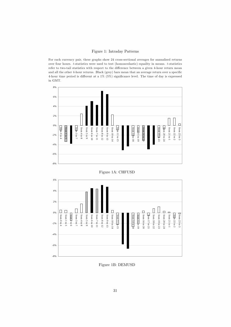
Figure 1: Intraday Patterns

For each currency pair, these graphs show 24 cross-sectional averages for annualised returnsover four hours. t -statistics were used to test (homoscedastic) equality in means. t -statisticsrefer to two-tail statistics with respect to the difference between a given 4-hour return meanand all the other 4-hour returns. Black (grey) bars mean that an average return over a specific4-hour time period is different at a 1% (5%) significance level. The time of day is expressedin GMT.

-8%

-6%

-4%

-2%

0%

2%

4%

6%

8%

from 0 to 4

from 1 to 5

from 2 to 6

from 3 to 7

from 4 to 8

from 5 to 9

from 6 to 10

from 7 to 11

from 8 to 12

from 9 to 13

from 10 to 14

from 11 to 15

from 12 to 16

from 13 to 17

from 14 to 18

from 15 to 19

from 16 to 20

from 17 to 21

from 18 to 22

from 19 to 23

from 20 to 24

from 21 to 1

from 22 to 2

from 23 to 3

Figure 1A: CHFUSD

-8%

-6%

-4%

-2%

0%

2%

4%

6%

from 0 to 4

from 1 to 5

from 2 to 6

from 3 to 7

from 4 to 8

from 5 to 9

from 6 to 10

from 7 to 11

from 8 to 12

from 9 to 13

from 10 to 14

from 11 to 15

from 12 to 16

from 13 to 17

from 14 to 18

from 15 to 19

from 16 to 20

from 17 to 21

from 18 to 22

from 19 to 23

from 20 to 24

from 21 to 1

from 22 to 2

from 23 to 3

Figure 1B: DEMUSD

31

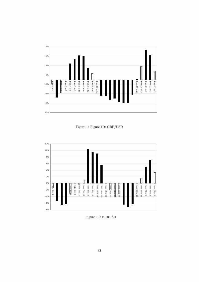
-7%

-5%

-3%

-1%

1%

3%

5%

7%

from 0 to 4

from 1 to 5

from 2 to 6

from 3 to 7

from 4 to 8

from 5 to 9

from 6 to 10

from 7 to 11

from 8 to 12

from 9 to 13

from 10 to 14

from 11 to 15

from 12 to 16

from 13 to 17

from 14 to 18

from 15 to 19

from 16 to 20

from 17 to 21

from 18 to 22

from 19 to 23

from 20 to 24

from 21 to 1

from 22 to 2

from 23 to 3

Figure 1: Figure 1D: GBP/USD

-8%

-6%

-4%

-2%

0%

2%

4%

6%

8%

10%

12%from

0 to 4

from 1 to 5

from 2 to 6

from 3 to 7

from 4 to 8

from 5 to 9

from 6 to 10

from 7 to 11

from 8 to 12

from 9 to 13

from 10 to 14

from 11 to 15

from 12 to 16

from 13 to 17

from 14 to 18

from 15 to 19

from 16 to 20

from 17 to 21

from 18 to 22

from 19 to 23

from 20 to 24

from 21 to 1

from 22 to 2

from 23 to 3

Figure 1C: EURUSD

32

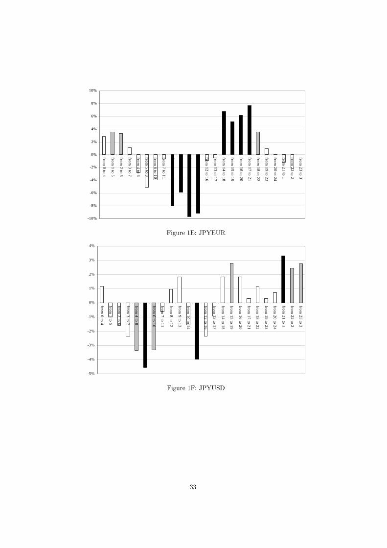
-10%

-8%

-6%

-4%

-2%

0%

2%

4%

6%

8%

10%

from 0 to 4

from 1 to 5

from 2 to 6

from 3 to 7

from 4 to 8

from 5 to 9

from 6 to 10

from 7 to 11

from 8 to 12

from 9 to 13

from 10 to 14

from 11 to 15

from 12 to 16

from 13 to 17

from 14 to 18

from 15 to 19

from 16 to 20

from 17 to 21

from 18 to 22

from 19 to 23

from 20 to 24

from 21 to 1

from 22 to 2

from 23 to 3

Figure 1E: JPYEUR

-5%

-4%

-3%

-2%

-1%

0%

1%

2%

3%

4%

from 0 to 4

from 1 to 5

from 2 to 6

from 3 to 7

from 4 to 8

from 5 to 9

from 6 to 10

from 7 to 11

from 8 to 12

from 9 to 13

from 10 to 14

from 11 to 15

from 12 to 16

from 13 to 17

from 14 to 18

from 15 to 19

from 16 to 20

from 17 to 21

from 18 to 22

from 19 to 23

from 20 to 24

from 21 to 1

from 22 to 2

from 23 to 3

Figure 1F: JPYUSD

33

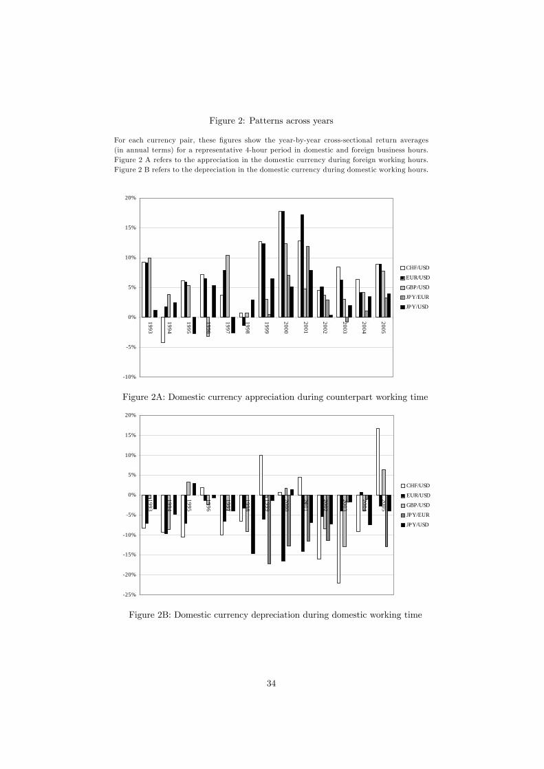
Figure 2: Patterns across years

For each currency pair, these figures show the year-by-year cross-sectional return averages(in annual terms) for a representative 4-hour period in domestic and foreign business hours.Figure 2 A refers to the appreciation in the domestic currency during foreign working hours.Figure 2 B refers to the depreciation in the domestic currency during domestic working hours.

-10%

-5%

0%

5%

10%

15%

20%

1993

1994

1995

1996

1997

1998

1999

2000

2001

2002

2003

2004

2005

CHF/USD

EUR/USD

GBP/USD

JPY/EUR

JPY/USD

Figure 2A: Domestic currency appreciation during counterpart working time

-25%

-20%

-15%

-10%

-5%

0%

5%

10%

15%

20%

1993

1994

1995

1996

1997

1998

1999

2000

2001

2002

2003

2004

2005

CHF/USD

EUR/USD

GBP/USD

JPY/EUR

JPY/USD

Figure 2B: Domestic currency depreciation during domestic working time

34