Segment 4Sampling Distributions

- or -Statistics is really just a guessing game

George Howard

Statistics as organized guessing• One of the two major tasks in statistics is

“estimation” (the technical term for guessing)• Suppose that there is some huge group of people

(or whatever we are studying)• The huge group is called the universe• This population arises from some distribution

– We have talked about arising from either binomial or normal

– Then this large population can be described by parameters

• p for the binomial• μ and σ for the normal

– Our task is to estimate (guess) the parameters

How do we estimate the parameters?

• Approach 1: measure everyone– Advantages

• You will get the correct answer– Disadvantages

• Expensive• Impractical

• Approach 2: estimation– Take a sample of the big group and try to guess– That is: we guess at the parameters in the universe

by using estimates from a sample

Characteristics of Estimates• Expectation

– We take an sample and produce estimates– We take another sample and produce

estimates again– We will get different answers

• Consider the most simple example, estimating the mean of a normal distribution (μ)

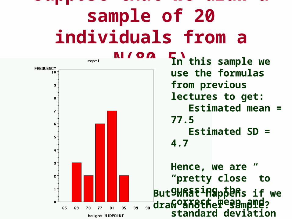
Suppose that we draw a sample of 20 individuals from a N(80,5)

In this sample we use the formulas from previous lectures to get: Estimated mean = 77.5 Estimated SD = 4.7

Hence, we are “pretty close” to guessing the correct mean and standard deviation

But what happens if we draw another sample?

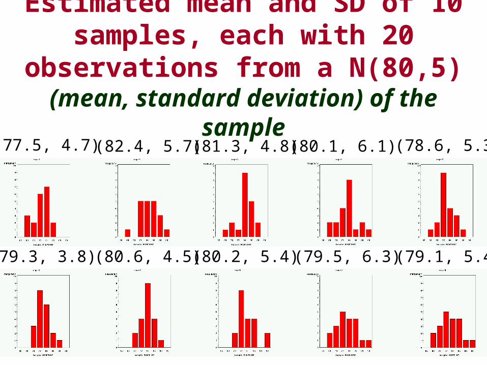
Estimated mean and SD of 10 samples, each with 20 observations from a N(80,5)

(mean, standard deviation) of the sample

(77.5, 4.7) (82.4, 5.7) (81.3, 4.8) (80.1, 6.1) (78.6, 5.3)

(79.3, 3.8) (80.6, 4.5) (80.2, 5.4) (79.5, 6.3) (79.1, 5.4)

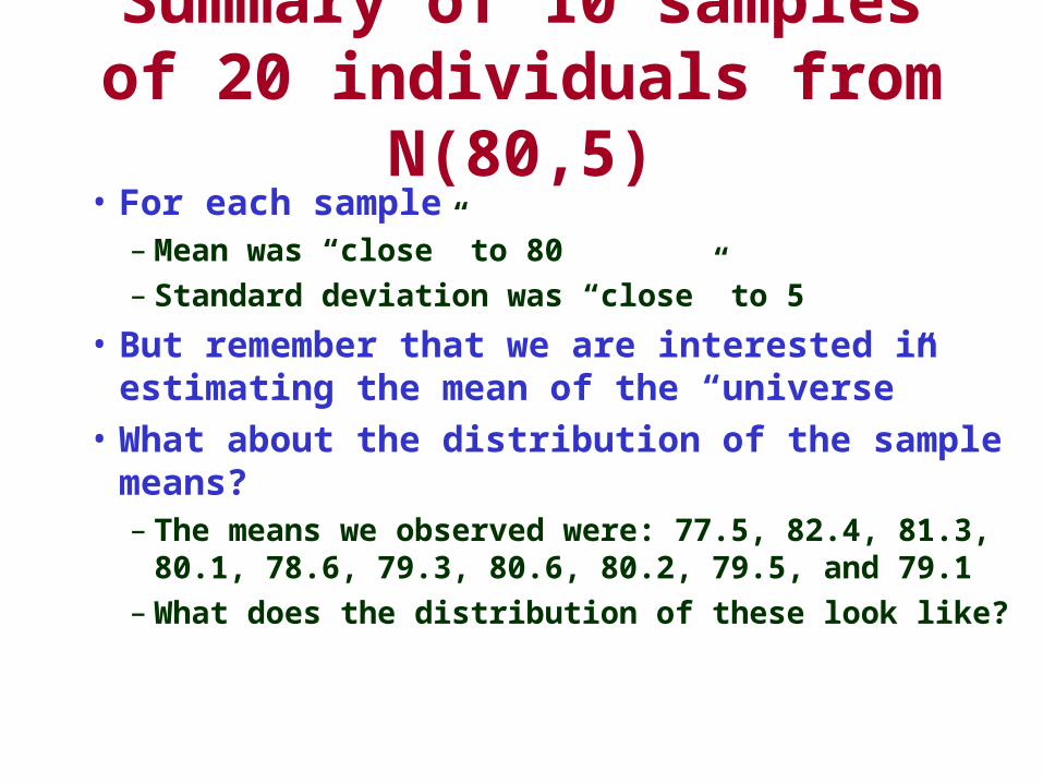
Summary of 10 samples of 20 individuals from N(80,5)

• For each sample– Mean was “close” to 80– Standard deviation was “close” to 5

• But remember that we are interested in estimating the mean of the “universe”

• What about the distribution of the sample means?– The means we observed were: 77.5, 82.4, 81.3, 80.1,

78.6, 79.3, 80.6, 80.2, 79.5, and 79.1 – What does the distribution of these look like?

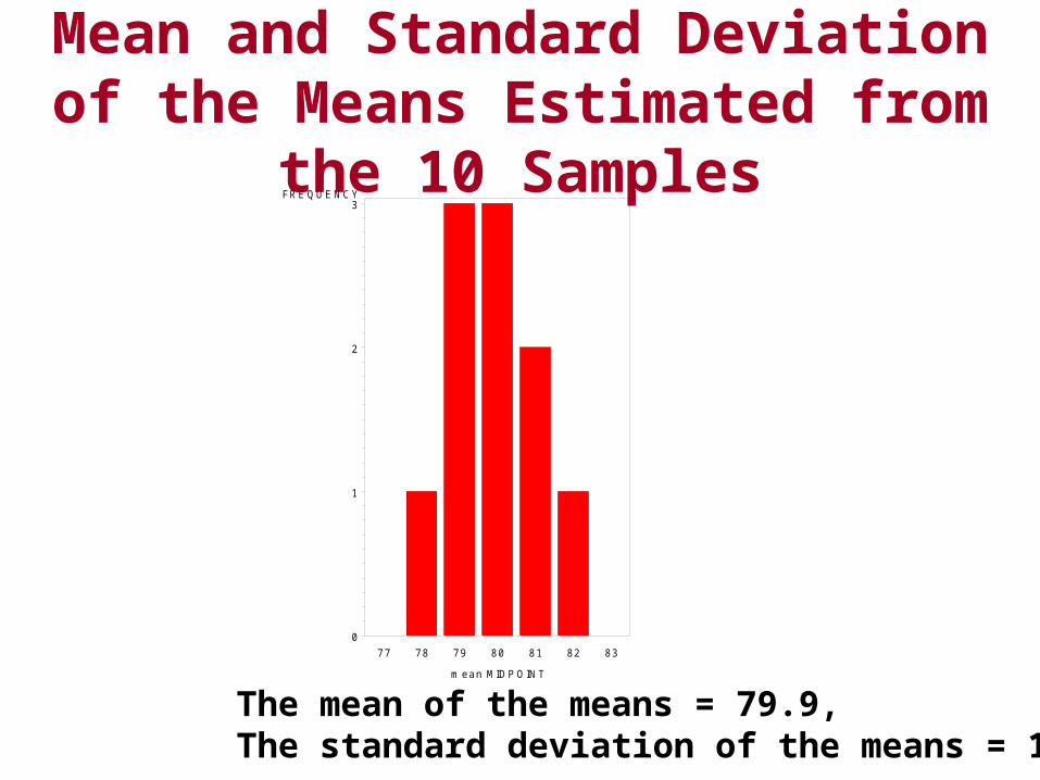
Mean and Standard Deviation of the Means Estimated from the 10 Samples

The mean of the means = 79.9, The standard deviation of the means = 1.4

FRE QUE NCY

0

1

2

3

m ean MIDP OINT

77 78 79 80 81 82 83

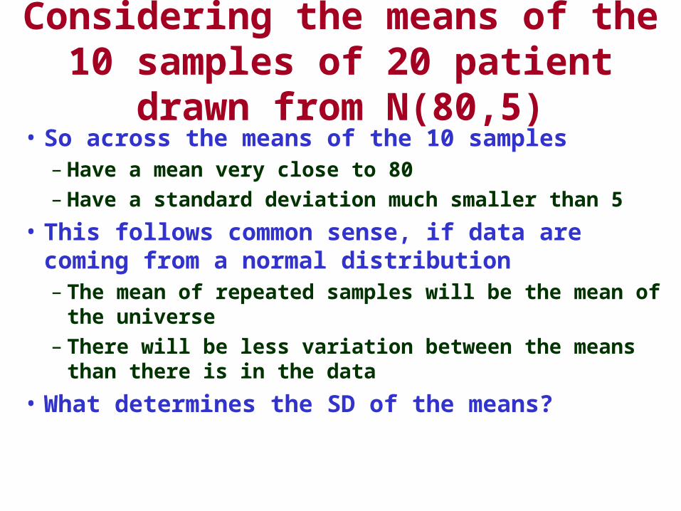
Considering the means of the 10 samples of 20 patient drawn from N(80,5)

• So across the means of the 10 samples– Have a mean very close to 80– Have a standard deviation much smaller than 5

• This follows common sense, if data are coming from a normal distribution– The mean of repeated samples will be the mean of the universe– There will be less variation between the means than there is in

the data• What determines the SD of the means?

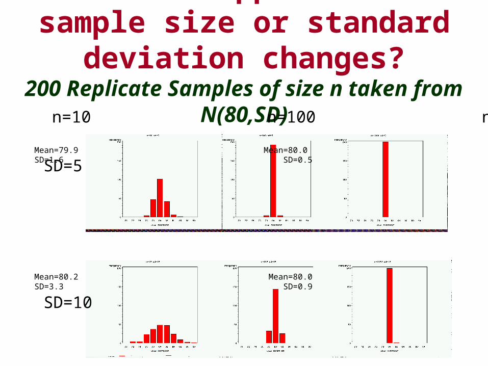
But what happens if the sample size or standard deviation changes?

200 Replicate Samples of size n taken from N(80,SD) n=10 n=100 n=1000

SD=5

SD=10

Mean=79.9 Mean=80.0 Mean=80.0SD=1.6 SD=0.5 SD=0.1

Mean=80.2 Mean=80.0 Mean=80.0SD=3.3 SD=0.9 SD=0.3

The Estimation of Parameters from a N(80,5)

• The mean of the estimated means across samples will be the same as the mean of the universe– If a estimate of a parameter is correct on average,

then we call it an unbiased estimator• The standard deviation of the estimated means

is smaller than the standard deviation of the population– But increases with the standard deviation of the

universe– Decreases with the sample size

The Standard Deviation of the Estimated Mean

• A “good” estimate of the mean should be unbiased and stable (that is, correct on average and would not change much if the experiment is repeated)

• ANY estimate has variation between repeated experiments, and “good” estimates will have small standard deviations across repeated experiments

• Estimates with low variability are called reliable (and the estimates with the smallest variation are sometimes called minimum variance estimators)

• In general we do not repeat experiments, so how can I know what the standard deviation of the estimate would be if I did repeat the experiment?

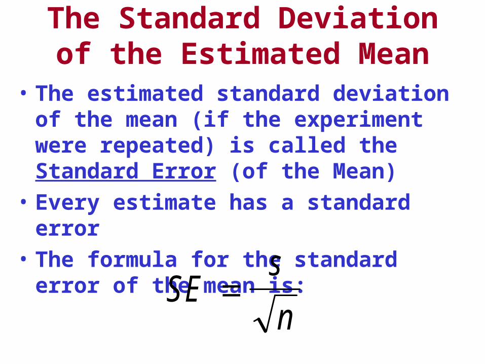
The Standard Deviation of the Estimated Mean

• The estimated standard deviation of the mean (if the experiment were repeated) is called the Standard Error (of the Mean)

• Every estimate has a standard error• The formula for the standard error of the mean

is:

SEs

n

The Standard Error

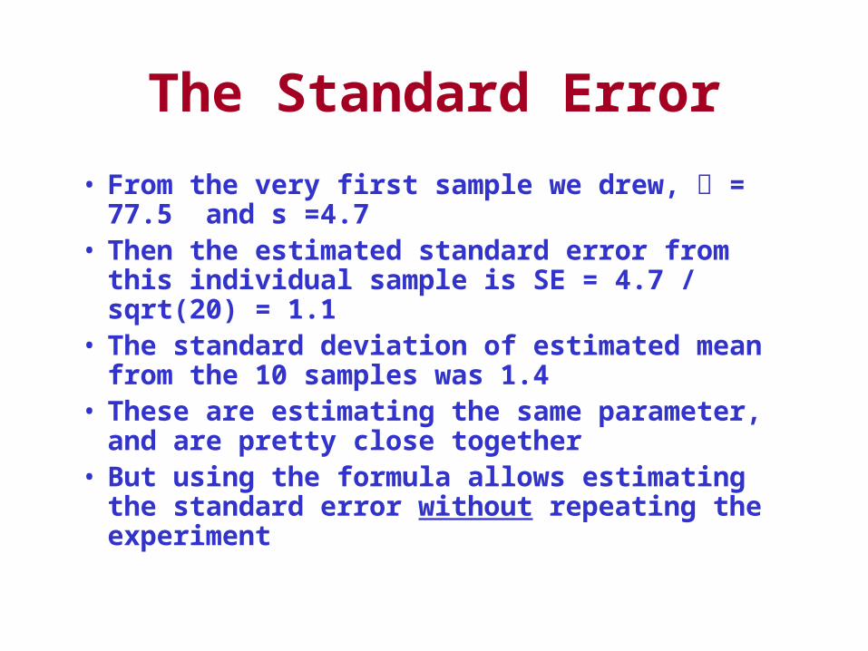
• From the very first sample we drew, = 77.5 and s =4.7

• Then the estimated standard error from this individual sample is SE = 4.7 / sqrt(20) = 1.1

• The standard deviation of estimated mean from the 10 samples was 1.4

• These are estimating the same parameter, and are pretty close together

• But using the formula allows estimating the standard error without repeating the experiment

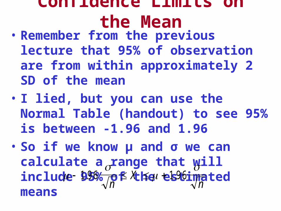
Confidence Limits on the Mean• Remember from the previous lecture that 95%

of observation are from within approximately 2 SD of the mean

• I lied, but you can use the Normal Table (handout) to see 95% is between -1.96 and 1.96

• So if we know μ and σ we can calculate a range that will include 95% of the estimated means

1 9 6 1 9 6. .n

Xn

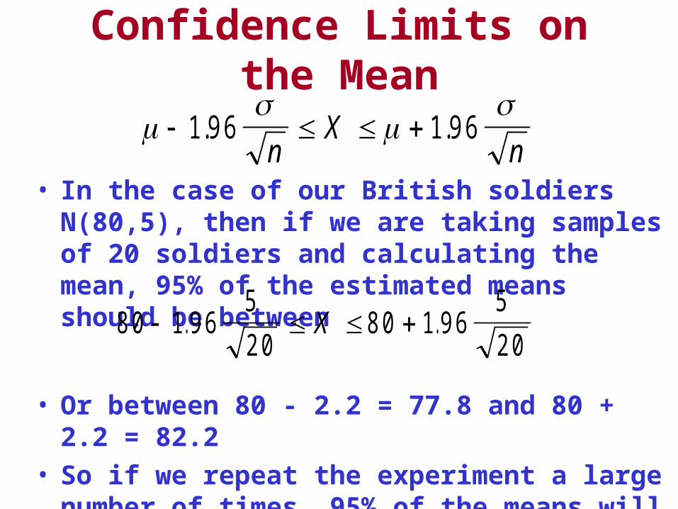
Confidence Limits on the Mean

• In the case of our British soldiers N(80,5), then if we are taking samples of 20 soldiers and calculating the mean, 95% of the estimated means should be between

1 9 6 1 9 6. .n

Xn

8 0 1 9 65

2 08 0 1 9 6

5

2 0 . .X

• Or between 80 - 2.2 = 77.8 and 80 + 2.2 = 82.2• So if we repeat the experiment a large number of

times, 95% of the means will be between 77.8 and 82.2

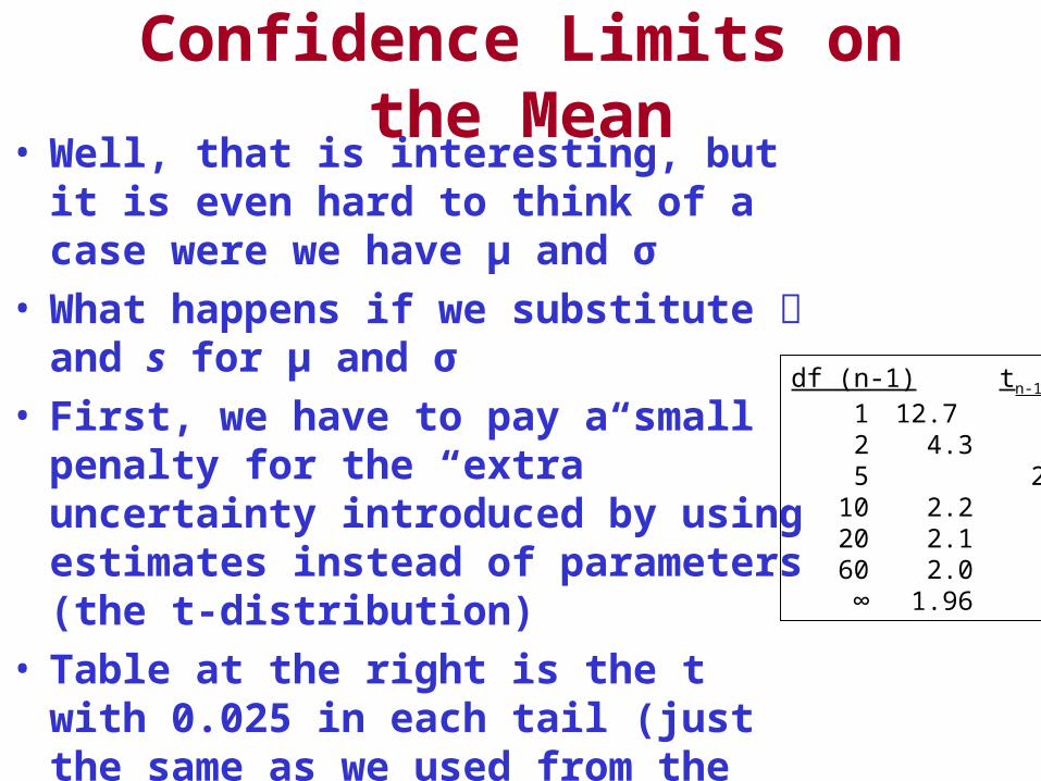
• Well, that is interesting, but it is even hard to think of a case were we have μ and σ

• What happens if we substitute and s for μ and σ

• First, we have to pay a small penalty for the “extra” uncertainty introduced by using estimates instead of parameters (the t-distribution)

• Table at the right is the t with 0.025 in each tail (just the same as we used from the normal table) and is a Table in the book

• We need to think about the interpretation

Confidence Limits on the Mean

df (n-1) tn-1

1 12.7 2 4.3 5 2.6 10 2.2 20 2.1 60 2.0 ∞ 1.96

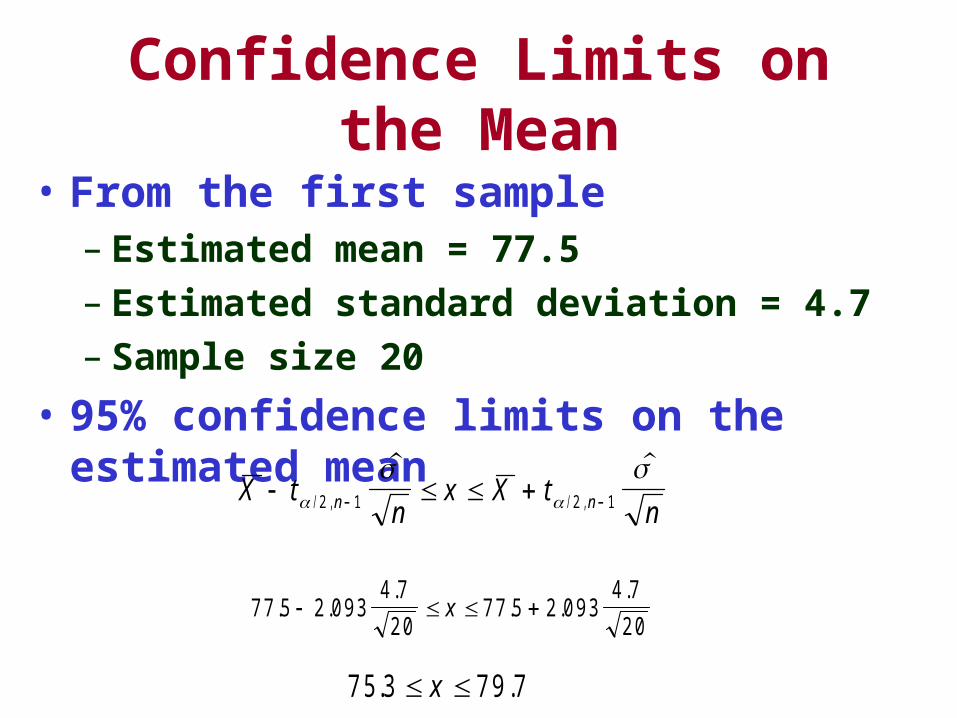
Confidence Limits on the Mean• From the first sample

– Estimated mean = 77.5– Estimated standard deviation = 4.7– Sample size 20

• 95% confidence limits on the estimated mean

X tn

x X tnn n

/ , / ,

2 1 2 1

7 7 5 2 0 9 34 7

2 07 7 5 2 0 9 3

4 7

2 0. .

.. .

. x

7 5 3 7 9 7. . x

Interpretation of the Confidence Limits on the Estimated Mean

• The 95% confidence limits are now no longer centered on the mean from the universe, but the estimated mean from the sample– We should not expect 95% of the means to fall in this

range (but rather the range centered on the true mean)– Common (and slightly incorrect) interpretation: “I am 95%

sure that the true mean is in this range”– The technically correct interpretation of 95% confidence

limits is “If I were to repeat the experiment a large number of times, and calculate confidence limits like this from each sample, 95% of the time they would include the true mean”

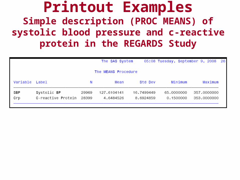
Printout ExamplesSimple description (PROC MEANS) of systolic blood

pressure and c-reactive protein in the REGARDS Study

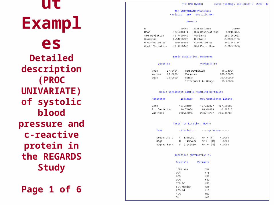
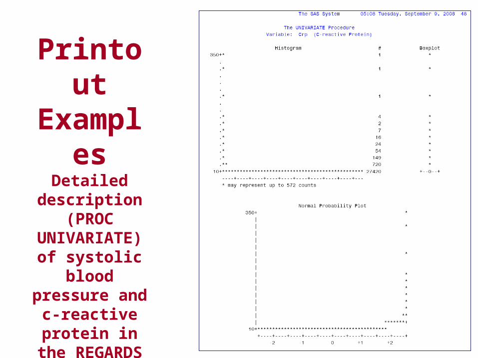
Printout Examples

Detailed description (PROC

UNIVARIATE) of systolic blood

pressure and c-reactive protein in

the REGARDS Study

Page 1 of 6

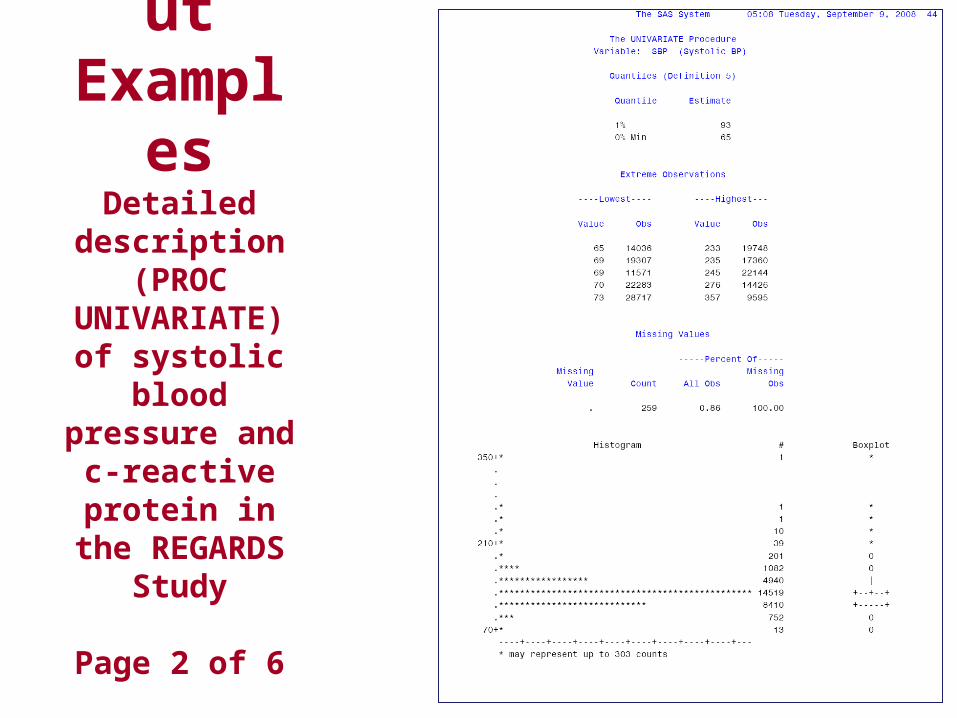
Printout Examples

Detailed description (PROC

UNIVARIATE) of systolic blood

pressure and c-reactive protein in

the REGARDS Study

Page 2 of 6

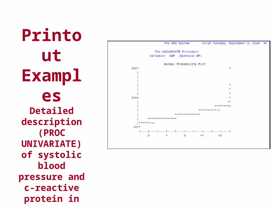
Printout Examples

Detailed description (PROC

UNIVARIATE) of systolic blood

pressure and c-reactive protein in

the REGARDS Study

Page 3 of 6

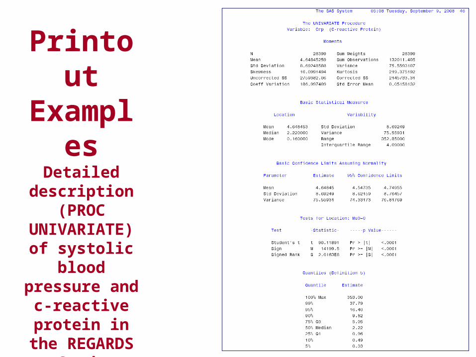
Printout Examples

Detailed description (PROC

UNIVARIATE) of systolic blood

pressure and c-reactive protein in

the REGARDS Study

Page 4 of 6

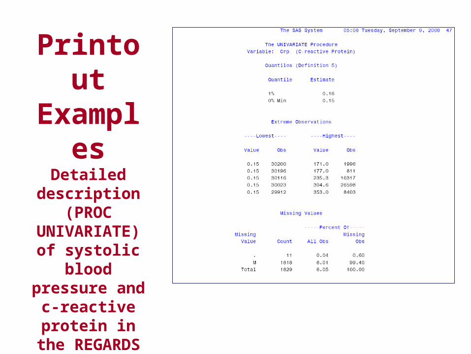
Printout Examples

Detailed description (PROC

UNIVARIATE) of systolic blood

pressure and c-reactive protein in

the REGARDS Study

Page 5 of 6

Printout Examples

Detailed description (PROC

UNIVARIATE) of systolic blood

pressure and c-reactive protein in

the REGARDS Study

Page 6 of 6

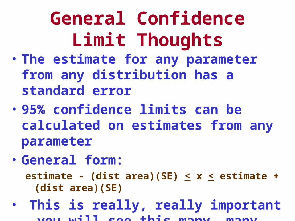
General Confidence Limit Thoughts

• The estimate for any parameter from any distribution has a standard error

• 95% confidence limits can be calculated on estimates from any parameter

• General form:estimate - (dist area)(SE) < x < estimate + (dist area)(SE)

• This is really, really important … you will see this many, many times in this course

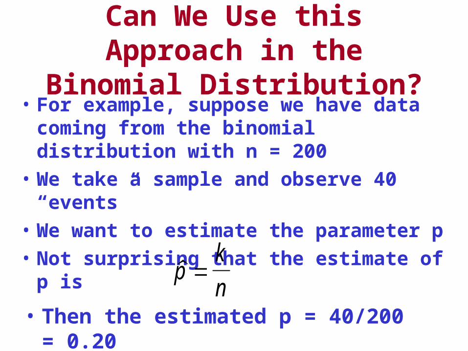
Can We Use this Approach in the Binomial Distribution?

• For example, suppose we have data coming from the binomial distribution with n = 200

• We take a sample and observe 40 “events”• We want to estimate the parameter p• Not surprising that the estimate of p is

pk

n

• Then the estimated p = 40/200 = 0.20

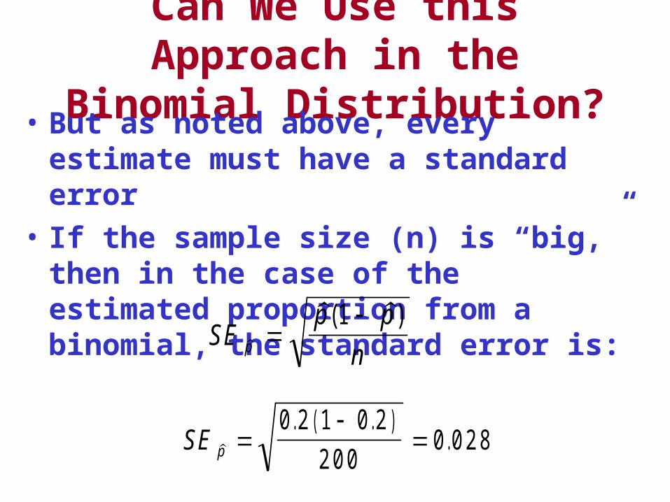
Can We Use this Approach in the Binomial Distribution?

• But as noted above, every estimate must have a standard error

• If the sample size (n) is “big,” then in the case of the estimated proportion from a binomial, the standard error is:

SEp p

np

( )

1

SE p

. ( . ).

0 2 1 0 2

2 0 00 0 2 8

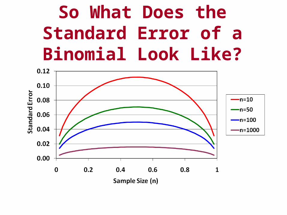
So What Does the Standard Error of a Binomial Look Like?

Can we calculate 95% confidence limits on the estimated proportion?

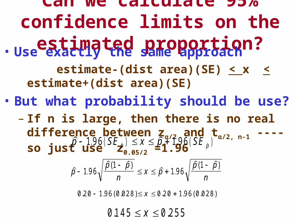
• Use exactly the same approach estimate-(dist area)(SE) < x < estimate+(dist

area)(SE)• But what probability should be use?

– If n is large, then there is no real difference between zα/2 and tα/2, n-1 ---- so just use z0.05/2 =1.96

. ( ) . ( ) p SE x p SEp p 1 9 6 1 9 6

.( )

.( )

pp p

nx p

p p

n

1 9 6

11 9 6

1

0 2 0 1 9 6 0 0 2 8 0 2 0 1 9 6 0 0 2 8. . ( . ) . . ( . ) x

0 1 4 5 0 2 5 5. . x

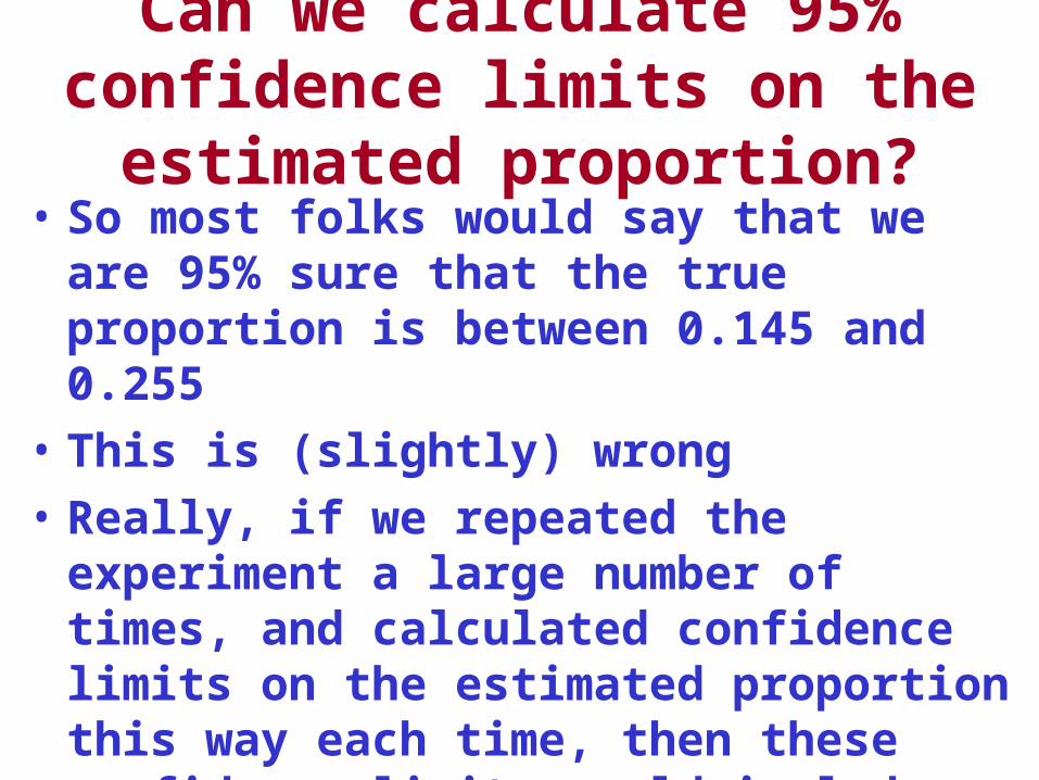
Can we calculate 95% confidence limits on the estimated proportion?

• So most folks would say that we are 95% sure that the true proportion is between 0.145 and 0.255

• This is (slightly) wrong• Really, if we repeated the experiment a large

number of times, and calculated confidence limits on the estimated proportion this way each time, then these confidence limits would include the true proportion 95% of the time

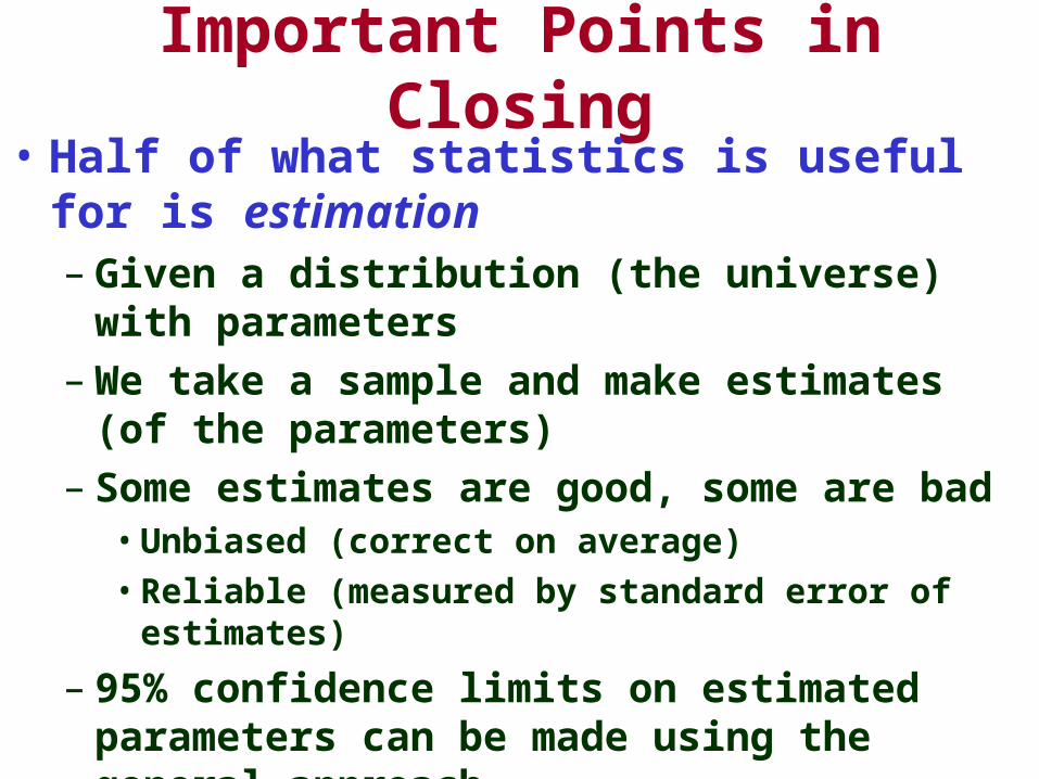
Important Points in Closing• Half of what statistics is useful for is estimation

– Given a distribution (the universe) with parameters– We take a sample and make estimates (of the

parameters)– Some estimates are good, some are bad

• Unbiased (correct on average)• Reliable (measured by standard error of estimates)

– 95% confidence limits on estimated parameters can be made using the general approach

• estimate - (dist area)(SE) < x < estimate + (dist area)(SE)– We did this for the estimated mean from a normal and

the estimated proportion from a binomial

Type of Independent Data

Categorical Continuous

Two Samples Multiple Samples

Type of Dependent Data

One Sample (focus usually on estimation) Independent Matched Independent

Repeated Measures Single Multiple

Categorical (dichotomous) 1 Estimate proportion (and confidence limits)

2 Chi-Square Test

3 McNemar Test

4 Chi Square Test

5 Generalized Estimating Equations (GEE)

6 Logistic Regression

7 Logistic Regression

Continuous 8 Estimate mean (and confidence limit)

9 Independent t-test

10 Paired t-test

11 Analysis of Variance

12 Multivariate Analysis of Variance

13 Simple linear regression & correlation coefficient

14 Multiple Regression

Right Censored (survival) 15 Kaplan Meier Survival

16 Kaplan Meier Survival for both curves, with tests of difference by Wilcoxon or log-rank test

17 Very unusual

18 Kaplan-Meier Survival for each group, with tests by generalized Wilcoxon or Generalized Log Rank

19 Very unusual

20 Proportional Hazards analysis

21 Proportional Hazards analysis

Where Have we Been Working in the “Big Picture”

1Estimate proportion (and confidence limits)

8Estimate mean (and confidence limits)