sediment metal concentrations as a function of land use in

University of Massachusetts BostonScholarWorks at UMass Boston

Graduate Doctoral Dissertations Doctoral Dissertations and Masters Theses

12-1-2012

Sediment Metal Concentrations as a Function ofLand Use in the Charles River, EasternMassachusettsDarryl L. LuceUniversity of Massachusetts Boston

Follow this and additional works at: http://scholarworks.umb.edu/doctoral_dissertations

Part of the Environmental Sciences Commons

This Open Access Dissertation is brought to you for free and open access by the Doctoral Dissertations and Masters Theses at ScholarWorks at UMassBoston. It has been accepted for inclusion in Graduate Doctoral Dissertations by an authorized administrator of ScholarWorks at UMass Boston. Formore information, please contact [email protected].

Recommended CitationLuce, Darryl L., "Sediment Metal Concentrations as a Function of Land Use in the Charles River, Eastern Massachusetts" (2012).Graduate Doctoral Dissertations. Paper 91.

http://scholarworks.umb.edu?utm_source=scholarworks.umb.edu%2Fdoctoral_dissertations%2F91&utm_medium=PDF&utm_campaign=PDFCoverPages

http://scholarworks.umb.edu/doctoral_dissertations?utm_source=scholarworks.umb.edu%2Fdoctoral_dissertations%2F91&utm_medium=PDF&utm_campaign=PDFCoverPages

http://scholarworks.umb.edu/diss_theses?utm_source=scholarworks.umb.edu%2Fdoctoral_dissertations%2F91&utm_medium=PDF&utm_campaign=PDFCoverPages

http://scholarworks.umb.edu/doctoral_dissertations?utm_source=scholarworks.umb.edu%2Fdoctoral_dissertations%2F91&utm_medium=PDF&utm_campaign=PDFCoverPages

http://network.bepress.com/hgg/discipline/167?utm_source=scholarworks.umb.edu%2Fdoctoral_dissertations%2F91&utm_medium=PDF&utm_campaign=PDFCoverPages

http://scholarworks.umb.edu/doctoral_dissertations/91?utm_source=scholarworks.umb.edu%2Fdoctoral_dissertations%2F91&utm_medium=PDF&utm_campaign=PDFCoverPages

mailto:[email protected]

SEDIMENT METAL CONCENTRATIONS AS A FUNCTION OF LAND USE IN

THE CHARLES RIVER, EASTERN MASSACHUSETTS

A Dissertation Presented

by

DARRYL L. LUCE

Submitted to the Office of Graduate Studies,

University of Massachusetts Boston,

in partial fulfillment of the requirements for the degree of

DOCTOR OF PHILOSOPHY

December 2012

Environmental, Earth and Ocean Sciences Program



A Dissertation Presented

by

DARRYL L. LUCE

Approved as to style and content by:

___________________________________________________________

Robert F. Chen, Professor

Chairperson of the Committee

___________________________________________________________

Curtis R. Olsen, Professor

Member

___________________________________________________________

William E. Robinson, Professor

Member

___________________________________________________________

Daniel Brabander, Associate Professor

Wellesley College

Member

_________________________________________

Ellen Douglas, Graduate Program Director

Department of Environmental, Earth and Ocean Sciences

_________________________________________

Robyn Hannigan, Chairperson

Department of Environmental, Earth and Ocean Sciences

v

ABSTRACT



December 2012

Darryl L. Luce, B.S., University of Missouri Kansas City

M.S., Boston College

Ph.D., University of Massachusetts Boston

Directed by Professors Gordon T. Wallace and Robert F. Chen

Two sediment cores and eleven grab samples collected from the Charles River were

analyzed to determine changes to the concentration of metals in sediments due to

anthropogenic changes in the watershed. The unique aspect of this research was that

sediment cores from the same geologic setting, yet having widely different sources, were

compared. The findings from that comparison were used to focus the investigation

through the remainder of the Charles River. The radionuclides 210

Pb, 214

Pb, and 137

Cs

established the year of deposition in the sediment cores. The concentrations of aluminum

(Al), iron (Fe), manganese (Mn), copper (Cu), zinc (Zn), chromium (Cr), cobalt (Co),

lead (Pb), arsenic (As), cadmium (Cd), tin (Sn), scandium (Sc), strontium (Sr), silver

(Ag), mercury (Hg) and total organic carbon (TOC) were determined in the sediment

cores and surface samples.

The primary findings were that several metals in Charles River sediments exceeded

regulatory standards for aquatic organisms and that storm water affected the

concentrations of metals such as Cu, Hg, and Pb throughout much of the river. What

vi

appeared critical was the retention of metals within the upland areas of a watershed which

was controlled by the amount of impervious surface. Storm water runoff from areas with

greater amounts of impervious materials, coupled with the retention of sediments behind

dams in the Charles River, increased the long-term availability of metals that may affect

aquatic organisms. A simple model is presented that determines the concentration of Cu

and Hg in sediments based on the percentage of impervious area and the concentration of

TOC in the sediment. This model indicates that a potential key to reducing the

concentrations of metals in sediments is to either reduce the amount of impervious

surfaces in a watershed or decrease the supply of metals and TOC to sediments.

vii

ACKNOWLEDGEMENTS

Work on this dissertation began in 1999 and would not have been possible without

the patience and help of my family: Catherine, my wife, and our daughters Anastacia and

Aurora. Catherine spent many hours reading and re-reading the text. My daughters can

scarcely remember any part of their lives when I was not working on this dissertation.

My advisors: Robert Chen, Curtis Olsen, Bill Robinson, and Daniel Brabander, were

invaluable to finishing this work. Their patience and guidance are appreciated. Several

students and University employees aided in the collection, processing and analysis of

samples including Elva Wohlers who assisted in sample collection and helped process

sediment cores, David Shull and Peter Edwards who collected a sediment core through

diving, Tom Goodkind who fashioned a remote sampling device, and Melissa Ferraro,

Franco Pala, Katrina Sukola, Li Li, Joe Smith and Greg Banks who were vital in assisting

me in the analytical work. None of this would have been possible without the

cooperation of the Environmental Protection Agency which supported portions of this

effort. My constant companions in writing: first George, and then Lizzy, provided

company and a friendly ear during the many long hours of writing. Lastly, I relied

heavily on the advice and guidance of Professor Gordon Wallace. I regret not being able

to consult him in the final labors of this work – he suggested this line of research and

eagerly awaited our discussions of the data. I miss the challenge and guidance he

provided.

viii

TABLE OF CONTENTS

ACKNOWLEDGEMENTS .............................................................................................. vii

LIST OF TABLES ............................................................................................................. xi

LIST OF FIGURES ......................................................................................................... xiv

LIST OF ABBREVIATIONS ......................................................................................... xvii

CHAPTER Page

1. INTRODUCTION ......................................................................................................... 1 1.1. Review of Sediment and Metal Behavior ............................................................ 5

1.1.1. Metal Sources................................................................................................ 6 1.1.1.1. Atmospheric Deposition ........................................................................ 6

1.1.1.2. Historic Anthropogenic Direct Discharges ............................................ 8 1.1.1.3. Modern Anthropogenic Sources ............................................................ 9

1.1.2. Processes that Affect Sediment Metal Concentrations ............................... 11

1.1.2.1. Dams and Waterway Management ...................................................... 11 1.1.2.2. Storm Water Management ................................................................... 15

1.1.2.3. Changes in Surface Water Metal Chemistry ....................................... 18 1.1.2.4. Changes in Sediment Metal Chemistry ............................................... 22 1.1.2.5. Biota..................................................................................................... 26

1.2. The Effect of Metals on Aquatic Life ................................................................ 27

1.3. Charles River Investigations .............................................................................. 33 1.4. Environmental Regulation.................................................................................. 34 1.5 Conclusion .......................................................................................................... 36

2. SAMPLING AND ANALYTICAL METHODS ........................................................ 39

2.1 Introduction ........................................................................................................ 39 2.2 Sampling Equipment and Collection of Samples ............................................... 39

2.3 Sediment Processing and Preparation for Analysis............................................ 44 2.3.1 Preparation for Total Organic Carbon Analysis ......................................... 45 2.3.2 Preparation for Metals Analysis.................................................................. 46 2.3.3 Preparation of Samples for Geochronology ................................................ 47

2.4 Total Organic Carbon Analysis .......................................................................... 48

2.5 Metal Analysis with Inductively Coupled Plasma – Mass Spectrometer .......... 48 2.6 Mercury Analysis via Cold Vapor Atomic Adsorption ..................................... 53

2.7 Geochronology ................................................................................................... 54

ix

CHAPTER Page

3. ECHO LAKE WATERSHED ..................................................................................... 57 Abstract ......................................................................................................................... 57

3.1 Introduction ....................................................................................................... 58 3.2 Echo Lake Study Area........................................................................................ 59

3.2.1 Echo Lake Watershed Characteristics ........................................................ 59 3.2.2 History of Land Use in Echo Lake Watershed ........................................... 61

3.3 Sediment Core Collection and Description ........................................................ 62

3.4 Results ................................................................................................................ 65 3.5 Discussion .......................................................................................................... 72

3.5.1 The Background Contribution of Metals to Sediment in Echo Lake .......... 74 3.5.2 Mercury and Lead Concentrations in Sediment before 1970 ..................... 82

3.5.3 The Supply of Metals to Echo Lake Sediment after 1970 .......................... 84 3.5.3.1. Changes in Physical Sedimentation in Echo Lake .............................. 88

3.5.3.2. Changes in Echo Lake Sediment Chemistry ....................................... 92 3.5.4 The Potential Effect of Metals in Echo Lake Sediment on Biota ............. 103

3.6 Conclusions ...................................................................................................... 105

4. BOX POND WATERSHED...................................................................................... 107

Abstract ....................................................................................................................... 107 4.1. Introduction ...................................................................................................... 108

4.2. The Box Pond Study Area ................................................................................ 110 4.3. Sediment Core Collection and Description ...................................................... 113 4.4. Results .............................................................................................................. 115

4.5 Discussion ........................................................................................................ 121

4.5.1 Anthropogenic Addition of Metals to Sediments ..................................... 122 4.5.1.1. Sources of Cr, Hg, Pb, Cd, Sn and Zn ............................................... 123 4.5.1.2. Sources of As, Cu and Ag ................................................................. 127

4.5.1.3. Sources of sediment metal trends and peaks ..................................... 130 4.5.2 The Effect of Environmental Regulation .................................................. 138

4.5.3 The Potential Effect of Box Pond Metals on Aquatic Life ....................... 139 4.6 Conclusions ...................................................................................................... 141

x

CHAPTER Page

5. COPPER, ZINC, LEAD AND MERCURY IN THE CHARLES RIVER ................ 144 Abstract ....................................................................................................................... 144

5.1 Introduction ...................................................................................................... 145 5.1.1. Setting ....................................................................................................... 146 5.1.2. Land Use and Sources of Anthropogenic Metals ..................................... 149 5.1.3. Sample Collection ..................................................................................... 153

5.2. Results and Discussion ..................................................................................... 159

5.2.1. Copper in the Charles River ...................................................................... 161 5.2.2. Zinc in the Charles River .......................................................................... 165 5.2.3. Lead in the Charles River ......................................................................... 170 5.2.4. Mercury in the Charles River .................................................................... 173

5.3 Toxicity, Trends and Implications of Metals in Sediments ............................. 177 5.4 Conclusions ...................................................................................................... 180

6. THE CHARLES RIVER, SUMMARY AND CONSIDERATIONS........................ 182

Abstract ....................................................................................................................... 182 6.1 Introduction ...................................................................................................... 183 6.2 Sampling and Analysis ..................................................................................... 185

6.3 Echo Lake Sediment Core ................................................................................ 187 6.4 Box Pond Sediment Core ................................................................................. 189

6.5 Charles River Surface Sediment Samples ........................................................ 190 6.6 Considerations and Future Efforts.................................................................... 191

APPENDIX

I. TOTAL ORGANIC CARBON ANALYSIS ............................................................. 196

II. METAL ANALYSIS ................................................................................................ 201 II.1. Inductively Coupled Plasma – Mass Spectrometer .......................................... 201

II.2. Mercury Analysis ............................................................................................. 215 II.3. Surface Sediment Samples ............................................................................... 218

III. GEOCHRONOLOGY ............................................................................................. 220 III.1. Introduction .................................................................................................. 220 III.2. Box Pond ...................................................................................................... 226 III.3. Echo Lake ..................................................................................................... 229

REFERENCES ............................................................................................................... 240

xi

LIST OF TABLES

Table Page

1.1. Atmospheric deposition of metals into Massachusetts Bay: 1992 – 1993…

8

1.2. Contribution of metals to a Maryland watershed…………………………..

10

1.3. Top eight metal contaminants in New England sediments………………... 28

1.4. Freshwater sediment regulatory guidelines for metals in this research…… 30

2.1. Parameters used for ICP-MS analyses………………………….................. 49

2.2. Detection limits of metals in sediment cores…………………………........ 50

2.3. Summary of Standard Reference Material recoveries………….................. 52

2.4. Summary of quality control and quality assurance for Mercury analysis…. 54

2.5. Overall efficiencies of the Low-Energy Germanium gamma detector…..... 55

3.1. Average sediment concentration and deposition rates for Hg, Pb, Cd, As

and Sn from natural atmospheric sources to the sediments in Echo Lake....

75

3.2. Average sediment concentration for each metal in each stratum………….. 77

3.3. Average background concentrations and deposition rates for metals in

Echo Lake sediments from 1882 to 1919…………………………………..

81

3.4. Sediment concentrations of atmophile metals after 1969……………......... 95

3.5. Comparison of sediment metals concentrations in Echo Lake to crustal

averages and regulatory guidelines………………………………………...

104

4.1. Surface water profile at Box Pond sediment core sampling point……........ 114

4.2. Comparison of maximum sediment metal concentrations……………........ 132

4.3. Comparison of the average concentrations in the Box Pond sediment core

to the Effects Range Low and Effects Range Median values………….......

140

5.1. Population density and % Commercial, Industrial and Transportation in

communities that border the Charles River..………………………….........

150

xii

Table Page

5.2. Surface sediment concentrations of Cu, Zn, Pb , Hg and TOC from the

Charles River.………………………………………………………………

159

5.3. Surface sediment sampling points and the concentrations of Cu, Pb, Zn,

Hg and TOC………………………………………………………………..

178

I.1. Total Organic Carbon and Nitrogen for the Echo Lake Core…………....... 196

I.2. Total Organic Carbon and Nitrogen from the Box Pond Core……………. 198

I.3. Organic Carbon and Nitrogen Analysis…………………………................ 199

I.4. Calibration Blanks………………………………………………………..... 199

I.5. Analytical Blanks………………………………………………………...... 200

I.6. Difference from Standard Reference Materials…………………………… 200

I.7. Comparison of duplicates………………………………………………...... 200

II.1. Box Pond limits of detection, average recovery for the SRMs, and the

average of the analytical and digestion duplicates…………………………

202

II.2. Box Pond sediments, the range of values, and a comparison to the SRM

certified values ………………………………………………………….....

203

II.3. Echo Lake limits of detection, average recovery for the SRMs, and the

average of the analytical and digestion duplicates…………………………

204

II.4. Echo Lake sediments, the range of values, and a comparison to the SRM

certified values……………………………………………………………..

205

II.5. Mercury blank results……………………………………………………... 215

II.6. Standard Reference Materials for Echo Lake.…………………………...... 215

II.7. Mercury Standard Reference Materials for Box Pond…………………...... 216

II.8. Analytical Replicates for Mercury, Echo Lake and Box Pond……………. 216

II.9. Mercury digestion duplicates……………………………………………… 217

xiii

Table Page

II.10 Surface sediment sampling locations and the approximate distance from

the Charles River dam …….…………………………………………….....

218

II.11 Community Data along the Charles River………………………………… 219

III.1. Stratigraphy and geochronology of Box Pond…………………………...... 228

III.2. Stratigraphy and geochronology of Echo Lake……………………………. 238

xiv

LIST OF FIGURES

Figure Page

1.1. The Charles River Watershed…………………………………................... 3

2.1. Schematic of the remote sediment sampling apparatus………………........ 41

3.1. The Echo Lake watershed………………………………………………..... 61

3.2. Echo Lake sediments in the root stratum………………………………….. 64

3.3. Sediment concentration profiles of Al, Sr, Sc and Co…….......................... 68

3.4. Sediment concentration profiles of Fe, Mn, Cr and TOC……………......... 69

3.5. Sediment concentration profiles of Hg, Pb, As, and Cd………………....... 70

3.6. Sediment concentration profiles of Cu, Zn, Sn, and Ag…………………... 71

3.7. Echo Lake, the majority of its watershed, and the extent of residential land

use for 1886, 1953, 1980 and 1995…………………………………………

86

3.8. Estimate of the amount of impervious surface created by the transportation

network in the Echo Lake watershed, 1969 to 1999………………………..

88

3.9. Sedimentation rate of Echo Lake…………………………........................... 90

3.10. Comparison of the Echo Lake sedimentation rate from 1970 to 1998 to the

flow of the Charles River at the USGS gauging station in Dover,

Massachusetts……………………………………………………………….

91

3.11. Concentration profiles for: Pb, Cd, Hg, As, Cu, and Zn in Echo Lake

sediments for the period from 1969 to 1999………………………………..

93

4.1. The Box Pond watershed………………………………………………........ 111

4.2. Box Pond, December 31, 2001…………………………………………....... 114

4.3. Sediment concentration profiles of Al, Sr, Sc and Co……........................... 117

4.4. Sediment concentration profiles of Fe, Mn, Cr and TOC…………….......... 118

xv

Figure Page

4.5. Sediment concentration profiles of Hg, Pb, As, and Cd………………......... 119

4.6. Sediment concentration profiles of Cu, Zn, Sn, and Ag……………………. 120

4.7. Mass accumulation rate in Box Pond and Echo Lake.................................... 121

4.8. Ratio of 65

Cu relative to 63

Cu in Box Pond……………………………........ 128

4.9. Historical population of Milford, Massachusetts, 1905 to 2001………........ 134

4.10. Comparison of the concentrations of Hg and Cu in Box Pond sediments to

the population of Milford, MA…………………………….………………..

135

5.1. The Charles River Watershed and surface sediment sampling locations…... 148

5.2. Concentrations of Cu, Zn, Pb, Hg and TOC in the upper 3 cm of Charles

River sediments……….…………………………………………………….

160

5.3. Normalized Cu compared to the population density and the %

Commercial, Industrial and Transportation network in the communities

that border the Charles River………………………………………………..

162

5.4. Locations of the Neponset River Station (#41) and the Charles River

Watershed Authority Station (#23)…………………………………............

163

5.5. Comparison of Cu concentrations from the model results to the actual

concentrations……………………………………………………………….

164

5.6. Comparison of Zn concentrations in the upper 3 cm of sediment relative to

the % Commercial, Industrial, and Transportation land use and Population

Density in the communities that border the Charles River…………………

166

5.7. Concentration of Zn in Charles River sediment is compared to the %

Commercial, Industrial and Transportation network of the communities

that border the river…………………………………………………………

167

5.8. Association of Zn concentrations ………………………………………….. 169

5.9. Concentration of Pb at each of the sampling stations compared to the

%Commercial, Industrial, and Transportation land use in communities that

border the Charles River ……………………………………………………

171

xvi

Figure Page

5.10. Comparison of modeled concentrations to the true concentrations of Pb at

each of the sampling stations ……………………………………………….

173

5.11. Concentration of Hg in Charles River sediment compared to the %

Commercial, Industrial, and Transportation land use in the communities

that border the river………………………………………………………....

174

5.12. Comparison of Hg concentrations from the model results to the actual

concentrations………………………………………….…………………....

176

II.1. Echo Lake sediment core crustal metals………………………………........ 207

II.2. Echo Lake sediment core redox metals and total organic carbon…….......... 208

II.3. Echo Lake sediment core anthropogenic metals………………………........ 209

II.4. Echo Lake sediment core toxic metals……………………………………... 210

II.5. Box Pond sediment core crustal indicator metals………………………….. 211

II.6. Box Pond sediment core redox metals and total organic carbon…………... 212

II.7. Box Pond sediment core anthropogenic metals……………………………. 213

II.8. Box Pond sediment core toxic metals………………………….................... 214

III.1. Photographs of a sample measured on the LEGe detector and the same

sample with the button standard for determining self-adsorption…………..

223

III.2. Activity of excess 210

Pb data and 137

Cs in the Box Pond sediment core …... 225

III.3. Activity of excess 210

Pb data and 137

Cs in the Echo Lake sediment core…... 225

III.4. Comparison of the dating models for the Box Pond sediment core………... 227

III.5. Natural log of activity of excess 210

Pb in the Echo Lake sediment core…… 231

III.6. Fraction dry weight of the Echo Lake sediments…………………………... 232

III.7. Analysis of the Disturbed interval …………………………......................... 235

xvii

LIST OF ABBREVIATIONS

BPC – Biological, Physical and Chemical. A system devised by the U.S. Geological

Survey to quantify changes in a stream based on a number of variables including aquatic

community health, nutrients, dissolved oxygen, temperature and stream morphology,

relative to urban intensity.

CAA – Federal Clean Air Act.

CWA – Federal Clean Water Act.

CF:CS – Constant Flux:Constant Sedimentation. A technique used to determine the dates

of sediment deposition using radioisotopes.

CIC – Constant Initial Concentration. A variable rate dating model used to determine

dates of sediment deposition using radioisotopes.

CIT – Commercial, Industrial and Transportation network area.

CRB – Charles River Basin.

CRS – Constant Rate of Sedimentation. A variable rate dating model used to determine

dates of sediment deposition using radioisotopes.

CRWA – Charles River Watershed Association.

CSO – Combined Sewage Outfall. The co-mingling of sewage and storm water; during

large storm events releases of raw sewage mixed with storm water to receiving waters are

possible.

CVAA – Cold Vapor Atomic Adsorption. Used to determine the concentration of

mercury.

DOM – Dissolved organic matter.

EPA – United States Environmental Protection Agency.

ERL – Effects Range Low.

ERM – Effects Range Median.

FDW – Fraction dry weight, which is a measure of the mass of the dry weight of

sediment as a fraction of the total weight of sediment and water.

xviii

ICP-MS – Inductively Coupled Plasma-Mass Spectrometer.

K – Equilibrium constant.

MAR – Mass Accumulation Rate.

MWRA – Massachusetts Water Resources Authority.

NAWQA – National Water Quality Assessment.

NOAA – National Oceanic and Atmospheric Administration.

NPDES – National Pollution Discharge Elimination System.

pKa – Equilibrium constant expressed in log scale.

POTW – Publically-owned Treatment Works. Sewage treatment facilities owned by

communities that collect, treat and discharge treated waste to streams.

OM – Organic matter.

RCRA – Resource Conservation and Recovery Act of 1976.

TOC – Total organic carbon.

USGS – United States Geological Survey.

1

CHAPTER 1

INTRODUCTION

The alteration of metal concentrations in sediments due to anthropogenic discharges

and changes in land use has been intensively studied (Coles et al. 2004; Chalmers et al.

2007). Metals have been shown to be particle reactive and thus incorporated into the

sediments of lakes and streams (Olsen et al. 1982). This property may be used to

estimate past water quality since the sediments being deposited may be assumed to be in

equilibrium with the metals present in the water column (Turner et al. 1981; Olsen et al.

1982; Ren and Packman 2004). Metals in sediments have the potential for toxicity to

aquatic organisms and may adversely alter water quality (Tessier and Campbell 1987;

U.S. Environmental Protection Agency 1997; Simpson et al. 1998).

The general goal of this research is to determine how changes in land use change the

concentration of metals in sediments along the Charles River in eastern Massachusetts.

This goal was achieved by collecting and analyzing two sediment cores and eleven

surface sediment samples.

The collected sediment cores were sectioned in discrete 5 mm thick, horizontal

intervals. Gamma spectrometry, using the radionuclides 210

Pb, 214

Pb, and 137

Cs,

established the year of deposition for each interval. Each interval was analyzed for:

aluminum (Al), iron (Fe), manganese (Mn), copper (Cu), zinc (Zn), chromium (Cr),

2

cobalt (Co), lead (Pb), arsenic (As), cadmium (Cd), tin (Sn), scandium (Sc), strontium

(Sr), silver (Ag), mercury (Hg) and total organic carbon (TOC). The analytical methods

as well as quality control and quality assurance measures are described in Chapter 2.

The sediment core locations were selected to contrast land use in a narrow

geographic area. Echo Lake, the headwaters of the Charles River, is the background

location and had no alterations to its watershed until after 1970 when residential

development began. Box Pond, 14 km downstream of Echo Lake, received industrial

discharges and urban wastes for nearly 100 years.

Eleven surface sediment samples were collected from stations along the length of the

Charles River and analyzed for Cu, Zn, Pb, Hg and TOC. The surface samples consisted

of the upper 3 cm of sediment unless a distinct composition change was found. It was

assumed that 3 cm would represent sediments deposited within the prior 10 years based

on an average sedimentation rate of 3 mm yr-1

determined in both sediment cores.

The unique aspect of this dissertation is that no previous research has matched

upstream to downstream sediment core locations for such a wide-range of metals, in a

setting of consistent natural conditions, while providing a wide contrast in metal

discharge history due solely to changing anthropogenic land use. This contrast allowed

the determination of relationships between different land uses and the concentrations of

various metals. These relationships also provided insight into the behavior of selected

metals in the surface sediment samples. The location of the sediment cores and sediment

surface samples are shown on Figure 1.1.

3

Figure 1.1. The Charles River watershed. The sediment sampling locations are shown

along with important features.

Echo Lake

Sediment Core

Box Pond

Sediment Core

Surface sediment

sample location

4

Land use is the anthropogenic change in the physical character of the landscape. In

the Charles River watershed those changes are generally the conversion of forest to

industry, agriculture, transportation networks, and homes. Increasing land uses of these

types have been demonstrated to have adverse effects on the environment (Coles et al.

2004; Chalmers et al. 2007).

Although land use introduces many substances into the environment, metals were

selected for this research because they are commonly used in many anthropogenic

applications , may be toxic to humans and the environment, and are readily sequestered in

sediments (Luoma and Carter 1991). Sediments were examined because they contain the

greatest reservoir of metals in contact with surface waters and therefore exert the greater

long-term influence on water quality (Olsen et al. 1982).

Determining the effect that land use has on metal concentrations in sediment will

provide a means of protecting human and environmental health and will enhance

recreational uses. As concentrations of metals increase in sediments, aquatic life and

human health may be affected. For instance, an increase in Cu and Hg was found to

decrease the diversity of bacteria allowing for increased counts of single colonies creating

an unstable population (Singleton and Guthrie 1977). Such an environment may produce

poor water quality in the Charles River. In the Charles River basin it was found that

some sediments may pose a threat to human health (Breault et al. 2000). Increased

erosion may require that reservoirs be dredged to restore an impoundment to useful

depths for recreation.

5

Prior to examining the results of this research it is important to outline the sources of

metals, the variables that may alter their behavior, the potential effects of metals and

sediments on human health and the environment, and other research that bears on this

work.

1.1. Review of Sediment and Metal Behavior

Metals are delivered to water bodies from natural and man-made sources in both

particulate and dissolved forms. Particle dynamics transfer the metals between the water

column and the sediment based on a variety of physical and chemical processes

(Turekian 1977; Olsen et al. 1982). The net effect is that the concentration of metals in

each horizon of deposited sediments is related to the concentration of metals in the

surface water at that time. Burial by subsequent layers of sediments preserves, to the

extent allowed by bioturbation and diagenesis, the relative conditions at the time of

deposition (Olsen et al. 1982; Stumm and Morgan 1996; Thimsen and Keil 1998).

The distribution and mobility of metals between surface water and sediments are

complex functions of the interactions between a myriad of variables within broad factors

such as climate, geology, geomorphology, biota, water chemistry, stream morphology,

and the sediment load, none of which dominate consistently (Luoma and Carter 1991;

Richardson and Kiffney 2000). The overall processes governing sedimentation in eastern

North America have been relatively constant since the last ice age, approximately 18,000

years ago (Stearn et al. 1979).

6

1.1.1. Metal Sources

Metals found in sediments have several sources. Autochthonous metals occur in

trace quantities in the minerals of rocks and soils, and are typically quite low in

concentration. The Milford Granite underlies the watershed that contains both Echo Lake

and Box Pond (Zen 1983). Common metals found in the mineral grains of granites

include iron and manganese in various oxide and silicate minerals, and aluminum in

feldspars. Trace mineralization containing other metals can occur within granite, and

may include small vein fillings of galena (lead sulfide) and sphalerite (copper sulfide) as

well as other trace elements. The weathering of geologic materials introduces metals to

the river which become part of the sediment load as it is carried downstream to the ocean

(Rudnick and Gao 2003).

Allochthonous metals, those derived from sources outside a watershed, are delivered

through natural and anthropogenic means. There is a natural component of atmospheric

fallout of several metals (Stumm and Morgan 1996). But the largest supply of

allochthonous metals to a watershed is through industrial atmospheric emissions and

fallout, as well as the abrasion of man-made metal objects (Galloway et al. 1982; Davis et

al. 2001).

1.1.1.1. Atmospheric Deposition

Atmospheric deposition of natural and anthropogenically enriched aerosol particles

can be significant sources of metals to a watershed (Galloway et al. 1982; Stumm and

Morgan 1996). World-wide volcanism is a significant source of many heavy metals to

7

the atmosphere such as Fe, Mn, Cu, Zn Sr, Pb, Hg and Cd among others (Schlesinger

1997; Schuster et al. 2002).

Anthropogenic sources of metals to the atmosphere include coal burning in power

plants and trash incineration. The trace metal content of coal includes As, Cd, Cr, Co,

Pb, Mn and Hg (Brownlow 1979; Szpunar 1992). Trash incineration was found to

contain significant amounts of many metals including Pb and Sn (Chillrud et al. 1999).

Assessing the historic atmospheric deposition of individual metals requires special

environments or the consideration of depositional factors. Peat bogs are a special

depositional environment useful for determining the atmospheric flux of metals such as

Pb, Hg, and Cd that sorb preferentially to organic matter (MacKenzie et al. 1998). Lake

sediments also preserve depositional fluxes (Mahler et al. 2006). For instance, a study

that examined lake sediments found that the atmospheric deposition of mercury in New

England before 1850 ranged from 5 to 17 µg m-2

yr-1

, and although quite variable, now

currently ranges from 21 to 83 µg m-2

yr-1

(Kamman and Engstrom 2002). Some modern

trends are the result of long-term monitoring that have found atmospheric fluxes of

metals, particularly lead, to increase from the 1920’s and then peak and decline in the

1990’s. In this instance, the trend for Pb deposition is due to regulatory measures

imposed on atmospheric discharges, principally the phase-out of tetraethyl lead as a

gasoline additive (MacKenzie et al. 1998; Chillrud et al. 1999).

The contemporary flux of metals to sediments from the atmosphere may be found

through monitoring using a number of techniques which isolate wet and dry deposition as

8

well as mimicking sedimentary environments. Atmospheric deposition of select metals

in New England as shown in Table 1.1 (Golomb et al. 1997):

Table 1.1. Atmospheric Deposition of Metals into Massachusetts Bay: 1992 – 1993.

Modifed from (Golomb et al. 1997).

Metal

Total Deposition

(µg m-2

yr-1

)

Wet Deposition only (µg m

-2 yr

-1)

Al 102,000 29,400

As 132 21

Cd 405 210

Co 58 12

Cr 2,700 1,500

Cu 3,500 700

Fe 140,000 36,000

Mn 4,420 975

Ni 7,200 3,000

Pb 2,700 855

Sb 160 64

Se 264 154

Zn 7,800 2,700

1.1.1.2. Historic Anthropogenic Direct Discharges

European colonization and the industrial revolution saw the wholesale use of rivers

for both power generation and disposal of wastes (Haglund 2003). In the 19th

and early

20th

centuries textile mills discharged waste dyes and other “liquors” to many rivers along

the New England coast. The dyes and “liquors” contained metals including Cd, Cr, Pb,

Zn or Hg (U.S. Environmental Protection Agency 2004).

Metals are a key component of many industrial processes. Milford, Massachusetts,

upstream of Box Pond, had historic industrial uses that included electrical component and

paint manufacturers. During the 1960’s Cedar Pond, an impoundment of the Charles

9

River between Echo Lake and Box Pond, was reported to be various, unnatural colors due

to discharges from the paint companies in Milford (Papuga 2004).

The metals discharged from the mills and industries in the 18th

, 19th

and early 20th

centuries are retained in the sediments. Metals, unlike organic compounds, cannot be

degraded over time to less toxic forms, but are conserved within the system (Stumm and

Morgan 1996). Metals may be bound such that they are not bio-available, but conditions

may change, allowing metal contaminants to become mobile within the environment and

pose a hazard (Brezonik et al. 1991; Zoumis et al. 2001).

Contaminants that were discharged during the unregulated industrial era are stored in

thick sediments behind dams (Breault et al. 2000). The general assumption that rivers

today are cleaner than during the industrial past ignores the legacy of those metals in

historic sediments. If these sediments are disturbed due to high flow events or through

dredging, they may be exposed to the water column and serve as a significant source of

metals and other contaminants to impoundments further down-stream (Simpson et al.

1998; Doyle et al. 2003).

1.1.1.3. Modern Anthropogenic Sources

Modern residential, commercial and industrial development concentrates, transports,

and uses a broad spectrum of allochthonous metals. The weathering and wear of metal

materials liberates those metals into a watershed (Van Metre and Mahler 2003; Taebi and

Droste 2004). Metals associated with aerosols such as As, Cd, Co, Pb, Sn, Cu and Zn,

have been characterized as road-specific heavy metals, originating from combustion in

10

vehicles, oils and fuel, tires, brake linings and galvanized metal (Hopke et al. 1980;

Hildemann et al. 1991). An investigation in a Maryland watershed found that common

building materials such as brick, concrete, metal, unpainted wood and painted wood

contained significant concentrations of Pb, Cu, Cd and Zn. Vehicle brakes have been

found to be a significant source of copper and tire wear was a source of Zn (Davis et al.

2001). Table 1.2 summarizes the contribution of various sources of metals in a Maryland

watershed.

Table 1.2. Contribution of metals to a Maryland watershed. From Davis, et. al., 2001.

Sources

Total Flux Building Material Atmospheric Deposition Automobile

(kg ha-1

yr-1

) Siding Roofing Dry Wet Tires Brakes

Pb 0.069 79% 1% 10% 8% 1% 1%

Cu 0.038 22% 9% 14% 7% 1% 47%

Cd 0.0012 21% 5% 19% 41% 4% 10%

Zn 0.646 59% 7% 3% 2% 25% 3%

The research in the Maryland watershed found that doubling the housing density in

the watershed doubled the pre-existing flux of Pb, Cu and Zn to sediments to 0.125,

0.0685 and 1.26 kg ha-1

yr-1

, respectively. Doubling the density of vehicle traffic in the

Maryland watershed doubled the flux of Cu to 0.0566 kg ha-1

yr-1

and the flux of Zn

increased from 0.646 to 0.837 kg ha-1

yr-1

. Doubling the atmospheric deposition

increased the concentrations of Pb, Cu, Cd and Zn in storm water runoff by only small

factors. The conclusion was that the majority of metal flux to sediments in the Maryland

watershed was contributed directly by the materials brought into a watershed (Davis et al.

2001). Other research has found that metal roofing is a significant source of Cd and Zn,

and that asphalt shingles are a source of Pb (Van Metre and Mahler 2003).

11

1.1.2. Processes that Affect Sediment Metal Concentrations

Anthropogenic modifications to a watershed and waterway change how metals are

transported to, and sequestered in, sediments. A number of these processes must be

considered to evaluate the data from this research. These changes include: impeding the

flow within a stream by installing a dam, changing overland flow through storm water

management, and adding anthropogenic wastes to a stream. These changes, among

others, affect sediment chemistry through secondary means by altering the interactions at

the sediment/surface water interface and changing the interaction of biota and metals.

1.1.2.1. Dams and Waterway Management

The first anthropogenic alteration to a river, and perhaps most profound, is the

building of dams and the resulting impoundments. Prior to colonization, the Charles

River had few impoundments or any deep water stretches (Haglund 2003). Beginning in

the early 19th

century dams were installed on many New England rivers, including the

Charles River, to capture power for early industrialization (Cronon 1983). In the latter

half of the 20th

century, although the industrial use had ended, the dams and

impoundments remained and the land surrounding the impoundments was developed. On

the Charles River more than 20 dams still exist, and except for the drinking water

reservoir at Echo Lake, these dams now serve only recreational purposes (McAdow

1992).

The early research on the effect of anthropogenic development on streams focused

on the physical effects of dams. Dams alter the flow regime of a stream. The obvious

12

result of a dam is an increase in the depth and volume of the impounded water body, and

the slowing of the stream velocity. Once the stream enters the impoundment, its

sediment load is deposited, including much of the fine-grained sediment. It was found

that once the water passed over a dam it re-acquired its sediment load and accelerated

erosion downstream (Dunne and Leopold 1978).

Dams create conditions that alter weathering and the substrate of a stream. The

increased water volume increases the amount of saturated surface area within the

watershed and increases the chemical weathering of the saturated geologic materials

through redox processes liberating metals to the surface water in some instances. Behind

a dam the stream deposits coarse material as it enters the pond while the organic-rich,

fine-grained sediments settle in the broader, quieter stretch of the impoundment. In

naturally flowing streams, fine-grained sediments are uncommon and are typically

flushed downstream by spring flows eventually into the ocean (Dunne and Leopold

1978). Dams change this, retaining fine-grained sediments that are richer in total organic

carbon (TOC) and increase the surface area of sediment which can alter water and

sediment chemistry (Dunne and Leopold 1978). The amount of TOC is increased in this

sediment which allows for greater adsorption of metals and organic contaminants (Neihof

and Loeb 1974; Thimsen and Keil 1998).

Dams also affect surface water quality through physical and photochemical changes.

In their natural state, streams run through narrow channels and are shaded through much

of their watershed. Dams and development change that by removing trees and creating

broad expanses of open water (Coles et al. 2010). The large expanse of water open to the

13

sun warms the surface water reducing its ability to hold oxygen. The increased sunlight

contributes to the oxidation of organic matter which also reduces oxygen and produces

CO2 and PO4 concurrently (Zafiriou et al. 1984; Stumm and Morgan 1996).

Photochemical reduction of metals can result in the dissolution of Fe-organic

colloidal matter complexes which produces Fe (II) and other reduced species of metals.

Dissolved organic matter (DOM) and other forms of organic matter (OM) are important

in photochemistry because they contain chromophores that absorb light and mediate other

reactions in the water column and, in shallow water, at the sediment surface as well.

Photochemical transformations of metals are dependent on many factors and are capable

of altering the composition of surface waters and sediments with respect to metals

(Zafiriou et al. 1984; He et al. 2012). The net effect of this additional sunlight is to alter

the mobility of metals from the sediments during daylight hours.

An example of photochemistry altering metal mobility is the cycling of Hg in the

environment. In a reduced environment sulfate reducing bacteria are understood to

remove Hg from sediments through methylation (Stumm and Morgan 1996).

Methylmercury is toxic and bioaccumulates in food chains (Wallace et al. 2004).

However, in clear surface waters Hg has been shown to be extremely susceptible to

photo-demethylation (Lennherr and St. Louis 2009). Demethylation decreases toxicity

and mobility, but redistributes Hg to other sediments.

The increase in water depth and volume behind a dam may cause temperature

stratification, a condition not common in a natural stream. Thermal stratification of the

water column can be an important influence on redox processes and biota in the water

14

column and sediments in deeper water bodies (Kalff 2002). Thermally stratified

intervals are typically depleted of oxygen and are not permanent, existing only during the

summer months (Kalff 2002). The importance of stratification is the variation of

oxygenated water in contact with the sediments throughout the year. During the summer

a thermally stratified water body will have oxygen-depleted waters and sediments

beneath a thermocline whose environment becomes reducing. Typically, in the autumn,

the thermocline will disappear during “overturn.”

During the overturn the entire water column and a small portion of the upper

sediments will become oxygenated causing a significant change of redox. The

significance of the redox shift is that metals are sensitive to redox and these changes

mobilize, sequester, and transform metal species in the sediment that may affect the water

column (Warren and Haack 2001; Meylan et al. 2003).

The chemistry of sediments may also be affected by the changes in water levels due

to dams. Research performed in a lake similar to Echo Lake found that seasonal flooding

re-suspended sediments into an upper, aerobic layer that resulted in an increase in metal

concentrations in the surface water. Lowering of the water level in summer caused

stagnant areas of water which created anoxic conditions. The overall effect of these

interactions is to cause metals to be mobilized at different times of the year, creating

varying conditions of toxicity dependent on climate and hydrological conditions (Van

Griethuysen et al. 2005).

An additional effect of sedimentation is that approximately 85% of the dams in the

United States will near the end of their operational lives and will be filled with sediment

15

by 2020 (Doyle et al. 2003). By the late 1990’s it was estimated that more than 11% of

the volume of the Charles River Basin, approximately 250,000 m3, was filled with highly

contaminated sediments (Breault et al. 2000). As recreational lakes become filled with

sediments, the residents want the impoundments dredged to restore a useful depth for

fishing, boating and swimming. Also, there is an increasing trend of removing dams to

enhance water quality and the environment by restoring fish runs and a free-flowing

stream (Doyle et al. 2003). Management and disposal of contaminated sediments is

expensive and can cost more than $1,000/m3 (U.S. Environmental Protection Agency

1993).

1.1.2.2. Storm Water Management

Storm water management is a modern concept. In an unaltered landscape the

weathering, erosion and transfer of metals from the rock and soils to waterways and

sediments is a slow process (Karouna-Renier and Sparling 2001). Anthropogenic land

uses changes the flow of water and the flux of metals to bodies of water.

Storm water may be divided into construction and post-construction phases. During

construction, large amounts of earth are moved and erosion can transmit large amounts of

fine-grained material to waterways (Dunne and Leopold 1978). A long-term

investigation that monitored 42 lakes in Connecticut beginning in the late 1930’s and

lasting into the early 1990’s, found that land clearing during the construction phase

removed acidic forest soils and exposed metal-rich sub-soils that were then easily eroded

(Siver et al. 1996). Such erosion may not increase the concentration of metals, but will

16

increase the rate of sediment deposition containing autochthonous metals in lakes and

streams (Dunne and Leopold 1978; DiToro 2001).

In the post-construction watershed, large areas of low-permeability or impervious

surfaces such as roadways, parking lots, roofs, and landscaped areas, greatly increase the

amount of water discharged to waterways (Dunne and Leopold 1978). The impermeable

surfaces leach metals and organic substances, collect metals that are abraded from other

objects, and collect metals from atmospheric fallout (Boutiette and Duerring 1993; Van

Metre and Mahler 2003). The resulting runoff adds pollutants, including metals, to rivers

and streams in greater quantities than natural runoff (Van Metre and Mahler 2004).

Post-construction storm water runoff has physical and chemical effects in water

bodies. Although the same volume of rain may fall, a natural watershed will infiltrate

and discharge that water over a greater period of time. In a natural setting, precipitation

may take years or decades to enter a waterway. As impervious area increases in a

watershed it will collect and discharge rain more quickly which decreases infiltration

through soils and increases the size of the downstream flow during storms thus increasing

erosion (Dunne and Leopold 1978). The increase in flow also has the potential to re-

suspend and remobilize contaminated sediments in the stream creating the potential for

mobilizing contaminants and allowing those sediments to be spread into formerly

uncontaminated areas (Dunne and Leopold 1978; Simpson et al. 1998).

The chemical changes in surface water begin with temperature increases. Runoff

from impervious surfaces may be warmer than the unaltered stream, but the greatest

change in temperature is due to the diminished infiltration. The natural watershed

17

infiltrated precipitation and allowed it to slowly seep in the ground taking years to arrive

at a stream (Drever 1997). This base flow is in equilibrium with the average annual

temperature, which in New England ranges from 9ºC to 11ºC (Dunne and Leopold 1978).

With increased impermeable area, less precipitation infiltrates, less base flow is therefore

available, and the temperatures of the stream are more dependent on the temperature

when the rainfall event occurred, which is usually in the range of 15ºC to 20ºC (Dunne

and Leopold 1978). Base flow cools a stream in summer and warms it in winter. The

base flow of an altered stream is not only diminished in volume, it will run colder in the

winter months and hotter in the summer months (Dunne and Leopold 1978).

Increased water temperatures decrease water viscosity causing higher settling

velocities of particles and higher re-suspension rates of sediments (Dunne and Leopold

1978). High temperatures also result in a decrease in oxygen solubility. A decrease in

oxygen alters the metabolism of microbes that use organic carbon and makes anaerobic

conditions more likely which will alter metal mobility (Lovley 1991).

Post-construction storm water also introduces many metals that would otherwise

have been attenuated by sorption onto natural substrates, but instead are conveyed to

water bodies (U.S. Environmental Protection Agency 1993; Yuan et al. 2001; Van Metre

and Mahler 2003). For instance, rooftops have been found to increase the flow of Hg in a

watershed (Van Metre and Mahler 2003). Also described in Section 1.1.1.3., roadways

may contribute Cu and Zn to storm water, through the wear of automobile brakes and

tires (Davis et al. 2001). Engineering controls may be installed to sequester metals and

18

other pollutants, but a significant fraction of metals are discharged to water bodies

(Goonetilleke et al. 2005).

1.1.2.3. Changes in Surface Water Metal Chemistry

The critical reactions and the conditions for metal deposition to the sediments are

established in the surface water. There are three basic variables that control the

composition of surface water and the behavior of metals: pH, Eh, and the solution

composition (Stumm and Morgan 1996).

In stream water pH values can vary considerably and exert considerable influence on

metal chemistry. The mobility of Hg was found to be governed by a number of factors,

but pH generally controlled the binding of Hg with other ligands (He et al. 2012).

In aerobic environments, such as surface sediments and stream water, Eh, the

electro-potential state of the constituents of a medium, also termed “redox,” does not

greatly affect metal mobility (Kalff 2002). The two general states are aerobic

environments where oxygen respiration dominates, and anaerobic environments where

respiration may use Fe, sulfur, nitrogen species and other organic or inorganic materials.

Redox can have a significant effect on metal speciation in anaerobic environments such

as in thermally-stratified or stagnant, oxygen-depleted waters and sediments (Turner et al.

1981; Brandenberger et al. 2004). In these environments metals may be sequestered and

any toxic effects muted (Tessier and Campbell 1987; National Oceanic and Atmospheric

Administration 1999). In addition to thermal stratification, anaerobic conditions may be

19

generated by density stratification when salt-rich storm water from road salting enters a

pond during the winter months.

The solution composition of surface water systems are affected by direct discharges

of metals and other anthropogenic wastes, organic carbon, climate, geology, biota,

sediments, sunlight, hydrodynamic forces and the morphology of a water body - to name

a few. Additional complexity is imparted by the properties of water, the presence of

solutes and particles in water, and the water/air and water/sediment interfaces. The

difficulty in describing the impacts and relationships is that these processes are

interconnected with no dominant associations.

Direct discharges to waterways are the most direct means to alter water chemistry.

Direct discharges to waterways include sewage, industrial wastes, and direct atmospheric

fallout from local and regional industrial sources. In much of New England sewage

disposal is through individual septic systems. Septic systems inject water contaminated

with metals and organic materials that alter groundwater chemistry and ultimately surface

water chemistry when the flow enters water bodies. The overall alkalinity in lakes has

been found to increase over time due to septic systems and lawn care chemicals (Siver et

al. 1996).

Other means of sewage disposal collect, treat, and then discharge significant

amounts of household and industrial wastes into rivers through centralized sewage

treatment plants. The Charles River has three sewage treatment plants in the upper

portion of the watershed that discharge to the river in Milford, Medway and Medfield,

Massachusetts. The communities in the lower Charles River watershed discharge their

20

wastes to the Deer Island facility in Boston and ultimately, Massachusetts Bay

(Massachusetts Water Resources Authority 2005).

The direct discharge of industrial wastes has been examined in several cases that

document the rate of accumulation of select metals discharged from specific industrial

uses (Kolak et al. 1998; Chi et al. 2009; Outridge et al. 2010). In most cases though,

these rates were extreme examples from singular sources such as deposition from a metal

smelter. Typically, baseline conditions for individual metals such as Hg or Cu in an

altered environment are not described in great detail. In the Charles River no legal

industrial discharges occur except through pre-treatment programs designed to protect the

river water quality (Massachusetts Water Resources Authority 2005).

Water quality in any stream is influenced by climate which has anthropogenic

changes embedded as well. Rainwater consists of natural dusts and various compounds

injected by interaction with water bodies, volcanoes, and plants as well as aeolian

erosion. Rainwater is naturally, slightly acidic. Pure water at 25° C in equilibrium with

atmospheric CO2 will have a pH of 5.6 (Stumm and Morgan 1996). Anthropogenic

modifications, such as burning petroleum, injecting nitrogen oxides and sulfur oxides into

the atmosphere and generating additional acids results in precipitation in New England

that may be as acidic as pH 4.3 (Drever 1997). Acid precipitation exacerbates weathering

of geologic materials and changes water column and sediment chemistry affecting how

metals, both natural and anthropogenic, are sequestered or released from the sediments to

the water column (Flanagan et al. 1999). Acid precipitation alters even the most remote

and undisturbed watersheds (Brimblecombe and Dawson 1984).

21

Stream water chemistry is a factor in whether metals will be swept downstream or

incorporated into sediments. In aerobic waters at a pH of 6, geochemical models predict

the majority of metals will either be “free” in aquo-complexes or exist as hydroxides

(Turner et al. 1981; Stumm and Morgan 1996). The predominant hydroxides formed, as

well as the amorphous oxyhydroxides, are those of Fe, Al and Mn. Surface waters are

typically under-saturated with respect to mineral phases and the direct precipitation with

anions to form chlorides, fluorides, carbonates or sulfates is not the typical fate of trace

metals. In fresh water, divalent species of Cd, Co, Cu, Fe, Pb, and Zn as well as the

monovalent Ag are shown by geochemical modeling to form “free” metals. But in the

natural environment, trace metals do not exist as “free” metals in surface water, they are

either hydrated or, more likely, adsorbed by particulates (Stumm and Morgan 1996).

Reactive particulate phases present in the water column include DOM, aluminum oxides

(clays), sulfides, and hydroxides of Fe, Al and Mn (Warren and Haack 2001).

Organic matter in general, including DOM, has been found to be the primary

transport agent of many substances in water. DOM and OM affect photochemistry and

adsorb contaminants, but more importantly serve as an energy source for microorganisms

that result in the release of adsorbed metals to the dissolved phase and enhancement of

their mobility in the environment (Goonetilleke et al. 2005). The microbial activity

fostered by DOM and OM further alters pH, the redox chemistry of sediments and the

water column, and the solution composition (Schiff and Anderson 1986; Stumm and

Morgan 1996; Warren and Haack 2001).

22

1.1.2.4. Changes in Sediment Metal Chemistry

The formation of sediments is a function of the chemistry and physical character of

surface water. Metals are highly particle reactive and readily sorb to colloids and other

suspended materials in the water column (Olsen et al. 1982). Dissolved metals form

stable complexes that include hydroxides, oxides, sulfides, chlorides and carbonates as

well as organic complexes (Stumm and Morgan 1996). Deposition of particles in the

water column occurs when the mass of a particle is sufficient to allow gravity to pull the

particle to the bottom and the flow velocity is sufficiently low (Olsen et al. 1982).

Because metals are particle-reactive they become closely associated with sediments that

collect in the stream bottom and are representative of surface water metal concentrations

at the time of deposition (Turekian 1977; Olsen et al. 1982; Chalmers et al. 2007).

Succeeding deposition buries the deposited particle with the sorbed metals unless re-

suspension, bioturbation or diagenesis mobilizes or further alters the metal or particle

(DiToro 2001).

Once buried, sediments are not inert to the environment and are subject to a number

of processes that affect the mobility and toxicity of sediment-bound metals. The primary

controls on sediment chemistry are similar to the surface water including organic matter

and redox, but may also include other conditions such as those created by grain size and

pore water.

The grain size of sediments depends on the velocity of the water in the depositional

environment. Sand and gravel sediments are present in high energy environments such as

fast-flowing streams, while fine-grained sediments exist in quiet pockets of streams as

23

well as in lakes and behind dams (Linsley et al. 1975; DiToro 2001). Grain size affects

how sediments interact with the overlying surface water by either diffusive flow or by

advection (Ren and Packman 2004).

The interaction of surface water and sediments is through pore water that occupies

the void spaces between the sediment grains. Porosity, the connection of the void spaces

in the sediment matrix, determines the rates of the interaction and whether diffusive flow

or advection dominate (Berner 1980). The void space between the grains in sediment and

can range from 30 – 90% of the volume of sediments (DiToro 2001).

Sediment grain size is important primarily due to the presence of organic matter and

the increased surface area of the finer sediment particles and hence the potential increase

in binding of metals and other contaminants (Thimsen and Keil 1998). In some instances

sediment grain size was observed to have little effect on Cu and Pb sediment

concentrations, but did exert some influence on Zn concentrations (Feng et al. 2004).

Organic matter diagenesis in the sediments may have the greatest influence on

sediment chemistry. The concentration of organic material in lakes and streams is in the

percent range while metals and nutrients are orders-of-magnitude lower in concentration.

The oxidation of organic matter and reduction of metals and nitrate species in anaerobic

environments has been found to reduce acidity and increase alkalinity which may

decrease metal mobility (Schiff and Anderson 1986; Lovley 1991; Siver et al. 1996).

Although pH controls sorption in many situations, organic matter coatings on nearly

all materials in sediments can minimize the effects of pH (Warren and Haack 2001).

Mineral surfaces, regardless of pKa acquire a slight negative charge from the small

24

quantities of absorbed organic matter that exist on the exterior of the mineral (Neihof and

Loeb 1974). Organic complexes, and humic acids in particular, become the most

important and pervasive of metal-ligands in most fresh waters. The important factors

governing metal-humic complexes are the stability constant of the metal and the major

ion concentrations which further affect competition (Mantoura et al. 1978). The effect is

that the addition of organic matter can sequester metals into the sediments and the

diagenetic changes to the sediments can lead to release of metals. Organic matter has

been shown to be a better indicator of bioavailability of metals to biota over other factors

such as grain-size, depth and chloride content (Peeters et al. 2000).

Redox changes in organic-rich sediments have varying degrees of influence on the

behavior of metals. It has been observed that where oxygen penetrates ≤ 1 cm into

sediments, several metals may diffuse into the water column after release from Mn-

hydroxides (Morford and Emerson 1999). The same research found that Cd was initially

released to pore-waters during organic matter diagenesis but then quickly sequestered

into acid volatile sulfides (Morford and Emerson 1999).

The interaction of metals between sediment, pore water, and surface water can occur

between the various species of hydrated metals, solid phases of organic matter, hydrous

oxides of Fe, Al, and Mn, as well as sulfides and other less common complexes (Stumm

and Morgan 1996). For any metal the concentration in sediment dwarfs that of the over-

lying water on a per unit volume basis, frequently being greater than two orders of

magnitude in concentration (Filgueiras et al. 2004). The controlling variables cited for

the water column: pH, redox, and the concentrations of the species, are still operative and

25

an important consideration in geochemical models between surface water, pore water,

and sediments (DiToro 2001).

Whereas, aerobic environments form various hydroxides from Fe, Mn and Al that

complex other metal species, under anaerobic conditions metal complexes are more

varied and the potential for “free” metals is greater. For instance, in the case of sulfate

reduction in sediments, or on particles in surface waters under reducing conditions, the

sequestration of various metals will lie in the order of their solubility constants. The first

sulfide complex to form will be HgS (-log (Ks) = 38.5), next will be CuS (-log (Ks) =

22.19), followed by PbS, CdS, ZnS and NiS, respectively. It can be expected that Hg and

Cu will out-compete Pb and the other elements for binding sites with sulfides (Chapra

1997). Similar competition occurs with other ligands under varying conditions.

What may be inferred from the discussion of surface and sediment chemistry is that

the interaction of metals with sediments and water is not governed solely by sorption

coefficients nor easily modeled. Many factors, such as the availability of oxygen, the

amount of organic matter, and other physical and chemical changes to a river may affect

the amount of metal sequestered in sediment.

26

1.1.2.5. Biota

Anthropogenic alterations may also alter biota with consequences to metal

concentrations in sediments. Biota includes macroscopic plants and animals, both

terrestrial and aquatic, and microbial organisms. Anthropogenic changes to the biota

impart effects that would otherwise not occur in natural waters and thereby change the

concentration of metals in sediment.

Removing trees and other terrestrial plant communities will raise the temperature of

surface water, deplete oxygen thus generating an anaerobic environment, and cause the

photo-reduction of metals making them more bio-available and potentially toxic (Sposito

1989; Coles et al. 2010). The profusion of nuisance aquatic vegetation may necessitate

dredging, which liberates historic metals to the environment, or chemical treatments with

copper sulfate and other inorganic compounds (Commonwealth of Massachusetts 1953;

Doyle et al. 2003). Introduced exotic invasive plants have grown so successfully in some

areas so as to render a water body eutrophic and change the availability of oxygen and

therefore the concentrations of metals in sediment (Stumm and Morgan 1996; Kalff

2002).

Physical influences exerted by animals include the transfer of metals through

mechanical means, such as re-suspension and bioturbation (Simpson et al. 1998).

Aquatic animals can change the sediment porosity and alter diffusion and advection

through bioturbation, creating burrows and moving deeper sediments to the surface,

mixing and homogenizing the upper layers of the sediment (DiToro 2001). Biota may

also affect sediments by the addition of organic matter, either through growth, or as waste

27

products. Introduced organic matter, produced by biota, is an important and a significant

variable to consider with respect to metals. The organic matter may affect the porosity of

the sediment, the ability of the sediment to adsorb metals, and the redox conditions

(DiToro 2001).

Microbial processes, which drive redox conditions and alter the pH of waters, are

among the more important and complex associations in the environment (Chapelle 1993).

Micro-organisms in the sediment alter the chemistry of the sediments through

metabolism, reducing and mobilizing many metals (Cooper et al. 2005). For instance,

micro-organisms transform Hg from elemental to methyl forms making it more mobile in

the environment and thus reduce its concentration in sediments (Stumm and Morgan

1996; DiToro 2001).

Microbial activity consumes organic carbon, oxygen, and other reducible species in

infiltrating waters in ground water and can create conditions favorable to liberating

metals from soils and rock (Chapelle 1993). Typical ground water evolution, after

infiltration from the surface, results in less oxygenated, more reduced ground water

capable of dissolving minerals within the aquifer matrix as micro-organisms consume the

more easily oxidized materials first (Chapelle 1993; Schürch et al. 2004).

1.2. The Effect of Metals on Aquatic Life

The toxicity of metals in sediments is well-known (Luoma and Carter 1991). Based

on the association of particles, metals and sediments, EPA issued a National Assessment

of Sediment Conditions that evaluated 21,096 stations nation-wide (U.S. Environmental

28

Protection Agency 1997). The assessment used various metrics to develop tier rankings

that classified the effects of sediments on aquatic life. The rankings and their definitions

were:

Tier 1 - Sediments contaminated to such an extent as to be associated with

probable adverse impacts.

Tier 2 – Impacts from sediment contaminants are likely but expected infrequently.

Tier 3 - Finds no indication of impacts from contaminants in sediments.

The EPA assessment examined organic and metal contaminants. Among the Tier 1

stations the dominant contaminants were polychlorinated biphenyls (PCBs) (29%), Hg

(10%), and organic compounds other than PCBs. Within the Tier 1 stations, metals,

except Hg, were the least dominant class of contaminants (approximately 5%). However,

metals were the dominant contaminant among Tier 2 stations (59%). There were 2,648

sampling stations in rivers and streams in New England, of these:

27% of samples were Tier 1.

59% were Tier 2.

14% were Tier 3.

Table 1.3. Top eight metal contaminants in New England sediments. Summarized from

2,648 stations as reported by EPA, 1997.

Metal

Contaminant

# of Tier 1

Stations

# of Tier 2

Stations Total #

Cu 0 625 625

Pb 0 623 623

Cr 59 438 497

Ni 0 491 491

Hg 176 312 488

As 14 373 387

Zn 0 376 376

Cd 0 339 339

29

Table 1.3 demonstrates that in New England, metals are a ubiquitous, low-level

contaminant in sediments affecting nearly 25% of the sampled streams in New England.

It is expected that Hg and As would pose Tier 1 impacts; however, Cu and Zn are also

demonstrated to have potential impacts as Tier 2 contaminants.

Regulatory agencies have not been able to establish numeric sediment standards

because toxicity has been found to be unrelated to concentration (Tessier and Campbell

1987; Luoma 1989). Currently, sediment toxicity is assessed by a stepped process.

Sediment metal concentrations are evaluated against numerical standards that are based

on prior testing of other sediments which also had toxicity sampling performed (National

Oceanic and Atmospheric Administration 1999). Several values have been established

and applied as conditions warrant (U.S. Department of Commerce 2012). The

Equilibrium Partitioning methods developed guideline values called Effects Range Low

(ERL) and Effects Range Median (ERM) which were established by collecting large

amounts of data and comparing those results to toxicity test results (Ingersoll et al. 1996).

The National Oceanic and Atmospheric Administration (NOAA) incorporated the ERL

and ERM values as part of their Sediment Quality Guidelines designed to help assess and

rank sediment contamination throughout the nation in various waters, marine and

freshwater. ERL values are defined as those concentrations below which adverse effects

to aquatic organisms is not likely to be observed, whereas ERM values are concentrations

above which adverse effects are frequently observed (National Oceanic and Atmospheric

Administration 1999). The values established for the metals in this research are shown in

Table 1.4.

30

Table 1.4. Freshwater sediment regulatory guidelines for the metals in this research.

Metal

ERL

(µg/g dry weight)

ERM

(µg/g dry weight)

As 13 50

Cd 0.70 3.9

Cr 39 270

Cu 41 190

Mn 730 1700

Pb 55 99

Zn 110 550

Hg* 180 1060 ERL and ERM concentrations from Ingersoll, et. al., 1996.

* The values supplied for Hg are not from Ingersoll (none are

provided), but are TECs and PECs, Threshold Effects Concentration

and Probable Effects Concentration, for Hg as provided by NOAA

(U.S. Department of Commerce 2012).

Recognizing the factors governing toxicity for many contaminants, the ERL and

ERM values were developed not as regulatory standards, but as trip wires to conduct

empirical studies to determine if sediment can pose an ecological hazard and should be

examined further. NOAA and other users of these values acknowledge the vagaries of

toxicity and that an adverse effect may occur with concentrations below the ERL and that

no effects may be seen with concentrations above the ERM.

The toxicity of metals is governed by forces other than concentration. Metals

transfer between solid phase and aqueous phase in aquatic environments with varying

bioavailability (Brezonik et al. 1991). The measures of metal bioavailability may be the

result of many factors such as other ions and complexes present (Turner et al. 1981), the

life cycle of the organism, the nature of the substrate (Brezonik et al. 1991; Luoma and

Carter 1991), and diffusion and advection processes (Van Leeuwen 1999).

31

Measures of the diversity of aquatic invertebrate species has also been used to

determine if metals in sediments affect the environment (Clements 1991; Coles et al.

2004). Anthropogenic land use, particularly urbanization, has been found to be a

consistent factor in a loss of abundance in species found in streams (Clements 1991;

Peeters et al. 2000; Coles et al. 2004; Chalmers et al. 2007). This measure includes the

number of species as well as the number of individuals within each group of species. The

spectrum of species typically shifts to organisms that can tolerate common

anthropogenically-enriched contaminants (Peeters et al. 2000). Even the early stages of

urbanization have been found to be hazardous to aquatic life (Coles et al. 2004). The

primary cause of the loss of species in some instances has been found to be the trace

metals present in urban storm water runoff (Luoma and Carter 1991; Peeters et al. 2000;

Coles et al. 2004). Another consistent finding is the inverse relationship between benthic

diversity and impermeable land cover in a watershed (Robson et al. 2006).

The USGS examined the effects of urbanization by measuring the effects on aquatic

invertebrates in watersheds in New England including data points in the Charles River.

The percentage of altered land was compared to biological, physical, and chemical (BPC)

changes in the streams (Chalmers et al. 2007; Coles et al. 2010). The investigations

found that residential land use begins negatively impacting stream quality, as indicated

by benthic organisms, at urban densities of less than 5% land cover. With increasing

urbanization, corresponding decreases in species richness occurred until a value of

approximately 35% urbanization. It was found that development beyond 35% had only

minimal effect and the greatest changes in water quality and the BPC measures occur

32

early in the urbanization of a watershed before a problem can be recognized (Coles et al.

2004).

Coles calculated several metrics of urban land use from road density, impervious

area, forested land, and several socio-economic factors. Spearman rank correlation

demonstrated that road density had the strongest adverse correlation with site scores.

There were negative correlations with the number of Toxic Release Inventory sites, the

density of impoundments and the amount of disturbance of stream buffer zones. The

number of point discharges did not have a significant correlation with lower BPC scores.

It was determined that road salting, metal contaminants introduced in runoff or available

in sediments, and surface water temperatures that were anthropogenically altered may

have adversely affected aquatic life (Coles et al. 2004). The study found a strong

relationship between metal chemistry and road density (R2 = 0.912) (Coles et al. 2004).

Other studies have pointed to the loss of biological diversity in streams and the

impermeable area within a watershed along with the causal factors being identified as

dissolved metals, in particular cadmium, chromium, copper, lead and zinc (Robson et al.

2006). The decline in environmental quality in all residential areas, with respect to

surface temperature, rainfall runoff (quantity), and biodiversity was inversely related to

green space cover and in particular, tree cover (Pauleit et al. 2005). Tree cover was

found to indicate less disturbed ground and therefore better water quality and biodiversity

(Coles et al. 2010).

33

1.3. Charles River Investigations

The Charles River has been the focus of previous specific research by the U.S.

Environmental Protection Agency and the U.S. Geological Survey, dating from early

efforts to control the river’s hydrology beginning in 1968 (Barron 1976). In 1995 EPA

established the Clean Charles 2005 program and began additional monitoring (U.S.

Environmental Protection Agency 2005). Other research on the Charles River has been

primarily on the lower sections of the river that experience higher public use such as the

Charles River Basin (Breault et al. 2000). In the upper sections of the watershed, some

water quality sampling has been performed by the US Geological Survey (USGS) that

included collection of a sediment core and other parameters at a location downstream of

the study area of this research (Van Metre et al. 2004).

However, there is little information regarding water quality and sediment quality

with respect to metals on the upper portions of the Charles River. An EPA study in 1997

examined surface water, sediments and potential toxicity to test organisms at nine

stations, two of which are the sediment core locations of this research; the general finding

was that although no toxicity was exhibited, a number of metals such as copper and

mercury did exceed limits set as guidelines for potential toxicity at several sampling sites

(U.S. Environmental Protection Agency 1997).

34

1.4. Environmental Regulation

Communities establish zoning regulations to direct how land is developed. Zoning

regulations control the density of development and construction standards.

Environmental regulations at the federal, state and local level are further controls to

protect resources.

The first environmental regulations included the 1899 Rivers and Harbors Act, the

1948 Water Pollution Control Act and the 1956 Federal Water Pollution Control Act.

These Acts primarily supplied funding and technical assistance to state and local

governments to address pollution concerns at those times and did not develop or enforce

discharge standards (U.S. Environmental Protection Agency 1999).

Real environmental regulation only occurred after a series of environmental disasters

including the last Cuyahoga River fire in1968 and Love Canal (Ohio History Central

2005). EPA was established in 1970 in reaction to these and more localized problems. In

1972 the Clean Water Act was enacted and EPA followed with regulations implementing

and enforcing that law in 1973 (U.S. Congress 1972).

Perhaps having the greatest impact on industrial discharges was the enactment and

enforcement of the Resource Conservation and Recovery Act (RCRA) in 1976. The EPA

regulations were embodied in Title 40, Code of Federal Regulations parts 239 through

282. RCRA set standards for waste and product releases to the environment. These

regulations would have prompted industries to examine their waste stream to avoid fines

and enforcement actions. Lastly, a Federal initiative in the 1970’s and 1980’s that may

35

have affected metal concentrations was the Construction Grants program that sent money

to the states for up-grading of sewage treatment works.

At the state level, in 1972 Massachusetts enacted the Wetlands Protection Act

designed to regulate work in wetlands and waterways. Gradually, the State of

Massachusetts has incorporated those portions of the Federal Clean Water Act that had

been delegated to the State, into the Wetlands Protection Act (Commonwealth of

Massachusetts 2009). Similar to the Clean Water Act and RCRA, the Wetlands

Protection Act has been updated through time, increasing its effectiveness. In 1983 the

jurisdictional area for regulation was expanded to include a 100-foot buffer zone

surrounding wetland areas and other water resources.

In the early 1990’s regulatory agencies came to the realization that storm water

runoff from development and inhabited areas significantly impacted water quality in

rivers and lakes (U.S. Environmental Protection Agency 1993; Taebi and Droste 2004).

This has led to the establishment and expansion of programs such as the National

Pollutant Discharge Elimination System (NPDES) that regulate storm water (U.S.

Environmental Protection Agency 2011).

Storm water regulation under the Massachusetts Wetlands Protection Act was

instituted in 1996 and has since expanded as well. In 1997 the Rivers Protection Act was

added to afford additional protection to perennial streams providing for greater buffer

zones and setting standards for stream crossings.

In 1995 EPA committed to a goal of making the Charles River safe for boating and

swimming, based on bacterial standards, 100% of the time by Earth Day 2005. In

36

support of the Clean Charles 2005 program, industrial discharges were virtually

eliminated, water treatment plants were upgraded, and combined storm sewer outlets that

discharged raw sewage to rivers were removed. The gauge of success is the number of

days it is safe, from the perspective of bacterial counts, to boat or swim. When the

program began in 1995, it was safe to swim just 19% and boat 38% of the time (U.S.

Environmental Protection Agency 2005). In 2009, it was safe to swim 62% and boat

93% of the days, well short of its goal of 100% by 2005.

In 2006 and 2007 significant occurrences of blue-green algae, cyanobacteria, in the

Charles River caused EPA to further regulate existing storm water discharges in three

communities in the upper Charles River watershed (U.S. Environmental Protection

Agency 2008; Tetra-Tech Inc. 2009). EPA’s decision document focused on phosphorous

discharges from storm water as the probable cause of these algal blooms. The

relationship between runoff and phosphorus concentrations was not conclusively

established and other conditions may have contributed. The restoration and protection of

sediment quality with respect to metals and other substances may contribute to better

water quality in the Charles River

1.5 Conclusion

Considering the many regulations that have been established and implemented since

the mid-1970’s it would be expected that improvement in Charles River would be

reflected by improvements in the concentrations of metals in Charles River sediments.

But during that period Massachusetts also experienced tremendous growth in residential

37

homes throughout the State and in much of the Charles River watershed (Massachusetts

Water Resources Authority 2005). This dissertation examined the trends of metal

concentrations in sediments over a long period of time to gauge the success of

environmental regulations and the impact of population growth and the associated

infrastructure.

The upper Charles River watershed was selected as the location for collecting

sediment cores for analysis. Sediment cores were collected in Echo Lake in Hopkinton,

Massachusetts and 14 km downstream in Box Pond in Bellingham, Massachusetts.

Because these locations were relatively close to one another and in an area of similar

geology, the comparison of the sediment cores would not need to account for varying

atmospheric deposition or geology.

Despite their proximity, the land use in the Echo Lake and Box Pond watersheds

contrast dramatically. The Echo Lake watershed had but 16 residents until 1970, while

the Box Pond watershed has been an urban industrial area since the 1870’s. Analysis of

the sediment cores from these locations in Chapters 3 and 4 allowed an estimation of the

anthropogenic enrichment of metals due to the different land uses upstream of each

sediment core location.

The concentrations of the metals in Echo Lake and Box Pond sediments were

examined to determine the factors that may have altered the concentrations of select

metals in sediments. These factors are also examined in the downstream surface

sediment samples. The trends of metal concentrations and the relevant factors that

38

control the concentrations suggest potential methods to protect and restore the Charles

River and other, similar urban rivers.

39

CHAPTER 2

SAMPLING AND ANALYTICAL METHODS

2.1 Introduction

The only media sampled in this research was sediment. The management,

processing and analysis of that sediment required careful handling to ensure that samples

were homogeneous and representative of the sampled horizon. Each sampled horizon in

a sediment core was processed and analyzed for geochronology, total organic carbon

(TOC), and metals. This chapter describes the techniques used to ensure the

representativeness, precision, and accuracy of the data.

2.2 Sampling Equipment and Collection of Samples

Sediment sampling consisted of collecting two sediment cores of greater than 30 cm

length as well as 11 surface sediment grab samples. All sediments were collected in

15.24 cm diameter polybutarate tubes that varied in length from 10 to 50 cm in length

and had a wall thickness of approximately 2 mm. End caps, used to secure the sediments

during transit, were flexible, orange polyethylene caps that fit into the coring device with

an overlap onto the tube wall. The methods for collection, processing and analysis were

identical for both the sediment cores and the surface sediment samples except where

noted below. Sediment cores were collected using a diver in Echo Lake and a remote

40

sampling device in Box Pond. Surface sediments were collected by wading except for

samples collected at the Charles River boat dock by use of a remote collection device.

The remote sampling apparatus was constructed in the University of Massachusetts

machine shop to retrieve sediments in deep water. The remote sampling device was

designed to connect to a 15.24 cm diameter polybutarate tube that would collect the

sediment sample and consisted of a 2.54 cm thick end cap that attached to the core with

an air-tight ring that was secured with six Teflon nuts and bolts. The cap was vented on

top with a fitting that attached to a 5.08 cm diameter polyethylene tube with a shut-off

valve. A push rod was secured at the top by a threaded rod attached to a 7.62 cm

diameter polyvinylchloride (PVC) pipe. Each pipe was approximately 3 meters in length

and could be threaded onto successive pipes as the sampling device was lowered. The

depth of remote collection was limited only by the strength and confidence of the person

collecting the sediment. A schematic diagram of the remote sampling apparatus is shown

in Figure 2.1, below.

41

Figure 2.1. Schematic of the remote sediment sampling apparatus. Manufactured in the

University of Massachusetts, Boston, machine shop.

The operational design of the remote sampling apparatus required the core tube to be

pushed into the sediment from a boat or through a hole in ice using the PVC rods.

During the lowering phase the valve attached to the clear flexible tubing was left open to

expel air and water as the tube was lowered. Once the core tube reached the limit of

penetration into the sediment, the valve was shut and the core tube carefully extracted

and brought to the surface.

Prior to mobilizing to the field, sediment core tubes, end caps, and the remote

sampler were acid-washed with 10% HCl, rinsed with deionized water and placed in

plastic bags for transport. Additional acid-wash and distilled water were brought to the

field for washing in between collection efforts.

Valve operated

at surface to

create suction.

5 cm diameter

hose.

Polybutarate

core tube

Push-rod

Air-tight cap

with connection

to hose.

42

As described in Chapter 1, two locations were chosen for the collection of sediment

cores in impoundments on the Charles River. Eleven other locations were chosen along

the length of the Charles River for the collection of surface sediment samples. The

objective at each sediment collection site was to find a location that was undisturbed and

representative of sediment deposition in that area. For the sediment cores, the deepest

portion of each impoundment was sought using a fish finder. The surface sediment

samples were taken in depositional environments that were not in deep impoundments

but shallow water environments that dominated those stretches of the river. Geographic

coordinates were determined by taking back azimuths onto known points and plotting on

USGS quadrangle maps, those points were subsequently verified using GoogleEarth.

When the sampler was employed by a diver at Echo Lake, the clear polybutarate tube

was driven slowly into the sediment by hand, capped on top, and then the bottom cap was

placed by digging beneath the sediment to cap the bottom. This method was also used by

wading at several of the surface sediment sites where the sample was collected upstream

of the wading so as to minimize disturbance of the sediment surface.

The collection and handling of all sediment samples was identical. At each location

the sediment coring device was lowered onto the sediment slowly to minimize suspension

of the sediments and capture the unconsolidated layer of sediment at the top. The

sediment coring tube was then advanced slowly into the sediment. The core and surface

samples collected by hand had their bottom sealed by digging alongside and underneath

the core tube and placing an end cap on the tube. When using the remote sampler,

vacuum was relied on to maintain the sample in the core tube and the bottom was open

43

during retrieval.

The sediment cores and surface samples were removed slowly to minimize

disruption. Once collected, the sediment cores were inspected to ensure that the sample

appeared undisturbed. The cores were constantly maintained in a vertical position,

capped, and placed on ice for transport back to the lab for sectioning. The surface

sediment samples were inspected after collection and then extruded in the field, placed in

250 ml jars, sealed, and placed on ice for transport back to the lab. The time interval

between coring and processing at the lab was no greater than three hours for either

sediment core and no greater than six hours for any surface sediment sample.

Each sediment core was measured as soon as it was collected and re-measured at the

lab to determine if compaction had occurred during transport. All measurements made

were positive values, downward, from the sediment-water interface. Prior to extrusion

the overlap on the bottom cap was cut off with a razor blade. The bottom cap was then

placed on the extruder. A cm-scale was taped to the core tube and downward pressure

was applied to extrude the sediment sample at 0.5 cm intervals. The surface sediment

samples were uncapped and extruded for sectioning at intervals that varied according to

observations made during extrusion.

The equipment used for extruding the sediment cores consisted of an extruder that

allowed the sediment to be pushed upward from the core tube in 0.5 cm intervals, a

spatula constructed of high impact a 0.030 inch thick polystyrene, a 0.030 inch thick

clear, polycarbonate scraper to remove sediments that adhere to the spatula. The extruder

did not contact the sediment. The spatula and scraper were acid-washed with 10% HCl

44

and rinsed with deionized water prior to use and were rinsed under a flowing distilled

water tap between each sample horizon collection.

Each sediment core was sectioned by pushing the sediment upward in increments of

0.5 cm and slicing off each horizon with the polystyrene sheet and using the

polycarbonate scraper to guide each section of sediment into a 250 ml polystyrene jar.

Prior to sectioning of the Echo Lake core a considerable “fluff” layer was noted at the

surface. After extruding most of the overlying water, the fluff layer was collected in two

0.5 cm layers using an acid-cleaned 50-ml syringe. Each 0.5 cm layer was collected from

the upper-most portion of the overlying water. This water and fluff layer was also placed

into separate 250 ml polystyrene jars.

2.3 Sediment Processing and Preparation for Analysis

The sectioned sediments were placed into a 250 ml polystyrene jar that had been

previously labeled, weighed, cleaned in 10% HCl, rinsed with quart-distilled milli-Q

water, and air dried under a Class-100 clean bench. Once each sample was in its jar it

was immediately weighed. Each jar was then oven-dried at 60°C for approximately 72

hours. Those not immediately oven-dried, due to space constraints, were placed in a cold

room. The oven-dried samples were weighed and visually inspected with the results

recorded. After drying, all handling of samples occurred under a class-100 clean hood.

All lab equipment that came into contact with the samples were acid-cleaned in 10%

HCl, rinsed in quartz-distilled milli-Q water, and dried under a Class-100, laminar flow

hood.

45

The dried sediment was homogenized by grinding with a Lexan rod under a Class-

100 clean bench until it was reduced to a fine-grained powder. The lexan rod was

approximately 8 cm in diameter and 15 cm long. The lexan rod was acid-washed in 10%

HCl, rinsed in deionized water prior to first use and was rinsed under flowing distilled

water between samples. The lexan rod was weighed periodically to within 0.01 g to

ensure that pulverizing the samples did not abrade the rod. Once the sediment was

sufficiently pulverized and homogenized, each jar was covered tightly and maintained for

sub-sampling. Subsamples were collected for the following analyses: geochronology,

metal digestion, and TOC analysis that are detailed below.

2.3.1 Preparation for Total Organic Carbon Analysis

Prior to analyzing for total organic carbon (TOC), carbonate and other inorganic

carbon minerals were removed using a fuming method (Hedges and Stern 1984).

Approximately 2 – 4 grams of sediments from each horizon were sub-sampled,

transferred to 10 ml scintillation vials, and wetted with a small amount of quartz-distilled

milli-Q water. The open scintillation vials were then placed in a covered desiccating jar

with two small beakers containing approximately 15 ml of concentrated HCl and exposed

to the acidic fumes for 24 hours thus removing inorganic carbon minerals. The open

scintillation vials were then placed in a clean hood overnight to de-gas and dried in an

oven at 60º C for three days. For analysis, approximately 2.5 – 5 mg of sediment were

removed from the scintillation vials, weighed to an accuracy of 0.001 mg in pre-formed

46

foil cups, and closed into a pellet-form using a custom built aluminum and brass pellet

press.

2.3.2 Preparation for Metals Analysis

Sediment samples were prepared for analysis of metals and mercury using a

microwave digestion method (Wallace et al. 1991). Sediment samples from each horizon

were acid-digested by placing the dried, pulverized, homogenized sediment samples

weighing approximately 200 mg, weighed to an accuracy of 0.1 mg on a Sartorius

Analytical Balance (model No. 2743, Sartorius, North America, Inc., Edgewood, NJ),

into 125 ml acid-cleaned Teflon vessels (Parr Instruments Model #4782) with 5 ml of

aqua regia and 2-ml of concentrated, trace metal grade hydrofluoric acid. The aqua regia

was constructed with concentrated trace metal grade hydrochloric acid and nitric acid.

The Teflon vessel was allowed to vent any evolved gases in a Class-100 hood for at

least 30 minutes before being placed in a Parr Bomb container and heated at high power

for 3 minutes in a 750 watt Kenmore microwave oven, model #87144, with a hand-

wound turning apparatus that rotated the sample during microwaving to better expose the

sample to heating. Once removed from the oven and after cooling in an ice bath for 1

hour, 10 ml of 1.5% boric acid (Certified ACS, Fisher) were added to the Teflon vessel

which was returned to the microwave oven for an additional two minutes of heating at

high power.

After the second cooling period of 0.5 hours in an ice bath, the contents of the vessel

were added to a 125 ml trace metal clean, low-density polyethylene bottle and the Teflon

47

vessel rinsed with a 1.5% boric acid solution prepared with quartz-distilled water. The

rinse water was added to the 125 ml bottle sufficient to dilute to a total volume of 100 ml.

The 125 ml bottle was then labeled with the sample designation and retained as a “stock

solution.”

The stock solutions were labeled and stored in a cool area. Each stock solution,

including QA/QC samples were maintained in an up-right position, tightly sealed, and in

a dark container. The stock solutions were sub-sampled to construct analytical aliquots

for measurement by Inductively Coupled Plasma-Mass Spectrometer (ICP-MS) and the

Mercury Cold-Vapor Atomic Adsorption (CVAA) instrument. In constructing any of the

aliquots for analysis, care was taken to ensure that the stock solution was not shaken and

that the covers were off for a minimal amount of time.

2.3.3 Preparation of Samples for Geochronology

The pulverized, homogenized sediments in the 250 ml jars were sub-sampled and

placed into pre-weighed, 1 cm thick by 14 cm diameter petri dishes that had a nominal

wall thickness of 1 mm. The sediments were stirred and leveled during packing into the

petri dish to ensure that they were homogenous and that no voids existed. The caps were

placed on the full petri dishes and then weighed to within 0.01 g. After weighing, each

petri dish was taped shut and labeled.

48

2.4 Total Organic Carbon Analysis

TOC was determined with a Perkin-Elmer 2400 CHN Series II Elemental Analyzer

(PerkinElmer, Waltham MA). A standard lab method (Kristensen and Anderson 1987)

was used in operating the instrument. Pelletized samples, sample duplicates, blanks and

standards were loaded into the auto-feed tray for analysis. Blank samples were prepared

by pelletizing empty cups and placing one empty pellet every 10 samples (n = 20). The

limit of detection was 0.01 mg TOC per gram of dry sediment and is based on three times

the standard deviation of the prepared blank analyses. Analysis of acetanilide standard

(PerkinElmer, Waltham, MA) occurred every ten samples and yielded a recovery of

99.995% with n = 19. Differences between replicate analyses proved to be less than 10%

between samples. The TOC content of the sediment at each horizon as well as QA/QC

analysis is reported in Appendix I and displayed graphically in Chapters 3 and 4.

2.5 Metal Analysis with Inductively Coupled Plasma – Mass Spectrometer

Prior to analysis, the digested sediment samples in the stock solution bottles were

further diluted in 0.4 M HNO3 (Optimal grade, Fisher Scientific). All metal samples,

except mercury, were analyzed by ICP-MS (PerkinElmer ELAN6100 DRC,

PerkinElmer) equipped with an Apex-Q sample introduction system (Elemental Scientific

Inc., Omaha, NE). The instrument was prepared following standard optimization

procedures before each daily analysis. The typical operation parameters under which the

ICP-MS was run are listed in Table 2.1, below.

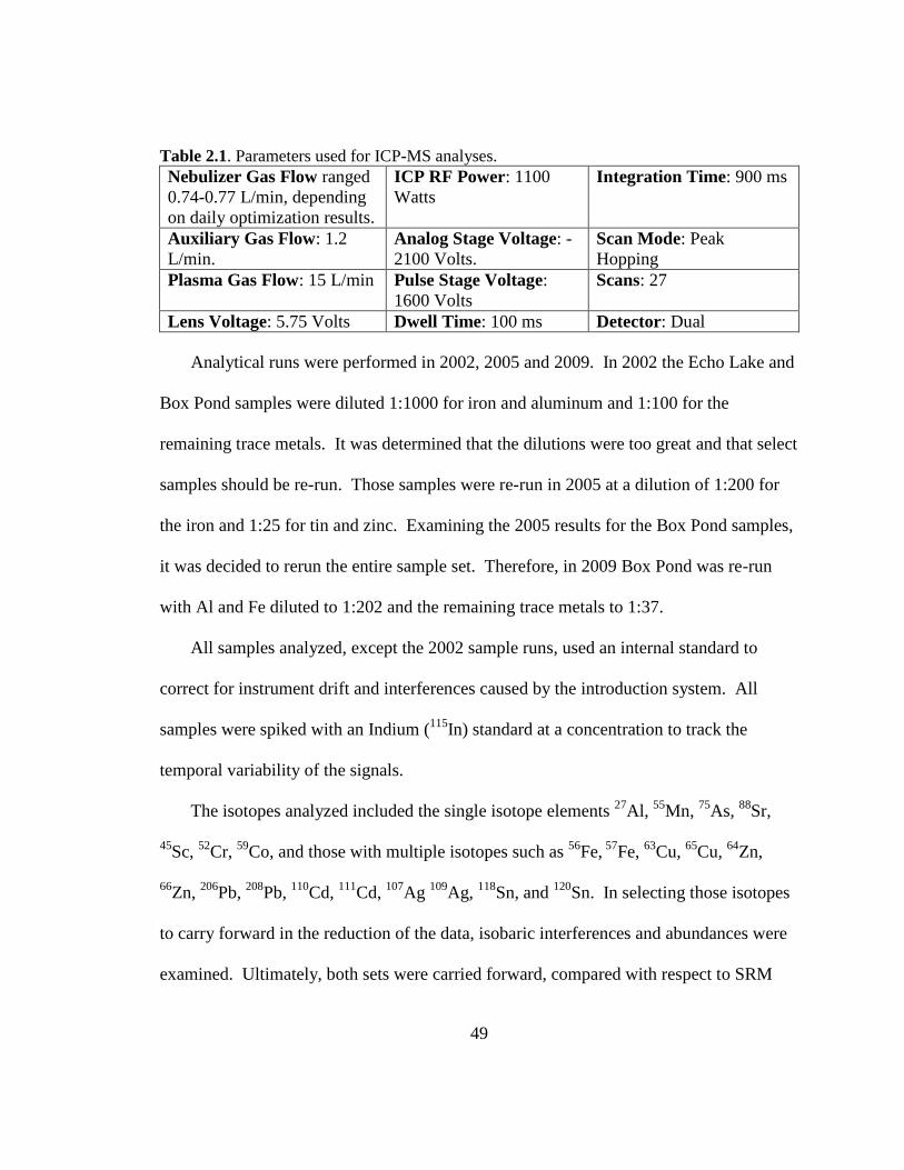
49

Table 2.1. Parameters used for ICP-MS analyses.

Nebulizer Gas Flow ranged

0.74-0.77 L/min, depending

on daily optimization results.

ICP RF Power: 1100

Watts

Integration Time: 900 ms

Auxiliary Gas Flow: 1.2

L/min.

Analog Stage Voltage: -

2100 Volts.

Scan Mode: Peak

Hopping

Plasma Gas Flow: 15 L/min Pulse Stage Voltage:

1600 Volts

Scans: 27

Lens Voltage: 5.75 Volts Dwell Time: 100 ms Detector: Dual

Analytical runs were performed in 2002, 2005 and 2009. In 2002 the Echo Lake and

Box Pond samples were diluted 1:1000 for iron and aluminum and 1:100 for the

remaining trace metals. It was determined that the dilutions were too great and that select

samples should be re-run. Those samples were re-run in 2005 at a dilution of 1:200 for

the iron and 1:25 for tin and zinc. Examining the 2005 results for the Box Pond samples,

it was decided to rerun the entire sample set. Therefore, in 2009 Box Pond was re-run

with Al and Fe diluted to 1:202 and the remaining trace metals to 1:37.

All samples analyzed, except the 2002 sample runs, used an internal standard to

correct for instrument drift and interferences caused by the introduction system. All

samples were spiked with an Indium (115

In) standard at a concentration to track the

temporal variability of the signals.

The isotopes analyzed included the single isotope elements 27

Al, 55

Mn, 75

As, 88

Sr,

45Sc,

52Cr,

59Co, and those with multiple isotopes such as

56Fe,

57Fe,

63Cu,

65Cu,

64Zn,

66Zn,

206Pb,

208Pb,

110Cd,

111Cd,

107Ag

109Ag,

118Sn, and

120Sn. In selecting those isotopes

to carry forward in the reduction of the data, isobaric interferences and abundances were

examined. Ultimately, both sets were carried forward, compared with respect to SRM

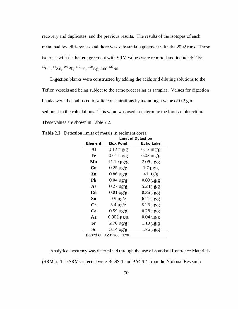
50

recovery and duplicates, and the previous results. The results of the isotopes of each

metal had few differences and there was substantial agreement with the 2002 runs. Those

isotopes with the better agreement with SRM values were reported and included: 57

Fe,

65Cu,

64Zn,

206Pb,

110Cd,

109Ag, and

120Sn.

Digestion blanks were constructed by adding the acids and diluting solutions to the

Teflon vessels and being subject to the same processing as samples. Values for digestion

blanks were then adjusted to solid concentrations by assuming a value of 0.2 g of

sediment in the calculations. This value was used to determine the limits of detection.

These values are shown in Table 2.2.

Table 2.2. Detection limits of metals in sediment cores. Limit of Detection

Element Box Pond Echo Lake

Al 0.12 mg/g 0.12 mg/g

Fe 0.01 mg/g 0.03 mg/g

Mn 11.10 µg/g 2.06 µg/g

Cu 0.25 µg/g 1.7 µg/g

Zn 0.86 µg/g 41 µg/g

Pb 0.04 µg/g 0.80 µg/g

As 0.27 µg/g 5.23 µg/g

Cd 0.01 µg/g 0.36 µg/g

Sn 0.9 µg/g 6.21 µg/g

Cr 5.4 µg/g 5.26 µg/g

Co 0.59 µg/g 0.28 µg/g

Ag 0.002 µg/g 0.04 µg/g

Sr 2.76 µg/g 1.13 µg/g

Sc 3.14 µg/g 1.76 µg/g

Based on 0.2 g sediment

Analytical accuracy was determined through the use of Standard Reference Materials

(SRMs). The SRMs selected were BCSS-1 and PACS-1 from the National Research

51

Council of Canada. BCSS-1 is estuarine sediment from the Gulf of St. Lawrence while

PACS-1 is harbor sediment from Esquimalt Harbor, British Columbia. The primary

difference in the two SRM is that metal concentrations in the PACS-1 sediments were

generally higher. Therefore, two ranges would be supplied to cover the range of values

anticipated for Box Pond (high concentrations) and Echo Lake (low concentrations). A

summary of the SRM recoveries for runs of each sediment core is provided in Table 2.3.

52

Table 2.3. Summary of Standard Reference Material recoveries. Echo Lake and Box

Pond analytical runs.

Element

Core

Location

Maximum

Conc.

Average

Conc.

BCSS-1

certified

value

%

Agree

PACS-1 certified

value % Agree

Al Echo Lake 76 mg/mL 37 mg/mL

63 mg/mL 97.50% 65

mg/mL

102.44%

Box Pond 68 mg/mL 48 mg/mL 103.20% 100.20%

Fe Echo Lake 90 mg/mL 24 mg/mL

33 mg/mL 101.39% 49

mg/mL

96.64%

Box Pond 42 mg/mL 25 mg/mL 111.30% 108.70%

Mn Echo Lake 952 µg/mL 436 µg/mL

229 µg/mL 110.70% 470

µg/mL

104.52%

Box Pond 597 µg/mL 345 µg/mL 125.73% 102.08%

Cu Echo Lake 70 µg/mL 24 µg/mL

18.5 µg/mL 110.50% 452

µg/mL

100.60%


Zn Echo Lake 279 µg/mL 119 µg/mL

119 µg/mL 109.87% 824

µg/mL

102.52%


Pb Echo Lake 134 µg/mL 76 µg/mL

22.7 µg/mL 113.03% 404

µg/mL

103.96%


As Echo Lake 19 µg/mL 10 µg/mL

11.1 µg/mL 105.99% 211

µg/mL

91.23%


Cr Echo Lake 58 µg/mL 29 µg/mL

123 µg/mL 93.52% 113

µg/mL

91.02%


Cd Echo Lake 1.43 µg/mL 0.53 µg/mL

0.25 µg/mL 97.20% 2.38

µg/mL

104.07%

Box Pond 5.3 µg/mL 2 µg/mL 104.59% 110.37%

Co Echo Lake 19.1 µg/mL 5.9 µg/mL

11.4 µg/mL 110.14% 17.5

µg/mL

112.32%

Box Pond 14.2 µg/mL 6 µg/mL 105.08% 92.25%

Sn Echo Lake 15.6 µg/mL 2.9 µg/mL

1.85 µg/mL 61.30% 41.1

µg/mL

110.39%


Ag, Sc &

Sr

No SRM were available for these elements. They were run to gauge the crustal input (Sc and

Sr) and anthropogenic activities (Ag) qualitatively.

A summary of isotopes analyzed, limits of detection, replicate recoveries and SRM

recoveries is presented in Tables II-1 and II-3 in Appendix II. The SRM recoveries,

limits of detection, and blanks were examined to determine suitability for discussion in

subsequent chapters. SRM recovery was acceptable (within 10% of the accepted value)

for Al, Fe, Cu, As, Co, and Cd. The metals Mn, Zn, Pb, and Cr were within 25% of their

accepted values for the BCSS-1 SRM in Box Pond sediments. A comparison of the range

of concentrations of Mn, Zn, Pb and Cr in Box Pond sediments with the SRMs, shown in

Table II.2 as well as by the maximum and average concentrations shown for each water

53

body in Table 2.3, demonstrates that the PACS-1 SRM is more appropriate than the

BCSS-1 SRM for these metals. The greatest disagreement was the BCSS-1 SRM for Sn

in Echo Lake. Although the range of concentrations may also make the PACS-1 SRM

more appropriate, caution should be exercised in examining the Echo Lake Sn data. All

quality assurance and quality control measures are reported in Appendix II. Three

elements had no SRM available, Sc, Sr and Ag. Sc and Sr were included in the analysis

to qualitatively support the evaluation of crustal contribution.

2.6 Mercury Analysis via Cold Vapor Atomic Adsorption

For Hg analysis the stock solution was diluted and analyses performed using a

CETAC Model 6000A Mercury analyzer with a detection limit of 1 ng/l in the final

digestate using a method similar to method EPA Method 245.5. Blanks were run at a

frequency of 1 blank to each 10 samples analyzed. Standards were run every five

samples throughout the cold-vapor analytical run. The SRM selected was PACS-1, the

same as used for the metals in the ICP-MS. For both sets of data, Echo Lake and Box

Pond, SRM were < 10% of the certified values, analytical and digestion replicates were

<5% except for the Echo Lake digestion replicates at 25% driven by one value. Table 2.4

summarizes the quality assurance and quality control measures for the Hg analysis, the

details are provided in Appendix II.

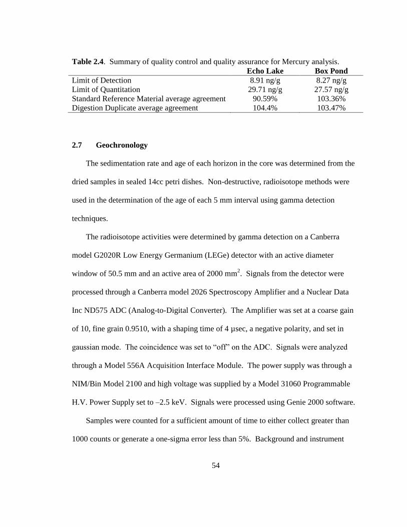
54

Table 2.4. Summary of quality control and quality assurance for Mercury analysis.

Echo Lake Box Pond

Limit of Detection 8.91 ng/g 8.27 ng/g

Limit of Quantitation 29.71 ng/g 27.57 ng/g

Standard Reference Material average agreement 90.59% 103.36%

Digestion Duplicate average agreement 104.4% 103.47%

2.7 Geochronology

The sedimentation rate and age of each horizon in the core was determined from the

dried samples in sealed 14cc petri dishes. Non-destructive, radioisotope methods were

used in the determination of the age of each 5 mm interval using gamma detection

techniques.

The radioisotope activities were determined by gamma detection on a Canberra

model G2020R Low Energy Germanium (LEGe) detector with an active diameter

window of 50.5 mm and an active area of 2000 mm2. Signals from the detector were

processed through a Canberra model 2026 Spectroscopy Amplifier and a Nuclear Data

Inc ND575 ADC (Analog-to-Digital Converter). The Amplifier was set at a coarse gain

of 10, fine grain 0.9510, with a shaping time of 4 µsec, a negative polarity, and set in

gaussian mode. The coincidence was set to “off” on the ADC. Signals were analyzed

through a Model 556A Acquisition Interface Module. The power supply was through a

NIM/Bin Model 2100 and high voltage was supplied by a Model 31060 Programmable

H.V. Power Supply set to –2.5 keV. Signals were processed using Genie 2000 software.

Samples were counted for a sufficient amount of time to either collect greater than

1000 counts or generate a one-sigma error less than 5%. Background and instrument

55

drift were checked after every ten samples and approximately 10% of the samples were

recounted for quality assurance.

Two standards were used to calibrate the detector. These included the 4350b

standard and a standard pitchblende ore. Corrections for geometry and detector

efficiency for the radioisotopes in this research, 210

Pb, 214

Pb, and 137

Cs, were found using

the reference materials and were found to be as shown in Table 2.5.

Table 2.5. Overall efficiencies of the Low-Energy Germanium gamma detector.

Radioisotope γ Energy Efficiency 210

Pb 46 keV 0.5114% 214

Pb 295 keV 0.6835% 137

Cs 662 keV 1.40%

Branching efficiencies were found in the literature and incorporated intrinsically into

the geometry and detector efficiency calculations. Self-absorption was calculated by the

method of Cutshall (Cutshall et al. 1983). After the background, decay and yield

corrections, the results were reported in units of dpm/g and Bq/g dry weight.

Radiometric dating techniques use a variety of models based on an assumed

depositional characteristic to determine the dates of sediment horizons. The two basic

divisions are constant rate and variable rate models.

The Constant Flux:Constant Sedimentation rate model (CF:CS) is a constant rate

model based simply on the slope of the activity plotted against the amount of sediment

deposited. To use this model, the activity is transformed by the natural logarithm and the

amount of sediment can be expressed either in depth in centimeters or cumulative mass.

Typically, the cumulative mass is the better to use as sediments become compacted with

depth and diagenetic changes may alter the density of sediments.

56

The variable rate methods include the Constant Rate of Supply (CRS) and

Constant Initial Concentration (CIC) models. These models assume either the amount of

excess 210

Pb is the same every year irrespective of the amount of sediment deposited

(CRS) or that the amount of sediment and radioisotope vary in a co-dependent fashion

(CIC) (Appleby and Oldfield 1978).

In determining which model to employ for the cores, it was necessary to examine

the amount of watershed versus the amount of surface water present at each location and

character of the depositional area. Ultimately, all the models were used on each sediment

core and the results compared. Appendix III describes the models used and how the dates

were developed from those models. The dates of sediment deposition are plotted against

the metal concentrations in Chapters 3 and 4 to yield a chronological concentration

profile.

57

CHAPTER 3

ECHO LAKE WATERSHED

Abstract

A 43 cm long sediment core was collected from Echo Lake, a protected drinking

water reservoir in Hopkinton, Massachusetts, and sectioned at 5 mm intervals.

Radiometric dating, using gamma spectroscopy and the radioisotopes 210

Pb, 214

Pb, and

137Cs, determined absolute dates of deposition for each interval. Each interval was then

analyzed for TOC and the metals Al, Fe, Mn, Hg, Pb, As, Cd, Cu, Zn, Co, Cr, Sn, Ag, Sr,

and Sc.

Increases in sediment Hg concentrations in the late 19th

and early 20th

century were

determined to perhaps be the result of increased railway traffic within the watershed.

Increases in sediment Pb concentrations in the latter half of the 19th

century were due to

atmospheric sources from outside the watershed. Pb concentrations increased through the

20th

century until 1993 when concentrations began to decrease due to the phase-out of

leaded gasoline under the Clean Air Act of 1970.

Residential development began in the watershed in 1970 altering the physical

character of sedimentation and the lake bottom as well as the metal concentrations in

Echo Lake sediment. The rate of sediment deposition in Echo Lake increased by more

than four times the natural rate of deposition. After 1970 the sediment concentrations of

58

Hg, Pb, Cd, and As began increasing due to atmospheric fallout and storm water runoff,

while an increase in Cu sediment concentration was due to a weed treatment performed in

1990. Because of these increases of sediment concentration, seven metals: Hg, Cd, As,

Cu, Zn, Cr, and Pb, were determined to exceed regulatory guidelines established to assess

potential harm to aquatic life.

3.1 Introduction

Echo Lake is a drinking water reservoir in Hopkinton, Massachusetts. Few lakes in

eastern Massachusetts are unaltered by anthropogenic land use changes, but Echo Lake

has been a protected drinking water reservoir since 1882. For much of its history, the

Echo Lake watershed was unpopulated. Until 1968 there were fewer than 16 homes in

the watershed and less than 5% of the watershed was altered by residential development

or agriculture. After 1970, residential development began on the northern edge of the

watershed, approximately 1 km from the lake. Residential development continued to

expand during the 1980’s and 1990’s, but a protective natural buffer of approximately

500 m has been maintained around the reservoir. When the sediment core was collected

in 1999, residential development had altered 39% of the watershed (Dichter 2005).

Three primary questions were examined with respect to Echo Lake: What are the

natural background concentrations of metals in sediments prior to anthropogenic

alteration? What alteration to the concentration of metals in sediment occurred as a result

of anthropogenic land use changes in the watershed? Have those changes in sediment

metal concentration affected water quality and aquatic life?

59

To answer these questions, a 43 cm deep sediment core was collected from Echo

Lake and sectioned at 5 mm intervals. The date of deposition for each interval was

determined with gamma spectrometry using the radioisotopes 210

Pb, 214

Pb, and Cs137

.

Sediments from each interval were acid-fumed and analyzed in a Perkin-Elmer CHN

analyzer to determine the concentration of TOC. A total microwave acid digestion of

sediments from each interval was performed to obtain suitable stock solutions for metal

analysis. Al, Fe, Mn, Pb, As, Cd, Cu, Zn, Co, Cr, Sn, Ag, Sr, and Sc were analyzed via

ICP-MS, while Hg was analyzed using CVAA. The sample preparation, analytical

methods, quality assurance, and quality controls are discussed in Chapter 2.

3.2 Echo Lake Study Area

3.2.1 Echo Lake Watershed Characteristics

Echo Lake is an impoundment created by a 10 m high, granite dam filled by

groundwater and three small streams in Hopkinton, Massachusetts. Its watershed covers

3.7 km2 of which the lake covers 39 hectares. Echo Lake is the headwaters of the Charles

River and lies at an elevation of 106 m above sea level and 125 km upstream, as the river

runs, from the Charles River dam which separates the river from Boston Harbor and the

Atlantic Ocean.

Echo Lake is approximately 9 m deep at its deepest point when the reservoir is full,

but otherwise has large areas that can become exposed during dry summers. Its average

depth is approximately 2 meters and has an approximate volume, when full, of 8x108 l.

The measured flow of the Charles River as it emerged downstream of the Echo Lake dam

60

in 1996 was 0.014 m3 s

-1 (Wohlers 1998). From evidence gathered during the sediment

core collection it appears that the lake bottom in the area of the deepest point of the

reservoir is thermally stratified during the summer months and no benthic vegetation

exists in the area where the core was collected.

The 500-million year-old Milford Granite underlies Echo Lake and much of south-

central Massachusetts. In this area the Milford Granite is a pale gray color, with small

amounts of biotite and quartz (Zen 1983). The general soil type in the area is the

Chatfield-Hollis, a well-drained glacial soil that is present in sloping terrains. One of the

distinguishing characteristics of this soil is that it is typically underlain by bedrock, just

20 to 40 inches below the surface, making the soil rather poor for farming, woodlands, or

development (Taylor 1998). The watershed of the lake is forested with a mix of pine and

hardwood that range from sapling to mature trees.

At the time of the sediment core collection in 1999 approximately 39% of the Echo

Lake watershed consisted of land used for residential homes with the remaining land

consisting of either forest (51%) or the lake itself (10%) (Dichter 2005). The majority of

the 240 homes in the watershed at the time of sediment core collection were greater than

1 km from Echo Lake. The Echo Lake watershed is shown as the dark-grey shaded area

on Figure 3.1.

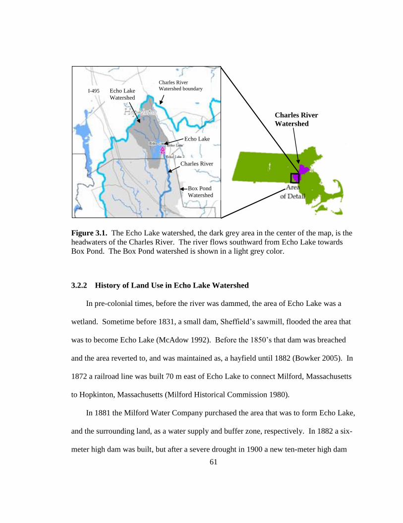
61

Figure 3.1. The Echo Lake watershed, the dark grey area in the center of the map, is the

headwaters of the Charles River. The river flows southward from Echo Lake towards

Box Pond. The Box Pond watershed is shown in a light grey color.

3.2.2 History of Land Use in Echo Lake Watershed

In pre-colonial times, before the river was dammed, the area of Echo Lake was a

wetland. Sometime before 1831, a small dam, Sheffield’s sawmill, flooded the area that

was to become Echo Lake (McAdow 1992). Before the 1850’s that dam was breached

and the area reverted to, and was maintained as, a hayfield until 1882 (Bowker 2005). In

1872 a railroad line was built 70 m east of Echo Lake to connect Milford, Massachusetts

to Hopkinton, Massachusetts (Milford Historical Commission 1980).

In 1881 the Milford Water Company purchased the area that was to form Echo Lake,

and the surrounding land, as a water supply and buffer zone, respectively. In 1882 a six-

meter high dam was built, but after a severe drought in 1900 a new ten-meter high dam

Charles River

Watershed boundary I-495

Echo Lake

Charles River

Watershed

Box Pond

Watershed

Charles River

Echo Lake

Watershed

62

was built on the same location in 1902, which still stands (McAdow 1992). Until 1968

the river ran in a natural, 4 km long channel to the treatment plant in Milford, before

being collected, treated, and then distributed as drinking water. Due to water quality

problems during high river flow events, a pipe was installed at the base of the dam in

1968 to transmit drinking water from Echo Lake, directly to the treatment plant (Papuga

2004). Since the early 1900’s the Milford Water Company has restricted access to the

lake, not allowing any recreational use, and has maintained a natural, forested buffer zone

greater than 500 m, in most places, that is posted to prevent trespassing (Papuga 2004).

3.3 Sediment Core Collection and Description

The Echo Lake sediment core was collected by divers David Shull and Peter Edwards

on August 6th

, 1999 at the deepest point found in the lake. The sediment core location

was determined from a boat using an electronic depth finder and recorded as N42° 11'

32.67" and W71° 30' 31.83" using a compass, triangulating from known landmarks and

then checking against a USGS map. The sediment core collection location was found to

be 6.4 meters deep at the time of collection by electronic depth finder.

The sediment core was collected in mid-summer while the lake level was depressed

approximately 2.5 meters below its usual level. The water column was extremely turbid,

with what appeared to be a bloom of plankton, and the divers disappeared from view at a

depth of less than 1.5 meters. Both divers stated that within a short distance of the

surface the water was completely dark. Although the surface water temperature was

quite warm, 21.1ºC, the divers reported that within 0.5 meter of the lake bottom there was

63

a sharp transition in water temperature to 12.8ºC as shown on a dive watch (Shull 1999).

The diver collected the sediment core by gently pushing the corer in, capping the top,

and then digging under the bottom to put on the bottom cap. The diver reported that there

was additional peat below that which the core intercepted (Shull 1999). The core was

brought to the surface, maintained in an upright position, measured, placed in a bucket,

and surrounded with ice. A second core was collected in an identical manner at that time

as well from an area close to the initial core. The sectioning and processing of the

sediment cores is described in Chapter 2.

A 1-cm layer of water overlying the sediment was collected in 0.5-cm sections

capturing the unconsolidated sediments above the sediment/water interface. Sediment

layers were then collected in 5 mm horizontal intervals. A Munsell Soil Color Chart was

used to characterize the colors of the sections described below (Macbeth 1994) and the

presentation is in the form of “(hue, value/chroma).” The sectioning and character of the

sediment core will be described from the top of the sediment core to the bottom.

From the surface down to 7.5 cm the sediments were black (gley, 2.5/N) and devoid

of structure or organisms. The sediments were loosely consolidated at the surface, and

became more consolidated with depth. From the surface to 3 cm the sediments had an

anaerobic smell but below 3 cm the anaerobic smell gave way to an earthy smell. This

stratum, from the surface to 7.5 cm depth, was termed “Muck.”

The stratum from 7.5 cm to 19.8 cm was black to dark brown (7.5YR, 2.5/1-2), with

many small, fiberous roots, hence it was termed the “Root” stratum. Beginning at 15 cm

a number of small, 2-3 cm diameter gray (gley, 6/5G), clay-like balls were found that

64

persisted until 17.8 cm. The numerous roots indicate that at the time of deposition of

these intervals, the deepest part of Echo Lake was dominated by rooted vegetation.

Figure 3.2 is a photo of typical sediments in the Root stratum.

Figure 3.2. Echo Lake sediments in the root stratum.

The Terrestrial stratum was beneath the Root Zone, from 19.8 cm to 23.8 cm depth,

and contained leaves, twigs, and grasses mixed with the sediment. This material was

deposited when the surrounding area was used as a hayfield in the mid-1800’s (Bowker

2005). The top of this section would appear to have been deposited in 1882 when the

first of two water supply dams were built, trapping sediments that contained the terrestrial

debris.

The Peat stratum contained the lower-most sediment. Peat grows above water and

therefore formed before the area was dammed. The diver reported that substantial peat

underlay the core when he dug through it to place the bottom cap. The presence of a

thick layer of peat indicates that before becoming a lake, this area may have been a

wetland since the glaciers retreated 13,000 years ago. The upper layers of the peat held

65

considerable amounts of sediment within the peat matrix which diminished with depth in

the core. The total length of the sectioned core was 43 cm; however, sectioning stopped

at 35.7 cm when the peat matrix dominated and little sediment was evident.

3.4 Results

The concentrations of Al, Fe, Mn, Pb, As, Cd, Cu, Zn, Co, Cr, Sn, Ag, Sr, Sc, Hg, and

TOC, as well as the absolute date of sediment deposition, were determined for each of the

5mm intervals of the sediment core. The dates assigned to each of the intervals extend

from the sediment/water interface at 1999 to the bottom of the sediment core 35.7 cm,

approximately 1754. The methods and materials used in the analysis of this sediment

core are documented in Chapter 2. The results and quality assurance and quality control

are in Appendix I for TOC, Appendix II for metals, and Appendix III for geochronology.

The stratigraphy and assigned dates of deposition are shown on Table III-2 in Appendix

III.

Figures 3.3 through 3.6 superimpose the strata comprising the sediment core along-

side the concentration profiles and the year of deposition to better relate the sediment

concentration to the environmental conditions during the deposition of that sediment.

The strata present in the sediment core reflect the history of Echo Lake: first as a wetland

(Peat) until 1850’s, then as a field (Terrestrial) until 1882, and lastly as a lake (Roots and

then Muck). The thickness of each stratum shown in the figures is relative to the date of

deposition and not their actual thickness. An unconformity, labeled as a “Disturbed”

66

stratum is shown within the sediment column. This stratum represents an erosion event

or a period of slow deposition and is discussed in Appendix III.

Within the lake sediments, the Disturbed stratum divides the Root stratum into two

units: an “Upper Root” stratum that was deposited from 1969 to 1983, and a “Lower

Root” stratum deposited from 1882 to 1919. During processing of the core there was no

visual indication of the Disturbed stratum. The Disturbed stratum was discovered

through radionuclide dating and, as discussed in Appendix III, was perhaps the result of

bioturbation, erosion, or depositional shading. Although it represents only 2 cm of

sediments, the Disturbed stratum spans 48 years of deposition, from 1920 to 1968.

Within the Disturbed stratum the concentrations are accurate but the dates of deposition

are not believed to be accurate.

Below the Disturbed stratum, the accuracy of the dates derived from the radiometric

dating model, the CF:CS model, was adjusted to account for the Disturbed stratum. The

assumptions inherent in adjusting the CF:CS model prevented assigning uncertainty, but

the modeled dates from 1919 to the bottom of the sediment core are believed to be

accurate. The adjusted CF:CS model accurately dates the change in strata from terrestrial

sediments to lake sediments when the dam was built in 1882. The CF:CS model was

extended to portions of the core that pre-date 1882, based on the assumption that the

depositional rate determined in the sediments between 1919 and 1882 did not change

radically.

Figure 3.3 displays the concentration trends for Al, Sc, Sr, and Co. These metals

have been used for determining the crustal contribution of metals due to erosion from

67

native soils and rock (Feng et al. 2004). Figure 3.4 displays the concentration trends for

Fe, Mn, Cr and TOC. These metals and TOC provide insight into the redox environment

of the sediments (Lovley 1991; Stumm and Morgan 1996). Figure 3.5 displays the

concentration trends of Hg, Pb, As and Cd. These metals have wide-spread

anthropogenic uses and are most commonly associated with toxic effects in aquatic

environments (Stumm and Morgan 1996). Figure 3.6 displays the concentration trends of

Cu, Zn, Sn and Ag. These metals are also commonly used in many anthropogenic

materials (Davis et al. 2001). Despite their common use, these metals may have toxic

properties to aquatic life and affect the overall quality of sediments and surface waters


68

Figure 3.3. Sediment concentration profiles of Al, Sr, Sc and Co.

1750

1775

1800

1825

1850

1875

1900

1925

1950

1975

2000

0 20 40 60 80 100

Ye

ar o

f D

ep

osi

tio

n

a. Echo Lake

Aluminum (mg/g)

Peat

Terre.

Roots Roots

Disturbed

Muck

1750

1775

1800

1825

1850

1875

1900

1925

1950

1975

2000

0 40 80 120 160 200

Ye

ar o

f D

ep

osi

tio

n

b. Echo Lake

Strontium (µg/g)

1750

1775

1800

1825

1850

1875

1900

1925

1950

1975

2000

10 20 30 40 50 60 70

Ye

ar o

f D

ep

osi

tio

n

c. Echo Lake

Scandium (µg/g)

Peat

Terre.

Roots Roots

Disturbed

Muck

1750

1775

1800

1825

1850

1875

1900

1925

1950

1975

2000

0 5 10 15 20

Ye

ar o

f D

ep

osi

tio

n

d. Echo Lake

Cobalt (µg/g)

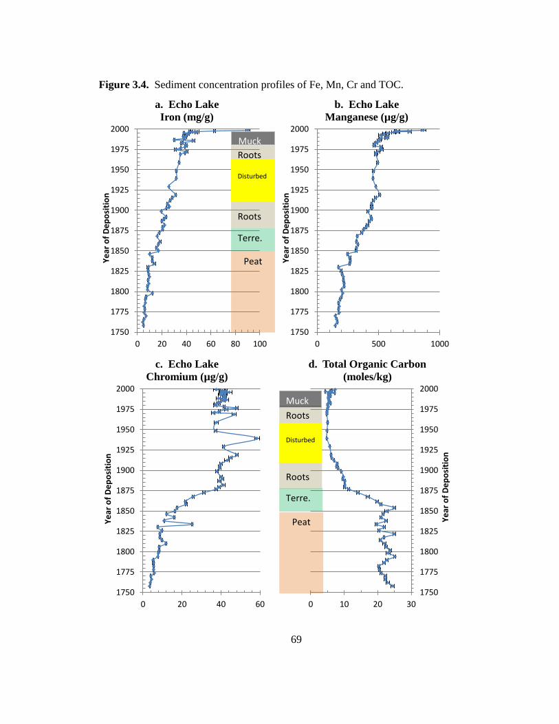
69

Figure 3.4. Sediment concentration profiles of Fe, Mn, Cr and TOC.

1750

1775

1800

1825

1850

1875

1900

1925

1950

1975

2000

0 20 40 60 80 100

Ye

ar o

f D

ep

osi

tio

n

a. Echo Lake

Iron (mg/g)

Peat

Terre.

Roots Roots

Disturbed

Muck

1750

1775

1800

1825

1850

1875

1900

1925

1950

1975

2000

0 500 1000

Ye

ar o

f D

ep

osi

tio

n

b. Echo Lake

Manganese (µg/g)

1750

1775

1800

1825

1850

1875

1900

1925

1950

1975

2000

0 20 40 60

Ye

ar o

f D

ep

osi

tio

n

c. Echo Lake

Chromium (µg/g)

1750

1775

1800

1825

1850

1875

1900

1925

1950

1975

2000

0 10 20 30

Ye

ar o

f D

ep

osi

tio

n

d. Total Organic Carbon

(moles/kg)

Peat

Terre.

Roots Roots

Disturbed

Muck

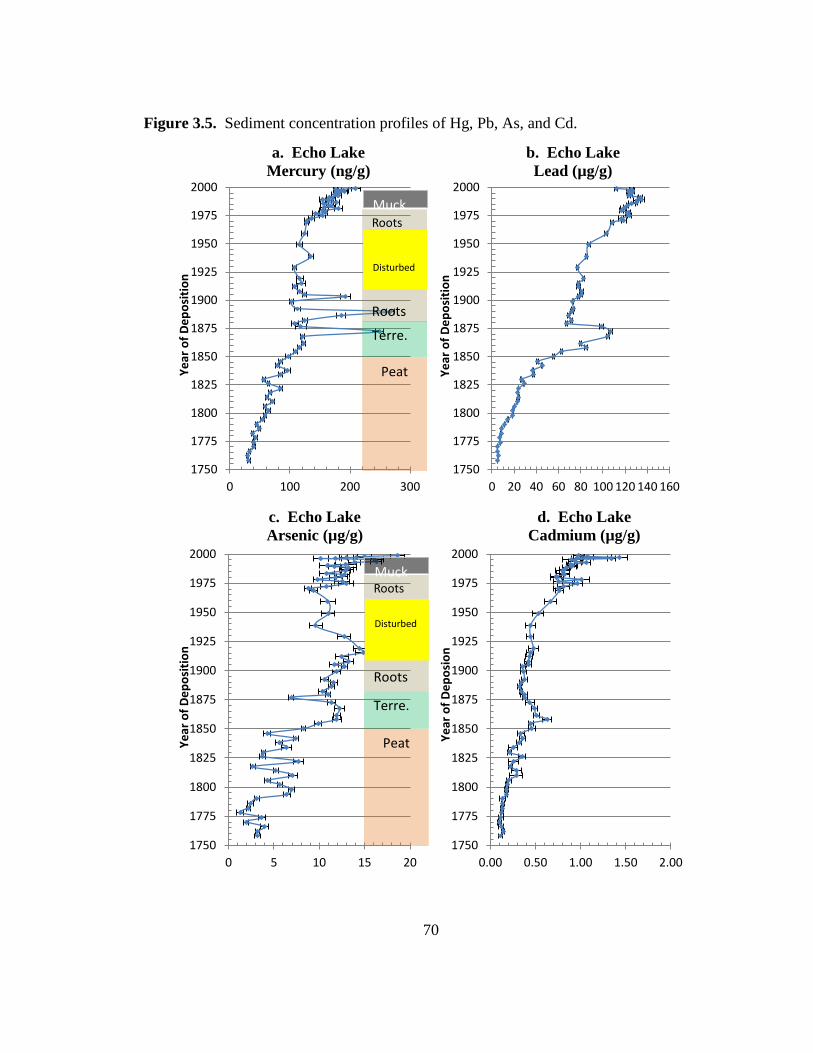
70

Figure 3.5. Sediment concentration profiles of Hg, Pb, As, and Cd.

1750

1775

1800

1825

1850

1875

1900

1925

1950

1975

2000

0 100 200 300

Ye

ar o

f D

ep

osi

tio

n

a. Echo Lake

Mercury (ng/g)

Peat

Terre.

Roots

Roots

Disturbed

Muck

1750

1775

1800

1825

1850

1875

1900

1925

1950

1975

2000

0 20 40 60 80 100 120 140 160

Ye

ar o

f D

ep

osi

tio

n

b. Echo Lake

Lead (µg/g)

1750

1775

1800

1825

1850

1875

1900

1925

1950

1975

2000

0 5 10 15 20

Ye

ar o

f D

ep

osi

tio

n

c. Echo Lake

Arsenic (µg/g)

Peat

Terre.

Roots

Roots

Disturbed

Muck

1750

1775

1800

1825

1850

1875

1900

1925

1950

1975

2000

0.00 0.50 1.00 1.50 2.00

Ye

ar o

f D

ep

osi

on

d. Echo Lake

Cadmium (µg/g)

71

Figure 3.6. Sediment concentration profiles of Cu, Zn, Sn, and Ag.

1750

1775

1800

1825

1850

1875

1900

1925

1950

1975

2000

0 20 40 60 80

Ye

ar o

f D

ep

osi

tio

n

a. Echo Lake

Copper (µg/g)

Peat

Terre.

Roots

Roots

Disturbed

Muck

1750

1775

1800

1825

1850

1875

1900

1925

1950

1975

2000

0 100 200 300

Ye

ar o

f D

ep

osi

tio

n

b. Echo Lake

Zinc (µg/g)

1750

1775

1800

1825

1850

1875

1900

1925

1950

1975

2000

0 5 10 15 20

Ye

ar o

f D

ep

osi

tio

n

c. Echo Lake

Tin (µg/g)

Peat

Terre.

Roots Roots

Disturbed

Muck

1750

1775

1800

1825

1850

1875

1900

1925

1950

1975

2000

0.00 0.50 1.00

Ye

ar o

f D

ep

osi

tio

n

d. Echo Lake

Silver (µg/g)

72

3.5 Discussion

The sediment concentration trends in Figures 3.3 through 3.6, with the exception of

TOC, share a common character: low concentrations in the Peat stratum, increases in

concentration through the Terrestrial stratum, and relatively consistent concentrations in

the overlying lake sediments. This trend is due to the transition from atmospheric

deposition in the Peat stratum to fluvial deposition, where runoff may contribute

additional metals in the lake sediments.

The concentration profiles seen in lake sediments for Al, Sr, Sc, Co, Cr, As, Ag, Zn,

and Sn are generally constant, with no consistent trends. This would indicate that there

was no anthropogenic addition of these metals into the Echo Lake watershed. The

concentration profiles for Hg, Pb, Cd, and Cu reveal anomalies at distinct intervals that

may provide insight into land use changes that have occurred in the Echo Lake

watershed.

Potential sources of metals to the Echo Lake watershed include atmospheric

deposition from natural and industrial sources from the early 1800’s to the present.

Other, more local, sources of metals may include disturbances of the watershed such as

when the railroad line was completed from Milford to Hopkinton in 1872, when the Echo

Lake dam was built in 1882, and when the height of the dam was increased in 1902.

After 1902 little activity occurred in the area until a pipe was installed in the bottom of

the dam in 1968. In 1970 residential subdivision in the watershed began and the road

network serving those homes began to expand.

73

The potential sources of anthropogenic metals from atmospheric fallout include coal-

fired electrical power generators in the mid-west U.S. and industries in and near the City

of Worcester and Millbury, Massachusetts (Wallace et al. 2004). Worcester, 25 km west

of Echo Lake, is noted as having a significant steel manufacturing capability, glass

works, munitions manufacture, and many milling and casting operations beginning early

in the19th

century (Stone 1930). Located 21 km west of Echo Lake in Millbury,

Massachusetts is a waste-to-energy facility that has operated since 1987, incinerating up

to 1.3x106 kg of residential and commercial wastes each day (Massachusetts Department

of Environmental Protection 2011). Industrial emissions and incineration of residential

and commercial wastes can be a significant source of many metals including Pb, Cd and

Hg to the atmosphere (Golomb et al. 1997; Chillrud et al. 1999).

To address the questions posed in Section 3.1, based on an examination of the results

shown in Figures 3.3 through 3.6, the examination of the sediment metal concentration

profiles is divided into four sections:

1. The background conditions that existed before anthropogenic alteration in the

watershed.

2. The anomalies found in the concentration profiles in Hg and Pb that occur

before 1970.

3. The trends and anomalies observed for Hg, Pb, Cd, As, and Cu after

residential subdivision begins in 1970.

4. The potential effects that the concentrations and trends for Hg, Pb, Cd, As

and Cu may have on aquatic life and human health.

74

3.5.1 The Background Contribution of Metals to Sediment in Echo Lake

The contribution of background metals, the portion that results from weathering of

native rocks and soils in the watershed and from atmospheric fallout, must be determined

to ascertain the contribution of metals from other sources. Because the Echo Lake

watershed had few disturbances before 1969, and those after 1969 were from a singular

source, residential development, it was selected as the background sampling location.

In this research two background concentration values were developed: atmospheric

fallout due only to natural conditions before industrial development, and the contribution

of metals to lake sediments after 1882 and before 1919. The natural background

concentrations of metals due to atmospheric fallout were determined by examining

sediments that were dated to be deposited during the period 1762 to 1782 before

industrial expansion in New England. The background conditions between 1882 and

1919 provide a baseline of concentrations when industry was active in New England but

before residential development (Stone 1930; Cronon 1983).

The ideal method to determine background concentrations would be to examine the

concentration of metals in sediments that pre-date anthropogenic alteration. This method

is flawed for Echo Lake because prior to 1831, Echo Lake was a peat bog that had existed

perhaps since the end of the last North American glacial period. The deposition of metals

in a peat bog is different from a lake (Stumm and Morgan 1996; MacKenzie et al. 1998).

Peat bogs lack the fluvial contribution, homogenization, and aerobic environment found

in lakes (MacKenzie et al. 1998; Kalff 2002). The reducing conditions in peat bogs,

created by the abundant organic matter, cause Fe, Mn and many of the trace metals to

75

become soluble, whereas Hg, Pb, Cd, As and Sn have significant tendencies to bind with

sulfur (-SH) and nitrogen (-NH) groups common in organic matter and peat (Stumm and

Morgan 1996). The result is that peat deposits provide a record of the atmospheric

contribution of Hg, Pb, Cd, As, and Sn but that the record of other metals may be

unreliable (MacKenzie et al. 1998). Table 3.1 shows the average concentration and

deposition rate of Hg, Pb, Cd, As and Sn for sediments estimated to have been deposited

during the period 1762 to 1782 when the future coring location was a peat bog and

atmospheric fallout from industry was either minimal or non-existent.

Table 3.1. Average sediment concentration and deposition rates for Hg, Pb, Cd, As, and

Sn from natural atmospheric sources to the sediments in Echo Lake.

Average Sediment

Concentration

Echo Lake 1762 – 1782

Average

Deposition Rate

(g m-2

yr-1

)

Hg 37.1 ± 4.8 ng/g 4.9 x 10-6

Pb 6.4 ± 1.4 µg/g 8.3 x10-4

As 2.7 ± 1.1 µg/g 3.4 x10-4

Cd 0.12 ± 0.01 µg/g 1.6 x10-5

Sn 0.15 ± 0.04 µg/g 2.0 x10-5

Both the average sediment concentration and average deposition rate for each metal

are provided to enable comparison with other research. Research that did not obtain the

dates of deposition cannot develop deposition rates. Deposition rates are derived from

concentrations and the overall delivery of sediment by multiplying the concentration of

each metal by the mass of sediment in a unit area and then dividing by the number of

years each interval represents.

The values in Table 3.1 represent the contribution of volcanic emissions and aeolian

erosion to Echo Lake sediments. The natural atmospheric background Hg sediment

76

concentration determined for Echo Lake in Table 3.1, 4.9 µg m-2

yr-1

, compares well to

other research that found the historic atmospheric deposition of Hg in other New England

lakes before 1850 ranged from 5 to 17 µg m-2

yr-1

(Kamman and Engstrom 2002). The

concentration of Pb in pre-industrial Echo Lake sediments shown in Table 3.1, 6.4 µg g-1

,

agrees with concentrations of pre-industrial Pb in Canadian peat deposits which ranged

from 0.3 to 52.5 µg g-1

(Kylander et al. 2009).

Once the dam was built in1882 and until 1919, the last sediment interval that was

dated with confidence until 1969, there were no disturbances in the Echo Lake watershed

likely to impact the concentration of metals (Bowker 2005). The sediments deposited

after 1882 were formed in a reservoir. These sediments record the contribution of the

natural materials of the watershed and atmospheric fallout from the growing industries in

the area (Stone 1930; Kalff 2002). Table 3.2 provides average concentrations for each

metal in each stratum as shown in Figures 3.3 through 3.6. The background contributions

of metals from natural sources and industrial atmospheric fallout during the period 1882

to 1919 are shown in the row listed as “Lower Root.”

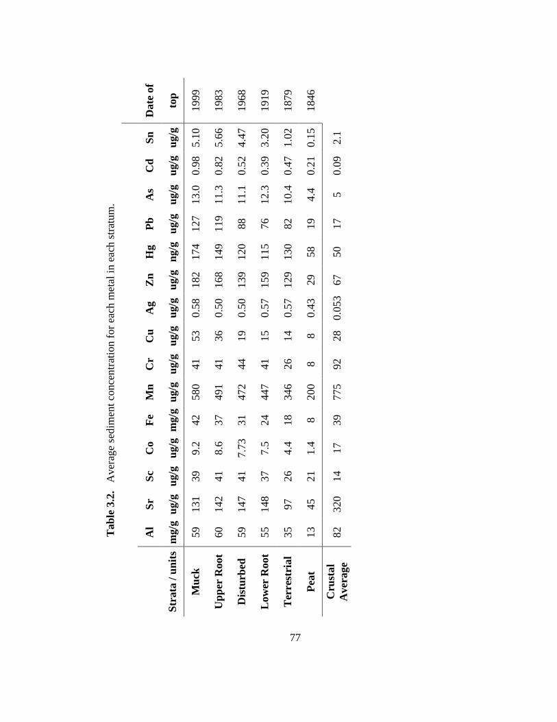
77

Date

of

top

1999

1983

1968

1919

1879

1846

T

ab

le 3

.2. A

ver

age

sedim

ent

conce

ntr

atio

n f

or

each

met

al i

n e

ach s

trat

um

.

Sn

ug/g

5.1

0

5.6

6

4.4

7

3.2

0

1.0

2

0.1

5

2.1

Cd

ug/g

0.9

8

0.8

2

0.5

2

0.3

9

0.4

7

0.2

1

0.0

9

As

ug/g

13.0

11.3

11.1

12.3

10.4

4.4

5

Pb

ug/g

127

119

88

76

82

19

17

Hg

ng/g

174

149

120

115

130

58

50

Zn

ug/g

182

168

139

159

129

29

67

Ag

ug/g

0.5

8

0.5

0

0.5

0

0.5

7

0.5

7

0.4

3

0.0

53

Cu

ug/g

53

36

19

15

14

8

28

Cr

ug/g

41

41

44

41

26

8

92

Mn

ug/g

580

491

472

447

346

200

775

Fe

mg/g

42

37

31

24

18

8

39

Co

ug/g

9.2

8.6

7.7

3

7.5

4.4

1.4

17

Sc

ug/g

39

41

41

37

26

21

14

Sr

ug/g

131

142

147

148

97

45

320

Al

mg/g

59

60

59

55

35

13

82

Str

ata

/ u

nit

s

Mu

ck

Up

per

Root

Dis

turb

ed

Low

er R

oot

Ter

rest

rial

Pea

t

Cru

stal

Aver

age

78

Table 3.2 also provides three useful comparisons. First, it allows a comparison of

each stratum to average crustal concentrations in the literature. Table 3.2 allows a

comparison of the two depositional environments: the wetland peat and the lake

sediments. Lastly, it is an indication of metals with anomalous increases above natural

concentrations indicated by the Lower Root stratum and the crustal averages. These

comparisons were more easily explored by dividing the metals in this research into two

broad groups based on their geochemical behavior and how they move through a

watershed. These groups are the lithophiles and atmophiles (Stumm and Morgan 1996).

The lithophiles move through a watershed primarily by transport in streams in

particulate or dissolved form. The lithophile metals examined in this research include:

Al, Fe, Mn, Sr, Sc, Co, Cr, Cu, Zn, and Ag. In the Echo Lake watershed these metals are

largely derived from the glacial till and the Milford Granite that make up the underlying

geologic materials. As shown in Table 3.2, Al, Sr, Sc, Co, and Cr have relatively

constant, average concentrations in Echo Lake sediments, which represent background

concentrations, from 1882 until the core was collected in 1999. But several other

lithophile metals, Fe, Mn, Ag, Cu and Zn do not share that character and have different

concentration profiles that indicate changes in deposition or chemistry.

Fe and Mn have concentrations that gradually increase in younger sediments with

little variation as shown in Figures 3.4a and 3.4b. Both Fe and Mn are sensitive to

redoximorphic reactions that occur in sediments (Lovley 1991). These redox reactions

cause particulate and mineral forms of Fe and Mn to become soluble and move within the

sediment column, re-precipitating in aerobic environments typically at the sediment/water

79

interface as hydroxides (Stumm and Morgan 1996). The preponderance of organic

matter, especially in the peat, and the presence of a thermocline at the time of the

collection of the Echo Lake sediment core, indicate that such redox reactions are likely.

The potential for re-mobilization of Fe and Mn is reinforced by the observation that

the sediments in the upper 9 cm of the sediment core changed from a black color to a

brick-red color 24 hours after collection and exposure to the air. The reaction that

occurred was either dissolved Fe2+

in pore water, or iron sulfide species in the sediments,

or both, oxidizing after exposure to air during processing and drying of the sediment core.

The concentration profiles for Fe and Mn in Figures 3.4a and 3.4b are perhaps an

expression of the re-distribution of Fe and Mn due to redox reactions and not diagnostic

of deposition due to historic water quality.

Based on the concentration profiles in Figures 3.3 through 3.6, the redistribution of

other metals did not likely occur. The Echo Lake sediments are typical of many

freshwater environments where the sediments have an upper layer, generally less than 1

cm thick, that is aerobic and underlain by an anaerobic layer where respiration takes the

form of sulfate reduction and methanogenesis (Boudreau and Jorgensen 2001). Sulfate

reduction leads to the formation of stable metal sulfide complexes and the order of

stability is generally: Hg>>Cu>Pb>Cd>Zn>Ni, which are more stable than Fe and Mn

sulfide complexes (Stumm and Morgan 1996). Other research performed in Echo Lake

found that the majority of the metals in sediments were bound as sulfides (U.S.

Environmental Protection Agency 1997). The preservation of anomalous concentration

peaks for Hg and Pb indicate that the metal phases associated with sulfides, other than Fe

80

and Mn, are stable and the concentrations are representative of when that sediment was

deposited.

A comparison of the Ag concentrations to the crustal average from the literature

found that the Echo Lake concentration is more than 10 times that average. This anomaly

persists throughout the entire sediment core. The consistent concentration of Ag shown

in Figure 3.6d indicates that natural mineralization is a possible source.

The Milford Granite, which underlies the entire Echo Lake watershed, is listed as

“…granite to granodiorite…” throughout its range, but zones of pegmatite and other

mineralization were also found to exist (Zen 1983). In1881 there was an attempt to mine

gold in the area southwest of Echo Lake which proved uneconomic. Topographic maps

of North Milford note a “Silver Mine Hill” and a road up the hill as “Silver Mine Hill

Road” (U.S. Geological Survey 1895). No information has been found regarding the type

of deposit that the gold works was trying to exploit. These associations indicate that the

above-average concentration of Ag may be the result of a low-grade ore deposit of Ag.

Atmophiles move through the atmosphere as particulates, aerosols, and methylated

forms (Stumm and Morgan 1996). Atmophiles enter the atmosphere via natural

processes such as volcanic emissions as well as industrial discharges to the atmosphere.

The lithophiles are also capable of transport as atmospheric particulates, but the distances

are typically much shorter than that of atmophiles (Stumm and Morgan 1996). The

atmophile metals examined in this research include: Hg, Cd, Pb, As, and Sn.

Because there are no industrial sources in the Echo Lake watershed, atmospheric

fallout of anthropogenic metals such as Hg, Pb, As, Cd and Sn was a regional effect that

81

should be present throughout the Charles River watershed. Therefore, the sediment

concentrations in the Lower Root stratum should provide the background concentrations

and average deposition rate for each of the metals during the period from 1882 to 1919

due to the geology and regional atmospheric fallout. Table 3.3 takes the average values

provided for the Lower Root stratum and develops an average deposition rate.

Table 3.3: Average background concentrations and deposition rates for metals in Echo

Lake sediments from 1882 to 1919.

1882 to 1919

Background

Concentration

Average Deposition Rate

in Echo Lake (g/m2/yr)

Al 55 ± 5 mg/g 9.8 ± 3.3

Sr 148 ± 8 µg/g 0.026 ± 0.008

Sc 37 ± 5.5 µg/g 6.8x10-3

± 2.9x10-3

Co 7.5 ± 1.2 µg/g 1.4x10-3

± 6.0x10-4

Cr 41 ± 3 µg/g 7.4x10-3

± 2.5x10-3

Cu 15 ± 1.8 µg/g 2.8x10-3

± 9.8x10-4

Ag 0.57 ± 0.07 µg/g 1.0x10-4

± 2.7x10-5

Zn 159 ± 31 µg/g 2.8x10-2

± 6.6x10-3

Pb 76 ± 4.5 µg/g 1.4x10-2

± 4.4x10-3

As 12.3 ± 1.4 µg/g 2.2x10-3

± 8.5x10-3

Hg 115 ± 7 ng/g 2.2x10-5

± 6.4x10-5

Cd 0.39 ± 0.05 µg/g 7.1x10-5

± 2.8x10-5

Sn 3.2 ± 1.1 µg/g 6.1x10-4

± 3.8x10-4

Deposition rates in Table 3.3 are corrected for sediment focusing by dividing actual

deposition rates by 2, based on the observed inventories of 210

Pb as discussed in

Appendix III. Sediment focusing is the movement of sediment to deeper locations in a

water body, thereby increasing the apparent rate of sedimentation (Davis and Ford (Jesse)

1982).

82

Two background values for metals in Echo Lake sediment were developed in Tables

3.1 and 3.3. Table 3.1 represents the concentrations and deposition rates for Hg, Pb, As,

Cd and Sn from natural, atmospheric sources prior to industrialization. Table 3.2

provides a comparison of average concentrations for each stratum to determine if

anomalies are present for any of the metals. Table 3.3 presents the background

concentrations for metals in sediments deposited prior to residential subdivision but after

industrialization in the region and therefore were affected by the anthropogenic,

atmospheric fallout.

3.5.2 Mercury and Lead Concentrations in Sediment before 1970

The profiles in Figures 3.3 through 3.6 in sediments deposited after 1882 but before

1970 are generally constant in concentration, hence their use as background values in the

preceding section. The exceptions to constant concentration in this period are the Hg and

Pb concentration profiles which display significant peaks in concentration at discrete

intervals in the sediment column. Hg provided three narrow peaks in the late 19th

and

early 20th

centuries, while Pb had a broad peak that began in 1860 and ended before lake

sediments were deposited in 1882.

Because there was no industry or other land use in the watershed that would have

created these peaks, the source must be anthropogenic atmospheric discharges. Coal has

been determined to be a significant source of Hg, Pb and several other metals to the

atmosphere (Szpunar 1992; Stumm and Morgan 1996). The industrial revolution in the

83

late 19th

century used coal as a primary fuel as did railway transport in eastern

Massachusetts (Sanborn Map Co. October 1910).

The Hg concentration profile in Figure 3.5a shows a steady sediment concentration,

with the exception of three narrow peaks, each spanning 5 to 7 years. The geochronology

dates these three peaks as 1872, 1887 to 1889, and 1903. These dates correspond to

when the railway tracks from Milford to Hopkinton, Massachusetts were laid 70 m east

of Echo Lake in 1872, when the first dam was built in 1882, and when the existing dam

was enlarged in 1902 (Milford Historical Commission 2004). For each of these projects,

the number of rail trips by coal-fired locomotives would have increased tremendously to

deliver men and materials to the work areas. The coincidence of these activities and

deposition times indicate that the likely source of the three Hg peaks in Figure 3.5a is the

result of local burning of coal in locomotives.

Figure 3.5b shows a broad peak of Pb that began in 1861, increased through 1872

and then decreased rapidly beginning in 1877. This peak period encompassed the

American Civil War and ends with the close of the Indian Wars in the western United

States beginning in 1880. Worcester, Massachusetts was a significant munitions

manufacturer and because Pb was the principle component of the projectiles at that time,

that activity may have served as the source of this peak of concentration (Stone 1930).

After 1880, the concentrations of Pb slowly increase through 1919.

Leaded gasoline was introduced in automobiles during the 1920’s to increase octane

and lubricate automobile engine parts (Radford University). The concentrations shown

84

for the years 1929 to 1959 show an increasing trend, but because this period of deposition

may have been disturbed, it is unlikely that the dates of deposition are accurate.

The conclusion is that the increases in Hg and Pb concentration are the result of

atmospheric fallout. The discreet increases in Hg concentration are due to emissions

from locomotives near the lake during periods of construction. The broad increase in Pb

concentrations from the 1860s until the 1880s is due to atmospheric fallout from

munitions manufacturing in Worcester. After 1900 automobiles become an increasing

source of Pb to Echo Lake sediments. The average concentrations and deposition rates

for Hg and Pb, with two of the three Hg peaks removed, were shown in Table 3.3. The

first Hg peak in 1872 pre-dated lake sediments and did not need to be subtracted.

3.5.3 The Supply of Metals to Echo Lake Sediment after 1970

The greatest physical change to the Echo Lake watershed, other than the creation of

the lake in 1882, was the expansion of residential areas beginning in 1970. Before 1970,

the Echo Lake watershed held 16 or fewer homes and it was crossed by only three main

roads that covered a total of 3.7 kilometers. When the sediment core was collected 29

years later there were 240 homes and nearly 12 km of roads. Assuming an average road

width of 9 m, paved surfaces covered approximately 3.3 ha prior to 1970 and 10.3 ha in

1999. The scope and timing of residential land use, compared with the sediment metal

concentration profiles offers insight into contributions of various sources and the effects

of the buffer zone maintained by the Milford Water Supply Company around Echo Lake.

Figure 3.7 shows the extent of land use in the Echo Lake watershed in 1886, 1953, 1980,

85

and 1995, respectively. Each map or photo in Figure 3.7 shows the Echo Lake watershed

with some minor portions of the adjoining watersheds.

86

Figure 3.7. Echo Lake, the majority of its watershed, and the extent of residential land

use for 1886, 1953, 1980 and 1995. Each map or photo is approximately 2.5 km on a

side. The year of the map or photo is shown on the upper left side of each map.

1886 1953

1980 1995

The 1886 map shows a much smaller Echo Lake behind the original, six-meter high

dam built in 1882. In 1902 the original dam was replaced by a ten-meter high dam in the

same location which enlarged the lake to the extent seen in the 1953 map.

87

Residential land use increased from 16 homes in the watershed in 1968 to 240 when

the sediment core was collected. During that period the length of roads increased from

approximately 3,700 m in 1968 to 11,500 m in 1999. The number of homes and road

lengths were estimated from the building permits issued each year in the Echo Lake

watershed (Hopkinton Planning Department 2004). Recent research has used the

percentage of Commercial, Industrial and Transportation network (%CIT) as a measure

of urbanization and impervious surface coverage (Chalmers et al. 2007). This is also a

frequently collected demographic statistic for communities (Commonwealth of

Massachusetts 2012). For comparison to downstream locations, the above estimates of

homes and road length were used to construct a similar statistic for the period of interest,

1970 to 1999, in the Echo Lake watershed.

For the Echo Lake watershed there are no commercial or industrial activities.

Therefore, the %CIT estimate was constructed by multiplying the road lengths at each

interval by an assumed width of 9 m. The resulting values resulted in a calculated %CIT

of 0.9% in 1969 and 2.8% in 1999. These values compare favorably with other nearby

communities with similar distributions (Commonwealth of Massachusetts 2012). For

1999, Hopkinton, Massachusetts, where the Echo Lake watershed lies, was listed as 5.2%

CIT, but the Echo Lake watershed is more rural than the community in general. The

trend of %CIT use developed for the Echo Lake watershed, based on building within the

watershed, is shown in Figure 3.8 (Hopkinton Planning Department 2004).

88

Figure 3.8. Estimate of the amount of impervious surface created by the transportation

network in the Echo Lake watershed, 1969 to 1999.

The increase in the calculated %CIT from 1970 to 1999 was only from 0.9% to

2.8%, respectively. But during this time the overall area altered for residential

development expanded from approximately 5% to 39% of the watershed and the amount

of road network had tripled (Dichter 2005). It was determined that the apparently small

increase in %CIT in the Echo Lake watershed altered Echo Lake sediments both

physically and chemically.

3.5.3.1. Changes in Physical Sedimentation in Echo Lake

The growth of residential land use impacts, as discussed in Chapter 1, impacts

physical characteristics of a watershed. The primary alterations to hydrology cited

included higher storm flows and lower base flows. Perennial streams become more

intermittent and water temperatures rise in receiving water bodies. This translates into

increased scour of stream channels and increased deposition in lakes (Dunne and Leopold

0.0%

0.5%

1.0%

1.5%

2.0%

2.5%

3.0%

1969 1972 1975 1978 1981 1984 1987 1990 1993 1996 1999

Calc

ula

ted

%C

IT

Year

Echo Lake Watershed

89

1978). Erosion from construction sites also contributes to sedimentation (Siver et al.

1996).

The alteration to the upland areas in the Echo Lake watershed is shown in Figure 3.7.

Comparing the 1953 map to the 1980 map, it is apparent that the Charles River View

subdivision in the northern portion of the watershed has altered substantial amounts of

upland areas and filled wetland areas as well. Figure 3.8 shows the growth of this

subdivision which began construction in 1970, expanded in 1975, and again in 1980. By

1980 there were 56 homes built or under construction in the Charles River View

subdivision. Another 55 homes were added during the 1980’s.

The increase in construction increased the amount of sediment delivered to Echo

Lake. Figure 3.9 plots the deposition rate of sediment in the Echo Lake core by mass, the

Mass Accumulation Rate (MAR), compared to the stratigraphy and year of deposition.

90

Figure 3.9. Sedimentation rate of Echo Lake, adjusted for sediment focusing.

Figure 3.9 shows the MAR at the coring location, corrected for sediment focusing.

The MAR in Echo Lake increased from an average of 177 g m-2

yr-1

in sediments that

pre-date 1919, to an average of 417 g m-2

yr-1

in sediment deposited after 1970. The

variability increased in the post-1970 sediments as well, with three periods that exceeded

750 g m-2

yr-1

. The gap from 1919 until 1968 is the Disturbed stratum which was the

result of either an erosion event in 1968 or a period with very low deposition. Those

values were not plotted.

The variations shown in the MAR after 1970 displays a number of interesting

anomalies. A regression of the %CIT developed in Figure 3.8 against the MAR found no

agreement, R2 = 0.02. Focusing on only the post-1970 period, Figure 3.10 plots the

1750

1775

1800

1825

1850

1875

1900

1925

1950

1975

2000

0 500 1000

Ye

ar o

f D

ep

osi

tio

n

Mass Accumulation Rate of

Sediment (g m-2 yr-1)

Peat

Terrestrial

Roots

Disturbed

Roots

Muck

91

deposition rate for sediment from 1970 to 1998 (a), and the flow of the Charles River at

the Dover, MA U.S. Geological Survey (USGS) gauging station (b).

Figure 3.10. Comparison of the Echo Lake sedimentation rate from 1970 to 1998 to the

flow of the Charles River at the USGS gauging station in Dover, Massachusetts.

The average annual flow of the Charles River at the USGS gauging station in Dover,

MA, 30 miles downstream of Echo Lake, was used in Figure 3.10b to approximate

potential runoff in the Echo Lake watershed. Correlation of the sediment mass and

Charles River flow also found little agreement, 0.02, but the peak sediment deposition

years: 1972, 1978, 1984, and 1990, match the peak average annual flow in the Charles

River in Figure 3.10 with the exception of 1997.

The agreement of peak deposition years with peak flows is a measure of the supply

of easily eroded materials from construction sites. The step-wise changes in Figure 3.8

shows construction phases which would present the greatest potential for increases in

sedimentation. The primary increases in %CIT and road length occur when residential

construction occurs in 1971, 1975, 1980, 1984, 1990 and 1995 which correspond with the

increases in MAR shown in Figure 3.10.a.

1969

1974

1979

1984

1989

1994

1999

0 500 1,000 1,500

Ye

ar o

f D

ep

ost

ion

a. Echo Lake

Sedimentation Rate (g m-2yr-1)

Muck

Roots

1969

1974

1979

1984

1989

1994

1999

0 200 400 600 Y

ear

b. Charles River

Average Flow(ft3/s)

92

The sediment column shown in the concentration profiles, Figures 3.3 through 3.6,

documents a profound change in Echo Lake itself. From 1882 to 1983 the bottom of

Echo Lake was dominated by rooted, aquatic plants. In 1984 the rooted plants disappear

and the deposited material transitions to an amorphous black sediment termed “Muck.”

The deposition of Muck continued until the collection of the sediment core. The largest

MAR occurred in 1984, nearly 1 kg m-2

yr-1

adjusted for focusing, more than 5 times the

average deposition rate. The 1984 interval coincides with the extirpation of rooted

vegetation in Echo Lake and a change in the character of deposited sediments to muck. It

was also estimated that from 1983 to 1985 roadways increased from approximately 4200

m to 6000 m and the number of houses increased from 100 to 135 (Hopkinton Planning

Department 2004).

3.5.3.2. Changes in Echo Lake Sediment Chemistry

The concentration profiles shown in Figures 3.3 and 3.4c show little variation in

concentration in lake sediments from 1882 to 1999. This demonstrates that despite the

large increase in MAR noted above, much of the increased sedimentation is due to

erosion of native materials, either erosion from construction sites or scouring of the

channels of the intermittent streams that drain to Echo Lake. After 1970 only Hg, Pb, As,

Cd and Cu display increases in concentration in younger sediments. A closer inspection

of these concentration profiles, focusing on the period after 1969, is provided in Figure

3.11.

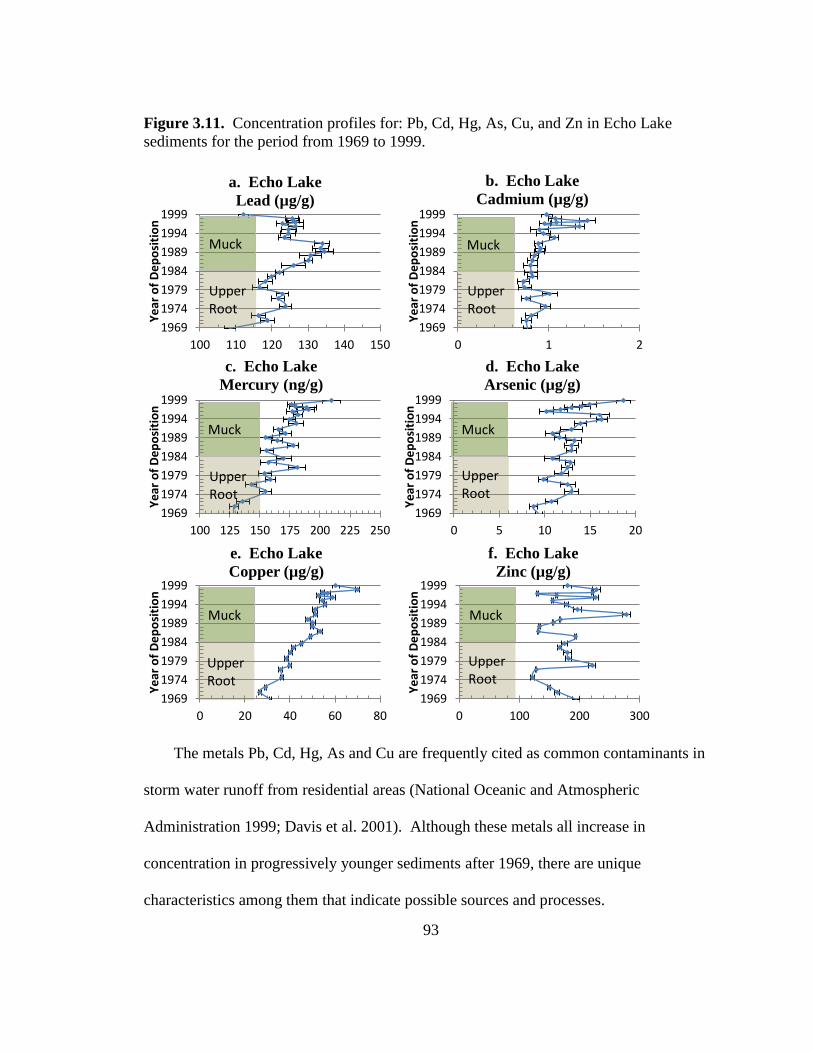
93

Figure 3.11. Concentration profiles for: Pb, Cd, Hg, As, Cu, and Zn in Echo Lake

sediments for the period from 1969 to 1999.

The metals Pb, Cd, Hg, As and Cu are frequently cited as common contaminants in

storm water runoff from residential areas (National Oceanic and Atmospheric

Administration 1999; Davis et al. 2001). Although these metals all increase in

concentration in progressively younger sediments after 1969, there are unique

characteristics among them that indicate possible sources and processes.

1969

1974

1979

1984

1989

1994

1999

100 110 120 130 140 150

Ye

ar o

f D

ep

osi

tio

n

a. Echo Lake

Lead (µg/g)

Upper Root

Muck

1969

1974

1979

1984

1989

1994

1999

0 1 2

Ye

ar o

f D

ep

osi

tio

n

b. Echo Lake

Cadmium (µg/g)

Upper Root

Muck

1969

1974

1979

1984

1989

1994

1999

100 125 150 175 200 225 250

Ye

ar o

f D

ep

osi

tio

n

c. Echo Lake

Mercury (ng/g)

Upper Root

Muck

1969

1974

1979

1984

1989

1994

1999

0 5 10 15 20

Ye

ar o

f D

ep

osi

tio

n

d. Echo Lake

Arsenic (µg/g)

Upper Root

Muck

1969

1974

1979

1984

1989

1994

1999

0 20 40 60 80

Ye

ar o

f D

ep

osi

tio

n

e. Echo Lake

Copper (µg/g)

Upper Root

Muck

1969

1974

1979

1984

1989

1994

1999

0 100 200 300

Ye

ar o

f D

ep

osi

tio

n

f. Echo Lake

Zinc (µg/g)

Upper Root

Muck

94

Pb, Hg, As, and Cd are atmophile metals. Sources of these metals can include

natural and anthropogenic emissions to the atmosphere, as well as common building

materials such as roofing, paint, and treated lumber, in residential areas (Davis et al.

2001). A linear regression of concentrations against both the number of homes and the

length of roadway present in the watershed, represented by %CIT, had strong R2 values

for Hg (0.66) and Cd (0.49), but Pb had a weaker association (R2 = 0.25).

The Pb concentration profile in Figure 3.11 a. is unique. After 1969, Pb

concentrations rise until a peak is reached in 1991 and then concentrations decline in

1993. A primary source of Pb was atmospheric fallout from burning gasoline (Davis et

al. 2001). Tetraethyl lead was a common additive to gasoline beginning in the 1920’s, by

the 1970’s the largest use of Pb was in gasoline. Due to health concerns, the phase out of

leaded gasoline began in 1975 when the first cars that used unleaded gas were produced

(Radford University). In 1996, leaded gas use was banned and through that time,

although leaded gas was available, gradually fewer cars were able to use it (U.S.


The Pb profile in Figure 3.11 a. parallels the characteristics of gasoline use after

1970. In 1979, an economic slump coupled with a disruption of the oil supply, greatly

limited available gasoline, apparently causing a decline in concentration of Pb in

sediments during that time (Schwenk 2001). With improving economic conditions

through the 1980’s gasoline use increased along with concentrations of Pb. These

relationships helped determine the possible sources of the other atmophile metals.

95

To determine the contribution of each source the values for background developed in

Tables 3.1 and 3.3 were examined with respect to the atmophile metal concentrations in

the post-1970 sediments. In 1969, with only 16 homes in the watershed, it was assumed

that there was minimal contribution of these metals from inside the watershed. Table 3.4

compares the concentrations and percentage increases over diagnostic horizons in the

Echo Lake sediment core.

Table 3.4. Sediment concentrations of atmophile metals after 1969.

Pb Hg Cd As Sn

Natural Background (µg/g)a 6 0.037 0.12 2.7 0.15

Industrial Background (µg/g)b 70 0.078 0.27 9.6 3.05

Concentration in 1969 (µg/g) 108 0.128 0.76 9.4 4.78

Increase of Concentrations from

1919 Background to 1969 54% 64% 181% -2% 57%



1969 to 1986 17% 22% 5% 37% 36%



1986 to 1991 6% 6% 11% 0% -9%


Increase of Concentration from

1991 to 1993 -8% 9% 19% 8% 5%

Average Concentration 1996-

1998 (µg/g) 126 0.182 1.18 12.8 5.1

Increase of Concentration from

1993 to 1996-1998 Average 2% 1% 11% -8% -18%

a Values from Table 3.1.

b Values from Table 3.3.

Table 3.4 shows that the atmospheric contribution of industry, compared to its

background for the period 1882 to 1919, had substantially increased by 1969. Much of

96

this increase may be due to the increase of automobile emissions. But after automobile

Pb emissions were virtually eliminated in 1993, Pb had only declined 8%. The increase

of sediment concentration of the other atmophile metals during this period verifies that

the decrease in Pb sediment concentrations is not due to other factors.

This would indicate that either the contribution of Pb from the residential area has

greatly increased or that Pb deposited in watershed soils by past emissions is gradually

being transported to the lake sediments. Although Pb was eliminated in paints in 1977, it

is unlikely that homes would immediately contribute to Echo Lake sediments (U.S.

Consumer Product Safety Commission 1977). By 1977, only 52 homes had been added

to the watershed and all of these were greater than 1 km from Echo Lake. During this

period the calculated %CIT had increased from 0.9% in 1969 to 1.4%.

Table 3.4 also compares the concentrations and the relative changes in atmophiles at

another diagnostic juncture, the creation of a nearby atmospheric source. In 1987 the

Wheelabrator trash to energy facility began operations 21 km west of Echo Lake in

Millbury, Massachusetts. The Wheelabrator facility incinerates approximately 1.3x106

kg of residential and commercial waste from 39 surrounding communities each day

(Massachusetts Department of Environmental Protection 2011). A comparison of

concentrations in 1986 to the 3 year average from 1996 to 1998 finds an increase in Cd

sediment concentrations of 48%. Only Hg increases during this time, by 17%, while the

concentrations of other atmophiles remain stable (Pb) or decrease (As and Sn). It is

notable that during the period 1986 to 1996 the %CIT went from 1.9% to 2.8%, a 48%

increase that parallels the increase in Cd concentration during this time.

97

Cd is geochemically similar to Hg, and occurs in coal in small quantities (Szpunar

1992). A possible source of Cd is the incineration of nickel-cadmium (NiCad) batteries

that may be incorporated into residential wastes. The Wheelabrator facility has more

recently targeted the removal of batteries from its waste stream, primarily to remove Hg

(Wheelabrator 2009). Other research has found that although residential building

materials may contain Cd, they are insignificant sources compared to atmospheric fallout

(Davis et al. 2001). In Figure 3.11b, Cd appears to have no consistent increase in

concentration until 1987 or 1988. Sediment from 1970 to 1987 had an average

concentration of 0.81 ± 0.09 µg/g. Sediment deposited after 1988 had an average

concentration of 1.03 ± 0.19 µg/g, a 20% increase in concentration and a greater than

50% increase in variability over the 1970 to 1987 sediments.

The Echo Lake Hg deposition rate ranged from 10.2 µg m-2

yr-1

in 1969, to 130.4 µg

m-2

yr-1

in 1998, an average deposition rate of 64.2 µg m-2

yr-1

for the 30 year period.

These values are in close agreement with the rate of atmospheric Hg deposition during

the 1990’s in Vermont and New Hampshire lakes which ranged from 21 to 83 ug m-2

yr-1

(Kamman and Engstrom 2002). Deposition rates of Hg as high as 86 ug m-2

yr-1

were

also observed in another lake in eastern Massachusetts (Wallace et al. 2004). The

suspected sources of Hg in the 2004 Wallace study were coal-burning power plants in the

mid-west and nearby medical waste incinerators (Wallace et al. 2004).

The concentration of As in sediments increases over the period from 1970 to 1999,

but concentrations are very low, 9.4 µg/g in 1969 and 15 µg/g in 1999. The thin soils of

the Echo Lake watershed prevented the establishment of orchards and therefore historic

98

agriculture is not a likely source of As (Bowker 2005). The deposition rate of As in Echo

Lake sediments deposited in the early 1970’s was approximately 3x10-3

to 8x10-3

g m-2

yr-1

. This value compares well with average As deposition rates, 2x10-3

µg m-2

yr-1

,

determined in a number of rural areas in the 1970’s (Galloway et al. 1982). The increases

in As sediment concentration parallels that of other atmophile elements in Table 3.4

indicating a potential atmospheric source.

In sediments deposited in the 1990’s the deposition rate for As increases, averaging

0.0046 g m-2

yr-1

which is in agreement with monitoring performed during the same time

period at a station approximately 40 km to the northeast which determined a rate of 0.004

g m-2

yr-1

(Golomb et al. 1997). Monitoring in a rural area in neighboring New

Hampshire had As deposition rates that were as low as 3.2x10-10

g m-2

yr-1

, well below

the rates determined in Echo Lake (Pike and Moran 2001). Because the New Hampshire

watershed lacked nearby industry, the importance of atmospheric sources is apparent.

Therefore, it is likely that the source of As increases in Echo Lake sediments is

atmospheric emissions.

There is a similarity in concentration profiles of Cd, Hg, and As in Figure 3.11b, c

and d, respectively. Correlation analysis of the metal concentrations found some

agreement between the profiles for Hg and Cd (0.52), Hg and Pb (0.49) and Hg and As

(0.56) indicating that these metals share a similar method of transport and incorporation

into the sediments, most likely atmospheric deposition and collection in storm water. Hg

and As share a saw-tooth profile, but the origin of this pattern is not found in the data.

Hg shows a period of 3 years between troughs and peaks, As varies from 1 to 8 years.

99

Correlation with average annual flow or deposition rates found nothing diagnostic. These

differences may indicate that although atmospheric deposition is the likely source of

these metals, different watershed or sedimentation processes affect the concentration

profiles of Hg, Cd and Pb.

Table 3.4 highlights general trends among atmophiles that indicate that atmospheric

fallout is the primary source of these metals to Echo Lake sediments. The less-than-

expected decline of Pb indicates that sorption onto watershed soils and then subsequent

long-term erosion of these soils in storm water is an important contributor to sediment

metal concentrations. The behavior of the other atmophiles in the Echo Lake watershed

may parallel this behavior. This behavior has been demonstrated to occur in other similar

watersheds for Hg and Pb where more than 70% of Hg and 90% of Pb were delivered to

Big Round Top Pond in Rhode Island through runoff from the watershed (Chalmers et al.

2007).

Table 3.4 also demonstrates that environmental regulation has had some effects on

sediment metal concentrations. The clearest example is the 1993 decline of Pb sediment

concentrations due to the Clean Air Act. The emission of Pb was the only metal directly

regulated under the Clean Air Act (CAA), but the slowing of the sediment concentration

increases, especially after 1993, evident in Table 3.4 indicate that regulating the particle

size may be reducing the concentrations of atmophile metals in sediments.

Cu is the only lithophile metal to show a consistent increase in sediment metal

concentration (Davis et al. 2001). The Zn concentration profile is included in Figure 3.11

f. because Zn is commonly found associated with Cu in storm water and overall average

100

concentrations shown in Table 3.2 indicate an increase in concentration in younger

sediments (Davis et al. 2001).

Cu is present in building materials and may also be added to storm water by abrasion

from automobile brakes (Stead-Dexter and Ward 2004). Zn, a lithophile like Cu, is a

significant constituent of residential building materials such as galvanized metal and

roofing and a common component in automobile tires. It is typically present in sediment

affected by storm water runoff and commonly associated with Cu (Davis et al. 2001).

Table 1.2 in Chapter 1 showed that the primary sources of Cu in the Maryland watershed

was automobile brakes (47%) and exterior paint and materials on house siding (22%).

The primary sources for Zn included house siding and galvanized materials (59%), and

automobile tire wear (25%). The anthropogenic contribution of Cu and Zn to those

sediments from the Maryland watershed was 3.8x10-3

and 6.5x10-2

g m-2

yr-1

,

respectively (Davis et al. 2001).

The Maryland watershed had deposition rates of Zn more than an order of magnitude

greater than Cu mirroring results in other research (Chalmers et al. 2007). Table 3.2 does

show an increase in Zn. An average of Zn sediment concentrations for the periods 1969

to 1975 and 1996 to 1998 found an increase in concentration from 157 to 194 µg/g, a

23% increase, while the %CIT increased by greater than 200%. The lack of a definitive

increase for Zn comparable to Cu as shown in Figures 3.6a and b and 3.11e and f,

indicates that building materials and storm water runoff are not primary sources of Cu to

Echo Lake. A regression of Cu and Zn yielded a contradictory result. Although the

101

sediment concentration of Cu agreed well with the %CIT (R2=0.82), Zn sediment

concentrations found no relationship (R2=0.10).

The deposition rate of Cu and Zn in Echo Lake sediments during the 1990’s was

1.9x10-2

and 7.4x10-2

g m-2

yr-1

, respectively. Although the Zn sediment deposition rate

in Echo Lake was similar to that of the Maryland research, Cu was greatly enriched. The

concentration profiles for Cu and Zn were dissimilar as well. Figure 3.12e and f,

respectively show that while Cu increases consistently after 1970, Zn has no discernable

trend. Cu clearly has another source other than storm water runoff.

It was discovered that in 1990 Echo Lake had been treated with an unknown amount

of copper sulfate pentahydrate (CuSO4∙5H2O) to treat a noxious bloom of vegetation

(Papuga 2004). The weed growth may have been due to the runoff of nutrients from

residential areas. In the previous section the amount of sediment supplied to the lake

bottom was shown to have increased dramatically after 1969, and perhaps was

responsible for the extermination of rooted aquatic benthic plants in 1984.

Typical treatments for floating aquatic plants in drinking water reservoirs attempt to

attain a concentration of 0.5 mg/l CuSO4 over a target area of the lake surface area to

avoid a massive kill that would increase biological oxygen demand (Aqua Doc Lake &

Pond Management 2009). Assuming that 10 hectares of Echo Lake, a quarter of the lake

surface, was treated to a depth of 1 meter to attain a 0.5 mg/l dose approximately 20,000

g of Cu would be required. During treatment, the active Cu is incorporated by the plant.

The plant then dies and is conveyed to sediments with the Cu.

102

If the 20 kg of soluble Cu was distributed through the post-1969 sediment column the

total mass of Cu in those sediments would be 0.051 g m-2

. Subtracting that amount of Cu

from the total inventory of Cu in post-1970 sediments, 0.12 g m-2

, yields a difference of

0.07 g m-2

over 30 years or an average Cu deposition rate of 2.3 x 10-3

g m-2

yr-1

. This

compares well with the Maryland site value of 3.8 x 10-3

g m-2

yr-1

(Davis et al. 2001).

The increasing concentration trend shown by Cu in Figure 3.11e shows the trend

beginning in 1971. However, the first and only treatment with copper sulfate was in

1990 (Papuga 2004). Because the copper sulfate is in soluble form when applied, it

penetrated the sediments and was sorbed to the underlying sediments at the

aerobic/anaerobic interface. When the copper sulfate was applied in 1990, the 1971

horizon was only 6.5 cm below the sediment surface. A peak of concentration appears in

the 1987 horizon, which in 1990 was only 1.5 cm from the surface. Interestingly, the

typical thickness of aerobic layers in sediment are from 0.5 to 2 cm in depth (DiToro

2001). Diffusion and travel through pore water since that time has allowed the Cu to be

incorporated in newly deposited sediments as they were added. An increase in sediment

concentrations due to copper sulfate addition has been observed in other areas (Serdar

1995).

Approximately 88% of the Cu increase in post-1970 sediments appears to have been

added through weed treatment. The remainder is most likely due to storm water runoff

from roadways and building. The lack of a clear trend in Zn concentrations, yet an

overall increase in concentration through time indicates that although storm water

103

supplies these metals from road runoff, watershed processes affect the sediment

concentrations of Cu and Zn.

3.5.4 The Potential Effect of Metals in Echo Lake Sediment on Biota

The increase in concentration of Hg, As, Pb, Cd, and Cu in sediments during the

period from 1970 to 1999, raises the prospect of possible environmental harm. The toxic

properties of Hg, As, Pb, Cd, and Cu in sediments are well known (U.S. Environmental

Protection Agency 1997). The significance of ERL and ERM values was discussed in

Chapter 1. Table 3.5 displays the metals investigated in this research with the established

ERL and ERM values as well as the crustal averages. These values are offered for

comparison to the background concentration (from Table 3.3) that provide an indication

of what would be expected from atmospheric fallout, and the average concentrations in

the upper 7.5 cm of sediments that have been deposited since 1984.

104

Table 3.5. Comparison of sediment metals concentrations in Echo Lake to crustal

averages and regulatory guidelines. The bold values exceed the ERL or ERM established

for sediments.

Echo Lake Sediments

Average a

Crustal

Concentration

(µg/g)

Background

Concentration

(µg/g)

Average

Concentration

1984 to 1998

(µg/g)

ERLb

(µg/g)

ERMb

(µg/g)

Cr 92 41 ± 3 41.2 ± 1.5 39 270

Hg 50 0.115 ± 0.007 0.174 ± 0.001 0.180c 1.060

c

Pb 17 76 ± 4.5 127 ± 4.1 55 99

As 5 12.3 ± 1.4 13.1 ± 1.8 13 50

Cd 0.09 0.39 ± 0.05 0.98 ± 0.19 0.7 3.9

Cu 28 15 ± 1.8 53 ± 5.8 41 190

Zn 67 159 ± 31 182 ± 43 110 550 a (Rudnick and Gao 2003),

b (Ingersoll et al. 1996),

c (U.S. Department of Commerce 2012).

Table 3.5 demonstrates that several metals exceed regulatory guidelines. Pb exceeds

the ERM, and Cr, As, Cd, Cu and Zn exceed the ERL in the upper 7.5 cm of sediment

(1984 to 1999). The trend in Hg concentration is increasing and the 1999 horizon

exceeded the ERL, 209 µg/g. The sediment concentration trends for Hg, As, Cd, and Cu

appear to be increasing. Although Pb is not increasing, the average concentration of Pb

in the core after 1993 is 125 ug/g, still well above the ERM of 99 ug/g. Cu may continue

to diffuse from the sediments and, providing there are no further weed treatments, may

decrease in concentration in the future.

With respect to Hg, Cd and As exceeding ERM values, regressing the %CIT against

the concentration found that greater than 1500 additional homes would need to be built in

the watershed to exceed the ERM for any of the other metals. Buildout for the Echo Lake

105

watershed is unlikely to exceed 500 homes, based on the amount of surrounding

developed land and the zoning for the area (Hopkinton Planning Department 2004).

Although the concentration of Pb exceeds the ERM and Hg, Cd, Cu, Zn, Cr and As

exceed the ERL, other research has examined Echo Lake sediments and determined that

most of the metals are bound as sulfides and therefore unlikely to be bioavailable and

cause toxicity (U.S. Environmental Protection Agency 1997). Yet, the potential for

resuspension of these sediments and deposition in other environments may pose a risk to

aquatic organisms (Simpson et al. 1998; Rogers et al. 2002).

3.6 Conclusions

This research determined the background concentrations of selected metals in Echo

Lake sediments during two periods: the natural, atmospheric deposition of Hg, Pb, As,

Cd and Sn before industry was established in the late 18th

century, and the concentrations

of metals in lake sediments between 1882 and 1919. Anthropogenic impacts to Echo

Lake sediments prior to 1919 were found for Hg and Pb. Narrow peaks of Hg

concentration were probably the result of increased local railroad traffic during three

distinct intervals. A broader peak of Pb was delivered through atmospheric deposition

likely due to discharges from industrial sources in Worcester, MA, approximately 25 km

to the west.

Despite a 500 m protected buffer zone, Echo Lake sediments have been impacted

both physically and chemically after residential land use began in 1970. Erosion from

construction sites nearly 1 km from the lake increased the mass accumulation rate of

106

sediment and the concentrations of Hg, Pb, Cd, As, Cu, and Zn. Runoff, perhaps from

residential areas, also required that the lake be treated with Cu to address nuisance

vegetation, causing Cu to exceed regulatory guidelines in Echo Lake. Atmospheric

fallout and the increase of impervious area was the likely, primary source of the increase

in concentration of Hg, Pb, Cd, and As. Regulatory guidelines for aquatic life are

exceeded for Pb, As, Cu, Cr and Zn which, except for Pb, have an increasing

concentration trend. Although Hg did exceed the regulatory guideline in 1999 and the

trend of concentration indicates that it will continue to exceed that standard.

This research found that changes in land use affected the concentrations of metals in

sediments by introducing additional allochthonous metals through the atmosphere and

that the residence time of all metals in the watershed was altered by the collection and

conveyance of metals through storm water. The metals that were formerly retained in

soils of the watershed are being transferred more quickly to the river sediments, but those

metals are retained behind the Echo Lake dam rather than being conveyed to the ocean.

The sediment metals may be a future source of impairment to the environment either

through re-suspension or diffusion.

107

CHAPTER 4

BOX POND WATERSHED

Abstract

A sediment core collected from Box Pond, in Bellingham, Massachusetts, contained

metals from residential and industrial sources. Radiometric dating of the sediment core

using 210

Pb, 214

Pb, and 137

Cs revealed that the sediments spanned the time period from

2000 at the top of the core, to 1905 at the bottom of the core. Industrial sources such as

paint manufacturing contributed Cr, Hg, Pb, Cd, Zn, Cu and Sn, and glass and mirror

manufacturing most likely contributed As and Ag. The concentration of these metals

from industrial sources declined after 1970 due to either economic conditions or

increased environmental awareness. As the contribution of metals to sediments from

industry declined after 1970, other sources, including population, may have contributed

additional metals such as Cu and Ag causing concentrations to either continue increasing

or remain close to their peak industrial concentration. The Milford Sewage Treatment

Works may have also altered sediment metal concentrations in Box Pond during

expansions and other work. High concentrations of metals in historic sediments upstream

of Box Pond may have been re-suspended in 1987 after expansion of the Sewage

Treatment Works. Continuing high concentrations of metals in sediments are likely due

to the re-suspension and deposition of sediments and soils containing high concentrations

108

of metals. The metal concentrations for Cu, Hg, Pb, Cr, Cd, Zn and Sn in the Box Pond

sediments exceed regulatory guidelines, indicating that these sediments may adversely

affect aquatic life. A means of quantifying the flux of anthropogenic metals into the

watershed and the residence time of those metals is needed to protect and restore the

Charles River.

4.1. Introduction

The Charles River traverses a complex geologic terrain, has varied anthropogenic

atmospheric fallout sources along its length, and has an industrial history of nearly 400

years. But the upper watershed of the Charles River, the Box Pond watershed, provides a

unique opportunity to characterize the behavior of metals in sediments.

The Box Pond watershed contains several different land uses, has a common geology,

and is relatively small which minimizes differences in atmospheric fallout. Sediment

cores collected in two impoundments of the Charles River contained anthropogenic

metals that reveal the effects of land use. Echo Lake is the headwaters of the Charles

River and a sub-watershed of the Box Pond watershed. The sediment core taken from

Echo Lake served to define the background contribution of metals. Only 14 km

downstream of Echo Lake, a sediment core was taken from Box Pond in Bellingham,

Massachusetts to determine the effects of more than 150 years of industry and changing

land use. The metal concentrations in the dated sediment core taken from Box Pond were

contrasted against those of Echo Lake to determine the changes in concentration as

109

compared to changes in land use and other anthropogenic factors such as environmental

regulations.

A comparison of the concentrations of metals in sediments in Box Pond with the

concentrations of the metals deposited at the same time in the background sediment core

collected at Echo Lake facilitated the examination of three questions in this research:

1. What is the anthropogenic contribution to sediment metal concentrations in

the Box Pond sediments from various industrial and urban sources?

2. What has been the effect of environmental regulations on metal concentrations

in sediments?

3. What are the potential effects of those sediment metals on aquatic organisms

in Box Pond?

These questions were addressed by collecting a sediment core from Box Pond and

sectioning it at 5 mm horizontal intervals. The date of deposition of each interval was

determined by gamma detection of 210

Pb, 214

Pb, and 137

Cs. Total organic carbon (TOC)

was determined for each interval by collecting a subsample from each interval and acid

fuming the sediment to remove carbonate minerals. Metal concentrations were

determined from stock solutions prepared from total acid microwave digestion of

additional subsamples.

The microwave digestion method used aqua regia, hydrofluoric acid, and boric acid to

completely digest the subsample and produce a stock solution. Mercury (Hg)

concentrations were determined using cold vapor atomic adsorption (CVAA) of aliquots

of stock solution. The metals aluminum (Al), iron (Fe), manganese (Mn), chromium

(Cr), Cobalt (Co), lead (Pb), cadmium (Cd), arsenic (As), tin (Sn), copper (Cu), zinc (Zn),

110

strontium (Sr), scandium (Sc) and silver (Ag) were determined for each interval using an

Inductively Coupled Plasma Mass Spectrometer (ICP-MS). The analytical methods,

quality assurance, and quality controls are discussed in Chapter 2.

4.2. The Box Pond Study Area

The total area of the Box Pond watershed is 38 km2, approximately 5% of the 767

km2 Charles River watershed. The Echo Lake sub-watershed covers 3.7 km

2,

approximately 10% of the Box Pond watershed. The span of the Box Pond watershed,

including that of Echo Lake’s, is approximately 14 km, north to south, and 8 km, east to

west (Dichter 2005). The small size of the Box Pond watershed increases the probability

that the contribution of anthropogenic atmospheric fallout is more likely to be

homogeneous.

The watersheds of Box Pond and Echo Lake share a common geology. The Milford

Granite underlies both watersheds minimizing the differences in autochthonous metals

expected in stream sediments at either sediment core location. The Milford Granite is a

pale grey biotite quartz granite that underlies a large portion of central Massachusetts

(Zen 1983).

The Box Pond watershed is shown as two, gray-shaded areas, light and dark, on

Figure 4.1. The darker shaded area is a sub-watershed of Box Pond, that of Echo Lake,

the headwaters of the Charles River, where the background core was collected. The

remainder of the Box Pond watershed, downstream of Echo Lake, is shown in a lighter

shade of grey.

111

Figure 4.1. The Box Pond watershed, in light grey, also contains the Echo Lake

watershed, shown in dark grey.

Box Pond

Echo Lake

112

A significant portion of the water in Echo Lake is sent southward through a pipe for

distribution as potable water use in Milford, Massachusetts. The small amount of water

that escapes Echo Lake forms the Charles River at the base of the dam and flows

southward towards Milford through mostly forested terrain that contains narrow,

bordering riparian wetlands. Approximately 2.6 km south of Echo Lake, the Charles

River flows beneath Interstate Highway 495 and enters Milford Pond. Milford Pond is

bordered on the northern bank by a large residential area, on the eastern bank by a closed

municipal landfill that is now a park, and on the western bank by several industries. The

Charles River exits Milford Pond to the south and enters a large urban area, where it is

heavily channelized and, in some portions, contained in underground pipes.

Milford became a major manufacturing center in the mid-1800’s. The industries

were located along the Charles River, in particular Milford Pond. The larger industries

initially included granite quarries and stone works, as well as shoe manufacturing and

woolen mills. In the early 20th

century, industries such as paint manufacturing,

electronics, metal works, and glass and mirror manufacture came to the area. Milford

also served as a transportation hub with many coal-burning trains operating between

Providence, Rhode Island and Worcester, Massachusetts until at least 1910 (Milford

Historical Commission 1980). As of 2001, Milford was an urban city of 25,000 with

residential and commercial sections surrounding the river and industry remaining

clustered near the west bank of the Charles River and Milford Pond.

The river emerges from Milford and flows through an area of light residential

development and forest. Approximately 2 km south of Milford and 4 km upstream of

113

Box Pond, the Milford Sewage Treatment Works, a publically-owned treatment works

(POTW) discharges the water originally taken from Echo Lake for use as potable water,

back to the river. The river continues to flow southward in a narrow channel, past a

ruined dam near what is now Hartford Avenue, where a woolen mill burnt to the ground

in the 1860’s and was not re-built.

Box Pond is a narrow, shallow impoundment created by a dam near Depot Street in

Bellingham, Massachusetts. Box Pond is approximately 1.3 km long and is no more than

100 m wide at its widest point. Its depth is quite shallow, and based on a number of short

surveys with a fish finder, no more than 2 m at the deepest with an average depth of

approximately1.5 m. As the Charles River flows eastward from the dam at Box Pond it is

still a small stream approximately 3 to 5 meters in width and approximately 20 to 30 cm

in depth but the rate of flow can be quite rapid. Three kilometers downstream of Box

Pond, the Charles River turns north, towards Boston.

4.3. Sediment Core Collection and Description

The Box Pond core was collected on January 12, 2001, 6 m upstream (west) of the

dam spillway at 42º 05’ 41.35” N, 71º 29’ 05.20” W. This location was selected as it was

the deepest point found near the dam spillway. It was believed that this location would

be undisturbed because it was unlikely for boats to anchor so close to the spillway. The

depth was found to be 1.7 meters by sounding. At the time of sampling the water ran

vigorously over the dam, the location where the sediment core was collected was covered

with 15 cm of ice, and the ice pack and the surrounding terrain were mantled with at least

114

20 cm of snow. The location of the sediment core collection point and the character of

the surrounding area are shown on Figure 4.2.

Figure 4.2. Box Pond, December 31, 2001. The coring location is marked.

Prior to taking the core a sounding of the vigorously flowing surface water was taken

using a YSI-85 multi-meter. The water profile had the following values:

Table 4.1. Surface water profile at Box Pond sediment core sampling point, January 12,

2001.

Depth

(m)

Temp

(°C)

Dissolved

O2

(mg/l) pH

Salinity

(‰)

0.2 0.24 18.41 6.11 0.1

0.5 0.89 10.57 5.96 0.39

1.1 1.3 8.19 5.98 0.58

1.4 1.59 6.69 6.08 0.6

1.6 1.63 5.99 6.11 0.61

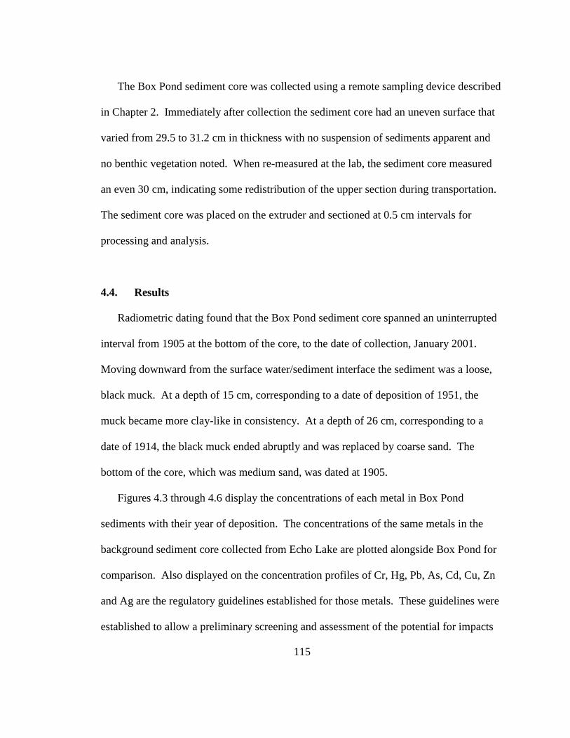
115

The Box Pond sediment core was collected using a remote sampling device described

in Chapter 2. Immediately after collection the sediment core had an uneven surface that

varied from 29.5 to 31.2 cm in thickness with no suspension of sediments apparent and

no benthic vegetation noted. When re-measured at the lab, the sediment core measured

an even 30 cm, indicating some redistribution of the upper section during transportation.

The sediment core was placed on the extruder and sectioned at 0.5 cm intervals for

processing and analysis.

4.4. Results

Radiometric dating found that the Box Pond sediment core spanned an uninterrupted

interval from 1905 at the bottom of the core, to the date of collection, January 2001.

Moving downward from the surface water/sediment interface the sediment was a loose,

black muck. At a depth of 15 cm, corresponding to a date of deposition of 1951, the

muck became more clay-like in consistency. At a depth of 26 cm, corresponding to a

date of 1914, the black muck ended abruptly and was replaced by coarse sand. The

bottom of the core, which was medium sand, was dated at 1905.

Figures 4.3 through 4.6 display the concentrations of each metal in Box Pond

sediments with their year of deposition. The concentrations of the same metals in the

background sediment core collected from Echo Lake are plotted alongside Box Pond for

comparison. Also displayed on the concentration profiles of Cr, Hg, Pb, As, Cd, Cu, Zn

and Ag are the regulatory guidelines established for those metals. These guidelines were

established to allow a preliminary screening and assessment of the potential for impacts

116

to aquatic life (National Oceanic and Atmospheric Administration 1999). As explained

in Chapter 1, the Effects Range Low (ERL) and Effects Range Median (ERM) values

were established as guidelines to evaluate the potential for sediment toxicity to aquatic

organisms. Quality control and quality assurance measures are described in Chapter 2

and the methods used for determining the geochronology are described in Appendix III.

Figure 4.3 shows the sediment concentration profiles for Al, Sr, Sc and Co. These

metals are typically used for determining the crustal contribution of metals due to erosion

from native soils and rock. Figure 4.4 shows the sediment concentration profiles for Fe,

Mn, Cr and TOC. These metals and TOC provide insight into the chemistry of the

depositional environment. Figure 4.5 shows the sediment concentration profiles for Hg,

Pb, As and Cd. These metals have wide-spread anthropogenic uses and are most

commonly associated with toxic effects. Figure 4.6 shows the sediment concentration

profiles for Cu, Zn, Sn and Ag. These metals are typically associated with anthropogenic

discharges. At high concentrations these metals may also adversely affect aquatic life.

117

Figure 4.3. Sediment concentration profiles of Al, Sr, Sc and Co.

1900

1910

1920

1930

1940

1950

1960

1970

1980

1990

2000

0 20 40 60 80

Ye

ar

a. Aluminum (mg/g)

Box Pond

Echo Lake

1900

1910

1920

1930

1940

1950

1960

1970

1980

1990

2000

0 50 100 150 200

Ye

ar

b. Strontium (ug/g)

Box Pond

Echo Lake

1900

1910

1920

1930

1940

1950

1960

1970

1980

1990

2000

0 20 40 60

Ye

ar

c. Scandium (ug/g)

Box Pond

Echo Lake

1900

1910

1920

1930

1940

1950

1960

1970

1980

1990

2000

0 5 10 15 20

Ye

ar

d. Cobalt (ug/g)

Box Pond

Echo Lake

118

Figure 4.4. Sediment concentration profiles of Fe, Mn, Cr, and TOC.

1900

1910

1920

1930

1940

1950

1960

1970

1980

1990

2000

0 50 100

Ye

ar

a. Iron (mg/g)

Box Pond

Echo Lake

1900

1910

1920

1930

1940

1950

1960

1970

1980

1990

2000

0 500 1000

Ye

ar

b. Manganese (ug/g)

Box Pond

Echo Lake

1900

1910

1920

1930

1940

1950

1960

1970

1980

1990

2000

0 100 200 300

Ye

ar

c. Chromium (ug/g)

Box Pond Echo Lake ERL ERM

1900

1910

1920

1930

1940

1950

1960

1970

1980

1990

2000

0 5 10 15 20

Ye

ar

d. TOC (moles/kg)

Box Pond

Echo Lake

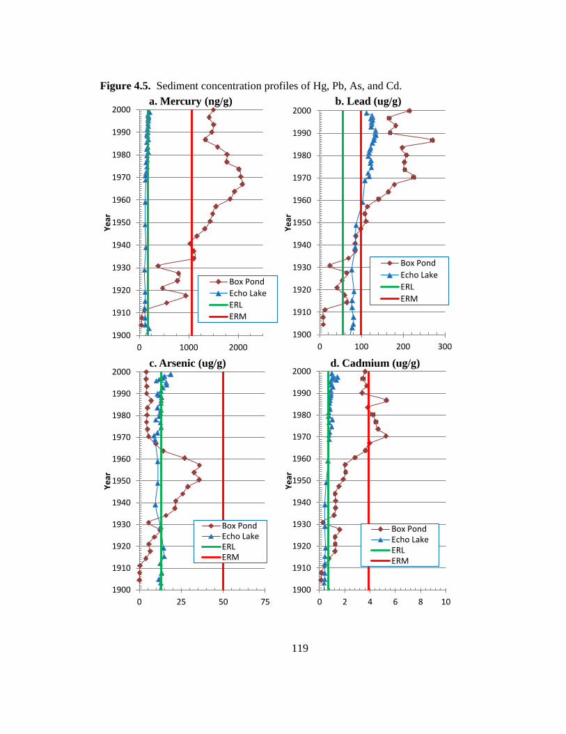
119

Figure 4.5. Sediment concentration profiles of Hg, Pb, As, and Cd.

1900

1910

1920

1930

1940

1950

1960

1970

1980

1990

2000

0 1000 2000

Ye

ar

a. Mercury (ng/g)

Box Pond

Echo Lake

ERL

ERM

1900

1910

1920

1930

1940

1950

1960

1970

1980

1990

2000

0 100 200 300

Ye

ar

b. Lead (ug/g)

Box Pond

Echo Lake

ERL

ERM

1900

1910

1920

1930

1940

1950

1960

1970

1980

1990

2000

0 25 50 75

Ye

ar

c. Arsenic (ug/g)


1900

1910

1920

1930

1940

1950

1960

1970

1980

1990

2000

0 2 4 6 8 10

Ye

ar

d. Cadmium (ug/g)


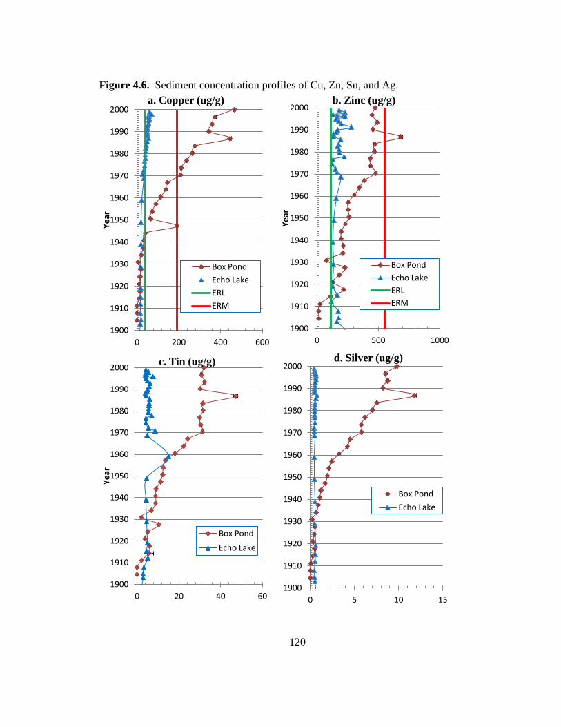
120

Figure 4.6. Sediment concentration profiles of Cu, Zn, Sn, and Ag.

1900

1910

1920

1930

1940

1950

1960

1970

1980

1990

2000

0 200 400 600

Ye

ar

a. Copper (ug/g)

Box Pond

Echo Lake

ERL

ERM

1900

1910

1920

1930

1940

1950

1960

1970

1980

1990

2000

0 500 1000

Ye

ar

b. Zinc (ug/g)

Box Pond

Echo Lake

ERL

ERM

1900

1910

1920

1930

1940

1950

1960

1970

1980

1990

2000

0 20 40 60

Ye

ar

c. Tin (ug/g)

Box Pond

Echo Lake

1900

1910

1920

1930

1940

1950

1960

1970

1980

1990

2000

0 5 10 15

d. Silver (ug/g)

Box Pond

Echo Lake

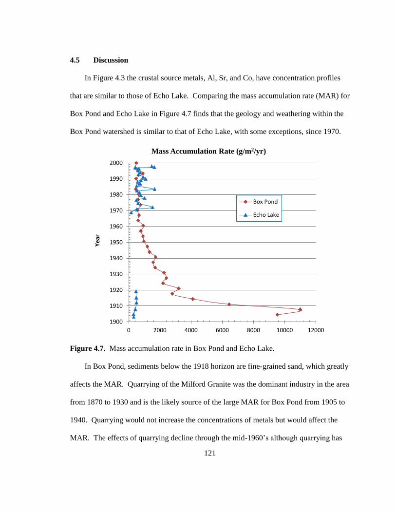
121

4.5 Discussion

In Figure 4.3 the crustal source metals, Al, Sr, and Co, have concentration profiles

that are similar to those of Echo Lake. Comparing the mass accumulation rate (MAR) for

Box Pond and Echo Lake in Figure 4.7 finds that the geology and weathering within the

Box Pond watershed is similar to that of Echo Lake, with some exceptions, since 1970.

Figure 4.7. Mass accumulation rate in Box Pond and Echo Lake.

In Box Pond, sediments below the 1918 horizon are fine-grained sand, which greatly

affects the MAR. Quarrying of the Milford Granite was the dominant industry in the area

from 1870 to 1930 and is the likely source of the large MAR for Box Pond from 1905 to

1940. Quarrying would not increase the concentrations of metals but would affect the

MAR. The effects of quarrying decline through the mid-1960’s although quarrying has

1900

1910

1920

1930

1940

1950

1960

1970

1980

1990

2000

0 2000 4000 6000 8000 10000 12000

Ye

ar

Mass Accumulation Rate (g/m2/yr)

Box Pond

Echo Lake

122

remained active through the present. The Echo Lake MAR profile is missing the period

from 1920 to 1967 because that period is an unconformity for the Echo Lake sediments.

The concentration profiles of many metals in Box Pond sediments differ greatly over

the metal concentrations in sediments that were deposited contemporaneously in Echo

Lake. These differences are the result of the contrast in the anthropogenic uses in each

watershed during those periods.

4.5.1 Anthropogenic Addition of Metals to Sediments

The concentration of metals in Box Pond sediments that differ significantly from the

sediment concentrations in the background location include: Cr, Hg, Pb, As, Cd, Cu, Sn,

Zn, and Ag. Although the concentration profiles of each of these metals display subtle

differences, they may be divided into two groups. The first group, Cr, Hg, Pb, Cd, Sn,

and Zn share a common profile in that their concentrations increase beginning in the mid-

1940’s, peak in 1970 and then either remain constant or decrease in younger sediments.

The concentrations for these metals are also much greater than those of the background

location. This behavior may be due to the metal contribution of a single source. The

second group: As, Cu and Ag display distinct concentration profiles that indicate

potentially different sources of these metals.

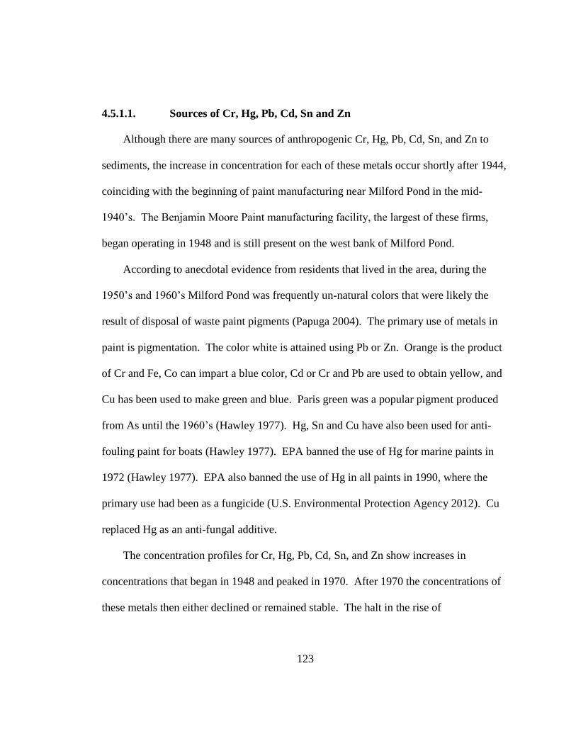
123

4.5.1.1. Sources of Cr, Hg, Pb, Cd, Sn and Zn

Although there are many sources of anthropogenic Cr, Hg, Pb, Cd, Sn, and Zn to

sediments, the increase in concentration for each of these metals occur shortly after 1944,

coinciding with the beginning of paint manufacturing near Milford Pond in the mid-

1940’s. The Benjamin Moore Paint manufacturing facility, the largest of these firms,

began operating in 1948 and is still present on the west bank of Milford Pond.

According to anecdotal evidence from residents that lived in the area, during the

1950’s and 1960’s Milford Pond was frequently un-natural colors that were likely the

result of disposal of waste paint pigments (Papuga 2004). The primary use of metals in

paint is pigmentation. The color white is attained using Pb or Zn. Orange is the product

of Cr and Fe, Co can impart a blue color, Cd or Cr and Pb are used to obtain yellow, and

Cu has been used to make green and blue. Paris green was a popular pigment produced

from As until the 1960’s (Hawley 1977). Hg, Sn and Cu have also been used for anti-

fouling paint for boats (Hawley 1977). EPA banned the use of Hg for marine paints in

1972 (Hawley 1977). EPA also banned the use of Hg in all paints in 1990, where the

primary use had been as a fungicide (U.S. Environmental Protection Agency 2012). Cu

replaced Hg as an anti-fungal additive.

The concentration profiles for Cr, Hg, Pb, Cd, Sn, and Zn show increases in

concentrations that began in 1948 and peaked in 1970. After 1970 the concentrations of

these metals then either declined or remained stable. The halt in the rise of

124

concentrations in post-1970’s sediment may be due to changes in business practices,

economic conditions, or perhaps public pressure.

In eastern Massachusetts, the general economy struggled through the 1970’s which

may have either caused a reduced demand for paint during the 1970’s or perhaps caused

the manufacturing operations for some of the paint lines to move to other locations

(Schwenk 2001). Changes in manufacturing technique or material handling may have

occurred in 1970 that stopped or re-directed discharges to the Charles River.

The decline in metal concentrations after 1970 may have also been due to a rising

environmental awareness among the public. Following the first Earth Day in April 1970

and the creation of EPA by Congress in July 1970, public awareness would have

increased. Complaints from the public regarding the changing colors of the pond, or the

increased awareness by the paint manufacturers may have increased their diligence in

handling wastes.

Environmental regulation was not the cause of the 1970 decline as EPA was only

formed in December, 1970. Although many environmental regulations were enacted in

the early 1970’s, such as the Clean Water Act (1972), implementation of those laws

occurred several years later. For instance, the increase of Pb in Box Pond sediments

stopped in 1970, yet the ban on the use of Pb in paint was implemented in 1977 (U.S.

Consumer Product Safety Commission 1977). EPA announced the phase out of Pb in

gasoline in December 1973 and that ban was not complete until 1996.

The dating of the sediment core is crucial in assessing these dates and sources. The

confidence in the assigned dates is strong. The Box Pond sediment core was found to

125

present a strong 137

Cs peak at 1964 and the assigned uncertainty using the excess 210

Pb

gamma detection techniques was less than 1 year for the entire sediment core as shown in

Table III.1.

As shown in Figure 4.5b, the concentration of Pb in Box Pond approximates Echo

Lake’s concentration until 1957, after which the concentration in Box Pond nearly

doubles. The delay between the start of paint production in the late 1940’s and the

increase in Pb after 1957 could be due to the nature of the waste Pb, which could be

bound with other paint components and perhaps have a greater residence time in Milford

Pond.

After the 1970 peak, the concentration of Pb remains steady for more than 10 years

potentially due to the travel time of the Pb-particulates from Milford Pond to Box Pond.

The 1987 peak may be due to an upstream erosion event that will be discussed later as it

has implications for all metals. After 1987, Pb concentrations begin to decline parallel to

those in Echo Lake. This may be due in part to the Clean Air Act eliminating the

discharge of Pb from automobile emissions.

The Box Pond Hg sediment concentration profile in Figure 4.5a displays key

differences from the background Hg sediment of Echo Lake. The Box Pond sediments

show a relatively constant concentration of Hg in sediments from 1914 to 1940 that are

approximately six times the concentration of Echo Lake sediments being deposited in the

same period. Possible sources of this increase are the manufacturers that made electrical

switches in the Milford area or dental amalgams. The population of Milford from 1910

to 1940 was 12,000 to 15,000 and poor practices in the disposal of dental amalgams may

126

also account for this increase in concentration (Wallace et al. 2004). The population of

the Echo Lake watershed during the same time was approximately 20 to 40 persons and

there were no businesses or industry active in the Echo Lake watershed.

After 1944, the concentration of Hg in sediment increased dramatically, coincident

with the start of paint manufacturing in the area. The same increase in concentration after

1957 that occurred for Pb also occurs for Hg. The appearance of Hg in the Box Pond

sediments in 1944 indicates that the Hg was mobile in the water column and easily

distributed. By 1970 the concentration of Hg in sediment was nearly 20 times the value

in Echo Lake. Similar to Pb, there is no definitive reason for the decline in concentration

of Hg in Box Pond sediments after 1970 other than those cited above. The concentration

of Hg continued to decline until 1987. After 1987 the concentration profile for Hg

remains approximately 7 times that of Echo Lake but appears to parallel the increase in

concentration found in Echo Lake. This indicates a continuing source of Hg that is

increasing at the same rate throughout the watershed. This may be the result of

atmospheric fallout.

Cr, Cd, Sn and Zn display sediment concentration profiles that are remarkably

similar and bear many of the same features of Hg and Pb, a steady rise in concentration

after 1944, a larger rate of concentration increase after 1957, a peak at 1970, and then

either steady or declining concentrations. Zn and Sn appear to slightly increase after

1970 which may be due to additional anthropogenic discharges from automobile tires and

building materials (Davis et al. 2001). Sn has uses in plating of steel and manufacture of

bronze. These uses are prevalent in food canning and in plumbing fixtures (Hawley

127

1977). It is unknown if antifouling paints using organotin were produced and discharged

in the Milford area. Paint manufacture continued through at least the early 1980’s and

Benjamin Moore, a major manufacturer of paint, maintained a facility on the west bank

of the Charles River as late as 2011 (Goyette 1982).

4.5.1.2. Sources of As, Cu and Ag

Although As, Cu and Ag may be used as pigments in paint as described in the

preceding section, the concentration profiles of these metals differ greatly over those of

the other metals. Paint manufacture may still be one source, but the difference in the

concentration profiles suggest that processes in the water column or sediment act on

those metals differently.

The sediment concentration profiles of Cu and Ag in Figures 4.6a and 4.6d,

respectively, appear identical. A comparison to the background concentrations and an

examination of the scales reveal subtle differences that may be diagnostic of sources. Cu

has a concentration similar to its background until 1947. The increase in sediment

concentration in Box Pond is continuous and at the time of core collection was greater

than 4 times the concentration of Echo Lake sediment Cu. Because Cu is an important

pigment in paint and is also used as a fungicide and anti-fouling paint for boats, its

simultaneous increase with the start of the paint industry indicates that paint may be the

primary source at that time. The continued increase in sediment concentration after 1970

may be due to a new source such as automobile brakes or corrosion from residential

128

plumbing (Davis et al. 2001). During ICP-MS analysis the isotopes of 65

Cu and 63

Cu

were measured and are shown in Figure 4.8.

Figure 4.8. Ratio of

65Cu relative to

63Cu in Box Pond.

The change in isotope ratio suggests that the source of Cu after 1980 differs from

that before 1980. For instance, prior to 1908 and the beginning of public sewage

collection and treatment, the ratio of concentrations of 65

Cu and 63

Cu indicated that 63

Cu

was more prevalent. Figure 4.8 shows a break in the general trend after 1980, suggesting

that another source of Cu, more enriched in 63

Cu was deposited in Box Pond sediment at

that time. That source may be automobile brakes or Cu dissolved from plumbing in

homes.

The sediment concentration for Ag in Box Pond departs from the background

concentration in the mid-1930’s and increases continuously thereafter. The beginning of

the increase in Ag concentration is before paint manufacturing began, but approximately

1900

1910

1920

1930

1940

1950

1960

1970

1980

1990

2000

1 1.1 1.2

Ye

ar

65Cu / 63Cu

in Box Pond

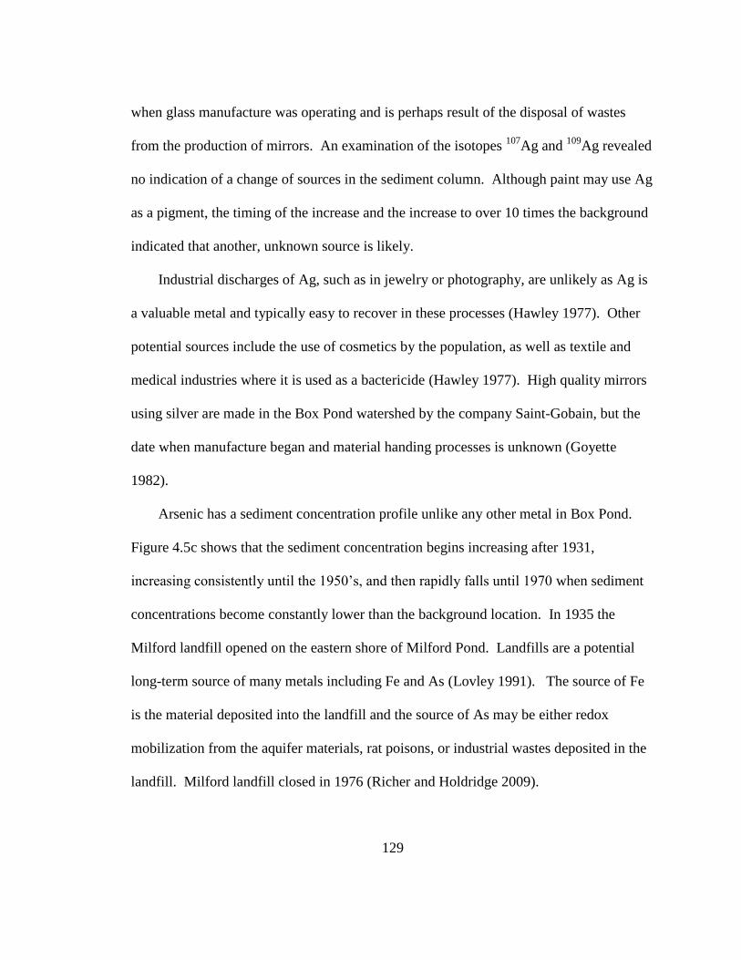
129

when glass manufacture was operating and is perhaps result of the disposal of wastes

from the production of mirrors. An examination of the isotopes 107

Ag and 109

Ag revealed

no indication of a change of sources in the sediment column. Although paint may use Ag

as a pigment, the timing of the increase and the increase to over 10 times the background

indicated that another, unknown source is likely.

Industrial discharges of Ag, such as in jewelry or photography, are unlikely as Ag is

a valuable metal and typically easy to recover in these processes (Hawley 1977). Other

potential sources include the use of cosmetics by the population, as well as textile and

medical industries where it is used as a bactericide (Hawley 1977). High quality mirrors

using silver are made in the Box Pond watershed by the company Saint-Gobain, but the

date when manufacture began and material handing processes is unknown (Goyette

1982).

Arsenic has a sediment concentration profile unlike any other metal in Box Pond.

Figure 4.5c shows that the sediment concentration begins increasing after 1931,

increasing consistently until the 1950’s, and then rapidly falls until 1970 when sediment

concentrations become constantly lower than the background location. In 1935 the

Milford landfill opened on the eastern shore of Milford Pond. Landfills are a potential

long-term source of many metals including Fe and As (Lovley 1991). The source of Fe

is the material deposited into the landfill and the source of As may be either redox

mobilization from the aquifer materials, rat poisons, or industrial wastes deposited in the

landfill. Milford landfill closed in 1976 (Richer and Holdridge 2009).

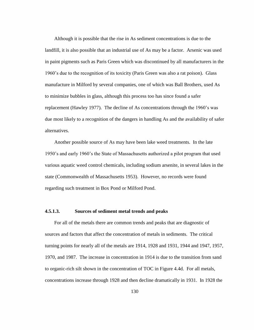
130

Although it is possible that the rise in As sediment concentrations is due to the

landfill, it is also possible that an industrial use of As may be a factor. Arsenic was used

in paint pigments such as Paris Green which was discontinued by all manufacturers in the

1960’s due to the recognition of its toxicity (Paris Green was also a rat poison). Glass

manufacture in Milford by several companies, one of which was Ball Brothers, used As

to minimize bubbles in glass, although this process too has since found a safer

replacement (Hawley 1977). The decline of As concentrations through the 1960’s was

due most likely to a recognition of the dangers in handling As and the availability of safer

alternatives.

Another possible source of As may have been lake weed treatments. In the late

1950’s and early 1960’s the State of Massachusetts authorized a pilot program that used

various aquatic weed control chemicals, including sodium arsenite, in several lakes in the

state (Commonwealth of Massachusetts 1953). However, no records were found

regarding such treatment in Box Pond or Milford Pond.

4.5.1.3. Sources of sediment metal trends and peaks

For all of the metals there are common trends and peaks that are diagnostic of

sources and factors that affect the concentration of metals in sediments. The critical

turning points for nearly all of the metals are 1914, 1928 and 1931, 1944 and 1947, 1957,

1970, and 1987. The increase in concentration in 1914 is due to the transition from sand

to organic-rich silt shown in the concentration of TOC in Figure 4.4d. For all metals,

concentrations increase through 1928 and then decline dramatically in 1931. In 1928 the

131

POTW increased capacity, although details of the work were unavailable, such work on

the POTW may have created the potential for flushing of settling ponds. The subsequent

1931 decline in sediment concentration that is present in the concentration profiles for all

metals and TOC could be the new treatment lagoons absorbing much of the new flow.

The concentration profiles of all metals resume their general trends after the 1931

decline and remain relatively constant in concentration until 1944 or 1947 after which a

general increase in concentration occurs. It is possible that some of the increase in

sediment metal concentrations after 1941 could be due to increased production of many

metal items in World War II. But the largest increase after 1944 for many of the metals

is likely due to production at the paint companies.

In 1957 the POTW increased capacity again, but unlike 1928, rate of increase in

concentrations for all metals appear to increase after this date, perhaps due to the general

economic expansion in the late 1950’s and early 1960’s (Schwenk 2001). Concentrations

increase until 1970 and then either decline or remain relatively constant except for Cu

and Ag.

After 1970 the most prominent feature is a peak at 1987. Twelve of the fifteen

metals have a concentration peak in 1987 and for nine of the fifteen metals it is their

maximum concentration in the sediment record. In 1986 the POTW was upgraded to

include tertiary treatment. Tertiary treatment typically produces a discharge that is

almost potable. The subsequent increase in sediment metal concentration in 1987 could

be due to either flushing of the old sedimentation ponds, or the discharge from the POTW

being re-routed to a new location, disturbing sediments containing high concentrations of

132

metals, when the old ponds were emptied. The estimated flow from the POTW may have

been higher than typical flows and in the existing narrow channel would be capable of

disturbing existing, historic sediments and depositing them in Box Pond in 1987

(Simpson et al. 1998).

Approximately 1 km upstream of Box Pond, and downstream of the POTW, a

woolen mill operated during the 1800’s, burned down in 1868, and was not re-built

(Partridge 1919). Woolen mills discharge many waste dyes and metal-containing

“liquors.” Table 4.2 compares the concentrations of Box Pond sediments for 1987 to

sediments at a Superfund site woolen mill in Corrina, Maine (U.S. Environmental

Protection Agency 2004).

Table 4.2. Comparison of maximum sediment metal concentrations, Eastland Woolen

Mills Superfund Site in Corrina, Maine and Box Pond sediments deposited in 1987.

Superfund Site Box Pond Sediment

µg/g µg/g

As 16 7.1

Cd 56 5.3

Cr 390 174

Cu 49 445

Pb 330 270

Hg 1.2 1.3

Ag 0.56 11.8

Zn 2600 683

Table 4.2 shows that the metals in the Superfund Site sediments and Box Pond

sediments have very similar concentrations of metals, most notably Hg and Pb. The

changes in operations at the POTW in 1928, 1957, and 1987 coinciding with changes in

the concentration, or rate of concentration increase, for many of the metals in Box Pond

133

sediments, indicates that the POTW exerts a significant influence on metal

concentrations.

The POTW does not accept raw industrial discharges and discharges treated water at

an average approximate rate of 1 m3 min

-1. The discharge limits are based on an

allowable flow of 18x106 l day

-1 (monthly average) and include the discharge of total

suspended solids (TSS) of 100 to 800 kg day-1

, as well as dissolved components

including Al (1500 g day-1

), Cu (300 to 500 g day-1

), and Pb (68 g day-1

) (Commonwealth

of Massachusetts 2010). There is no requirement to determine the concentration of the

TSS component of the flow. The uncharacterized TSS may be the source of the excess

concentrations of Hg, Pb, Cd, Cr, Cu, Zn, Sn and Ag that continue to the top of the

sediment core. The concentrations of all these metals in sediments that were deposited

after 1970 and up to 2000 greatly exceed those of the background location, Echo Lake.

Although the POTW is a tertiary treatment plant, releases of untreated water can

occur. On August 9, 1999, following a one-inch rainstorm the previous night, Box Pond,

4 km downstream of the POTW, had a distinct sewage smell. Because the POTW

accepts residential sewage, and there is an industrial pretreatment program that addresses

industrial discharges, the concentration of metals discharged may also be a function of

population (U.S. Environmental Protection Agency 1999).

The % Commercial, Industrial and Transportation (%CIT) is used by several authors

to gauge the effects of land use as it is a measure of altered and impervious area

(Chalmers et al. 2007; Coles et al. 2010). In Chapter 3 an estimate of the %CIT for the

Echo Lake watershed was calculated because the watershed is small and the land use

134

changes relatively recent and can be estimated using maps and building permits. The

Milford area does not share that character and no historic values of %CIT are available,

nor are there any reasonable means of estimating such a value. Moreover, the %CIT

value may not be appropriate in the instance of historic industrial discharges. To

examine sediment metal concentrations as industrial discharges are controlled after 1970

requires a common metric of measure. Population remains the singular available statistic

that may provide insight to sediment metal concentrations. The growth in population of

Milford is shown below on Figure 4.9.

Figure 4.9. Historical population of Milford, Massachusetts, 1905 to 2001.

Population density and the amount of disturbed watershed is an indicator of water

quality and hence sediment concentrations due to the storm water runoff from impervious

areas (Chalmers et al. 2007; Coles et al. 2010). The population of Milford was higher

than the Echo Lake watershed, which had only 16 homes until 1969. The population

0

5,000

10,000

15,000

20,000

25,000

30,000

1880 1890 1900 1910 1920 1930 1940 1950 1960 1970 1980 1990 2000

Po

pu

lati

on

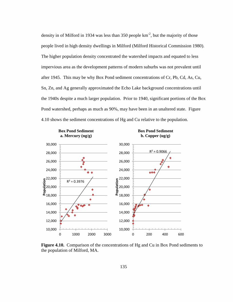
135

density in of Milford in 1934 was less than 350 people km-2

, but the majority of those

people lived in high density dwellings in Milford (Milford Historical Commission 1980).

The higher population density concentrated the watershed impacts and equated to less

impervious area as the development patterns of modern suburbs was not prevalent until

after 1945. This may be why Box Pond sediment concentrations of Cr, Pb, Cd, As, Cu,

Sn, Zn, and Ag generally approximated the Echo Lake background concentrations until

the 1940s despite a much larger population. Prior to 1940, significant portions of the Box

Pond watershed, perhaps as much as 90%, may have been in an unaltered state. Figure

4.10 shows the sediment concentrations of Hg and Cu relative to the population.

Figure 4.10. Comparison of the concentrations of Hg and Cu in Box Pond sediments to

the population of Milford, MA.

R² = 0.3976

10,000

12,000

14,000

16,000

18,000

20,000

22,000

24,000

26,000

28,000

30,000

0 1000 2000 3000

Po

pu

lati

on

Box Pond Sediment

a. Mercury (ng/g)

R² = 0.9066

10,000

12,000

14,000

16,000

18,000

20,000

22,000

24,000

26,000

28,000

30,000

0 200 400 600

Po

pu

lati

on

Box Pond Sediment

b. Copper (ug/g)

136

Figure 4.10 contrasts the concentration of Hg and Cu with the population over the

length of the sediment core. The industrial discharge dominates the Hg profile between

the populations of 15,000 and 23,000 in Figure 4.10 a., which corresponds to 1940 and

1980, respectively. But an examination of trends before 1940 and after 1987, before and

after industrial influences, indicates that the concentration may be affected by population.

The Hg concentration profile in Figure 4.10 a. shows linearity that may be a function of

population from 1905 until the population was approximately 15,000, corresponding to

the early 1940’s. This would correspond to the period before paint manufacture began.

During this time period many products containing Hg were available to the public

(Hawley 1977). Milford was a large city through this period and it is likely that dental

offices were common. Dental fillings may have contributed Hg to the waste stream of

the POTW (Wallace et al. 2004). The relationship between Hg and population from 1905

to 1944 has an R2 value of 0.76 and the slope of the regression, or rate of increase in

concentration during this period, is approximately 29 ng yr-1

.

The Hg profile assumes a linear increase after the population is 24,708 in1987 to the

top of the sediment core in 2000 that approximates that of the 1905 to 1944 interval. A

regression of this period found an increase in concentration of 11 ng yr-1

and an R2 of 0.6.

Caution should be used regarding this regression statistic as the number of observations is

small (n=4) and these sediments are close to the surface water increasing the potential for

bioturbation and other processes that may affect the concentration of Hg. The average

concentration of Hg in the period after 1987 (>1400 ng g-1

) is well above that of Echo

Lake, which had an average concentration of 175 ng g-1

for the same period. By

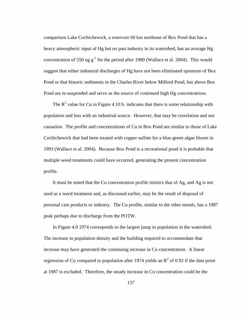
137

comparison Lake Cochichewick, a reservoir 60 km northeast of Box Pond that has a

heavy atmospheric input of Hg but no past industry in its watershed, has an average Hg

concentration of 550 ng g-1

for the period after 1980 (Wallace et al. 2004). This would

suggest that either industrial discharges of Hg have not been eliminated upstream of Box

Pond or that historic sediments in the Charles River below Milford Pond, but above Box

Pond are re-suspended and serve as the source of continued high Hg concentrations.

The R2 value for Cu in Figure 4.10 b. indicates that there is some relationship with

population and less with an industrial source. However, that may be correlation and not

causation. The profile and concentrations of Cu in Box Pond are similar to those of Lake

Cochichewick that had been treated with copper sulfate for a blue-green algae bloom in

1993 (Wallace et al. 2004). Because Box Pond is a recreational pond it is probable that

multiple weed treatments could have occurred, generating the present concentration

profile.

It must be noted that the Cu concentration profile mimics that of Ag, and Ag is not

used as a weed treatment and, as discussed earlier, may be the result of disposal of

personal care products or industry. The Cu profile, similar to the other metals, has a 1987

peak perhaps due to discharge from the POTW.

In Figure 4.9 1974 corresponds to the largest jump in population in the watershed.

The increase in population density and the building required to accommodate that

increase may have generated the continuing increase in Cu concentration. A linear

regression of Cu compared to population after 1974 yields an R2 of 0.92 if the data point

at 1987 is excluded. Therefore, the steady increase in Cu concentration could be the

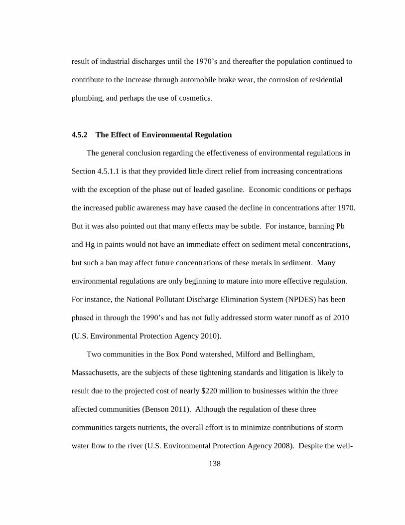
138

result of industrial discharges until the 1970’s and thereafter the population continued to

contribute to the increase through automobile brake wear, the corrosion of residential

plumbing, and perhaps the use of cosmetics.

4.5.2 The Effect of Environmental Regulation

The general conclusion regarding the effectiveness of environmental regulations in

Section 4.5.1.1 is that they provided little direct relief from increasing concentrations

with the exception of the phase out of leaded gasoline. Economic conditions or perhaps

the increased public awareness may have caused the decline in concentrations after 1970.

But it was also pointed out that many effects may be subtle. For instance, banning Pb

and Hg in paints would not have an immediate effect on sediment metal concentrations,

but such a ban may affect future concentrations of these metals in sediment. Many

environmental regulations are only beginning to mature into more effective regulation.

For instance, the National Pollutant Discharge Elimination System (NPDES) has been

phased in through the 1990’s and has not fully addressed storm water runoff as of 2010


Two communities in the Box Pond watershed, Milford and Bellingham,

Massachusetts, are the subjects of these tightening standards and litigation is likely to

result due to the projected cost of nearly $220 million to businesses within the three

affected communities (Benson 2011). Although the regulation of these three

communities targets nutrients, the overall effort is to minimize contributions of storm

water flow to the river (U.S. Environmental Protection Agency 2008). Despite the well-

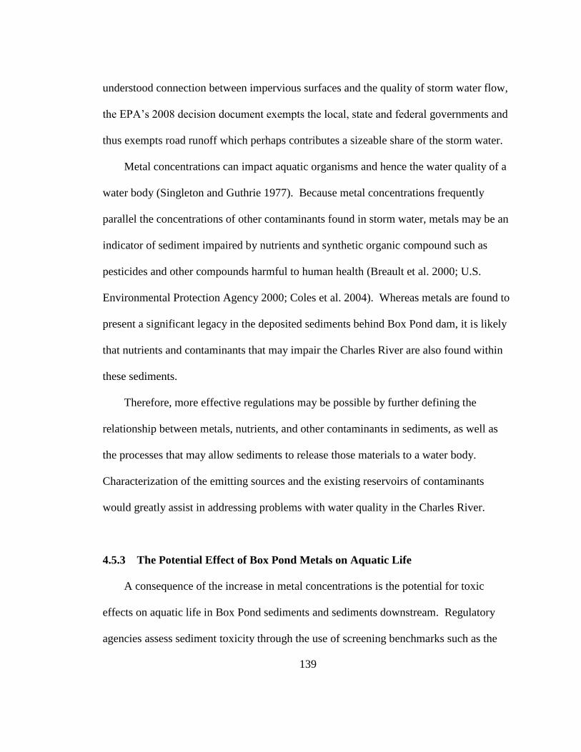
139

understood connection between impervious surfaces and the quality of storm water flow,

the EPA’s 2008 decision document exempts the local, state and federal governments and

thus exempts road runoff which perhaps contributes a sizeable share of the storm water.

Metal concentrations can impact aquatic organisms and hence the water quality of a

water body (Singleton and Guthrie 1977). Because metal concentrations frequently

parallel the concentrations of other contaminants found in storm water, metals may be an

indicator of sediment impaired by nutrients and synthetic organic compound such as

pesticides and other compounds harmful to human health (Breault et al. 2000; U.S.

Environmental Protection Agency 2000; Coles et al. 2004). Whereas metals are found to

present a significant legacy in the deposited sediments behind Box Pond dam, it is likely

that nutrients and contaminants that may impair the Charles River are also found within

these sediments.

Therefore, more effective regulations may be possible by further defining the

relationship between metals, nutrients, and other contaminants in sediments, as well as

the processes that may allow sediments to release those materials to a water body.

Characterization of the emitting sources and the existing reservoirs of contaminants

would greatly assist in addressing problems with water quality in the Charles River.

4.5.3 The Potential Effect of Box Pond Metals on Aquatic Life

A consequence of the increase in metal concentrations is the potential for toxic

effects on aquatic life in Box Pond sediments and sediments downstream. Regulatory

agencies assess sediment toxicity through the use of screening benchmarks such as the

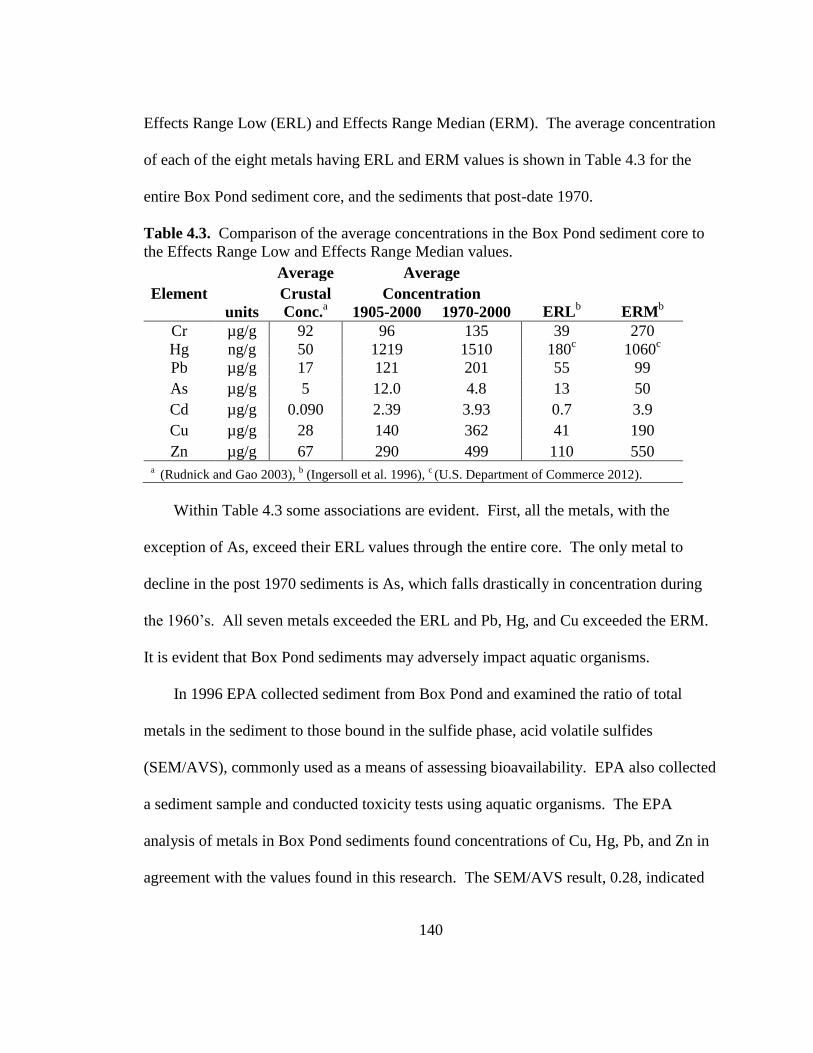
140

Effects Range Low (ERL) and Effects Range Median (ERM). The average concentration

of each of the eight metals having ERL and ERM values is shown in Table 4.3 for the

entire Box Pond sediment core, and the sediments that post-date 1970.

Table 4.3. Comparison of the average concentrations in the Box Pond sediment core to

the Effects Range Low and Effects Range Median values.

Average Average

Element Crustal Concentration

units Conc.a 1905-2000 1970-2000 ERL

b ERM

b

Cr µg/g 92 96 135 39 270

Hg ng/g 50 1219 1510 180c 1060

c

Pb µg/g 17 121 201 55 99

As µg/g 5 12.0 4.8 13 50

Cd µg/g 0.090 2.39 3.93 0.7 3.9

Cu µg/g 28 140 362 41 190

Zn µg/g 67 290 499 110 550 a (Rudnick and Gao 2003),

b (Ingersoll et al. 1996),

c (U.S. Department of Commerce 2012).

Within Table 4.3 some associations are evident. First, all the metals, with the

exception of As, exceed their ERL values through the entire core. The only metal to

decline in the post 1970 sediments is As, which falls drastically in concentration during

the 1960’s. All seven metals exceeded the ERL and Pb, Hg, and Cu exceeded the ERM.

It is evident that Box Pond sediments may adversely impact aquatic organisms.

In 1996 EPA collected sediment from Box Pond and examined the ratio of total

metals in the sediment to those bound in the sulfide phase, acid volatile sulfides

(SEM/AVS), commonly used as a means of assessing bioavailability. EPA also collected

a sediment sample and conducted toxicity tests using aquatic organisms. The EPA

analysis of metals in Box Pond sediments found concentrations of Cu, Hg, Pb, and Zn in

agreement with the values found in this research. The SEM/AVS result, 0.28, indicated

141

that much of the metals were bound in the sulfide phase and therefore not bio-available.

The EPA toxicity test of the Box Pond sediment corroborated this finding with the result

that 89% of the test organisms Chironomus tentans and 96% of Hyallela azteca

organisms survived the 10-day test indicating no toxicity in these sediments (U.S.


Although metals in Box Pond sediment may not adversely impact aquatic organisms

in its present state, re-suspension of these sediments may have toxic effects further

downstream. Although the metals in Box Pond are maintained in the sulfide phase,

redistribution downstream may alter the particulate-metal complex and create a more bio-

available complex that affects organisms in other stream environments (Rogers et al.

2002).

4.6 Conclusions

The concentrations of Cr, Hg, Pb, As, Cd, Cu, Zn, Sn and Ag in Box Pond sediments

were greatly elevated above the background concentrations in Echo Lake. Several

industries have operated and discharged metals in the Box Pond watershed, but it is likely

that paint manufacturing is responsible for the majority of those metals. Although the

concentrations of metals in more recent sediments are lower than in the period from the

mid-1940’s to 1970, the metals with established guidelines to assess potential toxicity to

aquatic organisms exceeded toxicity threshold values. This indicates that the potential

for sediments to adversely affect aquatic life in Box Pond and further downstream.

142

In Box Pond the long-term high concentrations of Hg, Pb and other metals may

likely be the result of the contribution of sediments and soils that are eroded from

upstream sources and were deposited in Box Pond. The association of metal

concentrations and land use is obscured by this contribution and use of the land use

metric of %CIT was ineffective because of the historic industrial discharges.

Population may still be a factor in metal concentration trends in sediments deposited

after 1970. The concentration profile of Hg increases with population after 1987 that

may be the result of dental amalgams and other sources within the population. The

discharge resulting from work at the POTW may have impacted nearly all metal

concentrations in Box Pond in 1928, 1957, and 1987. In 1987 the expansion of the

treatment plant may have re-suspended historic, heavily contaminated sediments and

distributed the metals further downstream and to Box Pond.

Although environmental regulations may have not had a direct, significant impact on

metals in sediment, the relationships between the sources and reservoirs of allochthonous,

anthropogenic metals may be significant with respect to future environmental regulation.

The high concentrations and increases in metal concentrations in Box Pond sediments is

the result of sources that include atmospheric fallout transmitted by storm water, direct

industrial discharges, discharge from a sewage treatment works, and the erosion or re-

suspension of soils and sediment that contain metals discharged in the past. The

development of methods to determine the flux of anthropogenic metals into a watershed

and the factors that affect the residence time of those metals in the watershed would

143

greatly enhance environmental regulation not only of metal concentrations but other

contaminants as well.

144

CHAPTER 5

COPPER, ZINC, LEAD AND MERCURY IN THE CHARLES RIVER

Abstract

The concentrations of Cu, Zn, Pb and Hg in the upper 3 cm of sediments at 13

locations along the Charles River were examined to determine the concentrations and

likely sources of these metals that were deposited over an approximate 10-year period.

The concentrations of these metals were found to exceed regulatory guidelines for

toxicity throughout much of the river and were higher than other similar urban water

bodies. The population density and the percentage of Commercial, Industrial and

Transportation network (%CIT) for each community bordering the river was compared to

the concentrations of these metals. It was determined that the %CIT, a function of storm

water runoff, was related to the sediment metal concentrations. Simple regression models

were developed for Cu and Hg that demonstrated the relationship of total organic carbon

to their concentrations in sediments. The models indicated that improvements in storm

water management may decrease the concentrations of metals in Charles River

sediments. Decreasing the concentration of metals in sediments may improve overall

conditions in the river and decrease future difficulties in managing sediments that are

behind dams.

145

5.1 Introduction

Surface sediment samples were collected along the length of the Charles River from

the headwaters in Echo Lake, in Hopkinton, Massachusetts, to the Charles River Basin in

Boston, Massachusetts in June 2001. These samples provided an estimate of the

concentrations of metals contributed from anthropogenic sources during an approximate

ten-year period from 1990 to 2000. The metals copper (Cu), zinc (Zn), lead (Pb), and

mercury (Hg), were the focus of this sampling effort because they are commonly

associated with anthropogenic discharges to waterways and are known to adversely affect

aquatic life (National Oceanic and Atmospheric Administration 1999; Davis et al. 2001;

Wallace et al. 2004). These metals were also chosen because sediment cores collected in

the upper watershed indicated that all four metals exceeded concentrations that may have

toxic effects on aquatic life downstream of those locations. There were three main

objectives in examining the surface sediment samples:

1. Determine the anthropogenic contribution of Cu, Zn, Pb and Hg to surface

sediments along the length of the Charles River.

2. Evaluate the trends and probable sources of Cu, Zn, Pb and Hg to sediments in

the Charles River.

3. Assess the potential for toxicity to aquatic organisms that may occur as well

as outline the implications for the future management of sediments in the

Charles River and similar rivers.

The Charles River was selected for this research because it is representative of

streams in other urban settings, it is popularly used for recreation, has been the focus of

cleanup efforts, and contains high concentrations of metals (Breault et al. 2000). The US

Geological Survey (USGS) included the Charles River in its National Water Quality

146

Assessment (NAWQA) program that evaluated 35 urban water bodies throughout the

nation (Mahler et al. 2006). In 1995 the EPA began the Clean Charles 2005 program to

restore the river for public use (U.S. Environmental Protection Agency 2005). The

Charles River is important as a drinking water resource in the upper portions of the

watershed and a recreational resource for many of the more than 1 million residents of

the watershed (Charles River Watershed Association 2005).

5.1.1. Setting

The Charles River is approximately 125 km in length and the watershed covers 767

km2. The Charles River lies entirely within the border of Massachusetts and is bound to

the west and south by the 1400 km2 Blackstone River watershed, to the east by the

Taunton and Neponset River watersheds, and to the west and north by watersheds of

tributaries of the Merrimack River which include the Sudbury, Concord, Assabet, and

Mystic Rivers. The Charles River flows generally northward from its headwaters at Echo

Lake in Hopkinton, Massachusetts, to the Charles River Basin (CRB) in Boston. The

CRB is separated from Boston Harbor by a dam that creates the pool of water that forms

the more familiar portion of the Charles River that is a Boston landmark (Charles River

Watershed Association 2005).

Despite its wide expanse in the CRB in Boston, the Charles River is actually a small

stream with an average annual flow into Boston Harbor of 20 m3 s

-1. The Charles River

was one of the first industrialized rivers in the United States, but the industrial use of the

river declined through the 1970’s and the primary use of the river has since become

147

recreational (Charles River Watershed Association 2000). The Charles River was

notorious for its poor water quality through the mid-20th

century (Standells 1966).

Cleanup efforts began in the 1970’s and continue to the present (Hill 1975; U.S.


There are two main divisions of the Charles River watershed, the Upper and the

Lower Charles River Watershed. The Upper Charles River extends from Echo Lake to

the edge of the Boston Basin in Dedham, dropping at a gradient of 1.1 m km-1

. The

bedrock geology underlying the Upper Charles River is comprised largely of

metamorphosed granites and volcanic materials (Zen 1983). The Lower Charles River

watershed encompasses Boston and surrounding communities depicted on Figure 5.1.

The bedrock geology of the Lower Charles River watershed consists primarily of flat,

easily eroded sedimentary rocks such as the Cambridge Slate and the Roxbury

conglomerate, the gradient of the Lower Charles River is less than 0.5 m km-1

(Zen

1983). The location of the Charles River watershed, important features, and location of

the sampling points are shown on Figure 5.1.

148

Figure 5.1. The Charles River Watershed and surface sediment sampling locations. The

Charles River may be divided into Upper and Lower Charles River Watersheds as shown.

Surface sediment

sample location

Echo Lake

Box Pond

149

5.1.2. Land Use and Sources of Anthropogenic Metals

To assess the land use within the Charles River watershed the primary metrics

examined were population density and percentage of Commercial, Industrial, and

Transportation (%CIT) land use (Commonwealth of Massachusetts 2012). Both

population density and %CIT are frequently used and easily obtainable metrics to

estimate the degree of land use in a watershed (Coles et al. 2004; Coles et al. 2010).

Generally, %CIT is a measure of impervious surfaces and is commonly derived from

Geographic Information System analysis (Commonwealth of Massachusetts 2012). Both

population density and %CIT are gross measures of land use, but are easily applied and

have been demonstrated to work in other watersheds (Coles et al. 2004; Chalmers et al.

2007). The population and %CIT data used to examine the behavior of Cu, Pb, Zn and

Hg are listed in Table 5.1.

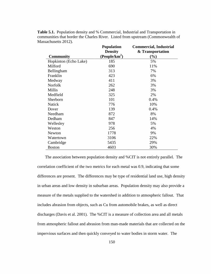
150

Table 5.1. Population density and % Commercial, Industrial and Transportation in

communities that border the Charles River. Listed from upstream (Commonwealth of

Massachusetts 2012).

Population

Density

Commercial, Industrial

& Transportation

Community (People/km2) (%)

Hopkinton (Echo Lake) 185 5%

Milford 690 11%

Bellingham 313 7%

Franklin 423 6%

Medway 411 3%

Norfolk 262 3%

Millis 248 3%

Medfield 325 2%

Sherborn 101 0.4%

Natick 776 10%

Dover 139 0.4%

Needham 872 8%

Dedham 847 14%

Wellesley 978 5%

Weston 256 4%

Newton 1778 9%

Watertown 3106 22%

Cambridge 5435 29%

Boston 4603 30%

The association between population density and %CIT is not entirely parallel. The

correlation coefficient of the two metrics for each metal was 0.9, indicating that some

differences are present. The differences may be type of residential land use, high density

in urban areas and low density in suburban areas. Population density may also provide a

measure of the metals supplied to the watershed in addition to atmospheric fallout. That

includes abrasion from objects, such as Cu from automobile brakes, as well as direct

discharges (Davis et al. 2001). The %CIT is a measure of collection area and all metals

from atmospheric fallout and abrasion from man-made materials that are collected on the

impervious surfaces and then quickly conveyed to water bodies in storm water. The

151

difference between the two metrics may be that parking lots and transportation networks

may displace population. This analysis examined the association of each of these

metrics.

The contribution of land use through the population density and %CIT may be

obscured by a number of anthropogenic sources and mechanisms. Echo Lake in

Hopkinton, Massachusetts is the headwaters of the Charles River and the background

location for the metal concentrations. It was determined in Chapter 3 that Echo Lake

metal concentrations were affected by storm water from residential areas. Additional

sources of increased concentrations of Cu, Zn, Pb, Hg and TOC downstream of Echo

Lake may include: the bedrock geology, industrial discharges, POTWs, historically-

contaminated sediments that are re-suspended, and storm water runoff from urban areas.

The bedrock geology is a source of natural metals. The contribution of the geology

at Echo Lake, representative of much of the Upper Charles River watershed, was

described in Chapter 3. There is a change of rock type in the Lower Charles River

watershed but that change is located just upstream of Watertown Dam, Station #13.

Therefore, it is unlikely that geology would be the source of increases in sediment metal

concentrations through Station #13.

Industrial discharges at Box Pond have contributed many metals to sediments in the

past (U.S. Environmental Protection Agency 1993; U.S. Environmental Protection

Agency 1997; Chi et al. 2009). During the period the surface sediment samples were

believed to be deposited in the Charles River, 1990 to 2000, industrial discharges were

regulated under State and Federal laws and therefore perhaps not a direct contributor to

152

sediment metal concentrations. Industries with metal-containing discharges had pre-

treatment programs at the facility that lowered the concentrations of waste streams prior

to discharge to sewage treatment plants or Publically-owned treatment works (POTWs)


Focusing on POTWs as potential sources, the Upper Charles River has three sewage

treatment plants in Milford, Medway and Medfield shown on Figure 5.1. The

communities below Medfield either have individual septic systems or are connected to

the Deer Island Facility on Boston Harbor and therefore do not contribute sewage directly

to the Charles River (Charles River Watershed Association 2005). The combined

average daily flow of all three treatment plants to the Charles River in 1998 was 42

million liters per day or approximately 0.5 m3 s

-1 (Charles River Watershed Association

2000). The Milford POTW is a tertiary treatment plant that treats and discharges

residential and industrial sewage to the Charles River.

Another potential source of metals to waterways and sediments are deposits of

historically-contaminated sediments that are re-suspended (Simpson et al. 1998). The

concentrations of several metals in surface sediments of Box Pond are elevated above

regulatory guidelines for aquatic life in sediments, especially Hg (Ingersoll et al. 1996;

U.S. Department of Commerce 2012). In Chapter 4, it was determined that relict

sediments, perhaps containing metals from a woolen mill abandoned in the mid-19th

century or metals from paint manufacturing, may be the source of continued high

concentrations of metals in the upper 3 cm of Box Pond sediments. High concentrations

of Hg, Zn and Pb and some portion of the Cu in sediments that post-date 1970 are

153

believed to be due to historic sediments that were eroded from upstream locations

contaminated by the paint industry.

Another source of metals, only recognized in the past 20 years, is storm water

runoff. As described in Chapter 1, storm water conveys metals from natural sources,

atmospheric fallout, and abrasion of man-made surfaces. Impervious areas collect

atmospheric fallout and direct it to waterways where the metals may be incorporated into

sediments (Van Metre and Mahler 2003; Wallace et al. 2004). The population density

and %CIT were examined with respect to the concentrations of metals in sediment. This

relationship was found to be significant in Chapter 3 for the Echo Lake watershed, and

has been shown to be relevant in other watersheds (Coles et al. 2004; Chalmers et al.

2007).

5.1.3. Sample Collection

Sediment collection occurred during three periods: sediment cores were collected

from Echo Lake in August 1999 and Box Pond in January 2001, and eleven sediment

surface samples were collected in June 2001. The upper 3 cm of the sediments were

examined based on sediment core dates from Echo Lake and Box Pond, two of the 13

stations, using radionuclide techniques. The general goal was to examine the previous 10

years of deposition, 1990 to 2000, because environmental regulations should have

reduced or eliminated direct discharges, and therefore improvements in water quality and

hence, sediment quality, were expected. The upper 3 cm of the Echo Lake and Box Pond

sediment cores were dated at 21 and 30 years of sediment, respectively (Luce and

154

Wallace, in preparation). The Box Pond location was similar to the other 11 locations

and therefore that value was selected.

The concentrations of the metals and TOC in the upper 3 cm of the sediment cores

from Echo Lake and Box Pond, described in Chapters 3 and 4, respectively, were

averaged to supply a single value for these locations and serve as representative surface

sediment samples. The eleven sediment surface samples were collected at locations

selected on the basis of having the least potential for local road runoff and other recent

disturbances.

Ten of the eleven surface sediment sampling locations were selected to obtain a fine-

grained sample from the upper 3 cm of sediment from that location. A coarse-grained

surface sediment, believed to have a low total organic carbon (TOC) content, was

collected at the background location, Echo Lake. Metal binding is associated with the

concentration of TOC in sediments (Mantoura et al. 1978; DiToro 2001). Obtaining both

high and low TOC sediments from the background location facilitated comparison to

sediment further downstream that may have low TOC concentrations.

Sediment cores of 9 and 12 cm were collected at two stations that had fine grained

sediments and were located near points that may show long-term trends of deposition.

Sediments were sectioned at 3 cm intervals in the eleven surface samples unless there

was a composition change in the sediment and in which case the section was shortened to

collect only that stratum. The sample stations were designated by the distance upstream

from the Charles River dam. For instance, the Echo Lake core was taken approximately

125 km upstream of the Charles River dam and is thus named Station #125.

155

The thirteen total sediment stations beginning at the headwaters of the Charles River,

and proceeding downstream, are described below as to conditions and pertinent features.

Echo Lake is a protected drinking water reservoir and the two sediment samples taken at

this location are considered the background, affected primarily by atmospheric

deposition. A coarse-grained low TOC sediment sample was collected near the bank of

Echo Lake, Station #125.1, and a sediment core, containing fine-grained sediment, was

collected at the deepest portion of the lake, Station #125.

Downstream of Echo Lake, the Charles River passes Milford, Massachusetts, a large

urban and industrial area that has been active since the 19th

century. The water that was

taken from Echo Lake is returned to the Charles River a short distance downstream from

Milford, after treatment, by the Milford POTW. A sediment core was collected

downstream of Milford and the Milford POTW, at an impoundment on the Charles River,

Box Pond, Station #111, to assess the impact of an urban, industrial watershed on the

concentrations of metals and TOC. Similar to Station 125, the concentrations of metals

and TOC in sediments for Station #111 are an average of sediment concentrations over 3

cm.

After Box Pond, the Charles River flows approximately 60 km through an area that

has a lower population density and lower %CIT. Within this run of the river are Stations

#95, #70, #53, #52.9. The sampling locations at Stations #95, #70, which are Walker

Street and Bridge Street, respectively, are not behind dams, but are in narrow channels

with coarser sediments. These stations are a short distance downstream of POTWs in

Medway and Medfield, Massachusetts, respectively.

156

Sediment samples were collected from a near-shore area above Cocharan Dam,

Station #53, and above the USGS gauging station, Station #52.9, which was a concrete

weir across the river. The samples from these four locations, Stations #95, #70, #53 and

#52.9, were selected to represent a stretch of the river flowing through a rural area with a

population density below 400 people km-2

.

The character of the river changes at the Ames Street sampling point, Station #42.

Upstream of Station #42 urban areas become more prevalent and the population density

increases to over 800 people km-2

(Commonwealth of Massachusetts 2012). Through

this area the Charles River widens and flows more slowly. At Station #41 there is a

structure that is used to attenuate flooding by diverting water into the Neponset River

watershed, hence this station is designated “Neponset River.” A 9 cm core was collected

at this location and sectioned at 3 cm intervals to determine if changes had occurred over

time due to the proximity of a major roadway, Route 1. The 9 cm core would indicate

any trends, potentially over 30 years.

The area of Stations #23 and #22.4 is an impoundment and no flow was evident.

The population density decreases in this area primarily due to the intersection of a major

transportation network, Interstate Routes 90 and 95 meet upstream of this area. Route 90

is a turnpike with additional impervious associated with the toll plazas and interchanges.

The increase in transportation network greatly increases the amount of storm water issued

to the river in this area.

At Station #23, the Charles River Watershed Association (CRWA) maintains a

recreational area with a dock and boat rental. The sediment sample at Station #23 was

157

obtained with a Ponar grab sample device operated from the dock. A 12 cm core was

collected at Station #23 and sectioned at 3 cm intervals to assess the long-term effects of

storm water from the roadways. Station # 22.4 was taken from the bank of the Charles

River approximately 0.6 km downstream of the CRWA dock to further gauge the effect

of storm water runoff from the highway system in a location less likely to be disturbed by

boat traffic.

The sediment sample obtained at the Watertown Dam, Station #13, was taken

approximately 100 m upstream of the dam. At the time of collection, the river was

flowing rapidly through this area and over the dam. The current slowed in the sample

area due to trees and debris deposited just upstream. It is likely that these sediments may

be younger than 10 years. The watershed surrounding the Charles River at Station #13 is

highly urban with a population density greater than 2,000 people km-2

(Commonwealth

of Massachusetts 2012).

Once the river flows over Watertown Dam the river enters the CRB, the standing

pool of water held back by the dam at Boston Harbor, 13 km further downstream. During

periods of low flow in the summer, a saline wedge has been known to penetrate as far as

the Watertown Dam from Boston Harbor (Breault et al. 2000). The last downstream

sampling point was in the CRB, off the dock at Elliott Bridge, Station #9. The area

surrounding Station #9 is highly urban. It is likely that the sediments in this area are

frequently disturbed by boat traffic and may be periodically affected by saline conditions.

The locations of the sampling points, with respect to latitude and longitude, are listed

in Table II.10 in Appendix II. The sample processing and analysis, as well as quality

158

assurance and quality control, are described in Chapter 2. Briefly, the concentrations of

Cu, Pb and Zn were determined with a Perkin-Elmer Inductively Coupled Plasma – Mass

Spectrometer, the concentration of Hg was determined by Cold Vapor Atomic

Adsorption, and TOC was determined with a Perkin-Elmer 2400 CHN analyzer.

159

5.2. Results and Discussion

The results of analysis for Cu, Zn, Pb, Hg and TOC are shown below in Table 5.2.

Table 5.2: Surface sediment concentrations of Cu, Zn, Pb , Hg and TOC from the

Charles River.

Station Strata Depth Cu Zn Pb Hg TOC

Station (km)1 Type

2 (cm) (µg/g) (µg/g) (µg/g) (ng/g) %

Echo Lake3 125 Muck 0-3 58 188 125 182 7.1

Echo Lake 125.1 Sand 0-3 8 39 26 209 1.0

Box Pond3 111 Muck 0-3 400 471 188 1471 13.0

Walker St 95 Silt

Sand

0-2 68 184 79 73 2.4

2 – 5 16 146 67 94 1.9

Bridge St –

Sherborn 70 Gravel 0-3 43 185 53 133 2.6

Cocharan

Dam 53

Fine

sand 0-3 22 154 76 176 3.0

USGS

station 52.9 Sand 0-3 7 63 19 33 0.6

Ames Street 42 Muck 0 – 3 78 544 131 387 8.9

3 – 6 85 376 120 385 10.0

Neponset

River 41 Silt

0 – 3 17 92 58 157 8.8

3 – 6 13 83 16 126 20.0

6 – 9 17 163 5 198 27.0

CRWA 23 Muck

0 – 3 104 696 283 678 13.2

3 – 6 103 695 284 650 9.8

6 – 9 105 662 343 738 9.3

9 – 12 109 672 426 1150 9.6

CRWA 22.4 Silt 0-3 84 645 251 896 10.7

Watertown

Dam 13 Silt 0-3 72 308 244 323 1.6

Elliott

Bridge 9

Silt 0 – 2 44 432 171 253 2.8

Clay 2 – 6 11 92 21 138 2.1 1 The distance (km) of the sampling station upstream from the dam separating the Charles River Basin

from Boston Harbor. 2 The designation of the type of material was based on observation of the collected material. Muck had no

observable particles. Silt had observable particles on smearing. 3 The Echo Lake (Muck) and Box Pond samples are the average concentrations of the upper 3 cm

determined from the sediment cores analyzed at 5 mm intervals.

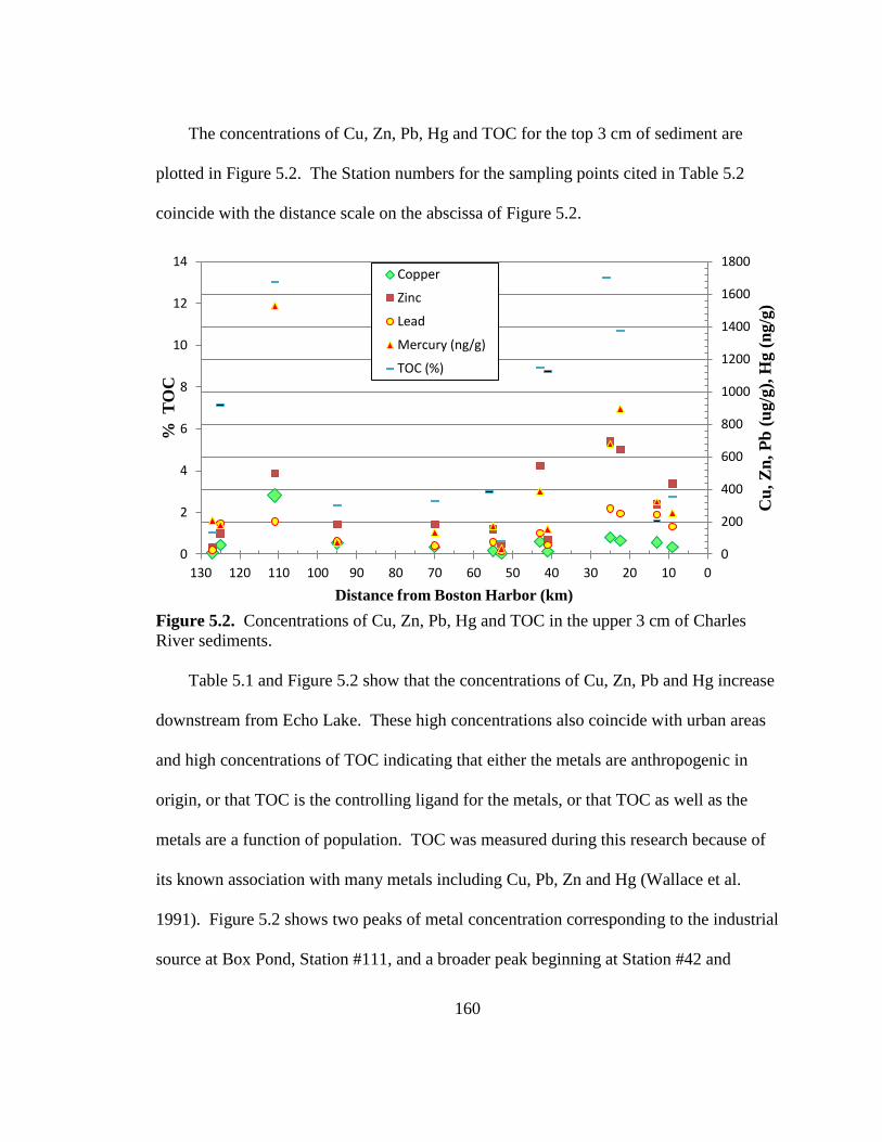
160

The concentrations of Cu, Zn, Pb, Hg and TOC for the top 3 cm of sediment are

plotted in Figure 5.2. The Station numbers for the sampling points cited in Table 5.2

coincide with the distance scale on the abscissa of Figure 5.2.

Figure 5.2. Concentrations of Cu, Zn, Pb, Hg and TOC in the upper 3 cm of Charles

River sediments.

Table 5.1 and Figure 5.2 show that the concentrations of Cu, Zn, Pb and Hg increase

downstream from Echo Lake. These high concentrations also coincide with urban areas

and high concentrations of TOC indicating that either the metals are anthropogenic in

origin, or that TOC is the controlling ligand for the metals, or that TOC as well as the

metals are a function of population. TOC was measured during this research because of

its known association with many metals including Cu, Pb, Zn and Hg (Wallace et al.

1991). Figure 5.2 shows two peaks of metal concentration corresponding to the industrial

source at Box Pond, Station #111, and a broader peak beginning at Station #42 and

0

2

4

6

8

10

12

14

0

200

400

600

800

1000

1200

1400

1600

1800

0 10 20 30 40 50 60 70 80 90 100 110 120 130

% T

OC

Cu

, Z

n, P

b (

ug

/g),

Hg (

ng/g

)

Distance from Boston Harbor (km)

Copper

Zinc

Lead

Mercury (ng/g)

TOC (%)

161

continuing to Station #22.4. The concentrations of metals in sediment decline in the two

stations downstream of Station #22.4, which is an area of intense urbanization. The

relationship between the concentrations of each of the metals, TOC, and land use metrics

is better examined on an individual basis.

5.2.1. Copper in the Charles River

An examination of the concentrations of Cu in the Charles River finds generally low

concentrations in sediments, except for Box Pond. Compared to other urban rivers, Cu

concentrations in Charles River sediments are higher in concentration. The National

Water Quality Assessment (NAWQA) determined that the median concentration for Cu

in 34 other urban waterways was 48 µg g-1

with upper and lower quartile values of 85 and

35 µg g-1

, respectively (Breault et al. 2000; Mahler et al. 2006). Table 5.2 and Figure 5.2

show that downstream of Box Pond (#111) sediment sample concentrations of Cu

decrease and, at stations #70, #53, and #52.9, are comparable to the background

concentration. The concentration of Cu in Charles River sediments begins to rise with

the increase in population density and %CIT land use, especially at Station #23 near a

major transportation network.

The linear regression of Cu with TOC concentration found an association (R2 =

0.38). Because TOC is an important ligand binding some metals, the Cu concentrations

were normalized by dividing the concentration of Cu in sediment by the TOC present.

The results were then compared to the population density and the %CIT in the

communities that border the Charles River as shown in Figure 5.3.

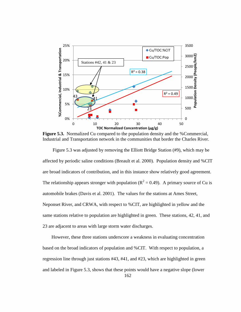
162

Figure 5.3. Normalized Cu compared to the population density and the %Commercial,

Industrial and Transportation network in the communities that border the Charles River.

Figure 5.3 was adjusted by removing the Elliott Bridge Station (#9), which may be

affected by periodic saline conditions (Breault et al. 2000). Population density and %CIT

are broad indicators of contribution, and in this instance show relatively good agreement.

The relationship appears stronger with population (R2 = 0.49). A primary source of Cu is

automobile brakes (Davis et al. 2001). The values for the stations at Ames Street,

Neponset River, and CRWA, with respect to %CIT, are highlighted in yellow and the

same stations relative to population are highlighted in green. These stations, 42, 41, and

23 are adjacent to areas with large storm water discharges.

However, these three stations underscore a weakness in evaluating concentration

based on the broad indicators of population and %CIT. With respect to population, a

regression line through just stations #43, #41, and #23, which are highlighted in green

and labeled in Figure 5.3, shows that these points would have a negative slope (lower

R² = 0.38

R² = 0.49

0

500

1000

1500

2000

2500

3000

3500

0%

5%

10%

15%

20%

25%

0 10 20 30 40 50

Po

pu

lati

on

De

nsi

ty (

Pe

op

le/k

m2

)

%C

om

me

rcia

l, In

du

stri

al &

Tra

nsp

ort

atio

n

TOC Normalized Concentration (µg/g)

Cu/TOC:%CIT

Cu/TOC:Pop

41

23

43

Stations #42, 41 & 23

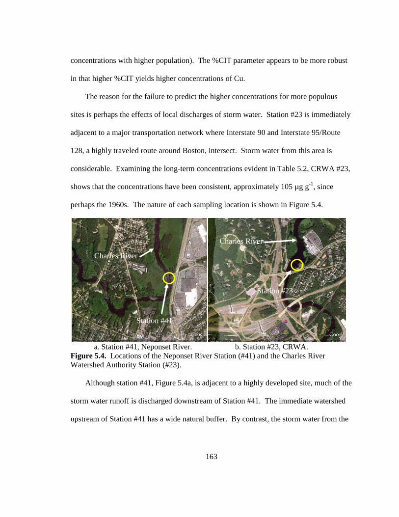
163

concentrations with higher population). The %CIT parameter appears to be more robust

in that higher %CIT yields higher concentrations of Cu.

The reason for the failure to predict the higher concentrations for more populous

sites is perhaps the effects of local discharges of storm water. Station #23 is immediately

adjacent to a major transportation network where Interstate 90 and Interstate 95/Route

128, a highly traveled route around Boston, intersect. Storm water from this area is

considerable. Examining the long-term concentrations evident in Table 5.2, CRWA #23,

shows that the concentrations have been consistent, approximately 105 µg g-1

, since

perhaps the 1960s. The nature of each sampling location is shown in Figure 5.4.

a. Station #41, Neponset River. b. Station #23, CRWA.

Figure 5.4. Locations of the Neponset River Station (#41) and the Charles River

Watershed Authority Station (#23).

Although station #41, Figure 5.4a, is adjacent to a highly developed site, much of the

storm water runoff is discharged downstream of Station #41. The immediate watershed

upstream of Station #41 has a wide natural buffer. By contrast, the storm water from the

Charles River

Charles River

Station #41

Station #23

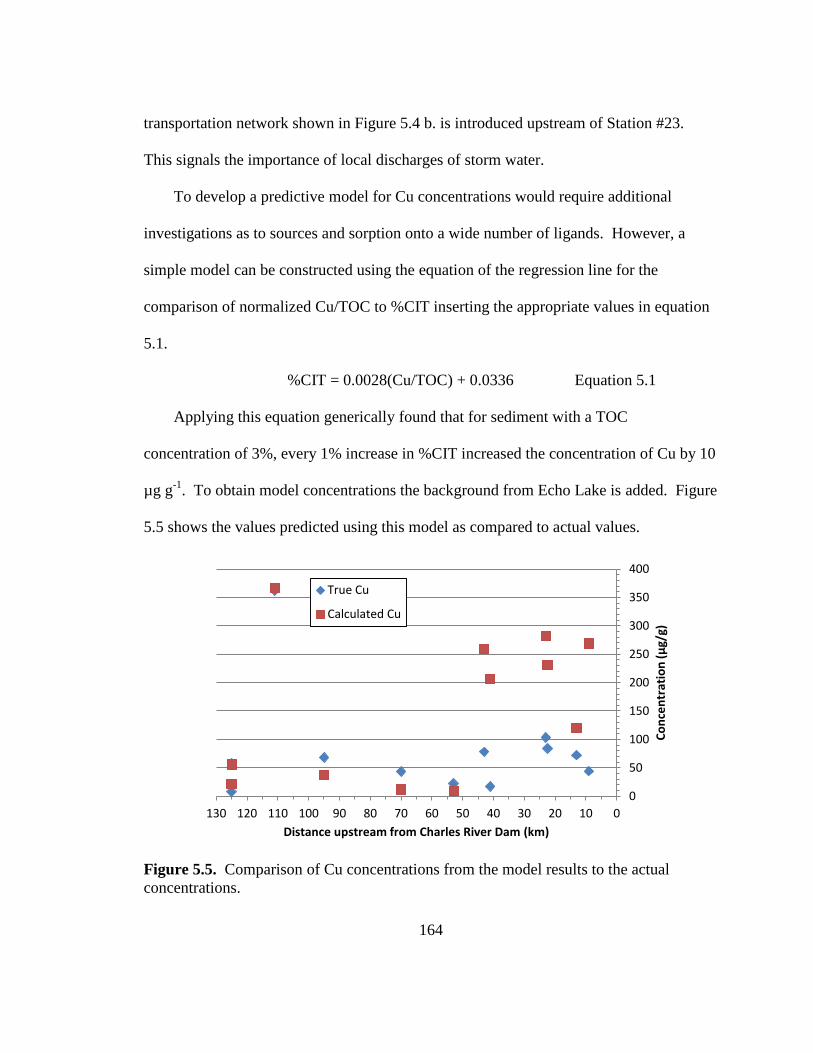
164

transportation network shown in Figure 5.4 b. is introduced upstream of Station #23.

This signals the importance of local discharges of storm water.

To develop a predictive model for Cu concentrations would require additional

investigations as to sources and sorption onto a wide number of ligands. However, a

simple model can be constructed using the equation of the regression line for the

comparison of normalized Cu/TOC to %CIT inserting the appropriate values in equation

5.1.

%CIT = 0.0028(Cu/TOC) + 0.0336 Equation 5.1

Applying this equation generically found that for sediment with a TOC

concentration of 3%, every 1% increase in %CIT increased the concentration of Cu by 10

µg g-1

. To obtain model concentrations the background from Echo Lake is added. Figure

5.5 shows the values predicted using this model as compared to actual values.

Figure 5.5. Comparison of Cu concentrations from the model results to the actual

concentrations.

0

50

100

150

200

250

300

350

400

0 10 20 30 40 50 60 70 80 90 100 110 120 130

Co

nce

ntr

atio

n (

µg/

g)

Distance upstream from Charles River Dam (km)

True Cu

Calculated Cu

165

Figure 5.5 shows good agreement (a correlation coefficient of 0.65) with stations in

the upper portion of the watershed. The model over-predicts in the lower stations

indicating that perhaps the association with Cu is non-linear or that other factors are

critical in binding Cu to sediment. Based on TOC and %CIT the sediments below Station

#42 are shown to be under-saturated with respect to Cu by this simple model.

5.2.2. Zinc in the Charles River

The concentrations of Zn shown in Table 5.2 and Figure 5.2 are much greater than

Cu with 6 of the 13 stations exceeding the NAWQA median value of 200 µg g-1

. The

average concentration of Zn in all surface sediments (137 µg g-1

) exceeds the ERL

concentration of 110 µg g-1

.

The correlation of Zn to TOC was better than Cu (R2 = 0.51), but the regression of

Zn normalized to TOC against either the %CIT or population density had a negative

correlation and a poor R2 (< 0.2) for each regression as well. The disagreement of the

TOC normalized Zn may be due to the nature of the particulate Zn. If the source of Zn is

tire wear as described in literature, it is possible that the TOC is ineffective as a measure

of Zn and another factor such as grain size becomes important (Davis et al. 2001).

Instead, the surface concentrations in Table 5.2 were plotted relative to the %CIT and

population density in Figure 5.6 instead of TOC normalized values.

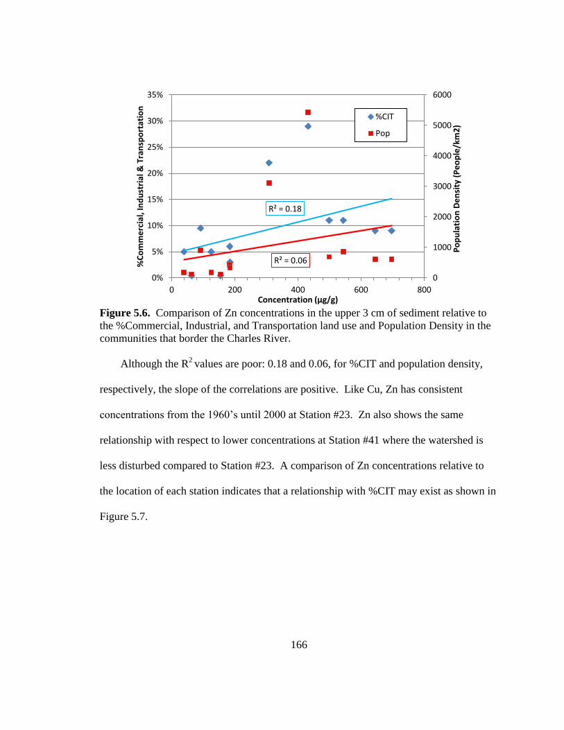
166

Figure 5.6. Comparison of Zn concentrations in the upper 3 cm of sediment relative to

the %Commercial, Industrial, and Transportation land use and Population Density in the

communities that border the Charles River.

Although the R2

values are poor: 0.18 and 0.06, for %CIT and population density,

respectively, the slope of the correlations are positive. Like Cu, Zn has consistent

concentrations from the 1960’s until 2000 at Station #23. Zn also shows the same

relationship with respect to lower concentrations at Station #41 where the watershed is

less disturbed compared to Station #23. A comparison of Zn concentrations relative to

the location of each station indicates that a relationship with %CIT may exist as shown in

Figure 5.7.

R² = 0.18

R² = 0.06

0

1000

2000

3000

4000

5000

6000

0%

5%

10%

15%

20%

25%

30%

35%

0 200 400 600 800

Po

pu

lati

on

De

nsi

ty (

Pe

op

le/k

m2

)

%C

om

me

rcia

l, In

du

stri

al &

Tra

nsp

ort

atio

n

Concentration (µg/g)

%CIT

Pop

167

Figure 5.7. Concentration of Zn in Charles River sediment is compared to the %

Commercial, Industrial and Transportation network of the communities that border the

river.

Figure 5.7 demonstrates parallels between %CIT and the concentration of Zn. The

%CIT is shown as a continuous line although it is recognized that the effects are more

likely to be more pronounced at the discharge points and trend to the average further

downstream from each discharge point. The correlation of Zn concentrations with %CIT,

the better result between %CIT and population density, yielded a correlation coefficient

of 0.42, but eliminating stations #13 and #9 improved the coefficient to 0.68. Station #13

is Watertown Dam, the flow of water at the time of collection was vigorous, TOC was

just 1.6% and it is possible that either the grain-size or the potentially younger age of the

sediments at Station #13 create the difference between Zn and %CIT. Station #9 was

eliminated due to the periodic saline influence. The relationship improved on a spatial

scale rather than a linear scale in the regression perhaps because the relationship is not

0%

5%

10%

15%

20%

25%

30%

35%

0

100

200

300

400

500

600

700

800

0 10 20 30 40 50 60 70 80 90 100 110 120 130

% C

om

me

rcia

l, In

du

stri

al a

nd

Tra

nsp

ort

atio

n

Co

nce

ntr

atio

n Z

n (

µg/

g)

Distance Upstream from Charles River Dam

Zn

%CIT

168

linear, that particle density or grain size is an important factor in Zn concentration which

would require focused investigation into the nature of the Zn particles and binding (Coles

et al. 2004). The simple model shown to work for Cu does not work with Zn. Applying

the same form of equation to the %CIT and %TOC did yield synthetic values that had a

high correlation coefficient (0.81). The regression and the modeled concentrations are

shown in Figure 5.8.

169

Figure 5.8. Association of Zn concentrations, normalized to TOC, with % Commercial,

Industrial and Transportation land use (upper graph) and the modeled results from that

association (lower graph).

A problem with this result is that the regression coefficient is greatly improved by

two outliers that if removed, yield a negative slope and poor regression coefficient.

Therefore, although Zn concentrations appear to be associated with %CIT in the Charles

River based on TOC, the confidence in that association is weak. Other factors that

y = 0.001035x + 0.018376 R² = 0.442964

0%

5%

10%

15%

20%

25%

30%

35%

0 50 100 150 200 250

%C

om

me

rcia

l, In

du

stri

al &

Tr

ansp

ort

atio

n

TOC Normalized Concentration (µg/g)

0 100 200 300 400 500 600 700 800 900 1000 1100 1200 1300 1400 1500

0 10 20 30 40 50 60 70 80 90 100 110 120 130

Co

nce

ntr

atio

n (

µg/

g)


True Zn

Calculated Zn

170

govern the concentration of Zn, principally grain size and sorption, must be examined

more closely to build a better model.

5.2.3. Lead in the Charles River

The concentration of Pb throughout the Charles River is pervasive. It exceeds the

ERL in all but three stations and the ERM in 7 of the 13 stations. Its average

concentration, 137 µg g-1

, exceeds the ERM and the upper quartile concentration for the

NAWQA water bodies (130 µg g-1

).

A comparison of the high TOC and low TOC Echo Lake Pb concentrations indicates

a dependence on TOC concentration. Yet the regression of Pb through the entire Charles

River against TOC values found the lowest R2 (0.38) of all four metals. Comparing the

concentrations of Pb normalized to TOC found consistently poor regression coefficients

indicating that Pb shared the character of Zn in that other factors were important to the

concentration of Pb relative to land use as expressed by %CIT. In Figure 5.9 the

concentration of Pb is plotted relative to the Station location.

171

Figure 5.9. Concentration of Pb at each of the sampling stations compared to the

%Commercial, Industrial, and Transportation land use in communities that border the

Charles River.

Figure 5.9 shows a similar pattern to that of Zn, the correlation coefficient for Pb

sediment concentration relative to %CIT was 0.51. The high concentration of Pb at

Station #125 compared to downstream stations was unexpected, but may be due to the

ratio of open water to the watershed and the presence of municipal trash incineration

nearby (Massachusetts Department of Environmental Protection 2011). The open water

of Echo Lake comprises 10% of its watershed while open water in the entire Charles

River watershed is 2.6%. The Pb that is delivered through the atmosphere may be

incorporated into the Echo Lake sediments with less attenuation from soils and other

materials in the watershed than the remaining river.

If the direct fallout of Pb onto open water at Echo Lake is the difference, this

indicates that watershed soils are an important surface in absorbing and increasing the

0%

5%

10%

15%

20%

25%

30%

35%

0

50

100

150

200

250

300

0 10 20 30 40 50 60 70 80 90 100 110 120 130

% C

om

me

rcia

l, In

du

stri

al a

nd

Tra

nsp

ort

atio

n

Co

nce

ntr

atio

n P

b (

µg/

g)


Pb

%CIT

172

residence time of Pb in the watershed soils, delaying the increase in sediments. The

importance of this attenuation factor is shown by the rise in concentration beginning at

Station #23 where storm water from a major highway network enters the river.

Station #23 is greatly affected by the nearby interstate system. Table 5.2 also shows

that the lower 3 cm horizons collected at Station #23 parallel the lowering in

concentration of Pb due to the leaded gas ban, with the lowest interval (9 to 12 cm deep)

nearly twice the value (426 µg g-1

) than the top 3 cm (283 µg g-1

).

Attempts to obtain a predictive model similar to Cu did not work for Pb for the same

reasons they did not work for Zn. The regression of Pb normalized to TOC against the

%CIT was affected by two outliers which, if removed yield a negative correlation. This

indicates that the concentration of Pb is dependent on factors that govern its sorption and

perhaps the proximity of any discharges. The modeled results did show fair agreement

for some of the stations in the upper watershed, but no agreement for Stations #42, #41,

#23, and #22.4. Figure 5.10 compares the modeled to the true concentrations of Pb in the

Charles River.

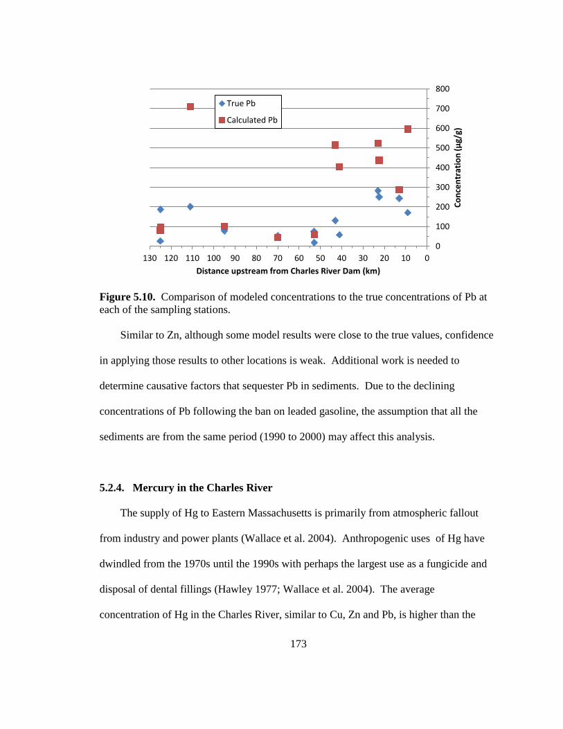
173

Figure 5.10. Comparison of modeled concentrations to the true concentrations of Pb at

each of the sampling stations.

Similar to Zn, although some model results were close to the true values, confidence

in applying those results to other locations is weak. Additional work is needed to

determine causative factors that sequester Pb in sediments. Due to the declining

concentrations of Pb following the ban on leaded gasoline, the assumption that all the

sediments are from the same period (1990 to 2000) may affect this analysis.

5.2.4. Mercury in the Charles River

The supply of Hg to Eastern Massachusetts is primarily from atmospheric fallout

from industry and power plants (Wallace et al. 2004). Anthropogenic uses of Hg have

dwindled from the 1970s until the 1990s with perhaps the largest use as a fungicide and

disposal of dental fillings (Hawley 1977; Wallace et al. 2004). The average

concentration of Hg in the Charles River, similar to Cu, Zn and Pb, is higher than the

0

100

200

300

400

500

600

700

800

0 10 20 30 40 50 60 70 80 90 100 110 120 130

Co

nce

ntr

atio

n (

µg/

g)


True Pb

Calculated Pb

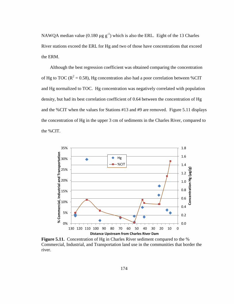
174

NAWQA median value (0.180 µg g-1

) which is also the ERL. Eight of the 13 Charles

River stations exceed the ERL for Hg and two of those have concentrations that exceed

the ERM.

Although the best regression coefficient was obtained comparing the concentration

of Hg to TOC (R2 = 0.58), Hg concentration also had a poor correlation between %CIT

and Hg normalized to TOC. Hg concentration was negatively correlated with population

density, but had its best correlation coefficient of 0.64 between the concentration of Hg

and the %CIT when the values for Stations #13 and #9 are removed. Figure 5.11 displays

the concentration of Hg in the upper 3 cm of sediments in the Charles River, compared to

the %CIT.

Figure 5.11. Concentration of Hg in Charles River sediment compared to the %

Commercial, Industrial, and Transportation land use in the communities that border the

river.

0%

5%

10%

15%

20%

25%

30%

35%

0.0

0.2

0.4

0.6

0.8

1.0

1.2

1.4

1.6

1.8

0 10 20 30 40 50 60 70 80 90 100 110 120 130

% C

om

me

rcia

l, In

du

stri

al a

nd

Tra

nsp

ort

atio

n

Co

nce

ntr

atio

n H

g (µ

g/g)


Hg

%CIT

175

The Hg concentration at Station #111 is likely due to the erosion of sediments

tainted by disposal of Hg in the paint manufacturing process that may have lasted until

1991 (Hawley 1977; U.S. Environmental Protection Agency 2012). Examining the

results of Station #23 in Table 5.2 finds higher concentrations in deeper, older sediments.

Concentrations in the sediment column taken at Station #41 are much lower than even the

present concentrations at Station #23. Both Pb and Hg are highly regulated metals in

industry and both metals have been slowly eliminated from regular consumer use since

the mid-1970’s (Chillrud et al. 1999; U.S. Environmental Protection Agency 2012).

Because the top 3 cm are estimated to have been deposited since 1990, it would be

expected that concentrations of Pb and Hg would be restricted to atmospheric fallout

(Van Metre and Mahler 2003; Wallace et al. 2004). Because the concentration of Hg is

low at Station #41 while downstream at Station #23 it is elevated it must be assumed that

the source is atmospheric fallout.

Although the regression value was poor (R2 = 0.15), the association of TOC

normalized Hg to %CIT appeared to not be affected by outliers. Similar to Cu, a simple

model was constructed using the equation of the regression line for the comparison of

normalized Hg/TOC to %CIT inserting the appropriate values in equation 5.2 and adding

the background concentration developed in Chapter 3 for Echo Lake, 0.115 µg g-1

.

%CIT = 0.5072(Hg/TOC) + 0.0523 Equation 5.2

Applying this equation found that for sediment with a TOC concentration of 3%,

every 1% increase in %CIT increased the concentration of Hg by approximately 0.060 µg

g-1

. Figure 5.12 shows the values predicted using this model compared to actual values.

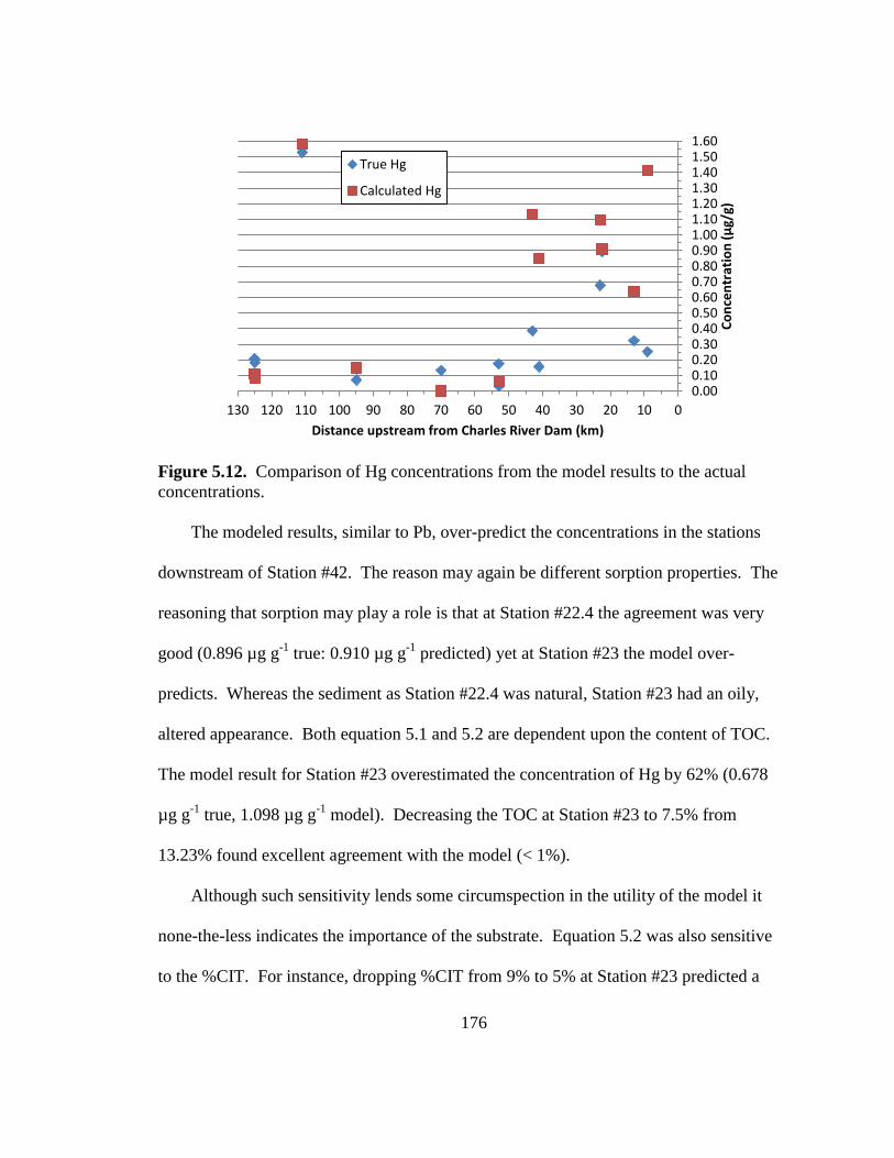
176

Figure 5.12. Comparison of Hg concentrations from the model results to the actual

concentrations.

The modeled results, similar to Pb, over-predict the concentrations in the stations

downstream of Station #42. The reason may again be different sorption properties. The

reasoning that sorption may play a role is that at Station #22.4 the agreement was very

good (0.896 µg g-1

true: 0.910 µg g-1

predicted) yet at Station #23 the model over-

predicts. Whereas the sediment as Station #22.4 was natural, Station #23 had an oily,

altered appearance. Both equation 5.1 and 5.2 are dependent upon the content of TOC.

The model result for Station #23 overestimated the concentration of Hg by 62% (0.678

µg g-1

true, 1.098 µg g-1

model). Decreasing the TOC at Station #23 to 7.5% from

13.23% found excellent agreement with the model (< 1%).

Although such sensitivity lends some circumspection in the utility of the model it

none-the-less indicates the importance of the substrate. Equation 5.2 was also sensitive

to the %CIT. For instance, dropping %CIT from 9% to 5% at Station #23 predicted a

0.00 0.10 0.20 0.30 0.40 0.50 0.60 0.70 0.80 0.90 1.00 1.10 1.20 1.30 1.40 1.50 1.60

0 10 20 30 40 50 60 70 80 90 100 110 120 130

Co

nce

ntr

atio

n (

µg/

g)


True Hg

Calculated Hg

177

sediment concentration below the background concentration in Echo Lake. This

highlights either an inaccuracy in the model or that drainage improvements can have a

significant impact on metal concentrations. Regardless, for all the metals a greater

understanding of the processes that bind the metals to soils and sediment in the watershed

is necessary to resolve the differences found.

5.3 Toxicity, Trends and Implications of Metals in Sediments

The concentrations of Cu, Pb, Zn and Hg exceeded toxicity standards established by

regulatory agencies at many of the stations established in the Charles River. In fact, no

sediment sampling point was below the regulatory standards for all metals. Table 5.3

highlights the metals that exceed regulatory standards.

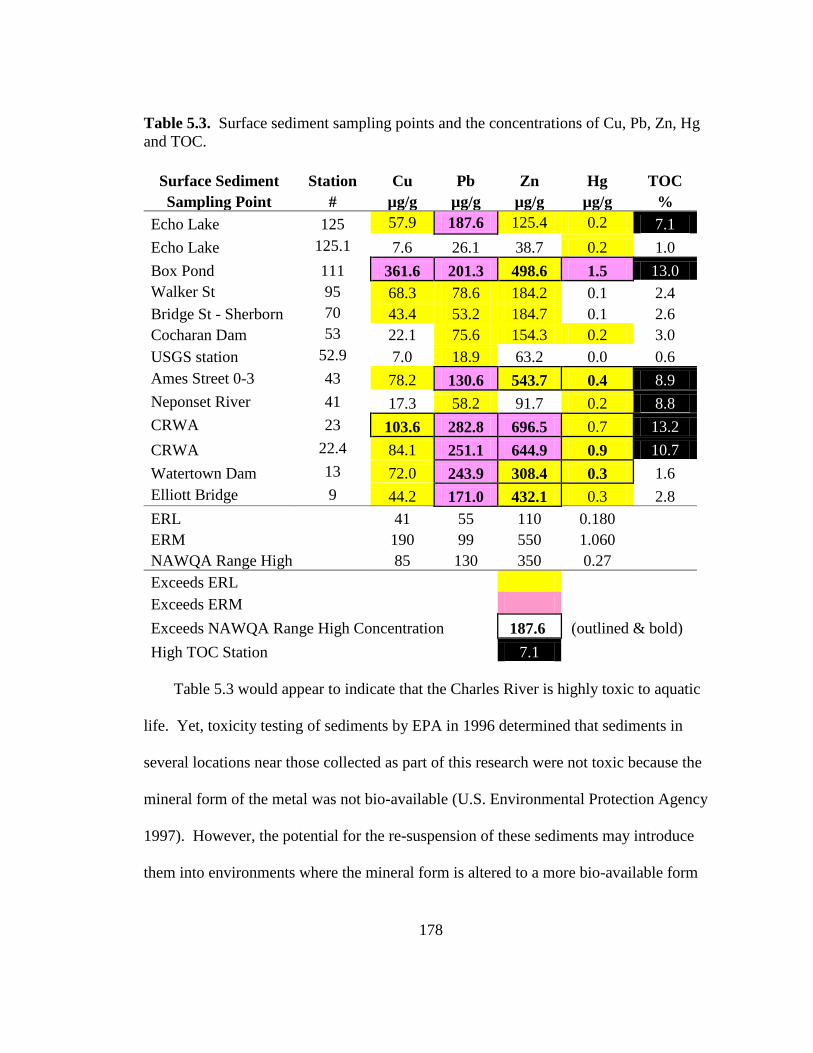
178

Table 5.3. Surface sediment sampling points and the concentrations of Cu, Pb, Zn, Hg

and TOC.

Surface Sediment Station Cu Pb Zn Hg TOC

Sampling Point # µg/g µg/g µg/g µg/g %

Echo Lake 125 57.9 187.6 125.4 0.2 7.1

Echo Lake 125.1 7.6 26.1 38.7 0.2 1.0

Box Pond 111 361.6 201.3 498.6 1.5 13.0

Walker St 95 68.3 78.6 184.2 0.1 2.4

Bridge St - Sherborn 70 43.4 53.2 184.7 0.1 2.6

Cocharan Dam 53 22.1 75.6 154.3 0.2 3.0

USGS station 52.9 7.0 18.9 63.2 0.0 0.6

Ames Street 0-3 43 78.2 130.6 543.7 0.4 8.9

Neponset River 41 17.3 58.2 91.7 0.2 8.8

CRWA 23 103.6 282.8 696.5 0.7 13.2

CRWA 22.4 84.1 251.1 644.9 0.9 10.7

Watertown Dam 13 72.0 243.9 308.4 0.3 1.6

Elliott Bridge 9 44.2 171.0 432.1 0.3 2.8

ERL 41 55 110 0.180

ERM 190 99 550 1.060

NAWQA Range High 85 130 350 0.27

Exceeds ERL

Exceeds ERM

Exceeds NAWQA Range High Concentration 187.6 (outlined & bold)

High TOC Station 7.1

Table 5.3 would appear to indicate that the Charles River is highly toxic to aquatic

life. Yet, toxicity testing of sediments by EPA in 1996 determined that sediments in

several locations near those collected as part of this research were not toxic because the

mineral form of the metal was not bio-available (U.S. Environmental Protection Agency

1997). However, the potential for the re-suspension of these sediments may introduce

them into environments where the mineral form is altered to a more bio-available form

179

and toxicity may occur (U.S. Environmental Protection Agency 1997; Rogers et al.

2002).

The presence of high concentrations of metals in the Charles River sediments can

pose hazards to aquatic life and present a future management problem. Determining the

sources of continued metal deposition to sediments must be considered in restoring the

river.

Although testing has found the high concentrations of metals in the Charles River do

not pose a threat of toxicity to test organisms, the paradigm of exposure of aquatic

organisms may have flaws. Other research has found that the fine veneer of sediments

associated with vegetation may create an environment where sediment metals were less

likely to be bound by sulfides and therefore more bio-available (Rogers et al. 2002). The

important aspect of the above, to this research, is that there exists a reservoir of sediments

in Box Pond and other downstream locations that contain metals that may be suspended

and create conditions downstream that are toxic to aquatic life and degrade water quality.

Since 1995 EPA has spent considerable amounts of money and effort to make the

Charles River safe for boating and swimming, with respect to bacterial counts, 100% of

the time. That goal was to be achieved by 2005, but has not yet been attained (U.S.

Environmental Protection Agency 2005). EPA has since addressed other parameters to

restore the general health of the river. One such effort is reducing phosphorus to

minimize blue-green algae blooms (U.S. Environmental Protection Agency 2008).

However, the approach taken thus far has not examined the interplay of sediments with

water quality. Excess metal concentrations have been shown to impact the diversity of

180

bacterial colonies (Singleton and Guthrie 1977). The sorption characteristics of the river

sediments may control the concentration of metals nearly as much as the inputs into the

river. Therefore, examining the behavior of metals and the sorption properties of

sediments in the Charles River may assist in its restoration.

Another consideration is that as many of the dams along the Charles River fill with

sediment, the need to manage or dispose of these sediments during dredging or dam

removal projects must be considered (Doyle et al. 2003). Many of the dams along the

Charles River are the remains of former mills and are therefore sometimes greater than

100 years old (McAdow 1992). For instance, the average depth of Box Pond was

estimated to be 1.5 meters in depth in January 2001. At a sedimentation rate of 0.3 cm

yr-1

, determined in Chapter 4, more than half the existing water column of Box Pond will

be lost by 2035 without dredging. Dredging may be conducted if conditions deteriorate

in the stream and sufficient money is available. If dredging occurs the sediment will

certainly contain high concentrations of metals and potentially other contaminants that

will require special handing in their disposal.

5.4 CONCLUSIONS

The concentrations of Cu, Zn, Pb, and Hg in Charles River sediments deposited in

the last ten years were determined to exceed the range of concentrations for those metals

in other, similar urban water bodies and exceed regulatory guidelines established to

assess toxicity to aquatic organisms in much of the river.

181

The concentrations of Cu, Zn, Pb and Hg were a function of both population density

and %CIT. The better associations were found with %CIT and, using TOC

concentrations, simple regression models were developed to predict Cu and Hg

concentrations in sediment. Disagreements between the modeled results and the actual

results appear to be a function of sorption characteristics. The association with %CIT

and the sensitivity of the model with respect to %CIT signals the importance of storm

water and its flow into surface waters such as the Charles River. The model indicates

that minimizing storm water runoff in the area of the intersection of Interstate Routes 90

and 95 may improve conditions in the Charles River.

182

CHAPTER 6

THE CHARLES RIVER, SUMMARY AND CONSIDERATIONS

Abstract

The analysis of dated sediment cores and surface sediment samples taken in the

Charles River found that changing land use in the Charles River watershed increased the

concentration of metals in sediments. Land use, measured as the percentage of

Commercial, Industrial and Transportation network, resulted in increases of storm water

flow which decreased the residence time of metals in the upland areas of the watershed.

The impoundments created along the river received these metals, sorbed to sediments,

and deposited them behind the dam thus increasing their residence time within the

Charles River. Simple models indicated that improvements in storm water management

may reduce the concentrations of metals that may cause toxicity in aquatic organisms.

Restoring the Charles River and other similar, urban rivers is desirable as these water

ways are increasingly used for recreation. To design cleanup efforts for urban rivers will

require different monitoring and analysis strategies to determine sediment inventories and

the present fluxes of metals into water ways. Understanding the sources and fluxes of

metals to the storm water is needed to restore the Charles River.

183

6.1 Introduction

The Charles River is a signature element of Boston, but historically was one of the

more polluted waterways in the nation (Breault et al. 2000; Haglund 2003). As such,

EPA and other regulatory agencies have been attempting to restore it for public use (Hill

1975; U.S. Environmental Protection Agency 2005).

The cleanup effort intensified in 1995 with creation of the Clean Charles 2005

program. The goal of the program was to make boating and swimming in the Charles

River Basin in Boston safe 100% of the time, with respect to surface water concentrations

of Escherichia coli bacteria, by 2005. In 1995, the first year of monitoring, the river was

safe for boating 39% and swimming 19% of the time. Steady progress occurred but

reached an asymptote short of that goal and as of 2009 the river was safe for boating 92%

and swimming 62% of the time (U.S. Environmental Protection Agency 2005).

EPA has worked to eliminate discharges to the Charles River, but has since

determined that other factors are partly responsible for the continued poor water quality.

EPA expanded efforts to achieve the 100% safe goal by increasing storm water

regulations and focusing on nutrients in the upper watershed to address cyanobacteria

(blue-green algae) (Tetra-Tech Inc. 2009; U.S. Environmental Protection Agency 2010;

U.S. Environmental Protection Agency 2011).

EPA’s assessment of the Charles River has been primarily through surface water

monitoring of a narrow range of parameters (U.S. Environmental Protection Agency

2005). Surface water sampling has utility, but provides only a snapshot of a dynamic

system and does not allow for a discrimination of contaminant sources. Determining the

184

sources of impairment and addressing them will allow a more efficient means of restoring

the river. Sediments are the primary substrate in contact with surface water and therefore

have the greatest capacity to affect long-term water quality (Boudreau and Jorgensen

2001; Ren and Packman 2004). Although there are few links between sediment quality

with respect to metals and microbial communities, some impairment of microbial

diversity due to high concentrations of metals has been demonstrated (Singleton and

Guthrie 1977). Metals may also influence the aquatic communities and water quality

(Luoma and Carter 1991; Peeters et al. 2000). Therefore, a more thorough

characterization of sediments may better address problems with water quality in the

Charles River.

Because of the particle-reactive nature of metals and their tendency to be incorporated

into sediments, sediments provide a means of assessing changes and trends of metal

concentrations in waterways (Olsen 1979; Olsen et al. 1982). Dated sediment cores

allow the connection of historical land use changes to changes in metal concentrations in

sediment.

This dissertation determined the concentration trends of metals in sediments with

respect to certain land uses. Chapters 3 and 4 discussed the analytical results of two

sediment cores collected in the headwaters of the Charles River. These chapters

described the effect of different land uses and sources, as well as the processes that

affected sediment metal concentrations. The land use types evaluated included

residential development, established urban areas, and industrial and commercial

activities. Chapter 5 extended the conclusions drawn from Chapters 3 and 4 and

185

determined relationships between land use and metal concentrations in sediments

throughout the river in a more limited time frame using surface sediments.

Because the Charles River and other rivers in urban areas are increasingly looked

upon as recreational resources, characterizing all components of a waterway become

important (Haglund 2003). A better understanding of the relationship between land use,

population density and the concentration of metals in sediments will enable more

effective regulation and management of discharges to all rivers.

Taken together, Chapters 3, 4, and 5 of this dissertation suggest new approaches to

monitoring and managing urban rivers. Sediment sampling, and in particular the analysis

of dated cores, is a missing component of the Charles River monitoring program.

Properly assessed, sediment cores can be used to set regulatory standards and plan

restoration efforts. Increased monitoring of other sources and discharges to the river to

determine the fluxes of metals and other contaminants can also clarify the sources of

impairment. This research can be used as a case study of the Charles River Watershed, a

typical urban watershed, to suggest the use of dated sediment cores in the assessment of

watershed health.

6.2 Sampling and Analysis

The samples for this dissertation consisted of two sediment cores and 11 surface

sediment grab samples. The sediment cores were collected in two impoundments on the

Charles River, Echo Lake and Box Pond, and were 35 and 30 cm in length, respectively.

Each sediment core was sectioned at 5 mm intervals and absolute dates were assigned to

186

those intervals through radiometric dating techniques using 210

Pb, 214

Pb and 137

Cs. The

surface sediment samples consisted of the upper 3 cm of sediment and were collected at

various intervals along the Charles River. The 5 mm sediment core intervals and the 3

cm thick surface sediment samples were processed and analyzed for TOC, Al, Fe, Mn,

Hg, Pb, Cd, Cu, Zn, Ag, Sc, Sr, As, Cd, Sn, Cr and Co. Techniques and quality assurance

and quality control are discussed in Chapter 2.

Weighing into each evaluation was consideration of the physical and chemical factors

that may affect metal concentration and deposition rates as those metals traverse the

watershed, enter the waterways and are then deposited. Physical factors considered

included alterations to waterways such as dams and storm water management. Chemical

factors included the addition of metals through atmospheric fallout, direct discharges, and

the concentration of TOC as well as the potential chemical changes imparted by the

physical changes listed in Chapter 1.

Federal and State agencies begin their assessment of sediment metal concentrations

based on their potential for toxicity. These guidelines include the Effects Range Low

(ERL) and Effects Range Median (ERM). Within this research seven of the analyzed

metals have established values to assess toxicity: Hg, Pb, Cd, As, Zn, Cu, and Cr. The

general application is that concentrations of these metals that are below the ERL rarely

exhibit toxicity, while concentrations exceeding the ERM usually have toxic effects and

additional sampling and other assessments are performed (Ingersoll et al. 1996; National

Oceanic and Atmospheric Administration 1999). In this dissertation the ERL and ERM

187

concentrations were used as a benchmark to evaluate the severity of metal contamination

and the importance of any concentration trends.

6.3 Echo Lake Sediment Core

Echo Lake, the headwaters of the Charles River, is a drinking water reservoir that has

been protected for more than 100 years. Yet, analysis of the Echo Lake sediment core

found metal concentrations increased by anthropogenic activities. Concentrations of Pb

and Hg determined in Echo Lake sediments deposited during the 19th

century

demonstrated the importance of atmospheric fallout. The concentrations of Pb from 1860

to 1880 were increased by emissions from an industrial area outside of the Echo Lake

watershed. Increases in Hg concentrations during three separate intervals: 1872, 1887 to

1889, and 1903, appeared to be the result of local atmospheric discharges during

construction of a railroad line and two dams. The concentrations of both metals in these

specific intervals of sediments exceed the modern-day ERL. This result not only

demonstrates the impact of atmospheric deposition, but also that older sediments are not

necessarily free of anthropogenic effects even in remote water bodies.

The Echo Lake watershed transitioned from a rural, undeveloped area, to a residential

area beginning in 1969. Atmospheric deposition remained an important source for metals

in Echo Lake sediments, but the residential development was also found to impact the

concentrations of metals in sediment despite a 500 m unaltered buffer zone surrounding

the lake.

188

Analysis of the Echo Lake sediment core determined that despite a 500 m buffer

zone, residential development in the watershed since 1970 had increased the

concentration of several metals to exceed regulatory standards for aquatic life and altered

the lake ecology. The deposition rate of sediments increased four-fold over natural

conditions after 1969, perhaps due to poor erosion control during construction of the

roadways for the subdivisions, and appears to be responsible for the elimination of rooted

aquatic plants in 1984 that had populated the lake bottom since 1882. The excess

sedimentation may have also increased the supply of other nutrients that created a bloom

of floating nuisance aquatic vegetation in 1990 that required treatment with copper

sulfate.

The source of anthropogenic Hg, Pb, and Cd in Echo Lake appears to be atmospheric

fallout that is collected by storm water and directed to the lake. The implications of these

findings in Chapter 3 are that although changes in land use may introduce additional

allochthonous metals, one of the primary changes is the alteration of the residence time of

metals that are delivered by atmospheric fallout. Hg, Pb and Cd that would otherwise be

retained in watershed soils are gathered on impermeable surfaces and directed to Echo

Lake. The residence time of each metal is decreased in the upland portions of the

watershed, but increased in Echo Lake by incorporation into sediment.

Once incorporated into the sediment these metals may become exposed to the

environment through desorption during redox changes or resuspension (Simpson et al.

1998; Morford and Emerson 1999). Retaining these metals behind an impoundment

189

increases the opportunity for these metals to affect aquatic organisms and sediment

quality (Luoma and Carter 1991; Rogers et al. 2002).

6.4 Box Pond Sediment Core

Although Box Pond is a short distance downstream from Echo Lake, it received

industrial discharges, storm water runoff from a large urban area, and treated sewage

from the Milford publically-owned treatment works (POTW) over a century. The result

is that Box Pond contains sediments that have significantly higher concentrations of

metals in sediments than the sediments deposited in Echo Lake at the same time.

The largest impact to metal concentrations in the Box Pond sediments was from paint

manufacturing. Beginning in the 1940’s Hg, Pb, Cd, and As increase in concentration,

peak in 1970, and then begin to decrease in concentration. The reason for the decrease in

concentration is unknown, but the concentrations of Pb and Cd exceed the ERL and the

concentration of Hg exceeds its ERM in all sediments deposited after the 1970 peak in

concentration.

The Milford POTW also exerted some influence on sediment metal concentrations.

One of the horizons in the Box Pond sediment core, 1987, was identified as having the

highest concentrations for the majority of the metals analyzed during this research. That

date corresponded to work performed at the Milford POTW. The source of these metals

was either discharge materials from the POTW or re-suspension of older sediments when

the discharge was re-directed.

190

Despite the cessation of the industrial discharges, compared to the background

location in Echo Lake, sediment concentrations of Hg, Pb, Cr, Sn, and several other

metals remained higher than would be expected. It was concluded that the source of

these concentrations was likely relict sediments deposited in the Charles River and

eroded or re-suspended and deposited in Box Pond.

6.5 Charles River Surface Sediment Samples

The results of the analysis of the Box Pond sediment core led to the hypothesis that

sediments downstream of Box Pond may be influenced by the high concentrations found

in Box Pond. The sampling of surface sediments throughout the remainder of the Charles

River focused on the concentrations of Hg, Pb, Cu and Zn in the upper 3 cm of sediment

that were assumed to represent sediments deposited between 1990 and 2000. Deeper

samples were obtained at two stations that were believed to be diagnostic of conditions

over the long-term.

It was determined that the high concentrations of Hg, Pb, Cu and Zn found in the Box

Pond sediment core decreased dramatically downstream of that location. This indicated

that impoundments serve as effective sediment reservoirs and increase the residence time

of metals in a river.

The concentrations of the surface sediment metals were found to be a function of the

percentage of Commercial, Industrial, and Transportation network land use (%CIT) or

roughly an estimate of impermeable coverage in a community. The %CIT and

population density were chosen as the variables to examine because they are readily

191

available statistics and have been shown to have a significant correlation with the health

of aquatic organisms in other water bodies (Chalmers et al. 2007; Coles et al. 2010).

Simple regression models were constructed for Cu and Hg that indicated that the

concentration of TOC and the %CIT were good predictors of the concentration of those

metals. The models also indicated that the concentrations of those metals were sensitive

to the %CIT implying that improvements to storm water management may reduce the

concentration of those metals.

The association of Zn and Pb with TOC and %CIT appeared favorable, but the

distribution of the data did not allow for a model to be constructed that would lend any

confidence to the results. None-the-less, the association shown by Zn and Pb with %CIT

indicates that they share a similar relationship and that improved storm water

management would likely yield improvements to sediment metal concentrations.

The regression models also demonstrated that the sorption properties of metals need

better characterization in such systems. Further examination of the effects on grain size,

TOC, and other ligands in areas that receive storm water would further refine the models

presented for Cu and Hg.

6.6 Considerations and Future Efforts

The relationship between land use and the effects on metal concentration has been

determined to be relevant with respect to stream health in several other water bodies

(Coles et al. 2004; Chalmers et al. 2007). What is novel in this research are the

demonstrated advantages of collecting dated sediment cores to compare the concentration

192

trends of metals to changes in land use. The sediment cores provided an indication of

which metals to focus on during an examination of downstream surface sediments. The

results of sediment coring also suggest strategies in sampling: examine flowing portions

of the river likely to be eroded and historic deposits of sediment. The observations made

during this work suggest methods that regulatory agencies could employ to improve the

assessments of urban rivers and may provide future lines of research.

The goal of monitoring and regulation is to assess and prevent contamination. The

data can assist in the restoration of a contaminated river, such as the Charles River, to

conditions safe for human health and the environment. Sediments reflect the long-term

conditions in a surface water body and can influence water quality (Olsen et al. 1982;

National Oceanic and Atmospheric Administration 1999; DiToro 2001). Quantifying the

relationship between activities in a watershed and the sediment quality in the river is

dependent upon understanding the character of the existing sediments, atmospheric

contributions of contaminants, the collection and management of storm water, and the

fluxes of metals and other contaminants.

Environmental monitoring conducted by regulatory agencies, such as the EPA’s

monitoring of the Charles River, has examined a narrow range of contaminants from

current sources, but rarely determines the historical inputs to the river that sediment may

contribute. Pond and lake sediments provide a record of the past and a legacy for the

future if the sediment is remobilized or needs to be managed such as during dredging or

dam removal. Dated cores from impoundments on a river, such as those in this research,

193

can help determine the inventory of contaminants in a river and how past changes have

affected concentrations of contaminants or the conditions in a water body.

For instance, the Echo Lake sediment core demonstrated that an understanding of the

effects of poor erosion control and storm water could have prevented the extirpation of

the natural aquatic vegetation and a bloom of nuisance vegetation which necessitated

treatment of a lake with copper sulfate. The weed treatment caused Cu to exceed the

ERL in the sediments in a drinking water reservoir.

A dated sediment core can also supply detailed information about the inventory of

sediments and the rate of deposition of metals and other contaminants in the past. In

managing a watershed, regulatory agencies should determine the contaminants that exist

in the current sediments, the flux of natural and anthropogenic metals to sediments, and

be able to attribute portions of that flux to different sources. The purpose would be to

create plans to address the largest contributions of metals and contaminants to sediments.

Collection and analysis of sediments requires a viable dating scale that ties the

results to knowledge of the historic activities. The history of activities in the Box Pond

watershed proved to be critical to understanding the sources of metals in those sediments.

Knowledge of past waste disposal and manufacturing processes is needed to better focus

sampling efforts. The history of many industries, some now abandoned and forgotten,

along with their waste stream and discharge histories on the remainder of the Charles

River are unknown.

Targeted grab samples can support the conclusions drawn from the sediment cores or

reinforce those results. Sampling of discrete sources such as atmospheric fallout, POTWs

194

and storm water infrastructure should be performed in detail to determine sources and the

contribution of those sources. For instance, POTWs receive wastes from residential users

and industrial sources that have a pre-treatment program prior to the discharge to the

POTW. Moreover, significant fractions of the discharge from a POTW, such as total

suspended solids, are not analyzed. The largely unknown contribution of a POTW with

respect to metals may be very significant.

The critical factor for many of the metals in the Charles River, especially Hg and Cu,

was storm water. But storm water is only a conveyance. The sources of anthropogenic

metals include atmospheric fallout and the abrasion of man-made surfaces that contain

metal. The %CIT, or impermeable surface, alters the residence time of anthropogenic

metals in the watershed. As soils that collect metals and slowly release them over time

are replaced by impervious surfaces, as represented through %CIT, the residence time of

those metals are decreased in the upland reservoir. These metals are then conveyed

quickly to surface water.

If the river is free-flowing the grain size is increased and the TOC content generally

decreased. But with the Charles River and other rivers in the eastern United States

containing many dams, the impoundments retain fine-grained, high TOC sediments that

contain high concentrations of metals. The residence time of metals entrained in storm

water is increased behind those dams and therefore available over a greater time to affect

aquatic life and stream health in general. Because dam removal has become more

common to address impaired (sediment-filled) or old and unsound dams, an opportunity

195

exists to determine the effects of metal concentrations and stream health as more of the

these sites become available (Doyle et al. 2003).

Therefore, to decrease the concentrations of metals in sediments three avenues appear

to be available: reduce the sources, increase the residence time of metals in the upland

portion of the watershed, or reduce the residence time of fine-grained, high TOC

sediments in the river. A combination of the above would further address the problem.

This research examined the behavior of metals in one reservoir of metals in the

Charles River watershed, the sediment column, against the changes in another reservoir,

the upland portions of the watershed. Further characterization of this interaction could

focus on the supply of metals, how they are retained in the upland reservoir, and the

sorption properties in the sediment reservoir. For instance, a focus on Hg could examine

the rate of emission by industries, the fallout flux, the retention in soil and on

impermeable surfaces, and its conveyance to surface water. Chapter 5 found that in

sediment the sorption of Hg needed further characterization to refine the predictive

model. Determining the inventory and flux of metals or other contaminants in the

atmosphere, soil, groundwater, surface water, and sediments moving through a watershed

would assist regulatory agencies in assessing the impacts to waterways and be a logical

extension of this research.

196

APPENDIX I

TOTAL ORGANIC CARBON ANALYSIS

Table I.1. Total Organic Carbon and Nitrogen for the Echo Lake Core. This table

further describes TOC on a mole basis and as a ratio with Nitrogen . Echo Lake Total Organic

Molality (moles/kg)

Mole

Sample Carbon Ratio

Depth %C ± %N C N C:N

upper floc 9.51 0.11 0.97 7.92 0.69 11.43

lower floc 8.72 0.15 0.8 7.26 0.57 12.71

0 7.67 0.16 0.64 6.39 0.46 13.98

0.5 7.48 0.16 0.61 6.23 0.44 14.30

1 6.92 0.08 0.55 5.76 0.39 14.67

1.5 5.22 0.08 0.43 4.35 0.31 14.16

2 6.93 0.11 0.56 5.77 0.40 14.43

2.5 8.61 0.11 0.69 7.17 0.49 14.55

3 6.26 0.08 0.44 5.21 0.31 16.59

3.5 6.8 0.10 0.48 5.66 0.34 16.52

4 7.08 0.09 0.48 5.89 0.34 17.20

4.5 6.36 0.11 0.46 5.30 0.33 16.12

5 6.58 0.08 0.47 5.48 0.34 16.33

5.5 6.34 0.10 0.44 5.28 0.31 16.80

6 6.52 0.11 0.44 5.43 0.31 17.28

6.5 6.46 0.11 0.45 5.38 0.32 16.74

7 6.55 0.08 0.44 5.45 0.31 17.36

7.5 7.1 0.13 0.51 5.91 0.36 16.23

8 6.11 0.06 0.4 5.09 0.29 17.81

8.5 6.11 0.11 0.42 5.09 0.30 16.96

9 6.26 0.11 0.41 5.21 0.29 17.81

9.5 6.14 0.11 0.41 5.11 0.29 17.46

10 5.95 0.13 0.41 4.95 0.29 16.92

10.5 5.77 0.08 0.38 4.80 0.27 17.71

11 5.92 0.07 0.36 4.93 0.26 19.18

11.5 5.75 0.09 0.35 4.79 0.25 19.16

12 6.07 0.12 0.42 5.05 0.30 16.85

12.5 5.85 0.09 0.35 4.87 0.25 19.49

13 5.81 0.11 0.36 4.84 0.26 18.82

13.5 6.88 0.07 0.37 5.73 0.26 21.68

14 7.3 0.12 0.42 6.08 0.30 20.27

14.5 7.47 0.12 0.46 6.22 0.33 18.94

15 8.36 0.09 0.48 6.96 0.34 20.31

15.5 9.51 0.12 0.57 7.92 0.41 19.46

16 9.26 0.16 0.6 7.71 0.43 18.00

16.5 9.71 0.20 0.64 8.08 0.46 17.69

197

Echo Lake Total Organic

Molality (moles/kg)

Mole

Sample Carbon Ratio


17 10.89 0.09 0.68 9.07 0.49 18.68

17.8 11.66 0.16 0.76 9.71 0.54 17.89

18.3 11.51 0.16 0.75 9.58 0.54 17.90

18.8 12.33 0.20 0.76 10.27 0.54 18.92

19.3 12.25 0.24 0.78 10.20 0.56 18.31

19.8 12.16 0.30 0.83 10.12 0.59 17.08

20.3 13.6 0.26 0.86 11.32 0.61 18.44

20.8 16.88 0.35 1.17 14.05 0.84 16.82

21.3 20.59 0.50 1.43 17.14 1.02 16.79

21.8 23.76 0.45 1.66 19.78 1.19 16.69

22.3 25.16 0.31 1.56 20.95 1.11 18.81

22.8 29.93 0.38 1.53 24.92 1.09 22.81

23.3 27.16 0.43 1.51 22.61 1.08 20.98

23.8 25.95 0.33 1.74 21.61 1.24 17.39

24.3 25.22 0.32 1.78 21.00 1.27 16.52

24.8 26.92 0.41 1.98 22.41 1.41 15.86

25.3 23.5 0.32 1.65 19.57 1.18 16.61

25.8 26.32 0.31 1.77 21.91 1.26 17.34

26.7 24.54 0.32 1.71 20.43 1.22 16.74

27.2 30.01 0.43 1.96 24.99 1.40 17.86

27.7 26.3 0.28 1.71 21.90 1.22 17.94

28.2 25.04 0.30 1.67 20.85 1.19 17.49

28.7 26.48 0.48 1.93 22.05 1.38 16.00

29.2 27.08 0.35 1.85 22.55 1.32 17.07

29.7 28.58 0.38 1.83 23.79 1.31 18.21

30.2 27.77 0.53 1.84 23.12 1.31 17.60

30.7 30.16 0.31 1.64 25.11 1.17 21.45

31.2 27.26 0.41 1.75 22.70 1.25 18.17

31.7 26.36 0.42 1.67 21.95 1.19 18.41

32.2 24.44 0.29 1.54 20.35 1.10 18.51

32.7 24.66 0.25 1.53 20.53 1.09 18.80

33.2 25.21 0.38 1.67 20.99 1.19 17.60

33.7 26.84 0.36 1.72 22.35 1.23 18.20

34.2 26.73 0.39 1.68 22.25 1.20 18.55

34.7 27.65 0.53 1.82 23.02 1.30 17.72

35.2 29.4 0.50 1.99 24.48 1.42 17.23

198

Table I.2. Total Organic Carbon and Nitrogen from the Box Pond Core. Box Pond Total Organic molality

(moles/kg) Mole

Sample Carbon Ratio


0 to 1 cm 13.01 0.22 1.07 10.83 0.76 14.18

2 13.12 0.09 1.13 10.92 0.81 13.54

3 12.97 0.11 1.22 10.80 0.87 12.40

4 12.57 0.11 1.15 10.47 0.82 12.75

5 12.29 0.11 1.21 10.23 0.86 11.84

6 12.82 0.14 1.23 10.67 0.88 12.15

7 8.19 0.14 0.81 6.82 0.58 11.79

8 13.54 0.15 1.3 11.27 0.93 12.15

9 15.29 0.21 1.24 12.73 0.89 14.38

10 13.72 0.21 1.09 11.42 0.78 14.68

11 15.4 0.15 1.34 12.82 0.96 13.40

12 13.92 0.17 1.2 11.59 0.86 13.53

13 14.75 0.96 0.91 12.28 0.65 18.90

14 15.34 0.21 0.96 12.77 0.69 18.63

15 14.01 0.15 0.92 11.66 0.66 17.76

16 14.08 0.24 0.91 11.72 0.65 18.04

17 12.37 0.16 0.84 10.30 0.60 17.17

18 11.34 0.13 0.72 9.44 0.51 18.37

19 10.33 0.14 0.72 8.60 0.51 16.73

20 8.76 0.10 0.5 7.29 0.36 20.43

21 7.82 0.14 0.57 6.51 0.41 16.00

22 8.17 0.14 0.55 6.80 0.39 17.32

23 8.8 0.13 0.45 7.33 0.32 22.80

24 6.28 0.12 0.39 5.23 0.28 18.78

25 4.81 0.09 0.3 4.00 0.21 18.70

26 4.51 0.08 0.27 3.75 0.19 19.48

27 5.06 0.05 0.23 4.21 0.16 25.66

28 0.93 0.02 0.04 0.77 0.03 27.11

29 0.27 0.00 -0.04 0.22 0.00

30 0.75 0.01 -0.05 0.62 0.00

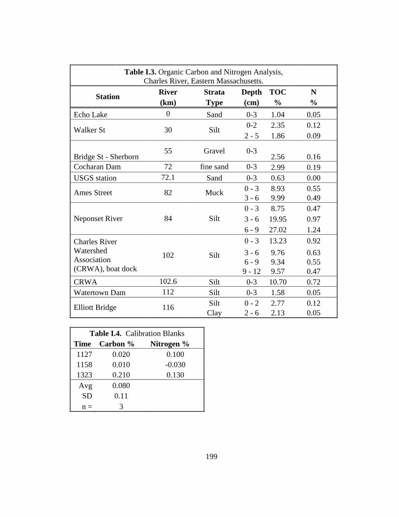
199

Table I.3. Organic Carbon and Nitrogen Analysis,

Charles River, Eastern Massachusetts.

Station River Strata Depth TOC N

(km) Type (cm) % %

Echo Lake 0 Sand 0-3 1.04 0.05

Walker St 30 Silt 0-2 2.35 0.12

2 - 5 1.86 0.09

Bridge St - Sherborn 55 Gravel 0-3

2.56 0.16

Cocharan Dam 72 fine sand 0-3 2.99 0.19

USGS station 72.1 Sand 0-3 0.63 0.00

Ames Street 82 Muck 0 - 3 8.93 0.55

3 - 6 9.99 0.49

Neponset River 84 Silt

0 - 3 8.75 0.47

3 - 6 19.95 0.97

6 - 9 27.02 1.24

Charles River

Watershed

Association

(CRWA), boat dock

102 Silt

0 - 3 13.23 0.92

3 - 6 9.76 0.63

6 - 9 9.34 0.55

9 - 12 9.57 0.47

CRWA 102.6 Silt 0-3 10.70 0.72

Watertown Dam 112 Silt 0-3 1.58 0.05

Elliott Bridge 116 Silt 0 - 2 2.77 0.12

Clay 2 - 6 2.13 0.05

Table I.4. Calibration Blanks

Time Carbon % Nitrogen %

1127 0.020 0.100

1158 0.010 -0.030

1323 0.210 0.130

Avg 0.080

SD 0.11

n = 3

200

Table I.5. Analytical Blanks

Table 1.6. Difference from

Standard Reference Material

Time Carbon % Nitrogen %

Time Carbon Nitrogen

1220 -0.460 -0.080

1153 0.9% 1.3%

1225 0.090 -0.230

1230 -0.2% -0.3%

1415 0.230 -0.390

1420 0.8% 0.9%

1518 0.320 -0.200

1523 -0.1% -0.9%

1626 0.000 0.000

1631 -0.3% -0.7%

1218 0.160 -0.600

1223 -0.1% 0.0%

1454 0.470 -0.520

1500 4.0% 2.6%

1119 0.590 -0.590

0 0.2% -0.5%

1221 0.030 -0.110

1226 0.4% -0.2%

1332 -0.67 -0.2

1645 0.1% 0.8%

1528 0.03 -0.55

1621 1.3% 0.9%

1640 0.030 0.470

1723 1.9% 1.6%

0 0.250 -0.310

1759 1.4% -0.2%

1718 0.550 -0.080

1445 0.4% -8.6%

1754 1.380 0.120

2047 -1.1% 0.6%

1440 -0.050 0.190

2208 -0.6% -1.0%

0 0.090 -0.590

38 -0.9% 1.7%

33 0.380 -0.750

135 0.0% 0.2%

130 0.140 -0.630

237 0.7% 1.1%

232 -0.040 -0.710

Avg 0.005

Avg 0.176 SD 0.41

SD 0.01

Table I.7. Comparison of Duplicates

%C %N %H % Diff OC

e17d 2.852 6.1 0.31 -6.87%

e17 2.561 6.55 0.44

e31d 3.38 8.01 0.39 9.73%

e31 3.283 7.3 0.42

e43d 3.035 13.06 0.73 -3.97%

e43 3.762 13.6 0.86

e55d 2.197 24.58 1.64 0.16%

e55 2.595 24.54 1.71

e66d 2.29 26.09 1.51 6.75%

e66 2.3358 24.44 1.54

201

APPENDIX II

METAL ANALYSIS

II.1. Inductively Coupled Plasma – Mass Spectrometer

Metals, with the exception of mercury, were analyzed on an Inductively Coupled

Plasma-Mass Spectrometer ICP-MS. For each run, the standard calibration curves were

checked to ensure that the standard recoveries were sufficient for both the initial and final

curves. The net intensity values were blank adjusted and then adjusted according to the

calibration curve that provided the best fit to standards, the QC check standards that were

placed at every tenth analysis, and the standard reference materials. Matrix effects were

checked via samples spiked with known concentrations of prepared aqueous standards.

Analytical accuracy was further ensured by comparison of digestion duplicates and

analytical replicates. The concentration of each metal is reported below.

202

Table II.1. Box Pond limits of detection, average recovery for the SRMs, and the

average of the analytical and digestion duplicates.

LOD1

Avg. BCSS-

1 SRM

Recovery

Avg.

PACS-1

SRM

Recovery

Average of

Analytical

Replicates

Average

Difference

of

Digestion

Duplicates

27

Al 0.12 mg/g 103.2% 100.2% 1.50% 6.68% 57

Fe 0.01 mg/g 111.3% 108.7% -4.07% 0.80% 55

Mn 11.10 ng/g 125.73% 102.08% 0.88% -6.24% 65

Cu 0.25 ng/g 106.51% 101.58% -1.02% -9.41% 64

Zn 0.86 ng/g 119.19% 95.44% -1.66% 2.95% 206

Pb 0.04 ng/g 115.73% 98.52% -2.05% 9.11% 75

As 0.27 ng/g 106.00% 87.20% -4.53% 1.24% 110

Cd 0.01 ng/g 104.59% 110.37% 11.36% -7.44% 120

Sn 0.9 ng/g 95.79% 109.92% 1.32% -3.73% 52

Cr 5.4 ng/g 113.21% 106.12% 0.40% -25.03% 59

Co 0.59 ng/g 105.08% 92.25% 0.42% 11.18% 109

Ag 0.002ng/g No SRM -0.94% -2.64%

88Sr 2.76 ng/g No SRM -2.36% 15.21%

45Sc 3.14 ng/g No SRM -3.06% -13.74%

1 Based on 0.2 g of sample material.

203

Table II.2. Box Pond sediments, the range of values, and a comparison to the SRM

certified values.

Units Max Min BCSS-1 PACS-1

27Al mg/mL 67.79 32.40 62.6 ± 2.17 64.7 ± 1.16

57Fe mg/mL 42.27 4.87 32.9 ± 0.98 48.8 ± 0.84

55Mn µg/mL 596.88 71.56 229 ± 15 470 ± 12

65Cu µg/mL 467.12 -2.08 18.5 ± 2.7 452 ± 16

64Zn µg/mL 682.69 13.01 119 ± 12 824 ± 22

206Pb µg/mL 270.20 8.15 22.7 ± 3.4 404 ± 20

75As µg/mL 39.97 -0.25 11.1 ± 1.4 211 ± 11

110Cd µg/mL 5.30 0.13 0.25 ± 0.04 2.38 ± 0.2

120Sn µg/mL 257.32 -0.21 1.85 ± 0.2 41.1 ± 3.1

52Cr µg/mL 246.65 4.31 123 ± 14 113 ± 8

59Co µg/mL 14.20 0.67 11.4 ± 2.1 17.5 ± 1.1

109Ag µg/mL 11.82 0.03

No SRM Available 88Sr µg/mL 163.83 51.78

45Sc µg/mL 12.22 2.37

204

Table II.3. Echo Lake limits of detection, average recovery for the SRMs, and the

average of the analytical and digestion duplicates.

LOD1

Avg.

BCSS-1

SRM

Recovery

Avg.

PACS-1

SRM

Recovery

Average

Difference

of

Analytical

Replicates

Average

Difference

of

Digestion

Duplicates

27Al 0.12 mg/g 97.50% 102.44% 0.82% 4.24%

57Fe 0.03 mg/g 101.39% 96.64% -1.62% -3.46%

55Mn 2.06 mg/g 110.70% 104.52% 1.69% 4.45%

63Cu 1.7 ug/g 110.50% 100.60% 5.20% 4.71%

64Zn 41 ug/g 109.87% 102.52% 0.00% 2.47%

208Pb 0.80 ug/g 113.03% 103.96% -0.61% 2.68%

75As 5.23 ug/g 105.99% 91.23% -3.38% 0.03%

114Cd 0.36 ug/g 97.20% 104.07% 2.02% -1.30%

120Sn 6.21 ug/g 61.30% 110.39% 1.32% -3.73%

52Cr 5.26 ug/g 93.52% 91.02% -2.48% 1.39%

59Co 0.28 ug/g 110.14% 112.32% -0.88% 1.52%

107Ag 0.04 ug/g No SRM 2.35% 6.01%

88Sr 1.13 ug/g No SRM -1.25% 1.75%

45Sc 1.76 ug/g No SRM 3.71% 2.37%

1 Based on 0.2 g of sample material.

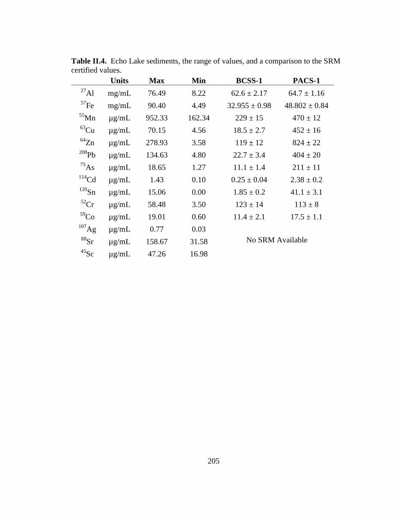
205

Table II.4. Echo Lake sediments, the range of values, and a comparison to the SRM

certified values.

Units Max Min BCSS-1 PACS-1

27Al mg/mL 76.49 8.22 62.6 ± 2.17 64.7 ± 1.16

57Fe mg/mL 90.40 4.49 32.955 ± 0.98 48.802 ± 0.84

55Mn µg/mL 952.33 162.34 229 ± 15 470 ± 12

63Cu µg/mL 70.15 4.56 18.5 ± 2.7 452 ± 16

64Zn µg/mL 278.93 3.58 119 ± 12 824 ± 22

208Pb µg/mL 134.63 4.80 22.7 ± 3.4 404 ± 20

75As µg/mL 18.65 1.27 11.1 ± 1.4 211 ± 11

114Cd µg/mL 1.43 0.10 0.25 ± 0.04 2.38 ± 0.2

120Sn µg/mL 15.06 0.00 1.85 ± 0.2 41.1 ± 3.1

52Cr µg/mL 58.48 3.50 123 ± 14 113 ± 8

59Co µg/mL 19.01 0.60 11.4 ± 2.1 17.5 ± 1.1

107Ag µg/mL 0.77 0.03

No SRM Available 88Sr µg/mL 158.67 31.58

45Sc µg/mL 47.26 16.98

206

Analytical results for the Echo Lake and Box Pond cores are shown below in

groups of figures. The Echo Lake results are followed by the Box Pond values. Within

Echo Lake and Box Pond the metals are grouped by crustal indicator metals, Al, Sr, Sc

and Co, by the redox indicators, Fe, Mn, Cr and Total Organic Carbon, by the

anthropogenic metals, Cu, Zn, Ag, and Sn, and by the toxic metals Hg, Pb, As, and Cd.

These are the values as detected by the ICP-MS except for Hg which was determined on

the CETAC instrument and TOC on the Perkin-Elmer CHN detector. The y-axis in each

case is the depth in cm of the core and the x-axis is the concentration. Each of these

metal results will be discussed in the relevant chapters as they bear on the findings.

In examining the metal concentrations, for the bulk of the research, the values will

be plotted against the year of deposition to derive a history of metal deposition in

sediment. Where appropriate the metal results will be processed to remove the crustal

contribution and derive a deposition rate, moles/m2/year that will be plotted against the

year of deposition.

The values that follow display the concentration against depth with the error bars.

This format will enable the reader to more easily determine concentration ranges and

trends. The actual data for each data set are contained in Excel sheets appended

separately.

207

Figure II.1. Echo Lake sediment core crustal metals.

-5

0

5

10

15

20

25

30

35

40

0 20 40 60 80

Dep

th (

cm)

Echo Lake

Aluminum (mg/g)

-5

0

5

10

15

20

25

30

35

40

0 40 80 120 160 200

Dep

th (

cm)

Echo Lake

Strontium (µg/g)

-5

0

5

10

15

20

25

30

35

40

0 5 10 15 20

Dep

th (

cm)

Echo Lake

Cobalt (µg/g)

-5

0

5

10

15

20

25

30

35

40

0 10 20 30 40 50 60

Dep

th (

cm)

Echo Lake

Scandium (µg/g)

208

Figure II.2. Echo Lake sediment core redox indicator metals and total organic carbon.

-5

0

5

10

15

20

25

30

35

40

0 20 40 60 80 100

Dep

th (

cm)

Echo Lake

Iron (mg/g)

-5

0

5

10

15

20

25

30

35

40

0 500 1000

Dep

th (

cm)

Echo Lake

Manganese (µg/g)

-5

0

5

10

15

20

25

30

35

40

0 20 40 60

Dep

th (

cm)

Echo Lake

Chromium (µg/g)

-5

0

5

10

15

20

25

30

35

40

0 10 20 30

Dep

th (

cm)

Echo Lake Total Organic

Carbon (moles/kg)

209

Figure II.3. Echo Lake sediment core anthropogenic metals.

-5

0

5

10

15

20

25

30

35

40

0 20 40 60 80

Dep

th (

cm)

Echo Lake

Copper (µg/g)

-5

0

5

10

15

20

25

30

35

40

0 100 200 300

Dep

th (

cm)

Echo Lake

Zinc (µg/g)

-5

0

5

10

15

20

25

30

35

40

0.00 0.50 1.00

Dep

th (

cm)

Echo Lake

Silver (µg/g)

-5

0

5

10

15

20

25

30

35

40

0 5 10 15 20

Dep

th (

cm)

Echo Lake

Tin (µg/g)

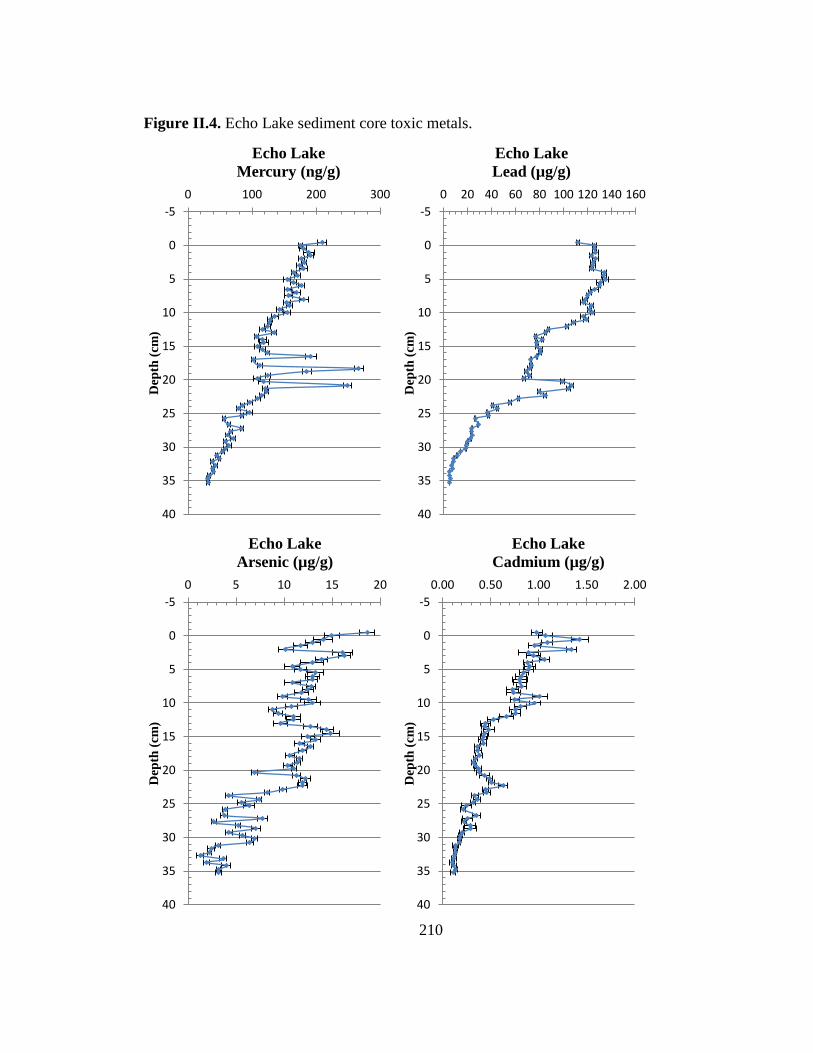
210

Figure II.4. Echo Lake sediment core toxic metals.

-5

0

5

10

15

20

25

30

35

40

0 100 200 300

Dep

th (

cm)

Echo Lake

Mercury (ng/g)

-5

0

5

10

15

20

25

30

35

40

0 20 40 60 80 100 120 140 160

Dep

th (

cm)

Echo Lake

Lead (µg/g)

-5

0

5

10

15

20

25

30

35

40

0 5 10 15 20

Dep

th (

cm)

Echo Lake

Arsenic (µg/g)

-5

0

5

10

15

20

25

30

35

40

0.00 0.50 1.00 1.50 2.00

Dep

th (

cm)

Echo Lake

Cadmium (µg/g)

211

Figure II.5. Box Pond sediment core crustal indicator metals.

0

5

10

15

20

25

30

0 20 40 60 80

Dep

th (

cm)

Box Pond

Aluminum (mg/g)

0

5

10

15

20

25

30

0 20 40 60 80 100 120 140 160 180

Dep

th (

cm)

Box Pond

Strontium (µg/g)

0

5

10

15

20

25

30

0 5 10 15 20

Dep

th (

cm)

Box Pond

Cobalt (µg/g)

0

5

10

15

20

25

30

0 5 10 15 20

Dep

th (

cm)

Box Pond

Scandium (µg/g)

212

Figure II.6. Box Pond sediment core redox indicator metals and total organic carbon.

0

5

10

15

20

25

30

0 20 40 60

Dep

th (

cm)

Box Pond

Iron (mg/g)

0

5

10

15

20

25

30

0 100 200 300 400 500 600

Dep

th (

cm)

Box Pond

Manganese (µg/g)

0

5

10

15

20

25

30

0 100 200 300

Dep

th (

cm)

Box Pond

Chromium (µg/g)

0

5

10

15

20

25

30

0 5 10 15

Dep

th (

cm)

Box Pond Total Organic

Carbon (moles/kg)

213

Figure II.7. Box Pond sediment core anthropogenic metals.

0

5

10

15

20

25

30

0 100 200 300 400 500

Dep

th (

cm)

Box Pond

Copper (µg/g)

0

5

10

15

20

25

30

0 100 200 300 400 500 600 700

Dep

th (

cm)

Box Pond

Zinc (µg/g)

0

5

10

15

20

25

30

0 5 10 15

Dep

th (

cm)

Box Pond

Silver (µg/g)

0

5

10

15

20

25

30

0 20 40 60

Dep

th (

cm)

Box Pond

Tin (µg/g)

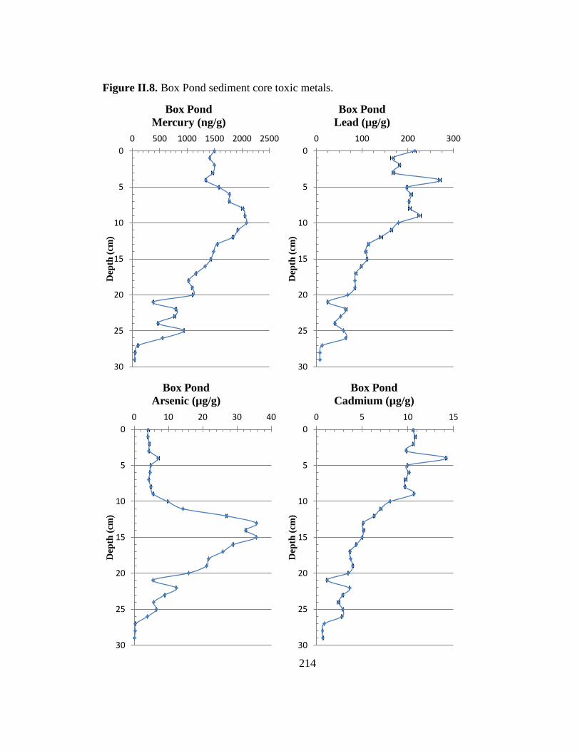
214

Figure II.8. Box Pond sediment core toxic metals.

0

5

10

15

20

25

30

0 500 1000 1500 2000 2500

Dep

th (

cm)

Box Pond

Mercury (ng/g)

0

5

10

15

20

25

30

0 100 200 300

Dep

th (

cm)

Box Pond

Lead (µg/g)

0

5

10

15

20

25

30

0 10 20 30 40

Dep

th (

cm)

Box Pond

Arsenic (µg/g)

0

5

10

15

20

25

30

0 5 10 15

Dep

th (

cm)

Box Pond

Cadmium (µg/g)

215

II.2. Mercury Analysis

The data for mercury is displayed graphically in Section II.1., above. The QA/QC

for mercury analysis is described below.

Table II.5. Mercury blank results.

Echo Lake

Mercury

Blank ng/g

B1 5.92

B2 7.17

B3 2.22

B4 0.48

B5 1.29

B6 1.99

B7 3.71

B8 0.98

LOD 8.91

LOQ 29.71 Based on 0.2 g sample

Table II.6. Mercury Standard Reference Materials for Echo Lake

Echo Lake Reference Standard

Corrected Average STDev % Agreement

Concentration Concentration Concentration with

Sample_ID (ng/g) (ng/g) (ng/g) Certified Value

STD1 PACS 3910.81

4140 330 90.59% STD2 PACS 4629.43

STD3 PACS 4024.34

STD4 PACS 3995.62

PACS-1 Certified Value 4570 ±160

Box Pond

Mercury

Blank ng/g

B1 2.28

B2 7.34

B3 2.64

B4 -2.63

B5 -1.02

B6 7.71

B7 2.55

B8 3.19

LOD 8.27

LOQ 27.57 Based on 0.2 g sample

216

Table II.7. Mercury Standard Reference Materials for Box Pond.

Box Pond Reference Standard

Corrected Average STDev % Agreement

Concentration Concentration Concentration with

Sample_ID (ng/g) (ng/g) (ng/g) Certified Value

Std2 Pacs1 4849.94

4724 257 103.36%

Std2 Pacs1-b 5011.62

Std2 Pacs1-b 4784.13

Std1(b) 4536.70

Std1(b) 4661.82

Std 2 Pacs1 4272.87

Std 2 Pacs1 4948.48

PACS-1 Certified Value 4570 ±160

Table II.8. Analytical Replicates for Mercury, Echo Lake and Box Pond.

Box Pond Analytical Replicates

Conc. %

(ng/g) Agreement

B59R 69.59 100.42%

B59R-b 69.31

B43 415.65 103.20%

B43-b 402.75

B27 1595.97 101.57%

B27-b 1571.23

B9 1366.42 99.42%

B9-b 1374.41

G7 52.94 84.10%

G7-b 62.95

G17 584.06 91.96%

G17-b 635.11

Std2

Pacs1-b 4716.07 96.77%

Std2

Pacs1-b 4873.28

Std1(b) 4536.70 97.32%

Std1(b) 4661.82

Std 2

Pacs1 4272.87 86.35%

Std 2

Pacs1 4948.48

Average 95.68%

Echo Lake Analytical Replicates

Conc. %

(ng/g) Agreement

E'2 208.46 100.30%

E'2(R) 207.84

E'10 182.20 103.82%

E'10(R) 175.48

E'19 181.27 101.47%

E'19(R) 178.65

E'27 122.99 99.76%

E'27(R) 123.28

E'36 190.83 100.06%

E'36(R) 190.72

E'43 115.71 96.88%

E'43(R) 119.44

E'52 96.04 101.70%

E'52(R) 94.43

E'59 69.98 98.81%

E'59(R) 70.82

E'67 42.12 96.46%

E'67(R) 43.66

E'72a 34.28 112.30%

E'72a(R) 30.53

Average 101.16%

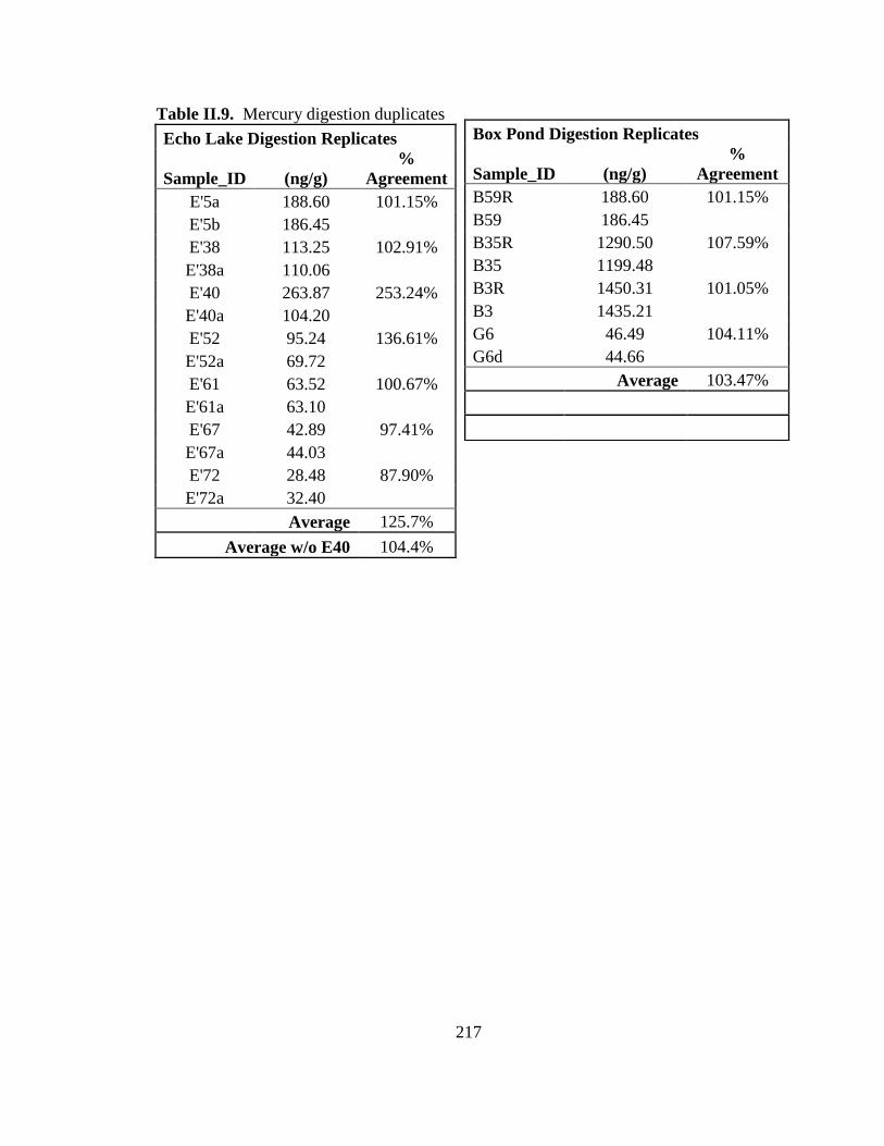
217

Table II.9. Mercury digestion duplicates

Echo Lake Digestion Replicates

Sample_ID (ng/g)

%

Agreement

E'5a 188.60 101.15%

E'5b 186.45

E'38 113.25 102.91%

E'38a 110.06

E'40 263.87 253.24%

E'40a 104.20

E'52 95.24 136.61%

E'52a 69.72

E'61 63.52 100.67%

E'61a 63.10

E'67 42.89 97.41%

E'67a 44.03

E'72 28.48 87.90%

E'72a 32.40

Average 125.7%

Average w/o E40 104.4%

Box Pond Digestion Replicates

Sample_ID (ng/g)

%

Agreement

B59R 188.60 101.15%

B59 186.45

B35R 1290.50 107.59%

B35 1199.48

B3R 1450.31 101.05%

B3 1435.21

G6 46.49 104.11%

G6d 44.66

Average 103.47%

218

II.3. Surface Sediment Samples

Thirteen surface sediment samples were examined in Chapter 5. The analysis of

the these samples, with respect to blanks, duplicates and methods were identical to those

outlined in the above sections regarding the TOC, ICP-MS and CVAA analyses for the

sediment cores. The location of the grab samples is shown in Table II.10.

Table II.10. Surface sediment sampling locations and the approximate distance from the

Charles River dam.

Sample Location Station

Town (km) Latitude Longitude

Echo Lake1 125 42º 11' 33.18" 71º 30' 29.97"

Echo Lake, Hopkinton 125.1 42º 11' 34.91" 71º 30' 29.38"

Box Pond2, Bellingham 111 42º 05' 41.35" 71º 29' 05.20"

Walker Street, Medway 95 42º 08' 24.01" 71º 23' 23.03"

Bridge Street, Sherborn 70 42º 13' 56.51" 71º 19' 49.51"

Cocharan Dam, Dover 53 42º 15' 30.17" 71º 15' 47.16"

USGS station, Dover 52.9 42º 15' 28.79" 71º 15' 46.24"

Ames Street, Dedham 43 42º 15' 09.21" 71º 10' 38.36"

Neponset River, Boston 41 42º 15' 15.87" 71º 10' 19.33"

CRWA Dock, Newton 23 42º 20' 41.11" 71º 15' 36.44"

CRWA Bank, Waltham 22.4 42º 20' 49.27" 71º 15' 34.53"

Watertown Dam, Watertown 13 42º 21' 54.57" 71º 11' 25.60"

Elliott Bridge, Cambridge 9 42º 21' 14.77" 71º 07' 57.43"

219

Table II.11. Community Data along the Charles River.

Population

Density

Residential

Land use

Commercial,

industrial &

transportation

Land use

(People/km2) (%) (%)

Hopkinton, Echo

Lake 185 24% 5%

Milford, MA 690 37% 11%

Bellingham 313 27% 7%

Franklin 423 33% 6%

Medway 411 40% 3%

Norfolk 262 30% 3%

Millis 248 23% 3%

Medfield 325 32% 2%

Dover 139 28% 0%

Sherborn 101 22% 0%

Natick 776 47% 10%

Needham 872 50% 8%

Dedham 847 39% 14%

Wellesley 978 60% 5%

Weston 256 44% 4%

Newton 1778 63% 9%

Watertown 3106 50% 22%

Cambridge 5435 37% 29%

Boston 4603 41% 30%

Charles River

Watershed 1286

220

APPENDIX III

GEOCHRONOLOGY

III.1. Introduction

Radioisotope geochronology using non-destructive gamma detection of 210

Pb, 214

Pb

and 137

Cs, was used to determine the absolute ages of each horizon of two sediment cores

(Appleby and Oldfield 1978; Schell and Barnes 1986). The method of collection and

preparation of the sediment cores are described in Chapter 2.

The natural radioisotope 210

Pb, an intermediate daughter product in the 238

U decay

chain, was used to determine the date of deposition for each of the 5 mm sediment layers.

The short-lived radioisotope 214

Pb was used to separate the in situ (supported) 210

Pb from

that deposited from the atmosphere (excess). Radioisotope dating with 210

Pb is generally

limited to 5 times the half-life, 22.3 years, which is approximately 110 years (Appleby

and Oldfield 1978). Gamma emissions from 210

Pb and 214

Pb were detected at 46 keV and

295 keV, respectively, in this research.

The man-made isotope 137

Cs is produced by nuclear fission and serves as an

excellent marker isotope in sediment, under optimal conditions this isotope shows the

onset of above ground nuclear testing circa 1954 and the crescendo of U.S.-Soviet above

ground atomic bomb testing in 1963. The gamma rays of 137

Cs were detected at energy

levels of 661 keV.

Once the gamma emissions have been measured it is necessary to apply efficiency

corrections to determine the true activity of each radioisotope. The necessary corrections

221

are for branching, detector efficiency, geometry and self-adsorption. Branching

efficiency is a measure of the number of decays that produce a gamma ray. Branching is

a literature value that has been determined through other works (Schell and Barnes 1986).

Detector efficiency is the percentage of gamma decays that pass through the detector that

are counted. Because no detector can intercept all gamma ray emissions, and the detector

used in this research was a planar detector, geometry corrections consider how many of

the gamma decays pass through the detector. Both detector efficiency and geometry

corrections were measured using Standard Reference Material 4350B, from the National

Bureau of Standards with a known activity and a reference date of September 9, 1981.

Pitchblende ore, Certified Reference Material CRM 101-A, was also used to determine

efficiencies and was used in the construction of a button standard to determine self-

adsorption in the sediment samples.

Self-absorption was measured by the use of a button source that was deployed on top

of the sample using the method of Cutshall (Cutshall et al. 1983). Self-adsorption was

determined for each sample by counting a sample to determine the activity in that sample

and then placing a button standard on top of the sample and repeating the count.

The button standard was a plastic vial with a volume of 2.4 cm3

and a wall thickness

of 1mm containing a source material of 0.8 cm thickness and approximately 1.8 cm

diameter. The button was weighed empty, packed only with a pitchblende ore, re-

weighed on a Sartorius scale (1/10,000th g precision) and sealed with tape. The ore used

inside the button consists of the CRM 101-A pitchblende ore - silica mixture from the

U.S. Department of Energy New Brunswick Laboratory. The amount of uranium is

certified as 1.007 0.013 wt.% ( = 0.05, df = 36).

222

For the construction of the button standard the New Brunswick Laboratory

Certificate of Analysis states that the Uranium content of the pitchblende ore - silica

mixture is 1.007 " 0.013 Wt.% (" = 0.05, df = 36). Assuming secular equilibrium, the

number of atoms of each species, and therefore the activities, of each of the parents and

daughters are related through their decay constants at any one instant based on

AparentNparent= AdaughterNdaughter. The amount of ore in the constructed button standard for

this work is 2.7427 g. Based on the weight of the ore/silica mixture there should be

0.02762 g of uranium in the button. This translates to 0.0001152 moles of 238

U using the

atomic weight of 238.029 g/mole. The number of atoms of 238

U in our button therefore is

6.938 x 1019

. Multiplying the decay constant of 238

U, (0.6931/(4.468 x 109 x 3.156 x

107sec/year)) the decay probability per second, by the number of atoms yields the number

of decays per second:

4.915x10-18

x 6.98805x1019

= 344.48 decays per second (dps)

Equation 1

For secular equilibrium this number, 344.48 decays per second, or Becquerels

(Bq), then cascades throughout the decay chain. The above calculation is for a button

standard that weighs 2.7427 g. To get the decay per gram, one simply divides the decays

per second by the grams in the button standard to arrive at the theoretical activity of

125.60 Bq/g. Figure III.1 depicts the measurement of a sample and measurement of the

self-adsorption.

223

Figure III.1. Photographs of a sample measured on the LEGe detector (left) and the

same sample with the button standard for determining self-adsorption (right).

For this work the following values were determined:

210Pb at energy 46keV the combined branching, geometry and detector efficiency

was determined to be 0.5114% and the value of self adsorption varied between the

samples, but averaged 1.1160 for the Box Pond samples and 1.1247 for the Echo

Lake samples.

214Pb at energy 295keV the combined efficiency was determined to be 0.06835%

and the value of self adsorption averaged 1.1076 for the Box Pond samples and

1.0087 for the Echo Lake samples.

137Cs at energy 661keV the combined efficiency, including that for self

adsorption, was determined using a 4350b standard and was determined to be

1.4%.

For each of the sediment cores, all error values were propagated from the original

data. All data were also decay corrected to represent the activity present in the

sample on the date of collection.

224

To determine the age dates of the various horizons in the sediment it is necessary

to apply a model of the presumed deposition method of the sediment. The primary

models used were the Constant Flux/Constant Sedimentation (CF/CS) model, the

Constant Rate of Supply (CRS) model, and the Constant Initial Concentration (CIC)

model. The use of these models is well described in the literature (Appleby and

Oldfield 1992). For both sediment cores all models were used and compared to

determine the sensitivity of the dating methods.

The models use the activity of the excess 210

Pb derived from the overall activity

subtracting the activity of 214

Pb, assuming secular equilibrium. The plots of the

resulting activities of excess 210

Pb and 137

Cs for the Box Pond and Echo Lake

sediment cores, and the associated 1-σ error, are shown in Figures III.2 and III.3,

respectively:

225

Figure III.2. Activity of excess 210

Pb data and 137

Cs in the Box Pond sediment core.

The data are plotted against depth from the surface water/sediment interface. To make

the data comparable, the 137

Cs activity was multiplied by 10.

Figure III.3. Activity of excess 210

Pb data and 137

Cs in the Echo Lake sediment core.

The data are plotted against depth from the surface water/sediment interface. To make

the data comparable, the 137

Cs activity was multiplied by 10.

0

5

10

15

20

25

30

0.0 0.1 0.2 0.3 0.4 0.5 0.6 0.7

Dep

th (

cm

) Activity (Bq/g)

xs Pb-210

Cs-137 (values x 10)

0

5

10

15

20

25

30

35

0.0 0.1 0.2 0.3 0.4 0.5 0.6 0.7

Dep

th (

cm

)

Activity (Bq/g)

xs 210Pb

137Cs (x 10)

226

III.2. Box Pond

The Box Pond profile in Figure III.2 displays the typical excess 210

Pb decline with

depth and 137

Cs peak at 1963. The three dating methods were in relatively good

agreement at the top and bottom of the core. However, in the middle portion of the core a

difference develops between the CF/CS method and the variable methods as shown in

Figure III.4. Despite concurrence between the two variable methods, an examination of

the data led to selection of the CF/CS method of dating as the more accurate by reason of

the 137

Cs peak aligning with the 1963 date whereas the variable methods have the 1963

peak in the 1980s.

227

Figure III.4. Comparison of the dating models for the Box Pond sediment core.

0

5

10

15

20

25

30

1750 1800 1850 1900 1950 2000

Dep

th (c

m)

Year

Comparison of Models - Box Pond

CFCS

CRS

CIC

In Figure III.4 a comparison of the results of running each of the models shows

better agreement of the CF/CS to the data. This model was applied to the sediments with

a sedimentation rate of 3 mm yr-1

. The red line in Figure III.4 represents the year 1963

and the arrows depict where in the sediment the CF/CS (upper) and CRS and CIC (both

lower) represent the data. The accepted geochronology for the Box Pond core is shown

below in Table III.1 the data and worksheets are in the attached Excel spreadsheets.

228

Table III.1. Stratigraphy and geochronology of Box Pond. Each depth interval has an

assigned year and associated error.

Box Pond Geochronology Accepted Date

Description of Depth, top prop. Error

Stratigraphy of of section 1-σ

Core (cm) Year value (yrs)

liquid black gel 0 2000 0.00

Floc 0.5 1998 0.13

1 1997 0.11

1.5 1995 0.09

2 1993 0.11

2.5 1992 0.14

3 1990 0.12

more cohesive 3.5 1988

black 4 1987 0.17

4.5 1985

5 1984 0.17

5.5 1982

6 1980 0.10

lots of leaves 6.5 1979

7 1977 0.14

7.5 1975

8 1974 0.15

8.5 1972

9 1970 0.15

9.5 1969

10 1967 0.15

10.5 1965 0.16

11 1964 0.11

11.5 1962 0.12

12 1960 0.15

big rock 12.5 1959

13 1957 0.21

13.5 1956

14 1954 0.17

14.5 1952

black, clay-like 15 1951 0.19

15.5 1949

16 1947 0.11

16.5 1946

17 1944 0.19

17.5 1942

18 1941 0.18

18.5 1939

19 1937 0.19

19.5 1936

20 1934 0.15

20.5 1932

229

Box Pond Geochronology Accepted Date

Description of Depth, top prop. Error

Stratigraphy of of section 1-σ

Core (cm) Year value (yrs)

21 1931 0.11

21.5 1929

22 1928 0.16

22.5 1926

23 1924 0.15

23.5 1923

24 1921 0.12

24.5 1919

25 1918

25.5 1916

Coarse sand 26 1914 0.14

26.5 1913

27 1911

27.5 1909

28 1908

28.5 1906

29 1905 0.20

29.5 1903

The bold dates with the 1-sigma values are derived from the CF:CS method of dating. The regular type dates without error are estimated from the surrounding values and used for plotting purposes.

III.3. Echo Lake

The Echo Lake sediment core activity profile for excess 210

Pb shown in Figure III-3

shows two anomalous features. First, the 1963 bomb peak of 137

Cs is absent and, second,

applying the CF/CS method using excess 210

Pb in the 11.5 to 13.5 cm segment of the

profile shows an unrealistic slow rate of sedimentation, approximately 0.06 cm yr-1

of

sediment accumulation. By contrast the lower and upper sediments that bound this

region have rates of 0.3 and 0.4 cm yr-1

, respectively.

Examining the inventories of both the Echo Lake and Box Pond cores proved

diagnostic. The Box Pond core has an excess 210

Pb inventory of approximately 4000 Bq

230

m-2

, 20% lower than the average for a similar impoundment in North Andover, 5200

Bq∙m-2

(Wallace et al. 2004) and lower than the regional average of 5654 ± 3907 Bq∙m-2

but within the range of error (Appleby and Oldfield 1992). The 137

Cs inventory in Box

Pond is approximately 700 Bq∙m-2

which yields a ratio of 5.6/1, 210

Pb/ 137

Cs, respectively.

By contrast, Echo Lake has a 210

Pb inventory of approximately 8200 Bq∙m-2

and a

137Cs inventory of approximately 1100 Bq∙m

-2 a ratio of 7.2/1,

210Pb/

137Cs, respectively.

The excess inventory of 210

Pb over that of the regional value and that found in a North

Andover impoundment indicates that the Echo Lake location is likely a point sediment

focusing. Yet, the apparent deficiency of 137

Cs relative to the 210

Pb indicates that some

material is missing from the Echo Lake core.

The morphology of Box Pond and Echo Lake are very different. Box Pond is

narrow and shallow, while Echo Lake is wide and comparatively deep. The sediment

core collection point for Box Pond, although in the deepest point near the dam, is less

than 2 m deep and therefore subject to some of the effects of erosion at high energy flows

in the river. High flows were witnessed during the sediment core collection in January

2000. Therefore, some loss of material is expected on a seasonal or episodic basis. The

Echo Lake sediment core location has few erosive forces and during most times of the

year is under more than 8 m of water. It is more likely that the location of the sediment

core collection in Echo Lake is a site of sediment focusing (Davis and Ford (Jesse) 1982).

Initially, the CF/CS model was applied to segments of the data. Those calculations are in

the Excel spreadsheets, and the results are shown in Figure III.5, below:

231

Figure III.5: Natural log of activity of excess 210

Pb in the Echo Lake sediment core.

The sedimentation rates for different segments of the profile are calculated. The

stratigraphy of the Echo Lake sediment core is also described on the figure. Red arrows

point to 3 of the 5 segments of differing deposition rates determined for the excess 210

Pb

profile.

The key issue in Figure III.5 is that despite the consistent stratigraphy in the

sediments with roots and fibers, there appear to be three separate deposition rates in the

upper 20 cm of the sediment core. The interval between 11.5 and 13 cm, Zone 2, is not

visually different from the interval above or below and it appears very coherent, despite it

0

5

10

15

20

25

30

0.00 0.50 1.00 1.50 2.00 2.50 3.00 3.50 4.00

Dep

th (

cm

)

LN Activity xs 210Pb (Bq/s)

Echo Lake Sediment Core Stratigraphy and

Gray, cake-like.

Sediment with

many roots and

fibers.

Peat

Zone 2 Sed rate 0.06 cm/year

Gray, cake-like.

Sediment with

many roots and

fibers.

Peat



Terrestrial, leaves and grass.


232

having a sedimentation rate that is five times lower than that above and below it. Taking

this profile and dating the segments using the CF/CS model finds that the top of Zone 2

has a date of 1969 while 2 cm below it has a date of 1927, a span of nearly 40 years. The

fraction of dry weight points to the significance of the 11.5 to 13 cm interval as shown on

Figure III.6.

Figure III.6. Fraction dry weight of the Echo Lake sediments. This is a dimensionless

number plotted against the depth and is calculated by dividing the dry weight for each 5

mm section by the weight of wet sediment.

Typical profiles of the fraction of dry weight show an increase with depth, which is

what occurs in the upper 13 cm. At 13.5 cm to 19.8 cm, the density becomes less with

depth, counter to the typical trend. There appeared to be no visual difference in the

0

5

10

15

20

25

30

35

40

0.00 0.10 0.20 0.30 0.40

Dep

th (

cm

)

Dry Sediment/Wet Sediment & Water (wt/wt)

Fraction of Dry Weight

233

sediments from 7.5 to 19.8 cm. Below 19.8 cm, peat dominates the stratigraphy and

maintains a consistent composition and density.

The slow rate of deposition and the apparent change in trend of fraction of dry

weight in the interval between 11.5 and 13.5 cm point to a change in deposition when this

interval was deposited. There are several possibilities for the deposition rate for this

interval which may impact the radiometric dating and the overall observations in the

sediment core regarding metal concentrations:

1. Loss of material that occurred either during coring or in 1968.

a. The core was collected by a diver using a wide coring device. However,

this seems unlikely.

b. In 1968, eastern Massachusetts had extensive floods that impacted the

Charles River and could have created an erosion event. However, an

erosion event is unlikely as the watershed is quite small and the standing

pool above the coring site in excess of 6 m.

c. Also in 1968, the Milford water company installed a pipe in the bottom of

the dam to pipe water to its treatment plant. The installation of that pipe,

by a diver, may have impacted the sediment core site by removing

material.

d. Bioturbation, an organism could have removed some portion of the

sediment for a redd (fish) or for hibernation (turtle).

e. It is noted that this section has many roots indicating that plants grew

profusely in this area. The plants could have been uprooted by some

event, such as the preceding, and thus removed the sediment.

234

2. A plant or other material on the lake bottom may have created a sediment shade in

the area of the core.

The low sedimentation rate, coupled with the apparent deficiency of 137

Cs in the

core, indicated that some amount of material was removed from the sediment record in

this location. This area is termed the “Disturbed interval” throughout this research.

One counter-argument to the removal of material might be that the Disturbed

interval between 11.5 and 13 cm appears to have a trend in the activity of excess 210

Pb;

however, that may be explained by the nature of the material. The hypothetical erosion

event would suspend the sediment wherein some is removed, while some portion settles

out of the turbidity cloud created after removal. The heavier particles, which would be

less particle-reactive and therefore would contain less 210

Pb would settle first, and the

finer material which would be more particle reactive would settle last.

Regardless of the mechanism, some portion of the sediment record from 11.5 to 13.5

cm is missing. To determine how much material was removed from the Echo Lake

sediment record it was assumed that the missing material would have a logarithmic

function similar to the sediments above and below the Disturbed interval (Appleby and

Oldfield 1992). To determine the amount of missing material, the excess 210

Pb activity

profile was graphically split into three segments: upper (0 to 11 cm), Disturbed interval

(11.5 to 13 cm) and lower (13.5 to 34 cm). The upper segment remained stationary while

the lower segment was moved downward and a logarithmic regression applied to the new

configuration. The best-fit logarithmic regression was with 13 cm of separation between

upper and lower segments as shown in Figure III.7:

235

Figure III.7. Analysis of the Disturbed interval: a) The activity of excess 210

Pb in the

Echo Lake sediment core is shown with the problem interval, 11.5 to 13.5 cm

highlighted. b) Separates the data into three segments: upper activity, Disturbed interval,

and lower activity. The plot of the excess 210

Pb for the upper 11.5 cm remains as in (a)

but moves the data below 13.5 cm downward until the best fit line was determined with a

R2

value of 0.96.

The Disturbed interval shown in Figure III.7b was stretched over the amount of

material removed from the sediment record in this area. This work is shown in greater

detail in the Excel sheet Geochron Echo Lake.xlsx. The conclusion of the analysis was

that approximately 13 cm was removed from the sediment record between 11.5 and 13.5

cm.

The missing mass and activity, based on the sediment horizons above and below the

Disturbed interval, was added back to the sediment core. Adding the missing 210

Pb

y = -7.07n(x) + 26.07 R² = 0.91

0

5

10

15

20

25

30

35

40

0 10 20 30 40

De

pth

(c

m)

Activity (dpm/g)

a. Activity 210Pb

Disturbed Interval

y = -9.82ln(x) + 34.22 R² = 0.96

0

5

10

15

20

25

30

35

40

0 10 20 30 40

De

pth

(c

m)

Activity (dpm/g)

b. Disturbed Interval inserted

Upper Activity

Lower Activity

Missing Interval

Disturbed Interval

236

inventory to the overall inventory yielded a total inventory of approximately 11,000 Bq

m-2

. If 11,000 Bq m-2

were the total sediment core inventory, it would be approximately

twice that of the expected inventory for this region indicating that the sediment focusing

factor was approximately twice the typical rate (Davis and Ford (Jesse) 1982; Appleby

and Oldfield 1992). The Box Pond ratio of the inventories of excess 210

Pb:137

Cs was

5.71:1. Using the Box Pond ratio, the expected inventory of Echo Lake 137

Cs based on

the activity of 210

Pb, should be approximately 1900 Bq m-2

. The actual inventory of Echo

Lake 137

Cs was 1100 Bq m-2

, a deficit of 800 Bq m-2

of what would be expected. The

inventory of Box Pond 137

Cs over the period of the Disturbed interval, 1920 to 1969, is

436 Bq m-2

. If sediment focusing at Echo Lake is considered to be twice typical

locations, the expected inventory of 137

Cs based on the ratio found at Box Pond, is 872

Bq m-2

similar to the calculated deficit of 800 Bq m-2

.

The CF/CS model was used to determine the dates of the Echo Lake sediment core

in the upper segment. The dates of deposition for the metal concentrations in the

Disturbed interval are assigned and if erosion was the source of the unconformity, would

not be accurate, but if it were the product of shading may have some relevance to the

dates shown. The lower segment was dated by inserting the missing inventory, and then

using the CRS model to determine dates. All models were run and the CRS was chosen

as it demonstrated the best agreement with stratigraphic breaks in the sediment core. At

19.3 cm the sediment transitioned from terrestrial debris to lake sediment. The 19.3 cm

layer was believed to be when the dam filled in 1882. Although the 1850 date is beyond

the accepted accuracy of the 210

Pb method, a local resident said that two sisters had

237

maintained Echo Lake as a hayfield from the 1850’s (Bowker 2005). Excel sheets

provide an analysis of the data and the methods used.

The application of the 210

Pb geochronology dating methodology is typically for only 5

half-lives, 110 years, or approximately 1899 in this instance (Appleby and Oldfield

1978). The dating model’s correspondence of 1882 with the known date of the lake’s

creation provided confidence in the model’s accuracy. When the strata transitioned to

peat, the model’s results were extended downward based on the calculated accumulation

rate of 8 yr cm-1

, which is comparable to other values in the literature. A similar peat bog

in Switzerland had accumulation rates of approximately 10 yr cm-1

calculated using 14

C

methods (Shotyk et al. 2000).

The final, accepted dates of the sediment core are shown in Table III.2. Error values

are only supplied for the upper 11.5 cm because the uncertainty below that horizon is

unknown.

238

Table III.2. Stratigraphy and geochronology of Echo Lake. Each depth interval has an

assigned year and associated error. The dates 1959 to 1929 represent the result of a

period of missing deposition and are speculative. No error was calculated for the

intervals below the Disturbed interval. Summaries of observations regarding the

sediment core are shown inside the stratigraphy. Cored Error

Core Description Depth Accepted Value

(cm) Year Years

Black soup. 0 1998 0.07

0.5 1997 0.11

1 1997 0.13

1.5 1997 0.16

Black, but coherent. 2 1996 0.20

2.5 1995 0.25

A little clay, black and 3 1994 0.33

very coherent. 3.5 1993 0.40

4 1991 0.50

4.5 1990 0.58

Less coherent than 5 1989 0.64

above. 5.5 1988 0.70

6 1987 0.78

Clay, cake-like. 6.5 1986 0.86

7 1984 1.00

Roots, fibers and 7.5 1983 1.06

vegetative matter. 8 1981 1.15

8.5 1980 1.25

9 1978 1.36

9.5 1977 1.44

10 1975 1.57

10.5 1972 1.73

11 1971 1.82

11.5 1969 1.95

Same as above, but 12 1959

more coherent 12.5 1949

and very fibrous. 13 1939

13.5 1929

14 1919

14.5 1915

Gray spots of clay 15 1912

present. 15.5 1908

16 1905

16.5 1903

17 1899

Fibrous and black. 17.8 1892

18.3 1890

18.8 1887

19.3 1882

Cut grass stems. 19.8 1879

20.3 1877

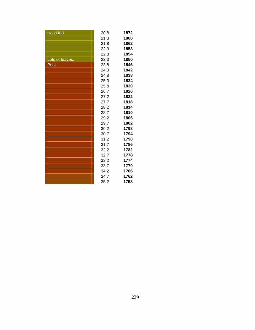
239

twigs too. 20.8 1872

21.3 1868

21.8 1862

22.3 1858

22.8 1854

Lots of leaves. 23.3 1850

Peat. 23.8 1846

24.3 1842

24.8 1838

25.3 1834

25.8 1830

26.7 1826

27.2 1822

27.7 1818

28.2 1814

28.7 1810

29.2 1806

29.7 1802

30.2 1798

30.7 1794

31.2 1790

31.7 1786

32.2 1782

32.7 1778

33.2 1774

33.7 1770

34.2 1766

34.7 1762

35.2 1758

240

REFERENCES

Appleby, P. G. and F. Oldfield (1978). "The calculation of Lead-210 dates assuming a

constant rate of supply of unsupported 210

Pb to the sediment." Catena 5: 1-8.

Appleby, P. G. and F. Oldfield (1992). Chapter 21 Application of Lead-210 to

Sedimentation Studies. Uranium-Series Disequilibrium: Applications to Earth,

Marine and Environmental Sciences. M. Ivanovich and R. S. Harmon. Oxford,

Clarendon Press, p. 910.

Aqua Doc Lake & Pond Management. (2009). Retrieved April 13, 2011, from

http://www.aquadocinc.com/Algaecides/Copper-Sulfate-(Granular)-15-lbs..html.

Barron, R. (1976). Natural Valley Storage: A partnership with nature. N. E. D.

Department of the Army, Corps of Engineers. Waltham, Massachusetts,

Department of the Army. DOD-314.

Benson, B. (2011). Milford, Franklin, Bellingham told to target phosphorous at the

source to protect Charles River. Milford Daily News. Milford, MA.

Berner, R. A. (1980). Early Diagenesis, A Theoretical Approach. Princeton, N.J.,

Princeton University Press, p. 256.

Boudreau, B. P. and B. B. Jorgensen, Eds. (2001). The Benthic Boundary Layer. New

York, Oxford University Press, p. 440.

Boutiette, L. N. J. and C. Duerring (1993). Massachusetts NonPoint Source Management

Manual. Boston, Massachusetts Department of Environmental Protection, Office

of Watershed Management.

Bowker, R. (2005). Personal interview. Hopkinton.

Brandenberger, J., P. Louchouran, et al. (2004). "Geochemical and hydrodynamic

controls on arsenic and trace metal cycling in a seasonally stratified US sub-

tropical reservoir." Applied Geochemistry 19: 1601 - 1623.

Breault, R. F., K. R. Reisig, et al. (2000). Distribution and Potential for Adverse

Biological Effects of Inorganic Elements and Organic Compounds in Bottom

Sediment, Lower Charles River, Massachusetts. Northboro, Massachusetts,

National Water-Quality Assessment Program, U.S. Department of the Interior,

U.S. Geological Survey.

http://www.aquadocinc.com/Algaecides/Copper-Sulfate-(Granular)-15-lbs..html

241

Brezonik, P. L., S. O. King, et al. (1991). The Influence of Water Chemistry on Trace

Metal Bioavailability and Toxicity to Aquatic Organisms. Metal Ecotoxicology:

Concepts & Applications. D. C. Adriano. Chelsea, Michigan, Lewis Publishers: 1

- 31.

Brimblecombe, P. and G. A. Dawson (1984). "Wet removal of highly soluble gases."

Journal of Atmospheric Chemistry 2: 95 - 107.

Brownlow, A. H. (1979). Geochemistry. Englewood Cliffs, N.J., Prentice-Hall, Inc, p.

580.

Chalmers, A. T., P. C. Van Metre, et al. (2007). "The chemical response of particle-

associated contaminants in aquatic sediments to urbanization in New England,

U.S.A." Journal of Contaminant Hydrology 91: 4 - 25.

Chapelle, F. H. (1993). Ground-Water Microbiology and Geochemistry. New York,

Wiley, p. 424.

Chapra, S. C. (1997). Surface Water Quality Modeling. Boston, McGraw-Hill, p.844.

Charles River Watershed Association (2000). Water Resources Conditions Update:

Upper Charles River Watershed. Auburndale, Massachusetts, Charles River

Watershed Association.

Charles River Watershed Association. (2005). "Water Resources and the Charles River:

A Fact Sheet." Retrieved January 26, 2005, 2005, from

http://www.crwa.org/index.html/wavestop.html.

Chi, K. H., S. Luo, et al. (2009). "Historical trends of dioxin-like compounds and heavy

metals in sediments buried in a reservoir in central Taiwan." Chemosphere 76: 7.

Chillrud, S. N., R. F. Bopp, et al. (1999). "Twentieth Century Atmospheric Metal Fluxes

into Central Park Lake, New York City." 33(5): 657-661.

Clements, W. H. (1991). Community Responses of Stream Organisms to Heavy Metals:

A Review of Observational and Experimental Approaches. Metal Ecotoxicology:

Concepts & Applications. D. C. Adriano. Chelsea, Michigan, Lewis Publishers:

363 - 391.

Coles, J. F., T. F. Cuffney, et al. (2004). The Effects of Urbanization on the Biological,

Physical, and Chemical Characteristics of Coastal New England Streams. Reston,

Virginia, National Water-Quality Assessment Program, U.S. Department of the

Interior, U.S. Geological Survey.

http://www.crwa.org/index.html/wavestop.html

242

Coles, J. F., T. F. Cuffney, et al. (2010). "Judging a Brook by its Cover: The

Relationship Between Ecological Condition of a Stream and Urban Land Cover in

New England." Northeastern Naturalist 17((1)): 29-48.

Commonwealth of Massachusetts (1953). Chapter 67 of the Resolves of 1953.

Commonwealth of Massachusetts (2009). Wetlands Protection. Massachusetts

Department of Environmental Protection. 310 Code of Massachusetts Regulations

10.00.

Commonwealth of Massachusetts (2010). Authorization to Discharge Under the National

Pollutant Discharge Elimination System. Massachusetts DEP: 38.

Commonwealth of Massachusetts. (2012). "Community Data." Retrieved March 13,

2012, 2012, from http://www.mass.gov/dep/service/my_comm/medway.htm.

Cooper, D. C., A. L. Neal, et al. (2005). "Effects of sediment iron mineral composition on

microbially mediated changes in divalent metal speciation: Importance of

ferrihydrite." Geochimica et Cosmochimica Acta 69(7): 1739 - 1754.

Cronon, W. (1983). Changes in the Land: Indians, Colonists, and the Ecology of New

England. New York, Hill and Wang, p. 242.

Cutshall, N. H., I. L. Larsen, et al. (1983). "Direct Analysis of 210Pb in sediment

samples: Self-adsorption corrections." Nucl. Instrum. Meth. 206: 309.

Davis, A. P., M. Shokouhian, et al. (2001). "Loading estimates of lead, copper, cadmium

and zinc in urban runoff from specific sources." Chemosphere 44: 997 - 1009.

Davis, M. B. and M. S. Ford (Jesse) (1982). "Sediment focusing in Mirror Lake, New

Hampshire." Limnology and Oceanography 27(1): 13.

Dichter, A. (2005). U.S. Environmental Protection Agency, Geographic Information

Section. Boston.

DiToro, D. M. (2001). Sediment Flux Modeling. New York, John Wiley & Sons, Inc, p.

448.

Doyle, M. W., E. H. Stanley, et al. (2003). "Dam Removal in the United States:

Emerging Needs for Science and Policy." American Geophysical Union, EOS

Transactions 84(4).

Drever, J. I. (1997). The Geochemistry of Natural Waters. Upper Saddle River, New

Jersey, Prentice Hall, p. 436.

http://www.mass.gov/dep/service/my_comm/medway.htm

243

Dunne, T. and L. B. Leopold (1978). Water in Environmental Planning. San Francisco,

W.H. Freeman and Co, p. 818.

Feng, H., X. Han, et al. (2004). "A preliminary study of heavy metal contamination in

Yangtze River intertidal zone due to urbanization." Marine Pollution Bulletin 49:

910 - 915.

Filgueiras, A. V., I. Lavilla, et al. (2004). "Evaluation of distribution, mobility and

binding behaviour of heavy metals in surficial sediments of Louro River (Galicia,

Spain) using chemometric analysis: a case study." Science of the Total

Environment 330: 115 - 129.

Flanagan, S. M., M. G. Nielsen, et al. (1999). Water Quality Assessment of the New

England Coastal Basins in Maine, New Hampshire, Massachusetts, and Rhode

Island: Environmental Settings and Implications for Water Quality and Aquatic

Biota. Pembroke, NH, U.S. Department of the Interior, U.S. Geological Survey.

Galloway, J. N., J. D. Thornton, et al. (1982). "Trace Metals in Atmospheric Deposition:

A Review and Assessment." Atmospheric Environment 16(7): 1677 - 1700.

Golomb, D., D. Ryan, et al. (1997). "Atmospheric Depostion of Toxics onto

Massachusetts Bay - 1. Metals." Atmospheric Environment 31(9): 1349 - 1359.

Goonetilleke, A., E. Thomas, et al. (2005). "Understanding the role of land use in urban

stormwater quality management." Journal of Environmental Management 74: 31 -

42.

Goyette, A. V. P. D. (1982). Milford Massachusetts Business Opportunity Book,

Department of Geography, Framingham State College.

Haglund, K. (2003). Inventing the Charles River. Cambridge, MA, The MIT Press, p.

512.

Hawley, G. G. (1977). The Condensed Chemical Dictionary. New York, Van Nostrand

Reinhold Company, p. 957.

He, F., W. Zheng, et al. (2012). "Mercury photolytic transformation affected by low-

molecular-weight natural organics in water." Science of the Total Environment.

Hedges, J. I. and J. H. Stern (1984). "Carbon and nitrogen determinations of carbonate-

containing solids." Limnology and Oceanography 29: 657-663.

Hildemann, L. M., G. R. Markowski, et al. (1991). "Chemical composition of emissions

from urban sources of fine organic aerosol." Environ. Sci. Technol.(25): 744 -

759.

244

Hill, R. (1975). Charles River Cleanup clogged by complexities. Globe. Boston.

Hill, R. (1975). Charles River cleanup costly. Globe. Boston.

Hopke, P. K., R. E. Lamb, et al. (1980). "Multielement characterization of urban roadway

dust." Environ. Sci. and Technol. 14: 164 - 172.

Hopkinton Planning Department (2004). Hopkinton, MA.

Ingersoll, C. G., P. S. Haverland, et al. (1996). "Calculation and Evaluation of Sediment

Effect Concentrations for the Amphipod Hyalella azteca and the Midge

Chironomus riparius." Journal of Great Lakes Research 22(3): 602-623.

Kalff, J. (2002). Limnology, Inland Water Ecosystems. Upper Saddle River, New Jersey,

Prentice Hall, p. 592.

Kamman, N. C. and D. R. Engstrom (2002). "Historical and present fluxes of mercury to

Vermont and New Hampshire lakes inferred from 210

Pb dated sediment cores."

Atmospheric Environment 36: 1599-1609.

Karouna-Renier, N. K. and D. W. Sparling (2001). "Relationships between ambient

geochemistry, watershed land-use and trace metal concentrations in aquatic

invertebrates living in stormwater treatment ponds." Environmental Pollution Vol.

112: pp. 183 - 192.

Kolak, J. J., D. T. Long, et al. (1998). "Anthropogenic inventories and historical and

present accumulation rates of copper in Great Lakes sediments." Applied

Geochemistry 13: 16.

Kristensen, E. and F. O. Anderson (1987). "Determination of organic carbon in marine

sediments: a comparison of two CHN-analyzer methods." Journal of

Experimental Marine Biology and Ecology 109(1): 15-23.

Kylander, M. E., D. J. Weiss, et al. (2009). "Two high resolution terrestrial records of

atmospheric Pb deposition from New Brunswick, Canada, and Loch Laxford,

Scotland." Science of the Total Environment(407): 1644-1657.

Lennherr, I. and V. L. St. Louis (2009). "Importance of Ultraviolet Radiation in the

Photodemethylation of Methylmercury in Freshwater Ecosystems."

Environmental Science and Technology(43): 5692-5698.

Linsley, R. K., M. A.Kohler, et al. (1975). Hydrology for Engineers. New York, McGraw

Hill, p. 512.

245

Lovley, D. R. (1991). "Dissimilatory Fe(III) and Mn (IV) Reduction." Microbiological

Reviews 55(2).

Luoma, S. N. (1989). "Can we determine the biological availability of sediment-bound

trace elements?" Hydrobiologia(176/177): 379 - 396.

Luoma, S. N. and J. L. Carter (1991). Effects of Trace Metals on Aquatic Benthos. Metal

Ecotoxicology: Concepts & Applications. D. C. Adriano. Chelsea, Michigan,

Lewis Publishers: 261 - 301.

Macbeth, D. (1994). Munsell Soil Color Charts. New Windsor, NY.

MacKenzie, A. B., E. M. Logan, et al. (1998). "A historical record of atmospheric

depositional fluxes of contaminants in west-central Scotland derived from an

ombrotrophic peat core." The Science of the Total Environment(222): 157 - 166.

Mahler, B. J., P. C. Van Metre, et al. (2006). "Trends in metals in urban and reference

lake sediments across the United States, 1970 to 2001." Environmental

Toxicology and Chemistry 25(7): 1698 - 1709.

Mantoura, R. F. C., A. Dickson, et al. (1978). "The Complexation of Metals with Humic

Materials in Natural Waters." Estuarine and Coastal Marine Science 6: 387 - 408.

Massachusetts Department of Environmental Protection. (2011). "Municipal Waste

Combustors: Wheelabrator Millbury Technical Profile " Retrieved December 17,

2011, from http://www.mass.gov/dep/recycle/solid/wheelmpr.htm.

Massachusetts Water Resources Authority. (2005). "Water Supply and Demand."

Retrieved June 24, 2005, 2005, from

http://www.mwra.state.ma.us/04water/html/wsupdate.htm.

McAdow, R. (1992). The Charles River, Exploring Nature and History on Foot and by

Canoe. Marlborough, Massachusetts, Bliss Publishing Co., Inc.

Meylan, S., R. Behra, et al. (2003). "Accumulation of Copper and Zinc in Periphyton in

Response to Dynamic Variations of Metal Speciation in Freshwater." Environ.

Sci. Technol. 37: 5204 - 5212.

Milford Historical Commission (1980). History of Milford, Massachusetts, 1780 - 1980.

Milford.

Milford Historical Commission. (2004). "Milford History." Retrieved February 14,

2004, 2004, from http://milford.ma.us/pages/boards-committees/historical-

commission/milford-history.php.

http://www.mass.gov/dep/recycle/solid/wheelmpr.htm

http://www.mwra.state.ma.us/04water/html/wsupdate.htm

http://milford.ma.us/pages/boards-committees/historical-commission/milford-history.php

http://milford.ma.us/pages/boards-committees/historical-commission/milford-history.php

246

Morford, J. L. and S. Emerson (1999). "The geochemistry of redox sensitive trace metals

in sediments." Geochimica et Cosmochimica Acta 63(11/12): 1735 - 1750.

National Oceanic and Atmospheric Administration (1999). Sediment Quality Guidelines

developed for the National Status and Trends Program. National Oceanic and

Atmospheric Administration.

Neihof, R. and G. Loeb (1974). "Dissolved Organic Matter in Seawater and the Electric

Charge of Immersed Surfaces." Journal of Marine Research 32(1): 5 - 12.

Ohio History Central. (2005). "Cuyahoga River Fire", from

http://www.ohiohistorycentral.org/entry.php?rec=1642.

Olsen, C. R. (1979). Radionuclides, sedimentation and the accumulation of pollutants in

the Hudson River Estuary, Ph.D. Thesis, Columbia University: 343.

Olsen, C. R., N. H. Cutshall, et al. (1982). "Pollutant-Particle Associations and Dynamics

in Coastal Marine Environments: A Review." Marine Chemistry 11: 501 - 533.

Outridge, P. M., N. Rausch, et al. (2010). "Comparison of mercury and zinc profiles in

peat and lake sediment archives with historical changes in emissions from the Flin

Flon metal smelter, Manitoba, Canada." Science of the Total Environment.

Papuga, H. (2004). Manager, Milford Water Company.

Partridge, G. F. (1919). History of the Town of Bellingham, Massachusetts 1719 - 1919,

Town of Bellingham.

Pauleit, S., R. Ennos, et al. (2005). "Modeling the environmental impacts of urban land

use and land cover change - a study in Merseyside, UK." Landscape and Urban

Planning 71: 295 - 310.

Peeters, E. T. H. M., J. J. P. Gardeniers, et al. (2000). "Contribution of Trace Metals in

Structuring In Situ Macroinvertebrate Community Composition Along a Salinity

Gradient." Environmental Toxicology and Chemistry 19(4): 1002 - 1010.

Pike, S. M. and S. B. Moran (2001). "Trace elements in aerosol and precipitation at New

Castle, NH, USA." Atmospheric Environment 35: 3361-3366.

Radford University. "Overview: Leaded Gasoline History and Current Situation." from

http://www.radford.edu/~wkovarik/ethylwar/overview.html.

Ren, J. and A. I. Packman (2004). "Modeling of Simultaneous Exchange of Colloids and

Sorbing Contaminants between Streams and Streambeds." Environmental Science

and Technology 38: 2901 - 2911.

http://www.ohiohistorycentral.org/entry.php?rec=1642

http://www.radford.edu/~wkovarik/ethylwar/overview.html

247

Richardson, J. S. and P. M. Kiffney (2000). "Responses of a Macroinvertebrate

Community from a Pristine, Southern British Columbia, Canada, Stream to

Metals in Experimental Mesocosms." Environmental Toxicology and Chemistry

19(3): 736 - 743.

Richer, T. M. and B. Holdridge (2009). Development of Renewable Electricity

Generation from Wind or Solar Energy. B. o. W. P. MassDEP.

Robson, M., K. Spence, et al. (2006). "Stream quality in a small urbanized catchment."

The Science of the Total Environment 357: 194 - 207.

Rogers, C. E., D. J. Brabander, et al. (2002). "Use of Physical, Chemical, and Biological

Indices To Assess Impacts of Contaminants and Physical Habitat Alterations in

Urban Streams." Environmental Toxicology and Chemistry 21(6): 1156-1167.

Rudnick, R. L. and S. Gao (2003). Composition of the Continental Crust. The Crust,

Elsevier. 3.

Sanborn Map Co. (October 1910). Insurance Maps of Milford, Massachusetts. New York.

Schell, W. R. and R. S. Barnes (1986). Environmental Isotope and Anthropogenic

Tracers of Recent Lake Sedimentation. Handbook of Environmental Isotope

Geochemistry. P. Fritz and J. C. Fontes, Elsevier Science Publishers. 2, The

Terrestrial Environment: 169-202.

Schiff, S. L. and R. F. Anderson (1986). "Alkalinity Production in Epilimnetic

Sediments: Acidic and Non-Acidic Lakes." Water, Air, and Soil Pollution 31:

941 - 948.

Schlesinger, W. H. (1997). Biogeochemistry: An Analysis of Global Change. San Diego,

Academic Press, p. 588.

Schürch, M., W. M. Edmunds, et al. (2004). "Three-dimensional flow and trace metal

mobility in shallow Chalk groundwater, Dorset, United Kingdom." Journal of

Hydrology 292: 229 - 248.

Schuster, P. F., D. P. Krabbenhoft, et al. (2002). "Atmospheric Mercury Deposition

during the Last 270 Years: A Glacial Ice Core Record of Natural and

Anthropogenic Sources." Environmental Science and Technology 36: 2303-2310.

Schwenk, A. E. (2001). "Compensation in the 1970's." Compensation and Working

Conditions(Fall).

Serdar, D. (1995). Results of Monitoring Copper Sulfate Application to Sylvia Lake.

Washington State Department of Ecology: 16.

248

Shotyk, W., P. Blaser, et al. (2000). "A new approach for quantifying cumulative,

anthropogenic, atmospheric lead deposition using peat cores from bogs: Pb in

eight Swiss peat bog profiles." The Science of the Total Environment(249): 281-

295.

Shull, D. (1999). Observations of diver at boatside, August 6, 1999. D. Luce. Hopkinton,

MA.

Simpson, S. L., S. C. Apte, et al. (1998). "Effect of Short-Term Resuspension Events on

Trace Metal Speciation in Polluted Anoxic Sediments." Environmental Science

and Technology 32: 620 - 625.

Singleton, F. L. and R. K. Guthrie (1977). "Aquatic Bacterial Populations and Heavy

Metals - I. Composition of Aquatic Bacteria in the Presence of Copper and

Mercury Salts." Water Research 11: 639-642.

Siver, P. A., R. W. I. Canavan, et al. (1996). "Historical Changes in Connecticut Lakes

Over a 55-Year Period." J. Environ. Qual. 25: 334 - 345.

Sposito, G. (1989). The Chemistry of Soils. Oxford, Oxford University Press, p. 344.

Standells (1966). Love that Dirty Water, Tower Label, Capitol Records.

Stead-Dexter, K. and N. I. Ward (2004). "Mobility of heavy metals within freshwater

sediments affected by motorway stormwater." Science of the Total Environment

334 - 335: 271 - 277.

Stearn, C. W., R. L. Carroll, et al. (1979). Geological Evolution of North America. New

York, John Wiley & Sons, p. 576.

Stone (1930). History of Massachusetts Industries, Their Inception, Growth and Success,

The S.J. Clarke Publishing Co. IV: 738.

Stumm, W. and J. J. Morgan (1996). Aquatic Chemistry, Third Edition. New York, John

Wiley & Sons, Inc, p. 1040.

Szpunar, C. B. (1992). Air Toxic Emissions from the Combustion of Coal: Identifying

and Quantifying Hazardous Air Pollutants from U.S. Coals. U. S. DOE.

Taebi, A. and R. L. Droste (2004). "Pollution loads in urban runoff and sanitary

wastewater." Science of the Total Environment 327: 175 - 184.

Taylor, W. H. (1998). Soil Survey of Worcester County, Massachusetts, Southern Part,

US Department of Agriculture, Natural Resources Conservation Service.

249

Tessier, A. P. and G. C. Campbell (1987). Partitioning of trace metals in sediments:

Relationships and bioavailability. Developments in Hydrobiology 39. Ecological

Effects of In Situ Sediment Contaminants. W. Aberystwyth, 1984. R. Thomas, R.

Evanms, A. Hamilton, M. Munawar, T. Reynoldson, and H. Sadar. Dordrecht,

Boston, Lancaster: 43 - 52.

Tetra-Tech Inc. (2009). Optimal Stormwater Management Plan Alternatives: A

Demonstration Project in Three Upper Charles River Communities. Fairfax, VA.

Thimsen, C. A. and R. G. Keil (1998). "Potential interactions between sedimentary

dissolved organic matter and mineral surfaces." Marine Chemistry(62): 65 - 76.

Turekian, K. K. (1977). "The fate of metals in Oceans." Geochimica et Cosmochimica

Acta 41(8): 1139 - 1144.

Turner, D. R., M. Whitfield, et al. (1981). "The equilibrium speciation of dissolved

components in freshwater and seawater at 25°C and 1 atm pressure." Geochimica

et Cosmochimica Acta 45: 855 - 881.

U.S. Congress (1972). Federal Water Pollution Control Act Amendments of 1972: 89.

U.S. Consumer Product Safety Commission (1977). CPSC Announces Final Ban On

Lead-Containing Paint. Washington D.C.

U.S. Department of Commerce (2012). Screening Quick Reference Tables. NOAA: 34.

U.S. Environmental Protection Agency (1993). National Conference on Urban Runoff

Management: Enhancing Urban Watershed Management at the Local, County

and State Levels, The Westin Hotel, Chicago, Illinois, Center for Environmental

Research Information, Cincinnati, Ohio.

U.S. Environmental Protection Agency (1993). Nyanza Chemical Waste Dump, Record

of Decision: 46.

U.S. Environmental Protection Agency (1997). Charles River Sediment/Water Quality

Analysis Project Report. Office of Environmental Measurement and Evaluation:

45.

U.S. Environmental Protection Agency (1997). The Incidence and Severity of Sediment

Contamination In Surface Waters of the United States, Volume 1: National

Sediment Quality Survey.

U.S. Environmental Protection Agency (1999). Introduction to the National PreTreatment

Program. Office of Waste Water Management: 66.

250

U.S. Environmental Protection Agency (1999). Introduction to the National Pretreatment

Program. Office of Wastewater Management. Washington D.C.

U.S. Environmental Protection Agency (2000). The Quality of Our Nation's Waters.

U.S. Environmental Protection Agency (2004). Record of Decision - Operable Unit II,

Eastland Woolen Mill Superfund Site, Corinna, Maine.

U.S. Environmental Protection Agency. (2005). "History of the Clean Charles 2005

Project." Retrieved June 1, 2005, from

http://www.epa.gov/region1/charles2005/history.html.

U.S. Environmental Protection Agency (2008). Residual Designation Pursuant to the

Clean Water Act: 28.

U.S. Environmental Protection Agency. (2010, November 29, 2010). "Construction and

Development, Stay and Correction of Numeric Limit." Retrieved December 6,

2010, 2010, from

http://water.epa.gov/scitech/wastetech/guide/construction/index.cfm.

U.S. Environmental Protection Agency. (2011, January 4, 2011). "National Pollutant

Discharge Elimination System." Retrieved March 17, 2011, from

http://cfpub.epa.gov/npdes/home.cfm?program_id=6.

U.S. Environmental Protection Agency (2011). Partnership for Clean Fuels and Vehicles:

Evaluation of the Design and Implementation of the Lead Campaign. Office of

Policy: 90.

U.S. Environmental Protection Agency. (2012, March 7, 2012). "Mercury, Consumer and

Commercial Products." Retrieved March 22, 2012, 2012, from

http://www.epa.gov/mercury/consumer.htm.

U.S. Geological Survey (1895). Historical Maps available on-line at

http://docs.unh.edu/nhtopos/nhtopos.htm.

Van Griethuysen, C., M. Luitwieler, et al. (2005). "Temporal variation of trace metal

geochemistry in floodplain lake sediment subject to dynamic hydrological

conditions." Environmental Pollution 137: 281 - 294.

Van Leeuwen, H. P. (1999). "Metal Speciation Dynamics and Bioavailability: Inert and

Labile Complexes." Environ. Sci. Technol. 33(21).

Van Metre, P. C. and B. J. Mahler (2003). "The contribution of particles washed from

rooftops to contaminant loading to urban streams." Chemosphere 52: 1727 - 1741.

http://www.epa.gov/region1/charles2005/history.html

http://water.epa.gov/scitech/wastetech/guide/construction/index.cfm

http://cfpub.epa.gov/npdes/home.cfm?program_id=6

http://www.epa.gov/mercury/consumer.htm

251

Van Metre, P. C. and B. J. Mahler (2004). "Contaminant Trends in Reservoir Sediment

Cores as Records of Influent Stream Quality." Environmental Science and

Technology 38(11): 2978 - 2986.

Van Metre, P. C., J. T. Wilson, et al. (2004). Collection, analysis and age-dating of

sediment cores from 56 U.S. lakes and reservoirs sampled by the U.S. Geological

Survey, 1992 - 2001. U.S. Geological Survey Scientific Investigations Report

2004-5184.: 180.

Wallace, G. T., C. F. Krahforst, et al. (1991). Assessment of the Chemical Composition

of the Fox Point CSO Effluent and Associated Subtidal and Intertidal

Environments: Analysis of CSO Effluents, Receiving Water and Surface

Sediments for Trace Metals Prior to CSO Modification. Boston, Environmental

Sciences Program, University of Massachusetts at Boston: 225.

Wallace, G. T., C. F. Krahforst, et al. (1991). Assessment of the Chemical Composition

of the Fox Point CSO Effluent and Associated Subtidal and Intertidal

Environments: Analysis of CSO Effluents and Surface Sediments for Trace

Metals Prior to CSO Modification, Environmental Sciences Program, University

of Massachusetts at Boston Harbor Campus: 225.

Wallace, G. T., S. Oktay, et al. (2004). Determination of Recent Inputs of Mercury to

Lakes/Ponds in the Merrimack Valley Using Sediment Cores - A Feasibility

Study, Final Report. Massachusetts Department of Environmental Protection, p.

46.

Warren, L. A. and E. A. Haack (2001). "Biogeochemical controls on metal behavior in

freshwater environments." Earth Science Reviews 54: 261 - 320.

Wheelabrator (2009). Material Separation Plan for the Diversion of Mercury. Millbury,

MA, Wheelabrator, Millbury, Inc.: 13.

Wohlers, E. (1998). Unpublished Dissertation Work.

Yuan, Y., K. Hall, et al. (2001). "A preliminary model for predicting heavy metal

contaminant loading from an urban catchment." The Science of the Total

Environment 266: 299 - 307.

Zafiriou, O. C., J. Joussot-Dubien, et al. (1984). "Photochemistry of Natural Waters."

Environmental Science and Technology 18(12).

Zen, E.-a. (1983). Bedrock Geologic Map of Massachusetts. Arlington, Va, US Geologic

Survey.

252

Zoumis, T., A. Schmidt, et al. (2001). "Contaminants in sediments: remobilization and

demobilization." The Science of the Total Environment(226): 195 - 202.

sediment metal concentrations as a function of land use in

Documents