security transaction taxes and market quality - center for pacific
TRANSCRIPT

Security Transaction Taxes and Market Quality
By
Anna Pomeranets
Financial Markets Department, Bank of Canada
234 Wellington Street
Ottawa, Ontario K1A 0G9
Canada
01.613.782.7944
and
Daniel Weaver*
Rutgers Business School
Rutgers University
94 Rockafeller Road
Piscataway, NJ 08854-8054
United States
01 848 445 5644
* Corresponding author
We thank Yakov Amihud, Sermin Gungor, Scott Hendry, Charles Jones, Simi Kedia, Teodora Paligorova, Oded Palmon,
Joshua Slive, Gwendolyn Webb, and Jonathan Witmer for their comments on earlier versions of this study. We thank the
Whitcomb Center for Research in Financial Services for research support.
The views expressed in this paper are those of the authors. No responsibility for them should be attributed to the Bank of
Canada. This is an updated version of the Bank of Canada Working Paper 2011-26.

2
Security Transaction Taxes and Market Quality
We examine nine changes in New York State Security Transaction
Taxes (STT) between 1932 and 1981. We find that imposing or
increasing an STT is associated with wider bid-ask spreads, lower
volume, and increased price impact of trades. In contrast to theories
of STT imposition as a means to reduce volatility, we find no
consistent relationship between the level of an STT and volatility.
We examine the propensity of traders to switch trading locations to
avoid the tax and find no consistent evidence that they will change
locations. Overall we conclude that an STT harms market quality.

3
Securities transaction taxes (STTs) have received renewed interest as a result of
the recent economic turmoil. At the Pittsburgh summit in September 2009, the G-
20 leaders tasked the International Monetary Fund (IMF) to explore a ―range of
options countries have adopted or are considering as to how the financial sector
could make a fair and substantial contribution toward paying for any burdens
associated with government interventions to repair the banking system‖ and report
back for the June 2010 Toronto meeting. An STT was one potential instrument
considered for raising revenue from the sector‘s activities and has gained support
from several G-20 countries, such as France and Germany.1
For decades advocates of STTs have argued that the tax can be used to raise
significant tax revenue while discouraging destabilizing speculative trading and
limiting excess volatility by ‗throw[ing] sand in the wheels‘ of financial markets.
Opponents of STTs, in contrast, argue that an STT will harm market quality by
reducing volume, increasing price volatility and causing inefficient price
discovery. They contend that an STT can lead to lower asset prices, an increased
cost of capital for businesses, lower returns to savings and widespread tax
evasion. This debate is frequently revisited, yet no consensus on the impact of
STTs has been reached. The issue though has immediate policy implications, and
is of great interest to policymakers, academics and politicians.
Empirical studies examining the implications of an STT either use a quasi-tax,2
test smaller markets which do not provide a variety of firm sizes, or look at
international market competition where a lack of fungibility inhibits the transfer
of volume from one exchange to another. Further, there is no existing empirical
1 Smith, Geoffrey T. 2011. ―Germany, France Press EU on Transaction Tax‖ Wall Street Journal September 9.
2 A quasi-tax is a fixed financial payment required to trade (e.g. fixed commissions).
4
study of the impact of a U.S. imposed STT on market quality.3 Nor is there an
empirical study that examines the direct impact of a security transaction tax on
equity spreads. This paper strives to fill that void by examining nine changes in
the level of an STT imposed by New York State from 1905 to 1981. This is the
first paper to comprehensively examine the impact of a U.S. imposed STT on
various measures of market quality. In addition, unlike previous studies that
observe the transfer of volume across country borders, our dataset offers the
opportunity to test the hypothesis that an STT in New York State shifts volume
from the New York Stock Exchange (NYSE) to U.S. regional exchanges.
While proponents of STTs argue that the imposition or increase in the tax will
reduce speculative trading and thus volatility, we find no significant relationship
between an STT and volatility. Being the first paper to empirically examine the
impact an STT has on spreads, we find that an increase in the level of the STT is
accompanied by an increase in spreads. Consistent with previous literature we
find that volume moves in the opposite direction of the tax change. Finally, we
find a direct relationship between STTs and price impact. Taken together we find
that an STT harms market quality.
In the following section, we review the regulatory history of U.S. STTs at both
the state and federal level. We then review existing theoretical and empirical work
in section III. Section IV describes our data and presents our methodology,
Section V contains results and is followed by our conclusions in section VI.
II. Regulatory History
The first New York State transfer tax was imposed on June 1, 1905 at the rate
of two cents per $100 of par value on stocks traded, transferred, or delivered in
3 Amihud and Mendelson (1992) argue that a STT of 0.5 percent will increase transaction costs. Employing a model of
asset pricing with transaction costs they project that a 0.5 percent STT will increase the average firm cost of capital by 1.3 percent and reduce the average NYSE stock price by 13.8 percent.
5
New York State.4 The tax was not implemented as a financial stability measure,
but a revenue generator and was estimated to produce annual revenues of
$5,000,000 to make up for the state deficit.5 The original law contained a
graduated tax schedule for stocks with par values below $100. In 1906, the New
York legislature passed an amendment to the law which eliminated the graduated
schedule for stocks with par values less than $100. In January of 1907 that
amendment was declared unconstitutional and the graduated schedule was
reinstated. Seven years later in response to some companies issuing stock with no
par value, the law was amended to place a two cent tax on shares issued without
par value.6 Suffering under the weight of the Great Depression, New York
doubled the STT on March 1, 1932 to four cents per $100 of par value and four
cents per share for stocks without a par value to meet large state deficits. The
graduated feature of the tax was effectively maintained for stocks with par values
less than $100 per share. For example, a stock with a par value of $10 paid an
STT of $0.004 per share.
In an effort to avoid the now doubled STT, firms began reducing their par
values. By March of 1933 200 listed firms had reduced their par values to
between $1 and $10 thereby greatly reducing the impact of the tax.7 In response to
this trend, New York's governor proposed that the tax be changed to a price basis
rather than par value.8 Effective June 2, 1933 the tax became $0.03 per share for
stocks trading below $20 a share and $0.04 per share for stocks trading at or
above $20.
4 Traded refers to the location of the exchange or contra broker. Transferred refers to the location of the transfer agent.
Delivered refers to the domiciles of the stock‘s seller. 5
―The Stock Transfer Tax‖, New York Times, March 14, 1905. 6
―Stock Transfer Tax Amendment," Wall Street Journal, Jun 4, 1913. 7
"Brokers Assail Stock Tax Plan," New York Times, Mar 26, 1933. 8
Ibid.

6
In 1945 the schedule was modified for shares selling for less than $20. In
particular, for shares selling for less than $5, a tax of $0.01 per share was charged;
for shares selling between $5-10 a tax of $0.02 per share was charged; for shares
selling between $10-20 a tax of $0.03 per share was charged; and for shares
selling for over $20 a tax of $0.04 was charged.9 This tax schedule remained in
effect for 21 years, when on July 1, 1966 the STT was increased by 25%.
Following the 1966 STT increase, the NYSE began lobbying New York State to
reduce the tax stating that it put them at a competitive disadvantage relative to
out-of-state exchanges. As it had done in the past, the NYSE threatened to move
out of New York to avoid the tax. Bowing to pressure from the NYSE, in 1968,
an amendment was introduced that gradually reduced the tax imposed on non-
residents until it reached a reduction of 50% by July 1, 1973.10
At the time, 12%
of US investors were subject to the tax as New York residents.11
The amendment
also capped the maximum tax liability per trade for residents and non-residents
placing orders within New York to $350.
In August 1975, a 25% surcharge was imposed on all stock transactions, which
would expire on July 31, 1978. Prior to its expiration, the U.S. Supreme Court
found the 1968 amendments to be unconstitutional because they violated the
interstate commerce clause by discriminating against interstate sales.12
New York
taxed sales made on non-New York exchanges more heavily than those sales
made on New York exchanges. As a result, following the 25% surcharge
9 ―Transfer Tax Bill Signed‖, New York Times, April 20, 1945.
10 Between July 1, 1969 to June 30, 1970 non-residents paid 95%; July 1, 1970 to June 30, 1971 non-residents paid
90%; July 1, 1971 to June 30, 1972 non-residents paid 80%; July 1, 1972 to June 30, 1973 non-residents paid 65% and
starting on July 1, 1973 and thereafter non-residents paid 50%. See ―Stock-Transfer Tax Cut Is Signed,‖ New York Times,
June 23, 1968.
11 Ibid.
12 U.S. Supreme Court. ―Boston Stock Exchange v. State Tax Comm‘n.‖ 429 U.S. 318 (1977).
http://supreme.justia.com/us/429/318/
7
expiration on July 31, 1978, a four year phase-out period began. During this
period, rebates were issued to residents, non-residents and orders placed through
the Intermarket Trading System (ITS).13
For New York residents, starting
October 1, 1979, 100% of the tax was paid and 30% was rebated; beginning
October 1, 1980, 60% was rebated; and starting October 1, 1981 100% was
rebated. The phase-out period was slightly different for non-residents who
continued to pay 50% of the tax through July 31, 1978 and from August 1, 1978
to September 30, 1980, paid 62.5%. This coincided with the expiration of the 25%
surcharge and left the effective tax paid by non-residents unchanged. Starting
October 1, 1980 non-residents were subject to the same tax schedule as residents.
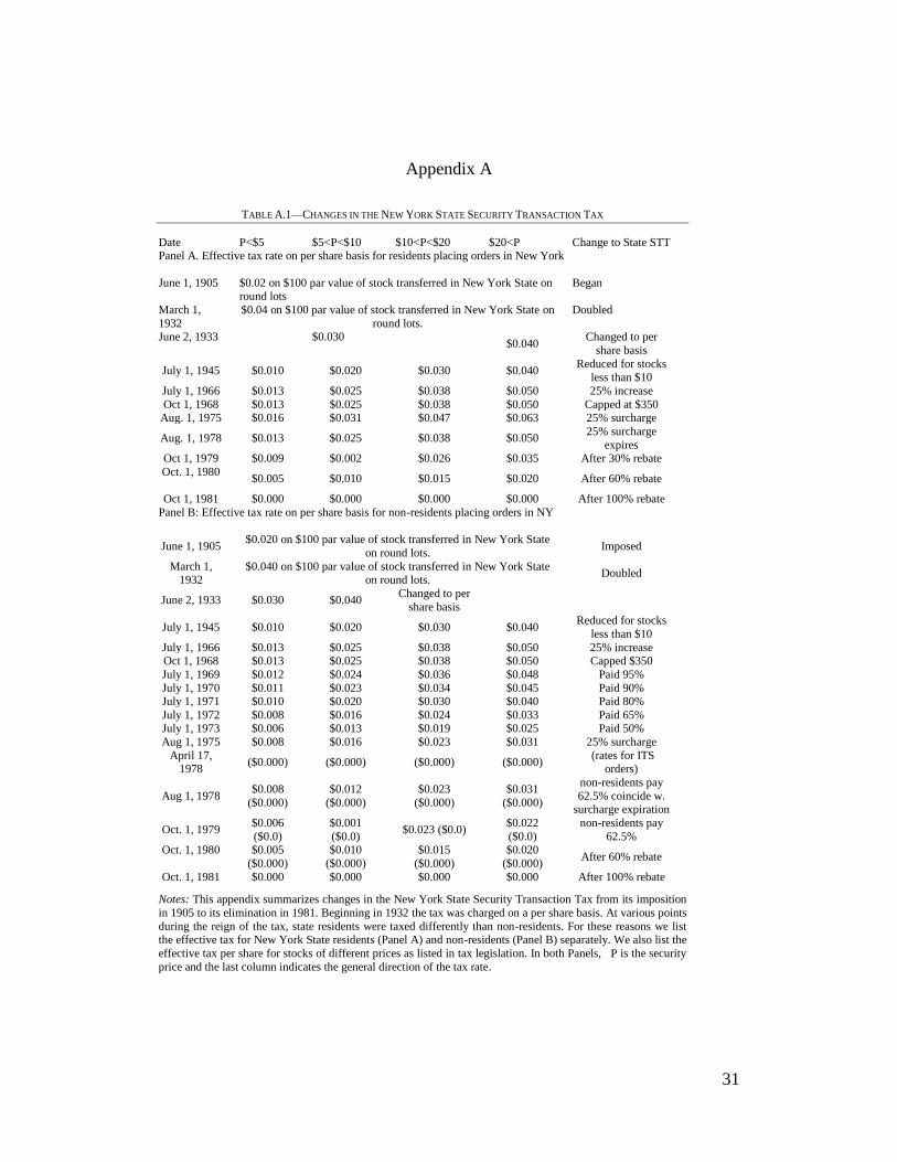
Appendix A illustrates effective transfer tax rates for various stock prices and
partitioned by whether the investor was a New York resident or not.
New York was not the only taxing authority to levy transfer taxes. On
December 1, 1914, the federal government imposed a $0.02 tax on each $100 of
par value of stock to help pay for the cost of US involvement in World War I.
That tax was repealed briefly in September of 1916, but reinstated in December
1917.14
On June 21, 1932 the tax was changed to $0.04 per $100 of par value,
unless the stock was trading above $20 in which case it was $0.05 per $100 of par
value. Stocks without par values were taxed on a per share basis. On September
20, 1941, the tax was increased to $0.05 ($0.06) per $100 of par value for stocks
trading at or below (above) $20 per share. The federal tax was repealed in
January 1966.
Massachusetts and Pennsylvania also levied transfer taxes at one time, but their
impact was much smaller than the New York tax. By 1939 Massachusetts and
13 The intermarket trading system is an electronic linkage system that links together U.S. equity exchanges and 100%
of the tax was rebated on all orders placed through ITS so that the tax would not hinder market competition. As a result,
non-residents could avoid the tax entirely by placing orders through ITS. 14
―Wall St. Sees End of Stock Sales Tax‖, New York Times, July 4, 1916.

8
Pennsylvania levied a tax of two cents per $100 of aggregate par-value of stock
sold or two cents per share in the case of no par-value stock.15
The fact that New
York levied the tax on a per share basis and Massachusetts and Pennsylvania used
aggregate par value resulted in a much higher tax paid in New York.16,17
Corporations could reduce the impact of the tax on their shareholders, by
managing their par values. To investigate this possibility, we obtain par values for
our sample of 236 stocks from the 1932 doubling of the New York tax from the
Moody's Manuals for 1934.18
We find that railroad industry stocks tend to have
par values of $100 (20 out of 27 firms). For the 200 non-railroad industry stocks
covered by Moody's, there were only ten with par values of $100, while 132 listed
no par value and 58 had par values between $1 and $50. We also examine
reported changes in par value around the 1932 New York doubling of their STT.
We find that 28 firms (from our sample of 236) changed their par value between
1930 and 1933. Of these 28 we find that 24 changed to a par value that lowered
taxes based on par.19
Therefore we conclude that firms actively changed their par
values to avoid STTs for their investors. Thus, STTs that are based on share price
cannot be avoided by corporate actions and will have the largest impact on
investors. We would then expect the New York STT to have a measurable impact
on investor behavior and hence market quality.
One purpose of this study is to examine the change in market share across state
lines around transaction tax changes. Since the federal transfer tax could not be
15 Recall that New York switched to taxing on a per share basis much earlier.
16 For example, assume a trade involving 100 shares of a $10 par value stock for $40 a share. The New York tax is $4
($0.04 on each share sold) while the Pennsylvania and Massachusetts tax is $0.20, since the aggregate par-value of the 100 shares is $1,000. It can therefore be seen that the New York tax is 20 times greater than the tax in Massachusetts or
Pennsylvania. See “Stock-Deal Taxes and Their Effects‖, New York Times, December 10, 1939. 17
Both the MA and PA transaction taxes remained inconsequential and were repealed in the 1950s. 18
See Moody's Manual of Investments and Security Rating Service volumes for industrial, bank and financial, public
utility, and railroad securities. 19
Fifteen increased their par value from zero to a small positive number and nine reduced their par to a smaller
number. The remaining four firms reduced their par value to zero.

9
avoided inside the United States and states other than New York imposed a
minuscule tax, we focus on those tax changes occurring in New York. We are
however cognizant of confounding impacts so we are careful to control for
changes in federal tax rates around the time of New York tax changes.
III. Literature Review
Theoretical papers have not reached a consensus on the impact of STTs on
market quality. Some argue that an STT will improve market quality, while
others argue that it will reduce it. Still others state that the effect is ambiguous.
Following is a review of the different camps in this ongoing debate.
The earliest proponents of STTs, Keynes (1936) and Tobin (1978), argue that
an STT will improve market quality. In particular, Keynes contends that chasing
short-term returns, while potentially profitable to some, is a zero-sum game in
terms of economic welfare. Since one investor‘s gain is another's loss and trading
utilizes resources, the value-added through trading is negative. As a result,
imposing an STT may increase welfare by reducing wasted resources. Second,
since trading is speculative by nature, it potentially contributes to financial
instability when trades are driven by short-term capital gains and not fundamental
information. Keynes argues that an STT will curtail short-term speculation, and
thereby reduce wasted resources, market volatility and asset mispricing.
Consistent with Keynes, Tobin (1978) proposes a tax on foreign exchange
transactions that would make short term currency trading unprofitable. He
suggests that a transaction tax would "throw some sand in the wheels of
speculation."
Consistent with these arguments, Stiglitz (1989) and Summers and Summers
(1989) argue that an STT targets short-term noise traders whose trades contribute

10
to excess market volatility. Therefore, an STT is associated with a reduction in
volatility.
Stiglitz (1989) further argues that the impact of an STT on market liquidity
would be insignificant. He contends that although an STT will lead to thinner
markets, the change in spread will be insignificant since the extra time that
market-makers hold securities will not yield a significant change in the inventory
risk component of the spread.
In stark contrast to the proponents of an STT, the opponents argue that an STT
will have an adverse impact on market quality. In particular, Kupiec (1991)
develops a model where an STT is directly related to excess volatility. Similarly,
Amihud and Mendelson (2003) conclude that an STT is directly related to
volatility since STTs reduce the amount of informed trading, thereby widening the
gap between the transaction prices and the security‘s fundamental value.
Schwert and Seguin (1993) suggest that there is no evidence of excess volatility
and since the tax is a burden on all traders, the reduction in trading will not limit
the activity of noise traders alone—it will affect liquidity traders and price-
stabilizing informed traders as well. Therefore, the impact of the tax on volatility
is ambiguous. The authors also argue that an STT would indirectly increase
transaction costs through the three components of the bid-ask spread: order
processing costs, inventory risk and information asymmetry.20
For example, since
an STT reduces trading volume, the number of trades available for the market-
maker to recover his fixed cost declines, thereby increasing the order processing
component of the spread.21
20 The order processing component is part of the fixed cost the market-maker charges for trade execution. The
inventory risk component is the market-maker‘s compensation for holding onto risky assets. The information asymmetry component represents the likelihood that a market-maker is facing an informed trader who has superior knowledge of the
asset‘s fundamental value. 21
An STT will also increase the order processing component directly due to the cost of collecting the tax. Second,
because equity market-makers use derivatives to hedge their risky inventory positions, an STT on derivatives increases the cost of hedging their positions. The increase in the market-maker‘s cost for hedging increases the inventory risk part of the
11
Just as the theoretical literature is divided on the impact of STTs on market
quality, so too is the empirical literature. Apart from Roll (1989), which performs
cross-country regressions, the eleven empirical studies examine 28 different STT
tax (and quasi-tax) changes in 11 different countries. We summarize the empirical
literature in Table 1 and discuss it below. For each paper we list the change in
percentage tax (quasi-tax) for each event since there may be a relationship
between the size of the change and the impact on volatility. We also list for each
paper the measures examined in the paper as well as the finding for each measure.
Statistically significant findings are indicated by an asterisk, otherwise the finding
is insignificant. Rather than discussing each paper separately we will focus on the
findings for each measure of market quality examined.
A. Volatility
Of the nine papers that empirically examine changes in volatility around
changes in STTs, only one (Roll (1989)) finds the inverse relationship predicted
by Stiglitz (1989) and Summers and Summers (1989). That relationship is,
however not significant. Two of the papers (Baltagi, Li, and Li (2006) and Jones
and Seguin (1997)) find a statistically significant direct relationship between
volatility and the level of an STT which supports the predictions of Kupiec (1991)
and Amihud and Mendelson (2003). The remaining papers either find an
insignificant direct relationship (Umlauf (1993) and Hau (2006)) or conclude that
they find no relationship.
bid-ask spread. Finally, if an STT reduces the amount of noise trading, as proponents suggest, then the possibility of the
market-maker facing an informed trader increases, thereby increasing the information asymmetry element of the bid-ask spread.

12
B. Volume
Each of the five studies that examine the relationship between volume and an
STT find evidence of an inverse relationship. Baltagi, Li, and Li (2006) find a
statistically significant relationship while the remaining papers (Hu (1998), Liu
(2007) Sahu (2008) and Jarrell (1984)) report an insignificant inverse
relationship.22
These papers support the theoretical predictions of an inverse
relationship argued by Schwert and Seguin (1993). A complementary measure
related to volume used in the literature is market share. For example, Campbell
and Froot (1994) point out that in many cases domestic investors can avoid STTs
by trading in another country. Consistent with Campbell and Froot, Umlauf
(1993), finds that an increase in a securities transaction tax is associated with a
decline in market share in the domestic country. Existing studies may not be able
to capture the true level of volume transferred between exchanges due to currency
risk concerns as well as the lack of fungibility existing across borders.
C. Spreads
Prior to this study there has been a lack of empirical evidence of the impact of
an STT on spread. The literature on the impact of stock transaction taxes on
spreads largely relies on the indirect effect of trading volume on liquidity.
Bloomfield, O‘Hara and Saar (2009) examine the relationship between spreads
and STTs in a laboratory setting in the context of different types of traders. They
examine three scenarios for the impact of an STT on the components of bid-ask
spread. If noise traders are less active because of the STT, the inventory risk
component of the spread may decrease; the adverse selection cost may increase;
22 Jarrell (1984) does not conduct tests of significance.

13
or it may remain unchanged. If noise traders trade less, then prices will be less
volatile and the inventory risk component of the bid-ask spread will decline,
thereby increasing liquidity. However, if noise traders trade less, increasing the
probability of informed trading, then the adverse selection costs could increase,
resulting in a increase in spreads. Finally, given a decline in noise trading from
an STT, informed traders may trade less aggressively on their information,
keeping adverse selection costs unchanged. Bloomfield, O‘Hara and Saar (2006)
use the total price impact as a proxy for spreads and find no significant effect on
spreads or price impact.
The empirical literature does not reach a consensus. By empirically examining
nine changes in the level of an STT in the same market with market share not
being clouded by fungibility, this paper adds to the empirical literature on STTs.
IV. Data and Methodology
We obtain dates for changes in the level of security transaction taxes at the state
and federal level from the New York Times and Wall Street Journal. As stated
earlier, in addition to the federal stock transfer tax instituted in 1914, the states of
New York, Massachusetts, and Pennsylvania all enacted STTs during the last
century. As previously shown, the Massachusetts and Pennsylvania taxes were
minuscule so they are ignored. Since one goal of this paper is to examine whether
traders move their trading to avoid taxes, we do not examine the nationwide
federal tax. We then focus on changes in the New York STT from its imposition
in 1905 through its elimination in 1981. The dates and tax rates are contained in
Appendix A. There are eleven tax changes that impact both residents and non-
residents. The October 1, 1968 tax change placed a cap of $350 on the tax paid for
one transaction. The cap impacted trades of over 7,000 shares for prices above
$20 and trades of over 28,000 shares for prices less than $5. Since this was

14
limited to larger trades we would not expect a market wide change in market
quality and thus do not examine that change.
We use daily closing prices and volume to estimate the impact of an STT on
volatility, spreads and price impact. Daily closing prices and volume for the
NYSE, American Stock Exchange (AMEX) and National Association of
Securities Dealers Automated Quotations (NASDAQ) are obtained from the
Center for Research in Security Prices (CRSP). The CRSP databases do not
contain prices prior to 1925; therefore due to data limitations we are not able to
examine the imposition of the New York STT in 1905. We then limit our study to
the nine remaining tax changes that impact both residents and non-residents.
Consistent with Jones and Seguin (1997), we define sample stocks as all those
continuously traded on the two New York stock exchanges - the NYSE and
AMEX from one year before to one year after each tax change. There are four
exceptions to this rule due to the proximity of confounding events. The March
1932 New York increase occurs just three months before the June 1932 doubling
of the federal STT. As stated earlier, corporations managed the STT paid by their
investors by changing their par values. We hypothesize that changing the New
York STT to a per share basis (June 1933) will have a larger impact on market
quality than doubling the amount taxed on par value at both the New York (March
1932) and Federal (June 1932) level. To test this hypothesis we use the twelve
months before the March 1932 New York event and the eleven months June 1932
through May 1933 as the post period. For the July 1966 New York state tax
increase, six months pre and post are used to avoid a confounding influence
related to the January 1966 elimination of the federal security transaction tax.
Similarly, fixed commissions (a quasi-transaction tax) were abolished three
months prior to the August 1975 STT increase. Therefore, the 1975 event uses
three months pre and post. Finally, the August 1, 1978 tax change coincides with
the introduction of the Intermarket Trading System. A pilot program of 11 stocks

15
traded on the NYSE and Philadelphia Stock Exchange began in April 1978.
Between August and November 1978 the program was expanded to include all
inter-listed stocks on multiple regional exchanges. The 1978 tax change gives
orders placed through ITS (and destined for the NYSE) a 100% rebate. To avoid
confounding influences of the ITS start up period, we define the post period for
the 1978 tax change as December 1978 through June 1979.
In their study of the elimination of fixed commissions, Jones and Seguin (1997)
employ NASDAQ stocks as a control sample. During the period of our study,
NASDAQ's headquarters was in Washington, DC. Many of the stocks listed on
NASDAQ were similarly headquartered outside of New York and therefore stock
transfers took place outside of New York as well. Finally many NASDAQ traders
were not residents of New York. For these reasons a large portion of the trading
occurring on NASDAQ was not subject to the New York STT. Therefore, we
adopt the methodology of Jones and Seguin and use NASDAQ firms as a control
sample.23
Since CRSP data are not available for NASDAQ prior to 1972, we can
only employ this control sample for tax changes from 1975 on.
The market quality measure that has garnered the most attention in theoretical
and empirical papers is volatility. Following Jones and Seguin (1997) we adopt a
portfolio approach rather than examining individual securities. Jones and Seguin
argue that the portfolio approach is superior to examining single stocks since most
investors hold portfolios and measuring portfolios removes measure bias due to
microstructure effects such as the bid-ask bounce. The portfolios consist of either
all the NYSE/AMEX stocks or all of the NASDAQ stocks. Volatility is defined as
the standard deviation of continuously compounded daily returns for the period
before (pre ) and the period after (
post ) a change in the level of STT. We then
23 Consistent with Jones and Seguin (1997) any NASDAQ stock with a market value less than the smallest
NYSE/AMEX firm is excluded.

16
specify the change in volatility aspost pre . For each day t over the
estimation period we calculate the equally weighted return for portfolio p
(NYSE/AMEX or NASDAQ), Rpt. To estimate σpre and σpost we follow Johnson
and Kotz (1970) (as well as Jones and Seguin (1997)) and estimate the standard
deviation of each portfolio p by multiplying the mean absolute value of returns by
2
, where π is the mathematical constant.
24
Table 2 reports cross-sectional means of market values, stock prices, and our
daily return standard deviation measure of volatility based on continuously
compounded returns for NYSE/AMEX and NASDAQ stocks for each tax change.
For NYSE/AMEX stocks we observe that the average price is fairly stable over
the entire sample period. We also note that volatility is fairly stable around each
NYSE/AMEX STT change from 1945 on. For the NASDAQ stocks we observe
that the firms are smaller than NYSE/AMEX firms and exhibit lower average
prices than those of the NYSE/AMEX. Note that our sample of NASDAQ stocks
has lower average volatility than the NYSE/AMEX sample. This is consistent
with the findings of Jones and Seguin (1997).
To obtain an estimate of the change in volatility following a tax change, we
regress the standard deviation of each portfolio on a dummy variable IPost,t which
takes the value 1 if the day is after the tax change, otherwise zero or,
(1) 𝜋
2 𝑅𝑝 ,𝑡 = 𝛽𝑝0 + 𝛽𝑝1𝐼𝑝𝑜𝑠𝑡 ,𝑡 + 𝜀𝑝 ,𝑡 ,
where βp0 then represents an estimate of the pre-event volatility and βp1 represents
the change in volatility from the pre-event. Newey-West standard errors with five
lags are reported for the volatility change βp1. More specifically, we estimate:
24 See Johnson and Kotz (1970).

17
𝜋
2 𝑅𝑝 ,𝑡
𝑁𝑌 = 𝛽𝑝 ,0𝑁𝑌 + 𝛽𝑝 ,1
𝑁𝑌𝐼𝑝𝑜𝑠𝑡 ,𝑡 + 𝜀𝑝 ,𝑡𝑁𝑌 ,
(2) 𝜋
2 𝑅𝑝 ,𝑡
𝑁𝐴𝑆𝐷 = 𝛽𝑝 ,0𝑁𝐴𝑆𝐷 + 𝛽𝑝 ,1
𝑁𝐴𝑆𝐷𝐼𝑝𝑜𝑠𝑡 ,𝑡 + 𝜀𝑝 ,𝑡𝑁𝐴𝑆𝐷 ,
𝑐𝑜𝑣 𝜀𝑝 ,𝑡 𝑁𝑌 , 𝜀𝑝 ,𝑡
𝑁𝐴𝑆𝐷 = 𝑣,
𝑐𝑜𝑣 𝜀𝑝 ,𝑠 𝑁𝑌 , 𝜀𝑝 ,𝑡
𝑁𝐴𝑆𝐷 = 0 ∀ 𝑠 ≠ 𝑡.
The methodology described above does not account for differing volatility
levels across the two markets. To control for unequal variances we follow
Schwert and Seguin (1990) and model conditional heteroskedasticity for a
portfolio as being linear in the predicted standard deviation of some aggregate
portfolio factor.25
We specify the NYSE/AMEX firms as a function of the
NASDAQ portfolio conditional on volatility. Given that NASDAQ transactions
were largely not affected by New York State transfer taxes, we use the NASDAQ
portfolio as a proxy for the single volatility factor.
Specifically, we first obtain the fitted value of daily NASDAQ portfolio return
standard deviation by regressing the standard deviation of returns on the size-
relevant NASDAQ portfolio at time t onto 12 lags of daily returns. That is,
(3) 𝜎𝑝𝑡𝑁𝐴𝑆𝐷 = 𝛽0 + 𝛽𝑖𝜎𝑝𝑡−𝑖
𝑁𝐴𝑆𝐷 + 𝜇𝑝𝑡12𝑖=1 ,
where 𝜎𝑝𝑡𝑁𝐴𝑆𝐷 is the absolute value of returns to the NASDAQ portfolio multiplied
by 𝜋2 . We then use the fitted values in the following regression,
(4) 𝜎𝑝𝑡𝑁𝑌 = 𝛾0 + 𝛾1𝜎 𝑝𝑡
𝑁𝐴𝑆𝐷 + 𝛾2𝜎 𝑝𝑡𝑁𝐴𝑆𝐷 𝐼𝑝𝑜𝑠𝑡 ,𝑡 + 𝜀𝑝𝑡 ,
25 Schwert and Seguin (1990) find that a single-factor model of standard deviations describes the cross sectional and
time series characteristics of portfolio volatility as well as a GARCH model, and better than a linear variance-based specification.

18
where 𝜎𝑝𝑡𝑁𝑌 is the standard deviation of a NYSE portfolio p at time t estimated as
the absolute value of the return to the portfolio multiplied by / 2 ; ,POST tI is a
dummy variable, taking on the value 0 for the pre-event period and 1 for the post
event time frame; 𝜎 𝑝𝑡𝑁𝐴𝑆𝐷 is the estimated standard deviation of returns on the size-
relevant NASDAQ portfolio at time t, conditional on 12 lags of daily returns. The
parameter estimate γ1 then measures the level of NYSE/AMEX volatility relative
to NASDAQ volatility.
To capture the effect of the STT change on volatility, we specify an interaction
variable between the dummy and the NASDAQ portfolio standard deviation
variable, 𝜎 𝑝𝑡𝑁𝐴𝑆𝐷 𝐼𝑝𝑜𝑠𝑡 ,𝑡 . This allows for the measurement of changes in volatility
of our NYSE/AMEX sample firms as a result of a tax change, while using
NASDAQ firms to control for conditional heteroskedasticity. Therefore, the
parameter estimate γ2 measures changes in the proportional level of
NYSE/AMEX volatility. However, due to lack of data availability, we can only
apply this methodology to events from 1972 on.
The next market quality measure we examine is spread width. This measure has
not been previously examined in the extant literature. However, bid and ask data
is not available for US stocks prior to the 1990s. Recently Holden (2009) has
developed a low frequency proxy for effective spread width that Goyenko,
Holden, and Trzcinka (2009) show provides good estimates of actual effective
spread. Following Holden (2009) we use the frequency with which closing prices
occur in particular price clusters, to estimate the corresponding spread
probabilities.26
Two other market quality variables of interest are volume and market share for
exchanges in and out of New York around each tax change. Traders can switch
26 Estimation of the Holden (2009) effective spread is available from the authors upon request.

19
their trading to an exchange outside of New York to avoid the New York STT if
that opportunity exists. However, for the majority of our sample period, shares
were traded in physical form so it was necessary for brokers and transfer agents to
be close to each other to transfer actually securities. As a result, it was more
difficult for investors to avoid the tax. In addition, while many NYSE stocks
were traded on regional exchanges outside of New York, American Stock
Exchange stocks were not. Therefore, we limit this part of the study to NYSE
stocks. If traders do indeed switch to non-NYSE venues to avoid the tax then we
should see a reduction in the NYSE's market share and volume following tax
increases and an increase following tax reductions. To obtain the needed data, we
hand collect monthly volume figures from the Bank and Quotation Record for
each regional exchange as well as the NYSE. Market share is estimated as the
total trading volume for each exchange in month t divided by the total sum of
volume on all exchanges. That is,
(5) 𝑚𝑎𝑟𝑘𝑒𝑡𝑠ℎ𝑎𝑟𝑒𝑥 ,𝑡 = 𝑣𝑜𝑙𝑢𝑚𝑒 𝑥 ,𝑡
𝑣𝑜𝑙𝑢𝑚𝑒 𝑥 ,𝑡𝑛𝑥=1
,
where x represents the total volume on exchange x in month t. To calculate
impacts we average market share for each exchange over either the pre or post
period.
The final market quality measure we examine is price impact. If an STT reduces
volume then we would expect trades to have larger price impact, ceteris paribus.
Again, due to data limitations during the period of our study we rely on low-
frequency proxies for price impact. We rely on the Amihud (2002) price impact
measure which has been shown by Goyenko, Holden and Trzcinka (2009) to be a
good proxy for price impact. Specifically, Amihud‘s illiquidity proxy is measured
as
20
(6) 𝐴𝑚𝑖ℎ𝑢𝑑 = |𝑟𝑖 ,𝑡 |
$𝑉𝑜𝑙𝑢𝑚𝑒 𝑖 ,𝑡,
where ri,t and $Volumei,t are the stock return and dollar volume for stock i on day
t, respectively. This ratio can be interpreted as the daily price impact of order
flow because it measures absolute price change per dollar of daily trading volume.
In the next section we discuss the results of tests to measure changes in our
market quality measures around STT changes.
V. Results
The first market quality measure we examine is volatility. Recall that
proponents of an STT argue that the imposition or increase in the tax will reduce
speculation and hence volatility. Therefore they predict an inverse relationship
between an STT and volatility. However, only one (Roll (1989)) of the nine
empirical papers cited in Table 1 that examine volatility finds evidence of an
inverse relationship as predicted by proponents of the tax.27
All but one of the
remaining papers finds no statistically significant relationship, while Jones and
Seguin (1997) find a statistically significant direct relationship between the tax
and volatility. We use the methodology of Jones and Seguin to examine the
relationship between volatility and nine changes in the level of the New York
State STT between 1932 and 1981.
The results of our regressions are found in Table 3. Panel A reports the date and
nature of each change in the first column. The next column lists the percentage
point change in the STT for a $5 stock. The remaining columns show the
parameter estimates for each change for stocks listed on the New York and
American stock exchanges. The parameter estimate of interest is βp1 which
measures the change in volatility following the change in the STT. Examining the
27 Only nine of the ten papers examine volatility. Liu (2007) does not.
21
parameter estimates in column four reveals that in five instances volatility
appeared to change in the direction of the tax change (1932, 1933, 1966, 1980,
and 1981) while the level of volatility appears to move in the opposite direction of
the tax change for four of the events (1945, 1975, 1978, and 1979). Only four of
the nine estimates are statistically significant at acceptable levels and there is no
consistent pattern among these four estimates.
It may very well be that the observed changes in volatility are the result of
market wide changes in volatility unrelated to changes in the STT rate. To test for
this we employ NASDAQ stocks as a control group. Since NASDAQ was located
in Washington DC it was not subject to the tax on listed stocks. In addition,
brokers and residents of states outside of New York were likewise exempt from
the New York STT for stocks incorporated outside of New York. NASDAQ data
are only available starting in 1975.28
Comparing the NASDAQ parameter
estimates in column six to their counterparts for NYSE/AMEX stocks reveals that
in all five comparisons, NASDAQ stock volatility changed in a direction similar
to NYSE/AMEX stocks. Further four of the five NASDAQ parameter estimates
are statistically significant suggesting that there may indeed have been market
wide changes in volatility unrelated to the change in the STT. We test whether the
NYSE/AMEX and NASDAQ parameter estimates are statistically similar using a
Wald test. The Wald p values are listed in the last column of Panel A in Table 3.
The p values suggest that the parameter estimates for NYSE/AMEX and
NASDAQ are statistically indistinguishable providing further evidence that the
observed changes in volatility are related to market wide changes and not changes
in the STT. Taken together, the results reported in Panel A agree with the majority
28 Prior to 1975, trading occurred when brokers contacted other brokers who were listed as trading a stock on the Pink
Sheets. Quotes on the Pink Sheets were often stale and therefore closing prices were impossible to estimate. Beginning in
1975, NASDAQ automated the Pink Sheets for a large number of stocks and allowed for contemporaneous quote updating.
Closing prices were based on the midpoint of the closing spread until 1980. At that time, NASDAQ market makers began reporting their trades contemporaneously and closing prices could therefore be determined.

22
of the empirical papers listed in Table 1. There appears to be no statistically
significant relationship between the level of an STT and volatility.
In Panel A we examine the absolute changes in volatility. However, this may
not be appropriate measure of volatility if volatility varies across the
NYSE/AMEX and NASDAQ portfolios. Therefore, in Panel B we present results
for proportional changes in volatility. The first two columns in Panel B list the
date and event tested and the percent change in the STT for a $5 stock. The next
three columns list the parameter estimates, followed by the R2 in the last column.
The parameter of interest is 𝛾2 which measures the proportional change in
NYSE/AMEX volatility relative to NASDAQ following a change in the STT. For
four (1975, 1979, 1980, 1981) of the five events examined in Panel B,
NYSE/AMEX volatility moves in the same direction as the STT change,
however, only one parameter estimate is statistically significant. In particular,
for the 1979 event, NYSE/AMEX volatility is on average 93% of NASDAQ
volatility before the 30% rebate, but falls to 85% (0.927 - 0.076) of NASDAQ
volatility after the STT decline. Thus, the results reported in Panel B agree with
our previous findings, in that there appears to be no consistent statistically
significant relationship between the level of an STT and volatility.
The next market quality measure we examine is spread width. This measure has
not been previously examined in the extant literature. Since bid and ask data is not
available for US stocks prior to the 1990s, we employ the Holden low frequency
measure described in Holden (2009). We first examine univariate changes in
spread width surrounding our STT events. The pre-event, post-event, and change
in spread are listed in Panel A of Table 4. Only NYSE and AMEX stocks are
included in this table.29
Examining the average change in spread and comparing it
to the change in STT reveals that in all cases spread width changed in the
29 Due to data limitations we are unable to compute the Holden proxy for Nasdaq firms. Specifically, CRSP does not
report Nasdaq volumes prior to the 1980s.

23
direction of the STT. In all but one case, the change is statistically significant at
acceptable levels.
The changes in spread reported in Panel A may be the result of changes in other
variables known to be associated with spread width. Accordingly we perform
control regressions of the form
(7) 𝐻𝑜𝑙𝑑𝑒𝑛𝑖,𝑡 =
𝛽0 + 𝛽1𝑉𝑜𝑙𝑖,𝑡 + 𝛽2𝜎𝑖,𝑡 + 𝛽3𝐷𝑢𝑚𝑚𝑦𝑖 ,𝑡 + 𝜀𝑖 ,𝑡 ,
where Vol is traded volume for stock i on day t, σ is measured by / 2 ptR , and
Dummy takes the value 0 pre-event and 1 post-event. The parameter estimates of
the control regression are found in Panel B of Table 4. Consistent with previous
literature the parameter estimate for volume is mostly negative and that for
volatility positive. The parameter of interest is 𝛽3. Examining the estimates, only
in one of the nine cases is the observed sign of the Dummy estimate of the
opposite sign of the STT change. However, in the parameter estimate is not
significant. Of the eight remaining cases where the parameter estimate and STT
are of the same sign, six are statistically significant at acceptable levels. Based on
the univariate and multivariate evidence in Table 4, we conclude that an STT has
a direct relationship with spread width. That is, imposing or increasing an STT
will be associated with wider spreads. For both the univariate and multivariate
tests, consistent with our hypothesis, the 1933 event exhibits a larger change in
spread than the 1932 event, indicating that per share taxes result in larger market
quality changes than par value tax changes since the latter can be managed by
corporations through par value changes.
Given the inverse relationship between spread width and volume documented in
previous literature, and given that we find spreads to have a significant direct
24
relationship with changes in STT levels, we would also expect volume to have an
inverse relationship. Of the five papers listed in Table 1 that examine volume, all
five find an inverse relationship between an STT and volume, but only one is
statistically significant. Accordingly, we next examine volume. We must
remember though that the STT changes we examine only impact New York State
exchanges, corporations, and residents. Therefore we expect the impact of
changes in the level of the New York STT to mostly impact New York
exchanges. We must also remember that in some circumstances non-New York
investors could avoid the tax by trading on exchanges outside of NY. Changes in
STTs may induce those that can to switch trading to another exchange. Umlauf
(1993) documents that the increase in Swedish transaction taxes in 1986 is
associated with a dramatic shift in trading from Stockholm to London.
We therefore examine both market share and volume for the NYSE and
regional exchanges in Table 5. Listed is the average market share and monthly
share volume for each exchange before and after each New York STT change.
During the time period of our study (1932-1981) an increasing portion of regional
stock exchange volume was in NYSE listed stocks.30
Therefore, we expect that
regional stock exchange market share would increase (decrease) when New York
State increases (decreases) the level of the STT. However, because the New York
State tax was applied as long as part of the transaction took place within the state
(i.e. if the location of the exchange, contra broker or transfer agent is in New York
or if the stock seller is domiciled in New York) and most brokers and transfer
agents were located in New York, it may have been difficult for investors to shift
their trading and avoid the STT. We find that for five of the nine STT changes
(1933, 1945, 1966, 1975, and 1978) the sign of NYSE market share change was
30 See Weaver (2008) for a discussion of the changing role of regional stock exchanges in the 20th Century.

25
opposite that of the STT sign change, and in four cases it was of the same sign.
Therefore, our results are mixed.
Some investors may not switch to (from) a regional exchange if there is an
increase (decrease) in the New York STT. Some may just not trade certain stocks.
Therefore, we also look at volume since it captures volume switched to other
exchanges as well as decisions to not trade at all. Examining NYSE volume in the
last three columns of Table 5 reveals that, in eight of the nine STT changes,
volume moved in the opposite direction of the tax change. Six of those eight cases
are statistically significant at acceptable levels. Therefore we conclude that,
consistent with previous empirical papers, STTs and volume are inversely related.
Since trading volume acts as a shock absorber for price impacts, we would also
expect that changes in STT levels would affect measures of price impact. We
examine that possibility by considering the Amihud measure. An increase in the
Amihud measure indicates a decrease in liquidity in that a given volume will have
a larger price impact. A direct relationship between the Amihud measure and
changes in the STT would suggest that STTs harm market quality, while an
inverse relationship would suggest that it improves it. Table 6 provides univariate
changes in the Amihud measure surrounding STT level changes. Examining the
change in the Amihud measure after the STT changed reveals that for seven of the
nine STT changes the Amihud measure changed in the direction of the tax change
and that all seven cases are statistically significant at acceptable levels. This
suggests that STTs adversely impact market quality.
VI. Conclusion
Security transaction taxes have been the subject of debate for decades among
academics that develop models of the relationship between STTs and market
quality, empiricists who examine the relationships for existing taxes, and

26
governments seeking to raise revenue without harming economic growth. In spite
of the length of the debate, no consensus has yet been reached. We add to the
debate by examining the impact on market quality of nine changes to the New
York State STT between the first significant change to it in 1932 and its repeal in
1981.
We find that increasing an STT is accompanied by an increase in transaction
costs for investors, a reduction in volume, and higher price impact for trades. We
find no consistent relationship that suggests that investors will switch trading to
non taxing venues to avoid the tax, but do find that corporations will manage par
values in the direction of minimizing taxes if they are based on par value. Finally,
we find no support for the notion that STTs reduce volatility.
Our findings largely come down on the side of opponents of the tax who
suggest that an STT will harm market quality. Since spreads have been shown to
be directly related to a firm's cost of capital, imposing an STT may hinder
economic growth by reducing the present value of projected profits.
REFERENCES
Amihud, Yakov. 2002. ―Illiquidity and stock returns: cross-section and time-
series effects.‖ Journal of Financial Markets, 5: 31–56.
Amihud, Yakov and Haim Mendelson. ―Transaction Taxes and Stock Values.‖ In
Modernizing U.S. Securities Regulations: Economic and Legal Perspectives,
edited by Robert W. Kamphuis, Jr., 477-500. New York: Irwin Professional
Publishing, 1992.

27
Amihud, Yakov and Haim Mendelson. 2003. ―Effects of a New York State Stock
Transaction Tax.‖ Unpublished.
Aristidou, Antonis A. and Kate Phylaktis. 2007. ―Security Transaction Taxes and
Financial Volatility: Athens Stock Exchange.‖ Applied Financial Economics,
17(18): 1455-1467.
Baltagi, Badi H., Dong Li and Qi Li. 2006. ―Transaction Tax and Stock Market
Behavior: Evidence from an Emerging Market.‖ Empirical Economics, 31:
393–408.
Bloomfield, Robert, Maureen O‘Hara and Gideon Saar. 2009. ―How Noise
Trading Affects Market: An Experimental Analysis.‖ Review of Financial
Studies, 22(6): 2275–2302.
Campbell, John Y. and Froot, Kenneth A. ―International Experiences with
Securities
Transaction Taxes.‖ In The internationalization of equity markets, edited by
Jeffrey Frankel, 277-308. Chicago: University of Chicago Press, 1994.
Christie, William G., and Paul H. Schultz. 1994. ―Why do NASDAQ market
makers avoid odd-eighth quotes?‖ Journal of Finance, 49: 1813–1840.
Goyenko, Ruslan Y., Craig W. Holden and Charles Trzcinka. 2009. ―Do liquidity
measures measure liquidity?‖ Journal of Financial Economics, 92: 153-181.
Hau, Harold. 2006. ―The Role of Transaction Costs for Financial Volatility:
Evidence from the Paris Bourse.‖ Journal of the European Economic

28
Association, 4(4): 862–90.
Holden, Craig W. 2009. ―New low-frequency liquidity measures.‖ Journal of
Financial Markets, 12: 778 – 813.
Hu, Shing-yang. 1998. ―The Effects of the Stock Transaction Tax on the Stock
Market—Experience from Asian Markets.‖ Pacific Basin Finance Journal, 6:
347–64.
Huang, Roger D. And Hans R. Stoll. 1997. ―The components of the bid–ask
spread: a general approach.‖ Review of Financial Studies, 10: 995–1034.
Jarrell, Gregg A. 1984. "Change at the Exchange: The Causes and Effects of
Deregulation." Journal of Law and Economics, 27(2): 273-312.
Johnson, Norman L. and Samuel Kotz. Continuous Univariate Distributions.
Boston: Houghton Mifflin, 1970.
Jones, Charles M. and Paul Seguin. 1997. ―Transaction costs and price volatility:
Evidence from commission deregulation.‖ American Economic Review, 87:
728-37.
Liu, Shinhau. 2007. ―Securities Transaction Tax and Market Efficiency: Evidence
from the Japanese Experience.‖ Journal of Financial Services Research, 32:
161–76.
Keynes, John M. The General Theory of Employment, Interest and Money.

29
London: MacMillan, 1936.
Kupiec, Paul H. 1991. ―Noise Traders, Excess Volatility, and a Securities
Transaction Tax.‖ Finance and Economics Discussion Series 166.
Roll, Richard. 1989. ―Price volatility, international market links, and their
implications for regulatory policies.‖ Journal of Financial Services Research, 3:
211-46.
Sahu, Dhananjay. 2008. ―Does Securities Transaction Tax Distort Market
Microstructure? Evidence from Indian Stock Market.‖
http://papers.ssrn.com/sol3/papers.cfm?abstract_id=1088348
Saporta, Victoria. and Kamhon Kan. 1997. ―The effects of stamp duty on the level
and volatility of UK equity prices.‖ Bank of England Working Paper 71.
Schwert, G. William, and Paul J. Seguin.1990. ―Heteroskedasticity in Stock
Returns.‖ Journal of Finance, 45: 1129-1155.
Schwert, G. William, and Paul J. Seguin. ―Securities Transaction Taxes: An
Overview of Costs, Benefits and Unresolved Questions.‖ Financial Analysts
Journal, 27–35.
Stiglitz, Joseph E. 1989. ―Using tax policy to curb speculative short-term
trading.‖ Journal of Financial Services Research, 3: 101-15.
Summers, Lawrence H. and Victoria P. Summers. 1989. ―When financial markets
work too well: a cautious case for a securities transaction tax.‖ Journal of

30
Financial Service Research, 3: 261-86.
Tobin, James. 1978. ―A proposal for international monetary reform.‖ Eastern
Economic Journal, 4: 153—59.
Umlauf, Steven R. 1993. ―Transaction taxes and the behaviour of the Swedish
stock market.‖ Journal of Financial Economics, 33: 227-40.
Weaver, Daniel G. ―Networks, Nodes, and Priority Rules‖, In The Encyclopedia
of Finance, edited by Cheng-few Lee and Alice C. Lee, Springer Publishing.
2008.
Zelinsky, Edward. 2002. ―Restoring Politics to the Commerce Clause: The Case
for Abandoning the Dormant Commerce Clause Prohibition on Discriminatory
Taxation.‖ Cardozo Law School Legal Studies Research Paper Series 56.
31
Appendix A
TABLE A.1—CHANGES IN THE NEW YORK STATE SECURITY TRANSACTION TAX
Date P<$5 $5<P<$10 $10<P<$20 $20<P Change to State STT Panel A. Effective tax rate on per share basis for residents placing orders in New York
June 1, 1905 $0.02 on $100 par value of stock transferred in New York State on round lots
Began
March 1,
1932
$0.04 on $100 par value of stock transferred in New York State on
round lots.
Doubled
June 2, 1933 $0.030 $0.040
Changed to per
share basis
July 1, 1945 $0.010 $0.020 $0.030 $0.040 Reduced for stocks
less than $10
July 1, 1966 $0.013 $0.025 $0.038 $0.050 25% increase
Oct 1, 1968 $0.013 $0.025 $0.038 $0.050 Capped at $350 Aug. 1, 1975 $0.016 $0.031 $0.047 $0.063 25% surcharge
Aug. 1, 1978 $0.013 $0.025 $0.038 $0.050 25% surcharge
expires Oct 1, 1979 $0.009 $0.002 $0.026 $0.035 After 30% rebate
Oct. 1, 1980
$0.005 $0.010 $0.015 $0.020 After 60% rebate
Oct 1, 1981 $0.000 $0.000 $0.000 $0.000 After 100% rebate
Panel B: Effective tax rate on per share basis for non-residents placing orders in NY
June 1, 1905 $0.020 on $100 par value of stock transferred in New York State
on round lots. Imposed
March 1, 1932
$0.040 on $100 par value of stock transferred in New York State on round lots.
Doubled
June 2, 1933 $0.030 $0.040 Changed to per
share basis
July 1, 1945 $0.010 $0.020 $0.030 $0.040 Reduced for stocks
less than $10
July 1, 1966 $0.013 $0.025 $0.038 $0.050 25% increase Oct 1, 1968 $0.013 $0.025 $0.038 $0.050 Capped $350
July 1, 1969 $0.012 $0.024 $0.036 $0.048 Paid 95%
July 1, 1970 $0.011 $0.023 $0.034 $0.045 Paid 90% July 1, 1971 $0.010 $0.020 $0.030 $0.040 Paid 80%
July 1, 1972 $0.008 $0.016 $0.024 $0.033 Paid 65% July 1, 1973 $0.006 $0.013 $0.019 $0.025 Paid 50%
Aug 1, 1975 $0.008 $0.016 $0.023 $0.031 25% surcharge
April 17, 1978
($0.000) ($0.000) ($0.000) ($0.000) (rates for ITS
orders)
Aug 1, 1978 $0.008
($0.000)
$0.012
($0.000)
$0.023
($0.000)
$0.031
($0.000)
non-residents pay
62.5% coincide w. surcharge expiration
Oct. 1, 1979 $0.006
($0.0)
$0.001
($0.0) $0.023 ($0.0)
$0.022
($0.0)
non-residents pay
62.5% Oct. 1, 1980
$0.005
($0.000)
$0.010
($0.000)
$0.015
($0.000)
$0.020
($0.000) After 60% rebate
Oct. 1, 1981 $0.000 $0.000 $0.000 $0.000 After 100% rebate
Notes: This appendix summarizes changes in the New York State Security Transaction Tax from its imposition
in 1905 to its elimination in 1981. Beginning in 1932 the tax was charged on a per share basis. At various points
during the reign of the tax, state residents were taxed differently than non-residents. For these reasons we list the effective tax for New York State residents (Panel A) and non-residents (Panel B) separately. We also list the
effective tax per share for stocks of different prices as listed in tax legislation. In both Panels, P is the security
price and the last column indicates the general direction of the tax rate.

32
TABLE 1—SUMMARY OF RESULTS OF PREVIOUS EMPIRICAL PAPERS
Sahu (2008) India 2004 0.0 0.15% Volume - Inverse
Volatility - No relationship
Phylaktis and
Aristidou (2007)
Athens Stock
Exchange
1998 0.0 0.3%
Price Levels - No relationship
Volatility - no impact in
"normal" economic conditions, but direct
relationship during bull
markets
1999 0.3% 0.6%
2000 0.6% 0.3%
Panel B. Changes in Quasi-STT
Jarrell (1984) USA 1975 Deregulation of fixed
commissions Up to 1% Volume - Inverse
Jones and
Seguin (1997) USA 1975
Deregulation of fixed
commissions Up to 1% Volatility - Direct*
Hau (2006) France 2004 Increases in transaction costs Volatility - Direct
Notes: This table summarizes the results of empirical papers that examine the relationship between Security
Transaction Taxes (STT) and the quality of equity markets. All but one of the papers examines changes in the STT or quasi STT. For each paper we list the country examined, the STT change year, and the change. The last
Colum lists the market quality measures considered and the reported relationship with the STT change. If the
relationship is found to be statistically significant, it is indicated by an asterisk (*). Panel A lists those papers that examine STTs while Panel B lists those papers that examine quasi STTs.
Panel A. Changes in STT
Paper Country Year(s) Change
From
Change
to
Measures Examined and
Finding
Umlauf
(1993) Sweden
1984 0% 1% Volatility - Direct Price Levels - Inverse
Market Share - Inverse 1986 1% 2%
Baltagi, Li
and Li (2006) China 1997 0.3% 0.5%
Volume - Inverse*
Volatility - Direct*
Hu (1998)
Hong Kong
1991 0.6% 0.5%
Price Levels - Inverse*
Volatility - No relationship Volume - Inverse for small
stocks. No relationship for
large stocks.
1992 0.5% 0.4%
1993 0.4% 0.3%
Japan 1977 0.3% 0.45%
1980 0.45% 0.55%
Korea
1978 0.0% 0.5% 1979 0.5% 0.25%
1987 0.25% 0.5%
1990 0.5% 0.2% 1994 0.2% 0.35%
Taiwan
1978 0.15% 0.3%
1985 0.3% 0.0% 1986 0.0% 0.3%
1993 0.3% 0.6%
Liu (2007) Japan 1989 0.55% 0.3% Price Levels - Inverse*
Volume - Inverse
Roll (1989) 23 countries January 1987 to March
1989
Cross-country
regressions Volatility - Inverse
Saporta and
Kan (1997) UK
1963 2% 1%
Price Levels - Inverse
Volatility - No relationship
1974 1% 2%
1984 2% 1%
1986 1% 0.5%

33
TABLE 2—SUMMARY STATISTICS
NYSE/AMEX Nasdaq
Event
%
Change in STT
# of firms
Price Market value
σ # of
firms Price
Market value
σ
March 1, 1932 STT
doubled
0.02% 236 19.6 102.0 0.033
June 2, 1933 changed to
per share
0.58% 238 26.0 126.6 0.060
1945 reduced for stocks
less than $10
-0.40% 526 32.7 79.6 0.010
July 1966:
25% increase 0.10% 1,704 28.3 286.8 0.009
August 1975: 25% increase
0.13% 1,912 17.4 326.9 0.010 1,721 11.1 281.4 0.009
August 1978:
25% decrease -0.16% 1,646 22.2 489.0 0.011 1,540 17.3 401.0 0.008
October
1979: 30%
rebate
-0.14% 1,742 22.6 518.4 0.012 1,658 16.7 477.3 0.009
October
1980: 60%
rebate
-0.20% 1,802 24.0 583.0 0.010 1,628 18.3 503.0 0.007
October
1981: 100%
rebate
-0.40% 1,702 19.9 546.3 0.011 1,545 16.7 468.4 0.008
Notes: This table lists summary statistics for NYSE/AMEX stocks following nine changes in the New York
State Stock Transfer Tax over the period 1932 to 1981 (when the tax was abolished). NASDAQ stocks, when available, are used as a control sample. Sample stocks are all those continuously traded one of the two New
York stock exchanges - the NYSE and AMEX one year pre- and one year post- each tax change. There are four
exceptions to this due to the proximity of confounding events. For the March 1932 increase, twelve months pre are used and eleven months post (June 1932 to May 1933) are used to combine the New York STT doubling
with the Federal STT doubling and to control for the New York STT change from par values to per share. For the July 1966 New York state tax increase, six months pre and post are used to avoid the January 1966
elimination of the federal security transaction tax. Similarly, fixed commissions were abolished three months
prior to the August 1975 STT increase. Therefore the 1975 event uses three months pre and post. Finally, between April and November regional exchanges join the Intermarket Trading system which gives them a
rebate on the tax for orders placed through them to New York. Accordingly we define the post period as
December 1978 through June 1979. For each event we list the percentage change in the security transaction tax for a stock with a market price and par value of $5. Descriptive statistics given for both samples include the
cross-sectional average price per share on the day prior to each event, the average market value (millions) on
the day prior to each event and the standard deviation of daily equally weighted portfolio returns for the trading period prior to each event.

34
TABLE 3—PORTFOLIO VOLATILITY
Notes: This table measures changes in volatility following nine changes in the New York State Stock Transfer
Tax over the period 1932 to 1981 (when the tax was abolished.) Sample stocks are all those continuously traded
on the on the two New York stock exchanges - the NYSE and AMEX one year pre- and one year post- each tax change. There are four exceptions to this due to the proximity of confounding events. For the March 1932
increase, twelve months pre are used and eleven months post (June 1932 to May 1933) are used to combine the
New York STT doubling with the Federal STT doubling and to control for the New York STT change from par
values to per share. For the July 1966 New York state tax increase, six months pre and post are used to avoid
the January 1966 elimination of the federal security transaction tax. Similarly, fixed commissions were
abolished three months prior to the August 1975 STT increase. Therefore the 1975 event uses three months pre and post. Finally, between April and November regional exchanges join the Intermarket Trading system which
gives them a rebate on the tax for orders placed through them to New York. Accordingly we define the post
period as December 1978 through June 1979. For each event we list the percentage change in the security
Table 3 continued on next page
Panel A. Portfolio Volatility Pre- and Post- Event
NYSE and AMEX Stocks NASDAQ Stocks
Date and Event
%
Change in STT
βp0
(pre-event)
βp1
(change)
βp0
(pre-event)
βp1
(change)
Wald
test p-value
Ho:𝛽𝑝1𝑁𝑌𝑆𝐸 =
𝛽𝑝1𝑁𝐴𝑆𝐷𝐴𝑄
March 1, 1932 STT doubled
0.02% 0.033 0.006
(1.98*)
June 2, 1933
changed to per share
0.58% 0.060 0.009
(2.77***)
1945 reduced for
stocks less than $10
-0.40% 0.010 0.002
(2.76***)
July 1966: 25%
increase 0.10% 0.009
0.001
(0.78)
August 1975:
25% increase 0.13% 0.010
-0.003
(-3.03***) 0.009
-0.002
(-2.5**) 0.62
August 1978: 25% decrease
-0.16% 0.011 0.002 (1.49)
0.008 0.002
(1.86*) 0.54
October 1979:
30% rebate -0.14% 0.012
0.002
(1.40) 0.009
0.002
(1.71*) 0.81
October 1980:
60% rebate
-0.20% 0.010 -0.001 (-1.29)
0.007 -0.001 (-1.5)
0.87
October 1981:
100% rebate -0.40% 0.011
-0.001
(1.21) 0.008
-0.001
(1.93*) 0.85
Panel B. Time-Series Regression Analysis of Portfolio Volatility
Date and Event
% Change in STT
𝛾0 𝛾1 𝛾2
2
R
August 1975:
25% increase 0.13%
0.0050
(0.002)
1.022
(0.214)
0.029
(0.058)
0.13
August 1978:
25% decrease -0.16%
0.0032
(0.004)
0.912
(0.105)
0.125
(0.108)
0.24
October 1979:
30% rebate -0.14%
0.0012
(0.004)
0.927
(0.077)
-0.076
(0.032**)
0.22
October 1980: 60% rebate
-0.20% 0.0021 (0.003)
1.013 (0.086)
-0.091 (0.059)
0.16
October 1981:
100% rebate -0.40%
0.0013
(0.004)
1.024
(0.087)
-0.096
(0.064)
0.08

35
Table 3 (continued)
transaction tax for a stock with a market price of $5.
We define volatility as the standard deviation of daily returns for the period before ( pre ) and the period after
( post ) and specify the change in volatility as post pre . The standard deviation of portfolio p
is defined as / 2 ptR , where ptR is the daily equally weighted portfolio and π is the mathematical
constant 3.14. In Panel A we regress the standard deviation of each portfolio on a dummy variable which takes
the value 0 pre-event and 1 post-event, yields changes in volatility. We thus use the following time-series regression to estimate volatility pre- and post-event
0 1 ,/ 2 pt p p POST t ptR I ,
where ptR is the daily equally weighted portfolio and ,POST tI is a dummy variable which takes the value 1
for the post-event period and 0 for the time period prior to the event. Newey-West standard errors are reported
in parentheses below each parameter. For tax changes starting in 1975 NASDAQ stocks are used as a control
for market wide changes in volatility. The last column in Panel A provides results of a Wald test for the
equivalency of 𝛽p1 between the two samples.
Panel B report the results of the following time-series regression analysis of NYSE/AMEX portfolio volatility proportional to NASDAQ volatility:
𝜎𝑝𝑡𝑁𝑌 = 𝛾0 + 𝛾1𝜎 𝑝𝑡
𝑁𝐴𝑆𝐷 + 𝛾2𝜎 𝑝𝑡𝑁𝐴𝑆𝐷 𝐼𝑝𝑜𝑠𝑡 ,𝑡 + 𝜀𝑝𝑡 ,
where 𝜎𝑝𝑡𝑁𝑌is the standard deviation of a NYSE portfolio p at time t estimated as the absolute value of the return
to the portfolio multiplied by / 2 ; ,POST tI is a dummy variable, taking on the value 0 for the pre-event
period and 1 for the post even time frame; 𝜎 𝑝𝑡𝑁𝐴𝑆𝐷 is the estimated standard deviation of returns on the size-
relevant NASDAQ portfolio at time t. That is,
𝛽0 + 𝛽𝑖𝜎𝑝𝑡−𝑖𝑁𝐴𝑆𝐷 + 𝜇𝑝𝑡
12𝑖=1
where 𝜎𝑝𝑡𝑁𝐴𝑆𝐷 is the daily portfolio return standard deviation of the NASDAQ sample regressed on its 12 lags.
Newey-West standard errors are reported in parentheses.
***, **,* Denote significant at the 0.01, 0.05 and the 0.10 level respectively.

36
TABLE 4—SPREAD WIDTH
Panel A. Univariate Statistics
Event % Change in
STT Spreadpre Spreadpost ΔSpread t
March 1, 1932 STT doubled 0.02% 1.63 3.01 1.38 4.9***
June 2, 1933 changed to per share
0.58% 1.75 3.48 1.73 6.2***
1945 reduced for stocks less
than $10 -0.40% 1.16 0.85 -0.31 -2.30**
July 1966: 25% increase 0.10% 1.19 1.49 0.3 2.00**
August 1975: 25% increase 0.13% 2.20 2.31 0.1 1.70*
August 1978: 25% decrease -0.16% 1.49 1.42 -0.07 -2.50*** October 1979: 30% rebate -0.14% 1.29 1.26 -0.03 -0.17
October 1980: 60% rebate -0.20% 1.26 1.09 -0.16 -2.50***
October 1981: 100% rebate -0.40% 1.11 1.33 -0.22 -4.30***
Panel B. Control Regressions
Event
%
Change in STT
Intercept Volume 𝝈 Dummy Adjusted
R-squared
March 1, 1932 STT
doubled 0.02%
5.2
21.2***
-2E-4
-10.1***
7.1
3.2***
0.48
2.11** 0.39
June 2, 1933 changed to per share
0.58% 3.1
9.8*** -2E-4
-5.7*** 9.8
4.0*** 0.61
2.2** 0.45
1945 reduced for stocks
less than $10 -0.40%
2.5
22.8***
6E-5
5.1***
-0.87
-0.09
-0.22
-2.7*** 0.53
July 1966: 25% increase 0.10% 2.2
16.8*** -2E-4
-7.1*** -5.77 -1.2
0.25 2.1**
0.50
August 1975: 25%
increase 0.13%
3.8
14.2***
-1.2E-4
-6.0***
15.4
1.6*
0.28
3.0*** 0.51
August 1978: 25%
decrease -0.16%
2.7
21.0***
-9E-6
-2.9***
9.8
2.5***
-0.44
-2.0** 0.62
October 1979: 30% rebate -0.14% 2.3
28.9*** -5E-6
-2.4*** 4.2
2.1** 0.09 1.5
0.56
October 1980: 60% rebate -0.20% 2.3
28.4***
7E-6
2.3**
2.5
1.6
-0.07
-1.2 0.57
October 1981: 100%
rebate -0.40%
2.4
32.7***
-3E-6
-1.4
2.7
1.8
-0.06
-0.7 0.63
Notes: This table measures changes in spread width following nine changes in the New York State Stock Transfer Tax over the period 1932 to 1981. Sample stocks are all those continuously traded on the NYSE and
AMEX one year pre- and one year post- each tax change. There are four exceptions to this due to the proximity
of confounding events. For the March 1932 increase, twelve months pre are used and eleven months post (June 1932 to May 1933) are used to combine the New York STT doubling with the Federal STT doubling and to
control for the New York STT change from par values to per share. For the July 1966 New York state tax
increase, six months pre and post are used to avoid the January 1966 elimination of the federal security transaction tax. Similarly, the 1975 event uses three months pre and post to control for fixed commissions in
May 1975. Finally, between April and November 1978 regional exchanges join the Intermarket Trading system
which gives them a rebate on the tax for orders placed through them to New York. Accordingly we define the post period as December 1978 through June 1979. For each event we list the percentage change in the security
transaction tax for a stock with a market price of $5. We define spread as the low frequency measure described
in Holden (2009). Panel A lists the results of univariate tests for changes in spread, while Panel B lists the
results of the control regression 𝐻𝑜𝑙𝑑𝑒𝑛𝑖,𝑡 = 𝛽0 + 𝛽1𝑉𝑜𝑙𝑖,𝑡 + 𝛽2𝜎𝑖,𝑡 + 𝛽3𝐷𝑢𝑚𝑚𝑦𝑖,𝑡 + 𝜀𝑖 ,𝑡 , where Vol is traded
volume for stock i on day t, σ is the standard deviation of daily returns, and Dummy takes the value 0 pre-event
and 1 post event. The parameter estimate is followed by the Newey-West Autocorrelation consistent t-statistic.
R-squares are also reported for each event. ***, **,* Denote significant at the 0.01, 0.05 and the 0.10 level respectively.

37
TABLE 5—MARKET SHARE AND VOLUME
Panel A - March 1, 1932 STT doubled 0.02% increase in STT
Market share Volume
Exchange Pre-event Post-
event t-stat Pre-event Post-event t-stat
NYSE 88.5% 92.2% 3.2** 44,684,316 57,546,326 1.6
Chicago 4.9% 2.2% -6.6*** 2,500,417 952,625 -4.4***
Philly 1.6% 1.2% -1.83 811,830 508,993 -2.4**
L.A. 0.8% 0.5% -2.56** 399,172 215,719 -3.05***
Boston 1.4% 1.5% 0.5 673,552 623,022 -0.40
Baltimore 0.1% 0.1% -0.38 40,580 33,528 -0.83
Pittsburgh 0.3% 0.4% 1.35 128,954 140,868 0.3
Cleveland 0.1% 0.1% 0.3 39,981 32,532 -1.20
San Fran. 1.8% 1.3% -1.67 879,002 551.673 -2.22**
Detroit 0.6% 0.5% -1.16 299,416 209,207 -1.70
Panel B - June 2, 1933 changed to per share 0.58% increase in STT
NYSE 92.6% 89.5% -2.3** 53,527,339 36,310,664 -1.77
Chicago 1.9% 2.5% 1.1 833,667 1,193,333 1.54
Philly 1.2% 2.8% 1.29 474,950 1,560,784 1.41
L.A. 0.5% 0.5% -0.31 201,480 298,840 1.98*
Boston 1.4% 1.3% -0.40 559,110 556,060 -0.2
Baltimore 0.1% 0.1% -1.25 34,673 77,721 2.02*
Pittsburgh 0.3% 0.5% 1.28 126,294 219,166 2.1*
Cleveland 0.9% 0.2% -2.34** 33,594 94,990 3.51***
San Fran. 1.2% 1.9% 1.64 493,948 929,328 2.97***
Detroit 0.5% 0.6%
0.36 340,508 285,598 -0.64**
Table 5 continued on next page

38
Table 5 (continued)
Market Share Volume
Exchange Pre-event Post-event t-stat Pre-event Post-event t-stat
Panel C. 1945 reduced for stocks less than $10 0.40% decrease for a $5 stock
NYSE 89.9% 91.7% 6.85*** 31,357,139 39,191,840 15.60***
Chicago 2.4% 2.2% -1.65 833,666 935,333 1.90
Philly 1.3% 0.9% -4.06*** 479,070 391,742 -2.88**
L.A. 1.5% 1.3% -1.83 530,851 568,162 0.90
Boston 1.5% 1.0% -5.6*** 530,478 425,707 -3.33***
Baltimore 0.1% 0.1% 1.12 24,778 36,422 7.80***
Pittsburgh 0.2% 0.2% -6.8*** 84,681 77,843 -0.04
Cleveland 0.1% 0.1% 1.75 46,095 44,436 -0.38
San Fran. 1.6% 1.4% 1.64 569,306 588,901 1.07
Detroit 1.2% 1.0% -2.47** 425,291 451,383 1.27
Panel D. July 1966: 25% increase in STT 0.10% increase for a $5 stock
NYSE 90.2% 88.8% -3.50*** 173,174,234 143,574,934 -1.97*
Midwest 3.9% 4.1% 0.97 7,533,833 6,705,833 -1.00
Philly 1.2% 1.6% 3.51*** 2,223,535 2,529,249 2.08*
Pacific 3.9% 4.6% 2.32** 7,508,775 7,313,173 -0.44
Boston 0.6% 0.7% 2.47** 1,091,162 1,137,909 0.76
Pittsburgh 0.1% 0.1% -0.92 110,783 85,183 -1.58
Detroit 0.2% 0.2% 0.69 338,685 299,694 -0.78
Panel E. August 1975: 25% increase in STT 0.13% increase for a $5 stock
NYSE 89.0% 87.9% -8.95*** 448,721,396 307,361,199 -4.33***
Midwest 4.4% 4.8% 3.32** 22,025,000 16,655,000 -4.33***
Philly 1.7% 2.0% 3.82*** 8,613,179 6,831,777 -2.05*
Pacific 4.0% 4.4% 2.86** 20,017,213 15,522,371 -1.75
Boston 1.0% 1.0% -0.65 4,959,876 3,333,667 -3.65***
Panel F. August 1978: 25% decrease in STT 0.16% decrease for a $5 stock
NYSE 88.4% 89.1% 1.54 492,256,231 596,529,544 1.98*
Midwest 4.8% 3.9% -5.34*** 26,265,233 28,028,860 1.0
Philly 2.2% 2.6% 1.84 12,515,964 18,835,620 5.77***
Pacific 3.9% 3.7% -1.17 22,498,255 27,350,599 2.27**
Boston 0.7% 0.7%
-0.44 4,337,420 5,289,851 2.16*
Table 5 continued on next page

39
Table 5 (continued)
Market Share Volume
Exchange Pre-event Post-event t-stat Pre-event Post-event t-stat
Panel G. October 1979: 30% rebate a 0.14% decrease for a $5 stock
NYSE 89.0% 88.5% -2.00* 651,084,936 877,307,085 4.7***
Midwest 3.9% 4.4% 2.99**
28,811,167 43,749,917 6.8***
Philly 2.6% 2.9% 1.93*
19,110,916 28,063,150 6.7***
Pacific 3.8% 3.6% -1.25 27,603,845 35,440,801 3.1**
Boston 0.7% 0.7% -0.81 5,070,833 6,652,500 3.35***
Panel H. October 1980: 60% rebate a 0.20% decrease for a $5 stock
NYSE 88.5% 88.2% -1.07 877,307,085 996,396,401 1.8
Midwest 4.4% 4.9% 2.79** 43,749,917 55,343,917 3.4***
Philly 2.9% 2.8% -0.31 28,063,150 31,858,280 3.6***
Pacific 3.6% 3.4% -1.50 35,440,801 38,225,695 1.02
Boston 0.7% 0.6% -1.46 6,652,500 7,192,333 0.92
Panel I. October 1981: 100% rebate a 0.40% decrease for a $5 stock
NYSE 88.2% 87.4% -4.14***
996,396,401 1,149,472,970 2.06*
Midwest 4.9% 5.7% 6.04***
55,343,917 75,550,417 4.24***
Philly 2.8% 2.8% 0.11 31,858,280 37,151,226 2.67**
Pacific 3.4% 3.5% 0.96 38,225,695 46,700,845 2.2
Boston 0.6% 0.6% -3.41***
7,192,333 7,445,000 0.5
Notes: This table measures changes in market share and volume for US stock markets following nine changes in
the New York State Stock Transfer Tax over the period 1932 to 1981 (when the tax was abolished.) Volume is
defined as the average monthly volume over the period. Market share for exchange j for month t is then defined as
,
,
,
1
x t
x t n
x t
x
volumemarketshare
volume
,
Exchanges examined are the NYSE and the regional exchanges in existence at the time of the STT change. Data
are averaged one year pre- and one year post- each tax change. There are four exceptions to this due to the
proximity of confounding events. For the March 1932 increase, twelve months pre are used and eleven months post (June 1932 to May 1933) are used to combine the New York STT doubling with the Federal STT doubling
and to control for the New York STT change from par values to per share. For the July 1966 New York state
tax increase, six months pre and post are used to avoid the January 1966 elimination of the federal security transaction tax. Similarly, fixed commissions were abolished three months prior to the August 1975 STT
increase. Therefore the 1975 event uses three months pre and post. Finally, between April and November
regional exchanges join the Intermarket Trading system which gives them a rebate on the tax for orders placed through them to New York. Accordingly we define the post period as December 1978 through June 1979. For
each event we list the percentage change in the security transaction tax for a stock with a market price of $5. Listed are the pre and post event market share and volume per exchange as well as the t-statistic for the post-pre
difference.
***, **,* Denote significant at the 0.01, 0.05 and the 0.10 level respectively.

40
TABLE 6—AMIHUD ILLIQUIDITY MEASURE
Event
%
Change in STT
Amihudpre Amihudpost ΔAmihud t
March 1, 1932 STT
doubled) 0.02% 2.6E-10 4.9E-10 2.3E-10 7.9***
June 2, 1933 changed to
per share 0.58% 2.8E-10 4.7E-10 1.9E-10 6.97***
1945 reduced for stocks
less than $10 -0.40% 4.1E-10 4.4E-10 3.5E-9 1.18
July 1966: 25% increase 0.10% 1.0E-10 1.4E-10 4.2E-9 3.18***
August 1975: 25%
increase 0.13% 1.0E-10 7.4E-9 -2.7E-9 -2.22**
August 1978: 25% decrease
-0.16% 3.3E-11 2.6E-10 -7.3E-10 -1.99**
October 1979: 30%
rebate -0.14% 3.2E-11 2.7E-11 -4.4E-10 -1.74*
October 1980: 60%
rebate -0.20% 2.7E-11 2.0E-11 -7.2E-10 -3.75***
October 1981: 100% rebate
-0.40% 2.1E-11 1.6E-11 -4.3E-10 -3.25***
Notes: This table measures changes the Amihud illiquidity measure following nine changes in the New York
State Stock Transfer Tax over the period 1932 to 1981 (when the tax was abolished.) Sample stocks are all those continuously traded on the on the two New York stock exchanges - the NYSE and AMEX one year pre-
and one year post- each tax change. There are four exceptions to this due to the proximity of confounding
events. For the March 1932 increase, twelve months pre are used and eleven months post (June 1932 to May 1933) are used to combine the New York STT doubling with the Federal STT doubling and to control for the
New York STT change from par values to per share. For the July 1966 New York state tax increase, six months
pre and post are used to avoid the January 1966 elimination of the federal security transaction tax. Similarly,
fixed commissions were abolished three months prior to the August 1975 STT increase. Therefore the 1975
event uses three months pre and post. Finally, between April and November regional exchanges join the
Intermarket Trading system which gives them a rebate on the tax for orders placed through them to New York. Accordingly we define the post period as December 1978 through June 1979. For each event we list the
percentage change in the security transaction tax for a stock with a market price of $5. The illiquidity measure,
Amihud, is defined as
𝐴𝑚𝑖ℎ𝑢𝑑 = |𝑟𝑖,𝑡 |
$𝑉𝑜𝑙𝑢𝑚𝑒𝑖,𝑡
Where rit and $Volumei,t are the stock return and dollar volume for stock i on day t, respectively. Listed are the
results of univariate tests for changes in the measure. ***, **,* Denote significant at the 0.01, 0.05 and the 0.10 level respectively.