security in ad-hoc networks: protocols and elliptic curve ... · most of them are based on...
TRANSCRIPT

Diploma Thesis
Security in Ad-hoc Networks:Protocols and Elliptic Curve Cryptography
on an Embedded Platform
Ingo Riedel ([email protected])
March 2003
Ruhr-Universitat Bochum
Chair for Communication Security
Prof. Dr.-Ing. Christof Paar
NEC Europe Ltd. – Network Laboratories, Heidelberg
Dr. Dirk Westhoff, Dr. Bernd Lamparter


i
Erklarung
Hiermit versichere ich, dass ich meine Diplomarbeit selbst verfasst und keine anderen alsdie angegebenen Quellen und Hilfsmittel benutzt sowie Zitate kenntlich gemacht habe.
Ort, Datum Unterschrift

ii

iii
Acknowledgements
Many thanks to NEC Europe Ltd. in Heidelberg, Germany, for providing the equipmentand financial support for this work. In particular, I would like to thank Dr. BerndLamparter and Dr. Dirk Westhoff for their commitment and fruitful ideas.
Also, I would like to thank my advisors Prof. Christof Paar and Andre Weimerskirchas well as the entire Communication Security Group at the Ruhr-University Bochum fortheir support.

iv

v
Abstract
Due to the insecure nature of the wireless link and their dynamically changing topology,wireless ad-hoc networks require a careful and security-oriented approach for designingcommunication protocols. One problem in multi-hop ad-hoc networks is to motivate net-work nodes to yield some of their constrained resources and to participate in forwardingthe data packets of other nodes through the network. As a solution for ad-hoc networkswith fixed backbone, e.g. Internet or intranet access networks, the secure charging pro-tocol has been proposed. In this protocol, source and destination nodes are chargedand the intermediate nodes receive a monetary reward for forwarding. The charging in-formation is protected using digital signatures to establish authentication, integrity andnon-repudiation for the charging information.In this work, we study the use of digital signatures within this charging protocol. Ouranalysis includes the determination of appropriate key sizes and the evaluation of differentsignature schemes for this particular application. Focusing on the classical RSA schemeand the ECDSA scheme, which is based on elliptic curve cryptography, we propose ameasure to assess the performance of these different schemes within the protocol.Moreover, we developed a speed-optimized implementation of the elliptic curve digitalsignature algorithm (ECDSA) and integrated it into a prototype implementation of thesecure charging protocol. In order to enhance the portability and to allow easy reuse forother applications, we designed our implementation such that it can easily replace theECDSA routines of the open-source crypto library OpenSSL 0.9.8. On a Sharp ZaurusPDA platform, which is a typical device used in wireless ad-hoc networks, our implemen-tation has an execution time of 5.4ms for signature generation and 11.7ms for signatureverification. These times were obtained for 163-bit Koblitz curves. The times of our im-plementation are more than 3 times faster than the execution times of the correspondingroutines of the OpenSSL project.

vi
Contents vii
Contents
1. Introduction 1
2. Security in Ad-hoc Networks 32.1. Ad-hoc Networks . . . . . . . . . . . . . . . . . . . . . . . . . . . . . . . . 3
2.1.1. Types of Ad-hoc Networks . . . . . . . . . . . . . . . . . . . . . . . 32.1.2. Typical Devices . . . . . . . . . . . . . . . . . . . . . . . . . . . . . 4
2.2. Routing in Wireless Ad-hoc Networks . . . . . . . . . . . . . . . . . . . . . 52.2.1. Dynamic Source Routing Protocol (DSR) . . . . . . . . . . . . . . . 52.2.2. Ad-hoc On-demand Distance Vector Routing Protocol (AODV) . . 5
2.3. Security . . . . . . . . . . . . . . . . . . . . . . . . . . . . . . . . . . . . . 62.3.1. Security Goals . . . . . . . . . . . . . . . . . . . . . . . . . . . . . . 62.3.2. Vulnerabilities of Ad-hoc Networks . . . . . . . . . . . . . . . . . . 72.3.3. Approaches to Establish Security in Ad-hoc Networks . . . . . . . . 10
3. Digital Signatures 133.1. The RSA Signature Scheme . . . . . . . . . . . . . . . . . . . . . . . . . . 143.2. The Digital Signature Algorithm (DSA) . . . . . . . . . . . . . . . . . . . 163.3. The Elliptic Curve Digital Signature Algorithm (ECDSA) . . . . . . . . . 173.4. Performance Comparison of RSA, DSA and ECDSA . . . . . . . . . . . . . 19
4. The Secure Charging Protocol (SCP) 234.1. Underlying Scenario . . . . . . . . . . . . . . . . . . . . . . . . . . . . . . 234.2. Benefits . . . . . . . . . . . . . . . . . . . . . . . . . . . . . . . . . . . . . 234.3. Description . . . . . . . . . . . . . . . . . . . . . . . . . . . . . . . . . . . 244.4. Analysis of the Cryptographic Requirements . . . . . . . . . . . . . . . . . 26
4.4.1. Required Level of Security (Key Size) . . . . . . . . . . . . . . . . . 274.4.2. Optimal Digital Signature Scheme . . . . . . . . . . . . . . . . . . . 29
5. Elliptic Curve Cryptography 395.1. Introduction to Finite Fields . . . . . . . . . . . . . . . . . . . . . . . . . . 39
5.1.1. The Finite Field Fp . . . . . . . . . . . . . . . . . . . . . . . . . . . 395.1.2. The Finite Field F2m . . . . . . . . . . . . . . . . . . . . . . . . . . 40
5.2. Introduction to Elliptic Curves . . . . . . . . . . . . . . . . . . . . . . . . 405.3. Arithmetic on General Elliptic Curves over F2m . . . . . . . . . . . . . . . 41
5.3.1. Point Addition . . . . . . . . . . . . . . . . . . . . . . . . . . . . . 415.3.2. Scalar Point Multiplication . . . . . . . . . . . . . . . . . . . . . . . 44
5.4. Arithmetic on Koblitz Elliptic Curves . . . . . . . . . . . . . . . . . . . . . 49

viii Contents
5.4.1. Basic Properties . . . . . . . . . . . . . . . . . . . . . . . . . . . . . 495.4.2. Point Multiplication . . . . . . . . . . . . . . . . . . . . . . . . . . 50
5.5. Known Attacks Against Elliptic Curve Cryptosystems . . . . . . . . . . . . 55
6. Implementation 596.1. Target Platform . . . . . . . . . . . . . . . . . . . . . . . . . . . . . . . . . 596.2. Software Architecture . . . . . . . . . . . . . . . . . . . . . . . . . . . . . . 606.3. Finite Field Arithmetic in F2m and Long Integer Arithmetic . . . . . . . . 62
6.3.1. Finite Field Arithmetic . . . . . . . . . . . . . . . . . . . . . . . . . 626.3.2. Long Integer Arithmetic . . . . . . . . . . . . . . . . . . . . . . . . 666.3.3. Timings . . . . . . . . . . . . . . . . . . . . . . . . . . . . . . . . . 71
6.4. Elliptic Curve Arithmetic . . . . . . . . . . . . . . . . . . . . . . . . . . . 726.4.1. Definitions . . . . . . . . . . . . . . . . . . . . . . . . . . . . . . . . 726.4.2. Efficient Point Addition . . . . . . . . . . . . . . . . . . . . . . . . 726.4.3. Efficient Point Multiplication . . . . . . . . . . . . . . . . . . . . . 746.4.4. Timings . . . . . . . . . . . . . . . . . . . . . . . . . . . . . . . . . 77
6.5. ECDSA Implementation . . . . . . . . . . . . . . . . . . . . . . . . . . . . 786.5.1. Optimal Point Multiplication Methods . . . . . . . . . . . . . . . . 786.5.2. Modular Architecture . . . . . . . . . . . . . . . . . . . . . . . . . . 826.5.3. Random Number Generation . . . . . . . . . . . . . . . . . . . . . 83
6.6. Integration into OpenSSL . . . . . . . . . . . . . . . . . . . . . . . . . . . 836.7. Optimizations . . . . . . . . . . . . . . . . . . . . . . . . . . . . . . . . . . 86
6.7.1. Inline Functions . . . . . . . . . . . . . . . . . . . . . . . . . . . . . 876.7.2. Loop Unrolling . . . . . . . . . . . . . . . . . . . . . . . . . . . . . 876.7.3. Inline Assembler . . . . . . . . . . . . . . . . . . . . . . . . . . . . 896.7.4. Automatic Source Code Generator . . . . . . . . . . . . . . . . . . 91
6.8. Known Limitations . . . . . . . . . . . . . . . . . . . . . . . . . . . . . . . 926.9. ECDSA Timings . . . . . . . . . . . . . . . . . . . . . . . . . . . . . . . . 92
7. Previous Work 93
8. Summary and Conclusions 95
A. Appendix 97A.1. Ecclib Manual . . . . . . . . . . . . . . . . . . . . . . . . . . . . . . . . . . 97
A.1.1. Configuration with eccdefs.h . . . . . . . . . . . . . . . . . . . . . 97A.1.2. Code Generator EcclibCodeGen and Configuration ecclib.conf . 98A.1.3. Self-Test-Routines . . . . . . . . . . . . . . . . . . . . . . . . . . . . 99
A.2. Manual of the Certificate Tool CertGen . . . . . . . . . . . . . . . . . . . . 100A.2.1. CA Certificate Generation . . . . . . . . . . . . . . . . . . . . . . . 101A.2.2. Node Certificate Generation . . . . . . . . . . . . . . . . . . . . . . 101A.2.3. Certificate Verification . . . . . . . . . . . . . . . . . . . . . . . . . 102
A.3. OpenSSL Command Line Parameters . . . . . . . . . . . . . . . . . . . . . 102A.3.1. Generate RSA private key file . . . . . . . . . . . . . . . . . . . . . 102A.3.2. Generate RSA certificate . . . . . . . . . . . . . . . . . . . . . . . . 102

Contents ix
A.3.3. Generate RSA signature . . . . . . . . . . . . . . . . . . . . . . . . 102

x Contents

Introduction 1
1. Introduction
In the past years, the use of wireless communication devices has heavily increased. A largenumber of handhelds, portables and mobile phones are sold every year and embeddedprocessors with wireless communication abilities are about to be built into automobiles,refrigerators, TV sets, and microwave ovens. In the future, intelligent bar codes, wearablecomputers, and sensor networks will be a part of every day life. Hence, very small com-puter devices with wireless communication abilities will one day be embedded in almostevery product. As many of those small devices will be highly mobile, communicationwill take place over decentralized and distributed networks with dynamically changingtopology, so called ad-hoc networks. This everytime, everywhere connectivity will offer abroad range of new services.
However, in spite of the tempting advantages of such scenarios one must also considermany new security threads imposed by them. Due to the decentralized nature of ad-hocnetworks, security requirements are different from those of traditional networks. Problemsare caused for example by the weak physical protection of the network nodes, the inherentinsecurity of the wireless communication channel, the mobility of the nodes and their lim-ited processor and battery resources. Attackers may eavesdrop on communications, gainunauthorized access to devices or simply disable them by excessive battery exhaustion.Moreover, as John Doe will buy and use these devices, possibly without being even awareof the security threads, it is up to the manufactures to develop products that provide asufficient level of security.
Several approaches to enhance the security in ad-hoc networks have been proposed.Most of them are based on cryptographic primitives such as hash functions, messageauthentication codes, encryption or digital signatures. However, many of them condemnthe use of asymmetric cryptography [21, 50] and refer to its high computational cost,which can be a death blow on devices with low CPU power like mobile phones or personaldigital assistants.
In this thesis, we will examine the use of asymmetric cryptography in state-of-the-artcommunication protocols for wireless ad-hoc networks. We will do this using a chargingprotocol proposed by Lamparter, Paul, and Westhoff [30] as an example for such protocols.A Sharp Zaurus personal digital assistent equipped with a 206MHz StrongARM CPU willserve as a reference platform for typical devices in ad-hoc networks. Starting with thedetermination of key sizes appropriate for this particular application, we will evaluate theperformance of different digital signature schemes in this ad-hoc network protocol. Inparticular, we will not only determine which scheme allows the fastest execution timesfor signature generation or verification on the reference platform, but we will introduce anew measure to evaluate the performance within the protocol application.

2 Introduction
We will develop a speed-optimized implementation of the elliptic curve digital signaturealgorithm (ECDSA) on the Sharp Zaurus reference platform. The implementation willbe integrated into the prototype for the charging protocol, which is currently developedby Lamparter, Paul, and Westhoff. It will be based on general elliptic curves over binaryfinite fields. Encouraged by the results of a performance evaluation of Koblitz curves ona PalmOS device [64], we will also provide routines that are optimized for this specialgroup of elliptic curves.
The thesis is organized as follows.
Chapter 2 provides an overview over different types and applications of ad-hoc networks.We discuss several security problems inherent to these networks and present existingapproaches to counteract the security threads.
Chapter 3 introduces the most commonly used digital signature schemes RSA, DSA andECDSA. Besides presenting the algorithms for key generation, signature generation andsignature verification, we describe the underlying computationally hard mathematicalproblems together with known attacks against these schemes. We also provide a briefperformance comparison.
A brief description of the secure charging protocol and our discussion of the requiredlevel of security can be found in Chapter 4. We also provide a careful analysis of theperformance of RSA and ECDSA when applied within the secure charging protocol.
Motivated by the results of our analysis, a brief introduction to elliptic curves is givenin Chapter 5. It is followed by a description of several methods for performing efficientarithmetic on general elliptic curves over binary fields as well as on Koblitz curves. A listof known attacks against elliptic curve cryptosystems completes the chapter.
Chapter 6 contains details about our implementation of ECDSA on the Sharp Za-urus platform. In particular, we explain the software architecture and give reasonsfor our design decisions. Besides describing how our routines are integrated into theOpenSSL framework, we present our approaches to optimize the implementation. A de-tailed overview of the execution times on the target platform can be found at the end ofthis chapter.
In Chapter 7, we will refer to previous implementations of elliptic curve cryptosystems.Chapter 8 contains a summary of this work and a discussion of the results. Finally,manuals for our implementation and the tools we provide are given in the appendix.

Security in Ad-hoc Networks 3
2. Security in Ad-hoc Networks
For establishing security, the special properties of wireless ad-hoc networks require newapproaches that differ significantly from mechanisms to secure classical networks withfixed infrastructure. Reasons for this are the ability of nodes to move freely, enter or leavethe network at any time and the vulnerability of the wireless communication channel.
In this chapter, we explain what an ad-hoc network is, in which applications these typesof networks are used and which are the properties of typical devices participating in suchnetworks. Due to the dynamic structure of ad-hoc networks, the routing mechanisms differfrom classical mechanisms for fixed networks and offer a number of new vulnerabilities.Therefore, we introduce two common routing protocols for such networks in Section 2.2.We close this chapter with a discussion about several security issues related to ad-hocnetworks and give examples for approaches to remedy them.
2.1. Ad-hoc Networks
2.1.1. Types of Ad-hoc Networks
An ad-hoc network is a concept that has received attention in scientific research sincethe 1970’s. Over the years, the field has developed and the applications are constantlyevolving. There seems to be no universally accepted definition of such networks [58]. Theterm ad-hoc networks covers a wide range of different types of wireless networks withdifferent applications and different requirements concerning security. In the following, wedescribe the two most important models between which one can distinguish [14].
The first system model is the mobile ad-hoc network (MANET) which is a collection ofwireless mobile nodes that do not require any fixed infrastructure or centralized adminis-tration for communication. However, since the transmission range of each node is limitedto each other’s proximity, data for out-of-range nodes is routed through intermediatenodes. The mobile nodes are not bound to any centralized control like base stations ormobile switching centers. This offers unrestricted mobility and connectivity to the users,but network management is now entirely up to the nodes that form the network. Eachnode operates not only as host but also as router, since it may be necessary to forwardpackets of other nodes in the network that may not be within direct wireless transmis-sion range of each other. A MANET is formed instantaneously, and the mobile nodesdynamically establish routing among themselves. This can be extremely useful in situa-tions where geographical or terrestrial constraints demand a totally distributed, flexible
4 Security in Ad-hoc Networks
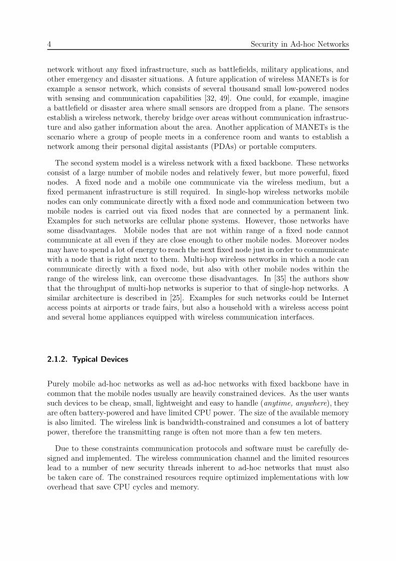
network without any fixed infrastructure, such as battlefields, military applications, andother emergency and disaster situations. A future application of wireless MANETs is forexample a sensor network, which consists of several thousand small low-powered nodeswith sensing and communication capabilities [32, 49]. One could, for example, imaginea battlefield or disaster area where small sensors are dropped from a plane. The sensorsestablish a wireless network, thereby bridge over areas without communication infrastruc-ture and also gather information about the area. Another application of MANETs is thescenario where a group of people meets in a conference room and wants to establish anetwork among their personal digital assistants (PDAs) or portable computers.
The second system model is a wireless network with a fixed backbone. These networksconsist of a large number of mobile nodes and relatively fewer, but more powerful, fixednodes. A fixed node and a mobile one communicate via the wireless medium, but afixed permanent infrastructure is still required. In single-hop wireless networks mobilenodes can only communicate directly with a fixed node and communication between twomobile nodes is carried out via fixed nodes that are connected by a permanent link.Examples for such networks are cellular phone systems. However, those networks havesome disadvantages. Mobile nodes that are not within range of a fixed node cannotcommunicate at all even if they are close enough to other mobile nodes. Moreover nodesmay have to spend a lot of energy to reach the next fixed node just in order to communicatewith a node that is right next to them. Multi-hop wireless networks in which a node cancommunicate directly with a fixed node, but also with other mobile nodes within therange of the wireless link, can overcome these disadvantages. In [35] the authors showthat the throughput of multi-hop networks is superior to that of single-hop networks. Asimilar architecture is described in [25]. Examples for such networks could be Internetaccess points at airports or trade fairs, but also a household with a wireless access pointand several home appliances equipped with wireless communication interfaces.
2.1.2. Typical Devices
Purely mobile ad-hoc networks as well as ad-hoc networks with fixed backbone have incommon that the mobile nodes usually are heavily constrained devices. As the user wantssuch devices to be cheap, small, lightweight and easy to handle (anytime, anywhere), theyare often battery-powered and have limited CPU power. The size of the available memoryis also limited. The wireless link is bandwidth-constrained and consumes a lot of batterypower, therefore the transmitting range is often not more than a few ten meters.
Due to these constraints communication protocols and software must be carefully de-signed and implemented. The wireless communication channel and the limited resourceslead to a number of new security threads inherent to ad-hoc networks that must alsobe taken care of. The constrained resources require optimized implementations with lowoverhead that save CPU cycles and memory.

2.2 Routing in Wireless Ad-hoc Networks 5
2.2. Routing in Wireless Ad-hoc Networks
As mentioned before, ad-hoc networks offer a number of new vulnerabilities of whichsome are caused by the different routing mechanisms employed in ad-hoc networks. Thespecial structure of these networks requires the routing mechanisms to be dynamic andon-demand. Routes have to be adapted to the constantly changing network topology.Moreover, routing is not only performed by special nodes, but by every member of thenetwork. Before we introduce the vulnerabilities of ad-hoc networks in the followingsection, let us briefly present two commonly used routing protocols for ad-hoc networks,namely DSR and AODV. This will allow the reader to better understand the cause ofsome of the vulnerabilities mentioned in the remainder of this chapter.
2.2.1. Dynamic Source Routing Protocol (DSR)
DSR [23] is an on-demand source routing protocol. It is referred to as ”on-demand”because route paths are discovered at the time a source sends a packet to a destinationfor which the source has no path.How is a route discovered? Suppose a node S wishes to communicate with a node Dbut does not know any path to D. It initiates a route discovery by sending a routerequest broadcast to its neighbors. This packet contains the destination address D. Theneighbors append their own address to the route request packet and rebroadcast it. Theprocess continues until the route request reaches D. D now sends back a route reply packetto S to inform it about the discovered route. D may choose the reverse path (all nodes onthe path the route request packet traveled have been appended to the packet) or initiatea new route discovery back to S. A source may receive multiple route replies from adestination, because there may be many routes from S to D. These routes are cached forfuture use.What happens if a link breaks? When two nodes are no longer within transmission range,the link is broken, and if an intermediate node detects such a link break when forwardinga packet to the next node on a path, it will send a message to the source that the link isbroken. The source then tries one of the cached alternative paths or if it does not haveany alternatives, it will initiate another route discovery [39].
2.2.2. Ad-hoc On-demand Distance Vector Routing Protocol (AODV)
The AODV [13] protocol is a table-driven routing protocol and it is based on the classicalBellman-Ford routing algorithm.How is a route discovered? When a source node S wants to send a packet to a destinationD and does not already have a route, it broadcasts a route request packet across thenetwork. Nodes that receive this packet update their information for the source node andtheir routing tables. If the node is either the destination S or knows a recent path to S, itmay send a route reply back to the source. Otherwise, the route request is rebroadcasted.

6 Security in Ad-hoc Networks
As the route reply propagates back to the source, the nodes on the way update theirrouting tables with the information about the route to D.Routes are maintained as long as data packets are traveling periodically from the sourceto the destination. Once the source stops sending packets, the link will time out andeventually be deleted from the routing tables of the intermediate nodes. If a link breakis detected by an intermediate node, a route error message is propagated back to S. If itstill desires the route, it has to reinitiate a route discovery [1].AODV typically minimizes the number of required broadcasts, i.e. nodes that are noton a selected path do not maintain routing information or participate in routing tableexchanges [14].
2.3. Security
Due to the dynamically changing topology and infrastructureless, decentralized character-istics, security is hard to achieve in mobile ad-hoc networks. Hence, security mechanismshave to be a built-in feature for all sorts of ad-hoc network based applications. In thissection, we talk about the security objectives for designing applications, possible attacksagainst ad-hoc networks and countermeasures that have already been proposed.
2.3.1. Security Goals
To secure a network, one usually considers the objectives availability, confidentiality,integrity, authentication and non-repudiation [45, 61, 68, 62]. In this subsection, we shortlyexplain the meaning of these terms.
Availability
Availability is a requirement that assures that systems work promptly and service is notdenied to authorized users. Attacks that affect availability are called denial of service(DoS) attacks. In an ad-hoc network, denial of service attacks could be launched atany layer. An adversary could employ jamming to interfere with communication on thephysical layer. On the network layer, an adversary could disrupt the routing protocoland disconnect the network. An adversary could also bring down high-level services. Bymassivly communicating with a node an attacker could prevent its victim from switchingto power save mode and thereby drain the victim’s battery.
Confidentiality
Confidentiality is the requirement that private or confidential information is not disclosedto unauthorized entities. The transmission of sensitive information, such as strategic or

2.3 Security 7
tactical military information, but also information about financial transactions, requiresconfidentiality. Not only the high-level information must remain confidential, but alsorouting information is not to be disclosed, as it might be valuable to identify and locatetargets in a battlefield or to create an information profile of a particular user.
Integrity
Integrity is the property that data has not been altered in an unauthorized manner whilebeing transferred. To assure integrity, unauthorized manipulation must be detectable.Due to the wireless communication interface a message in an ad-hoc network could becorrupted by benign failures, such impairment of radio propagation, or because of mali-cious attacks on the network. It is often not easy to distinguish between those two reasonsfor altered data, therefore many countermeasures that work for fixed infrastructure net-works (e.g. establishing a rating level for the trustworthiness of a node), cannot be easilyapplied to ad-hoc wireless networks.
Authentication
Authentication enables a node to ensure the identity of the peer node it is communicatingwith. When transmitting confidential data, it is important that the node that receivesthe information is the one it is meant for. A node could for example masquerade asanother node and gain unauthorized access to resources and sensitive information. Insome applications of ad-hoc networks, such as portable communication devices or sensornetworks for battlefield situations, the device could be tampered with, so it might not onlybe necessary to authenticate the device but also to make sure it has not been compromised.
Non-repudiation
Non-repudiation ensures that the originator of a message cannot deny having sent themessage. This goal is of particular importance in e-commerce applications or whenevercharging and billing is involved. Otherwise a user could for example order some productor service, possibly make use of it, and deny that she has ordered or received it whenthe provider wants to bill her. Non-repudiation is also useful for detecting compromisednodes. When a node A receives an erroneous message from a node B, non-repudiationallows A to accuse B using this message and thereby convince other nodes that B iscompromised.
2.3.2. Vulnerabilities of Ad-hoc Networks
Since there exists a broad range of applications for ad-hoc networks, the range of vulner-abilities is also quite broad. In this subsection, we present some of the most importantvulnerabilities, which are mentioned in [14], although they are not all relevant for ourparticular application.

8 Security in Ad-hoc Networks
Weak physical protection
In classical network applications, the physical protection of a node is often quite well.Servers or workstations are installed stationary in rooms that unauthorized persons cannotenter.In military applications, e.g. where soldiers are carrying mobile devices while fightingon a battlefield or where small sensors are dropped from a plane, one can easily imaginethat mobile nodes are subject to capturing, compromising and hijacking. In such hostileenvironments it is almost impossible to provide perfect physical protection.Today, portable devices like mobile phones or PDAs are getting smaller and smaller. Sucha small device can be easily lost or stolen and misused by an adversary. Hence, we alsohave to pay attention to this problem in civilian applications.As a consequence the case of compromised devices should always be considered duringthe design of an ad-hoc network system.
Constrained capabilities
As mentioned before, devices in ad-hoc networks have constrained capabilities concerningCPU power, battery power and transmission bandwidth. These limited resources aresubject to denial of service attacks.Denial of service attacks against CPU power and transmission bandwidth are well knownfrom classical networks. One or more adversaries flood a node with so many requests ata time that the node cannot process them any more. As a result, benign users cannot beserved either.In [60] Stajano and Anderson present a denial of service attack that makes use of thelimited battery power of ad-hoc networking devices. They call the attack sleep deprivationtorture. Most portable devices try to spend as much time as possible in sleep mode inorder to minimize energy consumption. In fact, the radio device and the CPU consume themost power in modern devices, so they are turned on only once a while during sleep mode.An attacker might communicate with a particular node in a legitimate way just to keep itfrom going into sleep mode. The adversary thereby exhausts the victim’s batteries muchfaster than usual. Finally, when it has run out of battery power, the victim is disabled.So, this attack is more powerful than DoS attacks against CPU power or transmissionbandwidth, because the device is not only disabled for the time of the attack, but forever(at least until the next battery change or recharge).
Required cooperative participation
The first applications that have been proposed for ad-hoc networks take place in militaryor disastrous situations. In those cases all nodes usually belong to one authority andhave a common goal. However, in civilian applications one can no longer assume thatthe nodes have a common goal. Moreover, users may act selfish and are not concerned

2.3 Security 9
about overall network performance. Therefore, recent research deals with the preventionof non-cooperative behavior.First of all, why is cooperation so important in multi-hop ad-hoc networks? To transmita message to a node B across the network, the originating node A often has to route itvia intermediate nodes, because the receiving node B is not within the transmission rangeof A’s wireless interface. Hence, to keep the network functioning, the intermediate nodeshave to spend energy, CPU power and transmission bandwidth to forward other node’smessages. But as mentioned before, energy, CPU power and transmission bandwidth arelimited resources for most devices in an ad-hoc network, so there is a trade-off betweencooperation and survival. At the same time, if a node does not forward foreign messages,other nodes might not forward either and thereby deny service [10].
Weaknesses of the wireless medium
It is part of the nature of the wireless medium, that it is not an exclusive use medium. Asa consequence, possible attacks range from passive eavesdropping to active impersonation,message replay and message distortion. Actively interfering attacks allow the adversaryto delete messages, to inject erroneous messages, to modify messages and to impersonateas a node [68].
Attacks on the network layer
Due to the dynamically changing topology of ad-hoc networks (i.e. nodes join and leave,disconnect temporarily and move around), routing has to be organized in a dynamic way.This opens among others the following security vulnerabilities, which are mentioned, forexample, in [10, 14, 21].
1. Incorrect forwarding: As mentioned in the section about cooperation, a nodecould, instead of following the routing protocol, deny forwarding packets. Thiscould also be done in a selective way, i.e. forward only a set of packets, maybe for aparticular group of nodes. Furthermore a node could modify other nodes’ answersto route requests and influence the routing throughout the network.
2. Traffic deviation: A malicious node could falsely advertise very attractive routes(for example, claim that the destination is only one hop away) and thereby convinceother nodes to route their messages via that malicious node. An attacker could usethis to collect information, influence network routes, and prevent some packets frombeing transmitted.
3. Flooding with route updates: By sending route updates at short intervals anadversary could overload the network. This is another kind of denial of serviceattack.

10 Security in Ad-hoc Networks
4. Black hole attack: This is a combination of traffic deviation and incorrect for-warding. A node advertises falsely itself as having the shortest path to the nodewhose packet it wants to intercept. Now many nodes route their packets to thatdestination via the malicious node, because it seems to be the most efficient route.The adversary now simply drops these packets.
5. Gray hole attack: In this special case of the black hole attack, the attackerselectively drops some packets but not others. The adversary may, for example,forward routing packets but not data packets. Alternatively, she may only forwardpackets for certain destinations or from particular origins.
6. Wormhole attack: In [21], the authors introduce a new attack that involves apair of attackers that are linked via a private network connection. These maliciousnodes tunnel packets they receive from the network through their direct link andrebroadcast them at the other end of the wormhole. This potentially disrupts routingby short-circuiting the normal flow of routing packets and offers the possibility tocontrol a considerable amount of traffic.
2.3.3. Approaches to Establish Security in Ad-hoc Networks
Let us now present some approaches that have been proposed to counteract the securitythreads of ad-hoc networks. There exists a broad range of problems from authenticationand key distribution, over secure routing, detection of misbehavior to motivating coop-erative behavior. In the following, we give some examples for approaches to tackle theseproblems.
Authentication and key distribution
� Resurrecting duckling: In [60] Stajano and Anderson present a mechanism toauthenticate users by imprinting. Analogous to a duckling that recognizes the firstmoving subject it sees as its mother, the node accepts a symmetric encryption keyfrom the first device that sends such a key on a secure channel, e.g. by physi-cal contact during the device initialization. The node may be imprinted severaltimes. After performing this kind of key exchange, an encrypted connection can beestablished.
� Self-organized public key certificates: Public-key certificates issued, storedand distributed by the users are part of a model proposed by Hubaux, Buttyanand Capcun [22]. In this model, each node keeps a small part of the certificationknowledge. By sharing this information, several certificate paths can be found.
� Localized certification services: Kong, Zerfos, Luo, Lu and Zhang [29] suggesta public key infrastructure with certification authorities based on threshold secretsharing. The secret shares are updated periodically. For providing certificationservices K one-hop neighbors are needed within a given time window.

2.3 Security 11
� Asynchronous threshold security: Zhou and Haas [68] propose a key manage-ment service based on threshold cryptography to distribute trust among a set ofspecial nodes. Cryptographic operations can only be performed jointly by t + 1nodes, but are infeasible for t or less nodes, even by collusion. Furthermore, theauthors take advantage of inherent redundancies in ad-hoc networks due to mul-tiple routes to enable diversity coding. The basic idea is to transmit redundantinformation through additional routes for error detection and correction. TherebyByzantine failures given by several corrupted nodes or collusions can be tolerated.
Secure routing
� Secure Routing Protocol: Only assuming a security association between end-points, Papadimitratos and Haas propose a routing protocol [50] that guaranteesa correct route discovery without the need of trusted intermediate nodes. Routerequests reach the destination along with a unique random query identifier. Theroute request reply contains a message authentication code computed over the path.The protocol is constructed such that compromised or replayed route requests willnever reach the source.
� ARIADNE: This secure on-demand routing protocol by Hu, Perrig, and Johnson[21] prevents compromised nodes from disturbing uncompromised routes, i.e. routesthat consist of uncompromised nodes. It uses a key management protocol based onone-way key chains called TESLA, which relies on loosely synchronized clocks. Theprotocol is based on DSR (Section 2.2) and protects the routes with hash chainsand message authentication codes.
� SAODV: In [66], a security extension for AODV (Section 2.2) has been proposedby Zapata. Its basic idea is that the source appends a digital signature and a keyedhash chain on the control messages for route discovery. As the message traversesthe network, the intermediate nodes verify the signature and update the hash chain.Thereby integrity, authentication and non-repudiation for source and destination areprovided.
Detection of attackers
� Intrusion detection: To suite the needs of wireless ad-hoc networks Zhang andLee [67] postulate that intrusion detection and response systems should be bothdistributed and cooperative. With statistical anomaly detection on several networklayers every node watches for intrusions and a majority voting mechanism is usedto classify behavior by consensus. Possible responses to compromised nodes arere-authentication or isolation.
� Watchdog and pathrater: For DSR, Marti, Giuli, Lai and Baker [39] introduce awatchdog that detects denied packet forwarding and a pathrater that manages trust

12 Security in Ad-hoc Networks
and routing policies. Misbehavior such as packet dropping is detected by utilizingthe promiscuous mode of the wireless interface, i.e. the ability of nodes to overheartheir neighbors’ communication. Successfully detected malicious nodes are avoidedin future routes, however, their outgoing data packets are still forwarded to thedestinations.
� CONFIDANT: This acronym stands for ’Cooperation Of Nodes, Fairness In Dy-namic Ad-hoc NeTworks’ and has been proposed by Buchegger and Boudec [8, 9, 10].This scheme detects malicious nodes by means of observation or reports about sev-eral types of attacks. Nodes have a monitor for observations, reputation recordsfor first-hand and trusted second-hand observations, trust records to control trustgiven to received warnings, and a path manager for nodes to adapt their behavioraccording to reputation. Malicious nodes that have been detected are isolated fromthe network.
Motivating cooperation
� Nuglets or Counters: As incentives for cooperation Buttyan and Hubaux [11]propose so-called nuglets that serve as a per-hop payment in every packet or counters[12] to encourage forwarding. Both nuglets and counters reside in a secure modulein each node, are incremented when nodes forward for others and decremented whenthey send packets for themselves.
� Secure Charging Protocol: Lamparter, Paul, and Westhoff [30] propose a proto-col that motivates intermediate nodes to forward packets by giving them a monetaryreward. At the same time, nodes are charged for sending or receiving data. Theenvisioned ad-hoc network is not purely mobile, but it is an access network withsome fixed backbone that provides for example Internet or intranet access. Theprotocol uses digital signatures and keyed hash chains. The certificate authority ismaintained by a network service provider that also manages charging and rewarding.

Digital Signatures 13
3. Digital Signatures
One part of this work is the cryptographic analysis of the secure charging protocol. Webriefly mentioned in the last chapter, that it employs digital signatures. For this reason,let us provide some information about the most common digital signature schemes beforestarting the actual analysis.
The concept of a digital signature was introduced in 1976 by Diffie and Hellman [15, 16].Digital Signatures have been designed in order to provide the digital counterpart to ahandwritten signature. Basically, a digital signature is a number that depends on somesecret only known to the signer (the signer’s secret key) and the content of the message tobe signed. The design goal is to make the signature verifiable, i.e. an unbiased third partyshould be able to check, without knowing the secret of the signer, whether the messagehas been indeed signed by a particular person. Such a verification may be necessary wheneither the signer denies having signed the message (repudiation) or when an adversaryhas faked a signature and claims that it is valid.
Figure 3.0.1 Illustration of digital signatures.
This is Alice‘smessage
9001 5098 3cd2 4fb0d696 3f7d 28e1 7f72
Hash-Function
0cc1 75b9 c0f1 b6a831c3 99e2 6977 2661
Encryption
Alice‘sPrivate Key
This is Alice‘sMessage
0cc1 75b9 c0f1 b6a831c3 99e2 6977 2661 Alice‘s
Public Key
This is Alice‘smessage
9001 5098 3cd2 4fb0d696 3f7d 28e1 7f72
Hash-Function
9001 5098 3cd2 4fb0d696 3f7d 28e1 7f72
0cc1 75b9 c0f1 b6a831c3 99e2 6977 2661
Decryption
= ?
Alice Bob
Most digital signature schemes work as illustrated in Figure 3.0.1. Suppose Alice wantsto send Bob a digitally signed message. For the sake of simplicity, let us assume thatBob already owns a copy of Alice’s public key and Alice owns the corresponding private(secret) key. Moreover, we assume that Bob is sure that the key he owns is the public keyof Alice and not of somebody else.In the first step of the signature scheme, Alice calculates a hash value of her message using

14 Digital Signatures
some one-way hash function and converts it to an integer. A one-way hash function mapsa message of arbitrary size to a bit string of predefined length. An important propertyof such a hash function is that it is collision resistant, i.e. it is computationally infeasi-ble to find two distinct inputs that hash to the same output. In the following step, thehash value is used together with Alice’s private key as input value for some mathematicalfunction. This step is called ’Encryption’ in Figure 3.0.1.Now, Alice appends the output of this mathematical function, which is the digital signa-ture of the original message, to her message and sends both to Bob.Bob extracts the digital signature part from the received message and uses it as inputargument of some other mathematical function. Together with Alice’s public key as asecond input argument, Bob calculates an integer that should be equal to the value thatAlice used as input for her encryption function. This step is called ’Decryption’ in thefigure.Bob uses the hash function on the message he received from Alice to calculate a hashvalue. By comparing this hash value to the output of his decryption function, he candetect whether the message has been altered.If both values are equal, he knows that it has not been altered. Moreover, if Bob knowsfor sure that the public key he used to verify the message belongs to Alice, he can alsobe sure that Alice and not somebody else has sent the message, since only she owns thecorresponding private key.
In the following, we introduce the RSA, DSA and ECDSA signature schemes and discusstheir underlying mathematical problems and possible attacks.
3.1. The RSA Signature Scheme
The RSA signature scheme was discovered by Rivest, Shamir, and Adleman [51]. Itwas the first practical signature scheme based on public-key techniques. The underlyingcomputationally hard mathematical problem for the RSA signature scheme is the integerfactorization problem (IFP)[41]:
Given a composite number n that is the product of two large prime numbersp and q, find p and q.
Since it is part of the public key, an adversary has access to the modulus n. Once pand q are computed, the system is broken and the attacker can use Algorithm 3.1.1 todetermine the secret key.
Algorithm 3.1.1 summarizes how a key pair, i.e. a public and the corresponding privatekey, for the RSA signature scheme can be generated. The steps for signing a message aregiven in Algorithm 3.1.2 and the steps for verifying a message can be found in Algorithm3.1.3.

3.1 The RSA Signature Scheme 15
Algorithm 3.1.1 Key generation for the RSA signature scheme [45]
OUTPUT: The public key (n, e) and the private key d.
1: Generate two large distinct random primes p and q, each roughly the same size.2: Compute n = pq and φ = (p− 1)(q − 1).3: Use the extended Euclidean algorithm to compute the unique integer d, 1 < d < φ,
such that ed ≡ 1 (mod φ).4: The public key is (n, e); the private key is d.
Algorithm 3.1.2 RSA signature generation [45]
INPUT: The message m, the public key (n, e), and the private key d.OUTPUT: The digital signature s.
1: Compute the hash value of the message m = h(m), an integer in the range [0, n− 1].2: Compute s = md mod n.3: The signature for m is s.
Algorithm 3.1.3 RSA signature verification [45]
INPUT: The message m, the public key (n, e) of the signer and the signature s onm.
1: Compute m = se mod n.2: Verify that m = h(m); if not, reject the signature.
In [41] the following attacks for the IFP are mentioned:
� Continued Fraction Algorithm: This algorithm is based on the idea of usinga factor base of primes and generating an associated set of linear equations whosesolution leads to a factorization. It could factor numbers of up to 133-bits.
� Quadratic Sieve Algorithm (QS): This algorithm is based on the same idea asthe continued fraction algorithm and can be easily parallelized to permit factoringon distributed networks.
� General Number Field Sieve (NFS): Also based on the idea of the continuedfraction algorithm, the NFS is supposed to be the fastest known algorithm forfactoring integers having at least 400 bits.
� Elliptic Curve Factoring Method (ECM): This algorithm attempts to exploitspecial features of an integer to be factorized. It tends to find small factors first.

16 Digital Signatures
3.2. The Digital Signature Algorithm (DSA)
The Digital Signature Algorithm has been proposed in August of 1991 by the U.S. NationalInstitute of Standards and Technology (NIST). The underlying computationally hardmathematical problem is the discrete logarithm problem (DLP)[41]:
Given a prime p, a generator α of Zp, and a non-zero element β ∈ Zp, find theunique integer l, 0 ≤ l ≤ p− 2, such that β ≡ αl (mod p).
The integer l is called the discrete logarithm of β to the base α. If p is a prime number,then Zp is a finite field denoted by the set of integers {0, 1, 2, . . . , p− 1}, where additionand multiplication are performed modulo p. There exists a non-zero element α ∈ Zp suchthat each non-zero element in Zp can be written as a power of α; such an element α iscalled a generator of Zp.
Algorithm 3.2.1 summarizes how a key pair, i.e. a public and the corresponding privatekey, for the DSA signature scheme can be generated. The steps for signing a message aregiven in Algorithm 3.2.2 and the steps for verifying a message can be found in Algorithm3.2.3.
Algorithm 3.2.1 Key generation for the DSA [45, 24]
OUTPUT: The public key (p, q, α, y) and the private key a.
1: Select a 160-bit prime q and a 1024-bit prime p with the property that q|p− 1.2: Select a generator α of the unique cyclic group of order q in Z
∗p, i.e. select an element
g ∈ Z∗p, compute α = g(p−1)/q mod p, and repeat this if α = 1.
3: Select a random integer a such that 1 ≤ a ≤ q − 1.4: Compute y = αa mod p.5: The public key is (p, q, α, y); the private key is a.
Algorithm 3.2.2 DSA signature generation [45]
INPUT: The message m, the public key (p, q, α, y), and the private key a.OUTPUT: The digital signature (r, s).
1: Select a random integer k, 0 < k < q.2: Compute r = (ak mod p) mod q.3: Compute k−1 mod q.4: Compute s = k−1{h(m) + ar} mod q, where h(m) is the hash value of the message
m.5: The signature for m is (r, s).

3.3 The Elliptic Curve Digital Signature Algorithm (ECDSA) 17
Algorithm 3.2.3 DSA signature verification [45]
INPUT: The message m, the public key (p, q, α, y) of the signer and the signature (r, s)on m.
1: Verify that 0 < r < q and 0 < s < q; if not, reject the signature.2: Compute w = s−1 mod q and the hash value h(m).3: Compute u1 = w · h(m) mod q and u2 = rw mod q.4: Compute v = (αu1yu2 mod p) mod q.5: Accept the signature if and only if v = r.
According to [41], there exist the following known attacks against DSA and the discretelogarithm problem:
� Index Calculus Method: The fastest general-purpose algorithms known for solv-ing the DLP are based on the index calculus method. In this method, a databaseof small primes and their corresponding logarithms is constructed. Subsequently,logarithms of arbitrary field elements can be easily obtained. This is reminiscent ofthe factor base methods for integer factorization. If an improvement in the algo-rithms for either the IFP or DLP is found, then shortly after this a similar improvedalgorithm can be expected to be found for the other problem. The index calculusmethod can be easily parallelized.
� Number Field Sieve Algorithm: This is the best current algorithm known forthe DLP and has precisely the same asymptotic running time as the correspondingalgorithm for factoring integers.
3.3. The Elliptic Curve Digital Signature Algorithm (ECDSA)
A variant of DSA based on elliptic curves is ECDSA. It was first proposed in 1992 byScott Vanstone [63]. The underlying computationally hard mathematical problem is theElliptic Curve Discrete Logarithm Problem (ECDLP)[41]:
Given an elliptic curve E defined over Fq, a point P ∈ E(Fq) of order n, anda point Q ∈ E(Fq), determine the integer l, 0 ≤ l ≤ n− 1, such that Q = lP ,provided that such an integer exists.
This discrete logarithm problem over elliptic curves is considered to be significantly harderthan the DLP over Zp, which is the mathematical basis for DSA. Therefore, the strength-per-key-bit is substantially higher than in DSA and, hence, smaller parameters (keys) canbe used for elliptic curve cryptosystems to achieve equivalent levels of security.

18 Digital Signatures
In order to facilitate interoperability, the domain parameters for ECDSA, which arethe parameters of the curve E, the underlying finite field Fq and a base point G ∈ E(Fq),have to be negotiated and agreed upon by the communication partners. The curve isusually determined by its two parameters a and b and the curve equation. For the finitefield F2m , the curve equation is given by the equation
y2 + xy = x3 + ax2 + b, (3.1)
which is the same for all m. The base point G is defined by its affine coordinates xG andyG. Usually, the order n of the point G is also part of the domain parameters.
Algorithm 3.3.1 summarizes how a key pair, i.e. a public and the corresponding privatekey, for the ECDSA signature scheme can be generated. The steps for signing a messageare given in Algorithm 3.3.2 and the steps for verifying a message can be found in Algo-rithm 3.3.3. Signature generation and verification requires the computation of the hashvalue of the message using the Secure Hash Algorithm (SHA-1) [45], which was proposedby the U.S. National Institute for Standards and Technology (NIST).
Algorithm 3.3.1 Key generation for the ECDSA [24]
INPUT: The elliptic curve domain parameters.OUTPUT: The public key Q and the private key d.
1: Select a random integer d in the interval [1, n− 1].2: Compute Q = dG.3: The public key is Q and the private key is d.
Algorithm 3.3.2 ECDSA signature generation [24]
INPUT: The message m, the elliptic curve domain parameters, the public key Q, andthe private key d.OUTPUT: The digital signature (r, s).
1: Select a random integer k, 0 < k < n.2: Compute kG = (x1, y1) and convert x1 to an integer.3: Compute r = x1 mod n. If r = 0 then go to Step 1.4: Compute k−1 mod n.5: Compute SHA-1(m) and convert this bit string to an integer e.6: Compute s = k−1(e + dr) mod n. If s = 0 then go to Step 1.7: The signature for the message m is (r, s).

3.4 Performance Comparison of RSA, DSA and ECDSA 19
Algorithm 3.3.3 ECDSA signature verification [24]
INPUT: The elliptic curve domain parameters, the message m, the public key Q of thesigner and the signature (r, s).
1: Verify that r and s are integers in the interval [1, n− 1]2: Compute SHA-1(m) and convert this bit string to an integer e.3: Compute w = s−1 mod n.4: Compute u1 = ew mod n and u2 = rw mod n.5: Compute X = u1G + u2Q.6: If X = O, then reject the signature. Otherwise, convert the x-coordinate of X to an
integer x1, and compute v = x1 mod n.7: Accept the signature if and only if v = r.
A discussion about possible attacks on elliptic curve cryptosystems and their level ofsecurity can be found in Section 5.5.
3.4. Performance Comparison of RSA, DSA and ECDSA
Before comparing the performance of different signature schemes, i.e. the execution timesof the signature generation and signature verification, we have to agree which key sizesprovide a comparable level of security. This is necessary, because the computationalhardness of the underlying mathematical problems is different and some schemes needsmaller key sizes than others for achieving the same level of security.
In a Standards for Efficient Cryptography document [44] a list of elliptic curves withdifferent key sizes is given. The list also contains RSA / DSA key sizes that achievecomparable levels of security. Table 3.4.1 contains these values.
Clearly, the key sizes for elliptic curves are significantly smaller than those for RSA /DSA. Additionally, the key size does not increase as fast as the one of RSA / DSA. Figure3.4.1 gives a good impression of this behavior. Hence, ECDSA has a major advantage fordesigns that might need an increased level of security in the future.
Lenstra and Verheul present in their paper [33] a recommendation of key sizes for sym-metric cryptosystems, RSA, and discrete logarithm based cryptosystems both over finitefields and over groups of elliptic curves over prime fields. The authors formulate a modelthat based on Moore’s law incorporates future changes of the available computationalpower and the arising hardware costs. Their model also takes into account future progressin cryptanalysis. Based on some hypotheses, e.g. that DES has been secure enough forcommercial applications until 1982, the authors come up with an equation that predictsthe computational load they consider to be infeasible until year y. The authors combinetheir model with data points that evaluate the computational power necessary to break

20 Digital Signatures
certain cryptosystems with certain key sizes. Finally, Lenstra and Verheul present a tablestating for each year until 2050 which minimum key size for which cryptosystem can beconsidered to be secure until that year.
Figure 3.4.1 Size of the ECDSA key compared to the size of the RSA / DSA keyproviding a similar level of security
100
150
200
250
300
350
400
450
1000 2000 3000 4000 5000 6000 7000 8000
Siz
e of
EC
DS
A k
ey [b
its]
Size of RSA key [bits]
Lenstra and Verheul tend to recommend key sizes for elliptic curve cryptosystems thatare smaller than those in the standard document cited above. As it is dated before thestandard document and as the authors do not directly compare elliptic curve cryptosys-tems over binary fields, we prefer to use Table 3.4.1 as basis.
In a whitepaper [40] from 1997, Certicom Corp. examines RSA and elliptic curve basedcryptosystems with respect to their security and efficiency. They point out that the bestknown general-purpose algorithm for breaking RSA has a sub-exponential time complex-ity whereas solving the elliptic curve discrete logarithm problem with the best generalalgorithm has fully exponential time complexity. For increasing levels of security, thegap between ECC key sizes and RSA key sizes dramatically increases. In terms of effi-ciency, Certicom claims that ECC outperforms RSA with respect to computational over-head, storage requirements, and bandwidth requirements. Their benchmarks are basedon 160-bit ECC and 1024-bit RSA. To their opinion implementations of elliptic curvecryptosystems that are roughly 10 times faster than RSA can be realized. However, theyalso concede that a short public exponent in RSA may lead to signature verification timesthat are comparable with ECC.

3.4 Performance Comparison of RSA, DSA and ECDSA 21
Table 3.4.1 SECG recommended elliptic curves over F2m [44]
Curve Name Curve Type Key Size equiv. RSA / DSA Key Size
sect113r1sect113r2
random 113 512
sect131r1sect131r2
random 131 704
sect163k1 Koblitz 163 1024sect163r1sect163r2
random 163 1024
sect193r1sect193r2
random 193 1536
sect233k1 Koblitz 233 2240sect233r1 random 233 2240
sect239k1 Koblitz 239 2304
sect283k1 Koblitz 283 3456sect283r1 random 283 3456
In an RSA Laboratories Technical Note [52] from 1997, Robshaw and Yin analyze cryp-tosystems based on RSA and on ECDSA. For ECDSA with a key size of 160 bits and1024-bit RSA, which they found to achieve a comparable level of security, the authorscompare the performance of both schemes in terms of storage requirements and computa-tional speed. While its short key size leads to clear advantages for ECDSA with respectto storage requirements, their findings for the computational speed do not allow such aclear statement. According to their benchmarks, the RSA sign operation is about 7 timesslower than the one of ECDSA, but the verify operation is more than 6 times faster. Rob-shaw and Yin fear that elliptic curve cryptography might still offer some yet undiscoveredloopholes due to the complex mathematical theory behind it.
Another article [65] by Wiener published in RSA Laboratories’ CryptoByte newslettercontains a comparison between 1024-bit RSA, 1024-bit DSA and 168-bit ECDSA. Theverification times of RSA are found to be more than 30 times faster than those of ECDSA.The signature generation is measured to be around 8 times slower (see Table 3.4.2 forthe exact results). The author points out that the optimal choice of a signature schemedepends on the particular application. Discussing several different applications for public-key cryptosystems, he comes to the conclusion that RSA is well suited, for example,for certificate-based systems that require only few signature generations but thousandsof signature verifications. However, in wireless communication scenarios Wiener favorsECDSA as public-key algorithm, because the short key size and low signature overheadsave transmission bandwidth and lead to smaller silicon implementations.

22 Digital Signatures
Table 3.4.2 Digital signature timings (milliseconds on a 200 MHz Pentium Pro) [65].
RSA-1024 DSA-1024 ECDSA-168(e = 3) (over F168)
Sign 43 7 5Verify 0.6 27 19Key generation 1100 7 7
An evaluation of the performance of ECC in protocol applications can be found in [18].Besides adding ECDSA support to OpenSSL (see also Section 7), the authors analyze theperformance influence of ECDSA and RSA on the SSL protocol. Their measures are theHandshake Crypto Latency , which is essentially the sum of the times the client and theserver spend doing public key operations, and the Server Crypto Throughput , which is therate at which the server can perform the cryptographic operations. For a security levelof 1024-bit RSA, ECC performed more than five times better in terms of Server CryptoThroughput. However, in terms of Handshake Crypto Latency, the performance dependson the underlying scenario. For a PDA talking to a server, RSA beats ECC, while forPDA talking to PDA or server talking to server, ECC is nearly twice as fast as RSA. Inexperiments with a security level of 2048-bit RSA, ECC always outperformed RSA. Forthis reason, the authors see a performance advantage for ECC at higher levels of security.
Obviously, the opinions about which digital signature scheme is the best are not clear.However, most sources agree that RSA would be a good choice for systems in which sig-nature verification dominates execution times and ECDSA for systems in which signaturegeneration dominates execution times.

The Secure Charging Protocol (SCP) 23
4. The Secure Charging Protocol (SCP)
Let us now take a more detailed look at one particular approach to enhance security inad-hoc networks. In [30], Lamparter, Paul, and Westhoff proposed a protocol for chargingsupport in multi-hop ad-hoc networks. The so-called Secure Charging Protocol employsdigital signatures as cryptographic tool to establish authentication, integrity, and non-repudiation of charging information.
In this chapter, we point out the benefits of this protocol and describe the protocolarchitecture. Afterwards, we analyze the protocol from a cryptanalytic point of view andassess the required level of security as well as different digital signature schemes.
4.1. Underlying Scenario
First, let us summarize the scenario Lamparter et al. envisioned for their proposal:
The ad-hoc network is not purely mobile, but it is an access network with some fixedbackbone that provides for example Internet or intranet access (see also Section 2.1.1).An access point (AP) forms the gateway between both networks. When a mobile node(MN ) wants to communicate with a corresponding node (CN ) in the fixed network, theAP may or may not be within transmission range. If it is not within range, the MN mayuse intermediate nodes (Ni) in a hop-by-hop fashion to reach the access point. When thecorresponding node is within the ad-hoc network, AP can be bypassed and the CN canbe reached in multi-hop mode.
The proposed protocol does not handle colluding attacks, i.e. any attack for which themobile node MN or corresponding node CN and one or more intermediate nodes have tocooperate shall not be prevented.
4.2. Benefits
The concept of multi-hop ad-hoc networks offers several advantages over single-hop net-works. Nevertheless, there are also some problems to be solved before such networkscan be deployed. The protocol proposed by Lamparter, Paul, and Westhoff tackles thefollowing two difficulties.
On first sight, a network service provider (NSP) is not interested in deploying multi-hop networks, because commonly users pay the NSP for providing the communication

24 The Secure Charging Protocol (SCP)
infrastructure. However, in a multi-hop network, users may communicate directly witheach other without using any infrastructure provided by the NSP. Obviously, the amountof traffic that is transmitted via the infrastructure of the NSP is less in a multi-hopnetwork than in a single-hop network. Consequently, the main source of income of theNSP is endangered by such network structures.
On the other hand, why should a node forward other nodes’ data packets? Mobiledevices have only limited battery power and they usually try to spend as much time aspossible in sleep mode in order to save energy. However, whenever the device has to com-municate via its wireless interface, the power consumption rises dramatically. Forwardingforeign traffic would obviously reduce the time such a device can spend in sleep mode,simply because it has to transmit more data.
Lamparter, Paul, and Westhoff come up with an idea that solves both problems. Theysuggest charging the nodes for any transmitted or received data packet, regardless whetherit is transmitted with or without using the infrastructure of the NSP. On the other hand,the nodes that forward foreign traffic are given a monetary reward. If the ratio betweenthe charged and the rewarded amount of money is properly balanced, the NSP is able toearn money even if its infrastructure is not used. In this case, the users pay the NSP forproviding certificate authority, network administration services and a reliably functioningad-hoc network. Thereby, the NSP is more likely to deploy such a network, becausethe reduced number of necessary access points reduces spendings and billing of the usersincreases income. At the same time, users are encouraged to participate in forwarding,since this reduces their cost for transmitting information – of course with the disadvantageof increased power consumption.
Motivating users to cooperate and share resources as Lamparter, Paul, and Westhoffsuggest is a striking approach to prevent dishonest passive behavior. This reduces theneed to detect and sanction non-cooperating nodes and allows detection schemes to focuson the few actively malicious nodes.
4.3. Description
In the following, we present a shortened version of the description of the secure chargingprotocol architecture as it is provided by the authors of [30]. Their paper contains furtherdetails, in particular about authentication, charging and pricing.
When the MN joins the access network it first authenticates with the NSP. The MNprovides its credentials to the NSP, the NSP verifies the home domain of MN, and sendsback authorization information to MN.
At the source node MN :
1. Path finding : The MN uses some on-demand source routing protocol (see also Sec-tion 2.2) to find the path MN, N1, N2, . . . , Nn, CN.

4.3 Description 25
2. Providing MN’s legal registration: MN sends the following security information alongwith the data:
a) To secure originator, destination and hops: MN ’s digital signature on the routeMN, N1, N2, . . . , Nn, CN,
b) To initialize a hash chain: A keyed hash value on MN and CN,
c) To reveal key information: An identity certificate of MN to prove registrationto intermediate nodes.
At each intermediate node Ni:
1. Service provision: Ni checks the signature of MN. In case of a correct signature, Ni
can be sure that an authorized MN is willing to communicate.
2. Hash chain update: Ni computes the next value of the hash chain, i.e. the keyedhash value of the received hash value using Ni’s key.
3. Packet forwarding : Ni forwards the packet to the next node on the route.
At the last intermediate node Nn (in addition to the previously mentioned usual procedureat intermediate nodes):
1. Service provision confirmation: Nn acquires step-by-step a non-repudiative messagefrom CN, confirming the received amount of data.
2. Notification of AP : Nn (later on) notifies the AP about the involved forwardingnodes and the service provision confirmation.
At the destination node CN :
The destination node CN signs the amount of data received from Nn.
At the access point AP :
Service provision verification: When it receives the hash chain and the service provisionconfirmation, the AP verifies the participation of each node and books the reward/costto the accounts of the participating nodes.

26 The Secure Charging Protocol (SCP)
Figure 4.3.1 Network scenario for the Secure Charging Protocol
AP
MN CNI1
In
4.4. Analysis of the Cryptographic Requirements
In their paper, Lamparter, Paul, and Westhoff proposed several cryptographic primitivesfor their protocol. In this section, we have a closer look at the cryptographic requirementsof the protocol. The main design goals for the protocol are motivated by the constrainedcapabilities of the target platform. In general, cryptographic operations are said to berather expensive with respect to execution time, which is in particular problematic dueto the constrained CPU power of a portable device. Therefore, one goal is to choosecryptographic primitives that require only a small amount of CPU power. Another goalis certainly to choose primitives that keep the protocol overhead as small as possible,because the bandwidth of the wireless communication channel is also quite limited.
The cryptographic primitives proposed by Lamparter, Paul, and Westhoff in [30] forthe secure charging protocol are
� unkeyed hash SHA-1,
� keyed hash MD5-MAC,
� digital signatures based on elliptic curves (ECDSA).
The hash functions turn out to be rather cheap with respect to CPU time compared to thedigital signature operations. According to the OpenSSL speed program the computationof MD5-MAC requires approximately 250 nanoseconds and the RSA verify operationtakes more than 10 milliseconds on an Intel Pentium II Workstation at 300MHz (factor4 ·104). Therefore we will only consider different digital signature schemes in the followingargumentation and neglect the influence of the hash functions.

4.4 Analysis of the Cryptographic Requirements 27
4.4.1. Required Level of Security (Key Size)
A typical application scenario for the secure charging protocol is the provision of wirelessInternet access at an airport terminal or railway station. These places have in commonthat the usual user does not stay longer than several hours at that place. Consequently,most user certificates and with them private keys and public keys need only to be validfor a short time, e.g. 24 hours. In case of longer stays, one could simply perform a keyexchange every 24 hours and provide fresh certificates.
The objective of someone who attacks the secure charging protocol is certainly to getuncharged network access or to only collect the rewards without paying. However, theamount of money involved can be expected to be rather low. Today’s (March 2003) pricesfor wireless network access range from 3.75
�per hour at the Munich airport [4] to 9
�
per hour at the CeBIT fair [20]. Thus, the financial harm of successfully breaking onepair of keys is less than 200
�. Consequently, one can expect that an attacker will not
spend a large amount of money to break a key. Note, that breaking a key of the securecharging protocol can only be used to compromise the node to which the key belongs.No secret information will be revealed; the attacker may forge only the secure chargingprotocol signatures of the compromised node.
Using the results of the DES Challenge III [53] as a basis, we can determine the keysize for our purposes according to the recommendations of Lenstra and Verheul [33]. Inthe DES Challenge III launched in January 1999 by RSA Data Security, Inc., a messageencrypted with the 56-bit DES algorithm has been broken within 22 hours and 15 minutes.As explained above, keys that can be broken in approximately this amount of time stillprovide enough security for our purposes. In their paper, Lenstra and Verheul offerequations to adapt their recommendations to this level of security. Table 4.4.1 containsthese modified recommendations.
Table 4.4.1 Lower bound for RSA key sizes assuming that DES can be trusted until 1998(as recommended by Lenstra and Verheul in [33]).
Year RSA Key Size
2003 7442005 8102010 9902015 11912020 14162025 16642030 1937
However, we feel that these recommendations are too careful. So far, the largest RSAChallenge Number that has been factored in RSA Security’s Factoring Challenge [43] is

28 The Secure Charging Protocol (SCP)
a 512-bit number. The factoring was finished in August 1999, took 3.7 months and theCPU-effort is estimated to approximately 8000 MIPS years. We feel that this marginof security would still be sufficient for our particular application. Lenstra and Verheulrecommend a minimum key size of 513 bits for RSA in the year 1986, so we obtainedthe values in Table 4.4.2 by taking their recommendations for the year 1986 + x as guidevalue for our implementation in the year 1999 + x. To our opinion this is still a correctinterpretation of their recommendations, simply with a different margin of security. Note,that we do not claim that breaking cryptosystems that use the key sizes in Table 4.4.2is infeasible. However, breaking such cryptosystems in less than 24 hours will requirean amount of computational resources that is disproportionate to the financial gain asuccessful attacker might receive in our application.
Table 4.4.2 Lower bound for RSA key sizes based on the model of [33] and assumingthat 512-bit RSA provided a sufficient level of security until 1999.
Year RSA Key Size
1999 5132003 6222005 6822010 8442015 10282020 12352025 14642030 1717
Now that we have a guide for the RSA key sizes, we can use the table published inthe SEC standard document [44] to derive the corresponding ECDSA key sizes. Table4.4.3 contains different key sizes listed in the standard document and the year until whichthey prospectively provide sufficient security for the digital signature within the securecharging protocol. Note, that these key sizes are based on the assumptions made in [33].In particular, we cannot fully anticipate the effects of future progress in cryptanalysis.The progress in this area should therefore be continously monitored and the key sizesshould be adapted when necessary.
In November 2002, Certicom announced that the ECCp-109 challenge has been solvedusing a large network of 10,000 computers within 549 days [42]. This cryptosystem isconsiderably weaker than an elliptic curve cryptosystem over a 113-bit binary field. Hence,the level of security that the key sizes in Table 4.4.3 provide is probably still greater thannecessary for our application.

4.4 Analysis of the Cryptographic Requirements 29
Table 4.4.3 Overview of different key sizes for RSA and ECDSA together with theestimated year until which they prospectively provide sufficient security for the securecharging protocol (Note, that these recommendations are subject to future progress incryptanalysis).
Year RSA Key Size ECDSA Key Size (for curves over F2m)
1999 512 1132006 704 1312015 1024 1632026 1536 1932039 2240 233
4.4.2. Optimal Digital Signature Scheme
Having determined the required level of security, let us now evaluate which digital signa-ture scheme is the best choice for the charging protocol. However, before we can startcomparing different signature schemes, we have to come up with a proper measure thatevaluates the performance of the schemes in a reasonable way. Previous performance com-parisons suggest to compare, for example, the level of security per bit key size, the speedfor generating or verifying a signature [65] or the sizes of the actual signatures. Althoughthese measures may give a first hint for protocol designs, we feel that state-of-the-artcommunication protocols require more sophisticated measures that take also into accountthe individual features of the protocol. It is straightforward to see that the executiontimes for signature verification are a lot shorter for RSA than for ECDSA. On the otherhand, the execution times for RSA signature generation are also a lot longer than thoseof ECDSA. In applications where not only one but both types of operations are used onthe same platform, however, one has to come up with a different measure that takes intoaccount the execution times of both operations.
Nevertheless, let us begin with an examination of the influence of the signature schemesRSA and ECDSA on the protocol data overhead. Afterwards, we will present our newapplication-oriented measure and discuss the optimal choice with respect to this approach.
Optimal choice with respect to data overhead
Since the transmission bandwidth of the network is limited and nodes usually do notwant to waste too much energy for transmission, the amount of protocol data transmittedshould be kept as small as possible. The following sizes have direct influence on thesize of the packet transmitted from the mobile node MN to the corresponding node CN,because as stated in Section 4.3, every packet carries MN ’s signature. Additionally, thefirst packet in a stream of packets also contains MN ’s certificate:

30 The Secure Charging Protocol (SCP)
� the length of the signatures in the protocol header,
� the size of the keys in a node’s certificate, and
� the size of the signature in a node’s certificate
In order to estimate how big the influence of different signature schemes on the abovementioned sizes is, we used the OpenSSL [3] programs rsagen, rsautl, req and x509 togenerate RSA signatures and RSA signed certificates with different key sizes (see AppendixA.3 for detailed command line options). We also used a self-developed tool for generatingECDSA signatures and ECDSA signed certificates. Figures 4.4.1, 4.4.2, and 4.4.3 for thedifferent behavior with respect to increasing key sizes. The values for the RSA schemehave been obtained with key sizes that provide a comparable level of security as theECDSA key sizes. Keys, signatures and certificates are stored in files according to theASN.1 distinguished encoding rules (DER). Note, that the sizes of the certificates alsodepend on other certificate fields such as the issuer or the subject. However, Figure 4.4.3shall only give a notion about the relative behavior for increasing key sizes and not aboutabsolute certificate sizes.
Figure 4.4.1 Size of the private key file depending on the signature scheme
200
400
600
800
1000
1200
1400
120 140 160 180 200 220
Siz
e of
the
DE
R-e
ncod
ed p
rivat
e ke
y fil
e [b
ytes
]
Size of ECDSA key [bits]
ECDSARSA

4.4 Analysis of the Cryptographic Requirements 31
Figure 4.4.2 Size of the signature file depending on the signature scheme
0
50
100
150
200
250
300
120 140 160 180 200 220
Siz
e of
the
DE
R-e
ncod
ed s
igna
ture
file
[byt
es]
Size of ECDSA key [bits]
ECDSARSA
Figure 4.4.3 Size of the certificate file depending on the signature scheme
300
350
400
450
500
550
600
650
700
750
800
850
120 140 160 180 200 220
Siz
e of
the
DE
R-e
ncod
ed c
ertif
icat
e fil
e [b
ytes
]
Size of ECDSA key [bits]
ECDSARSA

32 The Secure Charging Protocol (SCP)
In all three figures, the size increases significantly with increasing key size for the RSAsignature scheme whereas the ascent is relatively moderate for the ECDSA signaturescheme. This fact is one of the major advantages of the ECDSA signature schemes. Sinceaccording to Moore’s law computational power will grow exponentially in the next years,one can expect that the recommended key size for the same level of security will alsoincrease in the future. Due to the moderate growth of the key, certificate and signaturesizes the ECDSA signature scheme can be easily adopted to newly recommended key sizes.This means for example, that the space reserved for the signature in the protocol headermay be chosen to be smaller. This obviously reduces the protocol overhead.Hence, from the data overhead point of view and with respect to future developmentsECDSA would clearly be the better choice for the secure charging protocol.
Optimal choice with respect to CPU time
Instead of using measures that reflect the overall network performance, for example thetime a packet needs to travel from the source to the destination, we want to focus onan individual node and estimate the cost of the cryptographic operations. According tothe specification of the secure charging protocol, a node within the network may playdifferent roles in the communication process. It may, for example, be the mobile node inone session, the first intermediate node in another session or the corresponding node inagain another session. For this reason, we suggest the following measure for evaluatingthe performance of the signature scheme in our application:
CPU time an individual node involved in the communication process spendson average for the signature operations necessary to process a single packet.
Note, that this measure does not determine the time a packet needs to travel from theoriginator to the destination. Also, it does not reflect the total CPU time of all nodesinvolved in a particular communication chain. For an average node in the network themeasure evaluates the CPU cost of the cryptographic operations. In mathematical terms,the measure for a node x can be stated as follows:
tCPU(x) = Pr(x = MN) · tMN +
n∑
i=1
Pr(x = Ni) · tNi+ Pr(x = CN) · tCN (4.1)
where Pr(·) denotes the probability of being the mobile node MN, an intermediate nodeNi or the corresponding node CN. The quantities tMN , tNi
, and tCN represent the CPUtime spent in those roles for the signature operations.
Note, that this measure cannot be used to determine the end-to-end traffic delay causedby the protocol, because by some means such as multi-thread implementation the actualdelay can be reduced significantly.
As mentioned before, the usual device in a wireless network is constrained with respectto battery power and CPU power. Obviously, reducing the number of CPU cycles spend

4.4 Analysis of the Cryptographic Requirements 33
for a task also saves battery power. The advantage of this measure over a simple com-parison of execution times is that it takes into account the execution times for signaturegeneration and verification and weights them according to the probability of their occur-rence for an average node. As we will see, estimations of the quantities in Equation (4.1)can be easily determined on the basis of the protocol definition.
Table 4.4.4 Times for signature operations with different signature schemes on aStrongARM CPU @ 206 MHz
Level of Security Time for Signature Time for Signature(key size) Generation [ms] Verification [ms]
ECDSA RSA ECDSA RSA ECDSA RSA113 bit 512 bit 2.8 13.7 7.5 1.3131 bit 704 bit 3.8 32.4 11.5 2.5163 bit 1024 bit 5.7 78.0 17.9 4.3193 bit 1536 bit 7.6 251.9 26.0 9.7233 bit 2240 bit 10.1 731.8 37.3 20.4
For our evaluation, we used the RSA implementation of the OpenSSL project [3] (de-veloper snapshot 20021202) as an example for the RSA signature scheme. We created theRSA keys and signatures with the OpenSSL crypto library functions. For the key gener-ation, we used the same public exponent that the genrsa tool of the OpenSSL packageuses by default, namely 216 + 1 = 65537. The source for the ECDSA execution times isour own implementation, which is also part of this work (see Chapter 6 for details). Table4.4.4 contains the key sizes of comparable level of security, together with the executiontimes of signature generation and signature verification on our StrongARM 206MHz.
In the following, we will consider two design scenarios for the charging protocol andevaluate the performance of RSA and ECDSA by means of our proposed measure.
Scenario 1. In this scenario, the mobile node signs every packet it sends and eachintermediate node on the route verifies this signature. In their original protocol proposal,the authors suggest not to sign and verify every packet. We will examine this in Scenario 2.
Let us begin our evaluation by summarizing for this scenario which signature operationsare performed by which node.
For every packet:
� The mobile node MN calculates a signature on the route.
� The first intermediate node N1 verifies MN ’s signature on the route.

34 The Secure Charging Protocol (SCP)
� The remaining intermediate nodes Ni (including the last intermediate node Nn)verify MN ’s signature on the route.
After a bundle of b packets:
� The corresponding node CN signs the amount of data received.
� The last intermediate node Nn verifies CN ’s signature on the received amount ofdata.
Considering that each communication within the network must involve all roles, it isstraightforward to obtain the probabilities of the different roles. We feel that it makessense to assume that it is equally likely for a network node to be the mobile node, someintermediate node or the corresponding node. Hence, if we suppose that on average thereare n intermediate nodes between MN and CN, then the probability for a node x to playa particular role is
Pr(x = MN) = Pr(x = CN) = Pr(x = Ni) = 1/(n + 2).
Now that we have the probabilities, the remaining quantities we have to determine inorder to evaluate our measure are the execution times of the signature operations per-formed in the different roles. Looking at the protocol definition, we find these times to be:
� As mobile node MN:tMN = ts for signing the route of every packet.
� As intermediate node Ni, but not Nn:tNi
= tv for verifying MN ’s signature on the route of every packet.
� As last intermediate node Nn:tNn
= 1b· tv + tv for verifying CN ’s signature on the amount of data received and for
verifying MN ’s signature on the route of every packet.
� As corresponding node CN:tCN = 1
b· ts for signing the amount of data received after a bundle of packets.
Thus, having determined all missing quantities of Equation (4.1), let us examine themeasure for this concrete scenario:
tCPU(x) =ts
n + 2+
n−1∑
i=1
tvn + 2
+1b· tv + tv
n + 2+
1b· ts
n + 2(4.2)

4.4 Analysis of the Cryptographic Requirements 35
After reordering the equation, we get:
tCPU(x) =1
n + 2
(
ts
[
1 +1
b
]
+ tv ·[
n +1
b
])
(4.3)
The corresponding node confirms the amount of data received after each bundle of bpackets. Lamparter, Paul, and Westhoff suggest b to be equal to 10. Hence, since 1/10 issignificantly smaller than 1 or n, let us simplify above equation by neglecting 1/b:
tCPU(x) =1
n + 2(ts + tv · n) (4.4)
As final step, we use the timings from Table 4.4.4 to evaluate the performance of ourECDSA and RSA implementations. Figure 4.4.4 demonstrates the influence of the aver-age route length on the performance of 163-bit ECDSA and 1024-bit RSA. For networksin which the average number of hops between mobile node and corresponding node isrelatively small, ECDSA would be the better choice as the average CPU time per packetis smaller. However, for networks with more than 5 hops, RSA yields better performance.Obviously, as the number of hops grows, the probability of being some intermediate nodeincreases whereas the probability of being the mobile node MN decreases. Since the inter-mediate nodes predominantly perform signature verifications and the source nodes onlyperform signature generations, the signature verification time becomes more importantfor large n. Consequently, RSA performs better than ECDSA in this case.
Figure 4.4.4 Influence of the network topology on the performance of ECDSA and RSA.
6
8
10
12
14
16
18
20
22
24
26
28
1 2 3 4 5 6 7 8 9 10
Ave
rage
CP
U ti
me
cost
per
pac
ket [
ms]
Number of hops
1024-bit RSA163-bit ECDSA

36 The Secure Charging Protocol (SCP)
Attentive readers will have noticed, that the performance gap between RSA and ECDSAchanges with increasing level of security. In fact, for low levels of security, e.g. 512-bitRSA, the signature verification times of RSA are more than 5 times faster than the timesof ECDSA. However, for high levels of security, e.g. 2240-bit RSA, the RSA scheme is noteven twice as fast as the ECDSA scheme. For this reason, let us examine the performanceof both schemes for different levels of security with the following inequality:
tRSACPU(x) ≥ tECDSA
CPU (x) (4.5)1
n + 2
(tRSAs ·+tRSA
v · n)≥ 1
n + 2
(tECDSAs + tECDSA
v · n)
(4.6)
After some reordering we arrive at the following inequality:
n ≤ tRSAs − tECDSA
s
tECDSAv − tRSA
v
(4.7)
Figure 4.4.5 Optimal choice depending on the average route length and the requiredlevel of security. The area below the curve covers situations in which ECDSA performsbetter than RSA.
0
2
4
6
8
10
12
14
120 140 160 180 200 220
Upp
er b
ound
on
num
ber o
f hop
s
ECDSA key size [bit]
RSA better
ECDSA better
Figure 4.4.5 demonstrates the value of this bound on n for different levels of security.The area under the curve covers the situations when according to our measure ECDSA

4.4 Analysis of the Cryptographic Requirements 37
performs better than RSA and the area above the curve covers the situations when RSAperforms better. An analysis of co-operation approaches in multihop ad-hoc networks[31] shows that, under the assumption of UDP traffic, such approaches only improve thenetwork performance for less than approximately n = 5 intermediate nodes. Hence, forthis scenario, RSA may be the better choice for our recommended 131-bit ECDSA levelof security and ECDSA will always be the better choice for levels of security greater than163-bit ECDSA.
Scenario 2. In their protocol proposal, Lamparter, Paul and Westhoff come up withseveral optimizations that reduce the computational cost caused by the digital signatures.First of all, they demand only the first intermediate node to verify the signature on thedata packets. The remaining nodes may choose not to verify the signatures. Moreover,the authors mention, that not every packet from mobile node to corresponding node hasto be signed, but that signing and verifying only the first packet belonging to a streamof data packets would not deteriorate the security considerably. In this scenario, let uspresume that still every packet is signed by the mobile node, but only the first intermediatenode verifies the signature. It turns out that the other optimizations reduce the overallcomputational cost caused by signature operations, but do not influence the measure forchoosing the best signature scheme. The reason for this is that signing only the firstpacket of a stream reduces the number of sign operations and as only the signed packetshave to be verified, the number of verify operations decreases proportionally.
With these assumptions, the execution times for signature operations for the networknodes are the following:
� As mobile node MN:tMN = ts for signing the route of every packet.
� As first intermediate node N1:tN1
= tv for verifying MN’s signature on the route of every packet.
� As last intermediate node Nn:tNn
= 1b· tv for verifying CN’s signature on the amount of data received.
� As corresponding node CN:tCN = 1
b· ts for signing the amount of data received after a bundle of packets.
The influence of the new assumptions on our measure is the following:
tCPU(x) =ts
n + 2+
tvn + 2
+1b· tv
n + 2+
1b· ts
n + 2(4.8)

38 The Secure Charging Protocol (SCP)
With some reordering we get:
tCPU(x) =1
n + 2
(
1 +1
b
)
(ts + tv) (4.9)
Obviously, the weighting of the execution times for signature generation and signatureverification does no longer depend on the network structure, i.e. the average numberof intermediate hops between source and destination. Consequently, ECDSA is clearlythe best choice for this scenario, because the sum ts + tv for ECDSA is smaller than forECC independently of the desired level of security as presented in Table 4.4.4 (at leastfor security levels equal or greater than 512-bit RSA security).
Conclusions
From the computational point of view, we recommend to use ECDSA as signature schemefor the secure charging protocol. The reason for this recommendation is that ECDSAoutperformed RSA in above analysis of Scenario 2. The final implementation of thesecure charging protocol will certainly correspond to Scenario 2, since the developers ofthe protocol want to keep the amount of computationally relatively expensive signatureoperations as small as possible. Another argument for choosing ECDSA is the dataoverhead, which is significantly smaller for ECDSA than for RSA and also increasing ata much slower rater for higher levels of security.

Elliptic Curve Cryptography 39
5. Elliptic Curve Cryptography
Motivated by the results of our analysis in the last chapter, let us provide the informationabout elliptic curve cryptography that is necessary to develop a fast implementationof ECDSA for the prototype implementation of the secure charging protocol. Beforepresenting detailed algorithms and equations to perform arithmetic with points on ellipticcurves, we give a short explanation of finite fields. The description of elliptic curvearithmetic focuses on elliptic curves over F2m and Koblitz curves. The last section ofthis chapter contains a summary of known attacks against elliptic curve cryptosystems.Moreover, we try to give the reader a notion about the security of such cryptosystems.
Note that more details about our implementation, in particular the algorithms used forfinite field arithmetic, can be found in the next chapter.
5.1. Introduction to Finite Fields
A finite field consists of a finite set of elements F , two binary operations, addition andmultiplication, and the additive and multiplicative inverses of each element. The binaryoperations satisfy certain arithmetic properties. The number of elements in the field iscalled the order of the finite field. There exists a finite field of order q if and only if q is aprime power. Essentially, there is only one finite field of order q denoted by Fq. If q = pm
where p is a prime and m is a positive integer, then p is called the characteristic of Fq
and m is called the extension degree of Fq.
In the following, we shortly describe the two most important types of finite fields appliedin practice, the prime field Fp and the binary field F2m .
5.1.1. The Finite Field Fp
We call the finite field Fp where p is a prime number prime field. It is represented bythe set of integers {0, 1, 2, . . . , p− 1}. The addition operation is addition modulo p, whichmeans that for a, b ∈ Fp, a + b = r, where r is the remainder of a + b divided by p.The multiplication operation is multiplication modulo p, which means that for a, b ∈ Fp,a · b = s, where s is the remainder of a · b divided by p. If a is a non-zero element in Fp,we say that the inverse of a modulo p, denoted by a−1, is the unique integer c ∈ Fq forwhich a · c = 1.
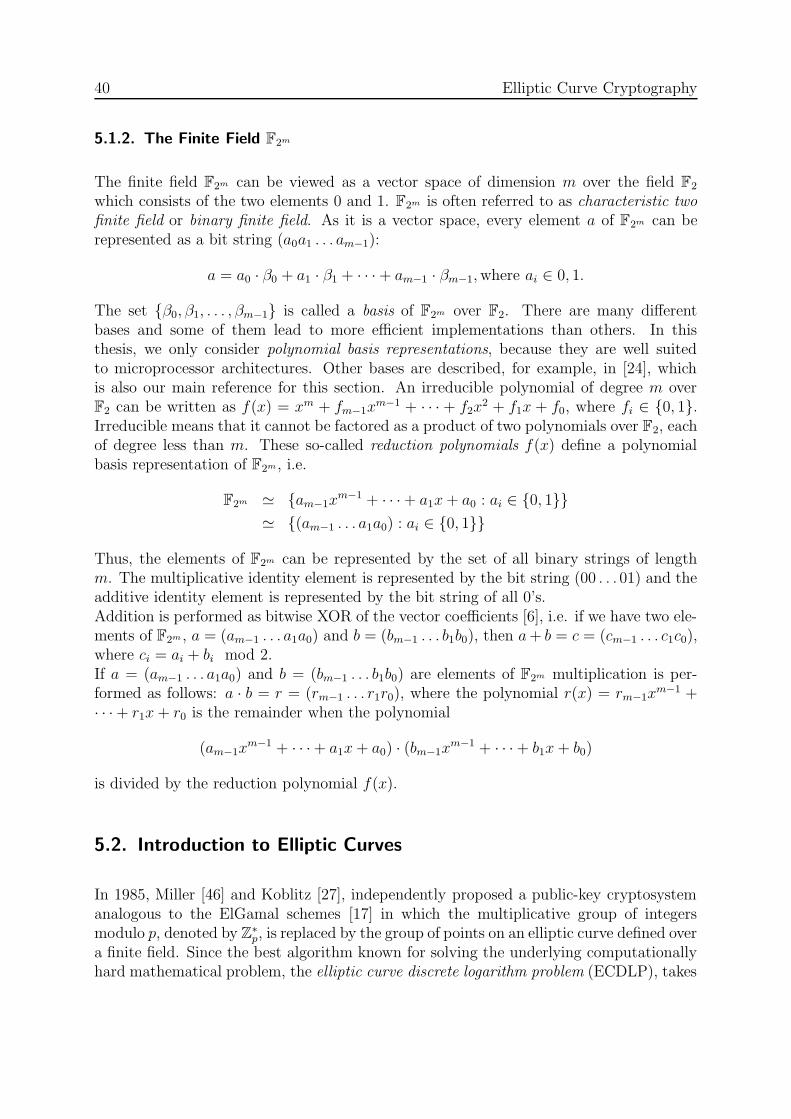
40 Elliptic Curve Cryptography
5.1.2. The Finite Field F2m
The finite field F2m can be viewed as a vector space of dimension m over the field F2
which consists of the two elements 0 and 1. F2m is often referred to as characteristic twofinite field or binary finite field. As it is a vector space, every element a of F2m can berepresented as a bit string (a0a1 . . . am−1):
a = a0 · β0 + a1 · β1 + · · ·+ am−1 · βm−1, where ai ∈ 0, 1.
The set {β0, β1, . . . , βm−1} is called a basis of F2m over F2. There are many differentbases and some of them lead to more efficient implementations than others. In thisthesis, we only consider polynomial basis representations, because they are well suitedto microprocessor architectures. Other bases are described, for example, in [24], whichis also our main reference for this section. An irreducible polynomial of degree m overF2 can be written as f(x) = xm + fm−1x
m−1 + · · · + f2x2 + f1x + f0, where fi ∈ {0, 1}.
Irreducible means that it cannot be factored as a product of two polynomials over F2, eachof degree less than m. These so-called reduction polynomials f(x) define a polynomialbasis representation of F2m, i.e.
F2m ' {am−1xm−1 + · · ·+ a1x + a0 : ai ∈ {0, 1}}
' {(am−1 . . . a1a0) : ai ∈ {0, 1}}
Thus, the elements of F2m can be represented by the set of all binary strings of lengthm. The multiplicative identity element is represented by the bit string (00 . . . 01) and theadditive identity element is represented by the bit string of all 0’s.Addition is performed as bitwise XOR of the vector coefficients [6], i.e. if we have two ele-ments of F2m , a = (am−1 . . . a1a0) and b = (bm−1 . . . b1b0), then a + b = c = (cm−1 . . . c1c0),where ci = ai + bi mod 2.If a = (am−1 . . . a1a0) and b = (bm−1 . . . b1b0) are elements of F2m multiplication is per-formed as follows: a · b = r = (rm−1 . . . r1r0), where the polynomial r(x) = rm−1x
m−1 +· · ·+ r1x + r0 is the remainder when the polynomial
(am−1xm−1 + · · ·+ a1x + a0) · (bm−1x
m−1 + · · ·+ b1x + b0)
is divided by the reduction polynomial f(x).
5.2. Introduction to Elliptic Curves
In 1985, Miller [46] and Koblitz [27], independently proposed a public-key cryptosystemanalogous to the ElGamal schemes [17] in which the multiplicative group of integersmodulo p, denoted by Z
∗p, is replaced by the group of points on an elliptic curve defined over
a finite field. Since the best algorithm known for solving the underlying computationallyhard mathematical problem, the elliptic curve discrete logarithm problem (ECDLP), takes

5.3 Arithmetic on General Elliptic Curves over F2m 41
fully exponential time, whereas the best algorithms known for solving the underlyingcomputationally hard mathematical problems in RSA (integer factorization problem) andDSA (the discrete logarithm problem) take sub-exponential time, significantly smallerparameters can be used in elliptic curve cryptography (ECC) than in other systems suchas RSA and DSA. For example, a 163-bit ECC key has a comparable level of security(against known attacks) as RSA and DSA with a modulus of 1024 bits [36]. This means byusing ECC one can reach the same level of security with less expense of processing power,storage space, bandwidth and electrical power, which makes it especially interesting forapplications on constrained devices such as smartcards, mobile phones and handhelds.
The performance of ECC depends mainly on the efficiency of finite field computationsand fast algorithms for elliptic scalar multiplications. Selecting particular underlyingfields and/or elliptic curves also speeds up the implementation. In Section 5.1, we alreadygave examples of such finite fields. Examples of families of curves that offer computationaladvantages are Koblitz curves over F2m .
Let us now introduce the mathematical definition of the elliptic curves we will workwith in the following. Suppose we have a finite field F2m . Then, the polynomial equation
E : y2 + xy = x3 + ax2 + b, (5.1)
with coefficients a, b ∈ F2m together with the point at infinity O define an elliptic curveover F2m . Let us ask for solutions (x, y) with x, y ∈ F2m . Such a solution is called pointon the elliptic curve E.
5.3. Arithmetic on General Elliptic Curves over F2m
The elliptic curve digital signature algorithm (ECDSA, see Section 3.3 for details) is basedon multiplying a point P on an elliptic curve with a scalar k. This is the nothing else thana k-fold addition of P . Hence, addition and scalar multiplication of points are importantarithmetic operations, which for this reason will be described in the following.
5.3.1. Point Addition
There is an illustrative way to explain the law for adding two points on an elliptic curve.Let us assume that the coefficients of our elliptic curve E as well as x and y are rationalnumbers. Then, we can certainly draw the curve E which is the set of all solutions (x, y)of Equation (5.1).
Starting with two distinct rational points P and Q on E, we draw a line through Pand Q and obtain a third point of intersection of the line with the curve. Reflecting thispoint in the x-axis, we obtain a point R, which we define to be the result of adding P +Q(see Figure 5.3.1). Since the line, the curve and the points of intersection are rational, Rmust also be rational.

42 Elliptic Curve Cryptography
Figure 5.3.1 Adding two points on an elliptic curve [24].
Even if we only have one rational point P , we can still generally get another one bydrawing the tangent line to the curve at P . This line will intersect with another point onthe curve. If we then reflect this point in the x-axis we obtain the point R = 2P , whichwill also be rational (see Figure 5.3.2).
Figure 5.3.2 Doubling a point on an elliptic curve [24].
One can show that together with a zero element O, these operations form a group. Letus agree on the convention that the points on our elliptic curve consist of the ordinary

5.3 Arithmetic on General Elliptic Curves over F2m 43
points in the ordinary affine x-y-plane together with a point O at infinity. We will callthis point point at infinity.
Addition using affine coordinates
Let us assume that P1 = (x1, y1) and P2 = (x2, y2) with O 6= P1 6= −P2 6= O aretwo distinct points on the curve E given by Equation (5.1). Based on the previouslymentioned geometric motivation one can derive the following formulas [19] for computingthe coordinates of the point P3 = P1 + P2 = (x3, y3). Note that we are in F2m , i.e.a, b, xi, yi ∈ F2m :
λ =
{ y1+y2
x1+x2if P1 6= P2
y1
x1+ x1 if P1 = P2
x3 = λ2 + λ + x1 + x2 + ay3 = (x1 + x3)λ + x3 + y1
(5.2)
The solutions for the two trivial cases Pj = O and P1 = −P2, which we have excludedabove, are straightforward, namely Pi +O = Pi and P1 + (−P2) = O, respectively.
In order to estimate and compare the computational cost of the following algorithms,which will use above equations to add two points in affine coordinates, let us examinethe equations with respect to the required number of field operations. Obviously, theformulas require 1 field division and 1 field multiplication. The computational cost offield additions and squarings can be neglected, since they can be done much faster thaninversion or multiplication (see Table 6.3.1 in Section 6.3.3 for concrete execution timeson our target platform).
Addition using projective coordinates / mixed coordinates
As inversion in F2m is computationally expensive relative to multiplication, it turns outthat representing a point using projective coordinates might be advantageous. There existseveral types of projective coordinates. In standard projective coordinates one finds thatthe projective point (X, Y, Z), Z 6= 0 corresponds to the affine point (x, y) = (X/Z, Y/Z).Then, the projective equation of the elliptic curve is Y 2Z + XY Z = X3 + aX2Z + bZ3.
In [37] a different set of projective coordinates is introduced that leads to computation-ally fast point arithmetic. The underlying map is the following
{(X, Y, Z) : Z 6= 0} 7−→{
(x, y) =
(X
Z,
Y
Z2
)}
{(X, Y, 0)} 7−→ O
and
{(x, y)} 7−→ {(X, Y, Z) = (x, y, 1)}O 7−→ {(α1, α2, 0), for any αi}

44 Elliptic Curve Cryptography
The projective equation of the elliptic curve is
Y 2 + XY Z = X3Z + aX2Z2 + bZ4. (5.3)
The addition of two points using mixed coordinates, i.e. one point given in affine coordi-nates and the other in projective coordinates, is especially of use in point multiplicationmethods presented later in this thesis. Here are the computation steps for a projectivepoint P1 = (X1, Y1, Z1) and an affine point P2 = (x2, y2) in the non-trivial case withO 6= P1 6= −P2 6= O. The result is the projective point P3 = P1 + P2 = (X3, Y3, Z3).
A = y2 · Z21 + Y1 B = x2 · Z1 + X1 C = Z1 ·B
D = B2 · (C + aZ21) Z3 = C2 E = A · C
X3 = A2 + D + E F = X3 + x2 · Z3 G = X3 + y2 · Z3
Y3 = E · F + Z3 ·G(5.4)
This operation requires 10 field multiplications, which on most platforms is faster thanaddition in affine coordinates (1 field multiplication plus 1 field division). On our SharpZaurus platform, the execution times are 121 � s vs. 158 � s (Table 6.4.1).
Doubling a projective point, i.e. calculating P3 = P1 + P1, can be done using thefollowing formulas:
Z3 = X21 · Z2
1
X3 = X41 + b · Z4
1
Y3 = bZ41 · Z3 + X3 · (aZ3 + Y 2
1 + bZ41)
(5.5)
This operation requires 5 field multiplications.
5.3.2. Scalar Point Multiplication
The computation of kP , where k is an integer and P is an elliptic curve point, is thebasic operation of cryptographic schemes based on elliptic curves. It also dominates theexecution time of those schemes. Thus, using efficient algorithms for point multiplicationhas a strong influence on the performance of elliptic curve cryptosystems. [19] presents agood overview over fast multiplication algorithms. In the following, we will describe thealgorithms we implemented.
Binary method
The simplest method for multiplying kP is based on the repeated-square-and-multiplymethod for exponentiation. Algorithm 5.3.1 shows how it works.

5.3 Arithmetic on General Elliptic Curves over F2m 45
Algorithm 5.3.1 Left-to-right binary method for point multiplication [19].
INPUT: k = (km−1, . . . , k1, k0)2, P ∈ F2m .OUTPUT: kP .
1: Q←− O.2: for i = m− 1 downto 0 do3: Q←− 2Q.4: if ki = 1 then5: Q←− Q + P .6: return Q.
P is usually given in affine coordinates. In order to minimize the number of computa-tionally expensive field inversions, we store Q in projective coordinates. The doubling inStep 3 is done as in Equations (5.5). For the addition in Step 5, we use Equations (5.4)to add P in affine coordinates to Q in projective coordinates.
Assuming that the average number of ones in the binary representation of k is m/2and neglecting the fact that the very first point doubling is simply a doubling of O, thealgorithm requires approximately m point doublings and m/2 point additions. Usingthe computational complexity in terms of finite field operations derived for the pointaddition methods, we can also express the complexity of this multiplication method interms of field multiplications and field divisions. The expected number of multiplicationsis (5m + 10 · (m/2)) = 10m. Another multiplication and division is necessary to convertthe result back to affine coordinates.
NAF and width-w NAF methods
The binary method can be sped up by using a different representation for k [59], theso-called nonadjacent form (NAF). This is a signed binary expansion with the propertythat no two consecutive coefficients are nonzero. For example,
NAF(29) = (1, 0, 0,−1, 0, 1)
since 29 = 32− 4 + 1. Every positive integer has a unique NAF. The NAF has the fewestnonzero coefficients of any signed binary expansion and it is at most one coefficient longerthan the binary representation [48].
The NAF can be generalized to the so-called width-w NAF that additionally increasesexecution speed. For any w > 1, each positive integer has a unique width-w NAF, denotedby NAFw(n):
n =
l−1∑
j=0
uj2j

46 Elliptic Curve Cryptography
where each uj is odd, |uj| < 2w−1 and among any w consecutive coefficients at most oneis nonzero. Algorithm 5.3.2 shows how NAFw(n) can be computed.In Step 4 of Algorithm 5.3.2, the expression ”k mods 2w” denotes the integer u satisfyingu ≡ k (mod 2w) and −2w−1 ≤ u < 2w−1. The actual implementation of Step 4 involvessome binary-bit arithmetic. The idea behind it is that k mods 2w is a signed integerrepresentation of the rightmost w bits. Therefore, we just isolate the rightmost w bits,extend the sign to a 32-bit value and get u as the result. Note that the subtraction inStep 5 is not a simple XOR-operation, but a long integer subtraction with borrow.
Algorithm 5.3.2 Computing the width-w NAF of a positive integer [19].
INPUT: A positive integer k.OUTPUT: NAFw(k).
1: i←− 0.2: while k ≥ 1 do3: if k is odd then4: ki ←− k mods 2w.5: k ←− k − ki.6: else7: ki ←− 0.8: k ←− k � 1.9: i←− i + 1.
10: return (ki−1, ki−2, . . . , k1, k0).
Algorithm 5.3.3 finally illustrates how point multiplication is done using the width-w NAF. For the point subtraction in Step 9, we use the fact that if P = (x, y) then−P = (x, x + y). After performing this operation the remaining addition is again doneaccording to Equations (5.4).
Algorithm 5.3.3 Window NAF method for point multiplication [19].
INPUT: Window width w, NAFw(k) =∑l−1
i=0 ki · 2i, P ∈ E(F2m).OUTPUT: kP .
1: Precompute Pi = iP , for i ∈ {1, 3, 5, . . . , 2w−1 − 1}.2: Q←− O.3: for i = l − 1 downto 0 do4: Q←− 2Q.5: if ki 6= 0 then6: if ki > 0 then7: Q←− Q + Pki
8: else9: Q←− Q− Pki
10: return Q.
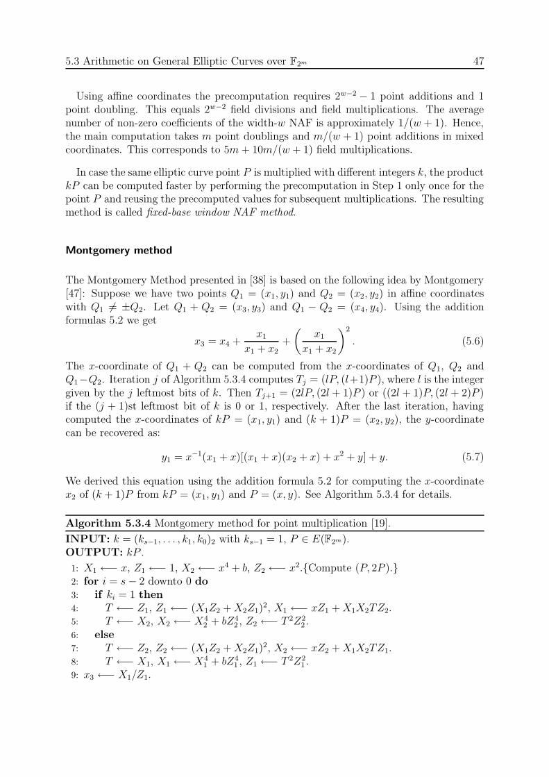
5.3 Arithmetic on General Elliptic Curves over F2m 47
Using affine coordinates the precomputation requires 2w−2 − 1 point additions and 1point doubling. This equals 2w−2 field divisions and field multiplications. The averagenumber of non-zero coefficients of the width-w NAF is approximately 1/(w + 1). Hence,the main computation takes m point doublings and m/(w + 1) point additions in mixedcoordinates. This corresponds to 5m + 10m/(w + 1) field multiplications.
In case the same elliptic curve point P is multiplied with different integers k, the productkP can be computed faster by performing the precomputation in Step 1 only once for thepoint P and reusing the precomputed values for subsequent multiplications. The resultingmethod is called fixed-base window NAF method.
Montgomery method
The Montgomery Method presented in [38] is based on the following idea by Montgomery[47]: Suppose we have two points Q1 = (x1, y1) and Q2 = (x2, y2) in affine coordinateswith Q1 6= ±Q2. Let Q1 + Q2 = (x3, y3) and Q1 − Q2 = (x4, y4). Using the additionformulas 5.2 we get
x3 = x4 +x1
x1 + x2+
(x1
x1 + x2
)2
. (5.6)
The x-coordinate of Q1 + Q2 can be computed from the x-coordinates of Q1, Q2 andQ1−Q2. Iteration j of Algorithm 5.3.4 computes Tj = (lP, (l+1)P ), where l is the integergiven by the j leftmost bits of k. Then Tj+1 = (2lP, (2l + 1)P ) or ((2l + 1)P, (2l + 2)P )if the (j + 1)st leftmost bit of k is 0 or 1, respectively. After the last iteration, havingcomputed the x-coordinates of kP = (x1, y1) and (k + 1)P = (x2, y2), the y-coordinatecan be recovered as:
y1 = x−1(x1 + x)[(x1 + x)(x2 + x) + x2 + y] + y. (5.7)
We derived this equation using the addition formula 5.2 for computing the x-coordinatex2 of (k + 1)P from kP = (x1, y1) and P = (x, y). See Algorithm 5.3.4 for details.
Algorithm 5.3.4 Montgomery method for point multiplication [19].
INPUT: k = (ks−1, . . . , k1, k0)2 with ks−1 = 1, P ∈ E(F2m).OUTPUT: kP .
1: X1 ←− x, Z1 ←− 1, X2 ←− x4 + b, Z2 ←− x2.{Compute (P, 2P ).}2: for i = s− 2 downto 0 do3: if ki = 1 then4: T ←− Z1, Z1 ←− (X1Z2 + X2Z1)
2, X1 ←− xZ1 + X1X2TZ2.5: T ←− X2, X2 ←− X4
2 + bZ42 , Z2 ←− T 2Z2
2 .6: else7: T ←− Z2, Z2 ←− (X1Z2 + X2Z1)
2, X2 ←− xZ2 + X1X2TZ1.8: T ←− X1, X1 ←− X4
1 + bZ41 , Z1 ←− T 2Z2
1 .9: x3 ←− X1/Z1.

48 Elliptic Curve Cryptography
10: y3 ←− (x + X1/Z1)[(X1 + xZ1)(X2 + xZ2) + (x2 + y)Z1Z2](xZ1Z2)−1 + y.
11: return (x3, y3).
The loop in Algorithm 5.3.4 takes 6m field multiplications and Steps 9 and 10 sum upto 7 field multiplications and 2 field divisions.
Comb method
In the comb method, proposed in [34], the basic idea is to write the binary representationof the scalar k in w rows and to process the columns of the resulting rectangle one columnat a time.
Algorithm 5.3.5 Comb method for point multiplication [19]
INPUT: Window width w, d = ds/we, k = (ks−1, . . . , k1, k0)2, P ∈ E(F2m).OUTPUT: kP .
1: Precompute Pn =∑w−1
i=0 ni2i·dP for 0 ≤ n < 2w, where nj is bit j in the binary
representation of n = (nw−1, . . . , n0)2 (see Algorithm 6.4.1).2: By padding k on the left with 0’s if necessary, write k = Kw−1‖ . . . ‖K1‖K0, where
each Kj is bit string of length d. Let Kji denote the ith bit of Kj.
3: Q←− O.4: for i = d− 1 downto 0 do5: Q←− 2Q.6: Q←− Q + P(Kw−1
i,...,K1
i,K0
i)2
.7: return Q.
Similar to the window NAF method, there is also a variant of this method for fixedpoints P , which performs the precomputation in Step 1 only once. This variant is calledfixed-base comb method. Neglecting the computational steps for the precomputation, thecalculation of kP requires d point doublings in projective coordinates and d point additionsin mixed coordinates. The sum of field multiplications is (5+10)d = 15d ≈ 15m
32w. However,
this requires memory for the storage of 2w − 1 precomputed elliptic curve points, whichmight be a serious disadvantage on some constrained devices.
Table 5.3.1 summarizes the complexity of the above mentioned multiplication methodsfor points on general elliptic curves over F2m . Obviously, the Montgomery method yieldsthe best performance among all methods for arbitrary points, whereas the fixed-base combmethod is the best choice among all fixed-base methods.

5.4 Arithmetic on Koblitz Elliptic Curves 49
Table 5.3.1 Estimated computational complexity of different multiplication methods interms of finite field operations.
Multiplication Method Number of Number ofField Multiplications Field Divisions
Arbitrary Point MethodsBinary Method 10m -Montgomery Method 6m + 7 2Window NAF Method 2w−2 + 5m + 10m/(w + 1) 2w−2
Fixed Point MethodsFixed-base Window NAF Method 5m + 10m/(w + 1) -Fixed-base Comb Method (15/32)m/w -
5.4. Arithmetic on Koblitz Elliptic Curves
In 1991, Koblitz presented a paper [28] in which he examines a subclass of binary ellip-tic curves with properties that allow for the use of efficient algorithms for scalar pointmultiplication. This type of curves is called Koblitz curve and they are defined by theequation
Ea : y2 + xy = x3 + ax2 + 1, (5.8)
where a ∈ F2, i.e. a ∈ {0, 1}. Obviously, the difference between general binary ellipticcurves and Koblitz curves is that the choice for the coefficients in the defining equation islimited to the set {0, 1}. Koblitz discovered interesting properties of these curves that canbe used to compute the point multiplication more efficiently. In this section, we introducesome of the theory that was summarized by Solinas in [59].
5.4.1. Basic Properties
The coefficients of Koblitz curves are either 0 or 1. Koblitz curves have the property thatif P = (x, y) is a point on Ea then so is the point (x2, y2) [59]. Hence, one finds
(x4, y4) + 2(x, y) = µ · (x2, y2) (5.9)
for every point (x, y) on the curve Ea, where µ := (−1)1−a.
Using the Frobenius map τ(x, y) := (x2, y2), τ(O) := O this can be written symbolically
(τ 2 + 2)P = µτP, (5.10)
where P is some point on the Koblitz curve.

50 Elliptic Curve Cryptography
Note that the Frobenius map is a very cheap operation from the computational pointof view. It only requires squaring the point coordinates and this can be done in only afraction of the time a field multiplication or division takes (see Section 6.3.1 for details).
The Frobenius map can be regarded as the complex number τ satisfying τ 2 + 2 = µτ ,
namely τ = µ+√−7
2. We can now represent the scalar k in our point multiplication
operation as an element of the ring Z[τ ]: k =∑l−1
i=0 uiτi. Consequently, we can multiply
points on the Koblitz curve by such an element
kP = (ul−1τl−1 + · · ·+ u1τ + u0)P = ul−1τ
l−1(P ) + · · ·+ u1τ(P ) + u0P (5.11)
Efficient point multiplication methods can now be developed by finding a nice represen-tation k =
∑l−1i=0 uiτ
i where l is relatively small and the coefficients ui are small andsparse.
Before describing the multiplication algorithms, let us introduce the so-called Lucassequences as we will need them later in this section. They are defined as follows:
U0 = 0, U1 = 1 and Uk+1 = µUk − 2Uk−1 for k ≥ 1;V0 = 2, V1 = µ and Vk+1 = µVk − 2Vk−1 for k ≥ 1.
(5.12)
Tables 5.4.1 summarizes some important definitions and relations for Koblitz curves,which we will need in the following.
Table 5.4.1 Important definitions and relations for Koblitz curves.
Definitionµ := (−1)1−a
τ(x, y) := (x2, y2)
Relation
f =
{2 for a = 14 for a = 0
τ 2 + 2 = µτU0 = 0, U1 = 1 and Uk+1 = µUk − 2Uk−1 for k ≥ 1V0 = 2, V1 = µ and Vk+1 = µVk − 2Vk−1 for k ≥ 1
5.4.2. Point Multiplication
τ-addic NAF (TNAF) multiplication method
Using the fact that τ 2+2 = µτ , one can show that every element in Z[τ ] can be expressed incanonical form r0+r1τ . Algorithm 5.4.1 takes an element κ in this representation as input

5.4 Arithmetic on Koblitz Elliptic Curves 51
and calculates its so-called τ -addic NAF (TNAF) κ =∑l−1
i=0 uiτi. In this representation
the coefficients ui are either 0 or ±1, and no two consecutive coefficients ui are nonzero.Note, that this algorithm involves multi-precision integer arithmetic.
Algorithm 5.4.1 Computing the τ -addic NAF of an element in Z[τ ][19]
INPUT: κ = r0 + r1τ ∈ Z[τ ].OUTPUT: TNAF(κ).
1: i←− 0.2: while r0 6= 0 OR r1 6= 0 do3: if r0 is odd then4: ui ←− 2− (r0 − 2r1 mod 4).5: r0 ←− r0 − ui.6: else7: ui ←− 0.8: t←− r0/2.9: r0 ←− r1 + µt.
10: r1 ←− −t.11: i←− i + 1.12: return (ui−1, ui−2, . . . , u1, u0).
Each κ ∈ Z[τ ] has a unique τ -addic NAF. For example for a = 1, we find
TNAF(9) = (1, 0,−1, 0, 0, 1),
since we can write 9 = τ 5−τ 3 +1. However, it turns out that the length of such a τ -addicNAF is approximately l(k) ≈ 2 log2 k and therefore twice as long as the length of thenormal NAF (introduced in Section 5.3.2).
The solution to this problem is an additional modular reduction step ρ = κ mod ((τm−1)/(τ − 1)), which is similar to the modular reduction of integers. In this formula, thevariable m is the m in F2m . Algorithm 5.4.2 shows how this modular reduction step canbe done in an efficient way. Note, that we do not exactly compute the modular reduction,but an approximation, the so-called partial modular reduction ρ′ = κ partmod ((τm −1)/(τ − 1)).
Algorithm 5.4.2 Computation of the partial modular reduction of an element in Z[τ ][19]
INPUT: An integer k, 0 < k < n, C ≥ 2, the Lucas sequence Vm,
and s0, s1, where si = (−1)i
f(1− µUm+3−a−i).
OUTPUT: ρ′ = k partmod ((τm − 1)/(τ − 1)).
1: k′ ←− bk/2a−C+(m−9)/2c.2: for i = 0 to 1 do
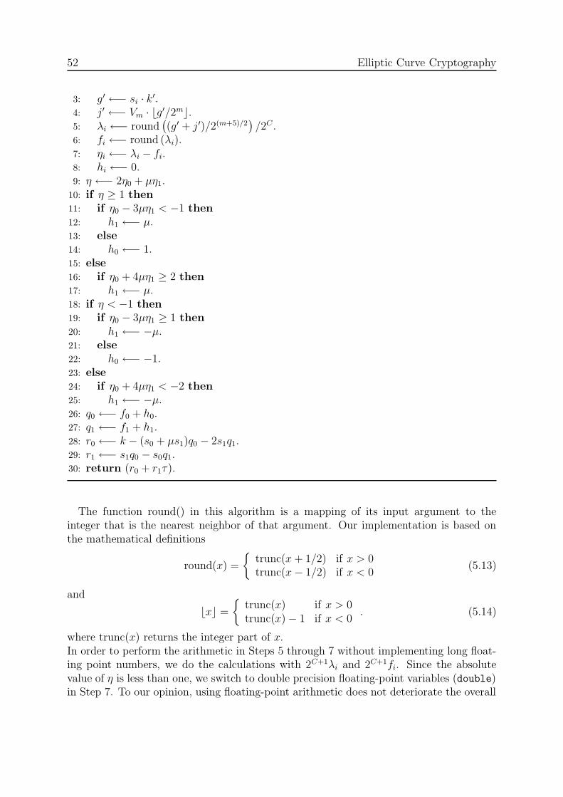
52 Elliptic Curve Cryptography
3: g′ ←− si · k′.4: j ′ ←− Vm · bg′/2mc.5: λi ←− round
((g′ + j ′)/2(m+5)/2
)/2C .
6: fi ←− round (λi).7: ηi ←− λi − fi.8: hi ←− 0.9: η ←− 2η0 + µη1.
10: if η ≥ 1 then11: if η0 − 3µη1 < −1 then12: h1 ←− µ.13: else14: h0 ←− 1.15: else16: if η0 + 4µη1 ≥ 2 then17: h1 ←− µ.18: if η < −1 then19: if η0 − 3µη1 ≥ 1 then20: h1 ←− −µ.21: else22: h0 ←− −1.23: else24: if η0 + 4µη1 < −2 then25: h1 ←− −µ.26: q0 ←− f0 + h0.27: q1 ←− f1 + h1.28: r0 ←− k − (s0 + µs1)q0 − 2s1q1.29: r1 ←− s1q0 − s0q1.30: return (r0 + r1τ).
The function round() in this algorithm is a mapping of its input argument to theinteger that is the nearest neighbor of that argument. Our implementation is based onthe mathematical definitions
round(x) =
{trunc(x + 1/2) if x > 0trunc(x− 1/2) if x < 0
(5.13)
and
bxc =
{trunc(x) if x > 0trunc(x)− 1 if x < 0
. (5.14)
where trunc(x) returns the integer part of x.In order to perform the arithmetic in Steps 5 through 7 without implementing long float-ing point numbers, we do the calculations with 2C+1λi and 2C+1fi. Since the absolutevalue of η is less than one, we switch to double precision floating-point variables (double)in Step 7. To our opinion, using floating-point arithmetic does not deteriorate the overall

5.4 Arithmetic on Koblitz Elliptic Curves 53
performance in a noticeable way.The parameter C ensures that TNAF(ρ′) of the partially reduced element is not muchlonger than TNAF(ρ) of the reduced element. One can show that the length l(ρ) ≤ m+a
and for C ≥ 2 that l(ρ′) ≤ m + a + 3. The probability that ρ 6= ρ′ is less than(
12
)C−5.
Furthermore, we know that the average density of nonzero coefficients of such a TNAF isapproximately 1/3. Following the suggestion in [59], we chose C = 12 to obtain a goodperformance for our TNAF multiplication methods.
The above results lead to the following algorithm for scalar point multiplication onKoblitz curves, which has an expected running time of approximately m/3 point additionsin mixed coordinates. This corresponds to 10 ·m/3 = (10/3)m field multiplications.Note that Step 3 corresponds to simply squaring all three coordinates of Q.
Algorithm 5.4.3 TNAF method for point multiplication [19]
INPUT: TNAF(ρ′) =∑l−1
i=0 uiτi, where ρ′ = k partmod ((τm−1)/(τ−1)), P ∈ Ea(F2m).
OUTPUT: kP .
1: Q←− O.2: for i = l − 1 downto 0 do3: Q←− τQ.4: if ui = 1 then5: Q = Q + P .6: if ui = −1 then7: Q = Q− P .8: return Q.
Window TNAF multiplication method
Analogous to the width-w NAF multiplication method, we can extend the TNAF multi-plication method to a window method. Using the Lucas sequences Uw, let us define
tw := 2Uw−1U−1w mod 2w. (5.15)
One can show that the odd numbers ±1,±3, . . . ,±(2w−1−1) are incongruent modulo τw.For αi = i mod τw for i ∈ {1, 3, . . . , 2w−1 − 1}, the width-w TNAF of κ ∈ Z[τ ] is theexpression κ =
∑l−1i=0 uiτ
i, where ui ∈ {0,±α1,±α2, . . . ,±α2w−1−1}.
One key property of the width-w TNAF is that at most one of any w consecutivecoefficients is nonzero. Algorithm 5.4.4 is a simple method for computing TNAFw(κ).Note, that Step 4 is the same as in the computation of the width-w NAF. Hence, theimplementation of this step does not differ a lot from the corresponding step in thewindow NAF algorithm.

54 Elliptic Curve Cryptography
Algorithm 5.4.4 Computing the width-w TNAF of an element in Z[τ ][19]
INPUT: w, tw, αi = βi + γiτ for i ∈ {1, 3, . . . , 2w−1 − 1}, ρ = r0 + r1τ ∈ Z[τ ].OUTPUT: TNAFw(ρ).
1: i←− 0.2: while r0 6= 0 OR r1 6= 0 do3: if r0 is odd then4: u←− r0 + r1tw mods 2w.5: if u > 0 then6: s←− 1.7: else8: s←− −1.9: u←− −u.
10: r0 ←− r0 − sβu.11: r1 ←− r1 − sγu.12: ui ←− sαu.13: else14: ui ←− 0.15: t←− r0/2.16: r0 ←− r1 + µt.17: r1 ←− −t.18: i←− i + 1.19: return (ui−1, ui−2, . . . , u1, u0).
Among all width-w TNAFs of length l the average density of non-zero coefficients isapproximately 1/(w + 1). Using the partial modular reduction algorithm, we obtain awidth-w TNAF of length approximately l(ρ′). The following algorithm uses TNAFw(ρ′)to compute kP :
Algorithm 5.4.5 Window TNAF method for point multiplication [19]
INPUT: TNAFw(ρ′) =∑l−1
i=0 uiτi, where ρ′ = k partmod ((τm − 1)/(τ − 1)), P ∈
Ea(F2m).OUTPUT: kP .
1: Precompute Pu = αuP , for u ∈ {1, 3, . . . , 2w−1 − 1}.2: Q←− O.3: for i = l − 1 downto 0 do4: Q←− τQ.5: if ui 6= 0 then6: Let u be such that αu = ui or α−u = −ui.7: if u > 0 then8: Q = Q + Pu.9: else
10: Q = Q− P−u.

5.5 Known Attacks Against Elliptic Curve Cryptosystems 55
11: return Q.
The precomputation requires 2w−2 − 1 point additions in affine coordinates, whichcorresponds to 2w−2 − 1 field multiplications and divisions. The main multiplicationroutine has an expected running time of m/(w +1) point additions in mixed coordinates,which corresponds to 10 · m/(w + 1) field multiplications. Of course, for a fixed pointP , the precomputation needs only to be done once. In this case, we call the methodfixed-base window TNAF method.
Table 5.4.2 summarizes the complexity of the above mentioned multiplication methodsfor points on Koblitz curves. Comparing these results to the complexities of methods forgeneral elliptic curves over F2m (Table 5.3.1), one notices that the TNAF method is fasterthan the Montgomery Method. However, the window TNAF method is not faster thanthe fixed-base comb method for fixed points.
Table 5.4.2 Estimated computational complexity of different multiplication methods interms of finite field operations.
Multiplication Method Number of Number ofField Multiplications Field Divisions
Arbitary Point MethodsTNAF method (10/3)m -Window TNAF Method 10m/(w + 1) + 2w−2 − 1 2w−2 − 1Fixed Point MethodsFixed-base Window TNAF Method 10m/(w + 1) -
5.5. Known Attacks Against Elliptic Curve Cryptosystems
In this section, we present some known attacks against elliptic curve cryptosystems. Thescope of this section is limited to algorithms solving the elliptic curve discrete logarithmproblem (ECDLP), i. e. to determine l given a point P and a point Q = lP , and it doesnot consider attacks against particular elements of digital signature algorithms based onelliptic curves. The following enumeration and further references can be originally foundin [24].
1. Naive Exhaustive Search: The most simple approach to obtain l is to computesuccessive multiples of P : P, 2P, 3P, 4P, . . . until the result is equal to Q. In theworst case, this takes n steps, where n is the order of the point P .
2. Baby-Step Giant-Step Algorithm: This algorithm is a time-memory trade-offof the method of exhaustive search. It requires storage for about
√n points, and its
running time is roughly√
n steps in the worst case.

56 Elliptic Curve Cryptography
3. Pollard’s Rho Algorithm: This algorithm is a randomized version of the baby-step giant-step algorithm. With some modifications it can be sped up to have anexpected running time of
√πn/2 steps and it requires only a negligible amount of
storage.
4. Parallelized Pollard’s Rho Algorithm: The original Pollard’s rho algorithmcan be parallelized so that when it is run in parallel on r processors, the expectedrunning time is roughly
√πn/(2r).
5. Pollard’s Lambda Method: Pollard also presented a lambda method for comput-ing discrete logarithms which is applicable when l, the logarithm sought, is knownto lie in a certain interval. In particular, when l is known to lie in a subinterval [0, b]of [0, n − 1], where b < 0.39n, the parallelized version of Pollard’s lambda methodis faster than the parallelized Pollard’s rho algorithm.
6. Multiple Logarithms: It turns out that if a single instance of the ECDLP issolved using (parallelized) Pollard’s rho method, the following instances (for thesame curve E and the same base point P ) can be solved faster, since some ofthe necessary work has already been done in the previous steps. In fact, solvingk instances of the ECDLP takes only
√k as much work as it does to solve one
instance.
Hence, the best known attack against a single instance of the ECDLP is Pollard’s rhoalgorithm and has an expected running time of
√πn/2 = O(n1/2), which is fully expo-
nential.
However, there are certain elliptic curves with special vulnerabilities that can be ex-ploited by the following algorithms. These algorithms may have shorter running timesas those mentioned before, therefore elliptic curves with these vulnerabilities should beavoided. Further references can be found in [24] where the following list originates.
1. Pohlig-Hellman Algorithm: This algorithm exploits the factorization of n, theorder of the point P , and reduces the problem of recovering l to the problem ofrecovering l modulo each of the prime factors of n. We can then recover l by usingthe Chinese Remainder Theorem. As a countermeasure, one should select an ellipticcurve whose order is a prime or almost a prime (i. e. a large prime times a smallinteger).
2. Supersingular Elliptic Curves: In some cases, the ECDLP in an elliptic curveE defined over a finite field Fq can be reduced to the ordinary discrete logarithmproblem (DLP) in the multiplicative group of some extension field Fqk for k ≥ 1.The DLP is the underlying computationally hard mathematical problem for theDSA and one can solve it using the number field sieve algorithm, which has a sub-exponential running time. To ensure that the reduction algorithm does not applyto a particular curve, one only needs to check that n does not divide qk − 1 for allsmall k for which the DLP in Fqk is tractable. In practice, it suffices to check thisfor 1 ≤ k ≤ 20 when n > 2160.

5.5 Known Attacks Against Elliptic Curve Cryptosystems 57
3. Prime-Field Anomalous Curves: If the number of points on a curve E over Fp
is equal to p, the ECDLP can be solved efficiently. This attack can be avoided byverifying that the number of points on an elliptic curve is not equal to the cardinalityof the underlying field.
4. Curves Defined Over a Small Field: For elliptic curves E with coefficients inF2e , Pollard’s rho algorithm for computing elliptic curve logarithms in E(F2ed) canbe further sped up by a factor of
√d. For example, if E is a Koblitz curve, then
Pollard’s rho algorithm for computing elliptic curve logarithms in E(F2m) can besped up by a factor of
√m.
5. Curves Defined Over F2m, m Composite: The Weil descent might be used tosolve the ECDLP for elliptic curves defined over F2m where m is composite. Thereexists some evidence that when m has a small divisor l, e.g. l = 4, the ECDLPcan be solved faster than with Pollard’s rho algorithm. Thus, elliptic curves overcomposite fields should not be used.
Finally, let us examine how secure elliptic curve cryptography is in practice. One sourcethat gives a notion about the security of ECC is the Certicom challenge [42]. The challengeis to compute the ECC private keys from a given list of ECC public keys and associatedsystem parameters. The challenge has been issued in November 1997 and consists of twolevels:
� Level I: 109-bit and 131-bit challenge; considered to be feasible
� Level II: 163-bit, 191-bit, 239-bit and 359-bit challenge; expected to be computa-tionally infeasible
Of the Level I challenges, the 109-bit ECC2K-108 challenge has been solved in April2000 and the 109-bit ECCp-109 challenge has been solved in November 2002. All otherchallenges are (until March 2003) unsolved. According to Certicom, the computationalcost to solve these challenges met the expected values.
Concrete recommendations based on the expected cost of the Certicom challenge havebeen presented by Lenstra and Verheul in [33]. Using a model that incorporates tech-nological and cryptanalytical advances they predict which elliptic curve key sizes can beconsidered as secure until which year. Elliptic curves with a key size of 140-bit, for exam-ple, shall provide a sufficient level of security for commercial applications until the year2003. The authors assume that a computational cost of about 3.5 ·1010 Mips years can beconsidered to be infeasible until the year 2003. Table 5.5.1 presents their recommendationsfor future years.

58 Elliptic Curve Cryptography
Table 5.5.1 Minimum key size for elliptic curve cryptosystems providing a sufficient levelof security [33].
YearElliptic Curve
Key SizeInfeasible Number
of Mips Years
CorrespondingNumber of Years
on 450MHzPentium II PC
2002 139 2.06 · 1010 4.59 · 107
2003 140 3.51 · 1010 7.80 · 107
2004 143 5.98 · 1010 1.33 · 108
2005 147 1.02 · 1011 2.26 · 108
2006 148 1.73 · 1011 3.84 · 108
2007 152 2.94 · 1011 6.54 · 108
2008 155 5.01 · 1011 1.11 · 109
2009 157 8.52 · 1011 1.89 · 109
2010 160 1.45 · 1012 3.22 · 109
2011 163 2.47 · 1012 5.48 · 109
2012 165 4.19 · 1012 9.32 · 109
2013 168 7.14 · 1012 1.59 · 1010
2014 172 1.21 · 1013 2.70 · 1010
2015 173 2.07 · 1013 4.59 · 1010
2016 177 3.51 · 1013 7.81 · 1010
2017 180 5.98 · 1013 1.33 · 1011
2018 181 1.02 · 1014 2.26 · 1011
2019 185 1.73 · 1014 3.85 · 1011
2020 188 2.94 · 1014 6.54 · 1011
2021 190 5.01 · 1014 1.11 · 1012
2022 193 8.52 · 1014 1.89 · 1012
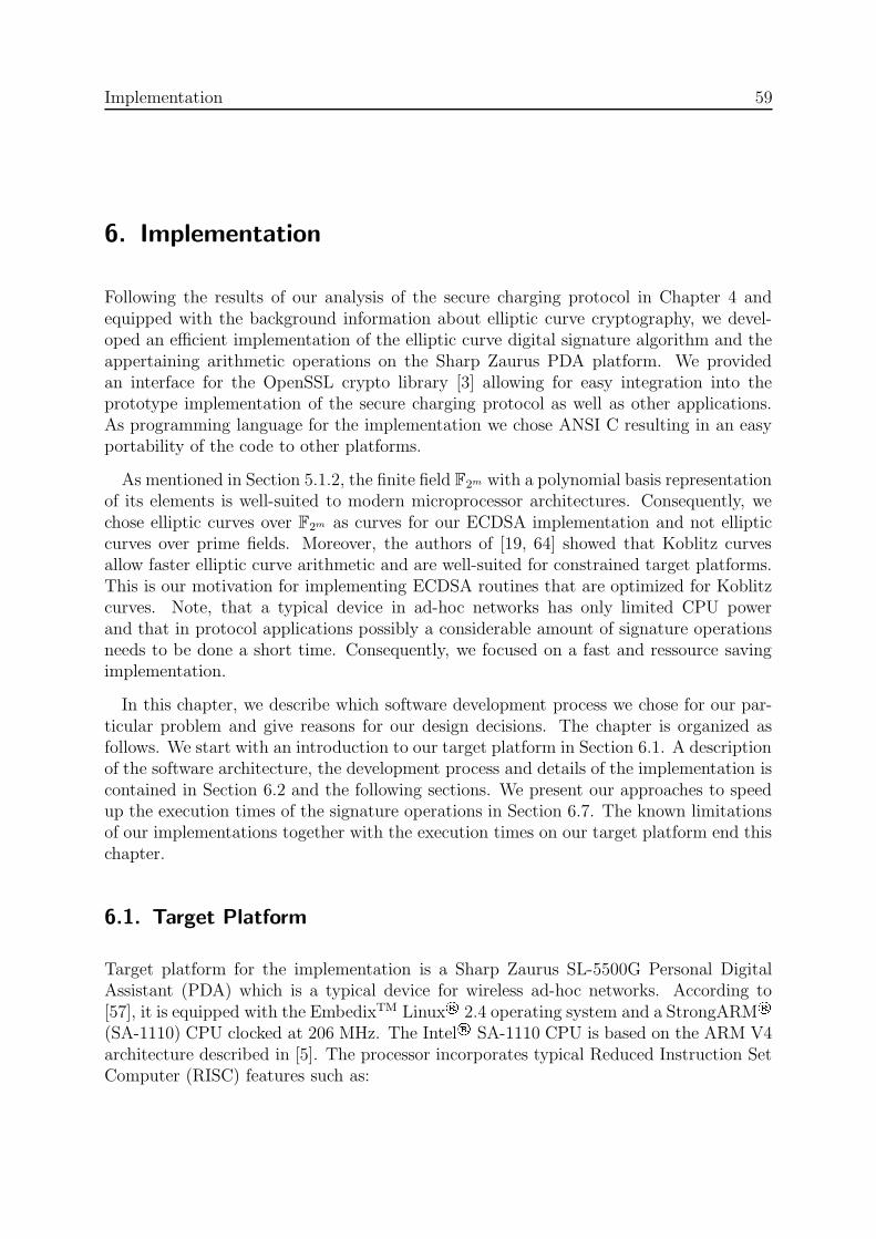
Implementation 59
6. Implementation
Following the results of our analysis of the secure charging protocol in Chapter 4 andequipped with the background information about elliptic curve cryptography, we devel-oped an efficient implementation of the elliptic curve digital signature algorithm and theappertaining arithmetic operations on the Sharp Zaurus PDA platform. We providedan interface for the OpenSSL crypto library [3] allowing for easy integration into theprototype implementation of the secure charging protocol as well as other applications.As programming language for the implementation we chose ANSI C resulting in an easyportability of the code to other platforms.
As mentioned in Section 5.1.2, the finite field F2m with a polynomial basis representationof its elements is well-suited to modern microprocessor architectures. Consequently, wechose elliptic curves over F2m as curves for our ECDSA implementation and not ellipticcurves over prime fields. Moreover, the authors of [19, 64] showed that Koblitz curvesallow faster elliptic curve arithmetic and are well-suited for constrained target platforms.This is our motivation for implementing ECDSA routines that are optimized for Koblitzcurves. Note, that a typical device in ad-hoc networks has only limited CPU powerand that in protocol applications possibly a considerable amount of signature operationsneeds to be done a short time. Consequently, we focused on a fast and ressource savingimplementation.
In this chapter, we describe which software development process we chose for our par-ticular problem and give reasons for our design decisions. The chapter is organized asfollows. We start with an introduction to our target platform in Section 6.1. A descriptionof the software architecture, the development process and details of the implementation iscontained in Section 6.2 and the following sections. We present our approaches to speedup the execution times of the signature operations in Section 6.7. The known limitationsof our implementations together with the execution times on our target platform end thischapter.
6.1. Target Platform
Target platform for the implementation is a Sharp Zaurus SL-5500G Personal DigitalAssistant (PDA) which is a typical device for wireless ad-hoc networks. According to[57], it is equipped with the EmbedixTM Linux
�2.4 operating system and a StrongARM
�
(SA-1110) CPU clocked at 206 MHz. The Intel�
SA-1110 CPU is based on the ARM V4architecture described in [5]. The processor incorporates typical Reduced Instruction SetComputer (RISC) features such as:

60 Implementation
� 31 general-purpose 32-bit registers. 16 of them are visible at a time, the others areused to speed up exception processing. Of the visible registers 14 can freely be used,the remaining two are reserved as program counter and return address storage
� A load/store architecture, where data-processing only operates on register contents,not directly on memory contents
� Uniform and fixed-length instruction fields with conditional execution feature
� Arithmetic Logic Unit (ALU) and shifter can be controlled in every processing step
� Load and Store Multiple instructions maximize data throughput
The 32-bit register architecture motivates the usage of 32-bit word variables throughoutthe implementation.
The size of the memory is specified as 64 MB RAM and 16 MB flash ROM. TheRAM is further subdivided into 32 MB for processes, buffers, cache, and 32 MB foradditional file and directory storage [56]. Compared to usual desktop PCs this is very fewavailable memory, so one of the major goals of this thesis is to develop a fast but smallimplementation of the elliptic curve routines.
Our implementation is done in C. The compiler used for the development is a GNUcross-compiler supplied by EmbedixTM [2] that builds executables for the ARM V4 archi-tecture and Linux OS.
6.2. Software Architecture
After analyzing the structure of ECDSA, we feel that it is the best choice to use thebottom-up approach for developing the implementation. Hence, we organize the softwarein the following layered model (Figure 6.2.1).
The layers can be described as follows, starting from the lowest:
1. Finite Field and Long Integer Arithmetic LayerThe elliptic curve arithmetic is based on finite field arithmetic and in case of Koblitzcurves, it also needs long integer arithmetic. This layer provides an efficient imple-mentation of all necessary methods. It has a key influence on the performance ofall higher layers, therefore we decided to tailor our implementation to a particularfinite field. More details can be found in Section 6.3.
2. Elliptic Curve Arithmetic LayerThe Elliptic Curve Arithmetic Layer includes implementations of several differentmethods for scalar multiplication of points on an elliptic curve, the implementationof point addition in different types of coordinates (used by multiplication methodsand higher layers) and a couple of helper functions. Section 6.4 contains a detaileddescription of this layer.

6.2 Software Architecture 61
3. ECDSA Sign and Verify LayerThe next layer of our optimized implementation is the ECDSA Sign and VerifyLayer. It provides lightweight interfaces for the sign and verify operations as wellas initialization and precomputation routines. This layer is described in detail inSection 6.5.
4. OpenSSL Interface LayerThis layer embeds the optimized ECDSA implementation into the existing OpenSSLframework. The OpenSSL framework is organized in a modular manner, thereforethe integration of new methods or different implementations of existing methods isquite easy. We describe this process later on in Section 6.6.
Figure 6.2.1 Architecture Overview
OpenSSL Interface
ECDSA Sign and Verify
Elliptic Curve Arithmetic
Finite Field and Long Integer Arithmetic
Point Addition Point Multiplication
Finite Field Arithmetic Long Integer Arithmetic
The major advantage of implementing the lowest layer first and gradually combiningmodules is that testing and debugging becomes easier. The modules on the low layercan be tested and debugged separately from other components. Higher layer modules arenot developed before the modules on lower layers function correctly according to theirspecifications. Tests of these higher layer modules can rely on the correctness of theincorporated modules.
From the optimization point of view, the bottom-up approach is also very attractive.The functions on the lower layers of the model form the time critical part of the code, sincethey are usually executed more often than those on higher layers. We have the possibilityto determine the execution times of the isolated modules and can directly measure theinfluence of optimization approaches on their performance.

62 Implementation
6.3. Finite Field Arithmetic in F2m and Long Integer Arithmetic
6.3.1. Finite Field Arithmetic
The following explanations and our implementation of finite field arithmetic are mostlybased on [19] and [64]. The files g2fm_inline_gen.h, g2fm_inline.c, g2fm_gen.h,g2fm_gen.c, g2fm.h, and g2fm.c contain our implementation. The reasons for this filestructure are explained in Section 6.7, which treats our optimization approaches.
Field representation
As mentioned in [19] and in Section 5.1.2 of this document, the polynomial basis repre-sentation of F2m with a trinomial or pentanomial as a reduction polynomial f(x) appearsto yield the simplest and fastest implementation in software. Therefore, we use thisrepresentation throughout our implementation of finite field arithmetic.
Consequently, we write an element A ∈ F2m as polynomial A(x) =∑m−1
i=0 aixi and store
it as binary vector A = (am−1, . . . , a0). How to store these coefficients in computers isstraightforward: since they are binary values, one can store each coefficient in one bit ofmemory. Due to the 32-bit register architecture of the StrongARM CPU, we use an arrayof s = dm/32e 32-bit words (A[s − 1], . . . , A[0]). The rightmost bit of A[0] correspondsto a0 and am−1 is part of A[s− 1]. The bits left of am−1 are set to zero. For m = 163 anarray of s = 6 32-bit words would be sufficient.
We basically defined two types, namely gf2mShortElement and gf2mLongElement, thatare arrays of s and 2s words. The later type holds intermediate results of multiplicationsor squarings, while the first one is used for all other field elements.
Addition
As stated in Section 5.1.2, addition of field elements is performed by bitwise XOR oper-ations that will be denoted by ⊕. The ARM V4 architecture offers native 32-bit XORinstructions, thus addition should only require s operations.
Multiplication
The product c = a · b is computed by first evaluating c′(x) = a(x) · b(x) followed bymodular reduction c(x) ≡ c′(x) mod f(x).
Polynomial Multiplication
To our knowledge, Algorithm 6.3.1 is the fastest method to compute c = a · b. Itdoes this by using a window method [38]. In Step 1, polynomials Bu = u(x) · b(x) are

6.3 Finite Field Arithmetic in F2m and Long Integer Arithmetic 63
precomputed for 0 ≤ u ≤ 2w where w is the window size. This is done using a couple ofleft shifts and cumulative field element additions. In Steps 6 and 10 the m-bit vector Bu
is added to C where the rightmost bit of Bu is added to the rightmost bit of C{j}. Here,C{j} denotes the bit vector (C[2s−2], . . . , C[j]) and the symbol � denotes a bitwise leftshift. The result of the algorithm is not reduced, so c(x) is of degree at most 2m− 2.
Algorithm 6.3.1 Left-to-right comb method with windows of width w = 4 [19]
INPUT: Binary polynomials a(x) and b(x) of degree at most m− 1.OUTPUT: A binary polynomial c(x) = a(x)·b(x) of degree at most 2m−2.
1: Compute Bu = u(x) · b(x) for all polynomials u(x) of degree at most 3.2: C ←− 0.3: for k = 7 downto 1 do4: for j = 0 to s− 1 do5: Let u = (u3, u2, u1, u0), where ui is bit (4k + i) of A[j].6: C{j} ←− C{j} ⊕Bu.7: C{j} ←− C{j} � 4.8: for j = 0 to s−1 do {The case k = 0. This saves one comparison in the loop above.}9: Let u = (u3, u2, u1, u0), where ui is bit i of A[j].
10: C{j} ←− C{j} ⊕ Bu.11: return c(x).
Modular Reduction
By choosing the reduction polynomial f(x) to be a low weight polynomial, i.e. onewith the least possible number of non-zero coefficients, reduction modulo f(x) becomes acomputationally cheap operation [6]. For cases of practical interest, f(x) is a trinomial orpentanomial, i.e. the number of non-zero coefficients is 3 or 5. If the middle terms in f(x)are close to each other, then reduction of c(x) modulo f(x) can be efficiently performedone word at a time. Suppose f(x) = x163 + x7 + x6 + x3 + 1. Then
x163 ≡ x7 + x6 + x3 + 1 mod f(x)...
x288 ≡ x132 + x131 + x128 + x125 mod f(x)...
x324 ≡ x168 + x167 + x164 + x161 mod f(x)
Hence, reduction can be performed by adding to C properly aligned all those C[j] thatcontain the coefficients ck, 163 ≤ k ≤ 324.
Let us clarify this with an example. Suppose we have already reduced C[10] and nowwant to reduce C[9], which contains bits 288 through 319. We can write the corresponding
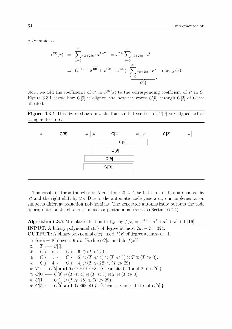
64 Implementation
polynomial as
c(9)(x) =
31∑
k=0
ck+288 · xk+288 = x28831∑
k=0
ck+288 · xk
≡ (x132 + x131 + x128 + x125) ·31∑
k=0
ck+288 · xk
︸ ︷︷ ︸
C[9]
mod f(x)
Now, we add the coefficients of xi in c(9)(x) to the corresponding coefficient of xi in C.Figure 6.3.1 shows how C[9] is aligned and how the words C[5] through C[3] of C areaffected.
Figure 6.3.1 This figure shows how the four shifted versions of C[9] are aligned beforebeing added to C.
C[5] C[4] C[3]
C[9]
C[9]
C[9]
C[9]
191 159 127160 128 96
The result of these thoughts is Algorithm 6.3.2. The left shift of bits is denoted by� and the right shift by �. Due to the automatic code generator, our implementationsupports different reduction polynomials. The generator automatically outputs the codeappropriate for the chosen trinomial or pentanomial (see also Section 6.7.4).
Algorithm 6.3.2 Modular reduction in F2m by f(x) = x163 + x7 + x6 + x3 + 1 [19]
INPUT: A binary polynomial c(x) of degree at most 2m− 2 = 324.OUTPUT: A binary polynomial c(x) mod f(x) of degree at most m−1.
1: for i = 10 downto 6 do {Reduce C[i] modulo f(x)}2: T ←− C[i].3: C[i− 6]←− C[i− 6]⊕ (T � 29).4: C[i− 5]←− C[i− 5]⊕ (T � 4)⊕ (T � 3)⊕ T ⊕ (T � 3).5: C[i− 4]←− C[i− 4]⊕ (T � 28)⊕ (T � 29).6: T ←− C[5] and 0xFFFFFFF8. {Clear bits 0, 1 and 2 of C[5].}7: C[0]←− C[0]⊕ (T � 4)⊕ (T � 3)⊕ T ⊕ (T � 3).8: C[1]←− C[1]⊕ (T � 28)⊕ (T � 29).9: C[5]←− C[5] and 0x00000007. {Clear the unused bits of C[5].}

6.3 Finite Field Arithmetic in F2m and Long Integer Arithmetic 65
10: return (C[5], C[4], C[3], C[2], C[1], C[0]).
Squaring
Squaring in F2m can be done much faster than multiplying two arbitrary elements. Itturns out to be a linear operation, because for a(x) =
∑m−1i=0 aix
i one finds
a2(x) =m−1∑
i=0
m−1∑
j=0
aiajxi+j =
m−1∑
i=0
aix2i
Hence, squaring can be done by simply inserting a 0-bit between consecutive bits of thebinary representation of a. A fast way to do that is to use a table of precomputed valuesas shown in Algorithm 6.3.3 [54], which is a static table in our implementation. Hence,the precomputation step needs not to be done during run-time. The reduction step isdone using Algorithm 6.3.2.
Algorithm 6.3.3 Squaring in F2m [54]
INPUT: A binary polynomial a(x) of degree at most m− 1.OUTPUT: A binary polynomial b(x) = a2(x) mod f(x) of degree at most m− 1.
1: Precompute for each byte v = (v7, . . . , v1, v0) the 16-bit vectorT (v) = (0, v7, . . . , 0, v1, 0, v0).
2: for i = 0 to s− 1 do3: Let A[i] = (u3, u2, u1, u0) where each uj is a byte.4: C[2i]←− (T (u1), T (u0)), C[2i + 1]←− (T (u3), T (u2)).5: Compute b(x) = c(x) mod f(x). {using Algorithm 6.3.2.}6: return b(x).
Modular division
Based on a paper by Sheueling Chang Shantz [55] Algorithm 6.3.4 is used to computethe modular division a
bdirectly, because the running time is roughly the same as the one
of the Extended Euclidean Algorithm that computes the modular inverse. By doing so,we save one modular multiplication. The comparison between two elements is done bytreating the 32-bit words as unsigned integers where A[i+1] is more significant than A[i].
Algorithm 6.3.4 Modular Division in F2m [55]
INPUT: Binary polynomials a(x) and b(x) 6= 0 of degree at most m− 1.
OUTPUT: A binary polynomial c(x) = a(x)b(x)
mod f(x) of degree at most m−1.

66 Implementation
1: A←− b, B ←− f , U ←− a, V ←− 0.2: while A 6= B do3: if A is even then4: A� 1.5: if U is odd then6: U ←− U ⊕ f .7: U � 1.8: else if B is even then9: B � 1.
10: if V is odd then11: V ←− V ⊕ f .12: V � 1.13: else if A > B then14: A←− A⊕B15: A� 1.16: U ←− U ⊕ V17: if U is odd then18: U ←− U ⊕ f19: U � 1.20: else21: B ←− A⊕B22: B � 1.23: V ←− U ⊕ V24: if V is odd then25: V ←− V ⊕ f26: V � 1.27: return U(x).
6.3.2. Long Integer Arithmetic
The implementation of point multiplication methods that are optimized for elliptic curvesof Koblitz type requires long integer arithmetic. Long integer arithmetic consists of arith-metic operations with integers that are longer than the 32-bit integers that are supportedby native CPU operations.

6.3 Finite Field Arithmetic in F2m and Long Integer Arithmetic 67
Long integer representation
We use the following structure to represent long integers:
typedef struct
{
Word32 *data;
bool bNegative;
unsigned int nWordsUsed;
unsigned int nWordsAllocated;
} longint;
The member data points to an array that contains the absolute value of the long integer.The least significant bit is bit 0 of data[0] and the most significant bit is bit 31 of the lastelement of the array. For performance reasons, data points mostly to statically allocatedmemory (on the stack), however, sometimes we also dynamically allocate memory onthe heap. The boolean bNegative contains the sign of the long integer, i.e. it is trueif the integer is a negative number. We chose the absolute value / sign representationinstead of the two’s complement representation, because for a sign inversion, the two’scomplement representation requires as many inversions as there are words whereas theabsolute value / sign representation requires only a change of the sign flag. The twomembers nWordsAllocated and nWordsUsed specify how many words of memory havebeen allocated for the absolute value of the long integer (the chunk of memory that datapoints to) and how much of it is really used. Hence, the last used element of the arrayis always data[nWordsUsed - 1]. This kind of design is necessary, on one hand forcompatibility reasons (OpenSSL uses a similar representation) and on the other hand inorder to represent long integers with many different lengths as they appear as intermediateresults of the Koblitz curve arithmetic.
Addition
We implemented the addition algorithm as it is given in [45], Algorithm 14.7. However,since we have to do signed multiprecision integer arithmetic, our routine also contains asign check that treats the following two cases separately:
1. Both operands have the same sign: Add the absolute values and set the sign of theresult to the common sign.
2. The signs of the operands are different: Subtract the absolute value of the operandwith the greater absolute value from the one with the smaller absolute value andset the sign of the result to the sign of the operand with greater absolute value.

68 Implementation
Another difficulty is how to correctly determine carries in the C programming language.It does not offer direct access to the carry flag of the processor, so we use the followingalgorithm:
Algorithm 6.3.5 Addition with carry detection in the C programming language
INPUT: Two operands a and b, a carry flag c.OUTPUT: The result of a+b+c and a new carry flag c′.
1: Compute s = a + b and set c′ = 0.2: if s < a OR s < b then {Check for an overflow.}3: Set r = s + c and set c′ = 1.4: else5: if c 6= 0 then {Adding the carry flag could also cause an overflow.}6: r = s + c.7: if r = 0 then {Carry flag caused an overflow, thus, propagate carry.}8: c′ = 19: return r and c′.
For the subtraction, the situation is somewhat easier, because we can detect the overflowprior to the subtraction by comparing both operands. Here is our algorithm to correctlydetect the borrows:
Algorithm 6.3.6 Subtraction with borrow detection in the C
INPUT: Two non-negative words a and b, a borrow flag c.OUTPUT: The result of a−b−c and a new borrow flag c′.
1: Compute r = a− b− c and set c′ = c.2: if a < b then3: Set c′ = 1.4: else5: if a > b then6: Set c′ = 0.7: return r and c′.
Multiplication
The multiplication algorithm for long integers is based on Algorithm 14.12 in [45]. Weimplemented a slightly modified version that can be used to only calculate partial results.This significantly increases the performance of the modular reduction algorithm, sinceit only needs partial results. The algorithm multiplies the absolute values of the longintegers, the sign of the result is determined separately.

6.3 Finite Field Arithmetic in F2m and Long Integer Arithmetic 69
Algorithm 6.3.7 Long integer multiplication
INPUT: Two non-negative long integers a, b, their sizes (number of words) la, lb, andthe range [llowr , lhigh
r ] of words of the result to be calculated.OUTPUT: The result r = a·b, but only the words (rllowr
, rllowr +1, . . . , rlhighr
).
1: rk = 0, k ∈ [0, la + lb − 1].2: for j = 0 to lb − 1 do3: c = 0.4: for i = max(0, llowr − j) to min(lhigh
r − j, la − 1) do5: (uv) = c + ai · bj + ri+j.6: c = u.7: ri+j = v.8: if i + j < lhigh
r then9: ri+j = c.
10: return (rllowr, rllowr +1, . . . , rlhigh
r
).
Note that Step 5 of Algorithm 6.3.7 requires the 64-bit result of a multiplication of two32-bit operands. Fortunately, the C Standard Library supports such an operation. It isalso a native operation of the ARM Assembler Instruction set, hence, we do not expectthis operation to cause a significant performance deterioration.
Division
We implemented Algorithm 14.20 of [45] for long integer division and also included theoptimizations suggested by the authors. The optimized division algorithm looks like that:
Algorithm 6.3.8 Long integer division [45]
INPUT: Two non-negative long integers a = (ala−1, . . . , a1, a0), b = (blb−1, . . . , b1, b0),and their sizes (number of words) la, lb.OUTPUT: The result r = ba/bc = (rla−lb , . . . , r1, r0).
1: Set rj ←− 0, j ∈ [0, la − lb].2: while ala−1 < 230 do {Normalization}3: a = a� 1, b = b� 1.4: while a ≥ 232(la−lb)b do5: rla−lb ←− rla−lb + 1, a←− a− 232(la−lb)b.6: for i = la − 1 downto lb do7: if ai = blb−1 then8: Set ri−lb ←− 232 − 1.9: else
10: Set ri−lb ←− b(232ai + ai−1)/blb−1c.11: while ri−lb(2
32blb−1 + blb−2) > 264ai + 232ai−1 + ai−2 do

70 Implementation
12: ri−lb ←− ri−lb − 1.13: a←− a− ri−lb · 232(i−lb)b.14: if a < 0 then15: Set a←− a + 232(i−lb)b and ri−lb ←− ri−lb − 1.16: return r.
Note that in Steps 10 and 11 of Algorithm 6.3.8, 64-bit multiplication and 64-bit divisionis used. These operations are supported by the C Standard Library and since long integerdivision is only rarely used in our routines, there is no optimization necessary.
Modular reduction
We implemented the Barret modular reduction algorithm as it is given in Algorithm 14.42of [45]. This algorithm needs the precomputation of the quantity µ = b22bm/32c·32/mcwhere m is the bit size of the modulus. In our case the modulus is always the modulusof the elliptic curve domain, so we only need to compute µ once during the initializationphase of our library. This is the reason why we chose the Barret algorithm as reductionalgorithm.
Algorithm 6.3.9 Barret modular reduction of long integers [45]
INPUT: Two positive long integers x = (x2(lm−1), . . . , x1, x0), m = (mlm−1, . . . , m1, m0)(with mlm−1 6= 0), and µ = b22lm·32/mc.OUTPUT: The result r = x mod m.
1: q1 ←− bx/232(lm−1)c, q2 ←− q1 · µ, q3 ←− bq2/232(lm+1)c.2: r1 ←− x mod 232(lm+1), r2 ←− q3 ·m mod 232(lm+1), r ←− r1 − r2.3: if r < 0 then4: r ←− r + 232(lm+1)
5: while r ≥ m do6: r ←− r −m.7: return r.
Modular inversion
The modular inversion algorithm we implemented is a variant of the Extended EuclideanAlgorithm (EEA) and is given in [7].

6.3 Finite Field Arithmetic in F2m and Long Integer Arithmetic 71
Algorithm 6.3.10 Modular inversion of long integers [7]
INPUT: Two positive long integers a = (a(la−1), . . . , a1, a0), m = (mlm−1, . . . , m1, m0).OUTPUT: The result r = a−1 mod m.
1: u←− a, v ←− m, A←− 1, C ←− 0.2: while u 6= 0 do3: while u is even do4: u←− u/2.5: if A is even then6: A←− A/2.7: else8: A←− (A + m)/2.9: while v is even do
10: v ←− u/2.11: if C is even then12: C ←− C/2.13: else14: C ←− (C + m)/2.15: if u ≥ v then16: u←− u− v, A←− A− C.17: else18: u←− v − u, C ←− C − A.19: return C mod m.
6.3.3. Timings
Table 6.3.1 summarizes the execution time of the basic finite field arithmetic we imple-mented. We use the times obtained for a 163-bit Koblitz curve as an example, since thetimes for other extension degrees show a similar behavior. Obviously, multiplication anddivision dominate the execution times of the remaining operations.
Table 6.3.1 Execution times in microseconds of basic finite field arithmetic for F2163 ona Sharp Zaurus at 206MHz and on an Intel Pentium II at 300 MHz.
Arithmetic Sharp Zaurus Intel Pentium IIOperation 206 MHz 300 MHzAddition 1 � s < 1 � sModular Reduction 2 � s 1 � sSquaring 2 � s 1 � sMultiplication 13 � s 6 � sDivision 116 � s 60 � s
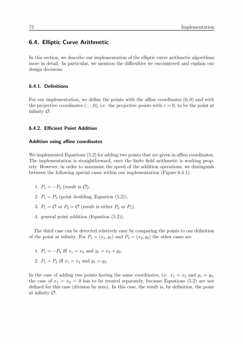
72 Implementation
6.4. Elliptic Curve Arithmetic
In this section, we describe our implementation of the elliptic curve arithmetic algorithmsmore in detail. In particular, we mention the difficulties we encountered and explain ourdesign decisions.
6.4.1. Definitions
For our implementation, we define the points with the affine coordinates (0, 0) and withthe projective coordinates (·, ·, 0), i.e. the projective points with z = 0, to be the point atinfinity O.
6.4.2. Efficient Point Addition
Addition using affine coordinates
We implemented Equations (5.2) for adding two points that are given in affine coordinates.The implementation is straightforward, once the finite field arithmetic is working prop-erly. However, in order to maximize the speed of the addition operations, we distinguishbetween the following special cases within our implementation (Figure 6.4.1):
1. P1 = −P2 (result is O),
2. P1 = P2 (point doubling, Equation (5.2)),
3. P1 = O or P2 = O (result is either P2 or P1),
4. general point addition (Equation (5.2)).
The third case can be detected relatively easy by comparing the points to our definitionof the point at infinity. For P1 = (x1, y1) and P2 = (x2, y2) the other cases are
1. P1 = −P2 iff x1 = x2 and y1 = x2 + y2,
2. P1 = P2 iff x1 = x2 and y1 = y2.
In the case of adding two points having the same coordinates, i.e. x1 = x2 and y1 = y2,the case of x1 = x2 = 0 has to be treated separately, because Equations (5.2) are notdefined for this case (division by zero). In this case, the result is, by definition, the pointat infinity O.

6.4 Elliptic Curve Arithmetic 73
Figure 6.4.1 Flow diagram of the decision process to distinguish the special cases forpoint addition in affine coordinates.
P1 = or
P2 =
x1 = x2
y1 + y2 = x1
y1 = y2
x1 = 0
true false
true false
falsetrue
falsetrue
true false
P1 = -P2
P1 = P2
Return P1 + P2
Return 2P1
Return P2 or P1
Return
Addition using mixed coordinates
Analogue to the addition using affine coordinates, adding a point given in affine coordi-nates to a point given in projective coordinates can be realized by simply implementingEquations (5.4). We also distinguish the special cases mentioned above (Figure 6.4.2).Due to the representation in different coordinates, the conditions for these special caseshave to be slightly modified. Suppose we are given a point Pproj = (X1, Y1, Z1) given inprojective coordinates and a point Paff = (x2, y2) given in affine coordinates. TransferringPproj to affine coordinates, we get Pproj = (X1/Z1, Y1/Z
21). Now, we can use the conditions
for points in affine coordinates to derive the special cases for mixed coordinates.
These cases are
1. Pproj = −Paff iff X1 = x2 · Z1 and Y1 = (x2 + y2) · Z21 ,
2. Pproj = Paff iff X1 = x2 · Z1 and Y1 = y2 · Z21 .

74 Implementation
Figure 6.4.2 Flow diagram of the decision process to distinguish the special cases forpoint addition in mixed coordinates.
Paff = or
Pproj =
X1 = x2 · Z1
Y1 = y2 · Z12
Y1 = (x2 + y2) · Z12
true false
true false
falsetrue
falsetrue
P1 = P2
P1 = -P2
Return P1 + P2
Return Pproj or Paff
Return
Return 2P1
6.4.3. Efficient Point Multiplication
Most of our implementation of the point multiplication methods has already been de-scribed in Chapter 5. However, since our sources do not explicitly cover the implemen-tation of the precomputation steps needed for the windowed methods, we present ourapproaches in the following.
Fixed-base comb method
The very fast scalar point multiplication of the fixed-base comb method (Algorithm 5.3.5)is due to the fact that a great part of the computation is done only once for a basepoint of the elliptic curve and stored for the actual computation. In our implemen-tation, the precomputation is done during the initialization step within the functionecdsaInitDomain(). This way, no further precomputation is necessary for the actualcomputation of scalar multiplications. The precomputation is done according to Algo-rithm 6.4.1.

6.4 Elliptic Curve Arithmetic 75
Algorithm 6.4.1 Precomputation steps for the Fixed-base comb method for point mul-tiplication
INPUT: Window width w, P ∈ E(GF (2m)).OUTPUT: Pn =
∑w−1i=0 ni2
i·dP for 0 ≤ n ≤ 2w − 1.
1: P0 ←− O.2: P1 ←− P .3: j ←− 2.4: while j ≤ 2w−1 do5: Pj ←− 2dPj�1.6: for r = 1 to j − 1 do7: Pj+r ←− Pj + Pr.8: j ←− j � 1.9: return Pn for 0 ≤ n ≤ 2w − 1
The computation in Step 5 equals to d doublings of the point Pj�1. Since doubling inprojective coordinates is faster than in affine coordinates, we convert the point to projec-tive coordinates before the computation and convert the result back to affine coordinatesafter the computation. The point addition in Step 7 is performed in affine coordinates,because the main multiplication routine needs the precomputed points given in affinecoordinates.
Window TNAF method
The TNAF method and the window TNAF method for point multiplication on Koblitzcurves require some amount of precomputation if several different curves shall be sup-ported. Our implementation contains a function ecpointInitKoblitzCurve() that iscalled within the initialization function ecdsaInitDomain() if the chosen curve is aKoblitz curve. This function essentially allocates the required dynamic memory andcomputes the following quantities needed for the
� Partial Modular Reduction (Algorithm 5.4.2) [59]:
– Vm,
– si = (−1)i
f(1− µUm+3−a−i) for i ∈ {0, 1}.
� Computation of TNAFw(ρ) (Algorithm 5.4.4) [59]:
– Uw,
– tw = 2Uw−1U−1w (mod 2w).

76 Implementation
� Window TNAF method (Algorithm 5.4.5) [59]:
– Ui for 0 < i < w,
– τ i = Uiτ − 2Ui−1 for 0 < i < w,
– αu and TNAF(αu) using Algorithm 6.4.2.
In above equations, Uk and Vk are the Lucas sequences that can be computed via the re-cursion formulas (Equation (5.12)), w is the window width for the window TNAF method,m is the extension degree of the finite field F2m, f is the cofactor and a is the parameterof the Koblitz curve Ea (see also Table 5.4.1).
Algorithm 6.4.2 Computation of αu and TNAF(αu)
INPUT: Window width wOUTPUT: αu,
(
k(u)w−1, k
(u)w−2, . . . , k
(u)0
)
= TNAF(αu) for u ∈ {1, 3, . . . , 2w−1−1}.1: α0 ←− 1.2: for i = 1 to 2w−2 do3: κ←− 2i + 1 partmod ((τm − 1)/(τ − 1)).
4:
(
k(2i+1)w−1 , k
(2i+1)w−2 , . . . , k
(2i+1)0
)
←− TNAF(κ).
5: α2i+1 ←− 0.6: for j = w − 1 downto 0 do7: α2i+1 ←− α2i+1 + k
(2i+1)j · τ j.
8: return αu and(
k(u)w−1, k
(u)w−2, . . . , k
(u)0
)
for u ∈ {1, 3, . . . , 2w−1 − 1}.
The window TNAF method (Algorithm 5.4.5) requires the precomputation of Pu = αuPfor u ∈ {1, 3, . . . , 2w−1 − 1}. In our implementation, we realize this precomputation withAlgorithm 6.4.3.
Algorithm 6.4.3 Precomputation steps for the window TNAF method for point multi-plication
INPUT: Window width w, P ∈ E(GF (2m)), (k(l)w−1, k
(l)w−2, . . . , k
(l)0 ) = TNAF(α2l+1) for
l ∈ {0, 1, . . . , 2w−2 − 1}OUTPUT: Pu = αuPu for u ∈ {1, 3, . . . , 2w−1 − 1}.1: for l = 0 to 2w−2 − 1 do2: Pl ←− O.3: for j = w − 1 downto 0 do4: if kj 6= 0 then5: if kj = 1 then6: P2l+1 ←− P2l+1 + τ jP .7: else

6.4 Elliptic Curve Arithmetic 77
8: P2l+1 ←− P2l+1 − τ jP .9: return Pu for u ∈ {1, 3, . . . , 2w−1 − 1}.
6.4.4. Timings
Table 6.4.1 Execution times in microseconds for point arithmetic on the elliptic curvesect163k1 which is a Koblitz curve over F2163 . Times were obtained on a Sharp Zaurusat 206MHz and on an Intel Pentium II at 300 MHz.
Arithmetic Operation Sharp Zaurus Intel Pentium II206 MHz 300 MHz
Point Addition (mixed coordinates) 121 � s 64 � sPoint Addition (affine coordinates) 158 � s 83 � sPoint Doubling 61 � s 35 � sPoint Multiplication Methods for General CurvesBinary Method 13560 � s 7440 � sWindow NAF Method (w = 4) 10920 � s 6000 � sMontgomery Method 8960 � s 4840 � sFixed-Base Comb Method (w = 9), withoutprecomputation time
2680 � s 1400 � s
Point Multiplication Methods for Koblitz CurvesTNAF Method 6720 � s 3080 � sWindow TNAF Method (w = 4) 5320 � s 2400 � sFixed-base Window TNAF Method (w = 11),without precomputation time
3160 � s 1440 � s
Table 6.4.1 reflects the execution times of point addition and multiplication on our targetplatform. The window sizes for the windowed multiplication methods correspond to thechoices that will be discussed in Section 6.5. The performance gap between addition inaffine and in mixed coordinates turns out to be greater than estimated in Section 5.3.1.The remaining times are better than our estimations. Table 6.4.2 shows the influenceof different window sizes on the execution times of the fixed-base point multiplicationmethods. Note, that our implementation also supports curves other than the 163-bitKoblitz curve used in the tables. However, since the results for other curves show a similarbehavior, we limit our presentation to the exemplary timings for the 163-bit Koblitz curve.

78 Implementation
Table 6.4.2 Execution times in milliseconds of fixed-base point multiplication methodsfor different window sizes on the elliptic curve sect163k1 which is a Koblitz curve overF2163 . Times were obtained on a Sharp Zaurus at 206MHz.
Window Fixed-base Comb Method Fixed-base Window TNAF MethodWidth Precomputation Multiplication Precomputation Multiplication
4 0.5ms 4.8ms5 1.5ms 4.4ms6 21.7ms 3.8ms 3.8ms 4.0ms7 32.4ms 3.2ms 9.5ms 3.8ms8 53.2ms 2.9ms 22.6ms 3.6ms9 94.8ms 2.7ms 52.6ms 3.4ms10 176.8ms 2.4ms 119.8ms 3.3ms11 240.1ms 2.2ms 268.6ms 3.2ms12 664.0ms 2.1ms 598.9ms 3.1ms
6.5. Implementation of the Elliptic Curve Digital SignatureAlgorithm (ECDSA)
Although the realization of the ECDSA according to Algorithms 3.3.2 (signature gen-eration) and 3.3.3 (signature verification) is straightforward, it involves several designdecisions, which we describe in this section. We explain which multiplication methodswe chose and which parameter settings lead to the best performance. After introducingthe flexible and modular structure of our implementation, we end this section with anelaboration on how strong random numbers for the ECDSA are obtained.
6.5.1. Optimal Point Multiplication Methods
Taking a look at Algorithms 3.3.2 and 3.3.3, one notices that the crucial operationsare the scalar point multiplication kG in the first algorithm and the two scalar pointmultiplications u1G and u2Q in the later one. They are crucial, because they dominate theexecution time of the algorithms. All other operations such as modular integer arithmetictake only a fraction of the time that scalar point multiplication on an elliptic curve takes.
The algorithms use two different types of scalar point multiplication:
1. multiplication of some scalar k with the fixed base point G
2. multiplication of some scalar l with an arbitrary point Q

6.5 ECDSA Implementation 79
For the first type of multiplication, we know the point G already during the initializationphase of our program. This point is declared together with the other domain parametersof the elliptic curve. Obviously, it would be advantageous to use a point multiplicationmethod that provides very fast execution times for the actual multiplication while takingpossibly longer to do the necessary precomputation. We have implemented two suchmultiplication methods, the fixed-base comb method (Algorithm 5.3.5) for general binarycurves and the fixed-base window TNAF method (Algorithm 5.4.5) for Koblitz curves.
Figure 6.5.1 Execution times and precomputation times of different fixed-point multi-plication methods on the Sharp Zaurus (163-bit Koblitz curve).
0
1
2
3
4
5
6
32 64 128 256 512 1024 2048 4096
Exe
cutio
n Ti
me
for M
ultip
licat
ion
[ms]
Number of Precomputed Points
Fixed-base Comb MethodFixed-base Window TNAF Method
0
100
200
300
400
500
600
32 64 128 256 512 1024 2048 4096
Exe
cutio
n Ti
me
for P
reco
mpu
tatio
n [m
s]
Number of Precomputed Points
Fixed-base Comb MethodFixed-base Window TNAF Method
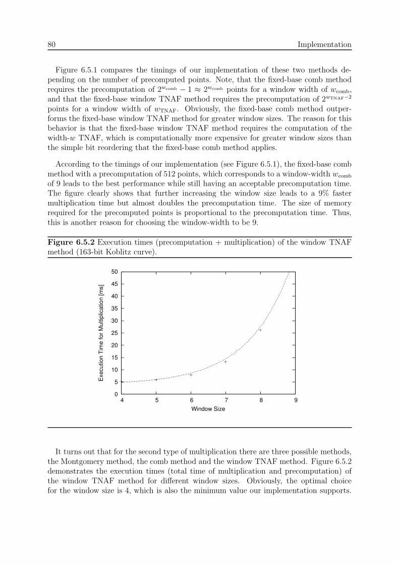
80 Implementation
Figure 6.5.1 compares the timings of our implementation of these two methods de-pending on the number of precomputed points. Note, that the fixed-base comb methodrequires the precomputation of 2wcomb − 1 ≈ 2wcomb points for a window width of wcomb,and that the fixed-base window TNAF method requires the precomputation of 2wTNAF−2
points for a window width of wTNAF. Obviously, the fixed-base comb method outper-forms the fixed-base window TNAF method for greater window sizes. The reason for thisbehavior is that the fixed-base window TNAF method requires the computation of thewidth-w TNAF, which is computationally more expensive for greater window sizes thanthe simple bit reordering that the fixed-base comb method applies.
According to the timings of our implementation (see Figure 6.5.1), the fixed-base combmethod with a precomputation of 512 points, which corresponds to a window-width wcomb
of 9 leads to the best performance while still having an acceptable precomputation time.The figure clearly shows that further increasing the window size leads to a 9% fastermultiplication time but almost doubles the precomputation time. The size of memoryrequired for the precomputed points is proportional to the precomputation time. Thus,this is another reason for choosing the window-width to be 9.
Figure 6.5.2 Execution times (precomputation + multiplication) of the window TNAFmethod (163-bit Koblitz curve).
0
5
10
15
20
25
30
35
40
45
50
4 5 6 7 8 9
Exe
cutio
n Ti
me
for M
ultip
licat
ion
[ms]
Window Size
It turns out that for the second type of multiplication there are three possible methods,the Montgomery method, the comb method and the window TNAF method. Figure 6.5.2demonstrates the execution times (total time of multiplication and precomputation) ofthe window TNAF method for different window sizes. Obviously, the optimal choicefor the window size is 4, which is also the minimum value our implementation supports.

6.5 ECDSA Implementation 81
Finally, Table 6.5.1 gives an overview of the execution times of the window TNAF method,the Montgomery method and the comb method. These values suggest that the windowTNAF method with a window-width of 4 is the best choice for Koblitz curves and theMontgomery method is the best choice for arbitrary curves.
Table 6.5.1 Execution times of different multiplication methods for arbitrary points onSharp Zaurus (163-bit Koblitz curve).
MethodExecution Time
(for precomputation andmain computation)
Window TNAF (w = 4) 5.32 msMontgomery 8.96 ms
Comb (w = 2) 13.68 ms
Finally, we should mention that there is also a method called Shamir’s trick [19] forsimultaneously computing two point multiplications as they are necessary for the ECDSAverify operation (Algorithm 6.5.1). However, the performance of this method turns outto be worse than doing two multiplications and one addition using the methods discussedabove (see Table 6.5.2).
Algorithm 6.5.1 Simultaneous point multiplication (Shamir’s trick) [19]
INPUT: Window width w, k = (ks−1, . . . , k1, k0)2, l = (ls−1, . . . , l1, l0)2, P , Q.OUTPUT: kP + lQ.
1: Compute iP + jQ for all i, j ∈ [0, 2w − 1].2: Write k = (kd−1, . . . , k1, k0) and l = (ld−1, . . . , l1, l0) where each ki and li is a bitstring
of length w, and d = dt/we.3: R←− O.4: for i = d− 1 downto 0 do5: R←− 2wR.6: R←− R + (kip + liQ).7: return R.

82 Implementation
Table 6.5.2 Execution times of verify operation with Shamir’s trick on Sharp Zaurus(163-bit Koblitz curve).
Window Width Execution Timewithout Shamir’s trick 11.64 ms
w = 2 25.96 msw = 3 23.26 msw = 4 22.38 msw = 5 23.42 msw = 6 27.10 ms
Table 6.5.3 summarizes which multiplication methods we chose for which case togetherwith the optimal window sizes.
Table 6.5.3 Overview of the used multiplication methods
General Curves Koblitz Curves
Arbitrary Point Montgomery Method Window TNAF method (w = 4)Fixed Point Fixed-base Comb Method (w = 9)
6.5.2. Modular Architecture
In order to offer the chance to use different multiplication methods for different types ofcurves, we organize the ECDSA layer of our implementation in a modular way. This isdone with a structure of type ecdsaDomain that is initialized during run-time with valuestailored to the elliptic curve to be used. Here is how this structure looks like:
typedef struct
{
EllipticCurvePoint G;
gf2mShortElement n;
gf2mLongElement mu;
EllipticCurve *curve;
// Precomputed Points
EllipticCurvePoint *FixedBasePrecomputedPoints;
EllipticCurvePoint *SimultaneousPrecomputedPoints;
// Function pointers to the arithmetic methods to be used

6.6 Integration into OpenSSL 83
void (*ecpointMultArbitrary)();
void (*ecpointMultGenerator)();
void (*ecpointMultSimultaneous)();
} ecdsaDomain;
It contains some elliptic curve domain parameters, the precomputed value mu that isused for long integer modular reduction (see Section 6.3.2 for details), two arrays ofprecomputed points for the multiplication methods that use precomputation and threefunction pointers. In the function ecdsaInitDomain(), these function pointers are setto point to the optimal multiplication methods depending on the type of elliptic curveas discussed above. The precomputation for these methods is done in the initializationfunction. The memory for the arrays of precomputed points is allocated dynamically. Weprovide the function ecdsaFreeDomain() to free the allocated memory.
6.5.3. Random Number Generation
The signature generation and certainly the key generation according to ECDSA requirethe generation of random numbers. These random numbers must be strong, i.e. anattacker should not be able to predict the random number or parts of it. Otherwise thesignature system would be vulnerable to attacks as described in [26]. Since the OpenSSLlibrary already contains a well-designed random number generator, we use the outputof the OpenSSL function RAND_bytes() for our random numbers. To ensure that theobtained number is not greater than the modulus n, we perform a modular reductionstep.
6.6. Integration into OpenSSL
For the integration into OpenSSL we used the following OpenSSL struct, which is definedin the file openssl/ec.h:
typedef struct ecdsa_method
{
const char *name;
ECDSA_SIG *(*ecdsa_do_sign)(const unsigned char *dgst, int dgst_len,
EC_KEY *eckey);
int (*ecdsa_sign_setup)(EC_KEY *eckey, BN_CTX *ctx, BIGNUM **kinv,
BIGNUM **r);
int (*ecdsa_do_verify)(const unsigned char *dgst, int dgst_len,
ECDSA_SIG *sig, EC_KEY *eckey);
int flags;
char *app_data;
} ECDSA_METHOD;

84 Implementation
Our implementation of this struct as well as the interface functions can be found in thefile openssl_interface.c. Here is how it looks like:
static ECDSA_METHOD rubcosy_ecdsa_meth = {
"RubCoSy ECDSA method",
rubcosy_ecdsa_do_sign,
rubcosy_ecdsa_sign_setup,
rubcosy_ecdsa_do_verify,
0, /* flags */
NULL /* app_data */
};
The declarations of the functions we implemented are in the file ecdsa.h. We implementedour own version of the ecdsa_do_sign()-method, the ecdsa_sign_setup()-method, andthe ecdsa_do_verify()-method. The implementation basically converts the OpenSSLtypes EC_KEY, BIGNUM, and ECDSA_SIG to the corresponding lightweight types of ourECDSA implementation and calls the corresponding functions of our implementation.It also calls the initialization routines whenever necessary.
Figure 6.6.1 Call Graph for the ECDSA do sign()-method.
ECDSA_do_sign()
ECDSA_OpenSSL() -> ecdsa_do_sign()
ECDSA_RubCoSy() -> ecdsa_do_sign()
rubcosy_check_domain()
rubcosy_domain_init()
ECDSA_sign_setup()
ecdsaSign_do()
ecdsaFreeDomain()
ecdsaInitDomain()
Part of our implementation (OpenSSL Interface Layer)Part of our implementation (ECDSA Layer)Part of the OpenSSL implementationPart of the OpenSSL implementation (not invoked)
Call OpenSSL routines in case of unsupported curves
Figure 6.6.1 illustrates what happens when the OpenSSL framework invokes the ECDSAsignature generation. The OpenSSL function ECDSA_do_sign() calls the member func-tion ecdsa_do_sign() of the ECDSA_METHOD-struct. If we replace the default struct with

6.6 Integration into OpenSSL 85
our implementation, our version of the ecdsa_do_sign()-function is invoked. Then, thefunctions rubcosy_check_domain() and rubcosy_domain_init() check whether our im-plementation supports the requested elliptic curve. If not, the corresponding memberfunction of the standard OpenSSL method struct is invoked. However, in case we dosupport the elliptic curve, the domain parameters are initialized (i.e. dynamic mem-ory is allocated, precomputation is done). Then, our implementation behaves similarto OpenSSL and first calls the OpenSSL function ECDSA_sign_setup(), followed by theecdsaSign_do()-method, which is part of our ECDSA Sign and Verify Layer.
Figure 6.6.2 Call Graph for the ECDSA sign setup()-method.
ECDSA_sign_setup()
ECDSA_OpenSSL() -> ecdsa_sign_setup()
ECDSA_RubCoSy() -> rubcosy_ecdsa_sign_setup()
rubcosy_check_domain()
rubcosy_domain_init()
ecdsaSign_setup()
ecdsaFreeDomain()
ecdsaInitDomain()
Part of our implementation (OpenSSL Interface Layer)Part of our implementation (ECDSA Layer)Part of the OpenSSL implementationPart of the OpenSSL implementation (not invoked)
Call OpenSSL routines in case of unsupported curves
The OpenSSL function ECDSA_sign_setup() behaves similar to ECDSA_do_sign()
(Figure 6.6.2) and calls, in case the elliptic curve is supported, the ecdsaSign_verify()-method, which is again part of our ECDSA Sign and Verify Layer.
Finally, Figure 6.6.3 describes which functions are called when the OpenSSL frame-work performs a signature verification. The actual verification is done using ourecdsaVerify()-method.
How can a program tell OpenSSL to use our optimized algorithms instead of theOpenSSL algorithms? We provide the function ECDSA_RubCoSy() which returns a pointerto the ECDSA_METHOD struct mentioned before. This pointer can be passed to the OpenSSLfunction void ECDSA_set_default_method(const ECDSA_METHOD *) in order to informthe OpenSSL framework that our optimized implementation shall be used instead of theOpenSSL implementation. This can be done in the global initialization section of the

86 Implementation
program. The function rubcosy_domain_free() should be called in the global finaliza-tion section of the program in order to free all memory dynamically allocated by ourimplementation.
Figure 6.6.3 Call Graph for the ECDSA do verify()-method.
ECDSA_do_verify()
ECDSA_OpenSSL() -> ecdsa_do_verify()
ECDSA_RubCoSy() -> rubcosy_ecdsa_do_verify()
rubcosy_check_domain()
rubcosy_domain_init()
ecdsaVerify()
ecdsaFreeDomain()
ecdsaInitDomain()
Part of our implementation (OpenSSL Interface Layer)Part of our implementation (ECDSA Layer)Part of the OpenSSL implementationPart of the OpenSSL implementation (not invoked)
Call OpenSSL routines in case of unsupported curves
6.7. Optimizations
To increase the performance of our implementation, we primarily tried three differentoptimization methods. Of course, we also paid attention to producing efficient and low-overhead code throughout the whole implementation. However, we expected the threeapproaches
� inline functions
� loop unrolling
� inline assembler
to significantly increase the execution speed of our verify and sign operations. In thischapter we describe these three approaches in detail. Additionally, we present our auto-matic source code generator, which enables us to generate source code that is tailored tospecific elliptic curves with specific key sizes. Hence, our implementation is not tied toone particular curve but can be configured to support any binary curve without loss ofperformance.

6.7 Optimizations 87
6.7.1. Inline Functions
Inline functions are an extension to the C programming language and allow the program-mer to direct the compiler to integrate the function’s code into the code of its callers.This eliminates the function-call overhead and might also improve the performance ofthe compiler-optimized code. The trade-off is, however, that the object code may be-come larger. Actually, the only difference to the conventional macro method which uses#define-statements to replace normal functions is that the type checking during com-pilation is not disabled. Furthermore, debugging the code is much easier, because theinlining can be disabled with a compiler switch leading to normal function code.
In our implementation, source files with the term inline within their filename containthe source code for inline functions. It was necessary to put them into separate files,because the compiler needs to see their source while compiling the source of the callers,i.e. the source of the inline functions has to be included in all source files that containfunctions that call these inline functions.
The typical functions that we declared as inline functions are utility functions, e.g.functions that assign the coordinates of a point to another point or functions that comparethe absolute values of two long integers. Nevertheless, using our automatic source codegeneration tool, we could compare the speed of a number of combinations and choose theoptimal combination (see also Section 6.7.4).
6.7.2. Loop Unrolling
The largest gain in performance can be achieved with so-called loop unrolling. With thismethod, loops in the source code like
for (i = 0; i < 10; i++)
foo[i] = 0;
are unrolled, i.e. their code is written as
foo[0] = 0;
foo[1] = 0;
foo[2] = 0;
foo[3] = 0;
...
foo[9] = 0;
In modern processors with pipeline architecture short loops significantly deteriorate theexecution speed. The reason for this is that a loop is essentially a number of instructions

88 Implementation
and a conditional branch instruction at the end. The conditional branch evaluates an ex-pression that changes within the loop body. In our example above, the branch instructionchecks whether the variable i is less than 10 after each loop cycle. In a pipeline archi-tecture the processor cannot load the next instruction into the pipeline as long as theexpression is not evaluated, because it does not know which will be the next instruction(the first instruction of the loop or the instruction following the loop).
Imagine, for example, we have a 4-stage pipeline with the following stages:
1. Fetch (F):The next instruction is fetched from the instruction buffer.
2. Decode (D):The instruction is decoded, i.e. the processor examines which operands will beneeded and what shall be done with them.
3. Execute (E):The processor executes the instruction, e.g. adds two operands.
4. Write back (W):The result of the execution step is written to the register file and is now availablefor following instructions.
The CPU instructions implementing the loop above written in pseudocode might be
0: foo[i] = 0;
1: i = i + 1;
2: if (i < 10) goto 0;
3: ...
4: ...
As Figure 6.7.1 illustrates, the conditional jump in instruction 2 cannot be executedbefore the result of instruction 1 is written back to the register file. Moreover, it dependson the result of instruction 2 whether instruction 3 or instruction 0 is executed next.Hence, instruction 0 will be fetched after instruction 2 is executed and two holes (NOP-operations) are inserted into the pipeline.
Unrolling the loops reduces the number of branch instructions within the code, sothat the pipeline can be filled continuously with instructions. Hence, the instructionthroughput and therefore the execution speed of the operations rises.

6.7 Optimizations 89
Figure 6.7.1 Stalled pipeline, because the result of a previous instruction is not availableon time.
F D E W
2 1 03
2 13
34 2
0 2
Instruction 2 cannot be executed, because the new value for i is not available yet
After executing instruction 2, the pipeline is flushed and the correct instruction 0 is fetched.
Instruction 3 and 4 enter the pipeline as long as instruction 2 is not evaluated
In our case, unrolling the loops more than doubled the execution speed of the signatureand verify operations. However, we did not unroll every loop. For example, in the algo-rithm for multiplying two elements of F2m (Algorithm 6.3.1), there are two nested loops(Steps 3 and 4). It turns out, that unrolling the inner loop leads to an 18% performancegain whereas unrolling both loops deteriorates the performance. For this reason, we usedour automatic source code generation utility to determine the level of unrolling that leadsto the best overall performance.
Together with the inline functions, the loop unrolling optimizations sped up the execu-tion of the Montgomery point multiplication method from originally 25.2ms on the SharpZaurus to 8.96ms. This is equivalent to an acceleration factor of 2.8. This demonstratesthe significance of this optimization method.
6.7.3. Inline Assembler
The compiler we utilized, the Gnu GCC compiler, supports so-called inline assemblerstatements, which embed assembler statements directly in the source code. This enablesthe programmer to directly access native processor commands that are not supportedby the C programming language, e.g. bit shift operations or add-with-carry operations.Additionally the programmer has direct control over the compiler output and may hand-optimize the order of instruction execution.
Figure 6.7.2 Multi-word bitwise right shift.
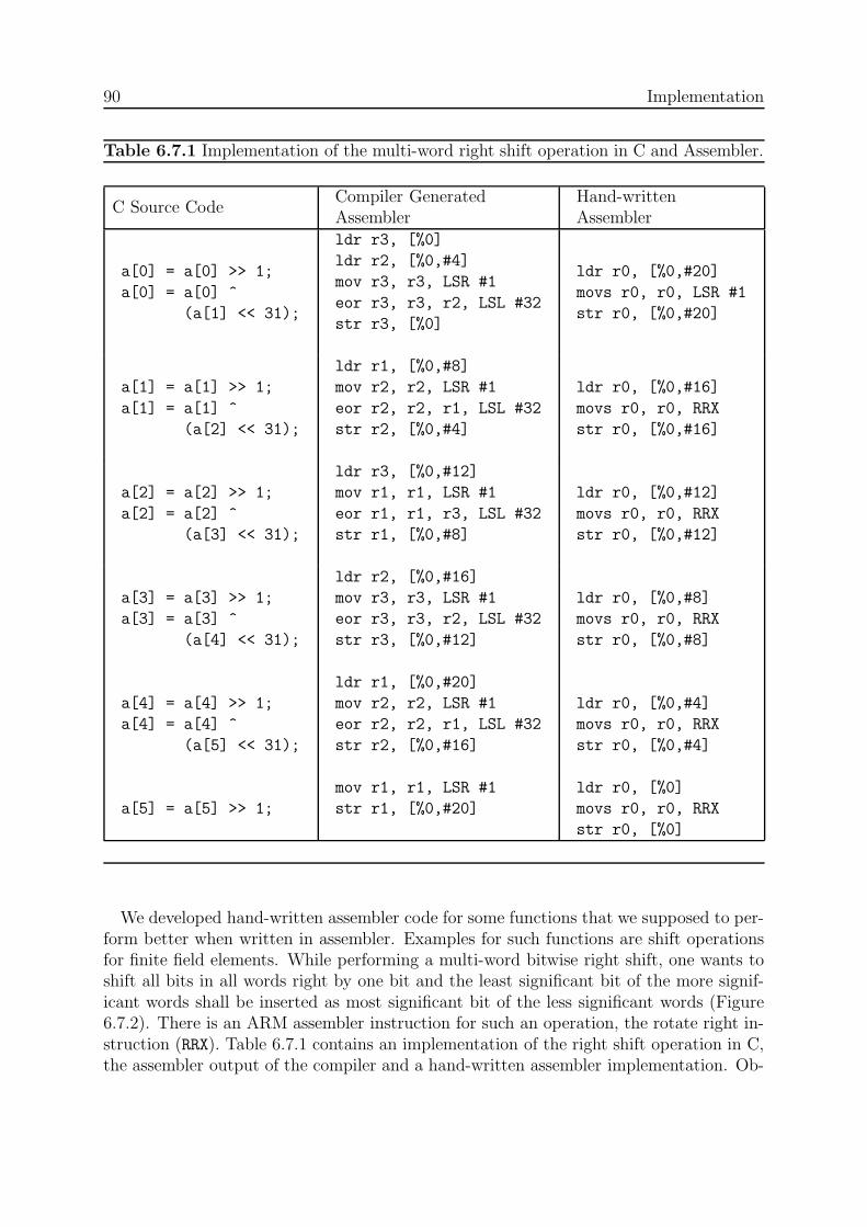
90 Implementation
Table 6.7.1 Implementation of the multi-word right shift operation in C and Assembler.
C Source CodeCompiler GeneratedAssembler
Hand-writtenAssembler
a[0] = a[0] >> 1;
a[0] = a[0] ^
(a[1] << 31);
ldr r3, [%0]
ldr r2, [%0,#4]
mov r3, r3, LSR #1
eor r3, r3, r2, LSL #32
str r3, [%0]
ldr r0, [%0,#20]
movs r0, r0, LSR #1
str r0, [%0,#20]
a[1] = a[1] >> 1;
a[1] = a[1] ^
(a[2] << 31);
ldr r1, [%0,#8]
mov r2, r2, LSR #1
eor r2, r2, r1, LSL #32
str r2, [%0,#4]
ldr r0, [%0,#16]
movs r0, r0, RRX
str r0, [%0,#16]
a[2] = a[2] >> 1;
a[2] = a[2] ^
(a[3] << 31);
ldr r3, [%0,#12]
mov r1, r1, LSR #1
eor r1, r1, r3, LSL #32
str r1, [%0,#8]
ldr r0, [%0,#12]
movs r0, r0, RRX
str r0, [%0,#12]
a[3] = a[3] >> 1;
a[3] = a[3] ^
(a[4] << 31);
ldr r2, [%0,#16]
mov r3, r3, LSR #1
eor r3, r3, r2, LSL #32
str r3, [%0,#12]
ldr r0, [%0,#8]
movs r0, r0, RRX
str r0, [%0,#8]
a[4] = a[4] >> 1;
a[4] = a[4] ^
(a[5] << 31);
ldr r1, [%0,#20]
mov r2, r2, LSR #1
eor r2, r2, r1, LSL #32
str r2, [%0,#16]
ldr r0, [%0,#4]
movs r0, r0, RRX
str r0, [%0,#4]
a[5] = a[5] >> 1;
mov r1, r1, LSR #1
str r1, [%0,#20]
ldr r0, [%0]
movs r0, r0, RRX
str r0, [%0]
We developed hand-written assembler code for some functions that we supposed to per-form better when written in assembler. Examples for such functions are shift operationsfor finite field elements. While performing a multi-word bitwise right shift, one wants toshift all bits in all words right by one bit and the least significant bit of the more signif-icant words shall be inserted as most significant bit of the less significant words (Figure6.7.2). There is an ARM assembler instruction for such an operation, the rotate right in-struction (RRX). Table 6.7.1 contains an implementation of the right shift operation in C,the assembler output of the compiler and a hand-written assembler implementation. Ob-

6.7 Optimizations 91
viously, the compiler-generated code consists of 23 statements whereas the hand-writtencode consists of only 18 statements. Hence, we could theoretically increase the executionspeed by about 20%.
However, it turned out that the performance achieved by using native assembler in-structions for such operations is worse than the performance the compiler optimized codeachieves. The reason for this is that the compiler does a lot of code reordering, i.e. itchanges the order of execution of some statements, and thereby optimizes register us-age and memory access. Moreover, the compiler does not only consider the relativelyshort function that implements the shift operation, but also the longer function that callsthe shift function. Remember, we use inline functions, therefore the compiler looks atthe whole code including the replaced versions of the shift function during optimization.Unfortunately, using inline assembler prevents the compiler from performing such an opti-mization, because the hand-written assembler sections are included after the optimizationstage.
Hence, in order to further speed up the code, it would be necessary to hand-write largerparts of the code in assembler and hand-optimize register usage and memory access. Webelieve that the amount of time necessary to do this is not justified by the expected gainof speed and loss of portability. Consequently, our implementation does not use any inlineassembler.
6.7.4. Automatic Source Code Generator
The reasons for us to develop an automatic source code generator are essentially thefollowing:
� Loop unrolling for different key sizes cannot be done in C (for example, with#define-macros).
� Different target platforms or different curves might require different levels of loopunrolling or inline functions for maximum execution speed.
� The modular reduction algorithm in F2m (Algorithm 6.3.2) heavily depends on thereduction polynomial, which varies for different curves.
Our generator creates the source files gf2m_gen.h, gf2m_gen.c and gf2m_inline_gen.c.These files contain the definitions for the finite field arithmetic such as the reductionpolynomial to be used or the extension degree m. Moreover, all finite field arithmeticoperations are generated, since they contain loops that are unrolled. The generator alsocreates a version of the modular reduction algorithm (Algorithm 6.3.2) that is tailored toa specific reduction polynomial. The tool can be configured via command line options orvia the configuration file ecclib.conf. For more details about the usage of the generatorand the meaning of the parameters, we refer to Appendix A.1.2.
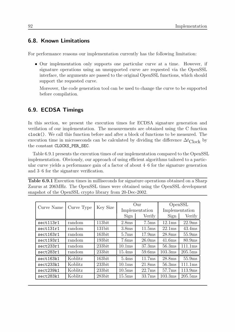
92 Implementation
6.8. Known Limitations
For performance reasons our implementation currently has the following limitation:
� Our implementation only supports one particular curve at a time. However, ifsignature operations using an unsupported curve are requested via the OpenSSLinterface, the arguments are passed to the original OpenSSL functions, which shouldsupport the requested curve.
Moreover, the code generation tool can be used to change the curve to be supportedbefore compilation.
6.9. ECDSA Timings
In this section, we present the execution times for ECDSA signature generation andverifation of our implementation. The measurements are obtained using the C functionclock(). We call this function before and after a block of functions to be measured. Theexecution time in microseconds can be calculated by dividing the difference ∆tClock bythe constant CLOCKS_PER_SEC.
Table 6.9.1 presents the execution times of our implementation compared to the OpenSSLimplementation. Obviously, our approach of using efficient algorithms tailored to a partic-ular curve yields a performance gain of a factor of about 4–6 for the signature generationand 3–6 for the signature verification.
Table 6.9.1 Execution times in milliseconds for signature operations obtained on a SharpZaurus at 206MHz. The OpenSSL times were obtained using the OpenSSL developmentsnapshot of the OpenSSL crypto library from 20-Dec-2002.
Curve Name Curve Type Key SizeOur
ImplementationOpenSSL
ImplementationSign Verify Sign Verify
sect113r1 random 113bit 2.8ms 7.5ms 12.1ms 22.9mssect131r1 random 131bit 3.8ms 11.5ms 22.1ms 43.4mssect163r1 random 163bit 5.7ms 17.9ms 28.8ms 55.9mssect193r1 random 193bit 7.6ms 26.0ms 41.6ms 80.9mssect233r1 random 233bit 10.1ms 37.3ms 56.3ms 111.1mssect283r1 random 233bit 15.4ms 59.6ms 103.3ms 205.5ms
sect163k1 Koblitz 163bit 5.4ms 11.7ms 28.8ms 55.9mssect233k1 Koblitz 233bit 10.1ms 21.8ms 56.3ms 111.1mssect239k1 Koblitz 233bit 10.5ms 22.7ms 57.7ms 113.9mssect283k1 Koblitz 283bit 15.5ms 33.7ms 103.3ms 205.5ms

Previous Work 93
7. Previous Work
In the past years since Miller and Koblitz proposed Elliptic Curve Cryptosystems variouspapers dealt with the efficient implementation of ECC on different platforms. In thissection, we present some of this work together with the execution times on differentplatforms.
In [54] the authors describe an efficient software implementation of elliptic curves thatis optimized for processors with 64-bit word size. The paper mentions a couple of usefultricks for an optimized implementation. The execution time for a scalar point multiplica-tion on an elliptic curve over F2155 is 124ms on a Sun SPARC IPC at 25MHz and 9.9mson a DEC Alpha 3000 at 175MHz.
An extensive study of software implementation of the NIST-recommended elliptic curvesover binary fields can be found in [19] by Hankerson, Hernandez and Menezes. We tookmost algorithms from this paper. The authors treat general elliptic curves over F2m as wellas Koblitz curves whose special structure can be exploited for faster arithmetic. Theyobtained the execution times for scalar point multiplications on a Pentium II 400MHzworkstation. See Table 7.0.2 for an overview of the results.
Table 7.0.2 Execution times for scalar point multiplication on a Pentium II at 400MHzusing different algorithms [19].
Underlying fieldF2163 F2233 F2283
Random CurvesBinary method (affine coordinates) 9.178 ms 21.891 ms 34.845 msBinary method 4.716 ms 10.775 ms 16.123 msBinary NAF method 4.002 ms 9.303 ms 13.896 msWindow NAF method with w = 4 3.440 ms 7.971 ms 11.997 msMontgomery method 3.240 ms 7.697 ms 11.602 msFixed-base comb method with w = 4 1.683 ms 3.966 ms 5.919 ms
Koblitz CurvesTNAF method 1.946 ms 4.349 ms 6.612 msWindow TNAF method with w = 5 1.442 ms 2.965 ms 4.351 msFixed-base window TNAF with w = 6 1.176 ms 2.243 ms 3.330 ms
Weimerskirch, Paar and Shantz implemented elliptic curves over binary fields on aPalmOS device with Motorola Dragonball CPU running at 16 MHz [64]. They chose the

94 Previous Work
NIST-recommended random curves and Koblitz curves over F2163 . The execution timesare summarized in Table 7.0.3.
Table 7.0.3 Execution times for scalar point multiplication on a Dragonball CPU at 16MHz using different algorithms [64]. The underlying field is F2163 .
Random CurvesAddition-subtraction method 3310 msSliding windows method (w = 4) 3070 msWidth-w addition-subtraction method 2960 msMontgomery method 2730 msFixed-base comb method with w = 4 1430 msFixed-base comb method with w = 8 790 ms
Koblitz CurvesTNAF method 1670 msWindow TNAF method with w = 4 1510 msWindow TNAF method with w = 5 1680 msFixed-base window TNAF with w = 6 1080 msFixed-base window TNAF with w = 10 870 ms
In September 2002, Sun Microsystems donated an elliptic curve implementation tothe OpenSSL project [3], a programming group that works on an open-source versionof the Secure Sockets Layer (SSL) encryption system. So far, the code is not optimizedfor particular platforms or elliptic curves. Currently the Montgomery method and theWindow NAF method are used for scalar point multiplication on curves over binary fields.In [18] execution times for the ECDSA sign and verify operation on a Yopy PDA withStrongARM CPU at 200 MHz and an Sun UltraTM-80 server equipped with a 450 MHzUltraSPARC II processor are presented. The execution times of the ECDSA sign andverify operations are summarized in Table 7.0.4.
Table 7.0.4 Execution times of ECDSA operations on a StrongARM CPU at 200 MHz(Yopy) and on an UltraSPARC II processor at 450 MHz.
Platform ECDSA-Operation 163-bit 193-bit
Ultra-80 Verify 6.8 ms 9.2 msSign 13.0 ms 18.1 ms
Yopy Verify 46.5 ms 76.6 msSign 24.5 ms 39.0 ms

Summary and Conclusions 95
8. Summary and Conclusions
In this thesis, we carefully analyzed the secure charging protocol with respect to theuse of different digital signature schemes. An important part of this analysis was therecommendation of key sizes to be used. Due to the micro payment character of thisapplication, we believe that key sizes below the commonly recommended 1024-bit RSAare possible. According to our examinations, the required level of security, which is that— with a financial effort proportionate to the expected gain of about 200
�— it should
not be possible to break the keys in less than 24 hours, can be achieved with 704-bitRSA keys (respectively, 131-bit ECDSA over binary curves) until the year 2006. Fora sufficient protection until the year 2015, we recommend larger RSA keys with a sizeof at least 1024 bits (respectively, 163-bit ECDSA over binary curves). Of course, theserecommendations must be treated with care, since we cannot fully anticipate the effects ofprogress in cryptanalysis. We therefore recommend to continuously monitor the progressin this area and to adapt the key sizes when necessary.
Having determined the required level of security, we evaluated the performance of theRSA signature scheme and the ECDSA signature scheme on the basis of the executiontimes on our target platform. We proposed a new measure that takes into account thespecial organization of state-of-the-art communication protocols such as the secure charg-ing protocol. In these protocols, a device has to perform signature verification, signaturegeneration or both — depending on its role in the communication process. As a result ofour examination we can say that signature schemes based on elliptical curves outperformclassical signature schemes such as RSA in particular for high levels of security. Withrespect to the required storage space and transmission bandwidth, ECC is clearly thebetter choice. Nevertheless, in some applications that predominantly require signatureverification or need only very low levels of security, RSA may still be a good choice —even for applications in the area of wireless communications.
We implemented digital signatures based on general elliptic curves over binary finitefields as well as Koblitz curves. During this process we implemented several different pointmultiplication methods and determined the optimal choice for our application and targetplatform. Using the fixed-base comb method for multiplying the base point of the curveand the Montgomery method for multiplying arbitrary points, a signature generation ona StrongARM CPU clocked at 206 MHz takes 5.7ms and a signature verification takes17.9ms for 163-bit ECDSA. In case of Koblitz curves, we use the window TNAF method,which enables us to verify a signature on a 163-bit Koblitz curve in 11.7ms. This is aspeed up of 500% compared to the current ECDSA implementation using curves over F2m
of the OpenSSL project.
Although our implementation supports only one particular curve during run-time, we

96 Summary and Conclusions
provided a tool that allows easy adaptation to different curves during compile time. Fi-nally, the integration into the OpenSSL framework allows easy reuse of the implementationin future communication protocols or other applications.
We integrated our ECDSA implementation into the prototype implementation of theSecure Charging Protocol, which is currently developed by Lamparter, Paul, and Westhoff.A test run of the protocol prototype showed that ping packets between different nodes of atest network could be successfully transmitted. Unfortunately, the current prototype doesnot allow any statistics about the network performance and especially the performance ofthe digital signature operations. Hence, an interesting objective for future work would beto examine the network performance and the computational load for the network nodescaused by the signature operations in a realistic network scenario.

Appendix 97
A. Appendix
A.1. Ecclib Manual
A.1.1. Configuration with eccdefs.h
The file eccdefs.h contains a number of #define’s which influence the behavior of theEcclib code:
� #define USE_OPENSSL_RNG
This #define should always be enabled, because it tells the compiler to use therandom number generator shipped with the OpenSSL library. If the #define isdisabled, simple calls to rand() are used to generate the random secrets needed forthe signature generation process.
� #define USE_OPENSSL_FOR_UNSUPPORTED_FIELD
This #define tells our implementation to call the OpenSSL default routines forsignature generation and verification if it does not support the requested curve.Remember that within OpenSSL the type of curve that shall be used for the signa-ture operations can be dynamically chosen, therefore it might be the case that ourimplementation has not been compiled for the requested curve.
� #define SKIP_DGST_LEN_CHECK
OpenSSL usually checks if the length of the digest of the message to be signed isgreater than the size of the key in bytes. This causes problems when the key size isless than 160-bits (20 bytes). By enabling this switch one can tell our implementa-tion to skip the check. This #define is also enabled by default.
� #define TEST_EXEC_TIME
This defines how the execution times of the self-test routines are obtained. If theswitch is enabled, the self-test routines do not check if the results of the operationsare correct, but only measure the execution times. The screen output is kept to aminimum in this mode. This #define is disabled by default.
� #define USE_MEMxxx_FUNCTIONS
This #define determines whether our implementation uses functions like memcpy()
or memset() or replaces them with loops. We did not notice any influence on theperformance, so the switch is disabled by default.
� #define AUTOSKIP_LEADING_ZEROS
This switch should always be disabled.

98 Appendix
� #define USE_SHAMIRS_TRICK
Enabling this switch tells the compiler to use Shamir’s trick (Algorithm 6.5.1) ofsimultaneous point multiplication for the signature verification. As stated in Section6.5.1, this deteriorates the overall performance, so this switch should always bedisabled.
A.1.2. Code Generator EcclibCodeGen and Configuration ecclib.conf
As mentioned in Section 6.7.4, EcclibCodeGen generates the source files gf2m_gen.h,gf2m_gen.c, and gf2m_inline_gen.c during the make process. The tool can be config-ured with the configuration file ecclib.conf.
The options within ecclib.conf are the following:
� CURVE=〈OpenSSL Curve Identifier String〉This option determines which elliptic curve is supported by our library. The string〈OpenSSL Curve Identifier String〉 is used within OpenSSL to denote the curve andcan be found in the OpenSSL header file openssl/obj_mac.h. Examples for suchstrings are sect113r1, sect113r2, sect131r1, sect131r2, sect163r1, sect163r2,sect163k1, sect193r1, sect193r2, sect233r1, and sect233k1. The names are thesame as the names of the curves standardized by SECG in [44]. Note, that onlycurves over F2m are supported.
� COMBWINDOW=〈wcomb〉This specifies the size of the window used for the fixed-base comb method for pointmultiplication (Algorithm 5.3.5). Note, that our implementation demands a lowerbound of wcomb ≥ 2.
� TNAFWINDOW=〈wTNAF〉The size of the window used for the window TNAF method (Algorithm 5.4.5) isdetermined by this option. Note, that our implementation demands a lower boundof wTNAF ≥ 4.
� SHAMIRWINDOW=〈wShamir〉Since we also implemented simultaneous point multiplication (Algorithm 6.5.1), thisoption determines the window size for this algorithm.
� MAKEINLINE=1111100111101101
This option determines which of the 16 automatically generated functions shall beinline functions and which not. Each digit corresponds to one function. A value of 1means that the function shall be generated as inline function and a value of 0 meansthat it shall be a normal function. Normally, these settings should not be changed,because they were determined with intensive tests. However, if the target platformdiffers from the original Zaurus PDA platform, changing this setting might improvethe performance.

A.1 Ecclib Manual 99
� UNROLLLEVEL=2222222122212222
Our source code generator can be configured to support different levels of loopunrolling. Each digit corresponds to one of the 16 automatically generated functions.The values determine whether
(0) functions like memcpy() shall be used,
(1) simple for-loops shall be used,
(2) most loops shall be unrolled,
(3) all loops shall be unrolled or
(4) assembler implementations shall be used.
Note, that not every function supports all options. Please consider the source codeof the generator for details. Normally, these settings should not be changed, becausethey were determined with intensive tests. However, if the target platform differsfrom the original Zaurus PDA platform, changing this setting might improve theperformance.
� HEADER=〈Filename〉Defines the name of the file that shall contain source code for the generated headerfile. The default filename is gf2m_gen.h.
� SOURCE=〈Filename〉Defines the name of the file that shall contain source code for the generated sourcefile. The default filename is gf2m_gen.c.
� INLINE=〈Filename〉Defines the name of the file that shall contain source code for the generated sourcefile containing the inline function. The default filename is gf2m_inline_gen.c.
Finally, note that the CURVE=〈OpenSSL Curve Identifier String〉 option can also bepassed via command line parameter. The code generator then uses the passed settingand updates the ecclib.conf file.
A.1.3. Self-Test-Routines
With make test the executable ecclib.out, which contains a number of self-test rou-tines, is built. Which self-test routines are executed can be determined in the source filemain.cpp. Here is a list of the tests available together with the corresponding #define:
� #define TEST_BASIC_ARITHMETIC
This test routine checks whether the finite field and long integer arithmetic workscorrectly. In particular, the finite field multiplication, addition and squaring ischecked. Moreover, the routine tests the elliptic curve point addition in affine andalso in mixed coordinates. The test determines whether elliptic curve point doublingworks properly. Finally, almost all long integer routines are checked.

100 Appendix
� #define TEST_POINT_MULTIPLICATION
This #define enables the elliptic curve point multiplication tests. All methodsthat are implemented are called with the same input parameters and checked forcorrectness. This routine also determines the execution times of the different pointmultiplication methods.
� #define TEST_ECCLIB_SIGNATURE
This test checks whether signature generation and signature verification works cor-rectly. The tests are performed on the ECDSA Sign and Verify Layer, hence, theOpenSSL interface is not involved. Consequently, the execution times obtained withthis test are slightly better due to the reduced overhead.
� #define TEST_OPENSSL_COMPATIBILITY
By enabling this #define, the compatibility of the signatures of our implementationto the OpenSSL signature routines is checked. This is done by generating a signaturewith our routines and verifying it with the OpenSSL routines. The test functionalso generates signatures with the OpenSSL routines and verifies them with ourroutines.
� #define TEST_OPENSSL_SIGNATURE
The integration into OpenSSL is checked with this test routine. Consequently, thesigning and verifying is performed by invoking the OpenSSL interface. In additionto this, the execution times are measured.
� #define TEST_COMPARE_RSA_VS_ECDSA
This test compares the execution times of our ECDSA implementation with theexecution times of the OpenSSL implementation of the RSA signature scheme. Thebit sizes of the keys are chosen so that both schemes provide a comparable level ofsecurity.
A.2. Manual of the Certificate Tool CertGen
The CertGen-Tool can be used to generate ECDSA keys and certificates. It supportsthree different functions:
1. Generate a self-signed certificate for the Certificate Authority (CA) containing theCA public key and a separate file that contains the CA private key
2. Generate a CA-signed certificate for a node containing the node’s public key and aseparate file that contains the node’s private key
3. Verify a certificate, i.e. check if the CA signature is valid and the certificate has notexpired
These functions use our ECDSA implementation for the signature generation and verifi-cation and the OpenSSL routines for the certificate handling.

A.2 Manual of the Certificate Tool CertGen 101
A.2.1. CA Certificate Generation
In order to generate a set of CA keys and a certificate, CertGen should be invoked withthe following command:
CertGen generate ca 〈ca-arguments〉
where 〈ca-arguments〉 includes the following mandatory parameters:
� ISSUER=〈name of the issuer of the certificate〉
� SUBJECT=〈name of the subject of the certificate〉
� SERIALNUMBER=〈serial-number of the certificate〉
� CA-CERTFILE=〈name of the file that shall contain the certificate to be created〉
� CA-KEYFILE=〈name of the file that shall contain the private key to be created〉
A.2.2. Node Certificate Generation
In order to generate a set of node keys and a certificate, CertGen should be invoked withthe following command:
CertGen generate node 〈node-arguments〉
where 〈node-arguments〉 includes the following mandatory parameters:
� ISSUER=〈name of the issuer of the certificate〉
� SUBJECT=〈name of the subject of the certificate〉
� SERIALNUMBER=〈serial-number of the certificate〉
� CA-KEYFILE=〈name of the file that contains the private key to sign the node certificate〉
� CERTFILE=〈name of the file that shall contain the node certificate to be created〉
� KEYFILE=〈name of the file that shall contain the private key to be generated〉

102 Appendix
A.2.3. Certificate Verification
In order to verify a certificate, CertGen should be invoked with the following command:
CertGen verify 〈verify-arguments〉
where 〈verify-arguments〉 includes the following mandatory parameters:
� CA-CERTFILE=〈file name of the CA certificate〉� CERTFILE=〈file name of the certificate to be verified〉
A.3. OpenSSL Command Line Parameters
We used OpenSSL to generate RSA keys and RSA certificates as well as RSA signatures.In this section, we shortly describe the necessary OpenSSL command line options.
A.3.1. Generate RSA private key file
The following command generates a file containing a private RSA key with a size of keysizebits:
openssl genrsa -out 〈keyfile〉 〈keysize〉
To convert the file keyfile to the ASN.1 distinguished encoding rules (DER), we used thefollowing command:
openssl rsa -outform DER -out 〈name of DER encoded file〉 < 〈keyfile〉
A.3.2. Generate RSA certificate
Once a private key has been generated, the following OpenSSL commands can be used togenerate a DER encoded certificate file with the name certfile:
openssl req -new -key 〈keyfile〉 -out 〈certificate request file〉openssl x509 -req -in 〈certificate request file〉 -signkey 〈keyfile〉
-out 〈certfile〉 -outform DER
A.3.3. Generate RSA signature
To generate a RSA signature of the input file infile using the private key stored in the filekeyfile and save it to the file sigfile, the following command can be used:
openssl rsautl -inkey 〈keyfile〉 -in 〈infile〉 -out 〈outfile〉 -raw

References 103
References
[1] Aodv. Available from http://moment.cs.ucsb.edu/AODV/aodv.html.
[2] Sharp zaurus - developer site.http://docs.zaurus.com/linux compiler setup howto.shtml.
[3] The openssl project, 1998–2000.For further information, see http://www.openssl.org.
[4] air-lan der wlan-zugang am flughafen munchen, March 2003. More information athttp://air-lan.munich-airport.de.
[5] ARM Limited. ARM Architecture Reference Manual, June 2000.
[6] I. Blake, G. Seroussi, and N. Smart. Elliptic Curves in Cryptography. CambridgeUniversity Press, 1999.
[7] M. Brown, D. Hankerson, J. L. Hernandez, and A. Menezes. Soft-ware implementation of the nist elliptic curves over prime fields. Lec-ture Notes in Computer Science, 2020:250–265, 2001. Available fromhttp://citeseer.nj.nec.com/brown01software.html.
[8] S. Buchegger and J.-Y. L. Boudec. The selfish node: Increasing routing security inmobile ad hoc networks. Technical Report RR 3354, IBM Research Report, 2001.
[9] S. Buchegger and J.-Y. L. Boudec. Performance analysis of the confidant proto-col: Cooperation of nodes - fairness in dynamic ad-hoc networks. In Proceedings ofIEEE/ACM Symposium on Mobile Ad Hoc Networking and Computing (MobiHOC),June 2002.
[10] S. Buchegger and J.-Y. Le Boudec. Nodes bearing grudges: Towards routing security,fairness, and robustness in mobile ad hoc networks. In Proceedings of the TenthEuromicro Workshop on Parallel, Distributed ad Network-based Processing, pages403–410. IEEE Computer Society, January 2002.
[11] L. Buttyan and J.-P. Hubaux. Enforcing service availability in mobile ad-hoc wans. InProceedings of IEEE/ACM Workshop on Mobile Ad Hoc Networking and Computing(Mobi-HOC), August 2000.
[12] L. Buttyan and J.-P. Hubaux. Stimulating cooperation in self-organizing mobile adhoc networks. Technical Report DSC/2001/046, EPFL-DI-ICA, August 2001.

104 References
[13] S. Das, C. E. Perkins, and E. M. Rover. Ad hoc on demand distance vector (aodv)routing. Internet-Draft, Mobile Ad-hoc Network (MANET) Working Group, IETF,October 1999.
[14] H. Deng, W. Li, and D. P. Agrawal. Routing security in wireless ad hoc networks.IEEE Communications Magazine, 40(10):70–75, October 2002.
[15] W. Diffie and M. E. Hellman. Multiuser cryptographic techniques. In Proceedings ofAFIPS National Computer Conference, pages 109–112, 1976.
[16] W. Diffie and M. E. Hellman. New directions in cryptography. IEEE Transactionson Information Theory, 22:644–654, 1976.
[17] T. ElGamal. A public key cryptosystems and a signature scheme based on discretelogarithms. In IEEE Transactions on Information Theory, 31, pages 469–472, 1985.
[18] V. Gupta, S. Gupta, S. Chang, and D. Stebila. Performance analysis of elliptic curvecryptography for ssl. In Proceedings of the ACM workshop on Wireless security, pages87–94. ACM Press, 2002.
[19] D. Hankerson, J. L. Hernandez, and A. Menezes. Software implementation of ellipticcurve cryptography over binary fields. Lecture Notes in Computer Science, 1965:1–24,2001. Available from http://citeseer.nj.nec.com/hankerson00software.html.
[20] heise online CeBIT special. Wlan-angebot von t-online, March 2003. Available fromhttp://www.heise.de/newsticker/data/uma-07.03.03-000/.
[21] Y. Hu, A. Perrig, and D. Johnson. Ariadne: A secure on-demand rout-ing protocol for ad hoc networks. In 8th ACM International Conferenceon Mobile Computing and Networking, September 2002. Available fromhttp://citeseer.nj.nec.com/hu02ariadne.html.
[22] J.-P. Hubaux, L. Buttyan, and S. Capkun. The quest for security in mobile ad hocnetworks. In Proceeding of the ACM Symposium on Mobile Ad Hoc Networking andComputing (MobiHOC), 2001.
[23] D. Johnson, D. A. Maltz, and J. Broch. The dynamic source routing protocol formobile ad hoc networks. Internet-Draft, Mobile Ad-hoc Network (MANET) WorkingGroup, IETF, October 1999.
[24] D. Johnson, A. Menezes, and S. Vanstone. The elliptic curve digital signature algo-rithm (ecdsa). A Certicom Whitepaper, 2001. Available from Certicom website athttp://www.certicom.com/resources/w papers/w papers.html.
[25] U. Jonsson, F. Alriksson, T. Larsson, P. Johansson, and G. Q. Maguire Jr. Mipmanet- mobile ip for mobile ad hoc networks. In MobiHoc 2000, 2000.

References 105
[26] J. Kelsey, B. Schneier, D. Wagner, and C. Hall. Cryptanalytic attacks on pseudoran-dom number generators. In Fast Software Encryption - FSE ’98, LNCS 1372, pages168–188. Springer-Verlag, 1998.
[27] N. Koblitz. Elliptic curve cryptosystems. In Mathematics of Computation, 48, pages203–209, 1987.
[28] N. Koblitz. Cm-curves with good cryptographic properties. In Advances in Cryptology- Crypto ’91, pages 279–287. Springer-Verlag, 1992.
[29] J. Kong, P. Zerfos, H. Luo, S. Lu, and L. Zhang. Providing robust and ubiquitoussecurity support for mobile ad-hoc networks. In International Conference on NetworkProtocols (ICNP), pages 251–260, 2001.
[30] B. Lamparter, K. Paul, and D. Westhoff. Charging support for ad hoc stub networks.In Journal of Computer Communication, Special Issue on ”Internet Pricing andCharging: Algorithms, Technology and Applications”. Elsevier Science, 2003.
[31] B. Lamparter, M. Plaggemeier, and D. Westhoff. About the impact of co-operationapproaches for ad hoc networks, extended abstract. In The Fourth ACM InternationalSymposium on Mobile Ad Hoc Networking and Computing (MobiHoc’03), June 2003.
[32] Y. W. Law, S. Dulman, S. Etalle, and P. Havinga. Assessing security-critical energy-efficient sensor networks, June 2002.Available from http://citeseer.nj.nec.com/539921.html.
[33] A. K. Lenstra and E. R. Verheul. Selecting cryptographic key sizes. Journal ofCryptology: the journal of the International Association for Cryptologic Research,14(4):255–293, 2001.
[34] C. H. Lim and P. J. Lee. More flexible exponentiation with precomputation. InAdvances in Cryptography - Crypto ’94, LNCS 839, pages 95–107, 1994.
[35] Y.-D. Lin and Y.-C. Hsu. Multihop cellular: A new architecture for wireless com-munications. In INFOCOM 2000, 2000.
[36] J. Lopez and R. Dahab. An overview of elliptic curve cryptography. Available fromhttp://citeseer.nj.nec.com/333066.html.
[37] J. Lopez and R. Dahab. Improved algorithms for elliptic curve arithmetic ingf(2n). In Selected Areas in Cryptography - SAC ’98, LNCS 1556, pages 201–212.Springer-Verlag, 1999.
[38] J. Lopez and R. Dahab. High-speed software multiplication in F2m . in IC Tech-nical Report IC-00-09, Institute of Computing, University of Campinas, May 2000.Available from http://www.dcc.unicamp.br/ic-main/publications-e.html.

106 References
[39] S. Marti, T. J. Giuli, K. Lai, and M. Baker. Mitigating routing misbehavior inmobile ad hoc networks. In 6th International Conference on Mobile Computing andNetworking (MOBICOM’00), pages 255–265, August 2000.
[40] Certicom Corp. Current public-key cryptographic systems. A Certicom Whitepaper,April 1997.
[41] Certicom Corp. Remarks on the security of the elliptic curve cryptosystem.A Certicom Whitepaper, September 1997. Available from Certicom website athttp://www.certicom.com/research/wecc3.html.
[42] Certicom Corp. Certicom ecc challenge, since 1997. Available from Certicom websiteat http://www.certicom.com/resources/ecc chall/challenge.html.
[43] RSA Laboratories. Factoring challenge. Available fromhttp://www.rsasecurity.com/rsalabs/challenges/factoring/.
[44] Standards for Efficient Cryptography Group. Sec 2: Recommended elliptic curvedomain parameters. Certicom Research, September 2000. Available from Standardsfor Efficient Cryptography Group (SECG) website at http://www.secg.org.
[45] A. Menezes, P. van Oorschot, and S. Vanstone. Handbook of Applied Cryptography.CRC Press, 1996.For further information, see http://www.cacr.math.uwaterloo.ca/hac.
[46] V. Miller. Uses of elliptic curves in cryptography. In Advances in Cryptology: Pro-ceedings of Crypto’85, LNCS 218, pages 417–426. Springer-Verlag, 1986.
[47] P. Montgomery. Speeding up the pollard and elliptic curve methods of factorization.In Mathematics of Computation, 48, pages 243–264, 1987.
[48] F. Morain and J. Olivos. Speeding up the computations on an elliptic curve usingaddition-subtraction chains. In Informatique theorique et Applications, 24, pages531–544, 1990.
[49] Smart sensor networks. Wireless Ad Hoc Networks Project at the National Instituteof Standards and Technology (NIST).Available from http://w3.antd.nist.gov/wctg/manet/index.html.
[50] P. Papadimitratos and Z. J. Haas. Secure routing for mobile ad hoc networks. InSCS Communication Networks and Distributed Systems Modeling and SimulationConference (CNDS 2002), January 2002.
[51] R. L. Rivest, A. Shamir, and L. M. Adleman. A method for obtaining digital sig-natures and public-key cryptosystems. Communications of the ACM, 21:120–126,1978.
[52] M. J. B. Robshaw and Y. L. Yin. Elliptic curve cryptosystems. RSA LaboratoriesTechnical Note, June 1997.

References 107
[53] I. RSA Data Security. Des challenge iii, January 1999. More information athttp://www.rsasecurity.com/rsalabs/challenges/des3/.
[54] R. Schroeppel, H. Orman, S. O’Malley, and O. Spatscheck. Fast key exchange withelliptic curve systems. In Advances in Cryptology - Crypto ’95, volume LNCS 963,pages 43–56. Springer-Verlag, 1995.
[55] S. C. Shantz. From euclid’s gcd to montgomery multiplication to the great divide,June 2001.
[56] Sharp Electronics (Europe) GmbH. Documentation for the Sharp Zaurus DeveloperCD.
[57] Sharp Electronics (Europe) GmbH. SL-5500G Personal Mobile Tool - TechnischeDaten.
[58] B. Shrader. A proposed definition of ’ad hoc network’. Course project report, RoyalInstitute of Technology (KTH), Stockholm, Sweden, May 2002.Available from http://www.s3.kth.se/ brooke/Reports/.
[59] J. A. Solinas. Efficient arithmetic on koblitz curves. In Designs, Codes and Cryptog-raphy, 19, pages 195–249, 2000.
[60] F. Stajano and R. Anderson. The resurrecting duckling: Security issues for ad-hocwireless networks. In Security Protocols, 7th Int’l Wksp. Proc., LNCS, 1999.
[61] W. Stallings. Network and Internetwork Security. IEEE Press, 2nd edition edition,1995.
[62] G. Stoneburner. Underlying technical models for information technology security.Recommendations of the National Institute of Standards and Technology, NIST Spe-cial Publication 800-33, December 2001.
[63] S. Vanstone. Responses to nist’s proposal. Communications of the ACM, 35:50 – 52,July 1992.
[64] A. Weimerskirch, C. Paar, and S. C. Shantz. Elliptic curve cryptography on apalm os device. In Information Security and Privacy, 6th Australasian Conference,ACISP 2001, LNCS 2119, pages 502–513. Springer-Verlag, July 2001. Available fromhttp://www.crypto.rub.de/Publikationen/texte/weika eccpalm.pdf.
[65] M. J. Wiener. Performance comparison of public-key cryptosystems. CryptoBytes,Technical Newsletter of RSA Laboratories, 4(1):1, 3 – 5, Summer 1998.
[66] M. G. Zapata. Secure ad hoc on-demand distance vector (saodv) routing. Internet-Draft, draft-guerrero-manet-saodv-00.txt, October 2001.
[67] Y. Zhang and W. Lee. Intrusion detection in wireless ad-hoc networks. In Proceedingsof MOBICOM 2000, pages 275–283, 2000.

108 References
[68] L. Zhou and Z. J. Haas. Securing ad hoc networks. IEEE Network Magazine, 13(6),November/December 1999.