IEEE TRANSACTIONS ON CONTROL OF NETWORK SYSTEMS 1

Security Assessment of Electricity DistributionNetworks under DER Node Compromises

Devendra Shelar and Saurabh Amin

Abstract—This article focuses on the security assessmentof electricity Distribution Networks (DNs) with vulnerableDistributed Energy Resource (DER) nodes. The adversarymodel is simultaneous compromise of DER nodes by strategicmanipulation of generation set-points. The loss to the defender(DN operator) includes loss of voltage regulation and cost ofinduced load control under supply-demand mismatch causedby the attack. A 3-stage Defender-Attacker-Defender (DAD)game is formulated: in Stage 1, the defender chooses a securitystrategy to secure a subset of DER nodes; in Stage 2, theattacker compromises a set of vulnerable DERs and injectsfalse generation set-points; in Stage 3, the defender responds bycontrolling loads and uncompromised DERs. Solving this trileveloptimization problem is hard due to nonlinear power flowsand mixed-integer decision variables. To address this challenge,the problem is approximated by a tractable formulation basedon linear power flows. The set of critical DER nodes andthe set-point manipulations characterizing the optimal attackstrategy are computed. An iterative greedy approach to computeattacker-defender strategies for the original nonlinear problemis proposed. These results provide guidelines for optimal secu-rity investment and defender response in pre- and post-attackconditions, respectively.

I. INTRODUCTION

Integration of distributed energy resources (DERs) such assolar photovoltaic (PV) and solar thermal power generationwith electricity distribution networks (DNs) is a major aspectof smart grid development. Some reports estimate that, by2050, solar PVs will contribute up to 23.7 % of the totalelectricity generation in the US. Large-scale deployment ofDERs can be utilized to improve grid reliability, reducedependence on bulk generators (especially, during peak de-mand), and decrease network losses (at least, up to a certainpenetration level) [1]. Harnessing these capabilities requiressecure and reliable operation of cyber-physical componentssuch as smart inverters, DER controllers, and communicationnetwork between DERs and remote control centers. Thus,reducing security risks is a crucial aspect of the design andoperation of DNs [2]–[6]. This article focuses on the problemof security assessment of DNs under threats of DER nodedisruptions by a malicious adversary.

We are specifically interested in limiting the loss of voltageregulation and supply-demand mismatch that can result from

Manuscript submitted on August 3, 2016Mailing address: Department of Civil and Environmental Engineering,

Massachusetts Institute of Technology, 77 Massachusetts Avenue 1-241,Cambridge, MA 02139 USA (e-mail: shelard,amins@mit.edu, phone:857-253-8964).

This work was supported by EPRI grant for “Modeling the Impact ofICT Failures on the Resilience of Electric Distribution Systems” (contractID: 10000621), and NSF project “FORCES” (award #: CNS-1239054).

the simultaneous compromise of multiple DERs nodes on adistribution feeder. It is well known that the active powercurtailment and reactive power control are two desirablecapabilities that can help maintain the operational require-ments in DNs with large-scale penetration of DERs withintermittent nature [1], [7], [8]. We investigate the specificways in which these capabilities need to be built into the DERdeployment designs, and show that properly chosen securitystrategies can protect DNs against a class of security attacks.

Our work is motivated by recent progress in three topics:(T1) Interdiction and cascading failure analysis of powergrids (especially, transmission networks) [9]–[11]; (T2)Cyber-physical security of networked control systems [2]–[5], [12], [13]; and (T3) Optimal power flow (OPF) andcontrol of distribution networks with DERs [1], [8], [14].

Existing work in (T1) employs state-of-the-art computa-tional methods for solving large-scale, mixed integer pro-grams for interdiction/cascade analysis of transmission net-works assuming direct-current (DC) power flow models.Since our focus is on security assessment of DNs, we alsoneed to model reactive power demand, in addition to theactive power flows. In this work, we consider standard DNmodel with constant power loads and DERs [8], [14], butwe restrict our attention to tree networks. This enables usto obtain structural results on optimal attack strategies. Weshow that these structural results also provide guidelines forinvestment in deploying IT security solutions, especially ingeographically diverse DNs.

The adversary model in this paper considers simultane-ous DER node compromises by false-data injection attacks.Thanks to the recent progress in (T2), similar models havebeen proposed for a range of cyber-physical systems [3],[4]. Our model is motivated by the DER failure scenariosproposed by power system security experts [15]. These sce-narios consider shutdown of DER systems when an externalthreat agent compromises the DERs by a direct attack, orby manipulating the power generation set-points sent fromthe control center to individual DER nodes/controllers; seeFig. 1. Indeed, the security threats to DNs are real. Therecent cyber attack on Ukraine’s power grid shows that anexternal attacker can compromise multiple DN componentsby exploiting commonly known IT vulnerabilities [16]. An-other real-world attack that is directly related to the attackmodel introduced in this paper was highlighted in a 2015Congressional Research Service report [17]. This attack wasconducted by computer hackers to obtain a back-door entry tothe grid. They exploited the IT systems that enable integrationof DERs/renewable energy sources.

arX

iv:1

601.

0134

2v3

[m

ath.

OC

] 1

2 A

ug 2

016

2 IEEE TRANSACTIONS ON CONTROL OF NETWORK SYSTEMS

SubstationControlCenter

spdSecure DER Nodes

Compromised DER Nodes

Non-compromised DER Nodes

spa

spj = spaj

spk = spdkspi = spai

0

1

23

4

5 6 7

8

9

10

1112

13

16171819

20 21

22 23

24

2526

2730

29

31 32 33 34 36

35

14

15

28

Nodes with no DERs

Fig. 1: Illustration of the DER failure scenario proposedin [15] on a modified IEEE 37-node network.

In our model, the attacker’s objective is to impose loss ofvoltage regulation to the defender (i.e., network operator),and also induce him to exercise load control in order toreduce the supply-demand mismatch immediately after theattack. The defender’s primary concern in post-attack condi-tions is to reduce the costs due to loss of voltage regulationand load control. Hence, in our model, the line losses areassigned a relatively lesser weight. For a fixed attack, solvingfor a defender response via load control and control ofuncompromised DERs is similar to the recent results in (T3),i.e., using convex relaxations of the OPF problem.

Our main contribution is analysis of a three-stage sequen-tial security game posed in § II. In Stage 1, the defenderinvests in securing a subset of DER nodes but cannot ensuresecurity of all nodes due to his budget constraint; in Stage 2,the resource-constrained attacker compromises a subset ofvulnerable DER nodes and manipulates their set-points; inStage 3, the defender responds by regulating the supply-demand mismatch. This defender-attacker-defender (DAD)game models both strategic investment decisions (Stage 1)and operation of DN during attacker-defender interaction(Stages 2-3). Solving the DAD game is a hard problem dueto the nonlinear power flow, DER constraints, and mixed-integer decision variables.

In Sec. III, we provide tractable approximations of the sub-game induced for a fixed defender security strategy, i.e., theattacker-defender interaction in Stages 2-3; see Theorem 1.These approximations can be efficiently solved, and holdunder the assumption of no reverse power flows, smallimpedances, and small line losses. Next we show structuralresults for the master-problem (i.e., optimal attack for fixeddefender response), and the sub-problem (i.e., optimal de-fender response for fixed attack). For the master-problem,we derive the false set-points that the attacker will introducein any compromised DER (Theorem 2), and also proposecomputational methods to solve for attack vectors, i.e., DERnodes whose compromise will cause maximum loss to the

defender (Propositions 3 and 4). For the sub-problem, weutilize the convex relaxations of OPF to compute optimaldefender response for a fixed attack (Lemma 3), and undera restricted set of conditions, provide a range of new set-points for the uncompromised DERs (Proposition 2). Theseresults lead to a greedy approach, which efficiently computesthe optimal attack and defender response (Algorithm 3).We prove optimality of the greedy approach for DNs withidentical resistance-to-reactance ratio (Theorem 3), and showthat the approach efficiently obtains optimal attack strategyand defender response for a broad range of conditions (§ V).Thanks to the structural results on optimal attack strategy,our greedy approach has significantly better computationalperformance than the standard techniques to solve bileveloptimization problems (e.g., Benders decomposition [10]).Finally, we provide a characterization of the optimal securitystrategy for Stage 1 decision by the defender, albeit forsymmetric DNs (§ IV, Theorem 4).

In the following, the reader should note that the proofsof Lemmas 1 to 5, Propositions 1 to 6 and Theorem 4 areprovided in the online supplementary material [18].

II. PROBLEM FORMULATION

A. Distribution network model

We summarize the standard network model of radialelectric distribution systems [8], [19], [20]. Consider a treenetwork of nodes and distribution lines G “ pN Y t0u, Eq,where N denotes the set of all nodes except the substation(labeled as node 0), and let N :“ |N |. Let Vi P C denotethe complex voltage at node i, and νi :“ |Vi|2 denote thesquare of voltage magnitude. We assume that the magnitudeof substation voltage |V0| is constant. Let Ij P C denote thecurrent flowing from node i to node j on line pi, jq P E ,and `j :“ |Ij |2 the square of the magnitude of the current.A distribution line pi, jq P E has a complex impedancezj “ rj`jxj , where rj ą 0 and xj ą 0 denote the resistanceand inductance of the line pi, jq, respectively, and j “

?´1.

The voltage regulation requirements of the DN undernominal no attack conditions govern that:

@ i P N , νi ď νi ď νi, (1)

where νi “ |V i|2 and νi “∣∣V i

∣∣2 are the soft lower andupper bounds for maintaining voltage quality at node i.Additionally, voltage magnitudes under all conditions satisfy:

@ i P N , µ ď νi ď µ, (2)

where µ and µ are the hard voltage safety bounds for anynodal voltage, and 0 ă µ ă miniPN νi ď maxiPN νi ă µ.

1) Load model: We consider constant power loads [21].1 Let sci :“ pci ` jqci denote the power consumed bya load at node i, where pci and qci are the real andreactive components. Let scnom

i :“ pcnomi ` jqcnom

i denotethe nominal power demanded by a node i, where pcnom

i

1We do not consider frequency dependent loads as our analysis is limitedto attacks that do not cause disturbances in system frequency; see § II-Dfor our justification of constant system frequency assumption.

SECURITY OF ELECTRICTY DNS UNDER NODE COMPROMISES 3

and qcnomi are the real and reactive components of scnom

i .Under our assumptions, for all i P N , pci ď pcnom

i andqci ď qcnom

i , i.e., the actual power consumed at each nodeis upper bounded by the nominal demand:

@ i P N , sci ď scnomi . (3)

2) DER model: 2 Let sgi :“ pgi ` jqgi denote the powergenerated by the DER connected to node i, where pgi and qgidenote the active and reactive power, respectively. Following[14], [8], sgi is bounded by the apparent power capabilityof the inverter, which is a given constant spi. We denote theDER set-point by spi “ Repspiq`jImpspiq, where Repspiqand Impspiq are the real and reactive components. The powergenerated at each node is constrained as follows:

@ i P N , sgi ď spi P Si, (4)

where Si :“ tspi P C | Repspiq ě 0 and |spi| ď spiu.S :“

ś

iPN Si denotes the set of configurable set-points.We denote the net power consumed at node i by si :“

sci ´ sgi. A DN can be fully specified by the tuplexG, |V0| , z, scnom, spy, where z, scnom, sp are row vectors ofappropriate dimensions, and are assumed to be constant.

3) Power flow equations: The 3-phase balanced nonlinearpower flow (NPF) on line pi, jq P E is given by [19]:

Sj “ř

k:pj,kqPE Sk ` scj ´ sgj ` zj`j (5a)

νj “ νi ´ 2RepzjSjq ` |zj |2 `j (5b)

`j “|Sj |2νi

, (5c)

where Sj “ Pj ` jQj denotes the complex power flowingfrom node i to node j on line pi, jq P E , and z is the complexconjugate of z; (5a) is the power conservation equation; (5b)relates the voltage drop and the power flows; and (5c) is thecurrent-voltage-power relationship. For the NPF model (5),we define a state as follows:

x :““

ν, `, sc, sg, S‰

,

where x P R2N` ˆ C3N , and ν, `, sc, sg, and S are row

vectors of appropriate dimensions. Let F denote the set ofall states x that satisfy (2), (3), (4) and the NPF model (5),and define the set of all states with no reverse power flows(see § II-D for additional assumptions) as follows:

X :“ tx P F |S ě 0u.

The linear power flow (LPF) approximation of (5) is:pSj “

ř

k:pj,kqPEpSk ` pscj ´ psgj (6a)

pνj “ pνi ´ 2Repzj pSjq (6b)

p`j “

∣∣∣pSj∣∣∣2

pνi, (6c)

where px :“ rpν, p`, psc, psg, pSs is a state of the LPF model, andanalogous to the NPF model, define the set of LPF states pxwith no reverse power flows as pX .

2We use the term DER to denote the complete DER-inverter assemblyattached to a node of DN.

0 a b c i m

e d k

g j

Fig. 2: Precedence description of the nodes for a tree network.Here, j ăi k, e “i k, b ă k, Pj “ ta, g, ju, Pi X Pj “ tau.

B. Notation and definitions

All vectors are row vectors, unless otherwise stated. Fortwo vectors c and d, c d d denotes their Hadamard product.

Let Kj :“rjxj

be the resistance-to-reactance (rx) ratio for

line pi, jq P E , and let K and K denote the minimum andmaximum of the Kjs over all pi, jq P E . We say that DERs atnodes j and k are homogeneous with respect to each other iftheir set-point configurations as well as their apparent powercapabilities are identical, i.e., spj “ spk and spj “ spk.Similarly, two loads at nodes j and k are homogeneous ifscnomj “ scnom

k .For any given node i P N , let Pi be the path from the root

node to node i. Thus, Pi is an ordered set of nodes startingfrom the root node and ending at node i, excluding the rootnode; see Fig. 2. We say that node j is an ancestor of node k(j ă k), or equivalently, k is a successor of j iff Pj Ă Pk.We define the relative ordering ĺi, with respect to a “pivot”node i as follows:

- j precedes k (j ĺi k) iff Pi X Pj Ď Pi X Pk.- j strictly precedes k (j ăi k) iff Pi X Pj Ă Pi X Pk.- j is at the same precedence level as k (j “i k) iffPi X Pj “ Pi X Pk.

We define the common path impedance between any twonodes i, j P N as the sum of impedances of the lines in theintersection of paths Pi and Pj , i.e., Zij :“

ř

kPPiXPj zk,and denote the resistive (real) and inductive (imaginary)components of Zij by Rij and Xij , respectively.

Finally, we define some useful terminology for the treenetwork G. Let H denote the height of G, and let Nh denotethe set of nodes on level h for h “ 1, 2, ¨ ¨ ¨ , H . For anynode i P N , hi denotes the level of node i; N c

i the set ofchildren nodes of node i; Λi the set of nodes in the subtreerooted at node i; Λji the set of nodes in the subtree rootedat node i until level hj , where j P Λi; NL the set of leafnodes, i.e., NL :“ tj P N | E k P N s.t. pj, kq P Eu.C. Defender-Attacker-Defender security game

We consider a 3-stage sequential game between a defender(network operator) and an attacker (external threat agent).

- Stage 1: The defender chooses a security strategyu P UB to secure a subset of DERs;

- Stage 2: The attacker chooses from the set of DERsthat were not secured by the defender in Stage 1, andmanipulates their set-points according to a strategyψ :“

“

spa, δ‰

P ΨMpuq;

4 IEEE TRANSACTIONS ON CONTROL OF NETWORK SYSTEMS

- Stage 3: The defender responds by choosing the set-points of the uncompromised DERs and, if possible,impose load control at one or more nodes accordingto a strategy φ :“

“

spd, γ‰

P Φpu, ψq.The rDADs game is a sequential game of perfect in-

formation, i.e. each player is perfectly informed about theactions that have been chosen by the previous players. Theequilibrium concept is the classical Stackelberg equilibrium.

In this game, UB and Φpu, ψq denote the set of defenderactions in Stage 1 and 3, respectively; and ΨMpuq denotes theset of attacker strategies in Stage 2. Formally, the defender-attacker-defender rDADs game is as follows:

rDADs L :“ minuPUB maxψPΨMminφPΦ Lpxpu, ψ, φqq (7)

s.t. xpu, ψ, φq P X (8a)scpu, ψ, φq “ γ d scnom (8b)sgpu, ψ, φq “ ud spd ` p1N ´ uq

d rδ d spa ` p1N ´ δq d spds, (8c)

where (8b) specifies that the actual power consumed at node iis equal to the power demand scaled by the correspondingload control parameter γi P rγi, 1s chosen by the defender.

The constraint (8c) models the net effect of defenderchoice ui in Stage 1, the attacker choice pspa

i , δiq in Stage2, and the defender choice spd

i in Stage 3 on the actualpower generated at node i. Thus, (8c) is the adversarymodel of rDADs game: the DER i is compromised if andonly if it was not secured by the defender (ui “ 0) andwas targeted by the attacker (δi “ 1). Specifically, if i iscompromised, spi “ spa

i , where spai “ Repspa

i q` jImpspai q

is the false set-point chosen by the attacker. The set-points ofnon-compromised DERs are governed by the defender, i.e.,if DER i is not compromised spi “ spd

i .Note that the physical restriction (4) applies to all DER

nodes, including the compromised ones. If the attacker’sset-point violates this constraint, it will not be admitted bythe inverter as a valid set-point. Such an attack will notaffect the attack model (8c), and consequently it will notchange the actual power generated by the DER. Also, ouradversary model assumes that the DERs’ power output, sg,quickly attain the set-points specified by (8c). Thus we donot consider dynamic set-point tracking. 3

During the nominal operating conditions, the networkoperator minimizes the line losses due to power flow on thedistribution lines (LLL). Typical OPF formulations mainlyaccount for this cost. However, this objective function isnot representative of the loss incurred by operator (defender)during the aforementioned attack on the DN. We define lossfunction in rDADs as follows:

Lpxpu, ψ, φqq :“ LVRpxq ` LLCpxq ` LLLpxq, (9)

3Note that, under this adversary model, the impact of DER compromiseis different than the impact of a natural event, e.g. cloud cover, duringwhich pg “ 0. The reactive power contribution may be non-negative duringa natural event; however, as we show in § III-C, a compromised DERcontributes reactive power equal to the negative of apparent power capability.

where LVRpxq and LLCpxq model the monetary cost to thedefender due to the loss in voltage regulation and the cost ofload curtailment/shedding (i.e., loss due to partially satisfieddemand), respectively. The term denotes LLL the total linelosses. These costs are defined as follows:

LVRpxq :“ ‖W d pν ´ νq`‖8 (10a)LLCpxq :“ ‖C d p1´ γq d pcnom‖1 (10b)LLLpxq :“ ‖r d `‖1 , (10c)

where W,C P RN` . The weight Wi is the cost of unit voltagebound violation and Ci is the cost of shedding unit load(or demand dissatisfaction) at node i, and r denotes thevector of resistances. Note that LVR is the maximum of theweighted non-negative difference between the lower bound νiand nodal voltage square νi. We expect that during the attack,the defender’s primary concern will be to satisfy the voltageregulation requirements, and minimize the inconvenience tothe customers due to load curtailment. Thus, we assume thatthe weights Wi and Ci are chosen such that LLL is relativelysmall compared to LVR and LLC.

Note that we added the LLLpxq term in (9) primarily toensure that the loss function Lpxq remains strictly convexfunction of the net demand s “ sc´ sg. The strict convexityallows us to have a unique solution for the inner problem forfixed attacker’s actions. In our computational study in § V,we choose the weights W and C such that the line loss isnegligible compared to LVR and LLC.

However, more generally, the loss function Lpxq shouldreflect the monetary costs incurred by the defender inmaintaining the supply-demand balance and in restoring thesafe operating conditions after the attack. Such a generalmodel will contain following terms: (a) the cost of supplyingadditional power from the substation node to match thedifference between actual power consumed by the loads andthe effective DER generation (LSpxq); (b) the cost due to theloss of voltage regulation (LVRpxq); (c) the cost of curtailingor shedding certain loads (LLCpxq); (d) the cost of reactivepower (VAR) control and the cost of energy spillage forthe uncompromised DERs (LACpxq); and (e) the costs ofequipment damage due to the attack (LDpxq).

For the sake of simplicity, we do not consider LACpxq andLDpxq in our formulation. The choice of ignoring LACpxq canbe justified if we assume that the DER owners participate inVAR control, perhaps in return of a pre-specified compensa-tion by the operator/defender. Alternatively, the DERs maybe required to contribute reactive power during contingencyscenarios (i.e., supply-demand mismatch during the attack).The main difficulty in modeling LDpxq is that it requiresrelating the state vector to the probability of equipmentfailures. Since our focus is on security assessment of DNs, asopposed to network reinforcement using investment in phys-ical protection devices, we ignore this cost in our analysis.Finally, we also ignore the contribution of LSpxq to the lossfunction, as it is likely to be dominated by LVR and LLC.

SECURITY OF ELECTRICTY DNS UNDER NODE COMPROMISES 5

Stage 1 [Security Investment]: The set of defender actionsis:

UB :“ tu P t0, 1uN | ‖u‖0 ď Bu,

where B ď |N | denotes a security budget. Since, securingcontrol-center’s communication to every DER node in ageographically diverse DN might be costly/impractical, weimpose that the maximum number of nodes the defender cansecure is B. A defender’s choice u P UB implies that a DERat node i is secure if ui “ 1 (i.e. DER at node i cannotbe compromised), and vulnerable to attack if ui “ 0. LetNspuq :“ ti P N |ui “ 1u and Nvpuq :“ N zNspuq denotethe set of secure and vulnerable nodes, for a given u. 4

There are several factors which limit the defender’s abilityto ensure full security of DERs. First, to ensure the securityof control software and network communications that supportDER operations, we need cost-effective and interoperablesecurity solutions that can be widely adopted by differententities (e.g., DER manufacturers, service providers, andowners). Secondly, the DNs are likely to inherit some ofthe vulnerabilities of COTS IT devices that may directlyor indirectly affect DER operations. Third, the defenders(operators) need to justify the business case to deploy se-curity solutions. Existing work on security investments insuch networked environments, indicates that the operatorstend to underestimate security risks [22]. Consequently, inthe absence of proper regulatory impositions, they tend tounderinvest in well-known security solutions. In our model,we capture the limitations imposed by these factors byintroducing a security budget B which restricts the maximumnumber of nodes the defender can secure in Stage 1.

Stage 2 [Attack]: Let ΨMpuq :“ Spuq ˆ DMpuq denotesthe set of attacker actions for a defender’s choice u, where

Spuq :“ś

iPNvpuq Si ˆś

jPNspuqt0` 0ju

DMpuq :“ tδ P t0, 1uN | δ ď 1N ´ u, ‖δ‖0 ď Mu,

and M ď |Nv| is the maximum number of DERs thatthe attacker can compromise. This limit accounts for theattacker’s resource constraints (and/or restrict his influencebased on his knowledge of DER vulnerabilities). The attackersimultaneously compromises a subset of vulnerable DERnodes by introducing incorrect set-points (see the adversarymodel (8c)), and increase the loss L (see (9)). The attacker’schoice is denoted by ψ :“

“

spa, δ‰

P ΨMpuq, where spa

denotes the vector of incorrect set-points chosen by theattacker, and δ P DM denotes the attack vector that indicatesthe subset of DERs compromised. A DER at node i iscompromised if δi “ 1, and not compromised if δi “ 0.

We assume that the attacker has full information aboutthe DN, i.e., she knows xG, |V0| , z, scnom, spy and maximum

4Note that by a “secure” node, we mean that the DER at that node isnot prone to compromise by the attacker. From a practical viewpoint, thedefender can secure a DER node by investing in node security solutionssuch as intrusion prevention systems (IPS) [12]. These security solutionsare complementary to the device hardening technologies that can securethe DER-inverter assembly. Our focus is on security against a threat agentinterested in simultaneously compromising multiple DERs. Thus, we restrictour attention to node security solutions.

fraction of controllable load at each node. The attacker alsoknows the set of DERs secured by the defender in Stage1 of the game, voltage regulation bounds, and defender’scost parameters (i.e. the weight Wi for voltage bound vi-olation and the cost of unit load shedding Ci for eachnode i). By assuming such an informed attacker, we areable to focus on how the attacker uses the knowledge of thephysical system toward achieving her objective. Thus, wetake a conservative approach and do not explicitly considerparticular mechanisms of how a security vulnerability mightbe exploited by the attacker. Admittedly, our attack modelmay be unrealistic in some scenarios; however, it allows usto identify the critical DER nodes, and characterize optimalsecurity investment and defender response; see Sec. IV.

Next, we justify the attacker’s resource constraint M. First,the DERs are likely to be heterogeneous in their capacity,design, and manufacturer type. The attacker may not havethe specific knowledge to exploit vulnerabilities in all DERsystems deployed on a DN. Secondly, in practice, the processof DER integration is gradual and so is the progress onimplementing security solutions in the control processes thatsupport DER operations. The attacker’s capability to compro-mise DERs depends on how the available threat channels varywhich such a technological change. Third, the security ofDNs is likely to be affected by the security practices adoptedby owners of DERs. For example, the attacker’s capabilitywill be limited if the DER operations are secured by aregulated distribution utility who faces compliance checks ormandatory disclosure of known incidents. In contrast, he ismore likely to gain a backdoor entry if the DN has substantialparticipation from a variety of third party DER owners whomay not follow prudent security practices. In our analysis, wemodel the attacker’s capability by introducing a parameter M,which is the maximum number of DERs that the attacker cancompromise.

Stage 3 [Defender Response]: Let γiě 0 denote the

maximum permissible fraction of load control at node i, anddefine the set of Stage 3 defender actions:

Φpu, ψq :“ S ˆ Γ,

where Γ :“ź

iPNrγi, 1s. The defender chooses new set-points

spd of non-compromised DERs, and load control parametersγi to reduce the loss L. The defender action is modeled as avector φ :“

“

spd, γ‰

P Φpu, ψq, where spd (resp. γ) denotesthe vector of spd

i (resp. γi).We make the standard assumption that the defender knows

the nominal demand (i.e., the demand in pre-attack condi-tions) using measurements collected from the DN nodes.We also assume that the defender can distinguish betweencompromised and non-compromised DERs. In heavy load-ing conditions, the defender expects the output of a non-compromised DER to lie in the first quadrant (see Fig. 4 in§ III-C), i.e. it contributes positive active and reactive powerto the DN. A simple technique to detect compromised DERsis whether the inverter output lies in the fourth quadrant.

6 IEEE TRANSACTIONS ON CONTROL OF NETWORK SYSTEMS

D. Assumptions about the DN model

In general, rDADs is a non-convex, non-linear, tri-leveloptimization problem with mixed-integer decision variables.Hence, it is a computationally hard problem. Our goals are:(i) to provide structural insights about the optimal attacker

and defender strategies of the rDADs game;(ii) to approximate the non-linear (hard) problem by formu-

lating computationally tractable variants based on linearpower flow models.

To address these goals we make the following assumptions:

pA0q0 Voltage quality: In no attack (nominal) conditions,both X and pX satisfy the voltage quality bounds (1).pA0q1 Safety: Safety bounds (2) are always satisfied, i.e.,

@ pu, ψ, φq P UB ˆΨˆΦ, @ xpu, ψ, φq P X , µ1N ď ν ď µ1N .pA0q2 No reverse power flows: Power flows from node

0 towards the downstream nodes, i.e., pS ě 0. This impliesthat @ px P pX , pν ď ν01N ; similarly, for NPF model.pA0q3 Small impedance: All power flows are in the per

unit (p.u.) system, i.e., ν0 “ 1 and @ pi, jq P E , |Sj | ă 1.Furthermore, the resistances and reactances are small, i.e.,

@ pi, jq P E , rj ďµ2

4µ` 8ă 1, xj ď

µ2

4µ` 8ă 1,

and the common path resistances and reactances are alsosmaller than 1, i.e., Rii ď 1 and Xii ď 1 @ i P N .pA0q4 Small line losses: The line losses are very small

compared to power flows, i.e., @ x P X , zd ` ď ε0S, whereε0 is a small positive number. 5

pA0q0-pA0q1 are standard assumptions. pA0q2 assumesthat the DER penetration level is such that the net demandis always positive. In real-world DNs, both rjs and xjs aretypically around 0.01 pA0q3. Also, residential load powerfactors (pcj|scj |) are in range of 0.88-0.95. For these values,one can show that ε0 « 0.05 pA0q4. We will denote pA0q0-pA0q4 by (A0) .

In addition to the aforementioned assumption, we alsoassume that (a) the node 0 is an infinite bus; (b) the voltageν0 is constant, and (c) the system frequency is constant.

These assumptions are standard in the steady state powerflow analyses, and can be justified as follows: Our focus ison the security assessment of DNs that have substation nodeswith high enough ramp rates in supplying „ 50 MW power(typical for medium-voltage (MV) substations). That is, anysupply-demand imbalance of the order of 50 MW can becleared relatively quickly by the substation; hence the infinitesubstation bus assumption.

The assumption (b) is typical in OPF formulations and wemake it for the sake of mathematical convenience. Indeed,as a consequence of attack, there will be a net reduction inthe substation voltage relative to the pre-attack value ν0. This

5Equivalently, ε0 is an upper bound on the maximum ratio ofthe magnitudes of line losses and the power flows, i.e., ε0 “

maxpi,jqPE,Pj‰0,Qj‰0 max`

rj`jPj , xj`jQj˘

. Thus, ε0 can be deter-mined by setting the values of loads to the corresponding nominal demands,and then computing the line losses and power flows for nominal conditions.

effect is due to a higher net demand after the Stage 3 of thegame. To meet this additional demand, higher currents willflow through the distribution lines, resulting in even higherdrops in the nodal voltages than what we obtained usingthe computational approach detailed in § III-C. Thus, ourestimate of the optimal loss is actually a lower bound on thetrue value of optimal loss that the defender would face whenthe substation voltage drops after the attack.

To justify assumption (c), we argue that even large-scalepenetration of DERs is not likely to achieve a generation ca-pacity beyond 50 MW from a single DN. Even in the worstcase, i.e. when all the DERs are simultaneously disconnected,their impact on the system frequency will be negligible.

Next, we choose ε as follows

ε :“ p1´ ε0q´H ´ 1, (11)

where H is the height of the tree DN and ε0 is chosenas above. Now, consider another linear power flow model(which we call the ε-LPF model):

qSj “ř

k:pj,kqPEqSk ` p1` εqp qscj ´ qsgjq (12a)

qνj “ qνi ´ 2Repzj qSjq (12b)

q`j “

∣∣∣qSj∣∣∣2

qνi, (12c)

and qx :“”

qν, q`, qsc, qsg, qSı

is a state of ε-LPF model, and qXis the set of all states qx with no reverse power flows. (Notethat for ε “ 0, (12) becomes (6).)

We also note that both LPF and ε-LPF models ignore theline losses term zj`j in the power balance equation (5a),and the term |zj |2 `j in the voltage drop equation (5b). Thepower flows obtained by ignoring these terms approximatethe non-linear power flow (NPF) model calculations underthe assumption pA0q3, i.e., the line impedances are verysmall |zj | ! 1. Under the assumption pA0q2, i.e. no reversepower flows, the LPF provides a lower bound on the linepower flows, and an upper bound on the nodal voltages ofthe standard DistFlow model [21], [14]. The main use ofε-LPF model is that it provides an upper bound on the linepower flows and a lower bound on the nodal voltages; seeProposition 1 in § III-A.

We will consider two variants of the rDADs game (7)-(8):

rzDADs pL :“ minuPUB maxψPΨMminφPΦ pLppxpu, ψ, φqq

s.t. pxpu, ψ, φq P pX , (8b), (8c),

and

r~DADs qL :“ minuPUB maxψPΨMminφPΦ qLpqxpu, ψ, φqq

s.t. qxpu, ψ, φq P qX , (8b), (8c),

where pLppxq :“ LVRppxq ` LLCppxq, and qLpqxq :“ LVRpqxq `

LLCpqxq are the loss functions for rzDADs and r~DADs, respec-tively. Note that the loss functions pL and qL do not have the

SECURITY OF ELECTRICTY DNS UNDER NODE COMPROMISES 7

line losses term. The optimal loss L of rzDADs and r~DADsare denoted by pL and qL, respectively. Our results in §III-IV show that (a) rzDADs (resp. r~DADs) help provide under(resp. over) approximation of rDADs; and (b) the derivationof structural properties of optimal strategies in both rzDADs

and r~DADs is analogous to one another.We will, henceforth, abuse the notation, and use Ψ and Φ

to denote ΨMpuq and Φpu, ψq, respectively. For a summaryof notations, see Table II in the Appendix.

III. ATTACKER-DEFENDER SUB-GAME

In this section, we consider the sub-game (Stages 2 and 3)induced by a fixed defender security strategy u in Stage 1:

rADs Lu :“ maxψPΨ minφPΦ Lpxpu, ψ, φqq s.t. (8)

Analogous to the variants of rDADs, rzDADs and r~DADs,we define two variants of the sub-game rADs: ryADs (resp.rADs) with pX (resp. qX ) in (8a). The optimal losses of ryADs

and rADs are denoted by pLu and qLu), respectively.For simplicity and without loss of generality, we focus on

case for u “ 0; i.e., no node is secured by the defender inStage 1. With further abuse of notation, for a strategy profilep0, ψ, φq, we denote xp0, ψ, φq by xpψ, φq as the solution ofNPF model. Similarly, redefine pxpψ, φq and qxpψ, φq. We alsodrop the superscript u from Lu, pLu and qLu.

Following the computational approach in the literature tosolve (bilevel) interdiction problems [9], [23], we define themaster-problem rADsa (resp. sub-problem rADsd) for fixedφ P Φ (resp. fixed ψ P Ψ):

rADsa ψ‹pφq P argmaxψPΨ Lpxpψ, φqq s.t. (8),

rADsd φ‹pψq P argminφPΦ Lpxpψ, φqq s.t. (8).

Similarly, define master- and sub- problems ryADsa andryADsd (resp. rADsa and rADsd) for the variants ryADs (resp.rADs).

§ III-A focuses on bounding the optimal loss for rADs

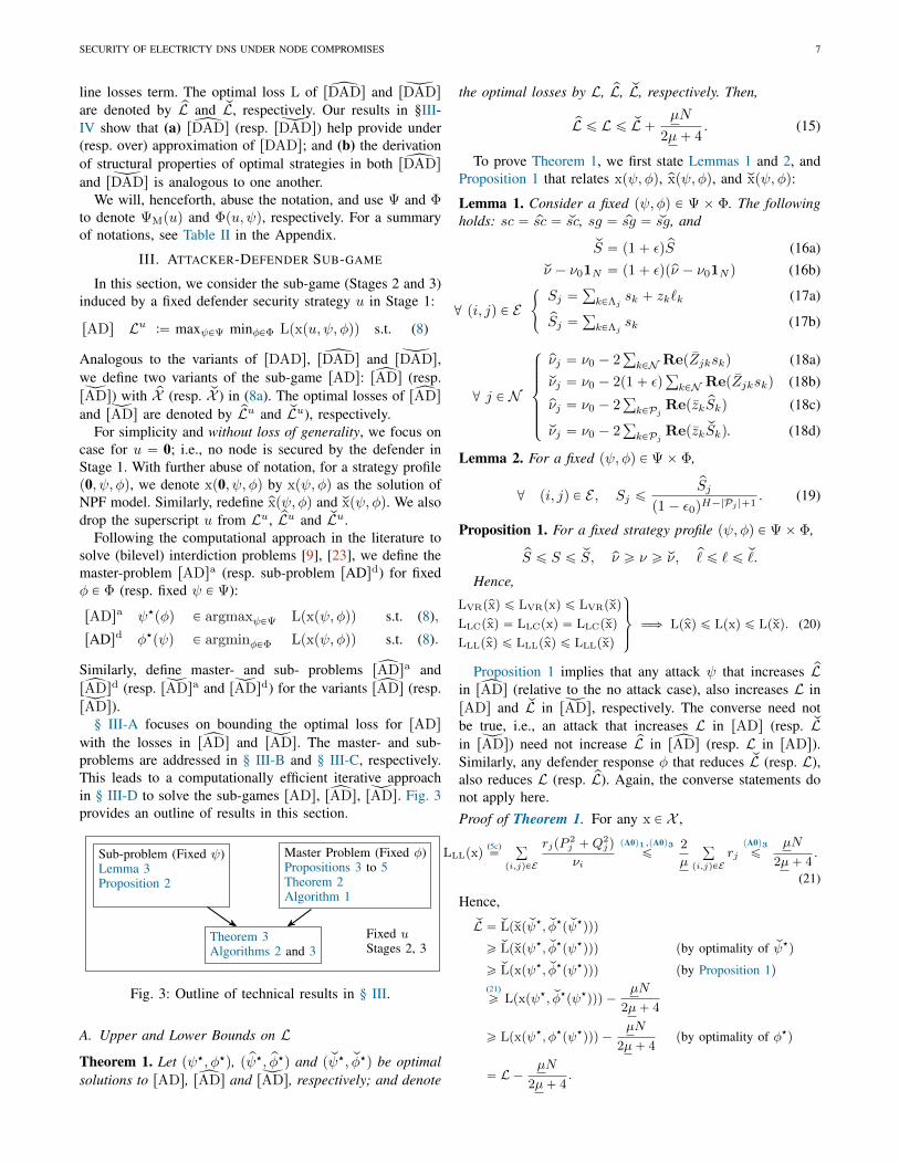
with the losses in ryADs and rADs. The master- and sub-problems are addressed in § III-B and § III-C, respectively.This leads to a computationally efficient iterative approachin § III-D to solve the sub-games rADs, ryADs, rADs. Fig. 3provides an outline of results in this section.

Sub-problem (Fixed ψ)Lemma 3Proposition 2

Master Problem (Fixed φ)Propositions 3 to 5Theorem 2Algorithm 1

Theorem 3Algorithms 2 and 3

Fixed uStages 2, 3

Fig. 3: Outline of technical results in § III.

A. Upper and Lower Bounds on LTheorem 1. Let pψ‹, φ‹q, p pψ‹, pφ‹q and p qψ‹, qφ‹q be optimalsolutions to rADs, ryADs and rADs, respectively; and denote

the optimal losses by L, pL, qL, respectively. Then,

pL ď L ď qL`µN

2µ` 4. (15)

To prove Theorem 1, we first state Lemmas 1 and 2, andProposition 1 that relates xpψ, φq, pxpψ, φq, and qxpψ, φq:

Lemma 1. Consider a fixed pψ, φq P Ψ ˆ Φ. The followingholds: sc “ psc “ qsc, sg “ psg “ qsg, and

qS “ p1` εqpS (16a)qν ´ ν01N “ p1` εqppν ´ ν01N q (16b)

@ pi, jq P E#

Sj “ř

kPΛjsk ` zk`k (17a)

pSj “ř

kPΛjsk (17b)

@ j P N

$

’

’

’

’

&

’

’

’

’

%

pνj “ ν0 ´ 2ř

kPN RepZjkskq (18a)qνj “ ν0 ´ 2p1` εq

ř

kPN RepZjkskq (18b)

pνj “ ν0 ´ 2ř

kPPj Repzk pSkq (18c)

qνj “ ν0 ´ 2ř

kPPj Repzk qSkq. (18d)

Lemma 2. For a fixed pψ, φq P Ψˆ Φ,

@ pi, jq P E , Sj ďpSj

p1´ ε0qH´|Pj |`1. (19)

Proposition 1. For a fixed strategy profile pψ, φq P Ψˆ Φ,

pS ď S ď qS, pν ě ν ě qν, p` ď ` ď q`.

Hence,

LVRppxq ď LVRpxq ď LVRpqxq

LLCppxq “ LLCpxq “ LLCpqxq

LLLppxq ď LLLppxq ď LLLpqxq

,

/

.

/

-

ùñ Lppxq ď Lpxq ď Lpqxq. (20)

Proposition 1 implies that any attack ψ that increases pLin ryADs (relative to the no attack case), also increases L inrADs and qL in rADs, respectively. The converse need notbe true, i.e., an attack that increases L in rADs (resp. qLin rADs) need not increase pL in ryADs (resp. L in rADs).Similarly, any defender response φ that reduces qL (resp. L),also reduces L (resp. pL). Again, the converse statements donot apply here.Proof of Theorem 1. For any x P X ,

LLLpxq(5c)“

ř

pi,jqPE

rjpP2j `Q

2j q

νi

pA0q1,pA0q3ď

2

µ

ř

pi,jqPErjpA0q3ď

µN

2µ` 4.

(21)

Hence,qL “ qLpqxp qψ‹, qφ‹p qψ‹qqq

ě qLpqxpψ‹, qφ‹pψ‹qqq pby optimality of qψ‹q

ě qLpxpψ‹, qφ‹pψ‹qqq pby Proposition 1q(21)ě Lpxpψ‹, qφ‹pψ‹qqq ´

µN

2µ` 4

ě Lpxpψ‹, φ‹pψ‹qqq ´µN

2µ` 4pby optimality of φ‹q

“ L´µN

2µ` 4.

8 IEEE TRANSACTIONS ON CONTROL OF NETWORK SYSTEMS

Similarly, one can show L ě pL.

Theorem 1 implies that the value of the sub-game rADswith NPF can be lower (resp. upper) bounded by the valueof ryADs (resp. rADs). Our subsequent results show that bothryADs and rADs admit computationally efficient solutions.

B. Optimal defender response to fixed attacker strategy ψ

We consider the sub-problem rADsd of computing optimaldefender response φ‹pψq for a fixed attack ψ.

The following Lemma shows that rADsd is a Second-OrderCone Program (SOCP), and hence, can be solved efficiently.

Lemma 3. Let XCPF :“ convpX q denote the set of states xsatisfying (2)-(4), (5a), (5b), and the relaxation of (5c):

For a fixed ψ P Ψ, the problem of minimizing Lpxpψ, φqqsubject to x P XCPF, (8b), (8c) is a SOCP. Its optimal solutionis also optimal for rADsd.

For fixed ψ (attack) and fixed load control parameter γ(e.g. when changing γ is not allowed), Proposition 2 belowprovides a range of optimal defender set-points pspd‹ and qspd‹

for LPF and ε-LPF models, respectively. Note that, if γ isfixed, LLCppxq is also fixed. Then, the defender set-pointscan be chosen by using LVRppxq as a loss function, insteadof pLppxq. Similar argument holds for qLpqxq.

Proposition 2. If we fix γ P Γ in ryADsd, then @i P N ,

δi “ 0 ùñ

∣∣∣ pspd‹i∣∣∣ “ spi, = pspd‹i P rarccotK, arccotKs.

Furthermore, if the DN has identical rx ” K ratio, then

δi “ 0 ùñ

∣∣∣ pspd‹i∣∣∣ “ spi, = pspd‹i “ arccotK. (22)

Similar results hold for rADsd.

C. Optimal attack under fixed defender response φ

Now, we focus on the master problem rADsa, i.e., theproblem of computing optimal attack for a fixed defenderresponse φ. The following Theorem characterizes the optimalattacker set-point, denoted by spa‹i “ Repspa‹i q`jImpsp

a‹i q,

when δi “ 1 (i.e. DER at node i is targeted by the attacker).

Theorem 2. Consider rADsa for a fixed δ P DM (i.e., theDERs compromised by the attacker are specified by δ andthe only decision variables in rADsa are spa). Then

@ i P N s.t. δi “ 1, spa‹i “ 0´ jspi. (23)

Same holds for both ryADsa and rADsa.

Proof. If δi “ 1, then pgi “xpgi “ Repspiq “ Repspa‹i q.We first prove the simpler case for ryADsa. From (6), one

can check that as functions of xpgi, pP is strictly decreasing,pQ is constant, and pν is strictly increasing. Hence, pLpψ, φf qis strictly increasing in xpgi (because LVR is non-decreasingas pν is decreasing; LLC is constant). Hence, to minimizethe loss L, the attacker chooses Rep pspa‹i q “ 0. Similarly,Imp pspa‹i q “ ´jspi. Similarly, we can show that in rADsa,qspa‹ “ 0´ jsp.

For the proof of spa‹ “ 0 ´ jsp, please refer to thesupplementary material at the end of the document.

(0,−spi) =: spa∗i (when δ∗i = 1)

Re(spi)

spi

Im(spi)

Optimal attacker set-point

for [AD], [AD], and [AD]

Range of Defender

Set-points spd∗ (resp. spd∗)for [AD] (resp. [AD])

when (δ∗i = 0)

Kspi√

K2+1, spi√

K2+1

Kspi√

K2+1, spi√

K2+1

quadrant I

quadrant IV

Fig. 4: Optimal attacker set-points (Theorem 2) and rangefor optimal defender set-points (Proposition 2).

Fig. 4 shows the optimal attacker set-point spa‹i for δ‹i “ 1,and the defender set-points for the DERs for δ‹j “ 0.

Thanks to Theorem 2, sc and sg are determined by δ and φ(since optimal spa‹ is given by (23)). Thus, for given pδ, φq,loss function can be denoted as Lpxp

“

0´ jsp, δ‰

, φqq; andrADs can be restated as follows:

L “ maxδPDMminφPΦ Lpxpδ, φqq s.t. (8), (23).

Same holds for ryADs (resp. rADs) and ryADsa (resp. rADsa).Note that the attacker actions on DERs may not be limited toan incorrect set-point attack. For example, the attacker cansimply choose to disconnect the DER nodes by choosingspa “ 0 ` 0j. However, Theorem 2 shows that the attackerwill induce more loss to the defender by causing the DERsto withdraw maximum reactive power rather than simplydisconnecting them.

Let ∆jppνiq (resp. ∆δppνiq) be the change in voltage atnode i caused due to compromise of DER at node j (resp.compromise of DERs due to attack vector δ.) Similarly,define ∆jpqνiq and ∆δpqνiq. We now state a useful result:

Lemma 4. If φ is fixed, then

@ i, j P N#

∆jppνiq “ 2RepZijpspdj ` jspjqq (24a)

∆jpqνiq “ 2p1` εqRepZijpspdj ` jspjqq (24b)

@ δ Ď DM

#

∆δppνiq “ř

j:δj“1 ∆jppνiq (25a)

∆δpqνiq “ř

j:δj“1 ∆jpqνiq. (25b)

For a fixed φ P Φ, let pDiMpφq be the set of optimal attack

vectors that maximize voltage bounds violation under LPF ata pivot node, say i. Formally,

pDiMpφq :“ argmax

δPDM

Wipνi ´ pνiq s.t. pxpδ, φq P pX , (8b), (8c) (26)

Also, letpD‹Mpφq :“

ď

iPN

pDiMpφq (27)

SECURITY OF ELECTRICTY DNS UNDER NODE COMPROMISES 9

denote the set of candidate optimal attack vectors, and pδi PpDi

Mpφq denote any vector in pDiM. Similarly, define qDi

Mpφq,qD‹Mpφq, and qδi.

Using Lemma 4, Algorithm 1 computes optimal pδ‹ tomaximize LVR for a fixed defender action φ P Φ [20]. Ineach iteration, the Algorithm selects one node as a pivot node.For a pivot node, say i, a set of target nodes pδi is determinedby selecting M nodes with largest ∆jppνiq (see Algorithm 5in Appendix). Applying Lemma 4, the final nodal voltage atthe current pivot node i is given by pνi´∆

pδippνiq. The attackstrategy that maximizes LVR is the set pδk corresponding to apivot node k that admits maximum voltage bound violationwhen DERs specified by pδk are compromised. Algorithm 1repeatedly calls procedure Algorithm 5, considering eachnode as the pivot node, and hence, requires Opn2 log nq time.

Algorithm 1 Optimal Attack for Fixed Defender Response

1: pδ‹pφq ÐOPTIMALATTACKFORFIXEDRESPONSE(φ)2: procedure OPTIMALATTACKFORFIXEDRESPONSE(φ)3: Compute state vector for no attack pxp0, φq P pX4: for i P N do5: pδi Ð GETPIVOTNODEOPTIMALATTACKpi, spd

q, andcalculate ∆

pδippνiq using Lemma. 46: Calculate new voltage value pν1i Ð pνi ´∆

pδippνiq7: end for8: k Ð argmaxiPN Wipνi ´ pν1iq

9: return pδ Ð pδk (Pick pδk which maximally violates (1))10: end procedure11: procedure GETPIVOTNODEOPTIMALATTACK(i, spd)12: pJ,Ngi ,m

1q Ð OPTIMALATTACKHELPER(i, spd)

13: Randomly choose M´m1 nodes from Ngi to form N 1

14: return pδi P DM such that pδik “ 1 ðñ k P J YN 1

15: end procedure

The following proposition argues that Algorithm 1 com-putes the optimal attack vectors for ryADsa and rADsa.

Proposition 3. For a fixed φ P Φ, if pδ is the optimal attackvector computed by Algorithm 1, then pδ is also an optimalattack vector of ryADsa. Same holds for rADsa.

We now show that the effect of DER compromise at eithernode j or k on the node i depends upon the locations of nodesj and k relative to node i. The following Proposition statesthat if node j is upstream to node k relative to the pivot nodei (j ăi k), then the DER compromise at node k impacts onpνi more than the DER compromise on node j; and if j “i k,then the effect of DER compromise at j, k on pνi is identical.

Proposition 4. [20] Consider ryADsa. Let nodes i, j, k P Nwhere i is the pivot node, spd

j “ spdk, and spj “ spk. If

j ăi k (resp. j “i k), then ∆jppνiq ă ∆kppνiq (resp. ∆jppνiq “

∆kppνiq). Same holds true for rADsa.

We, now, state a result that connects the optimal attackstrategies for ryADsa and rADsa.

Proposition 5. For a fixed φ P Φ, the following holds:1) The sets of candidate optimal attack vectors that max-

imizes voltage bound violations under LPF and ε-LPF are

identical, i.e.,pD‹Mpφq ” qD‹Mpφq. (28)

2) Furthermore, assume that νi “ νj “: ν and Wi “

Wj “: W @ i, j P N . Also, let the sets of optimal attackstrategies for ryADsa and rADsa be denoted by pΨ‹Mpφq andqΨ‹Mpφq, respectively. Let pψ‹ P pΨ‹Mpφq and qψ‹ P qΨ‹Mpφq beany two attack strategies. Now, if

LVRppxp pψ‹, φqq ą 0 and LVRpqxp qψ

‹, φqq ą 0, (29)

then the sets of optimal attack strategies for ryADsa andrADsa are identical, i.e.,

pΨ‹Mpφq ”qΨ‹Mpφq. (30)

As we will see in § III-D, Proposition 5 forms the basisof our overall computational approach.

D. A greedy approach for solving ryADs, rADs and rADs

We now utilize results for sub- and master-problems tosolve rADs. Consider the following assumption:(A1) DN has identical rx ” K ratio, i.e., @j P N ,Kj “ K.In this subsection, we present an algorithm to solve ryADs andrADs under (A0) and (A1), and then propose its extension, agreedy iterative approach, for solving rADs under the generalcase.

Under (A0) and (A1), the optimal defender set-pointspspd‹ and qspd‹ are as specified by Proposition 2, and hencefixed. For fixed optimal pspd‹ (resp. qspd‹), we can solve theproblem ryADs (resp. rADs) by using Benders Cut method[23]. However, we present a computationally faster algorithm,Algorithm 2 that computes attacker’s candidate optimal at-tack vectors pD‹M (resp. qD‹M) using Lemma 4.

Lemma 5. Under (A0), (A1), for any two fixed pγ1, pγ2 P Γ,pD‹Mp

“

pspd‹, pγ1‰

q “ pD‹Mp“

pspd‹, pγ2‰

q. Same holds true for qD‹M.

Given pspdP S , it can be checked that Algorithm 2, in fact,

computes pDiMp psp

dq, and pD‹Mp pspd

q “Ť

iPNpDi

Mp pspdq is the

set of candidate optimal attack vectors. The cardinality of theset pDi

M (Line 4) in the worst-case can be as high as Opene q.Therefore, computing pD‹M can take Opn exp pne qq time in theworst-case.

Algorithm 2 computes the set of attacks pD‹Mp pspd‹q, and

iterates over each pδ P pD‹Mp pspd‹q. In each iteration, since

spd “ pspd‹ is fixed, the sub-problem ryADsd reduces to anLP over the variable γ. Let pγ‹ppδq be the solution to the LP.Then, pφ‹ppδq “

“

pspd‹, pγ‹ppδq‰

is the optimal solution to ryADsd.Choosing pδ‹ “ argmax

pδP pD‹MLppxppδ, pφ‹ppδqqq, Algorithm 2

computes the solution to be ppδ‹, pφ‹ppδ‹qq to the problemryADs. Similarly, we can use Algorithm 2 to solve rADs.

Theorem 3. Under (A0), (A1), let ppδ, pφq be a solutioncomputed by Algorithm 2. Then ppδ, pφq is also an optimalsolution to ryADs. Similar result holds for rADs.

Proof. Under (A1), spd “ pspd‹ is fixed (Proposition 2).Then, for any γ P Γ, by Lemma 5 and Proposition 3, theoptimal attack pδ‹ belongs to the set pD‹Mp pspd‹

q. Algorithm 2

10 IEEE TRANSACTIONS ON CONTROL OF NETWORK SYSTEMS

Algorithm 2 Solution to ryADs for DNs with identical rx1: ppδ‹, pφ‹, pLq Ð GREEDY-ONE-SHOT()2: procedure GREEDY-ONE-SHOT()3: pL “ 0, pδ‹ “ 0, pγ‹ “ 1, pspd‹ as in Proposition 24: Let pDi

M “ GETPIVOTNODEOPTIMALATTACKSETpi, pspd‹q

5: pD‹M “Ť

iPNpDiM

6: For each pδ P pD‹M, compute pγ‹ppδq by solving ryADsd as anLP in γ. Let pφ‹ppδq “

pspd‹, pγ‹pδqqq

7: Let pδ‹ :“ argmaxpδP pD‹M

pLppxppδ,pγ‹ppδq, pspd‹qq

8: return pδ‹, pφ‹ “ pφ‹ppδ‹q, pL “ pLppxppδ‹, pφ‹qq9: end procedure

10: procedure GETPIVOTNODEOPTIMALATTACKSET(i, spd)11: pJ,Ngi ,m

1q Ð OPTIMALATTACKHELPER(i, spd)

12: return DiM Ð tpδ P DM|pδk “ 1 iff k P J Y

N 1, where N 1Ď Ngi and |N 1| “M ´m1u

13: end procedure

iterates over the attack vectors δ P pD‹M, computes pγ‹pδq bysolving an LP, and calculates the loss pLppxpδ, pφ‹pδqqq. Finally,it returns the solution corresponding to the maximum loss.Similar logic applies for optimal solution of rADs.

We, now, describe an iterative greedy approach to computethe solution to rADs that uses the optimal attacker strategyfor fixed defender response (refer Algorithm 1).

Algorithm 3 initializes φc to the optimal defender responseunder no attack. In the first step of the iterative approach,the attacker assumes some defender response φc to be fixed,and computes the optimal attack strategy δcpφcq using thegreedy Algorithm 1. Then in the second step, the defendercomputes a new defense strategy φc optimal for fixed δcby solving the SOCP, and updates the defender response. IfLpxpδc, φcqq ą Lpxpδ‹, φ‹qq, then the current best solutionpδ‹, φ‹q is updated to pδc, φcq. Then in the next iteration, theattacker uses this new defender response to update his attackstrategy, and so on and so forth. If this δc has already beendiscovered in some previous iteration, the algorithm termi-nates successfully, with δ‹, φ‹ as the required optimal attackplan, and the corresponding optimal defense. The algorithmterminates unsuccessfully if the number of iterations exceedsa maximum limit.

Note that in each iteration, the size of Υ increases by 1,hence, the algorithm is bound to terminate after exhaustingall possible attack vectors.

Proposition 5 and Theorem 3 can be applied for any u PUB , since if the DN has identical rx ratio, spd are also fixed.

Our overall computational approach to solving the problemrADs, thus far, can be summarized as in Fig. 5. Given aninstance of the problem rADs, we first solve the problemsryADs and rADs. For this, we employ an iterative procedurethat iterates between the master- and sub- problems. Fora fixed attacker action we determine the optimal defenderresponse φ for the rADsd using the convex relaxation of(5c). Then, for the fixed defender response φ, we computethe optimal attacker strategies pψ‹ and qψ‹ by solving ryADsa

and rADsa, respectively. Proposition 5 provides us an useful

Algorithm 3 Iterative Algorithm for Greedy Approach1: pδ‹, φ‹,Lq Ð GREEDY-ITERATIVE()2: procedure GREEDY-ITERATIVE3: Let δ‹ Ð 0,L‹ Ð 0, δc Ð 0, iter Ð 0,Υ ÐH, φc, φ

‹,Υ4: For δ “ δc, compute φ‹ by solving SOCP rADsd

(Lemma 3)5: φc Ð φ‹,L‹ Ð Lprxpδ, φ‹qq6: for iter Ð 0, 1, . . . ,maxIter do7: δc Ð OPTIMALATTACKFORFIXEDRESPONSE(φc)8: If δc previously found, successfully terminate9: if δc P Υ then return δ‹, φ‹

10: else Υ “ Υ Y tδcu Store the current best attackvector

11: Compute φc by solving SOCP rADsd Lemma 312: if Lprxpδc, φcqq ą L‹ then13: δ‹ Ð δc, φ

‹Ð φc,L‹ Ð Lprxpδ, φ‹qq

14: end if15: end for Maximum Iteration Limit reached16: Return δ‹, φ‹,L‹ Return the last best solution17: end procedure Algo terminates unsuccessfully

Lower bound ryADspL “ maxψ minφ pLppxpψ, φqq

s.t. px P pX

Fixed defender actionpψ‹ “ maxψ pLppxpψ, φf qq

s.t. px P pX

Upper bound rADsqL “ maxψ minφ qLpqxpψ, φqq

s.t. qx P qX

Fixed defender actionqψ‹ “ maxψ qLpqxpψ, φf qq

s.t. qx P qX

rADsL “ maxψ minφ Lpxpψ, φqqs.t. x P X

Fixed attacker actionφ‹ “ minφ Lpxpψf , φqqs.t. x P X

Proposition 5pΨ‹Mpφq ”

qΨ‹Mpφq

φf

φf

convergence ψf

Fig. 5: Overall computational approach.

result that ψ‹pφq :“ pψ‹ “ qψ‹. This optimal attacker strategyψ‹pφq is then fed back to the master- problem rADsa. Thisprocedure is repeated until we reach a convergence or weexceed the maximum iteration limit.

IV. SECURING DERS TO WORST-CASE ATTACKS

In this section, we consider the defender problem of opti-mal security investment in Stage 1. For simplicity, we restrictour attention to DNs that satisfy the following assumption:(A2) Symmetric Network. For every i P N , for any twonodes j, k P N c

i , Λj and Λk are symmetrically identical aboutnode i. That is, zj “ zk,

∣∣N cj

∣∣ “ |N ck |, scnom

j “ scnomk ,

νj “ νk, Wj “ Wk, and Cj “ Ck. However, all the DERsare homogeneous, i.e., @ j, k P N , spj “ spk.

Let B be a fixed security budget. Let u, ru P UB , u ‰ ru,be two security strategies. Strategy u is more secure thanstrategy ru (denoted by u ď ru) under NPF (resp. LPF), ifLu ď Lru (resp. pLu ď pLru). Finally, we ask what is the bestsecurity strategy u‹, such that for u “ u‹, Lu is minimized.Fig. 6 shows two possible security strategies u1 (Fig. 6a) andu2 (Fig. 6b), and gives a generic security strategy (Fig. 6c).If we compare u1 and u2, while transitioning from u1 tostrategy u2, 3 secure nodes in Λ2 subtree go up a level each,while 3 secure nodes in Λ3 subtree go down a level each.Then, between u1 and u2, which strategy is more secure?In this section, we provide insights about optimal security

SECURITY OF ELECTRICTY DNS UNDER NODE COMPROMISES 11

strategies under (A2), which help show that u2 is more securethan u1.

0

1

3

4 5 6 7

8 9 10 11 12 13 14 15

2

4

(a) Security strategy u1.Nspu1q “ t3, 5, 6, 7, 10, 11u.

0

1

2 3

4 5 6 7

8 9 10 11 12 13 14 15

(b) Security strategy u2.Nspu2q “ t2, 4, 5, 6, 12, 14u.

b

ai′ i′′

d

c0Vulnerable nodes

Secure nodes

(c) A generic security strategy on a tree DN.

Fig. 6: Different defender security strategies.

Algorithm 4 computes an optimal security strategy rzDADsunder (A0)-(A2). It initially assigns all nodes to be vulnera-ble. Then, DER nodes are secured sequentially in a bottom-upmanner towards the root node. If the security budget is notadequate to secure a full level, the nodes in that level areuniformly secured and the remaining nodes are not secured.Under all the assumptions of Algorithm 4, it takes Opnq time.

Algorithm 4 Optimal security strategy1: pu‹ ÐOPTIMALSECURITYSTRATEGY()2: procedure OPTIMALSECURITYSTRATEGY()3: ns Ð 0, h Ð H , pu Ð 0 Initialize all nodes to

vulnerable nodes4: For each h P r1, 2, . . . , Hs, let αh Ð

řHj“h |Nj |

5: Let h1 Ð argmaxhPr1,...,Hs:αhěM h6: Let @ h P rh1, . . . , Hs,@ i P Nh, pui Ð 1.7: Let N 1

h1 Ď Nh1 be a set of uniformly chosen M ´ αh1`1

nodes on level h1.8: For each i P N 1

h1 , pui Ð 19: return pu

10: end procedure

In the following theorem, we show that the securitystrategy computed by Algorithm 4 is an optimal solution tothe Stage 1 of the rzDADs and r~DADs problem.

Theorem 4. Assume (A0), (A1), (A2). Let pu‹ be the securitystrategy computed by Algorithm 4. Furthermore, with u “ pu‹,let p pψ‹, pφ‹q be the solution computed by Algorithm 2. Then,ppu‹, pψ‹, pφ‹q is an optimal solution to rzDADs. Similar resultholds for r~DADs.

Finally, we state the following result:

Proposition 6. 1) Under (A0), (A1), (A2), pD‹M can bepartitioned into at most |Nv| ď N equivalence classes ofattack vectors, one for each vulnerable node considered aspivot node. Any two attack vectors in the same equivalence

class has identical impact on the corresponding pivot node.Additionally, any two equivalence classes can be consideredhomomorphic transformations of each other.

2) Under (A0), (A1), if @ i, j, k P N such that spj ą 0 and

spk ą 0, ∆jppνiq ‰ ∆kppνiq, then∣∣∣ pD‹M

∣∣∣ “ |Nv|, i.e., if forany pivot node, no two DERs have identical impact on thepivot node due to their individual DER compromises, theneach equivalence class is a singleton set, and hence, the setfor candidate optimal attack vectors is at most of size |Nv|.

By Theorem 4, we can compute the optimal securityinvestment pδ‹ in OpNq, and by Proposition 6, for fixedpδ‹, we can compute the optimal attacker strategy pψ‹ inOpNq. Finally, for fixed pδ‹ and pψ‹, we can compute theoptimal defender response pφ‹ in OppolypNqq. Hence, we cancompute the optimal solution for rzDADs, in OppolypNqq.Same holds for r~DADs.

Admittedly, our structural results on optimal security in-vestment in Stage 1 of the game are specific to assump-tion (A2). Future work involves extending these results toa general radial DN with heterogeneous DER nodes. A keyaspect in effort will be to understand how the defender’s netvalue of securing an individual DER node depends on itscapacity and location in the DN.

V. COMPUTATIONAL STUDY

We describe a set of computational experiments to evaluatethe performance of the iterative Greedy Approach (GA) insolving rADs; see Algorithm 3. We again assume u “ 0. Wecompare the optimal attack strategies and optimal defenderset-points obtained from GA with the corresponding solutionsobtained by conducting an exhaustive search (or Brute Force(BF)), and by implementing the Benders Cut (BC) algorithm.We refer the reader to [9], [23], for the BC algorithmadopted here. The abbreviations BC-LPF and BC-NPF denotethe solutions obtained by applying optimal attack strategiesfrom ryADs to LPF and NPF, respectively. Importantly, theexperiments illustrate the impact of attacker’s resource (M)and defender’s load control capability γ on the optimal valueof rADs. The code for this computational study can beobtained by contacting the authors.

Network Description: Our prototypical DN is a modifiedIEEE 37-node network; see Fig. 1. We consider two variantsof this network: homogeneous and heterogeneous. Homo-geneous Network (GI ) has 14 homogeneous DERs withrandomly assigned node locations, loads with equal nominaldemand, and lines with identical rx ratio. Each line hasimpedance of zj “ p0.33 ` 0.38jq Ω. The nominal demandat each node i is scnom

i “ 15 kW ` j4.5 kvar. The apparentpower capability of each DER node i is spi “ 11.55 kV A.The nominal voltage at node 0 is |V0| “ 4 kV . The cost ofload control is C “ 7 $ per kW . Heterogeneous Network(GH ) has same topology as GI , but has heterogeneous DERs(chosen at random from 3 different DER apparent powercapabilities), heterogeneous loads, and lines with differentrx ratios. The locations of DER nodes, the total nominalgeneration capacity, and the total nominal demand in GH is

12 IEEE TRANSACTIONS ON CONTROL OF NETWORK SYSTEMS

roughly similar to the corresponding values for GI .DER output vs M. Fig. 7 compares the DER output (sg) ofuncompromised DERs that form part of defender response inGI and GH for different M. When M “ 0 (no attack), thereare no voltage violations, and the defender minimizes LLL,which results in pg ą qg. For M ą 0, the voltage boundsmay be violated. To limit LVR, the defender responds byincreasing qg; and the output of uncompromised DERs liein a neighborhood of θ “ arccot rx. For the case of GH(Fig. 7b), the set-points of the uncompromised DERs aremore spread out to achieve voltage regulation over differentrx ratios (Proposition 2). In Fig. 7b the three semi-circlescorrespond to the uncompromised DERs with different ap-parent power capabilities. These observations on the defenderresponse validate Proposition 2.

pg in p.u.

0 0.01 0.02 0.03

qg i

n p

.u.

0

0.005

0.01

0.015

0.02

0.025

0.03

θ = arccotr

x

PV output range

M = 0

M = 2

M = 6

M = 7

(a) Homogeneous network.

pg in p.u.

0 0.01 0.02 0.03

qg i

n p

.u.

0

0.005

0.01

0.015

0.02

0.025

0.03

θ = arccotr

x

PV output ranges

M = 0

M = 2

M = 6

M = 7

(b) Heterogeneous network.

Fig. 7: Reactive power vs Real power output of DERs.

GA vs. BC-NPF, BC-LPF and BF. Fig. 8 compares resultsobtained from BC-NPF, GA, and BF on GI . We considertwo cases with the maximum controllable load percentageγ “ 50 % and γ “ 70 %. For each case, we vary M from 0to |Nv| “ 14; and also vary WC ratios to capture the effectof different weights on the terms LVR and LLC.

In our study, we chose Ci “ 7 centskWh, convertedappropriately to the per unit system. 6 The ratio WC “ 2roughly corresponds to the maximum WC ratio for which thedefender does not exercise load control, because the cost ofdoing load control is too high, i.e., at optimum defender re-sponse γ‹ “ 1N . In contrast, WC “ 18 roughly correspondsto the minimum WC ratio for which the defender exercisesmaximum load control (i.e. γ‹ “ γ). We also consider anintermediate ratio, WC “ 10.L versus M. Both LVR and LLC are zero when there is noattack. As M increases, one or both LVR and LLC start in-creasing. This indicates that as more DERs are compromised,the defender incurs LVR, and in addition, he imposes loadcontrol to better regulate the DN. Indeed, after the false set-points (Theorem 2) are used to compromise DERs, the netload in the DN increases. Without load control, the voltages

6From a practical viewpoint, the weights Ci can be obtained from theoperator’s rate compensation scheme for load control. For example, NorthStar Electric [24] provides a compensation of 9.1 cents to their customersfor 1 kWh of load curtailment. One can argue that the net cost of sheddingunit load should be adjusted to reflect the fact that the defender suppliesadditional power during the attack to meet the consumers’ demand.

0 5 10

M

0

500

1000

LVR(in$)

W

C= 2

W

C= 10

W

C= 18

BF

GA

BC NPF

BC LPF

(a) LVR vs M, γ “ 0.5.

0 5 10

M

0

500

1000

1500

2000

2500

LVR(in$)

W

C= 2

W

C= 10

W

C= 18BF

GA

BC NPF

BC LPF

(b) LVR vs M, γ “ 0.7.

0 5 10

M

0

500

1000

1500

LLC(in$)

W

C= 2

W

C= 10

W

C= 18

BF

GA

BC NPF

BC LPF

(c) LLC vs M, γ “ 0.5.

0 5 10

M

0

200

400

600

800

1000

LLC(in$)

W

C= 2

W

C= 10

W

C= 18

BF

GA

BC NPF

BC LPF

(d) LLC vs M, γ “ 0.7.

Fig. 8: LVR and LLC vs M for GI . The results of GH aremore or less similar to those of GI .

at some nodes drop below the lower bounds, increasing LVR.Hence, the defender exercises load control, and changes theset-points of uncompromised DERs to limit the total loss.

Perhaps a more interesting observation is that as M in-creases, LLC first increases rapidly but then flattens out(Figures 8c and 8d). This can be explained as follows:depending on the WC ratio, there is a subset of downstreamloads that are beneficial in terms of the value that thedefender can obtain by controlling them. That is, if theloads belonging to this subset are controlled, the decreasein LVR outweighs the increase in LLC, hence, the defenderimposes load control on these downstream loads to reducethe the total loss. In contrast, controlling the loads outsidethis subset, increases LLC more than the decrease in LVR.Hence, the defender satisfies the demand at these loadsfully. The LLC increases until load control capability in thesubset of beneficial downstream loads to the defender is fullyexhausted. The size of this subset depends on the WC ratio.The higher the ratio, the larger the size of the subset of theloads beneficial to the defender. Hence, the value of M, atwhich the LLC cost curve flattens out, increases as the WC

ratio increases.The cost curve for LVR also shows interesting behavior as

the number of compromised DER nodes increases (Figures 8aand 8b). The marginal increase in LVR for every additionalDER compromised reduces as M increases. This observationcan be explained by the fact that the attacker prefers tocompromise downstream nodes over upstream ones (Propo-

SECURITY OF ELECTRICTY DNS UNDER NODE COMPROMISES 13

sition 4). Initially, the attacker is able to rapidly increase Lby compromising more beneficial downstream nodes. How-ever, as the downstream nodes are eventually exhausted, theattacker has to target the relatively less beneficial upstreamnodes. Hence, the reduction in marginal increase of LVR.

In LVR plots, for small M, WC “ 2 curves are lower thanthe WC “ 10 curves which in turn are lower than the WC “

18 curves. But, for larger M, this order reverses. The M wherethese lines cross each other decreases, as the γ increases (seeFigures 8a and 8b). The reason is for some intermediate valueof M, the defender exhausts the load control completely, andthen the L increases at rates in the same order of increasingWC values.

Our computational study also validates that the GA is moreefficient than BC method because GA calculates the exactimpact the DER compromises will have on a pivot node. Incontrast, BC overestimates the impact of DER compromisesthat are not the ancestors to the pivot nodes. Therefore, thefeasible region probed by BC at every iteration is larger thanthe feasible region probed in the corresponding iteration ofGA. Hence, although GA converges to a solution in 2-3iterations, BC in most cases does not converge to the optimalsolution even in 200 iterations.

VI. CONCLUDING REMARKS

We focused on the security assessment of radial DNs for anadversary model in which multiple DERs (in this case, DERnodes) are compromised. The adversary can be a threat agent,who can compromise the operation of DERs, or a maliciousinsider in the control center. We considered a composite lossfunction that primarily accounts for the attacker’s impact onvoltage regulation and induced load control. The securityassessment problem is formulated as a three-stage Defender-Attacker-Defender (rDADs) sequential game. Our main tech-nical contributions include: (i) Approximating the rDADsgame that has nonlinear power flow model and mixed-integerdecision variables with tractable formulations based on linearpower flow; and (ii) characterization of structural propertiesof security investments in Stage 1 and the optimal attack inStage 2 (i.e., the choice of DER node locations and the choiceof false set-points).

Future work includes: (a) Extending Theorems 1 and 2to cases where reverse power flows are permissible (e.g.,when the DN is not under heavy loading conditions and theattacker can cause DER generation to exceed the demand);(b) Designing greedy algorithm to solve [AD] and provingoptimality guarantees of Theorems 3 and 4 for DNs withheterogeneous rx ratio, and heterogeneous DERs or loads.

Finally, note that we do not consider cascading failuresin our paper. However, our analysis can be extended to aform of cascading failures within DNs reported by Kunduand Hiskens [25]. They study synchronous tripping of theloads (specifically, plug-in electric vehicles chargers) leadingto over-voltages in the DN. Our result on optimal DER attackcan be used to create voltage violations at some nodes. Ifthese violations are too high, certain loads may start to trip.After sufficiently large number of loads trip, the attacker

can further manipulate the DER setpoints to their maximumpower generation capacity. In the absence of new loads, thismay lead to overvoltages, as described in [25].

REFERENCES

[1] I. A. Hiskens, “What’s smart about the smart grid?” in DesignAutomation Conference (DAC), 2010 47th ACM/IEEE, June 2010, pp.937–939.

[2] H. Fawzi, P. Tabuada, and S. Diggavi, “Secure estimation and controlfor cyber-physical systems under adversarial attacks,” IEEE Transac-tions on Automatic Control, vol. 59, no. 6, pp. 1454–1467, June 2014.

[3] Y. Mo, T. H. J. Kim, K. Brancik, D. Dickinson, H. Lee, A. Perrig, andB. Sinopoli, “Cyber-physical security of a smart grid infrastructure,”vol. 100, no. 1, Jan 2012, pp. 195–209.

[4] F. Pasqualetti, F. Drfler, and F. Bullo, “Attack detection and identi-fication in cyber-physical systems,” IEEE Transactions on AutomaticControl, vol. 58, no. 11, pp. 2715–2729, Nov 2013.

[5] K. C. Sou, H. Sandberg, and K. Johansson, “Computing critical k-tuples in power networks,” Power Systems, IEEE Transactions on,vol. 27, no. 3, pp. 1511–1520, Aug 2012.

[6] A. Teixeira, K. C. Sou, H. Sandberg, and K. H. Johansson, “Securecontrol systems: A quantitative risk management approach,” IEEEControl Systems, vol. 35, no. 1, pp. 24–45, Feb 2015.

[7] B. A. Robbins and A. D. Dominguez-Garcia, “Optimal reactive powerdispatch for voltage regulation in unbalanced distribution systems,”IEEE Transactions on Power Systems, vol. 31, no. 4, pp. 2903–2913,July 2016.

[8] K. Turitsyn, P. Sulc, S. Backhaus, and M. Chertkov, “Options forcontrol of reactive power by distributed photovoltaic generators,”Proceedings of the IEEE, vol. 99, no. 6, pp. 1063–1073, June 2011.

[9] J. Salmeron, K. Wood, and R. Baldick, “Analysis of electric gridsecurity under terrorist threat,” IEEE Transactions on Power Systems,vol. 19, no. 2, pp. 905–912, May 2004.

[10] ——, “Worst-case interdiction analysis of large-scale electric powergrids,” IEEE Transactions on Power Systems, vol. 24, no. 1, pp. 96–104, Feb 2009.

[11] Y. Yao, T. Edmunds, D. Papageorgiou, and R. Alvarez, “Trilevel op-timization in power network defense,” IEEE Transactions on Systems,Man, and Cybernetics, Part C (Applications and Reviews), vol. 37,no. 4, pp. 712–718, July 2007.

[12] A. A. Cardenas, S. Amin, Z.-S. Lin, Y.-L. Huang, C.-Y. Huang,and S. Sastry, “Attacks against process control systems: Riskassessment, detection, and response,” in Proceedings of the 6th ACMSymposium on Information, Computer and Communications Security,ser. ASIACCS ’11. New York, NY, USA: ACM, 2011, pp. 355–366.[Online]. Available: http://doi.acm.org/10.1145/1966913.1966959

[13] H. Zhang, P. Cheng, L. Shi, and J. Chen, “Optimal DoS attackscheduling in wireless networked control system,” IEEE Transactionson Control Systems Technology, vol. 24, no. 3, pp. 843–852, May 2016.

[14] M. Farivar, R. Neal, C. Clarke, and S. Low, “Optimal inverter VARcontrol in distribution systems with high PV penetration,” in 2012IEEE Power and Energy Society General Meeting, July 2012, pp. 1–7.

[15] A. Lee, “Electric sector failure scenarios and impactanalyses,” National Electric Sector Cybersecurity OrganizationResource (NESCOR), Electric Power Research Institute (EPRI),Palo Alto, California, Tech. Rep., June 2014. [Online].Available: http://www.smartgrid.epri.com/doc/NESCOR%20failure%20scenarios%2006-30-14a.pdf

[16] R. Lee, M. Assante, and T. Conway, “Analysis of the cyber attackon the Ukrainian power grid, electricity information sharing and anal-ysis center,” http://www.nerc.com/pa/CI/ESISAC/Documents/E-ISACSANS Ukraine DUC 18Mar2016.pdf, 2015.

[17] R. Campbell, “Cybersecurity issues for the bulk power system, con-gressional research service report,” https://www.fas.org/sgp/crs/misc/R43989.pdf, 2015.

[18] D. Shelar and S. Amin, “Security assessment of electricity distributionnetworks under DER node compromises,” 2015. [Online]. Available:https://arxiv.org/abs/1601.01342v3

[19] H. D. Chiang and M. E. Baran, “On the existence and uniquenessof load flow solution for radial distribution power networks,” IEEETransactions on Circuits and Systems, vol. 37, no. 3, pp. 410–416,Mar 1990.

14 IEEE TRANSACTIONS ON CONTROL OF NETWORK SYSTEMS

Parameters Valuesr ` jx p0.33` 0.38jq Ωpcnomi 15 kWqcnomi 4.5 kvar

spi 11.55 kV A|V0| 4 kVC 7 $ per kW

TABLE I: Parameters of the Homogeneous Network

[20] D. Shelar and S. Amin, “Analyzing vulnerability of electricity dis-tribution networks to DER disruptions,” in 2015 American ControlConference (ACC), July 2015, pp. 2461–2468.

[21] M. Farivar and S. H. Low, “Branch flow model: Relaxations andconvexification - part i,” IEEE Transactions on Power Systems, vol. 28,no. 3, pp. 2554–2564, Aug 2013.

[22] S. Amin, G. A. Schwartz, and S. Shankar Sastry, “Security ofinterdependent and identical networked control systems,” Automatica,vol. 49, no. 1, pp. 186–192, Jan. 2013. [Online]. Available:http://dx.doi.org/10.1016/j.automatica.2012.09.007

[23] R. Wood, “Bilevel network interdiction models: Formulations and solu-tions,” in Wiley Encyclopedia of Operations Research and ManagementScience, 2011.

[24] “Compensation of load control.” [Online]. Available: http://www.northstarelectric.coop/?page id=180

[25] S. Kundu and I. Hiskens, “Overvoltages due to synchronous trippingof plug-in electric-vehicle chargers following voltage dips,” PowerDelivery, IEEE Transactions on, vol. 29, no. 3, pp. 1147–1156, June2014.

[26] L. Gan, N. Li, U. Topcu, and S. H. Low, “Exact convex relaxationof optimal power flow in radial networks,” IEEE Transactions onAutomatic Control, vol. 60, no. 1, pp. 72–87, Jan 2015.

APPENDIX

For a pivot node i P N , Algorithm 5 computes a sequenceof sets of nodes in decreasing order of ∆jppνiq values.This sequence is used to compute the optimal attacks thatmaximize voltage bounds violation at node i.

Algorithm 5 Helper procedure1: procedure OPTIMALATTACKHELPER(i, pspd)2: For each j P N compute ∆jppνiq using Lemma 43: Create a sequence of sets tN i

j uNj“1 such that

i) N “ŤNj“1 N

ij , @ 1 ď j, k,ď N, N i

j XN ik “ H

ii) if 1 ď l ď N, j, k P N il , then ∆jppνiq “ ∆kppνiq, and

iii) if 1 ď l ă m ď N, j P N il , k P N i

m, then ∆jppνiq ą∆kppνiq.

4: Let, for j P r1, . . . , N s,mij Ð

∣∣N ij

∣∣, M ij :“

řj´1k“1m

ik.

5: Let gi Ð argminjPr1,...,Ns,MijěM

j.

6: J ÐŤgi´1j“1 , Ngi , m

1“M ´M i

gi´1

7: return J , Ngi , m1

8: end procedure

j j “?´1 complex square root of -1

Network parametersN set of nodesE set of edgesG tree topology G “ pN , Eqrj resistance of line pi, jq P Exj reactance of line pi, jq P Ezj impedance zj “ rj ` jxj of line pi, jq P EH height of the treeNh set of nodes on level h P 1, 2, ¨ ¨ ¨ , Hhi level of node iN ci set of children nodes of node i

Λi subtree rooted at node i P NΛji subtree rooted at node i P N until level hj for j P ΛiPi path from the root node to node iZij Zij :“

ř

kPPiXPj zk common path impedances be-tween nodes i and j

Power flow notationsNPF Nodal quantities of node i P N LPF ε-LPFscnomi complex power demand at node i ´ ´

sci complex power consumed at node i psci qscisgi complex power generated at node i xsgi |sgispi complex power set-point of DER i pspi qspiVi complex voltage at node i pVi qViνi square of voltage magnitude at node i pνi qνiνi, νi soft lower and upper bounds on square

of voltage magnitude at node iNPF Edge quantities of edge pi, jq P E LPF ε-LPFSj complex power flowing on line pi, jq pSi qSi

Ij complex current flowing on line pi, jq pIi qIi

`j square of magnitude of current Ij p`i q`ix x “ pν, `, sc, sg, Sq - state vector px qx

Attacker modelδi δi “ 1 if DER i is compromised ´ ´

spai attacker set-point of DER i pspa

i qspai

ψ ψ :“ pspa, δq attacker strategy pψ qψ

Defender modelγi

max. allowed fraction of load control ´ ´

γi fraction of load control at load i pγi qγispdi defender set-point of DER i pspd

i qspdi

φ φ :“ pspd, γq defender strategy pφ qφ

TABLE II: Table of Notations.

Devendra Shelar is pursuing his Ph.D. at the Cen-ter for Computational Engineering (CCE), Mas-sachusetts Institute of Technology (MIT). He is in-terested in developing tools using large-scale opti-mization and game theory to improve the resiliencyof cyber-physical systems to failures. His currentfocus is on the secure and efficient operation ofpower systems with high penetration of distributedenergy resources. He received his Dual B.Tech.& M.Tech. in Computer Science and Engineeringfrom the Indian Institute of Technology Bombay

in 2012, M.S. in Transportation Engineering from MIT in 2016.

SECURITY OF ELECTRICTY DNS UNDER NODE COMPROMISES 15

Saurabh Amin is Robert N. Noyce Career De-velopment Assistant Professor in the Departmentof Civil and Environmental Engineering, Mas-sachusetts Institute of Technology (MIT). His re-search focuses on the design and implementationof high confidence network control algorithms forinfrastructure systems. He works on robust diag-nostics and control problems that involve usingnetworked systems to facilitate the monitoring andcontrol of large-scale critical infrastructures, in-cluding transportation, water, and energy distribu-

tion systems. He also studies the effect of security attacks and random faultson the survivability of networked systems, and designs incentive-compatiblecontrol mechanisms to reduce network risks. Dr. Amin received his Ph.D. inSystems Engineering from the University of California, Berkeley in 2011.He is a recipient of NSF CAREER award, and Google Faculty Researchaward.

16 IEEE TRANSACTIONS ON CONTROL OF NETWORK SYSTEMS

SUPPLEMENTARY MATERIAL

Proof of Lemma 1. Recursively apply the power flow mod-els (5), (6), and (12), from the root node to leaf nodes.

Proof of Lemma 2. We apply induction from leaf nodes tothe root node. Base case: For any leaf node k P NL,

zk`kpA0q4ď ε0Sk

(17a)“ ε0psk ` zk`kq

6 zk`k ďε0sk

1´ ε0

(17b)“

ε0 pSk1´ ε0

.

Now, for any j P N zNL,

zj`jpA0q4ď ε0Sj

(5a)“ ε0

“ř

k:pj,kqPE Sk ` sj ` zj`j‰

6 zj`j ďε0

1´ ε0

“ř

k:pj,kqPE Sk ` sj‰

.

Addingř

Sk ` sj on both the sides:

ř

k:pj,kqPE Sk ` sj ` zj`jlooooooooooooooomooooooooooooooon

Sj

ď1

1´ ε0

“ř

k:pj,kqPE Sk ` sj‰

.

Inductive step: By inductive hypothesis (IH) on N cj ,

Sj(IH)ď

1

p1´ ε0qH´|Pk|`2

“ř

k:pj,kqPEpSk ` sj

‰

“pSj

p1´ ε0qH´|Pj |`1p7 |Pj | “ |Pk|´ 1q.

Proof of Proposition 1. The inequalities pS ď S and pν ě νare proved in [26].

The rest of the proof of Proposition 1 utilizes two lemmas.From Lemma 2, for any pi, jq P E ,

Sj ďpSj

p1´ ε0qH´|Pj |`1ď

pSjp1´ ε0qH

“ p1` εqpSj(16a)“ qSj .

(31)For nodal voltages,

νj(5b)“ νi ´ 2RepzjSjq ` |z|2j `jě νi ´ 2RepzjSjq(31)ě νi ´ 2Repzj qSjq. (32)

Applying (32) recursively from the node j till root node:

νj ě ν0 ´ 2ř

kPPj Repzk qSkq(18d)“ qνj .

Thus, pSj ď Sj ď qSj and pνj ě νj ě qνj . Furthermore,

pSj ď Sj ď qSjpA0q2ùñ

∣∣∣pSj∣∣∣2

ď |Sj |2 ď∣∣∣qSj

∣∣∣2

ùñ

∣∣∣pSj∣∣∣2

pνjď

|Sj |2νj

ď

∣∣∣qS∣∣∣2

qνjùñ p` ď ` ď q`.

Finally, (20) immediately follows from (9), (10), and (15).

Proof of Lemma 3. Let rĄADsd denote the following prob-lem:

rĄADsd rφ‹pψq P argminφPΦ

Lpxpψ, φqq

s.t. pxpu, ψ, φq P XCPF, (8b), (8c).(33)

pA0q1 implies that a feasible solution exists for rADsd.Since, X Ă XCPF, a feasible solution rx P XCPF also exists forrĄADsd.

Let prφ, r`q denote the decision variables for rĄADsd. Notethat, for a fixed ψ, rx is affine in the variables prφ, r`q, and canbe very efficiently computed using (5a) and (5b).

Now, L is convex in rφ (because the LVR is a maximumover affine functions, LLC is affine in rφ, and LLL is affine inr`. Also, Φ is a convex compact set. Further, for a fixed φ, Lis strictly increasing in r` (because, LVR is non-decreasing inr` as rν is affine decreasing in r`; LLC does not change with r`;LLL is strictly increasing in `). From Theorem 1 [21], prφ‹, r`‹qcan be computed using a SOCP. To argue that r`‹ satisfy(5c), assume for contradiction that D pi, jq P E , s.t. r`‹j ą∣∣∣ rS‹j ∣∣∣2rν‹i . Then, construct pφ‹, r`1q such that @ j P N : j ‰

i, r`1j “r`‹j , and r`1i “

∣∣∣ rS‹j ∣∣∣2rν‹i . Since @ pj, kq P E , ∣∣∣ rSk∣∣∣2rνjis strictly decreasing in r`i, @ pj, kq P E : r`1k ě

∣∣∣ rS‹k∣∣∣2rν‹j ą∣∣∣ rS1k∣∣∣2rν1j . Hence, one can further minimize the loss function

by choosing a new feasible solution pφ‹, r`1q, thus violatingthe optimality of prφ‹, r`‹q.

Proof of Proposition 2. Let pdi, θiq denote pspdi in the polar

coordinates, i.e., di “∣∣∣ pspd

i

∣∣∣ , θi “ = pspdi .

For δi “ 0, pspi “ pspdi . Then from (18a), @ j P N ,

pνj “ pν1j ` 2dipRij cos θi `Xij sin θiq, (34)

where pν1j “ ν0 ´ 2ř

kPN ,k‰jRepZjkskq ´ 2RepZijscjq.Note that pν1j does not depend on pdi, θiq.

It is clear from (34) that pνj is greater if θi P r0, π2s thanif θi P r´π2, 0s. Furthermore, the impedances are positive.Hence, @ j, Bdipνj “ 2pRij cos θi ` Xij sin θiq ą 0. Hence,BdiLVR ą 0. But, from (4), di ď spi. Hence, d‹i “ spi.Further, Bθipνj “ 2dip´Rij sin θi `Xij cos θiq.

Bθipνj

$

’

&

’

%

ą 0 if θi P r0, arccotpRijXijqq

“ 0 if θi “ arccotpRijXijqq

ă 0 if θi P parccotpRijXijqq, π2s

Now, arccotK ď arccotpXijRijq ď arccotK. Hence,

@ j P N , Bθipνj

#

ă 0 if θi ą arccotK

ą 0 if θi ă arccotK(35)

Suppose, for contradiction, θ‹i R rarccotK, arccotKs. Hold-ing all else equal, for θi “ rθi, let pνprθiq and LVRprθiq be thepν and LVR. From (35), for any rθi P rarccotK, arccotKs,pνprθiq ą pνprθ‹i q. Since, LVR ą LLL ě 0, LVRprθiq ă LVRprθ

‹i q,

violating the optimality of rθ‹i . Furthermore, under identicalrx ratio, K “ K “ K, which implies θi “ arccotK.

Claim 1. Theorem 2 also holds for rADsa.

SECURITY OF ELECTRICTY DNS UNDER NODE COMPROMISES 17

Proof. Now, we prove the case for rADsa by contradiction.Suppose that there exists i P N s.t. Repspa‹i q ą 0. Then wecan construct another attacker strategy rψ‹ “ rrδ, rspa

s that canfurther maximize L, such that Repspa‹i q “ 0, holding all elseequal, i.e., rδ “ δ,@ j P N , Imp rspa

j q “ Impspa‹j q,@ j P N :j ‰ i, Rep rspa

j q “ Repspa‹j q.Let pspa, `q be the decision variables for rADsa, as for

fixed φ, the other decision variables P,Q, ν can then bewritten as affine functions of pspa, `q from (5). Let pspa‹, `‹q(resp. p rspa, r`q) be the solution to rADsa when ψ “ ψ‹ (resp.ψ “ rψ).

Let f P RN` such that, for any pi, jq P E , fjpspa, `q :“P 2j `Q

2j

νi. Let f‹ “ fpspa‹, `‹q, f 1 “ fp rspa, `‹q, and rf “

fp rspa, r`q.Since pspa‹, `‹q and p rspa, r`q are solutions to rADsa, they

satisfy (5c). Hence, f‹ “ `‹, and rf “ r`. Furthermore, itcan be checked that f 1 ą f‹. We want to show that rf ąf 1. Assume that rf ą f 1. Then, rf ą f‹. Hence, Lprxq ąLpx‹q, (because, LVRprxq ą LVRpx

‹q, LLCprxq “ LLCpx‹q,

LLLprxq ą LLLpxq). However, this is a contradiction, as itviolates the optimality of spa‹. By similar logic, we can showthat @ i P N , Impspa‹

i q “ ´spi.We now prove that rf ą f 1, with the help of an illustrative

diagram (see Fig. 9).

ℓ

y

y = f (Re(spa∗), ℓ)

y = f (Re(spai ), ℓ)

y = ℓ

(f ∗, ℓ∗)

(f , ℓ)

(0,1)

(0,0) (1,0)

(f ′, ℓ∗)

Fig. 9: Illustrative diagram showing how ` changes with spa

Note that from (5), one can show that for any `,fpRep rspa, `qq ą fpRepspa‹, `qq. Now, consider the pj, kqth

entry of Jacobian Jf p`q.

B`kfj “νi`

2PjB`kPj ` 2QjB`kQj˘

ν2i

´pP 2j `Q

2j qB`kνi

ν2i

6 0(A2)ď B`kfj

(A3)ăp2rk ` 2xkq

νi`p4Rikrk ` 4Xikxkq

ν2i

ùñ 0 ď B`kfj(A3)ă prk ` xkqp2µ` 4µ2q ď 1

ùñ 0 ď B`kfj ă 1.

At ` “ 0, f ą 0, and each entry of Jacobian Jf p`q ispositive and smaller than 1. Hence, f intersects the hyper-plane y “ `, exactly once. Furthermore, fpRep rspa, `qq ą

fpRepspa‹, `qq. Hence, we can conclude that r` “ rf ą f 1 ąf‹ “ `‹.

Proof of Proposition 3. Note that for fixed φ P Φ, maximiz-ing pLppxppδ, φqq (resp. qLpqxppδ, φqq) is equivalent to maximizingLVRppxppδ, φqq (resp. LVRpqxpqδ, φqq). Let pδ‹ be the optimalsolution to ryADsa.

Case (i). LVRppxppδ‹, φqq “ 0. Then Algorithm 1 computes

pδ‹ trivially, because LVRppxppδ‹, φqq ě LVRppxppδ, φqq ě 0.

Hence, LVRppxppδ, φqq “ LVRppxppδ‹, φqq “ 0.

Case (ii). LVRppxppδ‹, φqq ą 0. Let pνjpδ, φq denote the

nodal voltage at node j after the attack δ. Since, pδ “ pδk ,for some pivot node k P N (see Algorithm 1), pδk maximallyviolates (1) over all pδi, i.e.,

@ i P N , νk ´ pνkppδk, φq ě νi ´ pνippδ

i, φq, (36)

where pδi is the optimal pivot node attack as computed byAlgorithm 1 for node i, i.e.,

@ i P N , @ δ P DM νi ´ pνippδi, φq ě νi ´ pνipδ, φq. (37)

Let i “ argmaxjPN Wjpνj´pνjppδ‹, φqq`. Furthermore, since

LVRppxppδ‹, φqq ą 0,

LVRppxppδ‹, φqq “Wipνi ´ pνippδ

‹, φqq (38)

6 LVRppxppδ, φqq “ LVRppxppδk, φqq

(10a)“ maxjPN Wjpνj ´ pνjppδ

k, φqq`(36)ě Wipνi ´ pνippδ

i, φqq(37)ě Wipνi ´ pνippδ

‹, φqq(38)“ LVRppxppδ

‹, φqq.

Furthermore, for a fixed φ LLCppxppδ, φqq “ LLCppxppδ‹, φqq.

Hence, pLppxppδ, φqq ě pLppxppδ‹, φqq.

Proof of Lemma 4. Let spj be the DER set-point of nodej before the attack. If spj is the pre-attack set-point, let∆jpspjq denote the change in the set-point of DER j afterit is compromised. By Theorem 2, ∆pspjq “ spj ´ spa

j “

spj ´ p0´ jspjq “ spj ` jspj ; and by linearity in (18a),

∆jpνiq “ 2RepZij∆jpspjqq “ 2RepZijpspdj ` jspjqq.

Again, by invoking the linearity in (18a), (25a) follows.Similarly, one can show (24b) and (25b).

Proof of Lemma 5. The computation of pD‹Mpφq depends on∆jppνiq values which depend only on spd, and not on pγ (seeLemma 4).

Proof of Proposition 4. When δj “ 1, i.e., the DER j iscompromised, only the power supplied at node j changes.Using (24a), we get,

6 ∆jppνiq “ 2RepZij∆pspdj qq

“ 2RepZijpspdj ` jspjqq.

Now, j ăi k ùñ Pi X Pj Ă Pi X Pk ùñ Zij ă Zik.

18 IEEE TRANSACTIONS ON CONTROL OF NETWORK SYSTEMS

6 ∆jppνiq “ 2RepZijpspdj ` jspjqq

ă 2RepZikpspdk ` jspkqq “ ∆kppνiq

Similarly, we can prove the case for j “i k.Under the ε-LPF model, ∆jpqνiq “ 2p1`εqRepZijpsp

dj`jspjqq.

The rest of the proof follows similarly.

Remark 1. Proposition 4 implies that, broadly speaking,compromising downstream DERs is advantageous to the at-tacker than compromising the upstream DERs. The followingillustrative example suggests that compromising DERs bymeans of clustered attacks are more beneficial to the attackerthan distributed attacks.

Example 1. Consider the ryADsa with M “ 2 instantiatedon the DN in Fig. 2. Assume that all loads and DERsare homogeneous, all lines have equal impedances, i.e.,@i P N , sci “ sca, spd

i “ spda, spi “ spa, zi “ za. By

Proposition 2, the outputs of all the DERs are fixed andidentical to each other.

Let α “ 2pRepzapsca ´ spdaqqq, and β “

2pRepzapRepspdaq` jpImpspd

aq` spaqqqq. Then ν values fordifferent attack vectors are given in Table III. The optimalattack compromises nodes i and m, which is a clusterattack.

Attacked Nodes νm νj νkH ν0 ´ 23α ν0 ´ 13α ν0 ´ 20αti,mu ν0 ´ 23α ´ 9β ν0 ´ 13α ´ 2β ν0 ´ 20α ´ 4βtj,mu ν0 ´ 23α ´ 6β ν0 ´ 13α ´ 4β ν0 ´ 20α ´ 3βtk,mu ν0 ´ 23α ´ 7β ν0 ´ 13α ´ 2β ν0 ´ 20α ´ 6βtg, ju ν0 ´ 23α ´ 2β ν0 ´ 13α ´ 5β ν0 ´ 20α ´ 2βtd, ku ν0 ´ 23α ´ 4β ν0 ´ 13α ´ 2β ν0 ´ 20α ´ 7β

TABLE III: ν vs Different Attack Combinations.

Consequently, our results (see § IV) on security strategyin Stage 1 show that the defender should utilize his securitystrategy to deter cluster attacks.

Proof of Proposition 5. For a fixed defender action φ, wehave from (16b) that @ j P N ,∆jpqνiq “ p1 ` εq∆jppνiq.Hence, the sequence of partitions of the nodes for every pivotnode is the same in both the LPF and the ε-LPF model.Hence, pD‹Mpφq “ qD‹Mpφq.

Now, for any ψ1, ψ2 P Ψ,

LLCppxpψ1, φqq “ LLCppxpψ2, φqq andLLCpqxpψ1, φqq “ LLCpqxpψ2, φqq.

(39)

Suppose pψ‹ is not an optimal solution to rADsa. Then,

qLpqxp qψ‹, φqq ą qLpqxp pψ‹, φqq(39)ðñ LVRpqxp qψ

‹, φqq ą LVRpqxp pψ‹, φqq

ðñ maxiPN

Wipνi ´ qνip qψ‹, φqq` ą max

jPNWjpνj ´ qνjp pψ

‹, φqq`

(29)ðñ max

iPNpν ´ qνip qψ

‹, φqq ą maxjPN

pν ´ qνjp pψ‹, φqq

ðñ maxiPN

pν0 ´ qνip qψ‹, φqq ą max

jPNpν0 ´ qνjp pψ

‹, φqq

(16b)ðñ p1` εq

∥∥∥pν0 ´ pνip qψ‹, φqq

∥∥∥8ą p1` εq

∥∥∥pν0 ´ pνjp pψ‹, φqq

∥∥∥8

(29)ðñ max

iPNWipνi ´ pνip qψ

‹, φqq` ą maxjPN

Wjpνj ´ pνjp pψ‹, φqq`

ðñ LVRppxp qψ‹, φqq ą LVRppxp pψ

‹, φqq(39)ðñ pLppxp qψ‹, φqq ą pLppxp pψ‹, φqq.

Hence, the contradiction that pψ‹ is an optimal solution toryADsa. Similarly, we can show that qψ‹ is an optimal solutionto rADsa.

To prove Theorem 4, we first introduce Propositions 7 to 9.Consider any security strategy u P UB such that

u “

„

u1

1

u2

2

. . . 1a

. . . 0b

. . . uNN

. (40)

Construct ru from u by only flipping the bits at nodes a andb as follows:

ru “

„

u1

1

u2

2

. . . 0a

. . . 1b

. . . uNN

, (41)

i.e., rui “ ui @ i P N zta, bu. Similarly, let δ P DMpuqsuch that δa “ 0, δb “ 1; and construct rδ from δ as in (41)such that rδi “ δi @ i P N zta, bu. Note that, rδ P DMpruq.

We use Propositions 7 to 9 to compare the securitystrategies u and ru under various conditions. Refer to Fig. 6cfor the purpose of proofs of Propositions 7 to 9.

Proposition 7. Assume (A0), (A1), (A2). Let u P UB (resp.ru P UB) be as in (40) (resp. (41)). If b P Λa, then u ď ru.

Proof of Proposition 7. Let pδ‹, φ‹q and prδ‹, rφ‹q, denotethe optimal solutions of ryADs with u “ pu (resp. u “ ru). (A1)ùñ spd‹ is fixed (Proposition 2). Hence, φ‹ depends onlyon δ‹, and not u. Then, let φ‹pδq denote optimal defenderresponse to δ. We want to show pLru ď pLu.

Case rδ‹a “ 0. Then rδ‹ P DMpuq. Thus,

pLru “ pLppxpru, rδ‹, φ‹prδ‹qqq

“ pLppxpu, rδ‹, φ‹prδ‹qqq

ď pLppxpu, δ‹, φ‹pδ‹qqq,

where the inequality follows due to the optimality of δ‹.Case rδ‹a “ 1. Let δ P DMpuq : δa “ 0, δb “ 1,@i P

N zta, bu, δi “ rδ‹i . We have assumed that b P Λa; see Fig. 6c.Therefore, @ i P N , a ĺi b. Hence, by Proposition 4,

@ i P N , ∆bppνiq ě ∆appνiq.

Then, by Lemma 4, for fixed φ, ∆δppνq ě ∆rδ‹ppνq. Hence,

pLru “ pLppxpru, rδ‹, φ‹prδ‹qqq

ď pLppxpru, rδ‹, φ‹pδqqq

ď pLppxpu, δ, φ‹pδqqq

ď pLppxpu, δ‹, φ‹pδ‹qqq

“ pLu.Here, the first (resp. last) inequality follows due to optimalityof φ‹prδ‹q (resp. δ‹). Hence, u ď ru.

Remark 2. Starting with any strategy u1 P UB , Proposition 7can be applied recursively to obtain a more secure strategyu P UB : u1 ď u, which has the property that if a node i is

SECURITY OF ELECTRICTY DNS UNDER NODE COMPROMISES 19

secure, then all its successor nodes (i.e. all nodes in subtreeΛi) are also secured by the defender, i.e.,

@ i P N , ui “ 1 ùñ @ j P Λi, uj “ 1. (42)

Proposition 8. Assume (A0), (A1), (A2). Let u P UB (resp.ru P UB) be as in (40) (resp. (41)). Let Au “ tpi, jq P N ˆ

N | ui “ 1, uj “ 0, hi ě hj ` 1u. If u satisfies (42), andpa, bq P argmaxpi,jqPAu |Pi X Pj |, then u ď ru.

Proof of Proposition 8. Let c “ argmaxpiPPaXPbq hi, bethe lowest common ancestor of a and b. Let i1, i2 P N c

c :a P Λi1 and b P Λi2 . From Theorem 3, we know that theoptimal attack δ‹ will be a pivot node attack pδi for somenode, say i P N . Let N 1 “ Λi1 Y Λi2 .

Case i P N 1. Now uj “ 1 @ j P Λi1zΛai1 Y tau by maxi-

mality of |Pa X Pb|. Similarly, uj “ 0 @ j P Λdi2Ytbu. Thus,@ j P Λi1 s.t. uj “ 0 there exists a separate node k P Λi2

such that j and k are homomorphic, and uk “ 0 (see Fig. 6c).Hence, the subtree Λi2 is more vulnerable than the subtreeΛi1 , and it will be more beneficial for the attacker to targeta pivot node in Λi2 . Now, i P Λi2 , and @ i P Λi2 , a ăi b.Hence, by using Proposition 4, we get, ∆appνiq ă ∆bppνiq.

Case i R N 1. Then a “i b, and by Proposition 4, we have∆appνiq “ ∆bppνiq.

We now want to show that pLru ď pLu. The rest of the proofis similar to the proof of Proposition 7.

Remark 3. Again, starting with any strategy u1 P UB , wecan apply Proposition 8 recursively to obtain a more securestrategy u P UB : u1 ď u, in which, if a node is secure, thenall nodes in lower levels are also secured by the defender,i.e.,

@ i, j P N , pui “ 1 and hj ą hiq ùñ uj “ 1. (43)

Thus, Proposition 8 is a generalization of Proposition 7.

Proposition 9. Assume (A0), (A1), (A2). Let u P UB be suchthat u satisfies (43). Let h1 “ argminpD aPNh:ua“1q h. If thesecure nodes on level h1 are uniformly distributed over thelevel h1, i.e.,

∣∣N cj XNs

∣∣ P tT, T ` 1u, @ j P Nh1 , whereT P Z`, then u is an optimal security strategy, i.e., @ ru PUB , ru ď u.

Proof of Proposition 9. Similar to the proof of Proposi-tion 8.

Remark 4. Proposition 9 implies that there exists an optimalsecurity strategy in which there is a top-most level with DERnodes that are uniformly chosen for security investment, whileall the lower levels are fully secure.

Propositions 7 and 8 capture the attacker preference forthe downstream DERs, whereas Proposition 9 capture theattacker preference for cluster attacks. Hence, the optimalsecurity strategy has distributed secured nodes.

Proof of Theorem 4. Let u‹1 P UB be any optimal securitystrategy. From u‹1, by sequentially applying Proposition 7,Proposition 8, and Proposition 9, we can obtain an optimalsecurity strategy u‹2 that satisfies (42), (43), and has the top-most level with secure nodes having uniformly distributedsecured nodes.

Now, let pu‹ be the output of Algorithm 4. Since inAlgorithm 4, nodes are secured from the leaf nodes to theroot node level-by-level, pu‹ also satisfies (42) and (43). TheAlgorithm 4 also secures the top-most level with secure nodeswith uniformly distributed secured nodes, pu‹ is the same asu‹2 upto a homomorphic transformation.

Finally, we argue that under (A0)-(A2), pu‹ can be com-bined with previous results to obtain full solution of rzDADs.Under (A1), the defender set-points are fixed. Since, pu andpspd‹ are both fixed, we can compute the set of candidateoptimal attack vectors pD‹M, by considering only vulnerableDERs. Then for a fixed δ P pD‹M, the sub-problem ryADsd

reduces to an LP in γ. Hence, Algorithm 2 solves forp pψ‹, pφ‹q, the optimal solution of ryADs for u “ pu, by iteratingover δ P pD‹M. The strategy profile ppu‹, pψ‹, pφ‹q, thus obtained,is an optimal solution to for DNs that satisfy (A0), (A1),(A2). Similarly, we can solve r~DADs.

Remark 5. We revisit the security strategies u1 and u2 inFig. 6: which one is better? Firstly, we use symmetricity (A2)to argue that securing nodes 2, 4, 5 is equivalent to securingnodes 3, 6, 7. Then, Λ3 subtree of u2 has more distributedsecured nodes than Λ2 in u1. Hence, strategy 2 is better.Theorem 4 will, of course, give the optimal security strategypu‹ in which nodes Nsppu

‹q “ t8, 9, 10, 12, 13, 14u, or otherhomomorphic strategies of pu‹.