security analysis of a basis-independent scheme for
TRANSCRIPT

SECURITY ANALYSIS OF A BASIS-INDEPENDENT
SCHEME FOR QUANTUM CRYPTOGRAPHY
GELO NOEL MACUJA TABIA
(B.Sc.(Hons.), NUS)
A THESIS SUBMITTED FOR THE DEGREE OF MASTER OF
SCIENCE
DEPARTMENT OF PHYSICS
NATIONAL UNIVERSITY OF SINGAPORE
2009


To my family,
who are always there for me...


Acknowledgements
First and foremost, I wish to express my sincerest gratitude to my thesis supervisor Prof.
Berge Englert, for giving me with an interesting and fascinating topic to explore, for
providing me valuable insights at various stages of the project, such as extremely helpful
advice on which promising ideas to pursue and which veritable methods to attempt, and
most especially for his mild-mannered approach and utmost patience in dealing with my
struggles in this entire endeavor.
I would also like to express my heartfelt appreciation for all the support I have re-
ceived from the Centre for Quantum Technologies, mostly in the form of facilities that
definitely eased the burden of the many little chores of research like printing documents.
I would also like to thank the NUS Department of Physics for a providing me with
a wonderful opportunity to teach tutorial classes during the final stages of my thesis
write-up, an experience that I feel will be valuable for many years to come.
Finally, my continuing education would not be possible without the unwavering sup-
port of my dearest family and friends, for the many times they have encouraged me to
carry on when things became difficult, and for relieving some of the pressures of those
hard and trying moments. Many thanks to them.
i

Table of Contents
1 Introduction 1
1.1 Cryptographic Schemes . . . . . . . . . . . . . . . . . . . . . . . . . . . 2
1.2 Classical Cryptography . . . . . . . . . . . . . . . . . . . . . . . . . . . 4
1.3 Quantum Key Distribution . . . . . . . . . . . . . . . . . . . . . . . . . 5
1.4 Motivation for the Project . . . . . . . . . . . . . . . . . . . . . . . . . . 9
1.5 Outline of the Paper . . . . . . . . . . . . . . . . . . . . . . . . . . . . . 10
2 Principles of Quantum Mechanics 13
2.1 Basic Ideas in Quantum Mechanics . . . . . . . . . . . . . . . . . . . . . 14
2.2 Qubits . . . . . . . . . . . . . . . . . . . . . . . . . . . . . . . . . . . . . 19
2.3 Composite Systems and Entanglement . . . . . . . . . . . . . . . . . . . 21
2.4 POVM Measurements . . . . . . . . . . . . . . . . . . . . . . . . . . . . 23
2.5 Distinguishing Quantum States . . . . . . . . . . . . . . . . . . . . . . . 24
3 Review of Information Theory 29
3.1 Classical Information Theory . . . . . . . . . . . . . . . . . . . . . . . . 30
3.2 The Coding Theorems . . . . . . . . . . . . . . . . . . . . . . . . . . . . 32
3.3 Quantum Information Theory . . . . . . . . . . . . . . . . . . . . . . . . 36
3.4 Information-Theoretic Notions of Security . . . . . . . . . . . . . . . . . 41
4 Trine-Based Protocols 45
4.1 A Standard Trine Scheme . . . . . . . . . . . . . . . . . . . . . . . . . . 46
4.2 Generating the Key . . . . . . . . . . . . . . . . . . . . . . . . . . . . . 49
4.3 Statistics with Noise . . . . . . . . . . . . . . . . . . . . . . . . . . . . . 53
5 The Double Trine Scheme 59
5.1 Constructing the Double Trine States . . . . . . . . . . . . . . . . . . . 60
5.2 Eigenvalues of Arbitrary Linear Combinations of S1, S2, and S3 . . . . . 63
5.3 Cyclic Operator for Double Trine States . . . . . . . . . . . . . . . . . . 64
5.4 An Effective Quantum Channel between Alice and Bob . . . . . . . . . 65
iii

iv TABLE OF CONTENTS
6 General Security Analysis 756.1 Equivalent Formalism with Signal-Idler Qubits . . . . . . . . . . . . . . 766.2 Source with Eve’s Ancilla States . . . . . . . . . . . . . . . . . . . . . . 806.3 Finding the Optimum Information Bound on Eve’s Ancillas . . . . . . . 856.4 Numerical Results for the One-Parameter Optimization . . . . . . . . . 886.5 Asymmetry between Alice’s and Bob’s Conditioned Ancillas . . . . . . . 90
7 Concluding Remarks 97

List of Tables
4.1 Probability matrix for the standard trine protocol . . . . . . . . . . . . 484.2 An example illustrating the PBC00 transmission processes . . . . . . . . 504.3 Probability matrix for the trine scheme using a noisy channel . . . . . . 53
v


List of Figures
1.1 Flowchart for a cryptographic scheme involving Alice and Bob. Thestrings e and d refer to the encryption and decryption keys while thefunctions E and D refer to the encryption and decryption algorithms,respectively. The actual nature of the sets E , D and M depend on thespecific scheme. In any case, they should contain a large number of ele-ments if the scheme is to be secure. The term ε indicates the error in thescheme, which can result from (i) noisy transmission through the channel,(ii) imperfect encoding and decoding, and (iii) eavesdropping by Eve. . . 3
1.2 Implementing BB84. Alice sends states one at a time from one of fourchoices. Bob measures the state Alice sent either with a detector for thehorizontal-vertical (HV) basis or the diagonal basis. . . . . . . . . . . . 6
1.3 Implementing E91. A source of photon pairs in the singlet state sendsa qubit each to Alice and Bob. Alice and Bob measure the polarizationalong the three directions indicated. . . . . . . . . . . . . . . . . . . . . 8
2.1 Bloch sphere representation of a qubit. Note that it is conventional todefine the angles θ and φ such that qubit states correspond to sphericalcoordinates of points in the Bloch sphere. . . . . . . . . . . . . . . . . . 21
3.1 Relationships among different entropies. The diagram shows different setspertaining to various notions of classical information (Shannon entropy,conditional entropy, mutual information) and depicts how they are relatedto each other. . . . . . . . . . . . . . . . . . . . . . . . . . . . . . . . . . 31
3.2 Schematic for a noisy communication channel. If Alice wants to send amessage M to Bob through a noisy channel, Bob in general receives adifferent message M ′. For sufficiently low noise, there exists an error-correcting code such that Alice can encode M as X, transmit it throughthe noisy channel where Bob obtains Y that he can reliably decode sothat M = M ′. . . . . . . . . . . . . . . . . . . . . . . . . . . . . . . . . . 35
4.1 Geometric representation for the qubit trine. The vectors depict thetraditional choice for a normalized trine: (1, 0), 1/2(−1,−√3), 1/2(−1,
√3). 46
vii

viii LIST OF FIGURES
4.2 Trine states in the Bloch representation. The kets are normally chosento lie on the XZ-plane with one vector pointing along the positive Z-axis. 47
4.3 Mutual information between Alice and Bob in the noisy bit and trit casesof a typical trine scheme. . . . . . . . . . . . . . . . . . . . . . . . . . . 56
6.1 One-parameter case: Wiretapper bound for Eve during a bit case. ForAlice, the error threshold is ε = 0.196 corresponding to a C-K yield ofIC−K = 0.561. The corresponding numbers for Bob are ε = 0.170, IC−K =0.604. . . . . . . . . . . . . . . . . . . . . . . . . . . . . . . . . . . . . . 89
6.2 One-parameter case: Wiretapper bound for Eve during a trit case.ForAlice, the error threshold is ε = 0.193 corresponding to a C-K yield ofIC−K = 0.619. The corresponding numbers for Bob are ε = 0.150, IC−K =0.744 . . . . . . . . . . . . . . . . . . . . . . . . . . . . . . . . . . . . . . 89
6.3 Optimizing with position order symmetry: Wiretapper bound for Eveeavesdropping during a bit case. For Alice, the error threshold is ε =0.197 corresponding to a C-K yield of IC−K = 0.560. The correspondingnumbers for Bob are ε = 0.170, IC−K = 0.603 . . . . . . . . . . . . . . . 93
6.4 Optimizing with position order symmetry: Wiretapper bound for Eveeavesdropping during a trit case. For Alice, the error threshold is ε =0.193 corresponding to a C-K yield of IC−K = 0.618. The correspondingnumbers for Bob are ε = 0.150, IC−K = 0.744 . . . . . . . . . . . . . . . 93

Summary
We propose a rotationally-invariant quantum key distribution (QKD) scheme that uti-
lizes a pair of orthogonal sets of qubit trine states. A qubit trine describes a set of
three quantum states that form an equilateral triangle on the Bloch sphere. In a QKD
setup where Alice sends states to Bob, the double trine scheme makes use of mixed
states composed of singlet states attached to a random qubit. The manner in which
the double trine states are defined guarantees that the measurement outcomes of the
scheme are independent of the reference frames chosen by Alice or Bob.
One primary feature of this scheme is that it produces two sets of cryptographic keys,
namely a bit key and a trit key. The resulting noiseless mutual information between
Alice and Bob is approximately 0.573, which is 98% of the Shannon limit and exceeds
by a considerable amount the efficiency of other trine-based schemes such as the PBC00
protocol, which reaches 85.5% of the Shannon limit.
From the security analysis we discover a glaring asymmetry between Alice and Bob,
where Eve finds it more advantageous for her to eavesdrop on Alice’s raw key. The
discrepancy in the accessible information is explained by the unbalanced nature of the
process in generating the key, which gives Eve different conditioned ancillas for Alice and
Bob. We find that the absolute noise threshold for the double trine scheme is ε = 0.17
for the bit case and ε = 0.15 for the trit case, which Eve attains by optimizing a single
parameter.
ix

Chapter 1
Introduction
In this modern age of computers, rapid technological advances in electronic data pro-
cessing and telecommunications have paved the way for a huge and ever-growing volume
of information being exchanged across the Internet. The emergence of a global online
community has spurred novel ways for people to interact and do business. Nowadays,
almost any type of commercial transaction can be conveniently carried out via the World
Wide Web, the most common kind involving ordinary people buying and selling goods
online. These transactions typically involve the disclosure of confidential information
between the parties concerned. Anyone who has purchased a book from Amazon using
his credit card will be well-aware of this fact. Therefore, it has become as vital as ever to
ensure the secrecy of such private communications. This is where cryptography comes
into play.
Cryptography is the art of protecting information from any unauthorized access. It
falls under the broader field of cryptology, the science of code-making and code-breaking.
Its history stretches far back to the ancient Greeks, where it played a critical role in
military strategy. This particular function has continued over the centuries. In more
recent times, cryptographic tools featured prominently during World War II. During
the war, the Germans possessed the Enigma machine, a mechanical contraption of gears
and motors used to encode and decode messages for purposes like issuing commands
and transmitting military intelligence. Much of the Allied success of the D-Day landing
at Normandy can be attributed to the successful cracking of the Enigma code.
1

2 Chapter 1. Introduction
Once largely confined to the domain of the military, cryptography is now in widespread
use, and you are likely to have encountered it without realizing it. At present times,
secure transmissions happen daily in the bustling online activity of the Web, involving
vast amounts of sensitive data such as bank accounts, computer passwords, and person-
nel records, from people at practically all social levels: individual users, organizations,
multinational companies, and government agencies. There is a legitimate concern about
unauthorized disclosure of valuable, private information and modern cryptographic tech-
niques have been developed to address this issue.
In this chapter, we briefly explore the two main branches of cryptography: classical
and quantum cryptography.
1.1 Cryptographic Schemes
The central aim of cryptography is to enable two parties to communicate in a secure
manner. In the traditional scenario, Alice wishes to send a private message to Bob.
To guarantee that the information remains secret, they use a cryptographic scheme or
protocol in transmitting the message. A protocol is an ordered prescription on how
to encode and decode a particular message so that it becomes unintelligible to possibly
malicious third parties. The coding is done in such a way that only the intended recipient
of the message is capable of deciphering the hidden information. To achieve this goal, a
special algorithm is implemented such that a message is combined with some additional
information called the key. The key is composed of a genuinely random sequence of
characters. The message and the key combined together form a cipher; this step in the
protocol is known as encryption.
To an outside observer, a cipher is often utterly meaningless. However, an intended
recipient of the message is provided a means of breaking the cipher with a key of his own.
Depending on the particular algorithm used, this key can be identical or different from
the sender’s key. By applying the key to the cipher, the original message is retrieved
from a set of symbols that appears to be totally gibberish. This other process is called
decryption. The techniques for encryption and decryption form the cryptographic

1.1. Cryptographic Schemes 3
Alice and Bob share a pair of secret strings d D and e E.
Alice encodes the message into cipher c = Ee(m).
Alice wishes to send message m M.
Bob receives cipher c from Alice and decrypts it to get m’ = Dd(c).
If encryption E and decryption D are error-free, m = m’.
Otherwise, m’ = m + .
Figure 1.1: Flowchart for a cryptographic scheme involving Alice and Bob. The stringse and d refer to the encryption and decryption keys while the functions E and D referto the encryption and decryption algorithms, respectively. The actual nature of the setsE , D and M depend on the specific scheme. In any case, they should contain a largenumber of elements if the scheme is to be secure. The term ε indicates the error in thescheme, which can result from (i) noisy transmission through the channel, (ii) imperfectencoding and decoding, and (iii) eavesdropping by Eve.
protocol or scheme. A flowchart for a cryptographic scheme is illustrated in Fig. (1.1).
To demonstrate that a protocol is secure, one has to show that any attempt by an
eavesdropper, whom we call Eve, to extract the message from Alice’s transmission is
severely limited by the very design of the scheme. To establish the security mathemat-
ically, we can show that for several general forms of attack the amount of information
that the eavesdropper can retrieve is bounded by a certain rate called the Holevo bound,
which goes to zero in the asymptotic limit of an infinitely long key.
Note that by utilizing a key, the burden of security is transferred from how to trans-
mit the message privately to how to secretly share the appropriate key. The advantage
of using a key now becomes apparent: if somehow somebody is able to intercept the key

4 Chapter 1. Introduction
as it is being communicated, the eavesdropper acquires no direct knowledge from the
key since the key itself contains no useful information. Roughly speaking then, crypto-
graphic security implies that the cipher cannot be broken by any systematic brute force
attack on the scheme, that is, an exhaustive key search cannot be successfully completed
in any reasonable amount of time.
1.2 Classical Cryptography
Cryptographic methods that do not utilize quantum laws fall under classical cryptogra-
phy. A general introduction to classical cryptography can be found in a text by Katz
and Lindell [1]. For a historical perspective, the reader is referred to a popular science
book by Singh [2]. Much of the discussion in this section follows that of Pavicic [3].
Classical cryptography comes in two varieties: public key and private key schemes.
Secret key or symmetric key cryptography uses a single key for both encryption
and decryption. The one-time pad or Vernam cipher, first proposed by Gilbert Vernam
in 1926, is the prototypical example of a private key scheme. The protocol works as
follows: the plaintext, expressed in binary digits (or bits) by a previously-agreed upon
encoding, is added to a completely random key via modular addition. Referring to Fig.
(1.1), we have d = e for the shared key and c = m⊕ e for the cipher. Claude Shannon
proved in the 1940s that the key had to be at least as long as the plaintext message for it
to be perfectly secure, provided it is used only once. Although the one-time pad is secure,
it is not very practical since the key has to be changed frequently if many transmissions
are required. Furthermore, there remains the question of how to distribute the key to
the users at the offset in a secure and efficient manner.
Public key or asymmetric key cryptography provides a practical solution to
the key distribution problem. In public key protocols, different keys for encryption and
decryption are used. The encryption key is made public and widely distributed while
the decryption key is kept private. Thus if Alice holds the private key, she can distribute
the public key to anybody she wants to communicate with her privately.
The prime example of a public key scheme is the RSA protocol, named after its

1.3. Quantum Key Distribution 5
developers Rivest, Shamir, and Adleman at MIT in 1977. To describe the algorithm, let
us once again use Fig. (1.1) as a guide. To generate the keys, we start with two large
prime numbers p and q or roughly the same magnitude. Let n = pq and Φ = (p−1)(q−1).
Generate a random number e where 1 < e < Φ such that gcd(e, Φ) = 1, i.e. e and Φ
are co-prime or relative primes. Using the extended Euclidean algorithm, we can then
calculate d (1 < d < Φ) such that ed = 1 mod Φ. Alice publicly announces (n, e) while
keeping d as the private key. The encryption E and decryption D are then defined
by the functions c = Ee(m) = me mod n and m′ = Dd(c) = cd mod n. Due to the
computational difficulty of prime factorization, the RSA cipher is practically secure
when very large numbers are involved.
Public key cryptosystems address the many practical difficulties in distributing a
shared key. However, a major drawback for public key schemes is that they have not
been proven to be fully secure. Encryption and decryption keys are often generated
using one-way functions, a function that is easy to compute but hard to do in reverse.
However, using additional information, the inverse operation can also be performed
easily. This additional information is contained in the decryption key. Since the private
and public keys are related mathematically, an adversary with a sufficiently powerful
computer may be able to deduce the private key using only the public key.
In classical cryptography, we see that there is a trade-off between the amount of
concealment of data and the practicality of utilizing a particular protocol for data se-
curity, since in principle, classical schemes have inherent weaknesses that make them
susceptible to some form of eavesdropping attack. Thus, we have to resort to private
key schemes if we want guaranteed security. Fortunately, the laws of physics provides
us with a wonderful solution to the whole issue of how to get Alice and Bob to share a
common key.
1.3 Quantum Key Distribution
Classical cryptographic techniques fall prey to one major shortcoming: the security
of the encoded data is not quite guaranteed. The vulnerability of classical protocols

6 Chapter 1. Introduction
stems primarily from unproven assumptions about the difficulty of performing certain
mathematical operations, most notably the prime factorization of huge numbers. We
have to incorporate quantum theory to develop protocols that are known to be provably
secure. For a comprehensive review of quantum cryptography, the reader can refer to a
paper by Gisin et al. [4]
Quantum key distribution (QKD) involves the communication of a secure crypto-
graphic key between two parties in remote locations by exploiting the laws of quantum
mechanics.1It is a rather remarkable fact that the limitations imposed by natural laws
on the behavior of physical systems is actually what allows for a perfectly secret key.
Figure 1.2: Implementing BB84. Alice sends states one at a time from one of fourchoices. Bob measures the state Alice sent either with a detector for the horizontal-vertical (HV) basis or the diagonal basis.
To illustrate how QKD protocols work, we provide here a short description of the1Although quantum cryptography includes all sorts of secrecy tasks beyond just distributing a secure
key such as data integrity and authentication, it is commonplace to identify it with QKD. In this thesis,we use the two terms interchangeably.

1.3. Quantum Key Distribution 7
prototypical BB84 setup (named after its developers Charles Bennett and Giles Bras-
sard and the year the paper was published, 1984 [5]), the basis for many other quantum
cryptographic schemes now available. Adhering to tradition, let us call the two com-
municating parties Alice and Bob. Alice chooses two pairs of orthogonal states, where
states taken from different pairs are non-orthogonal to each other. These states cor-
respond to the numbers 0 and 1 so that the key is in binary form. She then forms a
random sequence of states from her four chosen states and sends the states one by one
to Bob. Bob has with him a detector with two settings corresponding to a definitive
measurement of states from one or the other pair. Since Bob is unaware of what state
Alice sends him, he simply randomly selects a detector setting to measure with. After
a sufficiently long sequence of states has been transmitted, Alice and Bob end up with
a matched sequence of characters that contain correlations vital in producing a shared
key. The use of quantum states allows Alice and Bob to reliably detect any attempt by
an eavesdropper, customarily named Eve, to intercept the key since any measurement
that Eve performs leaves a noticeable trace in the transmitted states. Figure (1.2) shows
a diagram for implementing the BB84 protocol.
Another well-known QKD scheme that is a variation of the BB84 protocol was devel-
oped independently by Ekert [6], which we call E91. The protocol makes a connection
with the famous paradox formulated by Einstein, Podolsky and Rosen (EPR) by re-
placing the channel through which Alice sends qubits to Bob by a common source of
maximally entangled qubit pairs (the EPR state, usually the singlet), where Alice and
Bob each receive one qubit. Distributing the qubits in this manner constitutes a quan-
tum channel between Alice and Bob, although neither is sending any signals to the other
party. Using Bell’s inequalities that apply to EPR states, one can check that the key
resulting from the scheme is secure.
Figure (1.3) illustrates how E91 is implemented. Consider a source of correlated
photon pairs. Two distant observers, again Alice and Bob, receive photons with polar-
izations along three directions which are 45◦ from each other. If Alice chooses randomly
to measure spin components along 0◦, 45◦, and 90◦, then Bob chooses to measure ran-
domly at 45◦, 90◦, and 135◦. They both keep a record of the results of their individual

8 Chapter 1. Introduction
ALICE BOB
S
( ) 2/1001 +=ψ
Figure 1.3: Implementing E91. A source of photon pairs in the singlet state sends aqubit each to Alice and Bob. Alice and Bob measure the polarization along the threedirections indicated.
polarization tests, both the chosen direction and the measurement outcome for each
photon pair. After a sufficient number of photon pairs have been analyzed, the two
observers publicly announce the sequence of directions they chose but they do not give
out the corresponding results of each test. In roughly half of the cases they will choose
the same direction and they will have correlated results due to the entangled nature
of the photon pairs. This particular set of correlated results can be used as a secret
key. The results of polarization tests performed on different directions may be used for
eavesdropping control by checking if the measurement results obey Bell’s theorem.
It is important to also check for errors since there may be instances where two
photon pairs are emitted almost simultaneously and only one photon of such pairs are
detected. This may create a mismatch. To ensure that both keys are the same the
observers may publicly disclose the parity of the sum of randomly chosen subsets of bits.
Sophisticated methods of verification and privacy enhancement have been developed for
1.4. Motivation for the Project 9
such a purpose.
Both the BB84 and its variant E91 are qubit-based cryptographic systems, that is,
schemes that use individual qubits as signals. Qubit-based systems are the most widely
studied quantum systems due to the simplicity of analyzing the kinematics of a qubit.
Qubits are also easily realized with a setup involving photon polarization or electron spin.
Although it is sufficient to look at two-state systems, there is a natural tendency to look
at systems with more degrees of freedom, whether these are higher-dimensional quantum
states (called qudits) or signals constructed from two or more qubits, generating keys
with an alphabet of more than two letters [7]. Three-state systems are particularly
interesting for quantum cryptography because they are the simplest systems that can
involve symmetric, non-orthogonal quantum states. It should be possible to exploit the
symmetry in such systems in analyzing the unconditional security of schemes that utilize
these states. There also exist powerful theorems on non-orthogonal states [8, 9] which
allows us to achieve minimal error probabilities and maximum information transmission
in the quantum channel.
1.4 Motivation for the Project
This project deals with the security analysis of a rotationally-invariant three-state QKD
scheme. In many practical QKD schemes, it is important for Alice and Bob to es-
tablish beforehand the coordinates they will use for implementing the scheme. This is
so because the way their data will be correlated depends heavily on the measurement
scheme they will use. Using rotationally invariant states eliminates this necessity since
the quantum states are described through their relative orientations, not through an
absolute coordinate system. In that case, Alice and Bob can independently choose their
reference frames and the expected correlations for the measurement outcomes remain
the same. Furthermore, such a reference frame-free scheme automatically corrects for
errors that affect all qubits simultaneously, e.g. transmission of photons through optical
fibers may include unwanted effects such as the polarizations undergoing a rotation as
the photon traverses the fiber.

10 Chapter 1. Introduction
1.5 Outline of the Paper
This introduction talks about cryptography in general, the motivation for this project,
and the outline of topics. Chapter 2 reviews fundamental ideas in quantum mechanics,
with some emphasis on qubits, measurements, and the distinguishability of quantum
states. Chapter 3 provides a broad overview of information theory, which includes
Shannon’s coding theorems and their quantum generalizations, where special attention
is focused on concepts relevant in cryptographic security analysis. Chapter 4 discusses
the standard trine-based QKD scheme and two different methods of establishing a key
in three-state protocols. Chapter 5 describes the main topic for the project, the double
trine scheme, elaborating on the important mathematical details. Chapter 6 contains
the general security analysis for a noisy channel, introducing a special formalism for sim-
plifying this task and featuring the main result: the Holevo-Schumacher-Westmoreland
bound for the amount of information that Alice can obtain by any form of eavesdropping.
Chapter 7 discusses some implications of the results, makes some further recommenda-
tions, and concludes the paper.

Bibliography
[1] J. Katz, Y. Lindell, Introduction to Modern Cryptography (Chapman and Hall/CRC
Press, Boca Raton, 2007).
[2] S. Singh, The Code Book: The Science of Secrecy from Ancient Egypt to Quantum
Cryptography (Fourth Estate,London, 1999).
[3] M. Pavicic, Quantum Computation and Quantum Communication: Theory and Ex-
periments (Springer, New York, 2006)
[4] N. Gisin, Rev. Mod. Phys. 74 (2002) 145-195
[5] C. Bennett, G. Brassard, Proceedings of the IEEE International Conference on Com-
puters, Systems and Signal Processing, Bangalore, India, (IEEE, New York, 1984)
175179.
[6] A. Ekert, Phys. Rev. Lett. 67 (1991) 661-663.
[7] H. Bechmann-Pasquinicci, W. Tittel, Phys. Rev. A 61 (2000) 062308.
[8] C. W. Helstrom, Quantum Detection and Estimation Theory (Academic Press, New
York, 1976).
[9] M. Sasaki, S. Barnett, R. Josza, O. Osaki, O. Hirota, Phys. Rev. A 59 (1999) 3325-
3335.
11


Chapter 2
Principles of Quantum Mechanics
In the realm of microscopic objects, the dynamics of physical phenomena is inherently
probabilistic. Quantum theory asserts that exact outcomes for experiments in the small
scales of atoms are unpredictable. This idea may seem bizarre at first but this counter-
intuitive notion helped explain one of the giant puzzles of the early twentieth century:
the inexplicable dual nature of light and electrons. Depending on particular measure-
ments used in an experiment, a quantum system exhibits either wave-like or particle-like
behavior. Bohr called this phenomenon complementarity and it suggests that quantum
entities such as photons are profoundly different from classical systems in their physi-
cal manifestation; at times, they will reveal their particle nature, sometimes their wave
properties, but never at the same time.
For almost a century, quantum mechanics at the level of atoms was a purely sci-
entific enterprise. Technological advances that employ quantum laws, such as lasers or
semiconductors, typically involve a system with a large number of quantum objects;
hence, they are semi-classical by nature. It was only recently when practical applica-
tions at the individual quantum level were developed. Quantum cryptography leads the
way as the first commercially available product of quantum information research. In
Geneva, Switzerland, federal elections held in October 2007 used a quantum crypto-
graphic system provided by the Swiss company ID Quantique [1]. Unbreakable security
with quantum systems is possible because the physical laws that dictate their behavior
impose well-defined restrictions on how much they can be probed. As the quantum rule
13

14 Chapter 2. Principles of Quantum Mechanics
goes, every measurement disturbs the system.
There are also other quantum ideas that have proven useful for developing new meth-
ods for information processing: (i) the uncertainty principle [2], which prohibits the
simultaneous precise measurement of conjugate variables such as position and momen-
tum; (ii) Bell’s inequalities [3], which sets correlations in measurement outcomes that
go beyond classical bounds; and most importantly, (iii) entanglement, which provides
an additional resource for performing tasks not possible with purely classical objects.
In this chapter, we look at some fundamental concepts in quantum mechanics that are
important in studying quantum information. There are many excellent texts on intro-
ductory quantum mechanics and we refer the reader to Peres [4] and Ballentine [5]. For
much of the discussion in this chapter, we use material presented in Nielsen and Chuang
[6], Kaye, Laflamme, and Mosca [7], and Nakahara and Ohmi [8].
2.1 Basic Ideas in Quantum Mechanics
Quantum mechanics establishes a theoretical framework for constructing physical theo-
ries to describe how various physical phenomena work. A solid understanding of quan-
tum theory involves a firm grasp of elementary linear algebra. To understand the funda-
mental ideas is not hard; in fact, the main postulates of quantum mechanics are easy to
state and remember. Given these few set of rules, we can formulate physical laws that
will accurately predict outcomes of experiments we conduct. We examine these basic
ideas first.
Any attempt to describe how a physical system behaves begins with describing the
state of the system. The state provides a complete description of the configuration of
the system, which become observable when measurements are performed to determine
specific properties. In quantum mechanics, the state is associated with a unit vector
residing in Hilbert space, usually written by physicists as
|ψ〉 ∈ H .

2.1. Basic Ideas in Quantum Mechanics 15
This notation is known as the Dirac notation and |a〉 is called a ket. The set of all
possible kets form a Hilbert space, which is a complex vector space equipped with an
inner product. The inner product is defined by first defining another kind of vector
called a bra, written as 〈b|. In the language of linear algebra, kets and bras are duals of
each other. It is sometimes convenient to think of them as being related by 〈ψ| = |ψ〉†.When a bra meets a ket, we get an inner product of two vectors, also called the bracket,
e.g., 〈b|a〉.
In quantum information, the simplest quantum mechanical system of interest is the
qubit
|ψ〉 = |0〉α + |1〉β,
where α and β are complex numbers such that |α|2 + |β|2 = 1 and the set {|0〉, |1〉} is
called the computational basis. The condition on α and β is called normalization and
it ensures the state is a unit vector.
Oftentimes we describe the state not with a ket but with a wave function ψ(x) =
〈x|ψ〉, where |x〉 traditionally refers to a position state vector. The wave function is
widely used for computational purposes not only because it is often the most convenient
form to use but also because it provides a clear interpretation for the numerical results:
the absolute square of the wave function gives the probability density function for various
measurement outcomes. For example, |ψ(x)|2 gives the probability density in terms of
the position. You can then compute quantities like 〈x〉 =∫
dx x|ψ(x)|2, the mean
position of the system.
In many practical situations, we are unable to determine the exact state of a quantum
system. Instead of describing the system as a pure state, we describe it as a classical
ensemble of its possible quantum states. Every such ensemble can be associated with
positive, Hermitian, linear operators of unit trace called density operators or statistical
operators. It is also commonly referred to as the density matrix, which strictly speaking
is the numerical description of the statistical operator and depends on the basis chosen
for writing down the matrix elements. For pure states such as |ψ〉, the density operator

16 Chapter 2. Principles of Quantum Mechanics
is a projector to the corresponding state vector,
ρ ≡ |ψ〉〈ψ|. (2.1)
Thus, for a pure state ρ, tr{ρ2} = 1. Now suppose we have another system whose state
is not completely known. If this other system can be in one of a number of states |ψi〉with probability pi then we say it is an ensemble of states {pi, |ψi〉}. The statistical
operator which completely describes the state of the system is
ρ ≡∑
i
|ψi〉pi〈ψi|. (2.2)
A quantum system whose state is given by such a ρ is called a mixed state since it
is a mixture of pure states in a particular ensemble. It is worth noting that different
ensembles can be associated with the same density matrix. For example,
ρ = |0〉12〈0|+ |1〉1
2〈1|
and
ρ = |+〉12〈+|+ |−〉1
2〈−|,
where
|+〉 = (|0〉+ |1〉)/√
2 (2.3)
|−〉 = (|0〉 − |1〉)/√
2,
are states that correspond to the same density matrix, but involve different ensemble
states {|0〉, |1〉} and {|+〉, |−〉}. We say that a single mixture may be composed from
many different blends. Physically speaking, each blend represents a valid as-if reality
for the mixture, none more legitimate than others.
A description involving density operators is completely equivalent to the state vector
formalism. However, since the quantum state is usually not known in practice, it is often

2.1. Basic Ideas in Quantum Mechanics 17
more convenient to use the density operator approach for most applications.
Once we find the state that describes a quantum system, we can specify properties
of the system based on its state. Such physical properties are called observables. In
quantum mechanics, observables are frequently associated with Hermitian operators
(more generally with normal operators), linear maps that take vectors to other vectors.
For instance, in
A|x〉 = |y〉,
A is a linear operator and |x〉, |y〉 ∈ H . If a linear operator A is Hermitian, it means
its conjugate transpose is itself:
A† = (A∗)T = A.
For any given measurement, the possible outcomes are given by the eigenvalues of the
corresponding Hermitian operator. The eigenvalue equation states that
A|ai〉 = |ai〉ai, i = 1, 2, ...N (2.4)
where ai is the eigenvalue of A associated with eigenstate |ai〉. One note on Hermitian
operators: they can be expressed in terms of their eigenstates and eigenvalues(in general,
this can be done for any normal operator N , i.e. NN † = N †N):
A =∑
i
|ai〉ai〈ai|. (2.5)
This is called the spectral decomposition of A, and it is often the convenient form of
a linear operator in numerical calculations.
We have formulated a quantum description of state and observables; next we can
explore quantum measurements. To determine the properties of a system, we have
to make measurements of the relevant physical observables. In quantum mechanics,
measurements are described by a collection {Mj} of linear operators. If |ψ〉 is the state
of the system before measuring, the probability that a particular result j occurs is given

18 Chapter 2. Principles of Quantum Mechanics
by
p(j) = prob(j||ψ〉) = 〈ψ|M †j Mj |ψ〉.
The final state of the system after measurement is
Mj |ψ〉√〈ψ|M †
j Mj |ψ〉.
The set of measurement operators obey the completeness relation:
∑
j
M †j Mj = 1.
This implies that∑
j
p(j) = 1.
Quantum mechanics deals with statistical outcomes. For any given measurement,
the precise outcome cannot be predicted in advance; only probabilities for each outcome
are known and they depend on the initial state of the system. Once the state |ψ〉is determined, we can predict the statistical average of measurements performed on a
large number of identically prepared systems with initial state |ψ〉. This should not be
surprising since the single system probabilities obtained from |ψ〉 are only realized in
practice if ensembles are considered. For example, you know a coin is fair because when
you throw it a large number of times, it ends up heads (almost) as frequently as it ends
up tails.
As an example, let us consider measurement operators for qubits:
{M0,M1} = {|0〉〈0|, |1〉〈1|}.
In Dirac notation, the ket-bra corresponds to a linear operator constructed from the
outer product of two vectors. If the two vectors for the ket-bra are the same, the
operator is called a projector. A projector |λ〉〈λ| acts on any other vector |φ〉 by getting
the component of |φ〉 along the direction of |λ〉. Measurements using a collection of

2.2. Qubits 19
projectors are called projective or von Neumann measurements. In the next
section, we will look at more general quantum measurements called positive operator-
valued measurements or POVMs.
We complete the discussion of the postulates of quantum theory by describing how
the quantum state evolves in time. This is given by a partial differential equation called
the Schrodinger equation:
i~∂|ψ〉∂t
= H|ψ, 〉 (2.6)
where H refers to the Hamiltonian of the physical system. What the Hamiltonian is
depends on the particular system under consideration but it is normally expressed in
terms of the position variables. Solving the Schrodinger equation formally yields
|ψ(t)〉 = exp(−iH(t− t0)
~
)|ψ(t0)〉 = U(t− t0)|ψ(t0).〉 (2.7)
This tells us that the evolution of any closed quantum system can be described by some
unitary operator U . Unitary means that
UU † = 1.
2.2 Qubits
In classical information theory, the bit represents a basic unit of information. However,
not all kinds of information can be expressed in bits. In particular, the description
of quantum systems require something analogous to but more general than bits. For
quantum information, the fundamental concept is that of a qubit.
Just as a classical bit represents the state of a binary classical system, the qubit
represents a binary quantum state. Bits can be 0 or 1; correspondingly, qubits can be |0〉or |1〉. What makes qubits different is that they can also appear as linear combinations
of |0〉 and |1〉, called a superposition state. We recall from the previous section that a
qubit state is written as
|ψ〉 = |0〉α + |1〉β, (2.8)

20 Chapter 2. Principles of Quantum Mechanics
where α, β ∈ C and |α|2 + |β|2 = 1.
We know that qubits are decidedly real and not just some mathematical curiosity
because various two-level systems can be used to realize a qubit: polarizations of a
photon, alignment of a nuclear spin in a uniform magnetic field, two states (ground and
excited) of an electron orbiting an atom, and so on.
Since |α|2 + |β|2 = 1, we can express the state of a qubit, up to an overall phase
factor that has no physically observable effects, as
|ψ =〉|0〉 cos(
θ
2
)+ |1〉eiφ sin
(θ
2
), (2.9)
where θ and φ are real. In this form, we can represent the state using the pair of angles
θ and φ on a unit sphere. This way of visualizing a qubit is called the Bloch sphere
representation. It is shown in Fig. (2.1).
A qubit can also be defined in terms of a set of operators called Pauli operators. The
Pauli operators and their standard matrix forms are
I = |0〉〈0|+ |1〉〈1| =
1 0
0 1
, (2.10)
X = σx = |0〉〈1|+ |1〉〈0| =
0 1
1 0
,
Y = σy = |1〉i〈0| − |0〉i〈1| =
0 −i
i 0
,
Z = σz = |0〉〈0| − |1〉〈1| =
1 0
0 −1
.
A qubit can then be written as
ρ =1 + ~r · ~σ
2, |~r| ≤ 1.

2.3. Composite Systems and Entanglement 21
y
z
x
l
l
l
Figure 2.1: Bloch sphere representation of a qubit. Note that it is conventional to definethe angles θ and φ such that qubit states correspond to spherical coordinates of pointsin the Bloch sphere.
Pauli matrices give rise to a class of unitary operators for qubits when exponentiated,
called rotation operators. If the Bloch vector is to be rotated by an angle θ about the
direction ~n, the rotation operator that will do the job is
Rn(θ) = e−iθ~n·~σ/2. (2.11)
2.3 Composite Systems and Entanglement
Let us now consider a system involving multiple qubits. For simplicity, we focus our
attention on two qubits. If the two qubits can be treated as distinct subsystems of
a larger system, the state of the combined system can then be described by a tensor
product of the states of the individual subsystems. More specifically, if qubit 1 is in
22 Chapter 2. Principles of Quantum Mechanics
state |ψ1〉 and qubit 2 is in state |ψ2〉 then the combined system is in state
|ψ12〉 = |ψ1〉 ⊗ |ψ2〉 = |ψ1ψ2〉 (2.12)
where the last term shows the compact form. Any two-qubit or bipartite system that
can be expressed as a product of state vectors for each subsystem is called separable.
However, if the two qubits are allowed to interact with each other, it often becomes
impossible to describe each qubit separately, i.e., the state of the combined system can
not be expressed in product form. In this case, we say that the qubits are entangled.
For instance, a general two-qubit state must be written as
|ψ12〉 = |00〉α + |01〉β + |10〉γ + |11〉δ, α, β, γ, δ ∈ C (2.13)
This tells us that for a composite system, the state vector resides in the tensor product
space of the constituent qubits. Suppose that the dimensions of the Hilbert spaces
H1 and H2 of systems 1 and 2 of a bipartite system are M and N , respectively. If the
bipartite system is separable, the dimension of its state vector is M+N , which in general
is much smaller than MN , the dimension of the full product space H1×H2. This simply
means that the majority of composite quantum systems are in fact entangled states.
A general N-qubit state can then be written as
|Ψ〉 =∑
i
|i〉αi, (2.14)
where i ∈ {0, 1}N refers to the set if all binary strings of length N .
Some prominent examples of entangled states in quantum information are:
Bell states: |Ψ±〉 = 1√2(|01〉 ± |10〉), |Φ±〉 = 1√
2(|00〉 ± |11〉)
Greenberger-Horne-Zeilinger(GHZ) state: |GHZ〉 = 1√2(|000〉+ |111〉)
W state: |W 〉 = 1√3(|100〉+ |010〉+ |001〉).

2.4. POVM Measurements 23
2.4 POVM Measurements
The quantum measurement postulate tells us two things:
1. statistics for possible measurement outcomes
2. the state of the system just after the measurement.
In a previous section, we looked at projective measurements on qubits. In general, a pro-
jective measurement is characterized by measurement operators {Π} that are pairwise
orthogonal projectors:
ΠjΠk = Πjδjk,
where δjk is a Kronecker delta. If we have a system with initial state ρ, the final state
of the system after a von Neumann measurement can be written as
ρ(j) =MjρMj
tr{ρΠj} (2.15)
where Πj = M †j Mj is the measurement operator associated with the observed measure-
ment outcome j. Although simple and easy to understand, a von Neumann measure-
ment is, in fact, usually not the best way to determine the initial state of the system. In
general, what we need is a less restricted form of measurement called positive-value
operator measurements or POVMs for short. Consider again a set of measurement
{Mk} performed on |ψ〉. The probability p(m) of getting outcome m is given by:
p(m) = 〈ψ|M †mMm|ψ〉.
Define another set of operators Em:
Em = M †mMm.

24 Chapter 2. Principles of Quantum Mechanics
Each operator Em is a positive operator such that
∑m
Em = 1;
p(m) = 〈ψ|Em|ψ〉,
that is, the expectation values of these operators give the probabilities for different
measurement results. The operators Em describe the POVM elements and the set
is called the POVM. It is the special case Em = Πm correspond to von Neumann
measurements.
2.5 Distinguishing Quantum States
Measurements are important in studying quantum systems because they provide us
information about the initial state of the system. For instance, if there is complete
tomography, then the initial state can be reconstructed quite accurately from measure-
ments performed on a sufficiently large number of identical copies of the system. In
particular, for qubits, the state can be determined from the expectation values of the
Pauli operators 〈X〉, 〈Y 〉, 〈Z〉. But measurements are also important because of another
function they provide: they allow us to distinguish quantum states.
For an orthonormal set of quantum states {|ψi〉}, the states are effectively classi-
cal so there exists a quantum measurement that will unambiguously discriminate each
|ψi〉 from the rest. However, if any of the states are non-orthogonal, the no-cloning
theorem implies that there is no way to fully distinguish them. Part of the security of
quantum cryptographic schemes is because an eavesdropper cannot, in general, simply
make identical copies of unknown quantum states and read off the information stored
in the duplicates. This is a clear manifestation of quantum indeterminism: quantum
mechanical behavior can only be described probabilistically.
Although non-orthogonal states are not fully distinguishable, we can still get some
partial information from suitably designed measurements that will allow us to identify
a specific state from others with high probability. In some cases, the most appropriate

2.5. Distinguishing Quantum States 25
measurement is characterized by a minimum probability of error in guessing the state. In
fact, errors can be completely avoided at the expense of admitting inconclusive outcomes,
where the measurement fails to give definite answer. For all error-free measurement
schemes, the one that gives the least probability of inconclusive results is considered the
optimal measurement. The problem of distinguishing quantum states then reduces to
finding the optimal POVM for unambiguous discrimination of states, usually with equal
a priori probability in a cryptographic setting. In general, the optimized measurement is
not unique but there are theorems which can give additional optimization criteria [9]; in
particular, one powerful result states that there exists an optimal solution that exhibits
the same symmetry properties as the states being distinguished [10].


Bibliography
[1] Press Release: “Geneva is counting on quantum cryptography as it counts its
votes” http://www.idquantique.com/news/files/com swissquantum ang.pdf.
[2] H. P. Robertson, Phys. Rev. 34 (1929) 163.
[3] J. S. Bell, Physics 1 (1964) 195-200. Reprinted in J. S. Bell, Speakable and Un-
speakable in Quantum Mechanics (Cambridge University Press, Cambridge, 1987).
[4] A. Peres, Quantum Theory: Concepts and Methods (Kluwer Academic, Dordrecht,
1993).
[5] L. Ballentine, Quantum Mechanics: A Modern Development (World Scientific,
Singapore, 1998).
[6] M. Nielsen, I. Chuang, Quantum Computation and Quantum Information (Cam-
bridge University, Cambridge, 2000).
[7] P. Kaye, R. Laflamme, M. Mosca, An Introduction to Quantum Computing (Ox-
ford University Press, New York, 2007).
[8] M. Nakahara, T. Ohmi, Quantum Computing: From Linear Algebra to Physical
Realizations(CRC Press, Boca Raton, 2008).
[9] J. Suzuki, S. M. Assad, B.G. Englert, Chapter 11 in Mathematics of Quan-
tum Computation and Quantum Technology ed. by G. Chen, S.J. Lomonaco,
L.Kauffman (Chapman & Hall/CRC, Boca Raton, 2007) 309-348.
27

28 BIBLIOGRAPHY
[10] T. Decker, Symmetric measurements attaining the accessible information, eprint
arXiv:quant-ph/0509122 (2005).

Chapter 3
Review of Information Theory
For a long time, information was thought of entirely in abstract terms. This was natural
since the most common experience people had with information was when they com-
municated with each other. Whether in speech or writing, information seemed to be
related specifically to the ideas conveyed by the words, that is to the meaning of words.
Although these words may pertain to concrete, physical objects, the ideas expressed by
these words are certainly abstract. The words used to express ideas inherit this abstract
quality since words without meaning are of no practical use.
Words are composed of symbols, called letters or characters depending on the lan-
guage. But even the same word, the same sequence of symbols, can mean different things
when used in different contexts; hence it does not represent the same information all the
time. So the first thing we can ask is,“how much information does a particular set of
symbols contain?”Classical information theory provides us a useful means of quantify-
ing information by giving it a precise mathematical definition, what we call information
entropy.
The term entropy was borrowed from thermodynamics, and is consistent with the
notion there of entropy as being a measure of the disorder in a physical system. This
association with physical systems eventually led scientists to ask the following question:
Is information some sort of physical quantity like energy? What they found is that this
must indeed be the case for the second law of thermodynamics to be true.
If information falls under the laws of physics, then information must also obey the
29

30 Chapter 3. Review of Information Theory
laws of quantum mechanics. In studying how the framework of quantum theory fits in
with the concepts of information theory, quantum information theory was developed. At
the moment, quantum information theory encompasses everything we know about the
physical and mathematical nature of information, and is crucial for understanding how
information processing can be performed using real, physical systems. This chapter pro-
vides a brief review of information theory, with particular focus on the ideas important
in quantum cryptography.
3.1 Classical Information Theory
In 1948, Claude Shannon wrote a seminal paper entitled A Mathematical Theory of
Communication [1]. In this paper, Shannon described an efficient way for encoding
information so that it can be transmitted with the minimum amount of resources. To
do so, he gave a rigorous measure for information called the Shannon entropy, defined
in terms of the amount of uncertainty in a given message. His work pioneered an entire
field of research that was to become important in many traditional areas of study, from
theoretical fields such as probability theory, statistical inference, and computer science
to applied ones such as cryptography and communication networks.
The main results in classical information theory are embodied in its two most im-
portant theorems: the source compression theorem and the channel coding theorem. In
many sources, they are more commonly referred to as the Shannon noiseless and noisy
coding theorems, respectively. Before we can state the theorems, we first have to give
precise mathematical definitions for various types of information. An excellent reference
on this topic (and that of the next section) is provided by Thomas and Cover [2].
We begin with the most basic measure of information, the Shannon entropy H:
H(X) = E[log2(p(X))] = −∑
x
p(x) log2 p(x) (3.1)
where X is a discrete random variable, whose possible values x are drawn from the
probability distribution p(x).

3.1. Classical Information Theory 31
Figure 3.1: Relationships among different entropies. The diagram shows different setspertaining to various notions of classical information (Shannon entropy, conditionalentropy, mutual information) and depicts how they are related to each other.
The joint entropy H(X, Y ) takes a pair of random variables and gives a measure of
their combined uncertainty. For two random variables X and Y , this is defined as
H(X, Y ) = −∑x,y
p(x, y) log p(x, y) (3.2)
The conditional entropy H(X|Y ) gives a measure of how uncertain are we of X if we
know the value of Y ,
H(X|Y ) = H(X, Y )−H(Y ) (3.3)
which follows logically from the intuitive idea; since Y is known, the uncertainty in Y
is deducted from the uncertainty of the pair to give the conditional value. The mutual
information of X and Y , I(X : Y ), measures how much information is contained in both

32 Chapter 3. Review of Information Theory
variables. This tells us that
I(X : Y ) = H(X)−H(X|Y ) = H(Y )−H(Y |X) = I(Y : X) (3.4)
where the use of the colon reflects the symmetric nature of the mutual information when
the variables in the argument are exchanged.
The Venn diagram above in Fig. (3.1) illustrates the relation among the various
entropies just defined.
When receiving messages coming from an information source, the Shannon entropy
is the relevant quantity. When discussing the amount of information that can be trans-
mitted across a communication channel between two parties, the mutual information
becomes the important measure.
3.2 The Coding Theorems
3.2.1 The Shannon source compression theorem
One of the foremost problems addressed by information theory is the issue of coding
information. Information always comes from a source, and this source usually sends out
information as a message taken from a particular set. There is no loss of generality if
we consider the messages coming from a source to be in the form of binary digits, or
bits. In this situation, a sequence of bits form a specific message. If the messages from
a given source are always N bits long, how much information do we need in order to
describe the source? In terms of coding, the question becomes, how many bits do we
need so that we can encode for all possible messages?
A quick response would be to enumerate all possible binary digits that are N bits
long. This will certainly cover all possible N -bit messages since the two sets are iden-
tical. With this trivial code, there are 2N possible values for the message x. However,
Shannon’s source coding theorem tells us we can do better than just using directly the

3.2. The Coding Theorems 33
N -bit strings for coding. The theorem says that for a source X of messages x
〈L(x)〉 ≥ H(X) (3.5)
where L(x) is the length of a particular message x.
It is useful to look at the case when N = 1. For a single-bit source, you can only
get either a 0 or a 1. Let p be the probability of getting 0. According to the theorem,
an ideal code to represent this particular source will have require on average
〈Lideal〉 = H(p) = −p log p− (1− p) log 1− p ≤ 1. (3.6)
This tells us that on average, you need less than a bit to encode for a message contained
in a bit. How is this possible? Of course it is not sensible to send fractions of a bit;
the ideal length is actually achieved by coding for arbitrarily long sequences of bits.
For these long sequences, depending on the probability p, some sequence will appear
far more frequently than others. These sequences are called typical sequences. Those
sequences with very low probabilities are called atypical. The “savings” you obtain from
the ideal code actually comes from coding only the typical sequences. This will work in
most instances because atypical sequences rarely appear.
Unfortunately, the noiseless coding theorem does not tell us how to construct such
an ideal code. However, it does tell us that if we can find a suitable code, we are able
to compress the information from the source into fewer bits. This is why we sometimes
refer to it as the source compression theorem.
Therefore, for our original source that transmits N -bit messages, the optimum or
most efficient code will use an average of H(X) bits to code for the source output. This
gives entropy another interpretation: it represents a measure of the optimal resources
needed to describe the information source.

34 Chapter 3. Review of Information Theory
3.2.2 The Shannon channel coding theorem
In the source compression theorem, we looked at a source that was free from noise. Noise
can be described as random errors that appear as incorrect messages being received from
a source. In a single-bit source, this means that a 0 is transmitted when a 1 was intended.
Because of noise, the message transmitted from a source is not the same as the message
obtained by a recipient of the message. In this case, we have to distinguish between the
input and output messages–we are now dealing with a communication channel involving
a sender and a receiver. Let’s use a specific example: suppose Alice wants to tell Bob
some important news but he’s in a faraway location where the cellphone signal reception
is bad. We are interested to know how much information can be transmitted by Alice
to Bob if they use this noisy communication channel.
The diagram in Fig. (3.2) illustrates the situation we are looking at here. Alice
wishes to send a message M to Bob using a noisy channel. To do so, she encodes the
messages into an input string X. She sends the string through the channel to Bob who
receives an output string Y . If the channel were noise-free, string Y would be exactly
the same as string X. In general, there will be some noise in the channel so they won’t
be the same. Bob decodes the output string to read off the message M ′. For small
amounts of noise, the received message M ′ will be close to the original message M sent
by Alice. How close they will be depends on how reliable the transmission is over the
channel. The amount of information that can be reliably transmitted in the channel is
called the channel capacity.
It is not obvious how to obtain the capacity of a particular channel since this seems
to involve examining infinitely many ways of encoding and decoding and looking for the
one which gives the maximum amount of information. To be more precise, what Alice
sends are messages from a particular set. For each possible message, she performs an
encoding that can be corrected for errors, and the resulting string serves as the channel
input. This means input X is really described by a random variable with probability
distribution p(x), where x is an element from the set of all possible input strings. The
same goes for output Y on Bob’s side. The problem becomes finding the ideal code for

3.2. The Coding Theorems 35
Figure 3.2: Schematic for a noisy communication channel. If Alice wants to send amessage M to Bob through a noisy channel, Bob in general receives a different messageM ′. For sufficiently low noise, there exists an error-correcting code such that Alice canencode M as X, transmit it through the noisy channel where Bob obtains Y that hecan reliably decode so that M = M ′.
the channel such that the correlation between X and Y is maximized.
However, Shannon’s noisy coding theorem simplifies the problem immensely by show-
ing that the problem reduces to optimizing the mutual information between the channel
input and output. Shannon was able to show with the aid of a random-coding argument
that for any noisy channel, the channel capacity C can be defined to be
C = maxp(x)
I(X : Y ) (3.7)
where the maximum is taken over all input distributions p(x) for X.
The channel capacity C tells us the maximum rate at which information can be
transmitted through the communication channel. The amount of information trans-
36 Chapter 3. Review of Information Theory
mitted across the channel for every symbol used is called the information rate. If the
information rate R is less than C, the theorem implies that you can reach arbitrarily
small error probabilities by using smart coding techniques. This will involve coding for
longer blocks of data but the point is that this is possible as long as R < C. When
R > C, the errors cannot be avoided regardless of which code you use.
3.3 Quantum Information Theory
Information expressed in terms of bits is classical. A classical bit is generally a macro-
scopic object where a certain parameter is designated as the information carrier. For
example, two well-separated ranges of voltages can be used to represent 0 and 1. A
quantum bit, in contrast, is typically carried by a microscopic system such as an atom,
electron spin, or photon. A fixed pair of distinguishable states can represent the classical
states 0 and 1. A qubit, however, can also exist in a continuum of intermediate states
called superpositions, represented as complex linear combinations of the basis states
|0〉 and |1〉. Similar to bits, qubits can also be treated as information. However, in
this case we need a more general treatment than what Shannon has provided because
superpositions states do not exist for classical information. This leads us to quantum
generalizations of classical information-theoretic concepts.
For a classical probability distribution, Shannon entropy measures the uncertainty
associated with the random variable. If we replace the distribution with density oper-
ators for quantum states, we use a different information measure called the von Neu-
mann entropy. It is defined as
S(ρ) = −tr{ρ log2 ρ}. (3.8)
If λi are the eigenvalues of ρ, that is we can write the density operator as
ρ =∑
i
|i〉λi〈i|, (3.9)

3.3. Quantum Information Theory 37
where {|i〉, i = 1, 2, ...} is a basis for which ρ is diagonal, then
S(ρ) = −∑
i
λi log(λi). (3.10)
Some important properties of the von Neumann entropy are given below:
1. S(ρ) ≥ 0.
2. If dim(H ) = d then S(ρ) ≤ log2(d) with equality if and only if ρ = 1/d.
3. If ρi are states with probability pi then S(∑
i piρi) = H(pi) +∑
i piS(ρi).
4. S(∑
i piρi) ≥∑
i piS(ρi).
The last property is called concavity. A profound understanding of some of the results of
quantum information theory that we’ll explore later on hinges on the fact that entropy
is a concave function of its inputs. Intuitively, we can think of the uncertainty of the
state ρ =∑
i piρi is larger than the average uncertainty for the states ρi because we are
also ignorant of the index i.
Analogous to the Shannon entropy, we can define the joint and conditional von
Neumann entropies and the quantum mutual information:
S(A|B) = S(A,B)− S(B)
Iq(A : B) = S(A) + S(B)− S(A,B)
(3.11)
3.3.1 Schumacher’s source compression theorem
We are now ready to state the quantum versions of the classical coding theorems given
above. First we look at the source compression theorem. For quantum systems, the
Shannon entropy is insufficient because in general quantum states are not perfectly dis-
tinguishable. The quantum analogue of Shannon’s noiseless coding theorem was found
by Schumacher essentially by substituting von Neumann entropy for Shannon entropy:
the von Neumann entropy of a quantum source specifies the minimum asymptotic num-

38 Chapter 3. Review of Information Theory
ber of qubits needed to compress a signal by some encoding process and still be faithfully
recovered by a corresponding decoding process.
Suppose a quantum source that emits signals that can be described by the density
operator
ρ =∑
x
|x〉p(x)〈x|, (3.12)
where the set of states {|x〉} is not necessarily an orthonormal set. If {|x〉} is orthonormal
then p(x) gives the eigenvalues of ρ. If we imagine the signal being sent through a channel
and comes out as ρ′ after measurement on the other side, then we can define the fidelity
F 1 as
F =∑
x
p(x)〈x|ρ′ |x〉. (3.13)
The fidelity indicates how much ρ and ρ′ match: it is unity only in the case of perfect
transmission. Schumacher’s compression theorem can now be stated as follows:
Theorem(Schumacher): Suppose we have a quantum source signal with signal ensemble
described by ρ. Let δ, ε > 0. (i) If S(ρ)+δ qubits are used per signal, then for sufficiently
large N , there is a coding scheme for strings of length N such that F > 1− ε, and (ii) If
S(ρ)− δ qubits are used per signal, then for whatever coding scheme, strings of length
N will be decoded with F < ε for large enough N .
The result is clearly analogous to the classical theorem: in fact, you can retrieve
Shannon’s source compression theorem if the signal ensemble has orthonormal states.
Proofs of the theorem can be found in different references but the gist of most of them
follows the classical proof but replaces the idea of typical sequences with the somewhat
analogous idea of typical subspaces. A typical state is the state defined by a particular
typical sequence: if x1, x2, ..., xN is a typical sequence then |x1, x2, ..., xN 〉 describes a
typical multi-qubit state. The typical subspace is the subspace spanned by all typical
states. Similar to the classical version, the quantum version works because signals from
1This notion is different from the standard one for fidelity as a measure of the distance betweenquantum states. Conventionally, the fidelity of states ρ and σ is defined as
F (ρ, σ) ≡ tr{√
ρ1/2σρ1/2}.

3.3. Quantum Information Theory 39
the atypical subspace are rarely obtained from the quantum source.
3.3.2 Accessible Information about Quantum States
In this project, we are interested primarily in the problem of transmitting classical
information through a noisy quantum channel. This is a test on the security of the
scheme if we pretend that all errors from the channel are due to an eavesdropper. In an
earlier section, we saw Shannon’s theorem for classical channels
C = maxp(x)
{I(X : Y )},
with the maximum taken over all input distributions {p(x)} for X. What we want to
find is the classical information capacity for noisy quantum channels, usually denoted
as C1. The subscript is important because quantum channels have different capacities
depending on how it is utilized; for example, there is a quantum capacity for how much
quantum information can be transmitted through the quantum channel.
Let’s use the following scenario: Alice sends quantum states to Bob one at a time.
Bob wishes to perform measurements on those states to figure out what Alice has sent.
Quantum laws prohibit Bob from obtaining complete knowledge of the state he receives
but he can choose his measurements in a clever way so that he can gather as much
information as he is allowed by physical laws. The problem then is really maximizing
Bob’s knowledge about Alice’s prepared states. This is quantified by what we call the
accessible information. If we denote Alice’s ensemble of quantum states by A and Bob’s
POVM by B, the accessible information for Bob about Alice’s states is given by
Iacc(A) = maxallB
{I(A : B)}, (3.14)
where the mutual information is maximized over all possible measurement schemes Bob
can perform. Looking at the equation, it looks very similar to the classical channel
capacity, which seems to suggest that the corresponding capacity for quantum channels
will involve the accessible information.

40 Chapter 3. Review of Information Theory
Accessible information is a less important concept in classical information theory
because classical states are in principle perfectly distinguishable. It doesn’t mean that
the measurement to distinguish different classical states is always easy but you know
that there is a way to do it perfectly. The concept is a lot more useful for quantum
information because, as we have seen previously, non-orthogonal quantum states are
not fully distinguishable. In quantum cryptography, the accessible information for an
eavesdropper Eve determines the security of the key distributed between Alice and Bob
over a quantum channel.
3.3.3 The Holevo-Schumacher-Westmoreland(HSW) Theorem
The next thing we want to know is, how do you find the accessible information for a
given quantum channel? In fact, the problem is a difficult one because the optimization
needed for computing Iacc requires searching for the optimal POVM (at least one if there
are many) such that the mutual information is equal to Iacc. But there are infinitely
many ways to do the measurement and there is no general strategy for determining which
is the optimal one. However, there are a number of theorems (one particularly useful
theorem about the number of outcomes for the optimal POVM is due to Davies [5]) and
numerical methods(an example is the steepest-ascent iterative procedure of Rehacek,
Englert and Kaszlikowski [3] that led to the SOMIM program [4]) available to help us
find an optimum POVM. In this section, we look at one particular result: an upper
bound on the value of the accessible information. This quantity is usually denoted by
χ and is called the Holevo-Schumacher-Westmoreland bound (often just Holevo
bound).
Suppose that Alice prepares a state ρx taken from an ensemble {ρx : x = 0, 1, ..., N}with probabilities p0, p1, ..., pN . Bob performs a measurement described by a POVM
{Πy : y = 0, 1, ..., M} to figure out which state Alice has sent. For whatever measurement
Bob chooses to do, Holevo [6], Schumacher and Westmoreland [7] proved that the mutual

3.4. Information-Theoretic Notions of Security 41
information between Alice’s input X and Bob’s output Y is bounded by
I(X : Y ) ≤ S(ρ)−∑
x
pxS(ρx) = χ(ρ) (3.15)
where ρ = pxρx is the statistical operator describing Alice’s signals. Since χ(ρ) is an
upper bound on the mutual information,
Iacc(X) ≤ χ(ρ), (3.16)
that is, the Holevo bound sets the upper limit for the accessible information. The bound
is not tight because the equality holds if and only if ρjρk = ρkρj for all j, k, and this
hardly ever happens.
3.4 Information-Theoretic Notions of Security
Whenever we talk about cryptographic security, it is implicit that the mechanics of the
protocol is known to all; security must not in any way depend on the secrecy of the
scheme. A cryptographic scheme is said to be breakable if Eve can recover the original
message from the cipher without prior knowledge of the key. In classical information
theory, the condition is relaxed in practice so that the code is not in principle unbreak-
able, but cracking the code would take an impractical amount of time [8]. There are
three common ways of evaluating cryptographic security:
1. Unconditional security — This is the highest standard for security. Eve is given
unlimited computational resources in attacking the scheme. In classical informa-
tion theory, the only limit is information is purely classical in nature. In QKD,
the restrictions are set by the laws of physics.
2. Complexity-based security — This is the common, practical standard for security.
In this case, we consider the computational cost for Eve to break the system. If
the most efficient known attack takes an exponential amount of time or memory
space for calculation, the scheme is deemed secure.
42 Chapter 3. Review of Information Theory
3. Provable security — This is the theoretical approach for establishing security.
We examine how much information Eve can acquire from attacking the scheme
subject to well-defined, reasonable mathematical assumptions expressed mostly in
information-theoretic terms. Both earlier methods of evaluation use some elements
of proof of this kind.
In classical information theory, there is an important theorem regarding broadcast
channels with confidential messages. This communication network corresponds exactly
to Alice sending information to both Bob and Eve. In a cryptographic setting, we
want Bob’s channel to be private; there should be no leakage to Eve. Csiszar and
Korner published a significant result [9] which states that the optimal amount of secure
information that can be transmitted to Bob is given by the difference between the mutual
information between Alice and Bob I(A : B) and the mutual information between Alice
and Eve I(A : E). We sometimes call this amount of private information the C-K yield
or ‘wiretapper’ bound.
For the double trine scheme, the keys are generated from quantum states but the key
retrieved by Alice and Bob is entirely classical. In this regard, we may still use the C-K
yield as a measure of security but we have to supplement it with several key results for
the accessible information about quantum states. This is where the HSW theorem comes
in, for the HSW bound specifies the maximum amount of mutual information available
to Eve for a particular level of noise in the channel. (Eve may only eavesdrop if she can
somehow pretend to act like noise.) In tandem, we can establish information-theoretic
formulas for the private classical capacity of a quantum channel [10].

Bibliography
[1] C. E. Shannon A Mathematical Theory of Communication, Bell System Technical
Journal 27 (Jul,1948) 379-423 and (Oct,1948) 623-656.
[2] T. Cover, J. Thomas, Elements of Information Theory, (John Wiley and Sons,
New York, 1991).
[3] J. Rehacek, B.-G. Englert, D. Kaszlikowski, Phys. Rev. A 71 (2005) 042310 (4
pages).
[4] K. L. Lee, W. K. Chua, S. Y. Looi, B.-G. Englert, SOMIM: An
open-source program code for the numerical Search for Optimal Mea-
surements by an Iterative Method, arXiv:0805.2847 (2008). Website:
http://theory.quantumlah.org/project/SOMIM/
[5] E. B. Davies, IEEE Trans. Inf. Theory 24 (1978) 596-599.
[6] A. S. Holevo, Probl. Peredachi Inf. 9, 177 (1973).
[7] B. Schumacher, M. Westmoreland, Phys. Rev. A 56 (1997) 131-137.
[8] A. Menezes, P. van Oorschot, S. Vanstone, Handbook of applied cryptography (CRC
Press, Boca Raton, 1997).
[9] I. Csiszar, J. Korner, IEEE Trans. Inf. Theory 24 (1978) 339-348.
[10] I. Devetak, IEEE Trans. Inf. Theory 51 (2005) 44-55.
43


Chapter 4
Trine-Based Protocols
In QKD, mutually non-orthogonal states are important because such states cannot be
completely discriminated from each other. This property of quantum states is a con-
sequence of a fundamental result in quantum mechanics, the no-cloning theorem [1].
According to the theorem, creating identical copies of an arbitrary quantum state while
keeping the original state intact is expressly forbidden by the laws of quantum mechan-
ics. A simple proof of the theorem involves envisioning a copying machine in the form
of a linear (in fact unitary) operator. Using linear superposition of quantum states, one
finds that the cloning machine is successful only if it is used to generate copies of a sin-
gle state or a set of orthogonal states (as in the case of classical bits). Because possible
quantum states include superpositions of orthogonal states in general, the machine will
not work for any arbitrary quantum state.
Because of the impossibility of duplicating an unknown quantum state exactly, quan-
tum states serve as ideal signals for crytography, since physical laws themselves pro-
hibit a potential eavesdropper from simply making a copy of the transmitted message.
For qubits, a three-state or trine system represents the simplest set of mutually non-
orthogonal states. One of the earliest attempts to describe three-state protocols was done
by Bechmann-Pasquinucci and Peres [2]. A family of trine-based protocols, derived from
the B92 protocol [5] by adding a third state, was then introduced by Phoenix, Barnett,
and Chefles [3] with its unconditional security subsequently proven by Boileau et al. [4].
In this chapter, we discuss cryptographic schemes based on qubit trines.
45

46 Chapter 4. Trine-Based Protocols
4.1 A Standard Trine Scheme
Consider states that can be represented by three real vectors on a plane with each adja-
cent pair separated by 120 degrees. Such a set of mutually non-orthogonal, symmetric
states forms a geometric representation for the qubit trine. The diagram below (Fig.
(4.1)) shows a conventional choice for the trine states, where one of the vectors points
in the positive x-direction.
Figure 4.1: Geometric representation for the qubit trine. The vectors depict the tradi-tional choice for a normalized trine: (1, 0), 1/2(−1,−√3), 1/2(−1,
√3).
In describing the standard trine-based scheme, it is expedient for us to also label
the vectors directed opposite the designated trine states, which here we refer to as the
antitrine states. We call them A′, B′, and C ′ so that corresponding primed and unprimed
states are antiparallel vectors in the geometric picture (Fig. (4.2)).
As a description of quantum states, the trine states can be interpreted as ternary
symmetric Bloch vectors on a planar slice of the Bloch sphere. The plane is usually
taken to be the XZ-plane. Recall that in the Bloch representation of qubits, orthogonal

4.1. A Standard Trine Scheme 47
A
B
C
Z
X
Y
Figure 4.2: Trine states in the Bloch representation. The kets are normally chosen tolie on the XZ-plane with one vector pointing along the positive Z-axis.
states are associated with antiparallel vectors in the Bloch sphere. Thus, for the case
of the trine, A and A’ describe orthogonal qubits; the same goes for the pairs {B,B’}and {C,C’}. In the discussion that follows, it is not important which plane of the Bloch
sphere is used although it is conventional to choose the plane with no relative phase, i.e.
φ = 0.
We are now ready to describe the protocol. Following cryptographic tradition, we
call our communicating parties Alice and Bob. Alice prepares her qubits in any one of
the states belonging to the trine, with equal probability, and sends the qubits one at a
time to Bob. Meanwhile, Bob attempts to measure the state of each qubit he receives
from Alice using a detector with settings for the antitrine states1. As a result, if Alice
sends Bob say a signal for state A, Bob will register detector clicks only if the detector
is switched for state B’ or C’. In more technical terms, Bob does not measure the signal
1The antitrine POVM maximizes the mutual information about the prepared trine states

48 Chapter 4. Trine-Based Protocols
he receives using projectors for the trine states, denoted by A,B, and C, respectively.
Instead, Bob uses the projectors for the antritrine states, known as the complementary
projectors since the sum of the a projector and its complement is equal to the identity
(e.g., A + A′ = 1).
Let P (i, j) correspond to the marginal probability of Alice sending a qubit in state
i and Bob measuring the same qubit in state j. We can then define
P (i, ∗) =3∑
k=1
P (i, k) (4.1)
as the probability for Alice’s qubit to be in state i and
P (∗, j) =3∑
l=1
P (l, j) (4.2)
as the probability for Bob to measure the qubit in state j. For example, if Alice selects
the state of the qubits randomly, then P (i, ∗) = 1/3. If there are no correlations between
the state of the qubit that Alice prepares and the measurement result obtained by Bob
for that qubit, then P (i, j) = P (i, ∗)P (∗, j), as expected.
To simplify the description of the scheme, we can drop the distinction between
primed and unprimed states and treat them as identical. Thus, what Alice calls A and
what Bob calls A’ we will now refer to as “state A”. (For now we know that Alice
and Bob refer to two different state A’s but later on we will see that it is possible to
implement the scheme such that Alice and Bob refer to just one set of trine states.) In
this language, the results of the trine scheme is summarized by the marginal probability
matrix in Table (4.1).
BobP (i, j) A B C P (i, ∗)
A 0 16
16
13
Alice B 16 0 1
613
C 16
16 0 1
3P (∗, j) 1
313
13 1
Table 4.1: Probability matrix for the standard trine protocol
In reality, Bob will not be making projective measurements because this is rather

4.2. Generating the Key 49
inefficient; a third of the states sent by Alice will register a null measurement if Bob
switches his detector settings randomly among the antitrine directions. Instead, Bob
performs a generalized measurement called a POVM (which he can do because Alice
prepares quantum signals, not classical ones). Using a POVM, every state that Alice
sends will register a click but in such a way that a qubit A will never give Bob a
measurement result for state A.
Using the probability table above, we can compute the mutual information be-
tween Alice and Bob. Roughly speaking, the mutual information of two random variables
tells us the information about one variable if you know the value of the other variable.
For the trine scheme, we get
I =∑
j,k
P (j, k) log2
(P (j, k)
P (j, ∗)P (∗, k)
)= 6
16
log2
(1/61/9
)= log2
(32
)≈ 0.585. (4.3)
Therefore, 0.585 bits is the maximum average number of bits that can be transmitted
through the channel. The remaining task is to find an efficient procedure for extracting
a key that approaches this limit as close as possible.
4.2 Generating the Key
4.2.1 The method of PBC00
As mentioned earlier, the standard trine scheme follows closely from the three-state
protocol proposed by Phoenix, Barnett,and Chefles, what we refer to as PBC00. Here
we describe how the key is established from that scheme.
To be more specific, we briefly recall how PBC00 works. Alice randomly sends
quantum signals with equal a priori probability from the trine set{ |A〉, |B〉|C〉 }. Let
A,B,C be the corresponding projectors for the respective trine states and A’,B’,C’
be the corresponding complementary projectors. Bob measures the states he receives
from Alice using the complementary projectors. For those instances when Bob is able
to measure the state Alice has prepared, they get a matching pair of letters. At the
end of the transmission, Alice and Bob will have recorded a sequence of letters of the

50 Chapter 4. Trine-Based Protocols
same length, matched according to the timeslots they are sent or received. When the
transmission is finished, Alice and Bob can confer in a public channel in order to generate
the key.
Before moving along, Bob informs Alice of the timeslots with null or empty results
so that these timeslots can be discarded. From those that remain, let us suppose that
Alice chooses a particular timeslot where she had sent the state |A〉. Alice then informs
Bob one of the two states she didn’t send to him. For example, Alice tells Bob it was
not |C〉. If, according to his record, Bob had measured using B’, he will determine for
certain that Alice sent him state |A〉. If she told him she didn’t send |B〉, he will learn
nothing and so they simply discard this pair. Since there is an equal chance for Alice to
announce B or C, the key generation scheme uses on average 50% of the bits recorded.
Finally, Alice and Bob will take note of the state that has been prepared and the
state she announced as not the one sent. In this example, the pair is AC. We use a cyclic
convention to write down the corresponding bit. Whenever we have AB, BC, or CA, we
write down ‘0’. If we have BA, CB, or AC, we write down ‘1’. Alice and Bob will agree
on which bit they record because both know the state prepared and the announced state
that wasn’t sent. In this case, they will both jot down ‘1’.
Table (4.2) shows the steps involved in a typical PBC00 transmission process using
sample results.
1 2 3 4 5 6 7 8 9 10Alice prepares A B B C A C B C A BBob measures B C B C B A C B B AMeasured?(Y/N) Y Y N N Y Y Y Y N YAlice tells not B C - - C B A B - CBob replies(!/?) ? ? - - ! ! ! ! - !Pair order AC CB BA BCRecorded bit 1 1 1 0
Table 4.2: An example illustrating the PBC00 transmission processes
4.2.2 A two-alphabet key generation procedure
For the double trine scheme we use a different procedure for extracting the key. This
key generation scheme is due to Chua [6] and results in a dual key of bits and trits.

4.2. Generating the Key 51
Again, we start with Alice choosing at random which of the trine states to prepare and
sends it to Bob. Bob performs his measurement for the anti-trine states for the signals
Alice has prepared. They record in chronological order the states sent and detected.
After the transmission, they end up with a long, random, sequential string of As, Bs,
and Cs. At this stage Alice and Bob are ready to produce the key.
To facilitate the discussion on how the key is generated, we use a short sample of
the results:
1 2 3 4 5 6 7 8 9 10
Alice C B A C A B C C B B
Bob A A C B B A B A C A
Like most quantum schemes, Alice and Bob produce a key by discussing over a public
channel. Alice chooses two positions from her record that have different symbols. For
example, she chooses positions 2 and 8 of the sample data. In this instance, Alice has
the ordered pair BC while Bob has the pair AA. Bob will then inform Alice that he has
the same letter for the positions indicated. Alice should immediately identify this letter
to be A since it is the only symbol compatible with the pair she has prepared for those
positions. Therefore, Alice and Bob writes down a A for the key. Because there are
three possible outcomes, we call the situation a trit case and the corresponding symbol
a part of the trit key. The positions used are then discarded from further use.
For the next round, let us suppose that Alice chooses positions 3 and 10. Referring
to the sample data once more, Alice has AB while Bob has CA. In this instance, Bob
reveals to Alice the symbols he has but he doesn’t say in which order they appear. He
simply announces that AC corresponds to a ‘0’ and CA corresponds to a ‘1’ (which bit is
assigned to which order can be chosen at random or one may follow a convention similar
to PBC00). A quick peek at her record will tell Alice that the correct order is CA since
Bob couldn’t have detected an A for the state A she prepared for the first symbol of
the pair. They will agree in writing down 1. Since they write down 0s and 1s on this
situation, we call it the bit case and the resulting strings of bits will be the bit key.
Let us briefly examine the security of the key extraction procedure. We allow Eve to
listen in on Alice and Bob’s conversation. When they are discussing a trit case, all that

52 Chapter 4. Trine-Based Protocols
Eve knows is Bob has the same letter but after that she has to guess which of the three
possibilities A, B, or C it could be. She has a mere 13 chance of guessing correctly. On
the other hand, if they are dealing with a bit case, Eve knows about the two particular
letters that Bob has but she doesn’t know the order in which they come. She again has
to guess the order blindly and she will be right only half of the time in guessing if Alice
and Bob record a 0 or 1.
As Alice and Bob compare more pairs of symbols from their transmission records,
the probability that Eve obtains the same sequence for the key becomes increasingly
small. To calculate this we need to know the probability for getting a trit case or a
bit case. For any given pair that Alice selects, say AB, there will be four compatible
outcomes for Bob (in this example, these are BA, BC, CA, and CC). Only one of the
outcomes will correspond to a trit case. Therefore, if Alice and Bob used N pairs of
letters for the key, then the probability that Eve has the same key is given by
[14
(13
)+
34
(12
)]N
=[1124
]N
. (4.4)
Any pair of unlike letters that Alice chooses from her transmission record will con-
tribute a symbol to either the bit key or the trit key. Assuming Alice and Bob exhaust
all the letters in their transmission records, we can calculate the amount of information
each of them can extract from every symbol they use for generating the key. We treat
the trit and bit cases separately since the two keys are formed independently.
For the trit case, its probability of occurrence is 14 . The contribution of the trit case
to the mutual information is then given by
Itrit =14
[12
log2(3)]
, (4.5)
where the 12 comes from the fact that obtaining a letter for the key involves two posi-
tions in the sequence and the log2(3) is the entropy for having three possible outcomes
(A,B,C).

4.3. Statistics with Noise 53
Similarly for the bit case we have
Ibit =34
[12
log2(2)]
(4.6)
since in this instance, the probability of a bit case is 34 and there are only two possible
outcomes, 0 and 1.
Thus, the average mutual information when both cases are combined is
I =14
[12
log2(3)]
+34
[12
log2(2)]
(4.7)
=18
log2(3) +38≈ 0.573.
This represents 98% of the maximum possible mutual information that can be trans-
mitted using a trine-based scheme.
4.3 Statistics with Noise
So far we have assumed that we have a noiseless quantum communication channel. In
practice, there will be some error present. We now account for noise in the system since
this will be the more relevant analysis in actual practical implementations of the above
scheme and its latter version to be introduced later. The noise is characterized by a
parameter ε, where 0 ≤ ε ≤ 1. The presence of a small amount of noise allows for a
minute possibility that Bob gets the same letter that Alice sends. The net outcome for
the noisy channel is summarised by the probability matrix in Table (4.3). Note that if
ε = 0 we recover the noiseless channel. If ε = 1, all event probabilities become equally
likely so any correlation between Alice’s and Bob’s string of letters vanishes.
BobP (i, j) A B C P (i)
A ε/9 (3− ε)/18 (3− ε)/18 13
Alice B (3− ε)/18 ε/9 (3− ε)/18 13
C (3− ε)/18 (3− ε)/18 ε/9 13
P (j) 13
13
13 1
Table 4.3: Probability matrix for the trine scheme using a noisy channel

54 Chapter 4. Trine-Based Protocols
If Alice and Bob use quantum states for the noisy trine scheme, they can ensure
themselves of such a symmetric joint probability table by ‘twirling’2 a shared source of
two-qubit mixed states (like the one used for the E91 protocol described in Chapter 1)
so that they receive an unbiased noise state
ρAB = (1− ε)|Φ−〉〈Φ−|+ ε
4,
where |Φ−〉 refers to the singlet state.
Let us study the statistics of the key that Alice and Bob produces. Without loss
of generality,3 let us consider the particular scenario where Alice chooses a (B,C) pair
from her sequence of letters. Bob now has nine different possible outcomes with unequal
probabilities. These probabilities can be computed using
P (F |G) =P (F ∩G)
P (G),
where F and G refer to instances of letters from the set {A,B, C} and noting that each
letter occurs independent of the others. There are four events compatible to Alice’s pair.
These are { (A,B), (A,A), (C,A), (C,B)} and they occur with probability (3 − ε)2/36.
For the event when Bob also gets (B,C), the probability is ε2/9. All remaining events
{(B,B),(C,C),(A,C),(B,A)} have probability ε(3 − ε)/36. First we treat the trit case.
This happens when Bob gets either (A,A), (B,B), or (C,C). From the above probabilities,
we compute that the probability of getting a trit case is given by
P (trit case) = P ((A, A)) + P ((B, B)) + P ((C, C)) (4.8)
=(3− ε)2
36+ 2
(3− ε)ε18
=(3− ε) (1 + ε)
12.
2The twirl operation is a preprocessing step used in many entanglement purification protocols whichconverts an arbitrary mixed state of a two-qubit system into the Werner state ρAB. The idea behindtwirling is that the singlet state is invariant under bilateral unitary transformations of two qubits (thatis, identical single-qubit, local unitaries are applied to the pair of qubits). Choosing a suitable sequenceof random bilateral rotations averages out other states while preserving the singlet.
3All other situations can be accounted for by a cyclic permutation of the letters A,B, and C.

4.3. Statistics with Noise 55
We are ready to calculate the probabilities associated with Alice and Bob writing down
various pairs of letters in their key. Without noise, we expect Alice and Bob’s cor-
responding letters to always agree but with some noise, some errors are unwittingly
introduced. Let us summarize these probabilities in a table where diagonal entries refer
to the instances when they agree and off-diagonal entries refer to the instances when
they disagree.
If Bob announces they have a trit case, they should agree to write down A. But with
noise it is possible for Bob to actually hold a pair of Bs or Cs and so in such a case they
will write down different letters for the key. For the trit case, Alice and Bob’s keys are
thus correlated as follows:
Bob
A B C
A 19
3−ε1+ε
29
ε1+ε
29
ε1+ε
13
Alice B 29
ε1+ε
19
3−ε1+ε
29
ε1+ε
13
C 29
ε1+ε
29
ε1+ε
19
3−ε1+ε
13
13
13
13 1
.
Note that when there is no noise (ε = 0), the diagonal entries become 1/3 while the
off-diagonal entries become zero, as they should.
Let’s move on to the bit case. In the situation described above, this happens when-
ever Bob doesn’t get the same letter twice, with probabilities given conditioned on what
corresponding letters Alice hold (in this case the pair (B,C)). Adding the remaining
probabilities, we get
P (bit case) = P (A,B) + P (C, A) + P (C, B) + P (B,C) + P (A,C) + P (B,A)
= 3(3− ε)2
36+
ε2
9+ 2
(3− ε)ε18
(4.9)
=9− 2ε + ε2
12.
If Bob announces a bit case, he then makes a random assignment of 0 and 1 to the
two different orderings of his pair of letters. With Alice’s (B,C), the only compatible
results are (A,B), (C,A), and (C, B). Since Bob tells Alice the orderings, only one of

56 Chapter 4. Trine-Based Protocols
these three results are considered at any one time but in a noisy quantum channel it
is possible for Alice to write 1 while Bob writes down 0, and vice-versa. In calculating
the correlation between Alice and Bob’s bit key, we can simply consider each of the
compatible cases separately and add the probabilities for agreement and disagreement
between Alice and Bob. For the bit case, the table then looks like this:
Bob
A B
A 12
(3−ε)2
9−2ε+ε22ε
9−2ε+ε212
Alice B 2ε9−2ε+ε2
12
(3−ε)2
9−2ε+ε212
12
12 1
.
Calculating the mutual information between Alice and Bob in the trit and bit cases,
respectively, yield
I(A : B| trit) =12
[43
(ε
1 + ε
)log2
2ε
1 + ε+
13
(3− ε
1 + ε
)log2
3− ε
1 + ε
], (4.10)
I(A : B| bit) =12
[4ε
9− 2ε + ε2log2
8ε
9− 2ε + ε2+
(3− ε)2
9− 2ε + ε2log2
2(3− ε)2
9− 2ε + ε2
].
Plots of the mutual information in both cases are depicted in Fig. (4.3).
0 0.2 0.4 0.6 0.8 10
0.1
0.2
0.3
0.4
0.5
0.6
0.7
0.8
0.9
1
noise parameter
mut
ual i
nfor
mat
ion
I(A&B)
0 0.2 0.4 0.6 0.8 10
0.5
1
1.5
noise parameter
mut
ual i
nfor
mat
ion
I(A&B)
Figure 4.3: Mutual information between Alice and Bob in the noisy bit and trit casesof a typical trine scheme.

Bibliography
[1] W.K. Wooters, W.H. Zurek, Nature 299 (1982) 802.
[2] H. Bechmann-Pasquinucci, A. Peres, Phys. Rev. Lett. 85 (2000) 3313-3316.
[3] S. Phoenix, S. Barnett, A. Chefles, J. Mod. Optics 47 (2000) 507-516.
[4] J.-C. Boileau, K. Tamaki, J. Batuwantudawe, R. Laflamme, J.M. Renes, Phys. Rev.
Lett. 94 (2005) 040503.
[5] C. H. Bennett, Phys. Rev. Lett 68 (1992) 3121-3124.
[6] W. K. Chua, private communication.
57


Chapter 5
The Double Trine Scheme
It is generally presumed that communicating parties share a reference frame, whose
precise nature depends on the particular information carriers involved [1]. Such an
assumption is done implicitly just as quantum states are defined with respect to a
suitable reference frame. However, to implement most of the key distribution schemes
available, Alice and Bob have to establish beforehand this particular reference frame on
which they will base their measurements, sometimes a difficult task to accomplish.
No shared reference frame means a lack of knowledge about the isomorphism between
local operations of Alice and Bob [2]. Without a shared reference frame, it is impossible
for Alice to communicate any information using a single qubit. This is because the
information encoded on a physical qubit can only be accessed properly if the reference
frame in which it was defined is known to the experimenter. When using an optical fiber
for transmitting polarized photons, for example, Bob typically has no knowledge of the
relationship between Alice’s polarization axes and his own. They can only proceed in
their communication task if they agree on which are the horizontal and vertical axes of
the polarization, something that can be determined with by measuring the orientation
of a sufficient number of strong laser pulses.
However, if Alice transmits two or more qubits, it is possible to send some information
because the relative state of the qubits carries information independent of a reference
frame. In the double trine scheme, the qubits for the trine are constructed from three
physical qubits, configured in such a way that the states can be distinguished from each
59

60 Chapter 5. The Double Trine Scheme
other independent of the choice of a reference frame. We study the main features of the
double trine scheme in detail in this chapter.
It is worth noting that lack of a shared reference frame can be treated as a form of
decoherence [3]. Techniques involving decoherence free subspaces can then be used to
find quantum states that are immune to this kind of noise [4, 5].
5.1 Constructing the Double Trine States
The rotationally invariant double trine QKD scheme is an example of quantum com-
munication which does not require a shared reference frame. In this basis-independent
scheme, a logical qubit is constructed from three physical qubits. For our purposes, it
is sufficient to consider an entangled trio of spin-1/2 particles. In this case, we get two
different sets of trines in orthogonal subspaces:
For the subspace (j = 12 ,m = 1
2) :
|a1〉 =1√2
(| ↑↑↓〉 − | ↑↓↑〉) , (5.1)
|a2〉 =1√2
(| ↓↑↑〉 − | ↑↑↓〉) ,
|a3〉 =1√2
(| ↑↓↑〉 − | ↓↑↑〉) .
For the subspace (j = 12 ,m = −1
2) :
|b1〉 =1√2
(| ↓↑↓〉 − | ↓↓↑〉) , (5.2)
|b2〉 =1√2
(| ↓↓↑〉 − | ↑↓↓〉) ,
|b3〉 =1√2
(| ↑↓↓〉 − | ↓↑↓〉) .
Because the scheme uses two independent sets of trines, we refer to it simply as
the double trine scheme. For ease of reference, let us call the set {|ai〉} the a-states
and the set {|bi〉} the b-states. It is useful to note some general properties of these

5.1. Constructing the Double Trine States 61
states(i, j = 1, 2, 3):
〈ai|aj〉 =32δij − 1
2, (5.3)
〈bi|bj〉 =32δij − 1
2,
〈ai|bj〉 = 0.
Now we are ready to construct the states for the double trine scheme. Observe that
the a- and b-states consist of an up or down spin entangled with a singlet. Here it is
useful to consider the projector for the singlet:
|Φ−〉〈Φ−| =12
[| ↑↓〉〈↑↓ | − | ↑↓〉〈↓↑ | − | ↓↑〉〈↑↓ |+ | ↓↑〉〈↓↑ |] (5.4)
=14(1− ~σ(1) · ~σ(2))
If we attach an up or down spin to a singlet, the projector to such a state will be given
by
|Φ− ↑3〉〈Φ− ↑3 | =14(1− ~σ(1) · ~σ(2))
12(1 + σ(3)
z ), (5.5)
|Φ− ↓3〉〈Φ− ↓3 | =14(1− ~σ(1) · ~σ(2))
12(1− σ(3)
z ).
The other two pairs of projectors are obtained by a cyclic permutation of the labels
1, 2, 3. Notice that if we add these pairs of projectors, we end of with three projectors
that constitute another trine. Furthermore, these trine projectors form a rotationally
invariant set since they are constructed from a singlet and a noisy qubit (which is what
you get from an even mixture of an up and down spin). The states that Alice sends to
Bob are obtained from these equal mixtures of corresponding a- and b-states:
S1 = |a1〉〈a1|+ |b1〉〈b1| = 14(1− ~σ(2) · ~σ(3)), (5.6)
S2 = |a2〉〈a2|+ |b2〉〈b2| = 14(1− ~σ(3) · ~σ(1)),
S3 = |a3〉〈a3|+ |b3〉〈b3| = 14(1− ~σ(1) · ~σ(2)).

62 Chapter 5. The Double Trine Scheme
It is worth noting that this construction is a special case of a more general symmetric
scheme for encoding reference-frame-free logical qudits [6], achieved by coupling spin-1/2
particles and done here for d = 2 (i.e., to get rotationally invariant qubits).
It becomes straightforward to write down the statistical operator for Alice’s states
in terms of S1, S2 and S3:
ρ1 =12S1, ρ2 =
12S2, ρ3 =
12S3.
We likewise can express Bob’s POVM in terms of the same projectors. Note that the
elements of this POVM must satisfy the following properties:
Π1 + Π2 + Π3 = 1 (in j = 1/2) (5.7)
tr{ρjΠk} =12
(1− δjk) .
The first condition states that the POVM elements must form a decomposition of the
identity in the j = 1/2 sector of the eight-dimensional Hilbert space of the three qubits,
which is appropriate here because all double trine states reside in this particular sub-
space. The second condition enforces the conventional rule for detecting the trine states:
if Alice sends state S1, Bob’s detector Π1 will not click but either Π2 or Π3 clicks with
equal probability. We can write down the POVM in terms of a- and b-states. It may be
useful to know that
S1 + S2 + S3 =14(1− ~σ(1) · ~σ(2) − ~σ(2) · ~σ(3) − ~σ(3) · ~σ(1)) =
321, (5.8)
where we used the addition rule for spins
~σ(1) · ~σ(2) − ~σ(2) · ~σ(3) − ~σ(3) · ~σ(1) = −3. (j = 1/2) (5.9)
A systematic way to find the POVM in terms of S1, S2, S3 is to write
Πi = ci1S1 + ci2S2 + ci3S3, i = 1, 2, 3 (5.10)

5.2. Eigenvalues of Arbitrary Linear Combinations of S1, S2, and S3 63
and use the conditions (5.8) to find the cik. The reader who wishes to do this calculation
may find it helpful to know that
tr{SiSj} =32δij +
12
i, j = 1, 2, 3. (5.11)
In the end, we obtain
Π1 =49
(S2 + S3 − S1/2) , (5.12)
Π2 =49
(S3 + S1 − S2/2) ,
Π3 =49
(S1 + S2 − S3/2) .
5.2 Eigenvalues of Arbitrary Linear Combinations of S1, S2,
and S3
Because of the particular significance of projectors to double trine states, we digress
here to solve for the eigenvalues of an arbitrary linear combination of such operators.
The states for the double trine {|ai〉, |bi〉} belong to the j = 1/2 subspace, which is
properly four-dimensional. This means that the numerical representation for the double
trine states should, by right, also be four-dimensional. However, {|ai〉, |bi〉} belong to
orthogonal subspaces m = 1/2 and m = −1/2 within the j = 1/2 subspace, and they
are independent trines in these smaller subspaces. Therefore, one can represent the
double trines using identical 2-dimensional trines but residing in orthogonal subspaces.
This simplifies our task here since it indicates that the a- and b-components can be
treated independently. What happens is that the eigenvalues we get from a complete
four-dimensional representation is the same as that of a 2-dimensional trine but is simply
repeated.
Therefore, to simplify the eigenvalue calculation, we may consider just the set {|ai〉}of the double trine and choose this particularly convenient numerical representation for
trines:
|a1〉=(
10
), |a2〉=1
2
(−1√3
), |a3〉=1
2
( −1−√3
),

64 Chapter 5. The Double Trine Scheme
and we wish to find the eigenvalues of
S = c1S1 + c2S3 + c3S3.
We can write down the trine projectors in the matrix representation
S1 =
1 0
0 0
, S2 =
14
1 −√3
−√3 3
, S3 =
14
1√
3√
3 3
From this we get
S =
c1 + 14 (c2 + c3)
√3
4 (c3 − c2)√
34 (c3 − c2) 3
4 (c2 + c3)
.
Let us call the eigenvalues of S as λ1 and λ2. Using the trace and determinant of S:
tr{S} = λ1 + λ2 = c1 + c2 + c3 (5.13)
det(S) = λ1λ2 =34(c1c2 + c2c3 + c3c1). (5.14)
we get the expression for the eigenvalues to be
λ1,2 =12
[(c1 + c2 + c3)±
√(c21 + c2
2 + c23
)− (c1c2 + c2c3 + c3c1)]
.
Knowing the properties of S allows us to impose conditions on c1, c2, and c3:
λ1,2 > 0 ⇒ det(S) > 0 ⇒ c1c2 + c2c3 + c3c1 > 0, (5.15)
tr{S} > 0 ⇒ c1 + c2 + c3 > 0. (5.16)
5.3 Cyclic Operator for Double Trine States
Observe that the underlying symmetry with trines allowed us to quickly work out expres-
sions for various linear operators by a mere cyclic permutation of spins. This technique
of cyclic exchange of spin positions corresponds exactly to a unitary transformation on
our trine states that convert any given state into the next one in the set. The (unitary

5.4. An Effective Quantum Channel between Alice and Bob 65
and Hermitian) cyclic swapping operator G which performs this operation in general is
G =112
[ (1 + ~σ(1) · ~σ(3)
)(1 + ~σ(2) · ~σ(3)
)+
(1 + ~σ(1) · ~σ(2)
)(1 + ~σ(2) · ~σ(3)
)
+(1 + ~σ(1) · ~σ(2)
)(1 + ~σ(1) · ~σ(3)
) ]
=14
[1 + ~σ(1) · ~σ(2) + ~σ(2) · ~σ(3) + ~σ(3) · ~σ(1) + i(~σ(1) × ~σ(2)) · ~σ3
]. (5.17)
There are slightly different forms of G that will do the job but the one presented above
treats all spin-1/2 ingredients on the same footing. Expressing this operator in terms of
the a- and b-states is probably more straightforward:
G′ =23
[(|a2〉〈a1|+ |a3〉〈a2|+ |a1〉〈a3|) + (|b2〉〈b1|+ |b3〉〈b2|+ |b1〉〈b3|)
].
However, converting this expression into one that involves only the Pauli operators
results in an operator that looks very different from the earlier operator mentioned just
above. The cyclic operator G′ actually looks like this
G′ =14
[1 + i(~σ(1) × ~σ(2)) · ~σ(3) − 1
3(~σ(1) · ~σ(2) + ~σ(2) · ~σ(3) + ~σ(3) · ~σ(1))
].
The main difference between G and G′ is that the former acts on both the j = 3/2 and
j = 1/2 subspaces while the latter acts exclusively on the j = 1/2 double trine subspace.
5.4 An Effective Quantum Channel between Alice and Bob
In Chapter 4, we described the traditional cryptographic scheme using qubit trines,
protocols where Alice sends qubits to Bob. Such an arrangement gives the appearance
of an apparent asymmetry between Alice and Bob, when in all known cases, the final
security analysis does not distinguish between Alice and Bob. That is, for any protocol,
Eve has no clear advantage of eavesdropping on either the sender or the receiver because
both of them have the same exact amount of information for producing the key.
To make the situation symmetric with respect to Alice and Bob, we replace the
channel between Alice and Bob with a source that distributes entangled qubits to both

66 Chapter 5. The Double Trine Scheme
Alice and Bob. This is a rather standard technique in cryptographic security analysis,
where the original scenario and the distributed setting can be shown to be mathemat-
ically equivalent. In fact, for the source that distributes the states, complete control is
given to Eve in order to establish the error threshold where security can be guaranteed.
In this case, the distributed setup requires six qubits, where three qubits each are
prepared and sent to Alice and Bob. However, we must ensure that we retain the
properties of an ordinary trine-based scheme. Thus for example, if Alice measures the
state |a1〉 for her qubits, Bob should not get the same state at his side. In reality, there
will always be unavoidable imperfections to such a quantum channel that may allow
Bob to observe the same state, an effect we can treat as due to noise. By convention, we
assume that errors observed by Alice and Bob result from Eve’s attempts to listen in on
their communication and obtain the key. Thus, in the interest of full security, they have
to treat noise as some information about the key leaking to Eve. In fact it is standard
practice to permit Eve to do any sort of operation not explicitly prohibited by the laws
of physics to accomplish her objective. We will worry later about the effects of noise, its
discussion postponed to the next chapter. In the meantime, the next crucial step is to
determine the set of all statistical operators that describes the six-qubit system emitted
by the source consistent with the double trine scheme.
Before proceeding, we enumerate some important ingredients of the scheme which
should prove useful later. Let’s define Alice and Bob’s POVM operators as (the indices
are chosen to be in line with the subsection that immediately follows this)
(Alice) Pi =23Si =
23
(|ai〉〈ai|+ |bi〉〈bi|) for i = 1, 2, 3 (5.18)
(Bob) Pj =23Sj =
23
(|aj〉〈aj |+ |bj〉〈bj |) for j = 4, 5, 6.
These two sets of POVM operators are in fact mathematically identical, but we distin-
guish Alice’s and Bob’s operators to emphasize the fact Alice and Bob do not have to
share a reference frame. In general, the corresponding elements of the two POVMs will
be related by a unitary transformation.

5.4. An Effective Quantum Channel between Alice and Bob 67
5.4.1 Pure j=0 Source State in the Noise-Free Channel
Our initial task is to find the pure j = 0 state for the quantum source.1 To simplify
matters, we tackle the noiseless case first. One approach to find this state is to exploit
the following property of the source state: corresponding pairs of qubits for Alice and
Bob (recall that each of them gets three qubits each) are never simultaneously in the
singlet state. We know this to be true because of the way the double trine states are
constructed: a singlet is attached to a noisy qubit (e.g., |singlet〉|noisy〉), where the
position of the noisy qubit differentiates a particular trine state from the other two.
Let us label Alice’s qubits by {1, 2, 3} and Bob’s qubits by {4, 5, 6}. If we apply the
projectors for the singlet to corresponding qubits of Alice and Bob, the measurement
outcome must be a null result. For example, if we take the operator that projects the
qubits in (1, 2) and (4, 5) and apply it to the pure state, it should give us zero. If qubits
k and l form a projector for the singlet, we call it S(k, l). If the pure j = 0 source state
is |Ψ; j = 0〉 the condition we impose is
S(k, l)⊗ S(k + 3, l + 3)|Ψ; j = 0〉 = 0, k, l = 1, 2, 3. (5.19)
Let T (i, j) denote the projector for the triplet sector involving qubits i and j. The above
condition implies that for each term in the pure j = 0 source state, a singlet state is
combined with two pairs of qubits in the triplet sector. We can then write down the
pure j = 0 state in the following form:
|Ψ; j = 0〉 =1√12
(|S(1, 2)T (4, 5)T (3, 6)〉+ |S(2, 3)T (5, 6)T (1, 4)〉 (5.20)
+|S(3, 1)T (6, 4)T (2, 5)〉+ |T (1, 2)S(4, 5)T (3, 6)〉
+|T (2, 3)S(5, 6)T (1, 4)〉+ |T (3, 1)S(5, 6)T (2, 5)〉).
To elucidate how this state was constructed, take the first term, |S(1, 2)T (4, 5)T (3, 6)〉.Here, spins 1 and 2 are in a singlet state. For the remaining four spins, we wish the two
qubit pairs to be matched in such a way that the total spin is zero. This can be done
1Just as friendly reminder that j = 0 refers to total angular momentum of the spins.
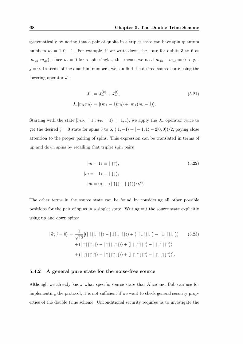
68 Chapter 5. The Double Trine Scheme
systematically by noting that a pair of qubits in a triplet state can have spin quantum
numbers m = 1, 0,−1. For example, if we write down the state for qubits 3 to 6 as
|m45,m36〉, since m = 0 for a spin singlet, this means we need m45 + m36 = 0 to get
j = 0. In terms of the quantum numbers, we can find the desired source state using the
lowering operator J−:
J− = J(k)− + J
(l)− , (5.21)
J−|mkml〉 = |(mk − 1)ml〉+ |mk(ml − 1)〉.
Starting with the state |m45 = 1,m36 = 1〉 = |1, 1〉, we apply the J− operator twice to
get the desired j = 0 state for spins 3 to 6, (|1,−1〉+ | − 1, 1〉 − 2|0, 0〉)/2, paying close
attention to the proper pairing of spins. This expression can be translated in terms of
up and down spins by recalling that triplet spin pairs
|m = 1〉 ≡ | ↑↑〉, (5.22)
|m = −1〉 ≡ | ↓↓〉,
|m = 0〉 ≡ (| ↑↓〉+ | ↓↑〉)/√
2.
The other terms in the source state can be found by considering all other possible
positions for the pair of spins in a singlet state. Writing out the source state explicitly
using up and down spins:
|Ψ; j = 0〉 =1√12
[(| ↑↓↓↑↑↓〉 − | ↓↑↓↑↑↓〉) + (| ↑↓↑↓↓↑〉 − | ↓↑↑↓↓↑〉) (5.23)
+ (| ↑↑↓↑↓↓〉 − | ↑↑↓↓↑↓〉) + (| ↓↓↑↑↓↑〉 − | ↓↓↑↓↑↑〉)
+ (| ↓↑↑↑↓↑〉 − | ↑↓↑↑↓↓〉) + (| ↑↓↑↓↑↑〉 − | ↑↓↓↑↓↑〉)].
5.4.2 A general pure state for the noise-free source
Although we already know what specific source state that Alice and Bob can use for
implementing the protocol, it is not sufficient if we want to check general security prop-
erties of the double trine scheme. Unconditional security requires us to investigate the

5.4. An Effective Quantum Channel between Alice and Bob 69
most general form of the source that is compatible with the scheme, since we are allowing
Eve to have full control of the device that distributes the qubits to Alice and Bob.
For simplicity, we continue looking for a pure state but this time we drop the con-
dition for the total spin. Although it is highly likely that the most general source state
will be a mixed state, we restrict ourselves to pure states on the pragmatic assumption
that Eve gains no clear advantage in utilizing a mixture for the source. (Recall that
a mixed state is associated with a quantum system that can be found in one of many
states in an ensemble; hence, it is somewhat more difficult to distinguish states in a
mixed state than in pure one.)
To find this state, we have seen that it is advantageous to define some new states:
|u1〉 = | ↑↓↓〉, |u2〉 = | ↓↑↓〉, |u3〉 = | ↓↓↑〉, (5.24)
|d1〉 = | ↓↑↑〉, |d3〉 = | ↑↓↑〉, |d3〉 = | ↑↑↓〉,
The definition is quite straightforward: u refers to spin-up while d refers to spin-down
and the index refers to the position of the spin in the trio which differs from the other
two. This leads to the a- and b-states being denoted by
|a1〉 =1√2
(|d3〉 − |d2〉) , |a2〉 =1√2
(|d1〉 − |d3〉) , |a3〉 =1√2
(|d2〉 − |d1〉) , (5.25)
|b1〉 =1√2
(|u3〉 − |u2〉) , |b2〉 =1√2
(|u1〉 − |u3〉) , |b3〉 =1√2
(|u2〉 − |u1〉) .
In constructing the general pure state |Ψgen〉, we first construct the j = 1/2 states
for Alice and Bob and then impose the probability conditions of the scheme (for the
noiseless channel):
prob(i, j) = tr{PiQj |Ψgen〉〈Ψgen|} =16(1− δij) for i, j = 1, 2, 3.
The construction of the j = 1/2 double trine states is greatly facilitated by looking

70 Chapter 5. The Double Trine Scheme
closely at this pair of states:
|d2〉+ |d3〉+ |d1〉√3
(j = 3/2, m = 1/2), (5.26)
|u2〉+ |u3〉+ |u1〉√3
(j = 3/2,m = −1/2).
These two vectors reside in a subspace orthogonal to the double trine subspace so what
we want are kets orthogonal to this pair.2 For j = 1/2,m = 1/2, we can have
| ⇑1〉 =|d2〉+ |d3〉q + |d1〉q2
√3
, (5.27)
| ⇑2〉 =|d2〉+ |d3〉q2 + |d1〉q√
3,
while for j = 1/2,m = −1/2, we can have
| ⇓1〉 =|u2〉+ |u3〉q + |u1〉q2
√3
, (5.28)
| ⇓2〉 =|u2〉+ |u3〉q2 + |u1〉q√
3.
The quantity q that appears in the states above is the complex phase q = exp(i2π/3).
One may also keep to real coefficients, where using the following states is equally good:
| ⇑1〉 =|d2〉 − |d1〉√
3, (5.29)
| ⇑2〉 =|d2〉 − 2|d3〉+ |d1〉√
3,
| ⇓1〉 =|u2〉 − |u1〉√
3,
| ⇓2〉 =|u2〉 − 2|u3〉+ |u1〉√
3.
2It might be worth noting that the states of (5.27)-(5.28) are related to the |ui〉 and |dj〉 by a discreteFourier transform, also known as the quantum Fourier transform in some contexts.

5.4. An Effective Quantum Channel between Alice and Bob 71
To make the notation simpler we make the following definitions:
X =
x11 x12
x21 x22
, (5.30)
[⇑⇓] =
| ⇑1⇓1〉 | ⇑1⇓2〉| ⇑2⇓1〉 | ⇑2⇓2〉
,
X ⊕ [⇑⇓] = | ⇑1⇓1〉x11 + | ⇑1⇓2〉x12 + | ⇑2⇓1〉x21 + | ⇑2⇓2〉x22.
The above definitions allow us to write the general pure state3 as
|Ψgen〉 = W ⊕ [⇑⇓] + X ⊕ [⇓⇑] + Y ⊕ [⇑⇑] + Z ⊕ [⇓⇓] .
All that remains is to find the coefficients written as elements of the matrices W ,X,Y ,
and Z.
The reader may find it useful to know the following inner products:
〈a1| ⇑1〉 = 〈b1| ⇓1〉 =(q − 1)√
6, (5.31)
〈a2| ⇑1〉 = 〈b2| ⇓1〉 =(q2 − q)√
6,
〈a3| ⇑1〉 = 〈b3| ⇓1〉 =(1− q2)√
6,
〈a1| ⇑2〉 = 〈b1| ⇓2〉 =(q2 − 1)√
6,
〈a2| ⇑2〉 = 〈b2| ⇓2〉 =(q − q2)√
6,
〈a3| ⇑2〉 = 〈b3| ⇓2〉 =(1− q)√
6,
〈ai| ⇓j〉 = 〈bi| ⇑j〉 = 0 for i = 1, 2; j = 1, 2, 3.
Those who prefer to utilize the [⇑,⇓]-states with real coefficients will get the following
3Note that this is restricted to the j = 1/2 sector for both Alice and Bob

72 Chapter 5. The Double Trine Scheme
inner products for the particular choice in Eq. (5.29):
〈a1| ⇑1〉 = 〈b1| ⇓1〉 =−1√
6, (5.32)
〈a2| ⇑1〉 = 〈b2| ⇓1〉 =−3√
6,
〈a3| ⇑1〉 = 〈b3| ⇓1〉 =−1√
6,
〈a1| ⇑2〉 = 〈b1| ⇓2〉 =2√6,
〈a2| ⇑2〉 = 〈b2| ⇓2〉 =2√6,
〈a3| ⇑2〉 = 〈b3| ⇓2〉 = 0,
〈ai| ⇓j〉 = 〈bi| ⇑j〉 = 0, for i = 1, 2; j = 1, 2, 3
What we obtain after imposing the probabilities is
|Ψgen〉 = (| ⇑2⇓1〉 − | ⇑1⇓2〉) C1 + (| ⇓2⇑1〉 − | ⇓1⇑2〉) C2 (5.33)
+ (| ⇑2⇑1〉 − | ⇑1⇑2〉) C3 + (| ⇓2⇓1〉 − | ⇓1⇓2⇓〉) C4
where
|C1|2 + |C2|2 + |C3|2 + |C4|2 =12.
for a properly normalized state.
To make more explicit the number of arbitrary real parameters we can use the
following parametrization:
C1 =
√12
cosα (5.34)
C2 = eiφ
√12
sinα cosβ
C3 = eiθ
√12
sinα sinβ cos γ
C4 = eiδ
√12
sinα sinβ sin γ
where it is clear that the arbitrary parameters are the angles {α, β, γ, δ, θ, φ}.

Bibliography
[1] S. Bartlett, T. Rudolph, R. Spekkens, Phys. Rev. Lett. 91 (2003) 027901.
[2] S. Bartlett, T. Rudolph, R. Spekkens, Rev. Mod. Phys. 79 (2007) 555-609.
[3] M. Schlosshauer, Rev. Mod. Phys. 76 (2004) 1267-1305.
[4] E. Knill, R. Laflamme, L. Viola, Phys. Rev. Lett. 84 (2000) 2525-2528.
[5] P. Zanardi, M. Rasetti, Phys. Rev. Lett. 79 (1997) 3306-3309.
[6] J. Suzuki, G. Tabia, B.-G. Englert, Phys. Rev. A 78 (2008) 052328.
73


Chapter 6
General Security Analysis
The simplest description of a cryptographic scheme, whether classical or quantum, in-
volves an ideal situation of perfect transmission between the communicating parties. In
the real world, noise is always present, and therefore, a protocol can only claim to be
secure if it can be implemented even when errors are inevitable. Techniques for coding
information are used to construct particular assemblies of information that correct for
errors automatically—these are called error correcting codes.
Unconditional security is established when, up to a certain level of noise in the chan-
nel, the scheme can still be used to privately transmit some finite amount of information.
In an information-theoretic setting, this involves a broadcast channel with two receivers
where one party is meant to receive confidential messages. A theorem by Csiszar and
Korner tells us the conditions for distilling a secure key when a classical channel is used.
For a scheme involving a quantum channel with one-way public communications, we
evaluate the C-K yield by invoking an additional theorem on the accessible information
in a quantum channel, involving a quantity called the Holevo bound. Once the error
threshold and its corresponding secure information rate are established, the remaining
task is to find an error-correcting code for producing the key. Fortunately, a coding
theorem for attaining the ultimate distillable key rate using quantum states was proven
by Devetak and Winter [1]. In this chapter, we perform a general security analysis on
the double trine scheme. The methodology here loosely follows the analysis for raw-data
attacks in BB84 [2] and for the Singapore protocol [3].
75

76 Chapter 6. General Security Analysis
6.1 Equivalent Formalism with Signal-Idler Qubits
In the previous chapter, we found a general expression for the pure state that can be used
to distribute the qubits to Alice and Bobwho communicate by using the double trine
scheme. To establish unconditional security, we calculate the bound on the accessible
information subject to the optimal measurement that Eve can perform on her ancillas
in her quest to discriminate the double trine states—the HSW bound for the source
characterized by |Ψgen〉 in Eq. (5.33).
Using the six-qubit source state above can make calculations rather tedious, espe-
cially when noise is introduced into the system. Fortunately, the properties of the above
scheme can be equivalently described in a much simpler manner by an abstract four-
qubit system, where two of the qubits are used in key generation while the other two
carry no useful information and remain unused [4]. An alternative formalism is possible
since we discover that there are in fact only four particular combinations of j = 1/2
states that are relevant in the scheme, which suggests that we only need four states in
any suitable basis. To illustrate this, let us define
| ⇑1〉 = | −+〉, (6.1)
| ⇑2〉 = |+ +〉,
| ⇓1〉 = | − −〉,
| ⇓2〉 = |+−〉.
One can think of |+〉 and |−〉 as states of any two-level system. The key to simplification
lies in the assignment of qubits. If we arrange things so that the first and third positions
are given to Alice and the 2nd and 4th positions are given to Bob, then we can rewrite
the general pure source state (5.33) as the four-qubit state:
|Ψgen〉 =(|+−+−〉 − | −+ +−〉)C1 +
(|+−−+〉 − | −+−+〉)C2
+(|+−+ +〉 − | −+ + +〉)C3 +
(|+−−−〉 − | −+−−〉)C4 (6.2)
=√
2(|S12 +−〉C1 + |S12 −+〉C2 + |S12 + +〉C3 + |S12 −−〉C4
),

6.1. Equivalent Formalism with Signal-Idler Qubits 77
where S12 refers to a singlet in the first two positions. In fact, we can rewrite the source
as,
|Ψgen〉 = |S12〉|φ34〉, (6.3)
where |φ34〉 can be any two-qubit state and is specified by a particular choice of the
coefficients C1, C2, C3, C4. In this form, it becomes readily apparent that any special
properties of the scheme can only be embodied in the first two qubits since the qubits at
positions 3 and 4 can be anything. This is reminiscent of experimentally realized qubits
using photon polarizations, where there are the qubits that carry the useful information
called signal qubits, and there are some extra qubits that play no significant role in
practical implementations called idler qubits. This can be made more explicit if we
observe the effect of the projectors for the |ai〉 and |bi〉 states. First, we define the
projectors for the double trine:
S1 =14
(1− ~σ(2) · ~σ(3)
)=
(|a1〉〈a1|+ |b1〉〈b1|), (6.4)
S2 =14
(1− ~σ(3) · ~σ(1)
)=
(|a2〉〈a2|+ |b2〉〈b2|),
S3 =14
(1− ~σ(1) · ~σ(2)
)=
(|a3〉〈a3|+ |b3〉〈b3|).
Let us examine how these projectors affect the | ⇑〉 and | ⇓〉 states:
S1|+ +〉 =23(|a1〉〈a1| ⇑2〉+ |b1〉〈b1| ⇑2〉
)(6.5)
=23
(q2 − 1)√6
[| ⇑1〉
(q2 − 1
)√
6+ | ⇑2〉(q − 1)√
6
]
=13
(|+ +〉 − | −+〉q2),
S1|+−〉 =13
(|+−〉 − | − −〉q2),
S1| − ±〉 =13
(−|+±〉q + | − ±〉) .
Notice how the second qubit is not affected by the S1 projector. Hence, we may call
this alternative formulation the signal-idler formalism for the double trine scheme.

78 Chapter 6. General Security Analysis
To further simplify matters, we may drop any references to the second qubit and write:
S1|+〉 =12
(|+〉 − |−〉q2), (6.6)
S1|−〉 =12
(−|+〉q + |−〉) .
We complete the list by including the result for the remaining projectors:
S2|+〉 =12
(|+〉 − |−〉) , (6.7)
S2|−〉 =12
(−|+〉+ |−〉) ,
S3|+〉 =12
(|+〉 − |−〉q) ,
S3|−〉 =12
(−|+〉q2 + |−〉) .
Since two quantum states are defined up to an overall phase factor (of which q =
exp(i2π/3) is an example), we can rewrite the results above as 1
Sj |j〉 = |j〉, j = 1, 2, 3, (6.8)
|j〉 = |+〉qj+1 − |−〉q−j−1,
where these newly defined j-states are, not surprisingly, vectors belonging to a trine.
Accordingly, they possess the following properties:
∑
j
|j〉 = 0 (6.9)
〈j|k〉 = 3δjk − 1. (6.10)
Expressing everything in terms of the j-states greatly simplify many of our subsequent
calculations.
1Since it is also completely arbitrary which is the first, second, or third state in a trine, we cansimplify further by choosing the Sj projectors and the j-states such that
|j〉 = |+〉qj − |−〉q−j .
In any case, the properties that come after remain unaffected whichever definition is selected.

6.1. Equivalent Formalism with Signal-Idler Qubits 79
In this language, a general qubit state is expressed as
|Q〉 =∑
j
|j〉ψj (6.11)
where we can choose∑
j
ψj = 0
so that
Sj |Q〉 = |j〉ψj . (6.12)
We can write down states for qubit pairs as well, so a two-qubit state appears as
|Q1Q2〉 =∑
j,k
|jk〉ψjk, (6.13)
where this time we impose the conditions
∑
j
ψjk =∑
k
ψjk = 0.
In order to distinguish between the double trine projectors acting on the first and second
qubit, we label them as Ai and Bi, respectively.2 We can then write down the relation
AjBk|Q1Q2〉 = |jk〉ψjk.
As a final remark to this section, it is worth mentioning that the general qubit state
given here corresponds exactly to an RFF-qubit for the double trine scheme. To see the
connection, we list down the Pauli vectors associated with the signal-idler qubits:
σ(SIQ)X =
23
[14~σ(3) · ~σ(1) − 1
8(~σ(2) · ~σ(3) + ~σ(1) · ~σ(2)
)], (6.14)
σ(SIQ)Y =
14√
3
(~σ(1) · ~σ(2) − ~σ(2) · ~σ(3)
),
σ(SIQ)Z =
16√
3
[(~σ(2) × ~σ(1)) · ~σ(3) + (~σ(1) × ~σ(3)) · ~σ(2) + (~σ(3) × ~σ(2)) · ~σ(1)
].
2This means that Si = Ai = Bi. Here the labels are conveniently chosen so that one can easilyassociate the double trine operators to Alice and Bob.

80 Chapter 6. General Security Analysis
We can check that these components of ~σ(SIQ) are rotationally invariant and that they
obey the usual properties for Pauli operators:
tr{σ(SIQ)k } = 0, (6.15)
σ(SIQ)i σ
(SIQ)j = δij + iεijkσ
(SIQ)k , for i, j, k = X, Y, Z.
6.2 Source with Eve’s Ancilla States
Having established a simplifying formalism, we apply this to the security analysis of the
double trine scheme by letting Eve entangle her ancilla states with the two-qubit state
that Alice and Bob receives. In this situation the source state is given by
|S〉 =∑
j,k
|jkEjk〉, (6.16)
where |j〉 is received by Alice, |k〉 is received by Bob, and |Ejk〉 refer to Eve’s ancilla.
Eve’s task remains the same as in any protocol: to maximize her mutual information
with Alice (or Bob, depending on whom she eavesdrops). For every such state that Eve
sends, there is a corresponding optimal POVM that will maximize her information.
The actual appearance of the POVM elements depend on several adjustable parameters
determined by observing that insisting on a source state with the structure given above
is equivalent to constraints imposed by expected probabilities of measurement outcomes
by Alice and Bob. To measure the state of the qubits, Alice and Bob use suitable
POVMs composed of the Aj projectors we described in a previous section. Note that
∑
j
Aj = 1 (6.17)
Aj |Q〉 = |j〉ψj ,
which are exactly the properties we need for elements of a POVM. When Alice and Bob
apply their POVM operators, the result is
AjBk|S〉 = |jkEjk〉.

6.2. Source with Eve’s Ancilla States 81
Naturally we have the probability conditions:
pjk = 〈S|AjBk|S〉 = 4〈Ejk|Ejk〉 (6.18)
= (1− ε)16(1− δjk) +
ε
9.
To choose the parameters for Eve’s ancillas, we can express |Ejk〉 in a relatively sym-
metric fashion with
|Ejk〉 =19
[|E1〉q−j−k + |E2〉q−j+k + |E3〉qj−k + |E4〉qj+k
].
Obtaining a set of ancillas that provide Eve the most knowledge about Alice and Bob’s
qubits requires finding the |Ei〉 states which satisfy
V =(|E1〉 |E2〉 |E3〉 |E4〉
), (6.19)
V †V =14
1 + a + b + c u v 0
u∗ 1 + a− b− c −2(1− ε) −v
v∗ −2(1− ε) 1− a + b− c −u
0 −v∗ −u∗ 1− a− b + c
for a, b, c ∈ R and u, v ∈ C. The matrix V †V is nothing more than constraints imposed
by the probabilities pjk on the inner products between the |Ei〉 states.
Taking the simplest case of u = v = 0, positivity of the above matrix requires
a = b = 0. Thus the resulting matrix is
M =14
1 + c 0 0 0
0 1− c −2(1− ε) 0
0 −2(1− ε) 1− c 0
0 0 0 1 + c
.
If we factorize this matrix M as V T V so it automatically fulfills the positivity condition,

82 Chapter 6. General Security Analysis
we obtain
V =12
√1 + c 0 0 0
0 x y 0
0 y x 0
0 0 0√
1 + c
=(|E1〉 |E2〉 |E3〉 |E4〉
), (6.20)
where
x2 + y2 = 1− c, −1 ≤ c ≤ 2ε− 1 (6.21)
2xy = −2(1− ε).
Thus, Eve’s ancilla states are composed of the kets
|Ejk〉= 118
√1 + cq−j−k
xq−j+k + yqj−k
xqj−k + yq−j+k
√1 + cqj+k
. (6.22)
We can now calculate brackets of these |Ejk〉 states. All relevant brackets can be obtained
from the following set, noting that (j, k, l) can be any permutation of (1, 2, 3).
〈Ekj |Ekj〉 =3− ε
162, 〈Ekj |Elj〉 =
−3 + 2ε162
,
〈Ekj |Ekk〉 =−ε
162, 〈Ekj |Elk〉 =
3− 3c− 2ε
324,
〈Ekj |Ekl〉 =−3 + 2ε
162, 〈Ekj |Ell〉 =
3 + 3c− 2ε
324,
〈Ekj |Ejk〉 =−3 + 3c + 4ε
324, 〈Ekj |Ejj〉 =
−ε
162,
〈Ekj |Ejl〉 =3− 3c− 2ε
324, 〈Ekk|Ejj〉 =
−3− 3c + 4ε
324,
〈Ekk|Ekk〉 =ε
81.
Eve can choose whether she wants to eavesdrop on Alice or Bob. Because of the
asymmetric nature of the scheme, the resulting conditioned ancilla states will be differ-
ent. We also consider the bit case and trit case independently since these are mutually

6.2. Source with Eve’s Ancilla States 83
exclusive events. If Eve eavesdrops on Alice, the unnormalized conditioned ancillas for
the bit case are
ρ(A)jk = |EkjElk〉〈EkjElk|+ |EljEjk〉〈EljEjk|+ |EkjEjk〉〈EkjEjk|
+|EkkElj〉〈EkkElj |+ |ElkEjj〉〈ElkEjj |+ |EkkEjj〉〈EkkEjj |, (6.23)
ρ(A)kj = |EjkEkj〉〈EjkEkj |+ |ElkEjk〉〈ElkEjk|+ |EjkElj〉〈EjkElj |
+|EljEkk〉〈EljEkk|+ |EjjElk〉〈EjjElk|+ |EjjEkk〉〈EjjEkk|,
where j and k refer to any 2 distinct elements taken from the set of outcomes {A,B, C},the subscripts jk and kj referring to the possible bit results, and the superscript A
telling us the density operators are conditioned on Alice.
To get an idea how these states were obtained, let us look at the first term of ρ(A)jk :
each |Ejk〉 refers to a pair of measurement outcomes, the first index belonging to Alice
and the second one to Bob. So Alice’s pair is (k, l) while Bob’s is (j, k). Bob has different
states so this is a bit case and they will agree on (j, k). For the trit case, we have
ρ(A)j = |EkjElj〉〈EkjElj |+ |EljEkj〉〈EljEkj |+ |EkkElk〉〈EkkElk|
+|ElkEkk〉〈ElkEkk|+ |EklEll〉〈EklEll|+ |EllEkl〉〈EllEkl|, (6.24)
ρ(A)k = |EjkElk〉〈EjkElk|+ |ElkEjk〉〈ElkEjk|+ |EjjElj〉〈EjjElj |
+|EljEjj〉〈EljEjj |+ |EjlEll〉〈EjlEll|+ |EllEjl〉〈EllEjl|,
ρ(A)l = |EjlEkl〉〈EjlEkl|+ |EklEjl〉〈EklEjl|+ |EjjEkj〉〈EjjEkj |
+|EkjEjj〉〈EkjEjj |+ |EjkEkk〉〈EjkEkk|+ |EkkEjk〉〈EkkEjk|.
On the other hand, if Eve eavesdrop on Bob, she gets the following ancilla states for the

84 Chapter 6. General Security Analysis
bit case
ρ(B)jk = |EkjElk〉〈EkjElk|+ |EljEjk〉〈EljEjk|+ |EkjEjk〉〈EkjEjk| (6.25)
+|EljEkk〉〈EljEkk|+ |EjjElk〉〈EjjElk|+ |EjjEkk〉〈EjjEkk|,
ρ(B)kj = |EjkEkj〉〈EjkEkj |+ |ElkEjk〉〈ElkEjk|+ |EjkElj〉〈EjkElj |
+|EkkElj〉〈EkkElj |+ |ElkEjj〉〈ElkEjj |+ |EkkEjj〉〈EkkEjj |,
as well as for the trit case
ρ(B)j = |EkjElj〉〈EkjElj |+ |EljEkj〉〈EljEkj |+ |EjjElj〉〈EjjElj | (6.26)
+|EljEjj〉〈EljEjj |+ |EjjEkj〉〈EjjEkj |+ |EkjEjj〉〈EkjEjj |,
ρ(B)k = |EjkElk〉〈EjkElk|+ |ElkEjk〉〈ElkEjk|+ |EkkElk〉〈EkkElk|
+|ElkEkk〉〈ElkEkk|+ |EjkEkk〉〈EjkEkk|+ |EkkEjk〉〈EkkEjk|,
ρ(B)l = |EjlEkl〉〈EjlEkl|+ |EklEjl〉〈EklEjl|+ |EklEll〉〈EklEll|
+|EllEkl〉〈EllEkl|+ |EjlEll〉〈EjlEll|+ |EllEjl〉〈EllEjl|.
One may notice that the conditioned ancilla states for Alice and Bob differ only on the
terms that contribute errors to the key generation process. Thus, we explore both sets
of ancillas, to see whether Eve gains any advantage by eavesdropping on either Alice
or Bob, or if it does not make any difference to the optimal amount of information she
can obtain. By construction∑j,k
|Ejk〉 = 0.(This is also a consequence of the fact that
we define our states using a linearly dependent set). This gives us the following useful
relations:
|EkjElk〉+ |EjjElk〉 − |EljEkk〉 − |EljEjk〉 = 0, (6.27)
|EkjElk〉+ |EkjEjk〉 − |EjjElk〉 − |EjjEkk〉 = 0,
|ElkEkj〉+ |ElkEjj〉 − |EkkElj〉 − |EjkElj〉 = 0,
|EkkEjj〉+ |EkkElj〉 − |ElkEkj〉 − |EjkEkj〉 = 0.

6.3. Finding the Optimum Information Bound on Eve’s Ancillas 85
6.3 Finding the Optimum Information Bound on Eve’s
Ancillas
Ultimately, we are interested in finding the maximum amount of information that Eve
can obtain by eavesdropping on Alice or Bob. From the previous section we recall that
Eve’s states |Ei〉 in general depend on seven real parameters. We wish to find the values
of these parameters such that Eve gets as much information about the measurement out-
comes as possible. First, we treat the optimization problem with a single free parameter.
The ancilla states for Eve are given by Eq. (6.22).
In this section, it will be convenient to define the following constants:
a =3− ε
162, b =
−ε
162,
c =−3 + 2ε
162, d =
3− 3α− 2ε
324,
e =3 + 3α− 2ε
324, f =
−3 + 3α + 4ε
324,
g =−3− 3α + 4ε
324, h =
ε
81.
These numbers comprise the set of all possible values for the inner products among
the |Ejk〉 in the one-parameter case, where α is the floating parameter. You can check
this by solving the 81 relevant inner products using Eq. (6.22). We can then form
the matrix of brackets from which we deduce a suitable representation of Eve’s ancilla
states. Firstly, we obtain the following set of submatrices Bi (the label refers to the bit
case):
B1 =
a2 c2 ac
c2 a2 ca
ac ca a2
, B2 =
ha b2 hb
b2 ah bh
hb bh h2
, B3 =
bc de be
ed cb eb
bd db b2
,
B4 =
fc d2 fd
d2 cf df
fd df f2
, B5 =
ba cb b2
bc ab b2
bc cb b2
, B6 =
cg e2 ge
e2 cg eg
ge eg g2
.
(6.28)

86 Chapter 6. General Security Analysis
which forms the larger matrix of brackets when arranged as
B =
B1 B3 B4 BT5
BT3 B2 B5 B6
B4 BT5 B1 B3
B5 B6 BT3 B2
. (6.29)
The same thing should be done for the trit case:
T =
T11 T T21 T T
31 T T41 T T
51 T T61
T21 T22 T T32 T T
42 T T52 T T
62
T31 T32 T33 T T43 T T
53 T T63
T41 T42 T43 T44 T T54 T T
64
T51 T52 T53 T54 T55 T T65
T61 T62 T63 T64 T65 T66
.
where the elements of T are giving in Eq. (6.30) at the end of this section. Recall
that our objective here is to factorize this matrix of brackets in order to get a matrix
of ancilla states, which we will need to compute the Holevo-Schumacher-Westmoreland
(HSW) bound on the accessible information.
There are a few other things we can consider to help simplify our work. First, let’s
look at certain relations among the various parameters characterizing the elements of
B. Using the constants given above, the following equations should be easy to verify:
a + b + c = 0, c + d + e = 0,
2b + h = 0, b + d + f = 0,
b + g + e = 0.
As a consequence, these equations allow us to determine eigencolumns with eigenvalue
zero for B (and hence, deduce the number of dimensions in which the ancilla states
reside). With the help of∑j,k
|Ejk〉 = 0 and its accompanying relations (6.28), we find

6.3. Finding the Optimum Information Bound on Eve’s Ancillas 87
the following eigencolumns of eigenvalue zero:
(1,−1, 0, 0, 0, 0, 0, 0, 0, 1,−1, 0)T ,(0, 1, 1, 0, 0, 0, 0, 0, 0,−1, 0,−1)T ,
(0, 0, 0,−1, 1, 0,−1, 1, 0, 0, 0, 0)T ,(1,−1, 0, 0, 0, 0, 0, 0, 0, 1,−1, 0)T .
This implies that the subspace for {|Ejk〉} must be at most eight-dimensional.3
As promised earlier, we end the section by listing the elements of T :
T11 =
a2 bc bc
bc ah b2
bc b2 ah
, T21 =
fc ba db
ba gc eb
db eb ch
, T22 =
a2 bc cb
bc ah b2
cb b2 ah
,
T31 =
d2 ef cb
bc gd e2
fe b2 dg
, T32 =
cf bd ab
bd hc be
ab be cg
, T33 =
a2 bc cb
bc ha b2
cc b2 ah
,
T41 =
c2 ed de
de b2 fg
ed gf b2
, T42 =
d2 bc fe
cb e2 dg
ef gd b2
, T43 =
fc ba db
db eb ch
ba gc eb
,
T44 =
a2 bc bc
bc ah b2
bc b2 ah
, T51 =
d2 bc fe
cb e2 dg
ef gd b2
, T52 =
c2 ed de
de b2 fg
ed gf b2
,
T53 =
d2 ef cb
fb b2 dg
bc gd e2
, T54 =
fc ba db
ba gc eb
db eb ch
, T55 =
a2 bc cb
bc ha b2
cb b2 ah
,
T61 =
cf bd ab
ab be cg
bd hc be
, T62 =
d2 ef cb
fe b2 dg
bc gd e2
, T63 =
c2 ed de
de b2 fg
ed gf b2
,
T64 =
d2 ef cb
bc gd e2
fe b2 dg
, T65 =
cf bd ab
bc hc be
ab be cg
, T66 =
a2 bc cb
bc ha b2
cb b2 ah
.
(6.30)
3This can be used as a check on the numerical results we obtain later.

88 Chapter 6. General Security Analysis
6.4 Numerical Results for the One-Parameter Optimiza-
tion
We have opted to first try the special case of a single parameter since it is the simplest
problem we can try to solve as well as it may be amenable to a full analytical solution.
Unfortunately, the purely analytical result for finding the optimal parameter values
remains elusive despite many efforts in simplification. Nonetheless, all our previous
results can still be used to verify the numerical solutions we have obtained.
The numerical optimization was performed using a simple MATLAB code.4 (Some
of the results have been double-checked using the SOMIM program [5], which uses a
more efficient algorithm than the direct optimization method done here.) After the
optimum is found, we can plot the accessible information and find the C-K yield for the
double trine scheme. The relevant plots for ancillas conditioned on Alice and Bob are
presented in Fig.(6.1) for the bit case and Fig.(6.2) for the trit case.
At first glance, the results reveal one rather troubling aspect: the amount of in-
formation that Eve gets if she eavesdrop on Alice is different from what she gets if she
eavesdrops on Bob. This is a curious finding: intuitively, you would expect that Eve gets
precisely the same amount of information from either because Alice and Bob’s qubits
should carry the same information if they are to agree on a key. This is indeed the
case if the channel were perfect but it is false when noise is present. The discrepancy
originates from the error terms in the conditioned states, and in some sense you could
say that Alice’s states are less informative to Eve when it comes to figuring out the key.
What the results reflect is a genuine asymmetry in the key generation process between
Alice and Bob. Although Alice and Bob have the same information for producing the
key, the information available to Eve for a particular choice of {|Ei〉} is vastly different.
In the single parameter case, we see that Eve would choose to eavesdrop on Bob since
she gets more information for the same level of noise.
4The MATLAB codes are available in the Appendix of this thesis.

6.4. Numerical Results for the One-Parameter Optimization 89
0 0.2 0.4 0.6 0.8 10
0.1
0.2
0.3
0.4
0.5
0.6
0.7
0.8
0.9
1
noise parameter
mut
ual i
nfor
mat
ion
I(A:B)I(A:E)I(B:E)
Figure 6.1: One-parameter case: Wiretapper bound for Eve during a bit case. For Alice,the error threshold is ε = 0.196 corresponding to a C-K yield of IC−K = 0.561. Thecorresponding numbers for Bob are ε = 0.170, IC−K = 0.604.
0 0.2 0.4 0.6 0.8 10
0.5
1
1.5
noise parameter
mut
ual i
nfor
mat
ion
I(A:B)I(A:E)I(B:E)
Figure 6.2: One-parameter case: Wiretapper bound for Eve during a trit case.For Alice,the error threshold is ε = 0.193 corresponding to a C-K yield of IC−K = 0.619. Thecorresponding numbers for Bob are ε = 0.150, IC−K = 0.744

90 Chapter 6. General Security Analysis
6.5 Asymmetry between Alice’s and Bob’s Conditioned
Ancillas
The numerical results for the computation of the Holevo bound indicate a glaring asym-
metry between Alice and Bob. In both bit and trit cases, the numbers indicate a higher
error threshold for Alice, meaning that it is more advantageous for Eve to eavesdrop on
Alice at all times. This situation is quite perplexing because after the key is generated,
we expect both versions of the key to contain exactly the same information. But it could
be that this is not a real asymmetry. We note that the numerical computation uses a
particular input ancilla state for Alice and Bob. It is still possible that given a different
ancilla state, it would be more useful for Eve to look at Bob’s data. Furthermore, what
would be interesting to show is that there is another set of Eve’s states that simply
reverses the roles of Alice and Eve in the numerical analysis. To address all this issues,
we have to optimize for all free parameters.
We recall that one symmetric parametrization of Eve’s ancillas is given by
|Ejk〉 =19
[|E1〉q−j−k + |E2〉q−j+k + |E3〉qj−k + |E4〉qj+k
],
where we can obtain the appropriate |Ei〉 states from the condition
M = V T V =
〈E1|〈E2|〈E3|〈E4|
(|E1〉 |E2〉 |E3〉 |E4〉
), (6.31)
where V and |Ei〉 are defined in Eq. (6.20). In this language, a different set of |Ei〉corresponds to a different choice of the parameters a, b, c, u, and v.
In general, we observe that the analysis is greatly facilitated by choosing a suitable
parameterization of V that has a simple and manageable mathematical structure. It
aids us a lot if we recall the following properties of the matrix M and the vectors |Ei〉 :

6.5. Asymmetry between Alice’s and Bob’s Conditioned Ancillas 91
• 1. It is positive, hermitian, and of unit trace.
• 2. 〈E1|E4〉 = 〈E4|E1〉 = 0.
• 3. 〈E2|E3〉 = 〈E3|E2〉 = −(1− ε)/2.
• 4. 〈E1|E2〉+ 〈E3|E4〉 = 〈E2|E1〉+ 〈E4|E3〉 = 0.
• 5. 〈E1|E3〉+ 〈E2|E4〉〈E3|E1〉+ 〈E4|E2〉 = 0.
One possible choice for the vectors |Ei〉 is given by the columns of the following
matrix:
V =12
a1 λa4 −µa4 0
0 r1 cos(θ) −r2eiφ sin(θ) 0
0 r2eiφ sin(θ) −r2 cos(θ) 0
0 µ∗a1 −λ∗a1 a4
(6.32)
In this basis for Eve’s ancilla qubits, the matrix E appears as
M = V T V =14
a21 λa1a4 −µa1a4 0
λ∗a1a4 P R µa1a4
−µ∗a1a4 R Q −λa1a4
0 µ∗a1a4 −λ∗a1a4 a24
(6.33)
where
P = r21 + |µ|2a2
1 + |λ|2a24, (6.34)
Q = r22 + |µ|2a2
4 + |λ|2a21,
R = −2(1− ε).
There are two more constraints on the set of parameters a1, a4, r1, r2, λ, µ, φ, namely
the condition for unit trace, and the condition relating the parameters to ε:
4 = (1 + |λ|2 + |µ|2)(a21 + a2
4) + r21 + r2
2, (6.35)
2(1− ε) = λ∗µ(a21 + a2
4) + r1r2eiφ sin(2θ).

92 Chapter 6. General Security Analysis
Note that in principle, how we decompose matrix M is not important for obtaining
the solution. However, we use the parameters above because it is more amenable to
both analytical and numerical methods of optimization.
Before we optimize for the full set of parameters, we would also like to introduce
another assumption about the ancilla states. Recall that to add a character to either the
bit key or the trit key, Alice has to choose two positions on their measurement records.
The sequence in which this positions is in fact not important: this is quite obvious in
the trit case since the letter they will add to the key is the one not appearing on either
position. For the bit case, this is less apparent but because the decision for assigning
which order is ’0’ and ’1’ is random, then it should not depend on the order the positions
are chosen. Note this condition of position order symmetry has not been shown to be
a necessary one in general but is a definitely a reasonable symmetry property for the
optimal solution. This leads to a set of constraints on the brackets of |Ejk〉:
〈Ekj |Ekj〉 = 〈Ejk|Ejk〉, 〈Ejj |Ejj〉 = 〈Ekk|Ekk〉,〈Ekj |Ekk〉 = 〈Ejk|Ejj〉, 〈Ekj |Elj〉 = 〈Ejk|Elk〉,〈Ekj |Elk〉 = 〈Ejk|Elj〉, 〈Ekk|Elj〉 = 〈Ejj |Elk〉,〈Ekk|Elk〉 = 〈Ejj |Elj〉.
(6.36)
The two conditions on the first line are in fact automatically true. To satisfy the
remaining constraints, we have to choose:
a1 = a4, µ = µ∗,
r1 = r2, λ = −λ∗,
φ = 0.
By imposing these new conditions along with the previous ones, we effectively reduce
the problem to two real parameters. The results of the C-K yield calculation appear in
Figs. (6.3)-(6.4).
Within the numerical accuracy of the program, the results obtained here coincide

6.5. Asymmetry between Alice’s and Bob’s Conditioned Ancillas 93
0 0.2 0.4 0.6 0.8 10
0.2
0.4
0.6
0.8
1
noise parameter
mut
ual i
nfor
mat
ion
I(A:B)I(A:E)I(B:E)
Figure 6.3: Optimizing with position order symmetry: Wiretapper bound for Eveeavesdropping during a bit case. For Alice, the error threshold is ε = 0.197 corre-sponding to a C-K yield of IC−K = 0.560. The corresponding numbers for Bob areε = 0.170, IC−K = 0.603
0 0.2 0.4 0.6 0.8 10
0.5
1
1.5
noise parameter
mut
ual i
nfor
mat
ion
I(A:B)I(A:E)I(B:E)
Figure 6.4: Optimizing with position order symmetry: Wiretapper bound for Eveeavesdropping during a trit case. For Alice, the error threshold is ε = 0.193 corre-sponding to a C-K yield of IC−K = 0.618. The corresponding numbers for Bob areε = 0.150, IC−K = 0.744

94 Chapter 6. General Security Analysis
precisely with the outcome of the one-parameter optimization. This is a rather aston-
ishing result. Remember that we ended up with a single parameter to optimize in the
earlier special case by simply setting some parameters to zero and imposing positivity.
Keeping all parameters free but then introducing a plausible symmetry into the |Ejk〉states, the numerical result still did not change appreciably. We suspect that, in fact,
the optimal solution for the general case is identical to the solution of the one-parameter
case. We have not proven this to be definitely true but we have strong numerical evidence
pointing to this fact.

Bibliography
[1] I. Devetak, A. Winter, Proc. R. Soc. A 461 (2005) 207-235.
[2] S.M. Assad, J. Suzuki, B.-G. Englert, Int. J. Quant. Inform. 4 (2006) 1003-1012.
[3] J. Anders, H.K. Ng, B.-G. Englert, S. Y. Looi, arxiv:quant-ph/0505069 (2005).
[4] J. Rehacek, B.-G. Englert, private communication.
[5] K. L. Lee, W. K. Chua, S. Y. Looi, B.-G. Englert, SOMIM: An
open-source program code for the numerical Search for Optimal Mea-
surements by an Iterative Method, arXiv:0805.2847 (2008). Website:
http://theory.quantumlah.org/project/SOMIM/
95


Chapter 7
Concluding Remarks
The main subject of this thesis is reference frame-free quantum key distribution using
a double trine scheme. Due to the rotationally invariant construction of the quantum
states used for distilling a secret key, the protocol is definitely basis-independent: Alice
and Bob can choose their measurement coordinates independently without worrying
about any decoherence due to mismatched bases. Of course, this provision works under
the reasonable assumption that any environmental effects that may affect the qubits in
transit affect all the qubits equally. It is not difficult to imagine that qubits traveling
along the same medium (like photons propagating inside an optical fiber) will experience
common external effects.
One curious characteristic of the key generation procedure used for the double trine
scheme is its dual alphabet. Depending on how pairs of letters between Alice and Bob
match, they may end up adding a symbol on the bit key or the trit key. Although
it seems more complicated than the single-alphabet key distillation process for trines,
which include inconclusive outcomes when Alice and Bob try to match letters, the two-
alphabet key is actually more efficient, achieving an information rate of 98% of the
channel capacity in the ideal scenario. In fact, the steps in the key distillation do not
require specific properties of double trine states, which means that the dual-alphabet
key generation can be utilized for any QKD protocol that uses trines.
Of course, the true value of a cryptographic protocol lies not only in the ease of
implementation or the efficiency in generating a key. A cryptographic scheme is most
97

98 Chapter 7. Concluding Remarks
useful if it is unconditionally secure. The previous chapter dealt with analyzing the
security of the double trine scheme using a convenient formalism with signal-idler logical
qubits. As an important special case, we first considered a single parameter optimization
problem where we set all except one of the adjustable parameters of our tomographically
incomplete protocol to zero. The single parameter is reminiscent of the free parameter
in the analysis of raw-data attacks for the BB84 scheme.
A remarkable result we obtain from the numerical calculations show that the single-
parameter solution is already an optimal solution for the full optimization problem. To
demonstrate this, we free up all the adjustable parameters but invoke an additional
plausible symmetry assumption on the conditioned ancilla states. The symmetry has to
do with the interchangeability of the order of the pairs of letters chosen by Alice. Each
symbol in the key is generated from pairs of letters from the transmitted raw data. We
observe that Alice has the freedom to choose which is the first letter of the pair and
which one is the second; this is inconsequential in producing the key. By imposing this
symmetry, we arrive at a two-parameter optimization problem, the solution reproduces
that of the special case.
We found an absolute noise threshold of ε = 0.170 for the bit case and ε = 0.15 for
the trit case, both of which are achieved by Eve only if she eavesdrops on Bob. Hence,
we see one curious implication of this result: there is a way of choosing the states such
that it is more advantageous to eavesdrop on one party. As far as we are aware of, this
is not the case for any other protocols, at least for the more popular ones like BB84 and
E91 and their variants, or for trine-based schemes like PBC00. We suspect, but have not
shown rigorously, that the asymmetry is a direct consequence of the asymmetry in the
key generation process itself: although Alice and Bob arrive at the same key in the ideal
case, they do so through using entirely different symbols from the raw data. This creates
a discrepancy in how Eve’s ancillas are conditioned: she acquires different amounts of
information from Alice and Bob for any specific source state she uses. This further
implies that the two roles in the key distillation are not completely interchangeable, in
the sense that there is no other choice of the source such that the amount of information
that Alice acquires from eavesdropping are simply reversed. Note however that once

99
Alice and Bob performs further classical post-processing tasks such as error correction
and privacy amplification, they can use Bob’s set of letters for reference to make things
more difficult for Eve.
A full optimization of the seven parameters without any other preconditions will
resolve any remaining issues. However, the task remains difficult because of the relatively
complicated dependence of the source state on the seven parameters. The primary
impediment has been in handling some of the nonlinear constraints. Such a parameter
space may still manageable using nonlinear numerical optimization techniques but it
is virtually inaccessible to analytical methods without additional assumptions being
imposed.
It will also be interesting to discuss the details of a practical implementation of the
scheme. Producing entangled states has never been an easy task, with the difficulty
increasing rapidly with size. A practical system with a common source for Alice and
Bob requires six entangled qubits for each transmission. It makes more sense to use
the variant were Alice prepares the states and sends them to Bob; this will require only
three qubits and this would be much easier to produce. As with other QKD protocls,
photon polarizations remain the most likely candidate for an actual working prototype
for preparing double trine states. It is in fact quite easy to envision and implement
the following situation: Alice prepares three-photon trine states by first producing two
of the three photons in a polarization Bell-state. The remaining photon then carries
a completely random polarization. Bob’s POVM would then tests if one of the three
orthogonal Bell-states is present for every trio of photons Alice sends him.


Appendix
MATLAB codes for calculating Holevo bounds in the one-
parameter and position-order symmetry cases
A. Main program for calculating the Holevo bound and the C-K yield
Given below is the MATLAB script file that generates the security analysis data.
The example is the one for Eve eavesdropping on Alice in a bit case and thus uses
mutualInfoAEbit. You can replace this function with mutualInfoAEtrit, mutualInfoBEbit,
and mutualInfoBEtrit to compute the C-K yield for the Alice trit case, Bob bit
case, and Bob trit case, respectively in the single-parameter optimization. For the
full optimization with position order symmetry, we use the functions searchMax and
AliceBitMutualInfo, BobBitMutualInfo, AliceTritMutualInfo, BobTritMutualInfo
to calculate optimum.
% main script file for running code
clear all
n = 10000;
u(1) = 0; v(1) = 1; y(1) = -1; w = linspace(0,1,n+1);
for j = 1:n
v(j+1) = mutualInfoABbit(j/n);
optimum = grSearchMax(’mutualInfoAEbit’,j/n,[-1 (2*(j/n)-1)], 100);
y(j+1) = optimum(1);
u(j+1) = optimum(2);
end
101

102 Appendix
x = u - v;
save optimizeAlicebit.mat
B. Cholesky decomposition of positive semi-definite matrices
MATLAB has an efficient built-in function for calculating the Cholesky decomposition of
a positive definite matrix. However, it does not work for matrices with zero eigenvalues.
Hence, the need for constructing a special code to handle our density operators. When
you have a positive semi-definite matrix M , the choice for the upper triangular matrix
U such that M = UT U is not unique. However, for the purposes of calculating the
Holevo bound, it is sufficient to choose any matrix U that works.
function U = CholeskyDecomposition(M, tol)
% This functions yields the Cholesky or triangular decomposition of
% a positive semi-definite matrix M such that M = U’*U
[m,n] = size(M);
if m ~= n
error(’M must be a square matrix’);
end
U = zeros(n); rankM = rank(M);
for i = 1:n
for j = i:n
if j == 1
s = M(i,i);
else
s = M(i,j) - U(1:i-1,i)’*U(1:i-1,j);
end
if abs(s) < tol
s = 0;
end
if j > i

Appendix 103
if abs(U(i,i)) < tol
if j == (i+1)
s = M(i+1,i+1) - U(1:i,j)’*U(1:i,j);
else
s = M(i+1,j) - U(1:i,i+1)’*U(1:i,j);
end
if abs(s) < tol
s = 0;
end
if j > (i+1)
if abs(U(i,i+1)) < tol
U(i,j) = 0;
else
U(i,j) = s/U(i,i+1);
end
else
if s < 0
error(’Cholesky matrix U is not positive definite.’);
end
U(i,i+1) = sqrt(s);
end
elseif abs(U(i,i)) > tol
U(i,j) = s/U(i,i);
end
else
if s < 0
error(’Cholesky matrix U is not positive definite.’);
end
U(i,i) = sqrt(s);
end
end
end

104 Appendix
C. Shannon entropy of density operators with known eigenvalues
Calculating eigenvalues of matrices is rather straightforward in MATLAB so the alter-
native definition of Shannon entropy in terms of eigenvalues is particularly useful here.
The only relevant condition to add is to accept only non-zero eigenvalues because the
logarithm tends to negative infinity as the eigenvalue approaches zero.
function S = entropy(eigrho)
% This function computes the Shannon entropy S for a density operator whose
% eigenvalues eigrho(i) are known.
S = 0; N = length(eigrho);
for i = 1:N
if ((eigrho(i)) > 0)
S = S - eigrho(i)*log2(eigrho(i)) ;
end
end
D. Searching for the maximum of a function using the golden ratio
method
The golden ratio search is a simple yet robust method for finding the extremum values
of a unimodal function over a given interval and successively looking at smaller range of
values. It involves dividing the said interval into two parts whose lengths give the golden
ratio. The advantage of this method compared to the bisection method is that it con-
verges faster and at a most consistent rate especially in the case when the extremum to
be found is close to any midpoint you eventually get during the progressive subdividing.
function maxVector = grSearchMax(func, eps, bounds, n)
% This function calculates the local maximum of a function using the golden
% ratio algorithm.
% func is name of function for which max is searched, string format
% bounds is a 2-vector [a b] for the interval (a,b) to be considered
% n is number of iterations

Appendix 105
phi = (1 + sqrt(5))/2; xa = bounds(1); xb = bounds(2);
fa = feval(func,eps, xa); fb= feval(func,eps, xb);
for i = 1:n
xu = xa + (xb - xa)/(1+phi);
xv = xa + (xb - xa)/(1+(1/phi));
fu = feval(func,eps, xu);
fv = feval(func,eps, xv);
if fu > fv
maxValue = fu;
maxX = xu;
xb = xv;
else
xa = xu;
maxValue = fv;
maxX = xv;
end
end
if (maxValue < feval(func,eps, bounds(1))) || (maxValue < feval(func,eps,bounds(2)))
if feval(func,eps,bounds(1)) < feval(func,eps,bounds(2))
maxValue = feval(func,eps, bounds(2));
maxX = bounds(2);
else
maxValue = feval(func,eps,bounds(1));
maxX = bounds(1);
end
end
maxVector = [maxX, maxValue];
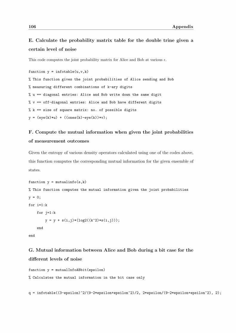
106 Appendix
E. Calculate the probability matrix table for the double trine given a
certain level of noise
This code computes the joint probability matrix for Alice and Bob at various ε.
function y = infotable(u,v,k)
% This function gives the joint probabilities of Alice sending and Bob
% measuring different combinations of k-ary digits
% u == diagonal entries: Alice and Bob write down the same digit
% v == off-diagonal entries: Alice and Bob have different digits
% k == size of square matrix: no. of possible digits
y = (eye(k)*u) + ((ones(k)-eye(k))*v);
F. Compute the mutual information when given the joint probabilities
of measurement outcomes
Given the entropy of various density operators calculated using one of the codes above,
this function computes the corresponding mutual information for the given ensemble of
states.
function y = mutualinfo(s,k)
% This function computes the mutual information given the joint probabilities
y = 0;
for i=1:k
for j=1:k
y = y + s(i,j)*(log2((k^2)*s(i,j)));
end
end
G. Mutual information between Alice and Bob during a bit case for the
different levels of noise
function y = mutualInfoABbit(epsilon)
% Calculates the mutual information in the bit case only
q = infotable((3-epsilon)^2/(9-2*epsilon+epsilon^2)/2, 2*epsilon/(9-2*epsilon+epsilon^2), 2);

Appendix 107
s = mutualinfo(q,2);
y = s;
H. Mutual information between Alice and Bob during a trit case for
the different levels of noise
function y = mutualInfoABtrit(epsilon)
% Calculates the mutual information in the trit case only
p = infotable((1/9)*((3-epsilon)/(1+epsilon)),
(1/9)*(2*epsilon/(1+epsilon)), 3);
r = mutualinfo(p,3);
y = r;
I. Accessible information between Alice/Bob and Eve during a bit/trit
case
The function that computes the Holevo bound at various ε. There are four different
functions, one for each conditioned ancilla that Eve uses when she eavesdrop on Alice
or Bob during the bit or trit case. These are mutualInfoAEbit, mutualInfoAEtrit,
mutualInfoBEbit, and mutualInfoBEtrit, where the identity of each is apparent in
the label. The bit case for Eve’s ancilla states conditioned on Alice is given in full below
and the modified parts for the other scenarios are given after it.
For mutualInfoAEbit:
function y = mutualInfoAEbit(epsilon, c)
%%%%%%%%%%%%% Ejk code %%%%%%%%%%%%%%%%%%%%%%%%
%initialize Ejk states
a = 0; b = 0; u = 0; v = 0;
A = (1/4)*[ (1+a+b+c) u v 0;
conj(u) (1+a-b-c) -2*(1-epsilon) -v;
conj(v) -2*(1-epsilon) (1-a+b-c) -u;
0 -conj(v) -conj(u) (1-a-b+c)];

108 Appendix
M = CholeskyDecomposition(A, 10^-13);
E1 = M(:,1); E2 = M(:,2); E3 = M(:,3); E4 = M(:,4); q = (-1 + i*sqrt(3))/2;
for j = 1:3
for k = 1:3
Ejk(:,3*j+k-3) = (E1*q^(-j-k) + E2*q^(-j+k) + E3*q^(j-k) + E4*q^(j+k))/9;
end
end
% designate ancilla states
jj = Ejk(:,1); jk = Ejk(:,2); jl = Ejk(:,3); kj = Ejk(:,4); kk = Ejk(:,5);
kl = Ejk(:,6); lj = Ejk(:,7); lk = Ejk(:,8); ll = Ejk(:,9);
% product states of ancillas
kjlj = kron(kj,lj); kklk = kron(kk,lk); klll = kron(kl,ll); ljkj = kron(lj,kj);
lkkk = kron(lk,kk); llkl = kron(ll,kl); jklk = kron(jk,lk);
jjlj = kron(jj,lj);
jlll = kron(jl,ll); lkjk = kron(lk,jk); ljjj = kron(lj,jj); lljl = kron(ll,jl);
jlkl = kron(jl,kl); jjkj = kron(jj,kj); jkkk = kron(jk,kk); kljl = kron(kl,jl);
kjjj = kron(kj,jj); kkjk = kron(kk,jk);
%%%%%%%%%%%%%%%%%%%%%%%%%%%%%%%%%%%%%%%%%%%%%%%%%%%
% conditioned ancillas
ARho0 = kjlk*kjlk’ + ljjk*ljjk’ + kjjk*kjjk’ +...
kklj*kklj’ + lkjj*lkjj’ + kkjj*kkjj’;
ARho1 = lkkj*lkkj’ + jklj*jklj’ + jkkj*jkkj’ +...
ljkk*ljkk’ + jjlk*jjlk’ + jjkk*jjkk’;
ARho0 = (1/2)*ARho0/trace(ARho0);
ARho1 = (1/2)*ARho1/trace(ARho1);
ARho = ARho0 + ARho1;
eigARho0 = eig(ARho0);
eigARho1 = eig(ARho1);
eigARho = eig(ARho);

Appendix 109
y = entropy(eigARho) - (1/2)*(entropy(2*eigARho0) + entropy(2*eigARho1));
For mutualInfoAEtrit: (the symbol <Ejk code> indicate that you place the lines
of code found within the comment line breaks in mutualInfoAEbit in the indicated
position.)
function y = mutualInfoAEtrit(epsilon, c)
< Ejk code >
% conditioned ancillas
ARhoA = kjlj*kjlj’ + kklk*kklk’ + klll*klll’ + ...
ljkj*ljkj’ + lkkk*lkkk’ + llkl*llkl’;
ARhoB = jklk*jklk’ + jjlj*jjlj’ + jlll*jlll’ + ...
lkjk*lkjk’ + ljjj*ljjj’ + lljl*lljl’;
ARhoC = jlkl*jlkl’ + jjkj*jjkj’ + jkkk*jkkk’ + ...
kljl*kljl’ + kjjj*kjjj’ + kkjk*kkjk’;
ARhoA = (1/3)*ARhoA / trace(ARhoA);
ARhoB = (1/3)*ARhoB / trace(ARhoB);
ARhoC = (1/3)*ARhoC / trace(ARhoC);
ARhot = ARhoA + ARhoB + ARhoC;
eigARhoA = eig(ARhoA);
eigARhoB = eig(ARhoB);
eigARhoC = eig(ARhoC);
eigARhot = eig(ARhot);
y = entropy(eigARhot) - (1/3)*(entropy(3*eigARhoA)
+ entropy(3*eigARhoB) + entropy(3*eigARhoC));
For mutualInfoBEbit:

110 Appendix
function y = mutualInfoBEbit(epsilon, c)
<Ejk code >
% conditioned ancillas
BRho0 = kjlk*kjlk’ + ljjk*ljjk’ + kjjk*kjjk’ +...
ljkk*ljkk’ + jjlk*jjlk’ + jjkk*jjkk’;
BRho1 = lkkj*lkkj’ + jklj*jklj’ + jkkj*jkkj’ +...
kklj*kklj’ + lkjj*lkjj’ + kkjj*kkjj’;
BRho0 = (1/2)*BRho0/trace(BRho0);
BRho1 = (1/2)*BRho1/trace(BRho1);
BRho = BRho0 + BRho1;
eigBRho0 = eig(BRho0);
eigBRho1 = eig(BRho1);
eigBRho = eig(BRho);
y = entropy(eigBRho) - (1/2)*(entropy(2*eigBRho0) + entropy(2*eigBRho1));
For mutualInfoBEtrit:
function y = mutualInfoBEtrit(epsilon, c)
<Ejk code >
% conditioned ancillas
BRhoA = kjlj*kjlj’ + ljjj*ljjj’ + jjkj*jjkj’ + ...
ljkj*ljkj’ + jjlj*jjlj’ + kjjj*kjjj’;
BRhoB = jklk*jklk’ + lkkk*lkkk’ + kkjk*kkjk’ + ...
lkjk*lkjk’ + kklk*kklk’ + jkkk*jkkk’;
BRhoC = jlkl*jlkl’ + klll*klll’ + lljl*lljl’ + ...
kljl*kljl’ + llkl*llkl’ + jlll*jlll’;
BRhoA = (1/3)*BRhoA / trace(BRhoA);

Appendix 111
BRhoB = (1/3)*BRhoB / trace(BRhoB);
BRhoC = (1/3)*BRhoC / trace(BRhoC);
BRhot = BRhoA + BRhoB + BRhoC;
eigBRhoA = eig(BRhoA);
eigBRhoB = eig(BRhoB);
eigBRhoC = eig(BRhoC);
eigBRhot = eig(BRhot);
y = entropy(eigBRhot) - (1/3)*(entropy(3*eigBRhoA) +
entropy(3*eigBRhoB) + entropy(3*eigBRhoC));
J. Two-parameter case definition of Eve’s ancilla states
The full optimization with position-order symmetry imposed results in essentially a
two-parameter optimization, according to the parameterization described in Chapter 6.
This function serves the purpose of enforcing the aforementioned choice of parameters
on Eve’s ancillas.
function V = statesEj(parVec)
% This function computes the matrix V such that M = conjtrans(V)*V
% parVec = [a1,a4,r1,r2,theta,phi,lambda, mu]
a1 = parVec(1);a4 = parVec(2);r1 = parVec(3);r2 = parVec(4);
theta = parVec(5); phi = parVec(6); lambda = parVec(7); mu = parVec(8);
E1 = [a1; 0; 0; 0];
E4 = [0; 0; 0; a4];
E2 = [lambda*a4; r1*cos(theta); r1*sin(theta)*exp(-i*phi); conj(mu)*a1];
E3 = [-mu*a4; -r2*sin(theta)*exp(i*phi); -r2*cos(theta); -conj(lambda)*a1];
V = [E1, E2, E3, E4];

112 Appendix
K. Two-parameter case optimal search
This functions looks for the maximum for the two parameter case. Because of the
complicated nature of the nonlinear constraints, ideally one resorts to algorithm such
as steepest-ascent or conjugate-gradient methods. However, this entails translating the
constraints in the language of vectors, which is far from straightforward. In order to
keep the constraints in the simple form of nonlinear inequalities, we choose a brute-
force method that treats the two-parameter space as some set of 2D-lattice points (with
spacings as fine as is tractable with our computer) and evaluating the accessible function
for different parameter values, singling out the maximum. It is arguably not very efficient
but is more than sufficient for our purposes here.
function y = searchMax(func,epsilon)
% calculates the maximum in the two-parameter case
mutinf = 0; maxMI = 0; maxVector = zeros(1,8);
x = 1000; w = linspace(-2,2,x);
for j = 1:x
for k = 1:x
r1 = w(j); r2 = r1; a1 = w(k); a4 = a1; phi = 0;
if (r1^2 + r2^2) <= 4 && r1 ~= 0 && a1 ~= 0
R = sqrt((2 - r1^2)/a1^2-1);
mu = R*sin(pi/4);
lambda = mu*sqrt(-1);
Q = conj(lambda)*mu*(a1^2+a4^2);
theta = asin((2*(1-epsilon) - real(Q))/(r1*r2*cos(phi)))/2;
%solve for V and M
vector = [a1 a4 r1 r2 theta phi lambda mu];
V = statesEj(vector);
M = ctranspose(V)*V;
if trace(M)== 4

Appendix 113
Ejk = EveAncillas(V);
mutinf = feval(func,Ejk);
if (mutinf > maxMI)
maxMI = mutinf;
maxVector = vector;
end
end
end
end
end
y = [maxMI, maxVector];