Secular Labor Reallocationand Business Cycles∗

Gabriel Chodorow-Reich Johannes WielandHarvard University and NBER UC San Diego, FRB Chicago, and NBER

October 2018

Abstract

We revisit an old question: does industry labor reallocation affect the business cycle? Ourempirical methodology exploits variation in a local labor market’s exposure to industryreallocation based on the area’s initial industry composition and national industry employ-ment trends for identification. Applied to confidential employment data over 1980-2014,we find sharp evidence of reallocation contributing to higher local area unemploymentif it occurs during a national recession, but little difference in outcomes during an ex-pansion. A multi-area, multi-sector search and matching model with imperfect mobilityacross industries and downward nominal wage rigidity can reproduce these cross-sectionalpatterns.

∗Chodorow-Reich: Harvard University, Department of Economics, Littauer Center, Cambridge, MA 02138 (e-mail: chodorowreich@fas.harvard.edu); Wieland: University of California, San Diego, Department of Economics,9500 Gilman Dr. #0508, La Jolla, CA 92093 (email: jfwieland@ucsd.edu). We thank for their comments DavidBerger, Paul Goldsmith-Pinkham, Gordon Hansen, Larry Katz, Pat Kline, Giuseppe Moscarini, Laura Pilossoph(discussant), Valerie Ramey, Lawrence Uren (discussant), Gianluca Violante, Ivan Werning, four anonymousreferees, Harald Uhlig (editor), and numerous seminar and conference participants. This research was conductedwith restricted access to Bureau of Labor Statistics (BLS) data. The views expressed here do not necessarilyreflect the views of the BLS or the U.S. government. We are grateful to Jessica Helfand and Michael LoBue ofthe BLS for their help with the Longitudinal Database. An appendix to the paper is available on the authors’webpages. The views expressed in this paper do not necessarily reflect the views of the Federal Reserve Bankof Chicago or of the Federal Reserve System.

1. IntroductionIndustries experience idiosyncratic shocks, generating changes in the distribution of employ-

ment. Whether such industry labor reallocation matters quantitatively in causing, amplifying,or propagating the business cycle has important implications for our understanding of businesscycles, labor markets, and the scope for policy. Yet, the issue remains unsettled.

We study the consequences of secular labor reallocation, defined as the change in an econ-omy’s allocation of labor in response to mean-preserving, long-lasting idiosyncratic industryshocks. We make two main contributions. First, we propose a novel method to estimate howsecular labor reallocation affects local labor markets and implement it using confidential ad-ministrative employment data. Different from much of the literature exploring the “sectoralshifts” hypothesis, we examine whether the consequences of reallocation depend on the phaseof the business cycle. We find they do. More reallocation implies higher unemployment dur-ing a recession, but roughly neutral effects when it occurs during an expansion. Second, weshow that a multi-area, multi-sector search-and-matching model featuring realistic frictions tosectoral mobility and downward wage rigidity can rationalize this result.

Our analysis starts in Section 2 with a description of our empirical identification strategy. Anumber of challenges arise. First, the small number of national business cycles in periods withhigh frequency, high quality industry level data limit inference based only on national varia-tion. Second, realized reallocation within a business cycle may reflect cyclical sensitivities thatvary across industries (Abraham and Katz, 1986), and business cycles can cause permanentreallocation of inputs (Schumpeter, 1942). Third, we generally do not observe pure cross-industry dispersion shocks which do not also affect the mean of variables such as productivity.To circumvent the small number of national business cycles, we use variation in reallocationand business cycle outcomes across broadly defined local labor markets in the United States.To isolate long-lasting shocks, our metric of reallocation sums the absolute value of industryemployment share changes between the start and end of a recession-recovery or expansion cy-cle, thereby filtering out cyclical changes which occur during a recession but reverse duringa recovery. We address the endogeneity of reallocation to local conditions by developing aBartik-style measure of predicted reallocation based on a local area’s initial industry compo-sition and industry employment changes in the rest of the country and use this measure asan instrument for actual reallocation. Finally, we account for non mean-preserving industryshifts by controlling directly for the Bartik predicted employment growth rate given an area’sindustry composition. Thus, our empirical specification regresses local area unemployment onlocal area reallocation, controlling for predicted growth and with reallocation instrumentedusing predicted reallocation. Intuitively, the research design compares outcomes in areas withthe same predicted employment growth but different predicted reallocation.

1

We implement our exercise using confidential employment data by local area and industryfrom the Bureau of Labor Statistics Longitudinal Database merged with the public use coun-terpart of these data, the QCEW. We use the public use version to extend the analysis back to1979. The resulting data set tracks industry reallocation in more than 200 urban local labormarkets. We describe these data in detail in Section 3.

Section 4 contains our empirical analysis. Predicted reallocation is a strong instrument foractual reallocation except around the 1990 recession due to a change in the data collectionprocedure at that time. We therefore introduce a two sample two stage least squares designwhere we estimate the first stage excluding the 1990 episode but include it in the second stageand derive the standard error formula appropriate to this setting. Our formula should proveuseful in other settings where researchers encounter missing data.

We obtain two main empirical results. First, higher reallocation causes higher unemploy-ment. Second, this average response masks a crucial asymmetry. During a recession-recovery,a one standard deviation increase in predicted reallocation raises unemployment by roughly0.5 p.p. at the national recession trough, with the effect then dissipating over the subsequentrecovery. In contrast, reallocation does not affect unemployment during an expansion. Theseresults are statistically strong, are not driven by particular sectors or areas, and are robust toinclusion of local area time-varying control variables or local area fixed effects.

Section 5 introduces a multi-sector, multi-area model of reallocation and unemployment toprovide a structural interpretation of our results. Each area in the model contains a numberof industries consisting of firms and workers who interact according to a search and matchingframework subject to a downward nominal wage constraint. The shares of workers and firms ineach industry depend on industry-specific productivity and consumer preferences. In line withthe data, the model features two-way gross flows of workers across industries each period. Weshock the model with an increase in the cross-sectional variance of industry-level productivitiesand estimate the same regression in the model as in the data. Specifically, we estimate themarginal effect of reallocation on unemployment during an “expansion,” in which the increasein the cross-sectional variance of industry productivity constitutes the only set of shocks, anda “recession,” in which borrowers simultaneously face an increase in the interest rate.

Without any labor market or wage-setting frictions, reallocation across industries wouldoccur instantaneously and without generating any unemployment. Allowing for only within-industry search and matching frictions, the mean-preserving spread in industry productivitiesgenerates a small increase in unemployment regardless of whether it occurs coincident with ademand-induced recession or not. Incorporation of frictions to moving across industries andempirically plausible downward wage rigidity breaks this symmetry. Intuitively, during expan-sions higher wages draw job seekers into the expanding sectors, while wage compression duringrecessions pushes the adjustment into a larger difference in job finding rates. We construct

2

impulse response functions of the cross-area marginal effect of reallocation on unemploymentin model-simulated data and find they accord well with our empirical results.

Related literature. The paper relates to literatures on the causes and consequences of inputreallocation and business cycles. In an early and influential contribution, Lilien (1982) arguedthat sectoral shifts were responsible for much of the fluctuations in unemployment in the 1970s,a point subsequently disputed by Abraham and Katz (1986) and Murphy and Topel (1987).Their critiques inform our methodological approach. Debate over the importance of sectoralreallocation has renewed in the context of the slow recoveries from the most recent two nationalrecessions.1 Different from the Lilien (1982) question of whether business cycle downturnscoincide with more restructuring, we find a connection between reallocation and the businesscycle because of the greater ease with which labor markets absorb a given amount of reallocationwhen it occurs during an expansion rather than a recession-recovery.

Methodologically, our paper follows Autor, Dorn, and Hanson (2013) and Charles, Hurst,and Notowidigdo (2014) in using industry shocks to local labor markets. Our paper differs in itsfocus on business cycles outcomes. As such, we construct a Bartik measure that does not relyon a specific source of sectoral reallocation. We validate our identification strategy followingrecommendations in Goldsmith-Pinkham, Sorkin, and Swift (2018) and Borusyak, Hull, andJaravel (2018). Our results complement work on the consequences of reallocation at the workerlevel (Jaimovich and Siu, 2014; Fujita and Moscarini, 2013; Davis and Haltiwanger, 2014).

Our general equilibrium search-and-matching model with nominal frictions builds on Chris-tiano, Eichenbaum, and Trabandt (2016) and earlier work by Walsh (2005). We incorporate anindustry structure and labor reallocation frictions following Kline (2008), Pilossoph (2014), andDvorkin (2014). Downward nominal wage rigidity has recently been emphasized by Schmitt-Grohé and Uribe (2016), and Daly and Hobijn (2014), and following Hall (2005), our imple-mentation does not violate bilateral efficiency conditions.

The importance of wage rigidity in our model leads to some conclusions which differ fromexisting literature. A popular account suggests that desired reallocation must engender highwages in the growing sector and falling wages in the declining sector (see e.g. DeLong, 2010;Krugman, 2014). While strictly true in our model, the magnitude of this wage differentialcan be quite small. Moreover, it is precisely when this wage differential is small that the

1See e.g. Groshen and Potter (2003); Koenders and Rogerson (2005); Berger (2014); Garin, Pries, and Sims(2013); Mehrotra and Sergeyev (2012) for papers which highlight the importance of input reallocation, andAaronson, Rissman, and Sullivan (2004); Pilossoph (2014); Dvorkin (2014); Hall and Schulhofer-Wohl (2015)for an opposing view. Sahin, Song, Topa, and Violante (2014) stake a middle ground using an empiricaldecomposition. A related literature views secular sectoral shocks as inevitable and a diversified industrial baseas a necessary condition for a city to be able to reinvent itself when such shifts occur (Glaeser, 2005). Ourresults do not dispute the long-run benefits of having a diversified industrial base but instead point out thatthe cost of undergoing such a reinvention depends on the phase of the business cycle.

3

unemployment response to desired reallocation is magnified. Reallocation in the model alsocauses total vacancies to fall, a result at odds with the claim in Abraham and Katz (1986)that rising vacancies are the signature of reallocation. Closer to our mechanism, Jackman andRoper (1987); Shimer (2007); Sahin et al. (2014) also emphasize “mismatch unemployment”caused by a dispersion in job finding rates across sectors.

2. Measurement and Empirical StrategyWe define a measure of reallocation across industries and then discuss our empirical strategy.

2.1. Measure of Reallocation

We define an index of reallocation based on the dispersion in industry employment growthrates as in Lilien (1982). The economy consists of A areas, each with I industries. Let ea,i,tdenote employment in area a and industry i at time t, ea,t = ∑I

i=1 ea,i,t total employmentin the area, sa,i,t = ea,i,t/ea,t industry i’s employment share, ga,i,t,t+j = ea,i,t+j

ea,i,t− 1 the area-

industry employment growth rate, and ga,t,t+j = ea,t+jea,t− 1 total local area employment growth.

Reallocation in area a between months t and t+ j is:

Ra,t,t+j = 12j

12

I∑i

sa,i,t

∣∣∣∣∣1 + ga,i,t,t+j1 + ga,t,t+j

− 1∣∣∣∣∣ . (1)

The measure Ra,t,t+j is easily interpreted. The term 12∑Ii=1

∣∣∣1+ga,i,t,t+j1+ga,t,t+j − 1

∣∣∣ equals zero ifemployment grows at an identical rate in every industry between t and t + j and one if allindustries with positive employment in t disappear by t + j. In general, this term is betweenzero and one, with higher realizations indicating more reallocation. The ratio 12/j translates thereallocation between t and t+ j into an annualized monthly flow, such that Ra,t,t+j ⊆ [0, 12/j].2

2.2. Econometric Approach

We assume unemployment and reallocation in local area a evolve according to:

∆ua,t,t+j = βjRa,t,t+k + G (sa,i,t; ηi,t,t+j) + Γu′Xa,t + εa,t,t+j, (2)

Ra,t,t+k = C (ua,t, ua,t+1, . . . , ua,t+k) +R (sa,i,t; ηi,t,t+k) + ΓR′Xa,t + νa,t,t+k, (3)

where ∆ua,t,t+j = ua,t+j−ua,t, G (sa,i,t; ηi,t,t+j) and R (sa,i,t; ηi,t,t+k) are functions whichrelate cumulative idiosyncratic industry-level shocks ηi,t,t+k and local area employment shares

2The measure defined in Equation (1) has an equivalent representation in terms of changes in industryemployment shares, Ra,t,t+j =

(12j

)(12∑I

i=1 |sa,i,t+j − sa,i,t|). The measure differs slightly from Lilien (1982);

Lilien measures reallocation only period-by-period, corresponding to Ra,t,t+1, and Lilien sums the squares ofindustry growth rate dispersion whereas we sum absolute values to reduce sensitivity to outliers. The measureRa,t,t+1 also equals the Davis and Haltiwanger (1992) cross-industry job reallocation rate if total employmentremains unchanged between the two periods. Appendix B contains additional details.

4

to local area unemployment and reallocation, Xa,t contains time tmeasurable observed variableswhich affect unemployment or reallocation, and εa,t,t+j and νa,t,t+k are unobserved area-specificdeterminants. We write ηi,t,t+k without an a subscript to emphasize that these shocks occur atthe national level; shocks to an industry specific to a particular area are subsumed in νa,t,t+k.While we do not need to specify the functional forms of G and R, it is natural and convenientto think of G as a function solely of the weighted mean shock in an area ∑i sa,i,tηi,t,t+j and Ras a function of the weighted dispersion in ηi,t,t+k.

Our object of interest is βj, the effect of reallocation on unemployment. The prior literaturehas emphasized two sources of causality running instead from unemployment to reallocation,captured by the C(.) function in Equation (3). First, a low opportunity cost of restructur-ing during periods of high unemployment and weak demand may lead to higher reallocation(Schumpeter, 1942; Berger, 2014). Second, a demand-induced recession can cause cyclical real-location across industries if industries differ in their cyclical sensitivities (Abraham and Katz,1986). More generally, both unemployment and reallocation may depend on common determi-nants, as captured by the common arguments in the G and R functions. For example, an areawith a large manufacturing base in 1980 may have had high unemployment directly as a resultof concentrating in industries which had negative labor demand shocks while also experiencingsubstantial reallocation over the past few decades.

Double-Bartik. We introduce a “double Bartik” strategy to overcome these difficulties. Fol-lowing Bartik (1991) and a large subsequent literature, we define Bartik predicted employmentgrowth as the employment growth in local area a if employment in each local industry grew atexactly the same rate as employment in that industry in the rest of the country,

gba,t,t+j = 12j

I∑i=1

sa,i,tg−a,i,t,t+j, (4)

where e−a,i,t denotes employment in industry i at time t summing over all areas other thanarea a and g−a,i,t,t+j ≡ e−a,i,t+j

e−a,i,t− 1 is the leave-one-out employment growth rate for industry

i. Substituting g−a,i,t,t+j and gba,t,t+j into Equation (1), we analogously define Bartik predictedreallocation as the reallocation which would obtain in area a if employment in each local industrygrew at exactly the same rate as employment in that industry in the rest of the country,

Rba,t,t+k =

(12k

)(12

I∑i=1

sa,i,t

∣∣∣∣∣1 + g−a,i,t,t+k1 + gba,t,t+k

− 1∣∣∣∣∣). (5)

We believe this second Bartik measure is original.3

3The closest antecedent of which we are aware comes from Davis and Haltiwanger (2014) who develop aninstrument for cross-establishment job reallocation based on the interaction of lagged industry employmentshares and the job reallocation rate within each industry.

5

We use Bartik predicted reallocation Rba,t,t+k as an excluded instrument for Ra,t,t+k and

Bartik predicted employment growth as a control (i.e., included instrument) in a specifica-tion including period fixed effects. To understand this specification, suppose we knew thefunctions G and R and observed ηi,t,t+k. Then so long as G and R were not collinear, esti-mating Equations (2) and (3) with R an excluded instrument and G an included instrumentwould identify βj from the part of local reallocation due to R and after controlling for thedirect effect of industry shocks on local area unemployment which occur through the func-tion G. Since we do not actually observe these shocks or know these functions, we assumeinstead that Bartik growth and reallocation, measured over appropriate time spans, can proxyfor the functions G and R. Indeed, Bartik reallocation being a good proxy for R impliesthe relevance condition Cov(Ra,t,t+k, R

ba,t,t+k|gba,t,t+k, Xa,t, αt) > 0. The exclusion restriction

Cov(εa,t,t+j, Rba,t,t+k|gba,t,t+k, Xa,t, αt) = 0 requires that Bartik growth absorb all direct effects of

industry shocks on unemployment which occur through G. Furthermore, specifying predictedreallocation as an excluded instrument solves the problem of feedback from local unemploymentto reallocation because (with time fixed effects) predicted reallocation does not depend on localoutcomes after time t, while including gba,t,t+k controls for both the area’s industrial cyclicalsensitivity and the possibility that predicted reallocation concentrates in areas also undergoingsecular decline or expansion. Intuitively, the research design compares areas with the samepredicted growth but different predicted reallocation.

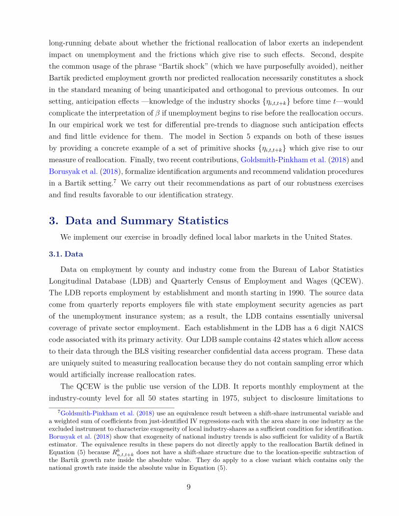
Reallocation timing. If labor market frictions impede reallocation, then the pattern ofnational industry employment growth could lag shifts in ηi,t,t+k and make Bartik growthand reallocation, which depend on realized national industry employment growth rates, poorproxies for the functions of the underlying shocks. To address this potentiality, we measureboth actual and predicted reallocation over two separate, multi-period windows. The firstwindow begins at a national employment peak and lasts through the course of a nationalrecession and subsequent labor market recovery. The second window begins when the labormarket has fully recovered and ends at the start of the next recession. Therefore, we assumethat actual national employment reallocation between the start and end of a recession-recoveryand over an expansion fully reflects the reallocation which would eventually occur as a resultof the idiosyncratic industry shocks, so that the Bartik reallocation instrument embodies thereallocation in an area implied by the national industry shocks.4 This timing also filters outtemporary reallocation induced by differing cyclical sensitivities.

We define a national labor market recession as the period between a private sector em-ployment peak and lasting until the employment trough, a recovery as the period from thetrough until the economy regains its previous peak level, and an expansion as the period be-

4This is the case in our model, as we show in appendix figure 8.

6

Figure 1 – National Business Cycle Partition

70.0

80.0

90.0

100.0

110.0

120.0

130.0

Priv

ate

sect

or e

mpl

oym

ent (

mill

ions

)

Jan80

Jan84

Jan88

Jan92

Jan96

Jan00

Jan04

Jan08

Jan12

Jan16

Recession Recovery Expansion Employment

tween the end of a recovery and the start of the next recession. Thus, we measure reallocationover the 2005-08 expansion using the growth rates of industry employment between June 2005and the private sector employment peak in January 2008 and reallocation during the 2008-14recession-recovery using the growth rates of industry employment between January 2008 andMarch 2014 when employment first regains its January 2008 level. Figure 1 illustrates the labormarket recessions, recoveries, and expansions in our sample. (We treat the 1980-82 period as asingle long recession.) The view of cyclical tightness as the same at the start and end of eachrecession-recovery and expansion cycle echoes the “gaps” view of business cycles advocated byDeLong and Summers (1988). Our main results are not sensitive to this particular partition-ing.5 We apply the same national timing to all local areas to compute predicted and realizedreallocation, allowing for the interpretation of our regressions as pooled cross-sections.6

By construction, national reallocation during a recession-recovery cycle is mean-preservingin overall employment. Measuring reallocation between two periods when total employment

5We use the term “recession” to refer to the period between the private sector employment peak and troughwith the understanding that this definition differs from the periods designated by the NBER. We report ro-bustness to other timing conventions in Section 4.3. We prefer the timing procedure described above for tworeasons. First, when et = et+j , the predicted reallocation measure Rb

a,t,t+j has a natural interpretation asdescribed shortly. Second, we do not see an obvious alternative for how to adjust for demographic trends. Forexample, not only had the national employment-population ratio not recovered its pre-recession level as of theend of 2016, the peak of the series predates the 2000 recession as well. Similarly, the employment-populationratio for prime age males did not regain its previous peak following any downturn since 1975.

6Using local business cycle timing could induce a feedback from local demand/supply shocks to predictedreallocation through the length of the local cycle and thereby reintroduce reverse causality. Because nationaland local cycles are highly correlated, our partitioning captures much of the variation in local business cycles.For example, applying the same recession-recovery/expansion partition to local areas, in our sample a monthlyaverage of 75% of local areas are in a local recession-recovery cycle when the national economy is in a recession-recovery cycle and 68% of local areas are in a local expansion when the national economy is in an expansion.

7

remains unchanged facilitates a natural economic interpretation, since

Ra,t,t+T |ea,t=ea,t+T = 12T

12

I∑i=1

∣∣∣∣∣ea,i,t+T − ea,i,tea,t

∣∣∣∣∣ . (6)

Equation (6) rewrites Ra,t,t+T as the minimum fraction of total period t employment thatchanges industries between t and t+ T , expressed as a monthly flow at an annual rate. Whene−a,t = e−a,t+T , a derivation similar to Equation (6) shows that predicted reallocation Rb

a,t,t+T

has the interpretation of the predicted net quantity of industry employment reshuffling betweent and t+ T as a share of total employment at t, expressed at an annual rate.

Other specification details. An important element of our analysis will be to allow theeffect of reallocation on unemployment to vary by the phase of the business cycle. We arguein Section 5 that the differences in β across business cycle phases are informative about theunderlying economic mechanisms.

Finally, varying the horizon of the unemployment response holding fixed the horizon overwhich reallocation occurs traces out an impulse response function. That is, for months t whichmark the start of a recession or an expansion and letting T denote the length of the recession-recovery or the expansion, we estimate for c ∈ Recession-recovery,Expansion:

∆ua,t,t+j = βj,cRa,t,t+T + gba,t,t+T + Γu′j,cXa,t + εa,t,t+j. (7)

2.3. Discussion

The Bartik research design has the advantage of not requiring the researcher to take a standon the deep industry-level determinants of reallocation in any given period (the ηi in our nota-tion), such as changes in technology, consumer tastes, exchange rates, or trade policy. Rather,the evolution of employment nationally summarizes the consequences of the combination ofthese deep determinants for reallocation. The Bartik approach simply requires that the deepdeterminants produce a common component of industry employment growth across areas, andthat, after residualizing with respect to predicted area growth, these determinants affect localareas only through their effect on reallocation. Not needing to link reallocation to a primitiveshock makes this approach well-suited to the study of business cycle frequency outcomes whichspan multiple cycles, each with its own unique deep determinants of reallocation.

This aspect of the research design also introduces two important limitations. First, westudy the consequences of reallocation but do not attempt to identify its primitive causesand therefore cannot answer how a policy maker might manipulate reallocation if desired.Related, the representation (2) and (3) may not uniquely characterize the system, as ultimatelyunemployment depends on the underlying shocks. Nonetheless, our results shed light on a

8

long-running debate about whether the frictional reallocation of labor exerts an independentimpact on unemployment and the frictions which give rise to such effects. Second, despitethe common usage of the phrase “Bartik shock” (which we have purposefully avoided), neitherBartik predicted employment growth nor predicted reallocation necessarily constitutes a shockin the standard meaning of being unanticipated and orthogonal to previous outcomes. In oursetting, anticipation effects —knowledge of the industry shocks ηi,t,t+k before time t—wouldcomplicate the interpretation of β if unemployment begins to rise before the reallocation occurs.In our empirical work we test for differential pre-trends to diagnose such anticipation effectsand find little evidence for them. The model in Section 5 expands on both of these issuesby providing a concrete example of a set of primitive shocks ηi,t,t+k which give rise to ourmeasure of reallocation. Finally, two recent contributions, Goldsmith-Pinkham et al. (2018) andBorusyak et al. (2018), formalize identification arguments and recommend validation proceduresin a Bartik setting.7 We carry out their recommendations as part of our robustness exercisesand find results favorable to our identification strategy.

3. Data and Summary StatisticsWe implement our exercise in broadly defined local labor markets in the United States.

3.1. Data

Data on employment by county and industry come from the Bureau of Labor StatisticsLongitudinal Database (LDB) and Quarterly Census of Employment and Wages (QCEW).The LDB reports employment by establishment and month starting in 1990. The source datacome from quarterly reports employers file with state employment security agencies as partof the unemployment insurance system; as a result, the LDB contains essentially universalcoverage of private sector employment. Each establishment in the LDB has a 6 digit NAICScode associated with its primary activity. Our LDB sample contains 42 states which allow accessto their data through the BLS visiting researcher confidential data access program. These dataare uniquely suited to measuring reallocation because they do not contain sampling error whichwould artificially increase reallocation rates.

The QCEW is the public use version of the LDB. It reports monthly employment at theindustry-county level for all 50 states starting in 1975, subject to disclosure limitations to

7Goldsmith-Pinkham et al. (2018) use an equivalence result between a shift-share instrumental variable anda weighted sum of coefficients from just-identified IV regressions each with the area share in one industry as theexcluded instrument to characterize exogeneity of local industry-shares as a sufficient condition for identification.Borusyak et al. (2018) show that exogeneity of national industry trends is also sufficient for validity of a Bartikestimator. The equivalence results in these papers do not directly apply to the reallocation Bartik defined inEquation (5) because Rb

a,t,t+k does not have a shift-share structure due to the location-specific subtraction ofthe Bartik growth rate inside the absolute value. They do apply to a close variant which contains only thenational growth rate inside the absolute value in Equation (5).

9

prevent the release of identifying information regarding single establishments.8 We use theQCEW to extend the sample back to 1979 and to fill in states not in our LDB sample.

Two details of the data collection procedure merit mention as they affect our analysis.First, the Federal Unemployment Compensation Amendments of 1976 expanded the numberof industries and establishments covered by unemployment insurance laws, with the result thatthe QCEW expanded its coverage of employment between 1976 and 1980.9 We exclude dataprior to 1978 because the staggered implementation of the coverage expansion across statesproduces substantial measurement difficulties during that period. In effect, we exclude the1976-1980 expansion from the analysis. Second, in 1990 and 1991 the BLS lowered the thresholdrequirements for multi-establishment employers to report employment by single establishment(Farmer and Searson, 1995). As a result, an unusually high number of establishments changeindustry code during those years. While predicted reallocation between the 1990 peak and 1993last-peak should remain mostly unaffected by the reclassifications as long as the changes roughlynet out at the national level, actual reallocation at the local level has sufficient measurementerror to render it unusable.10 We instead develop a two-sample 2sls estimator where we estimatethe first stage excluding the 1990-93 period as described further below.

We combine the LDB data with NAICS 3 digit employment from the QCEW for countiesin states not in the LDB and with 2 digit SIC data for 1975-2000.11 We seasonally adjust allseries at the industry-county level using the multi-step moving average approach contained inthe Census Bureau’s X-11 algorithm. Relative to other data sets with employment by geographyand industry such as the Census Bureau’s County Business Patterns or Longitudinal BusinessDatabase (LBD), the BLS data have the important advantage for business cycle analysis ofproviding monthly rather than annual frequency. We choose SIC 2/NAICS 3 as our level ofindustry detail because our measure of reallocation does not distinguish between movementacross similar or dissimilar industries. The SIC 2/NAICS 3 level allows for enough industrydetail (roughly 80 industries) to generate variation in reallocation across areas while ensuringthat all such reallocation occurs across broadly defined industries. A finer level of detail would

8Even at the NAICS 2 digit level and with counties already aggregated into metropolitan statistical areas(MSAs), roughly one-fifth of potential cells get suppressed for disclosure reasons; the suppressed share rises to35% for MSA-industry cells at the NAICS 3 digit level.

9See http://www.bls.gov/cew/cewbultncur.htm#Coverage.10We are grateful to Jessica Helfand and David Hiles of the BLS for helping to clarify the issues related to

the 1990 and 1991 reporting change. Separately, the NAICS version of the QCEW also contains a number oftranscription errors prior to 2001 which do not appear in the LDB and which we hand correct.

11The QCEW reports employment by county and SIC 2 digit industry beginning in 1975 and by 3 and 4 digitindustry for 1984-2000. We date the 1980s expansion as beginning in October 1983, making the introductionin 1984 of the SIC 3 and 4 digit industry detail redundant for our analysis. The 1987 revision of the SIC madelarge changes to a handful of industry definitions which if uncorrected would result in spurious reallocation. Weadjust for the classification changes by combining each of SIC 36 and 38, SIC 60 and 61, and SIC 73, 87, and 89into a single composite industry. In our analysis, we always interact period fixed effects with the classification(NAICS or SIC) to account for any level differences in reallocation across the two systems.

10

also diminish our ability to make any use of the public data.We aggregate county-level data into Core Based Statistical Areas (CBSAs) using the 2013

OMB county classifications. The Office of Management and Budget (OMB) defines CBSAsas areas “containing a large population nucleus and adjacent communities that have a highdegree of integration with that nucleus” and distinguishes between Metropolitan (MSA) andMicropolitan (MiSA) areas depending on whether the urban core contains at least 50,000 in-habitants. We further aggregate CBSAs into Combined Statistical Areas (CSAs). CSAs consistof adjacent CBSAs that have “substantial employment interchange” and thus better capturethe local labor market. Not all CBSAs belong to a CSA. For example, the San Diego MSAis not part of a CSA, but the Boston-Cambridge-Newton MSA is one of five MSAs in theBoston-Worcester-Providence CSA.

Our main outcome variable is the local unemployment rate and comes from the Bureau ofLabor Statistics Local Area Unemployment Statistics (LAUS) program. We combine publisheddata starting in 1990 with unpublished data available from the LAUS office for 1976-89. For1990-present, the LAUS provide seasonally-adjusted data for MSAs; we augment these data byseasonally adjusting the county data using the same procedure described above for the 1976-89period and for counties not in an MSA and aggregate up to the MSA or CSA level. While theconstruction of county and MSA unemployment rates involves imputation, any noise is likelyto be classical left hand side error and the unemployment rate offers conceptual advantages byreducing the effect of migration on the analysis.

Our final sample includes all MSAs and CSAs containing at least one MSA, with employmentof at least 50,000 in one month, an agricultural share of employment of less than 20%, and wherewe observe at least 95% of private sector employment at the industry level.12 The final samplecontains 1,314 of the 3,144 counties in the United States and covers 86% of 2013 employment.

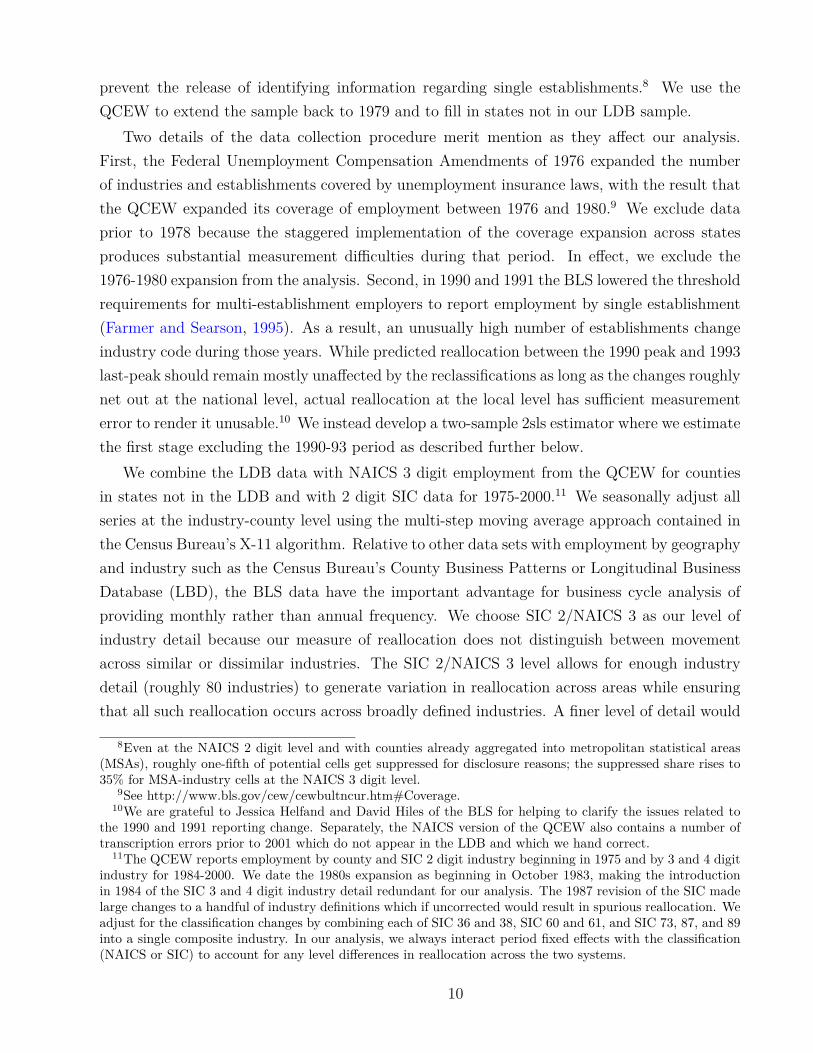
3.2. Trends in National Reallocation

An overview of reallocation at the national level provides useful context for what follows.Table 1 reports national reallocation for each recession-recovery and expansion and at variouslevels of industry aggregation. The shaded rows indicate the recession-recovery episodes. Wemeasure reallocation using SIC definitions for the episodes between 1975 and 2000 and usingNAICS definitions for the episodes beginning after 1990. It helps to group SIC 2 with NAICS3, and SIC 4 with NAICS 6, based on similarity in the number of industries. Reallocationmeasures for the overlapping episodes appear roughly comparable across these definitions.

A number of interesting patterns emerge. First, cross-industry reallocation occurs all the12We exclude areas with a large agricultural share because of the particular difficulty of seasonally adjusting

agricultural employment. The 95% coverage restriction binds because of disclosure limits in CSAs/MSAs locatedat least partly in states not in our LDB sample and for the period 1980-89 when we do not have confidentialdata. As a result, our sample contains fewer CSAs/MSAs in the 1980-89 period than thereafter.

11

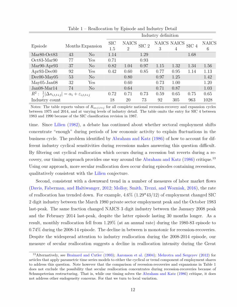
Table 1 – Reallocation by Episode and Industry DetailIndustry definition

Epsiode Months Expansion SIC1.5

NAICS2 SIC 2 NAICS

3NAICS4 SIC 4 NAICS

6Mar80-Oct83 43 No 1.14 1.29 1.68Oct83-Mar90 77 Yes 0.71 0.93Mar90-Apr93 37 No 0.82 1.04 0.97 1.15 1.32 1.34 1.56Apr93-Dec00 92 Yes 0.42 0.60 0.85 0.77 0.95 1.14 1.13Dec00-May05 53 No 0.80 0.97 1.25 1.42May05-Jan08 32 Yes 0.60 0.73 1.00 1.20Jan08-Mar14 74 No 0.64 0.71 0.87 1.03R2 : 1

j|∆si,t,t+j| = αi + εi,t,t+j 0.72 0.71 0.73 0.59 0.65 0.75 0.65

Industry count 18 20 73 92 305 963 1028Notes: The table reports values of Rus,t,t+j for all complete national recession-recovery and expansion cyclesbetween 1975 and 2014, and at varying levels of industry detail. The table omits the entry for SIC 4 between1983 and 1990 because of the SIC classification revision in 1987.

time. Since Lilien (1982), a debate has continued about whether sectoral employment shiftsconcentrate “enough” during periods of low economic activity to explain fluctuations in thebusiness cycle. The problem identified by Abraham and Katz (1986) of how to account for dif-ferent industry cyclical sensitivities during recessions makes answering this question difficult.By filtering out cyclical reallocation which occurs during a recession but reverts during a re-covery, our timing approach provides one way around the Abraham and Katz (1986) critique.13

Using our approach, more secular reallocation does occur during episodes containing recessions,qualitatively consistent with the Lilien conjecture.

Second, consistent with a downward trend in a number of measures of labor market flows(Davis, Faberman, and Haltiwanger, 2012; Molloy, Smith, Trezzi, and Wozniak, 2016), the rateof reallocation has trended down. For example, 4.6% (1.29*43/12) of employment changed SIC2 digit industry between the March 1980 private sector employment peak and the October 1983last-peak. The same fraction changed NAICS 3 digit industry between the January 2008 peakand the February 2014 last-peak, despite the latter episode lasting 30 months longer. As aresult, monthly reallocation fell from 1.29% (at an annual rate) during the 1980-83 episode to0.74% during the 2008-14 episode. The decline in between is monotonic for recession-recoveries.Despite the widespread attention to industry reallocation during the 2008-2014 episode, ourmeasure of secular reallocation suggests a decline in reallocation intensity during the Great

13Alternatively, see Brainard and Cutler (1993); Aaronson et al. (2004); Mehrotra and Sergeyev (2012) forarticles that apply parametric time series models to either the cyclical or trend component of employment sharesto address this question. Note however that the comparison of recession-recoveries and expansions in Table 1does not exclude the possibility that secular reallocation concentrates during recession-recoveries because ofSchumpeterian restructuring. That is, while our timing solves the Abraham and Katz (1986) critique, it doesnot address other endogeneity concerns. For that we turn to local variation.

12

Figure 2 – Map of Predicted Reallocation Per Year, 2008-2014 Cycle

(.73,1.033](.695,.73](.666,.695](.644,.666][.533,.644]

Notes: the figure shows the geographic distribution predicted reallocation per year for the national employmentpeak in January 2008. Due to disclosure limitations, for this figure only we use only data from the public-useQCEW and require a minimum industry employment coverage of 80%.

Recession period (see also Foster, Grim, and Haltiwanger, 2016).14

Third, a large amount of reallocation occurs across broadly-defined industries. For example,of the 6.5% (1.06% per year multiplied by 6.08 years) of employment changing 6 digit NAICSindustry between the January 2008 peak and the March 2014 last-peak, 4.1 p.p. constitutedmovement across 2 digit industries.

Fourth, while individual industries exhibit persistence in their contribution to national real-location, the explanatory power of this relationship lies well below one. We establish this fact byreporting in the penultimate line of the table the R2 from the regression: j−1|∆si,t,t+j| = αi+εi,t.For example, at the NAICS 3 level, the R2 of this regression equals 0.59. Thus, individual indus-try trends leave unexplained 40% of the variation in the contribution of industries to nationalreallocation. This time variation in industry employment trends will in turn contribute tosubstantial variation over time in the predicted reallocation in individual areas.

3.3. Local Reallocation

Figure 2 shows a map of the variation in predicted reallocation during the 2008-2014recession-recovery cycle.15 We split the MSA/CSA observations into quintiles based on theirBartik reallocation and mark higher reallocation levels with darker shades of red. The mapshows that predicted reallocation is not easily explained by geographic factors.

14Interpreted through the lens of our empirical exercises and our model, the decline in reallocation intensityduring the Great Recession translates into a similar increase in unemployment due to reallocation. This isbecause the larger aggregate shock during the Great Recession tightens the downward wage constraint morethan in an average recession. Therefore, a given amount of reallocation generates more unemployment duringthe Great Recession, which compensates for the decline in reallocation intensity.

15For data confidentiality reasons, the map uses only the public-use QCEW data. Greater disclosure limita-tions prior to 2008 make it impossible to report maps at the same level of industry detail for earlier cycles.

13

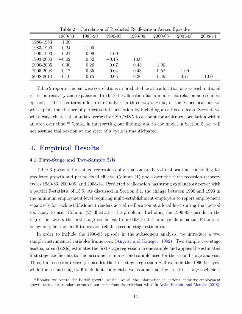
Table 2 – Correlation of Predicted Reallocation Across Episodes1980-83 1983-90 1990-93 1993-00 2000-05 2005-08 2008-14

1980-1983 1.001983-1990 0.24 1.001990-1993 0.21 0.09 1.001993-2000 −0.02 0.52 −0.16 1.002000-2005 0.30 0.26 0.07 0.43 1.002005-2008 0.17 0.35 0.04 0.43 0.52 1.002008-2014 0.10 0.15 0.05 0.26 0.49 0.71 1.00

Table 2 reports the pairwise correlations in predicted local reallocation across each nationalrecession-recovery and expansion. Predicted reallocation has a modest correlation across mostepisodes. These patterns inform our analysis in three ways. First, in some specifications wewill exploit the absence of perfect serial correlation by including area fixed effects. Second, wewill always cluster all standard errors by CSA/MSA to account for arbitrary correlation withinan area over time.16 Third, in interpreting our findings and in the model in Section 5, we willnot assume reallocation at the start of a cycle is unanticipated.

4. Empirical Results4.1. First-Stage and Two-Sample 2sls

Table 3 presents first stage regressions of actual on predicted reallocation, controlling forpredicted growth and period fixed effects. Column (1) pools over the three recession-recoverycycles 1980-83, 2000-05, and 2008-14. Predicted reallocation has strong explanatory power witha partial F-statistic of 15.5. As discussed in Section 3.1, the change between 1990 and 1993 inthe minimum employment level requiring multi-establishment employers to report employmentseparately for each establishment renders actual reallocation at a local level during that periodtoo noisy to use. Column (2) illustrates the problem. Including the 1990-93 episode in theregression lowers the first stage coefficient from 0.98 to 0.21 and yields a partial F-statisticbelow one, far too small to provide reliable second stage estimates.

In order to include the 1990-93 episode in the subsequent analysis, we introduce a twosample instrumental variables framework (Angrist and Krueger, 1992). Two sample two-stageleast squares (ts2sls) estimates the first stage regression in one sample and applies the estimatedfirst stage coefficients to the instruments in a second sample used for the second stage analysis.Thus, for recession-recovery episodes the first stage regression will exclude the 1990-93 cyclewhile the second stage will include it. Implicitly, we assume that the true first stage coefficient

16Because we control for Bartik growth, which uses all the information in national industry employmentgrowth rates, our standard errors do not suffer from the criticism raised in Adão, Kolesár, and Morales (2018).

14

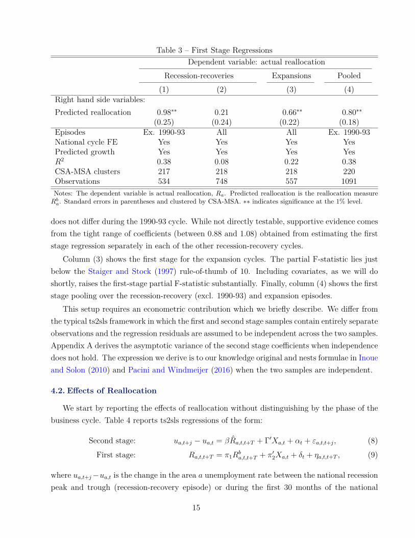
Table 3 – First Stage RegressionsDependent variable: actual reallocation

Recession-recoveries Expansions Pooled(1) (2) (3) (4)

Right hand side variables:Predicted reallocation 0.98∗∗ 0.21 0.66∗∗ 0.80∗∗

(0.25) (0.24) (0.22) (0.18)Episodes Ex. 1990-93 All All Ex. 1990-93National cycle FE Yes Yes Yes YesPredicted growth Yes Yes Yes YesR2 0.38 0.08 0.22 0.38CSA-MSA clusters 217 218 218 220Observations 534 748 557 1091Notes: The dependent variable is actual reallocation, Ra. Predicted reallocation is the reallocation measureRb

a. Standard errors in parentheses and clustered by CSA-MSA. ∗∗ indicates significance at the 1% level.

does not differ during the 1990-93 cycle. While not directly testable, supportive evidence comesfrom the tight range of coefficients (between 0.88 and 1.08) obtained from estimating the firststage regression separately in each of the other recession-recovery cycles.

Column (3) shows the first stage for the expansion cycles. The partial F-statistic lies justbelow the Staiger and Stock (1997) rule-of-thumb of 10. Including covariates, as we will doshortly, raises the first-stage partial F-statistic substantially. Finally, column (4) shows the firststage pooling over the recession-recovery (excl. 1990-93) and expansion episodes.

This setup requires an econometric contribution which we briefly describe. We differ fromthe typical ts2sls framework in which the first and second stage samples contain entirely separateobservations and the regression residuals are assumed to be independent across the two samples.Appendix A derives the asymptotic variance of the second stage coefficients when independencedoes not hold. The expression we derive is to our knowledge original and nests formulae in Inoueand Solon (2010) and Pacini and Windmeijer (2016) when the two samples are independent.

4.2. Effects of Reallocation

We start by reporting the effects of reallocation without distinguishing by the phase of thebusiness cycle. Table 4 reports ts2sls regressions of the form:

Second stage: ua,t+j − ua,t = βRa,t,t+T + Γ′Xa,t + αt + εa,t,t+j, (8)

First stage: Ra,t,t+T = π1Rba,t,t+T + π′2Xa,t + δt + ηa,t,t+T , (9)

where ua,t+j−ua,t is the change in the area a unemployment rate between the national recessionpeak and trough (recession-recovery episode) or during the first 30 months of the national

15

Table 4 – Homogenous Effects over CycleDep. var.: change in unemployment rate

(1) (2) (3)Right hand side variables:Reallocation 0.44+ 0.39∗ 0.60∗∗

(0.25) (0.15) (0.18)National cycle FE Yes Yes YesPredicted growth Yes Yes YesFirst stage coefficient 0.80 1.18 1.11First stage F stat. 18.8 67.7 29.5CSA-MSA clusters 220 220 220First stage observations 1,091 1,091 1,091Second stage observations 1,305 1,305 1,305Notes: The table reports ts2sls regressions. The dependent variable is the change in the unemployment ratebetween the national recession peak and trough (recession-recovery episode) or during the first 30 months ofthe national expansion. Additional controls in column (2) are: lags of employment growth, population growth,and house price growth, each measured from 5 years to 1 year prior to the cycle start; area size, measured bythe log of sample mean employment; and the Herfindahl of industry concentration at the cycle start. Standarderrors in parentheses and clustered by CSA-MSA. +, ∗, ∗∗ indicate significance at the 10%, 5%, and 1% levels.

expansion and Ra,t,t+T = π1Rba,t,t+T + π′2Xa,t + δt is the cross-sample fitted value of reallocation

obtained by applying the first stage regression coefficients to the variables in the second stagesample. The 30 month horizon corresponds to the mean peak-to-trough length in our sample.The endogenous variable Ra,t,t+T and excluded instrument Rb

a,t,t+T measure the monthly flowof reallocation and predicted reallocation, respectively, between the beginning and end of thenational recession-recovery or expansion. Both our simulated model in Section 5 and theempirical impulse response function point to the national trough as the point at which theeffect of reallocation reaches its maximum impact during a recession-recovery, so we start ouranalysis at this horizon. We will shortly report the impulse response function for recession-recoveries.

Table 4 shows that on average over the business cycle reallocation results in higher unem-ployment. Column (1) is our most parsimonious specification and includes inXa,t only predictedgrowth variables measured over the same horizon as reallocation and over the same horizon asthe dependent variable. In anticipation of our next result showing how the effects of reallocationvary by phase of the business cycle, we interact each covariate with an indicator for nationalrecession-recovery or expansion, so that any difference between the effects of reallocation in thistable and the next comes only from allowing the effect of reallocation to vary. The coefficientof 0.44 means that a marginal 1 p.p. of reallocation per year over the course of a cycle causesunemployment to rise by 0.44× 2.5 = 1.1 p.p. during the first 30 months of the cycle. Column(2) adds the following control variables, described in detail in Appendix C: lags of employment

16

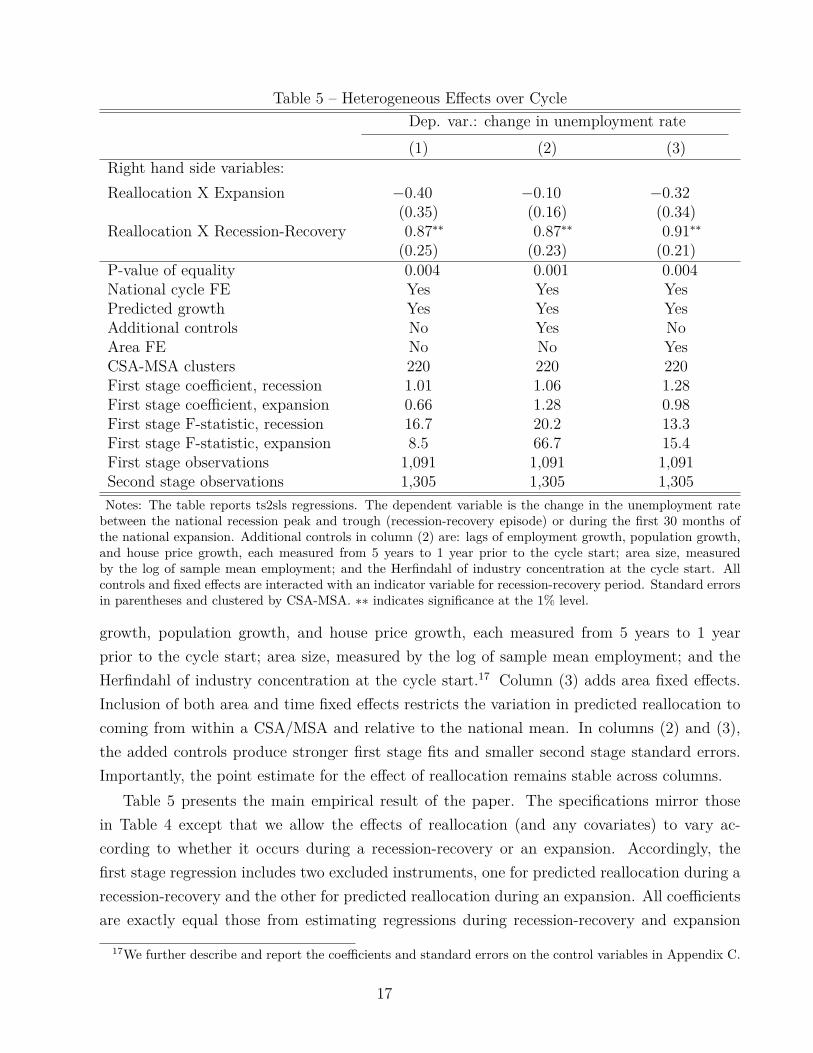
Table 5 – Heterogeneous Effects over CycleDep. var.: change in unemployment rate(1) (2) (3)

Right hand side variables:Reallocation X Expansion −0.40 −0.10 −0.32

(0.35) (0.16) (0.34)Reallocation X Recession-Recovery 0.87∗∗ 0.87∗∗ 0.91∗∗

(0.25) (0.23) (0.21)P-value of equality 0.004 0.001 0.004National cycle FE Yes Yes YesPredicted growth Yes Yes YesAdditional controls No Yes NoArea FE No No YesCSA-MSA clusters 220 220 220First stage coefficient, recession 1.01 1.06 1.28First stage coefficient, expansion 0.66 1.28 0.98First stage F-statistic, recession 16.7 20.2 13.3First stage F-statistic, expansion 8.5 66.7 15.4First stage observations 1,091 1,091 1,091Second stage observations 1,305 1,305 1,305Notes: The table reports ts2sls regressions. The dependent variable is the change in the unemployment ratebetween the national recession peak and trough (recession-recovery episode) or during the first 30 months ofthe national expansion. Additional controls in column (2) are: lags of employment growth, population growth,and house price growth, each measured from 5 years to 1 year prior to the cycle start; area size, measuredby the log of sample mean employment; and the Herfindahl of industry concentration at the cycle start. Allcontrols and fixed effects are interacted with an indicator variable for recession-recovery period. Standard errorsin parentheses and clustered by CSA-MSA. ∗∗ indicates significance at the 1% level.

growth, population growth, and house price growth, each measured from 5 years to 1 yearprior to the cycle start; area size, measured by the log of sample mean employment; and theHerfindahl of industry concentration at the cycle start.17 Column (3) adds area fixed effects.Inclusion of both area and time fixed effects restricts the variation in predicted reallocation tocoming from within a CSA/MSA and relative to the national mean. In columns (2) and (3),the added controls produce stronger first stage fits and smaller second stage standard errors.Importantly, the point estimate for the effect of reallocation remains stable across columns.

Table 5 presents the main empirical result of the paper. The specifications mirror thosein Table 4 except that we allow the effects of reallocation (and any covariates) to vary ac-cording to whether it occurs during a recession-recovery or an expansion. Accordingly, thefirst stage regression includes two excluded instruments, one for predicted reallocation during arecession-recovery and the other for predicted reallocation during an expansion. All coefficientsare exactly equal those from estimating regressions during recession-recovery and expansion

17We further describe and report the coefficients and standard errors on the control variables in Appendix C.

17

Figure 3 – Timing of Effects on Unemployment During Recession-Recovery

-1.0

0.0

1.0

2.0

3.0

4.0

Une

mpl

oym

ent r

ate

chan

ge fr

om p

eak

-20 0 20 40 60 80Months since peak

Notes: The solid line plots the coefficients on reallocation from a regression of the change in the unemploymentrate at different horizons on reallocation. The dashed lines plot the 95% confidence interval for each horizon.

phases separately. Reallocation during a recession-recovery increases unemployment by an eco-nomically large and statistically significant amount. Across columns, the data reject zero effectof reallocation during a recession-recovery at the 1% level, with t-statistics ranging from 3.5 to4.3. In economic magnitude, a one standard deviation increase in predicted reallocation causesan unemployment rate 0.5 p.p. higher (2.5 years×0.87 p.p. per year×0.23 s.d.) by the timenational employment reaches its trough. In contrast, the data do not reject zero effect of real-location on unemployment during expansions, with the point estimates slightly negative. Thedata therefore strongly reject equality of coefficients during a recession-recovery and expansion.

Figure 3 shows the full timing of the effects of reallocation on unemployment during arecession-recovery. The solid line in Figure 3 plots the coefficients βj from a local projection ofthe change in the unemployment rate on reallocation, that is, the coefficients βj from estimatingEquations (8) and (9) allowing j to vary in 6 month increments. The coefficients trace outa hump-shaped impulse response function. Areas undergoing reallocation during a nationalrecession-recovery cycle experience a relative rise in unemployment while national employmentis falling. The effect crests at the national employment trough and reverses as the economyrecovers. The coefficients for one and two years before the national peak indicate little evidenceof areas with large predicted reallocation during the recession-recovery experiencing differentialunemployment rate trends immediately prior to the national peak. The absence of pre-trendsmeans that even if reallocation does not come as a surprise shock at the start of a recession,anticipation effects do not contaminate our estimates of what happens during the recession.

4.3. Robustness

Table 6 groups together a number of sensitivity exercises to assess the robustness of thefinding that reallocation affects unemployment during recessions. Each row of the table reports

18

Table 6 – RobustnessRecession-Recovery

Specification β s.e. P(equality) CSAs Obs.1. Baseline 0.87∗∗ 0.25 0.004 220 13052. Bartik growth vigintiles 0.98∗∗ 0.30 0.404 220 13053. Control for age shares 1.10∗∗ 0.23 0.000 220 13054. Predicted growth by period 0.94∗∗ 0.26 0.008 220 13055. Predicted growth by region 0.99∗∗ 0.30 0.043 220 13056. Drop if area has large industry 0.86∗∗ 0.29 0.002 203 11077. Drop if high manufacturing share 1.25∗∗ 0.45 0.007 193 9608. Drop if high construction share 1.11∗∗ 0.27 0.000 206 9669. Drop if high resources share 1.04∗∗ 0.35 0.160 177 97310. Drop if high health care share 0.70∗ 0.33 0.031 198 98711. Drop persistent industries 1.47∗∗ 0.37 0.004 220 130512. Drop 1990-93 0.86∗∗ 0.31 0.008 220 109113. Drop 2008-14 1.10∗∗ 0.32 0.002 220 110114. HP filter dating 0.88∗∗ 0.28 0.040 220 129115. NAIRU dating 1.15∗ 0.58 0.399 221 124616. Expand window ± 3 months 0.71∗ 0.28 0.067 218 112517. Peak-to-peak reallocation 0.82∗ 0.41 0.030 220 1305Notes: Each row of the table reports the coefficient and standard error for recession-recovery periods and thep-value of equality of coefficients in a recession-recovery and an expansion from a separate regression describedin the first column. All rows additionally include the controls from column (1) of Table 5. The first row,labeled “Baseline”, reproduces column (1) of Table 5. Row 2 controls for episode-specific indicator variables forbelonging to each of twenty quantiles of predicted growth. Row 3 controls for the share of the population in5-year age bins at the start of the cycle. Rows 4 and 5 allow the coefficients on predicted growth to vary bycycle and by region, respectively. Row 6 excludes observations where the area contains at least one industrywith employment of 5% or more of the national total in that industry at the cycle start. Rows 7-10 excludeobservations in the cycle’s top quartile of employment share in the industry indicated. Row 11 excludes fromthe construct of predicted reallocation any industry which either expands or contracts nationally in every cyclein our data. Row 12 drops the 1990-93 cycle. Row 13 drops the 2008-14 cycle. In row 14, a recovery ends whenthe cyclical component of an HP filter of national employment (smoothing parameter 129,600) equals zero. Inrow 15, a recovery ends when the national unemployment rate first equals the CBO’s estimate of the NAIRU.In row 16, the recession-recovery window is extended by 3 months on each side. Row 17 constructs predictedreallocation on a peak-to-peak basis. ∗∗, ∗ denote significance at the 1% or 5% level.

for a separate regression the coefficient and standard error for recession-recovery periods andthe p-value of equality of coefficients in a recession-recovery and an expansion. The first row,labeled “Baseline”, reproduces column (1) of Table 5.

Rows 2 to 5 further expand the control variables in the regression. Row 2 adds non-parametric controls for the Bartik predicted growth rate over the cycle by adding episode-specific indicator variables for belonging to each of twenty quantiles of predicted growth. Thisspecification compares the evolution of unemployment across areas with different predictedreallocation but in the same vigintile of predicted growth. Row 3 controls for the share of thepopulation in 5-year age bins at the start of the cycle. Rows 4 and 5 allow the coefficients on

19

predicted growth to vary by cycle and by region, respectively. The effects of reallocation duringrecession-recoveries increase slightly in each of these specifications and with the exception of row2 the difference in coefficients between recession-recoveries and expansions remain significantat the 5% level.18

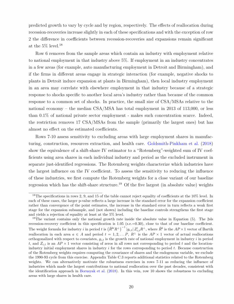
Row 6 removes from the sample areas which contain an industry with employment relativeto national employment in that industry above 5%. If employment in an industry concentratesin a few areas (for example, auto manufacturing employment in Detroit and Birmingham), andif the firms in different areas engage in strategic interaction (for example, negative shocks toplants in Detroit induce expansion at plants in Birmingham), then local industry employmentin an area may correlate with elsewhere employment in that industry because of a strategicresponse to shocks specific to another local area’s industry rather than because of the commonresponse to a common set of shocks. In practice, the small size of CSA/MSAs relative to thenational economy – the median CSA/MSA has total employment in 2013 of 113,000, or lessthan 0.1% of national private sector employment - makes such concentration scarce. Indeed,the restriction removes 17 CSA/MSAs from the sample (primarily the largest ones) but hasalmost no effect on the estimated coefficients.

Rows 7-10 assess sensitivity to excluding areas with large employment shares in manufac-turing, construction, resources extraction, and health care. Goldsmith-Pinkham et al. (2018)show the equivalence of a shift-share IV estimator to a “Rotemberg”-weighted sum of IV coef-ficients using area shares in each individual industry and period as the excluded instrument inseparate just-identified regressions. The Rotemberg weights characterize which industries havethe largest influence on the IV coefficient. To assess the sensitivity to reducing the influenceof these industries, we first compute the Rotemberg weights for a close variant of our baselineregression which has the shift-share structure.19 Of the five largest (in absolute value) weights

18The specifications in rows 2, 9, and 15 of the table cannot reject equality of coefficients at the 10% level. Ineach of these cases, the larger p-value reflects a large increase in the standard error for the expansion coefficientrather than convergence of the point estimates, the increase in the standard error in turn reflects a weak firststage for the expansion subsample, and (not shown) including the baseline controls strengthens the first stageand yields a rejection of equality at least at the 5% level.

19The variant contains only the national growth rate inside the absolute value in Equation (5). The 2slsrecession-recovery coefficient in this specification is 1.05 (s.e.=0.30), close to that of our baseline coefficient.The weight formula for industry i in period t is

(Rb′R⊥

)−1 |gi,t|Z ′i,tR⊥, where Rb is the AP ×1 vector of Bartikreallocation in each area a ∈ A and period t = 1, 2, . . . P , R⊥ is the AP × 1 vector of actual reallocationsorthogonalized with respect to covariates, gi,t is the growth rate of national employment in industry i in periodt, and Zi,t is an AP × 1 vector consisting of zeros in all rows not corresponding to period t and the location-industry initial employment shares in industry i for the rows corresponding to period t. Because constructionof the Rotemberg weights requires computing the covariance of shares and the endogenous variable, we excludethe 1990-93 cycle from this exercise. Appendix Table C.3 reports additional statistics related to the Rotembergweights. We can alternatively motivate the robustness exercises in rows 7-11 as reducing the influence ofindustries which made the largest contributions to national reallocation over the past decades, consistent withthe identification approach in Borusyak et al. (2018). In this vein, row 10 shows the robustness to excludingareas with large shares in health care.

20

for a recession-recovery period, two correspond to manufacturing industries, two to naturalresources extraction, and one to construction. We then remove from the sample areas in thetop quartile of beginning-of-cycle employment share in each of these sectors. Excluding theseareas reduces substantially the Rotemberg weight associated with the particular industry andaddresses directly the concern raised by Goldsmith-Pinkham et al. (2018) of high Rotembergweight industries concentrating in areas which experience other shocks. The coefficients fromthese restricted samples remain close to the baseline.

Row 11 follows Notowidigdo (2011) and keeps all areas but removes from the construction ofpredicted reallocation any industry which either increases or decreases national employment ineach cycle in our data.20 Thus, the variation in row 11 comes only from industries experiencingpersistent but not permanent expansions or contractions. Row 12 excludes the 1990-93 cyclefrom the second sample and reports the coefficient from a conventional 2sls regression. Row 13shows that excluding the Great Recession has a small effect on the results.

Rows 14 to 17 explore robustness to the precise timing definition. Row 14 defines the end ofthe recovery as the first month following a peak in which the cyclical component of an HP filter(smoothing parameter 129,600) of national private sector employment turns positive. In row 15,we define the end of the recovery as the first month in which the national unemployment ratefalls to or below the Congressional Budget Office estimate of the NAIRU. Row 16 expands therecession-recovery window symmetrically by 3 months on each side. Finally, row 17 redefinesthe reallocation timing to measure reallocation between two national employment peaks.21 Thebasic pattern of a statistically significant positive coefficient during recession-recoveries and asmaller coefficient during expansions remains robust to these alterations.

5. Quantitative ModelThe previous section demonstrated that reallocation causes an increase in unemployment if

it occurs during a national recession-recovery, but not if it occurs during an expansion. The risein the unemployment rate concentrates during the recession part of the cycle, with maximumimpact around the national employment trough. We now study a model economy to betterunderstand these patterns. The model illustrates what types of primitive shocks could give riseto our empirical setup and how frictions to labor mobility and downward wage rigidity allowthe model to match the empirical patterns in the data.

20More specifically, we exclude a NAICS (SIC) industry if national employment expands or contracts duringeach cycle in which NAICS (SIC) employment is reported. This procedure identifies 47 of the 165 SIC 2 orNAICS 3 digit industries in our data: 113, 114, 313-316, 322, 323, 325 (NAICS, shrinking); 112, 485, 488, 493,541, 562, 611, 621-624, 712, 722 (NAICS, expanding); 09, 11, 12, 21-23, 31, 66 (SIC, shrinking); 02, 07, 08,47, 58, 62, 64, 67, 72, 73, 75, 79-84 (SIC, expanding). These industries overlap substantially with the set ofindustries with high Rotemberg weights, with five of the ten largest (in absolute value) Rotemberg weights inpersistently shrinking or expanding industries.

21For the 2008-14 cycle, we measure reallocation between the peak in January 2008 and December 2016.

21

5.1. Setup

Time is discrete. The economy consists of A islands, each of which has I industries. Weassume no aggregate uncertainty and perfect consumption insurance within (but not across)islands, which implies an island-specific discount factor ma,t,t+1.

5.1.1. Labor market The labor market in each area-industry operates according to search andmatching principles. At the beginning of period t, industry i in area a contains (1− δt−1)ea,i,t−1

workers employed in the previous period and still attached to their firm, xa,i,t workers searchingfor a job, and va,i,t job vacancies. Hiring occurs at the beginning of the period, with na,i,t

new matches formed. The ea,i,t = (1 − δt−1)ea,i,t−1 + na,i,t workers employed in t engage inproduction. At the end of the period, δtea,i,t of the employed workers exogenously separatefrom their employer. We let ua,i,t = xa,i,t − na,i,t denote the number of unemployed workers inperiod t after the matching process has taken place. Following Christiano et al. (2016), thisconcept of unemployment allows for job-to-job transitions by workers who separate at the end oft−1 but get newly hired at the beginning of t. We let la,i,t = ea,i,t+ua,i,t = (1−δt−1)ea,i,t−1+xa,i,tdenote the total labor force in industry i in area a at time t. We fix the economy-wide laborforce at ∑Aa=1

∑Ii=1 la,i,t = 1.

The firm vacancy posting condition and matching process are standard. Firms post va,i,tvacancies in industry i at cost κ per vacancy. A free entry condition drives the expected valueof a vacancy to zero. The matching function takes the Cobb-Douglas form na,i,t = Mv1−α

a,i,t xαa,i,t.

Letting θa,i,t = va,i,txa,i,t

denote the vacancy-searcher ratio, or industry labor market tightness,searching workers find jobs at rate fa,i,t = Mθ1−α

a,i,t , and firms fill vacancies at rate qa,i,t = Mθ−αa,i,t.Thus, the value of a filled job to the firm, Ja,i,t, and the free entry condition are,

Ja,i,t = (pa,i,t − wa,i,t) + (1− δt)ma,t,t+1Ja,i,t+1, (10)

κ = qa,i,tJa,i,t, (11)

where pa,i,t is the real marginal product and wa,i,t is the real wage.Unemployed workers search in one industry and one area at a time. Their choice of where to

search plays an important role. In line with recent literature, we assume semi-directed search(Kline, 2008; Artuç, Chaudhuri, and McLaren, 2010; Kennan and Walker, 2011; Pilossoph,2014; Dvorkin, 2014). Specifically, at the end of period t, employed workers transition intounemployment in their same industry at rate δt − λt. Both unemployed and employed workersreceive an industry reallocation shock Λa,i,t at exogenous rate λt. An industry reallocationshock Λa,i,t consists of an immediate job separation if previously employed, I time-invariantsector-specific taste parameters ψa,jIj=1, and a draw of I idiosyncratic taste shocks εj,tIj=1

from a distribution F (ε). These taste parameters and shocks enter additively into the worker’svalue function for searching in each sector j = 1, . . . , I. The value functions of an employed

22

worker, Wa,i,t, and an unemployed worker, Ua,i,t, are then,

Wa,i,t = wa,i,t +ma,t,t+1 [(1− δt) + (δt − λt) fa,i,t+1]Wa,i,t+1 + (δt − λt) (1− fa,i,t+1)Ua,i,t+1

+ma,t,t+1λa,t

(E max

j(1− fa,j,t+1)Ua,j,t+1 + fa,j,t+1Wa,j,t+1 + ψa,j + εj,t

), (12)

Ua,i,t = z +ma,t,t+1 (1− λt) [fa,i,t+1Wa,i,t+1 + (1− fa,i,t+1)Ua,i,t+1]

+ma,t,t+1λa,t

(E max

j(1− fa,j,t+1)Ua,j,t+1 + fa,j,t+1Wa,j,t+1 + ψa,j + εj,t

), (13)

where z is the worker’s flow opportunity cost of employment and E the expectations operator.The parameter λ determines the share of unemployed re-optimizing their industry search

market. Equivalently, λ has the interpretation of a stochastic death or retirement shock, witha new generation of workers of mass λ born each period and choosing afresh their industry ofsearch. Holding the share re-optimizing below unity provides one important friction allowingreallocation shocks to affect employment. The ψa,j parameters can be interpreted as permanentpreferences to work in particular sectors. The εj shocks have the interpretation of transitorytaste shocks which make some individuals prefer to work in certain sectors, or of noise shockswhich give individuals private (mis)information about the returns to searching in each sector.Inclusion of these shocks generates two-way gross labor flows across industries. Existence ofgross flows in excess of the net reallocation flows induced by non steady-state dynamics capturesan important feature of reality. Thus, consistent with Pilossoph (2014), net reallocation in ourmodel occurs without requiring changes in the amount of gross flows. The level of λ and thevolatility of the process generating εj together govern the magnitude of gross flows and thedirectness of search across industries.22

We denote the transition probability from industry i to industry j conditional on an in-dustry reallocation shock by πa,ij,t. This probability does not depend on the worker’s previousemployment status or industry, πa,ij,t = πa,kj,t = πa,j,t. We have three laws of motion for theevolution of job seekers, employment, and unemployment:

xa,i,t = δt−1ea,i,t−1 + ua,i,t−1 − λt−1la,i,t−1 + πa,i,t−1λt−1la,t−1,

ea,i,t = (1− δt−1)ea,i,t−1 + fa,i,txa,i,t,

ua,i,t = (1− fa,i,t)xa,i,t.

22The assumption of time dependent, stochastic reallocation shocks Λa,i,t rather than a state-dependent real-location decision and a fixed cost of moving makes the quantity of gross flows exogenous. In an aggregate steadystate, the two approaches are isomorphic. The assumption of time dependent shocks is more computationallytractable for a large number of industries. Quantitatively, the volatility of the preference shocks matters morefor our results than the level of gross flows. Further, since we study the response to very long-lasting industrydispersion shocks, we do not think that allowing for “rest” unemployment as in Alvarez and Shimer (2011) wouldmeaningfully affect the model’s conclusions. We also abstract from geographical mobility. In appendix D.10,we extend the model to incorporate area reallocation. This extension yields quantitatively larger employmentresponses, due to the migration channel, but very similar effects of reallocation on local area unemployment.

23

Wages follow a Nash bargain between the firm and worker, subject to exogenously imposeddownward nominal wage rigidity. This rigidity takes the form

wa,i,t = maxw∗a,i,t, (1− χw)wa,i,t−1/Πa,t, (14)

where w∗a,i,t is the Nash bargained real wage, Πa,t is gross producer price inflation, and χw

is a parameter specifying the maximum permitted decline in the nominal wage. FollowingHall (2005) and Chodorow-Reich and Karabarbounis (2016), exogenous wage rigidity allowsthe model to generate realistic unemployment fluctuations without violating bilateral efficiencyconditions or requiring counterfactual assumptions on the sources of wage rigidity. A largeliterature reports evidence of downward nominal wage rigidity in the data (Kahn, 1997; Cardand Hyslop, 1997; Goette, Sunde, and Bauer, 2007; Dickens, Goette, Groshen, Holden, Messina,Schweitzer, Turunen, and Ward, 2007; Daly and Hobijn, 2014).23

5.1.2. General equilibrium Output of industry i in area a is

Qa,i,t = ηi,tea,i,t, (15)

where ηi,t is (strictly exogenous) labor productivity in industry i which does not vary across is-lands. Industry output is sold under perfect competition at real price PQ

a,i,t to a wholesaler. Thewholesaler combines local industry output into an area-specific good Qa,t using the technology

Qa,t =[ I∑

i

τ1ζ

a,i,tQζ−1ζ

a,i,t

] ζζ−1

, (16)

giving rise to a downward sloping industry-level demand curve Qa,i,t = τa,i,t

(PQa,i,t

PQa,t

)−ζQa,t, and

where ζ ≥ 1 and PQa,t =

[∑Ii τa,i,t(P

Qa,i,t)1−ζ

] 11−ζ . In our calibration, we vary the parameters

τa,i,t across islands to generate variation in steady state employment shares.The real marginal revenue product pa,i,t arising in Equation (10) is the product of industry

productivity and the real price of industry i’s good:

pa,i,t = ηi,tPQa,i,t. (17)

With downward sloping demand, the decline in output engendered by a decline in ηi,t inducesa rise in the real price PQ

a,i,t, such that following a negative productivity shock the marginalrevenue product pa,i,t changes little but output and employment in sector i fall.

23Still, this assumption is not without controversy. Pissarides (2009) shows in the context of a search modelwith exogenous separations that what matters for unemployment fluctuations is the wage rigidity of new hires.Daly and Hobijn (2014) and Gertler, Huckfeldt, and Trigari (2015) provide evidence of rigidity on this margin,including of downward wage rigidity.

24

Closing the model requires specifying the determination of the set of real industry pricesPQa,i,t, overall inflation, and the discount factor ma,t,t+1. We assume that product prices are

determined competitively. An Euler equation for each household determines consumption andthe discount factor. While agents enjoy perfect consumption insurance within an area, assetmarkets across areas allow only for trade of a nominal bond. A central bank follows a standardinterest rate rule that satisfies the Taylor principle. Finally, we allow for a wedge µt betweenthe policy interest rate and the interest rate faced by households, and use an increase in thewedge to generate a demand-induced recession. We provide a detailed discussion and formalstatement of the equations of the remainder of the model in appendix D.

5.2. Calibration

We calibrate a version of the model with two areas and ten industries, A = 2 and I = 10,at monthly frequency. The two areas allow for one small (infinitesimal) area which we treat asrepresentative of a single local CSA/MSA, and one large area representative of the rest of theeconomy. Our choice of ten industries represents a balance between computational feasibilityand ensuring that national industry trends are representative of local industry trends.24

We briefly describe the calibration of the labor market block of the model, shown in Table 7.The parameters are the same in the small and the large area. Appendix D contains furtherdetails and our procedure for finding the model steady state. We obtain a target for the steadystate job finding rate f appropriate to a two state labor market model of 0.5 by updatingthe procedure described in Shimer (2012), and for the job filling rate q of 0.75 from Davis,Faberman, and Haltiwanger (2013). Using the longitudinally linked monthly CPS files, wefind a monthly job separation rate of 0.066. This separation rate exceeds that implied by theprocedure in Shimer (2012) because it includes job-to-job transitions and therefore is moreappropriate for our labor market setting. We also use the longitudinally linked monthly CPSfiles to calculate that 60% of “EUE” spells end with the worker employed in a different 3 digitNAICS industry. This fraction together with the job finding and separation rates determines thereallocation intensity λ. Given that our model has neither aggregate productivity growth nortrend inflation, we set the downward wage rigidity parameter χw to the 0.35% average monthlyincrease in nominal hourly earnings of production and non-supervisory employees. This valueallows nominal wages to fall by 0.35% each month relative to trend, corresponding to zeronominal wage growth. We parameterize the idiosyncratic shocks F (ε) as Type I EV(−ργ, ρ),where γ is Euler’s constant. The parameter ρ governs the directness of search and does not havean easily observed counterpart—it determines the ratio of net reallocation to gross reallocationgiven an increase in dispersion of industry labor demand—and the existing literature provides

24Recall our first-stage coefficient of roughly 1 in Table 3. With I = 2 and one location having a near-100%employment share in the expanding sector, clearly the employment share could not grow at the same rate locallyas it does nationally. We found that I ≥ 10 largely eliminates such cases.

25

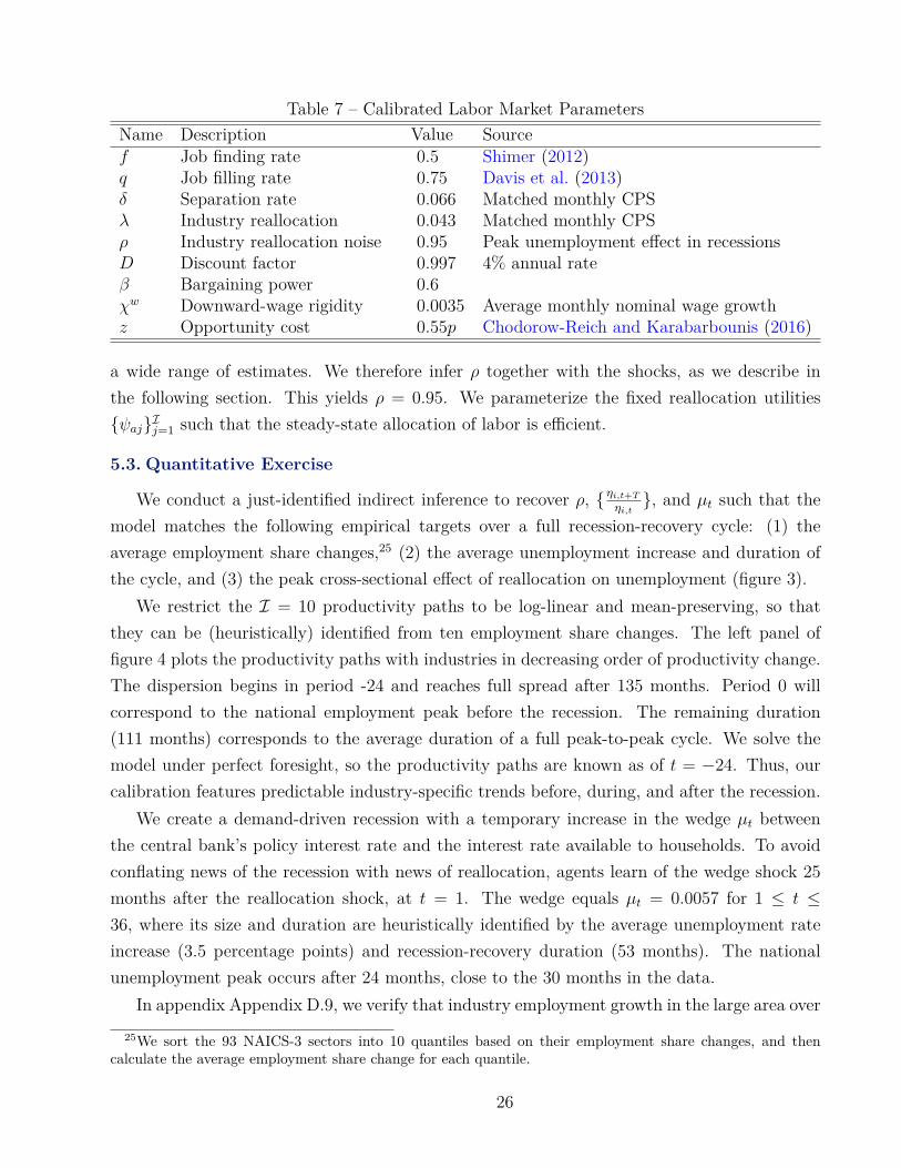
Table 7 – Calibrated Labor Market ParametersName Description Value Sourcef Job finding rate 0.5 Shimer (2012)q Job filling rate 0.75 Davis et al. (2013)δ Separation rate 0.066 Matched monthly CPSλ Industry reallocation 0.043 Matched monthly CPSρ Industry reallocation noise 0.95 Peak unemployment effect in recessionsD Discount factor 0.997 4% annual rateβ Bargaining power 0.6χw Downward-wage rigidity 0.0035 Average monthly nominal wage growthz Opportunity cost 0.55p Chodorow-Reich and Karabarbounis (2016)

a wide range of estimates. We therefore infer ρ together with the shocks, as we describe inthe following section. This yields ρ = 0.95. We parameterize the fixed reallocation utilitiesψajIj=1 such that the steady-state allocation of labor is efficient.

5.3. Quantitative Exercise

We conduct a just-identified indirect inference to recover ρ, ηi,t+Tηi,t, and µt such that the

model matches the following empirical targets over a full recession-recovery cycle: (1) theaverage employment share changes,25 (2) the average unemployment increase and duration ofthe cycle, and (3) the peak cross-sectional effect of reallocation on unemployment (figure 3).

We restrict the I = 10 productivity paths to be log-linear and mean-preserving, so thatthey can be (heuristically) identified from ten employment share changes. The left panel offigure 4 plots the productivity paths with industries in decreasing order of productivity change.The dispersion begins in period -24 and reaches full spread after 135 months. Period 0 willcorrespond to the national employment peak before the recession. The remaining duration(111 months) corresponds to the average duration of a full peak-to-peak cycle. We solve themodel under perfect foresight, so the productivity paths are known as of t = −24. Thus, ourcalibration features predictable industry-specific trends before, during, and after the recession.

We create a demand-driven recession with a temporary increase in the wedge µt betweenthe central bank’s policy interest rate and the interest rate available to households. To avoidconflating news of the recession with news of reallocation, agents learn of the wedge shock 25months after the reallocation shock, at t = 1. The wedge equals µt = 0.0057 for 1 ≤ t ≤36, where its size and duration are heuristically identified by the average unemployment rateincrease (3.5 percentage points) and recession-recovery duration (53 months). The nationalunemployment peak occurs after 24 months, close to the 30 months in the data.

In appendix Appendix D.9, we verify that industry employment growth in the large area over25We sort the 93 NAICS-3 sectors into 10 quantiles based on their employment share changes, and then

calculate the average employment share change for each quantile.

26

Figure 4 – Productivity Paths and Local Predicted Growth and Reallocation

-20 0 20 40 60

Month

0.06

0.07

0.08

0.09

0.1

0.11

0.12Panel A: Industry productivity paths

-1.5 -1 -0.5 0 0.5 1

Predicted Growth (% annualized)

0.7

0.8

0.9

1

1.1

1.2

Pre

dic

ted R

eallo

cation (

% a

nnualiz

ed)

Panel B: Predicted Reallocation and Predicted Growth

Industry 1

Industry 2

Industry 3

Industry 4

Industry 5

Industry 6

Industry 7

Industry 8

Industry 9

Industry 10

Notes: Panel A displays the perfect-foresight productivity paths ηi of each of the i = 1, ..., 10 sectors. Theproductivity paths are mean-preserving in logs. Panel B displays the cross-section of predicted growth andpredicted reallocation in our simulated local areas over a recession-recovery cycle.

a full recession-recovery cycle is highly correlated with the idiosyncratic industry shocks. Wealso show that by the end of the recession-recovery the industry employment distribution hasreached the new steady state level implied by the idiosyncratic productivity shocks. Thus, ourtiming assumption ensures that the Bartik instrument reflects the desired amount of reallocationand not temporary frictions to employment or mobility.

We simulate the model 200 times for different initial employment share in the small area.26

We construct the initial employment shares from ten independent draws from a uniform distri-bution, U [0.06, 1], scaled to sum to one. The positive lower bound on the distribution rules outzero sectoral employment shares as well as employment shares above 65%. The right panel offigure 4 plots a cross-section of the implied predicted growth rates and the predicted reallocationrates for each local area.

The above describes the shocks during the recession-recovery scenario. In the expansionscenario we turn off the interest rate wedge shock. We solve the model by reversing the shocksafter 250 periods and working backward from the initial steady state equilibrium.27

The left panel of figure 5 plots the residualized change in local unemployment from t = 1to t = 24 (the national unemployment peak) against the residualized instrumented reallocationfor the local area. Both variables are residualized with respect to predicted growth over the re-spective cycle and a constant, which corresponds to the second stage of our empirical estimates.The figure highlights a strong positive relationship between (residualized) unemployment and(residualized) instrumented reallocation in a recession, whereas there is no economically signif-icant relationship in an expansion.

26Since the small area is infinitesimal, the solution for the large area is identical in each simulation.27Allowing for a longer time before reversal has little effect on our results.

27

Figure 5 – Model Impulse Response Function and Marginal Effect

-0.3 -0.2 -0.1 0 0.1 0.2 0.3

Residualized Instrumented Reallocation (% annualized)

-0.6

-0.4

-0.2

0

0.2

0.4

0.6

Resid

ualiz

ed C

hange in u

nem

plo

ym

ent (p

.p.)

Panel A: Cross-section at National Unemployment Peak

Recession

Expansion

0 20 40 60 80 100

Month

-0.5

0

0.5

1

1.5

2

2.5

3

Marg

inal effect on u

nem

plo

ym

ent

Panel B: IRF of Marginal Unmployment Effects

Recession

Expansion

Notes: Panel A displays the cross-section of the residualized increase in unemployment from period 0 to 24against the residualized instrumented reallocation, separately for the recession-recovery scenario and the ex-pansion scenario. Panel B displays the marginal effects of realized reallocation based on an IV regression atdifferent horizons.

The right panel plots the marginal effect of reallocation on unemployment for the expan-sion and recession-recovery scenarios. These are the IV coefficients from running regressions ofthe change in unemployment on realized reallocation instrumented with predicted reallocation,controlling for predicted growth and a constant. The marginal effects for t = 24 (the nationalunemployment peak) correspond to the best-fit lines through the points in panel A. Thesemarginal effects of reallocation on unemployment have their data-analog in Table 5 and theplot in Figure 3. In the model, as in the data, the marginal effect of reallocation on unem-ployment is significantly larger and more persistent in recession-recoveries than in expansions.The maximum marginal effect during the recession-recovery peaks at 2.73 after 34 months,consistent with the empirical impulse response function in Figure 3. In contrast, the maximummarginal effect during the expansion is small (0.02), falling within the range of point estimatesreported in Table 5 (after multiplying the latter by 2.5). While the model fits the peak effect inrecessions by construction, the model is corroborated by the dynamics of the marginal effectsand the asymmetry of the expansion results.

5.4. Mechanism

The model replicates the finding that reallocation generates a quantitatively large increasein local unemployment if it occurs during a recession but not if it occurs during an expansion.Compression of the wage distribution during recessions forms a key mechanism underlyingthis difference.28 In expansions the wage constraint does not bind, so real wages rise in the

28Our focus on wage rigidity does not mean that we reject other possible mechanisms. Recent work hashighlighted two: the possibility of search inefficiency or job retraining associated with industry switchers (e.g.Jaimovich and Siu, 2014), and changes in the pool of job seekers during recessions (e.g. Ahn and Hamilton,

28

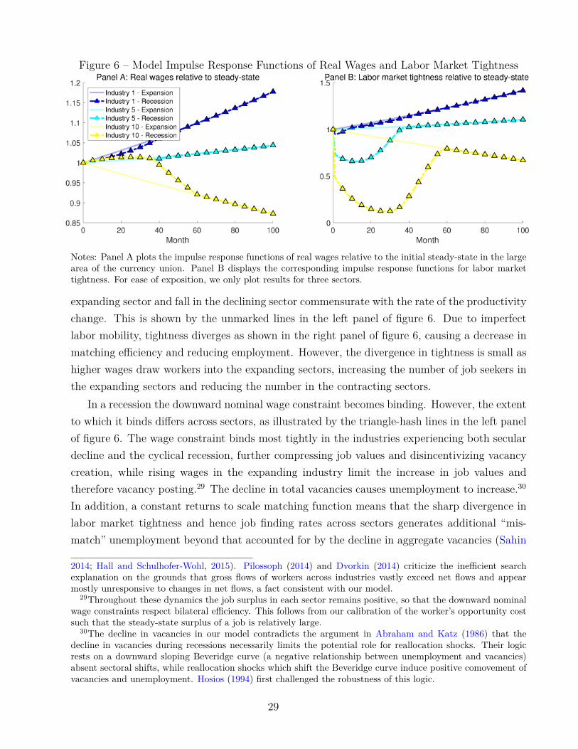
Figure 6 – Model Impulse Response Functions of Real Wages and Labor Market Tightness

Notes: Panel A plots the impulse response functions of real wages relative to the initial steady-state in the largearea of the currency union. Panel B displays the corresponding impulse response functions for labor markettightness. For ease of exposition, we only plot results for three sectors.

expanding sector and fall in the declining sector commensurate with the rate of the productivitychange. This is shown by the unmarked lines in the left panel of figure 6. Due to imperfectlabor mobility, tightness diverges as shown in the right panel of figure 6, causing a decrease inmatching efficiency and reducing employment. However, the divergence in tightness is small ashigher wages draw workers into the expanding sectors, increasing the number of job seekers inthe expanding sectors and reducing the number in the contracting sectors.

In a recession the downward nominal wage constraint becomes binding. However, the extentto which it binds differs across sectors, as illustrated by the triangle-hash lines in the left panelof figure 6. The wage constraint binds most tightly in the industries experiencing both seculardecline and the cyclical recession, further compressing job values and disincentivizing vacancycreation, while rising wages in the expanding industry limit the increase in job values andtherefore vacancy posting.29 The decline in total vacancies causes unemployment to increase.30

In addition, a constant returns to scale matching function means that the sharp divergence inlabor market tightness and hence job finding rates across sectors generates additional “mis-match” unemployment beyond that accounted for by the decline in aggregate vacancies (Sahin

2014; Hall and Schulhofer-Wohl, 2015). Pilossoph (2014) and Dvorkin (2014) criticize the inefficient searchexplanation on the grounds that gross flows of workers across industries vastly exceed net flows and appearmostly unresponsive to changes in net flows, a fact consistent with our model.

29Throughout these dynamics the job surplus in each sector remains positive, so that the downward nominalwage constraints respect bilateral efficiency. This follows from our calibration of the worker’s opportunity costsuch that the steady-state surplus of a job is relatively large.

30The decline in vacancies in our model contradicts the argument in Abraham and Katz (1986) that thedecline in vacancies during recessions necessarily limits the potential role for reallocation shocks. Their logicrests on a downward sloping Beveridge curve (a negative relationship between unemployment and vacancies)absent sectoral shifts, while reallocation shocks which shift the Beveridge curve induce positive comovement ofvacancies and unemployment. Hosios (1994) first challenged the robustness of this logic.

29

Figure 7 – Marginal Effect of Reallocation in Alternative Model Specifications

0 20 40 60 80 100

Month

-0.5

0

0.5

1

1.5

2

2.5

3

Marg

inal effect on u

nem

plo

ym

ent

Panel A: No downward wage rigidity

Recession: Baseline

Expansion: Baseline

Recession: Nash Bargaining

Expansion: Nash Bargaining

0 20 40 60 80 100

Month

-0.5

0

0.5

1

1.5

2

2.5

3

Marg

inal effect on u

nem

plo

ym

ent

Panel B: Panel B: Low reallocation frictions

Recession: Baseline

Expansion: Baseline

Recession: Low Frictions

Expansion: Low Frictions

Notes: Panel A displays the marginal effect of reallocation on unemployment in the baseline model and and whenperiod-by-period Nash bargaining replaces the downward nominal wage rigidity assumption. Panel B contraststhe baseline model with a parameterization that sets the area and industry reallocation noise parameters to 20percent of their baseline values, which weakens reallocation frictions and makes labor search more directed. Ineach case we parameterize the reallocation and recession shocks to hit the same targets as in our baseline.

et al., 2014; Barnichon and Figura, 2015).31

In Table E.1 of the online appendix, we test for the asymmetry of wage compression duringrecessions and expansions using national hourly wages by industry from the CPS and QCEWemployment share changes. Consistent with the model’s mechanism, we find that industrieswith rising employment shares have rising wage differentials during expansions, but that there isno economically or statistically significant relationship between the change in the wage premiumduring a recession and industry share growth.

To illustrate quantitatively the model’s key frictions, panel A of Figure 7 plots the baselinemarginal coefficient impulse response function (the solid blue line) along with counterfactualmarginal coefficients obtained by selectively changing features of the model. The dash-dotlight blue line shows the marginal effects in recession-recoveries with wages determined byNash bargaining in each period. Since this experiment does not feature any nominal rigidity,we induce a recession with a negative productivity shock, calibrated to hit the same recessiontargets as our baseline. Without downward wage rigidity, the effects are much smaller and ofsimilar magnitude across business cycle states.32

31Constant returns to scale makes job finding rates concave in tightness so that minimizing unemploymentholding the number of vacancies fixed requires equalizing job finding rates across sectors. The magnitude ofmismatch unemployment in our model calibrated to features of the Great Recession (employment share changes,depth, duration, and inflation rate) is 1.15 p.p., within the range reported in table 1 of Sahin et al. (2014).

32We kept the baseline ρ in the experiment with Nash Bargaining, since raising ρ to hit the peak marginalunemployment effect resulted in much wider dispersion in the productivity paths, causing negative job surplusin the contracting sector. Appendix Figure 10 displays the comparison with a higher ρ = 4, such that thesurplus remains positive in all sectors. In this case, the marginal effects of reallocation on unemployment underNash Bargaining are too large in expansions, too small in recessions, and counterfactually increase with the

30

Panel B of Figure 7 illustrates the importance of reallocation frictions. The teal and pinkdashed lines report the impulse response functions of the marginal coefficients when the varianceof the reallocation taste shocks εj is reduced to 20% of its baseline values. This change makesthe industry and location choice much more directed. A greater directedness of search per sehas only a minor effect on the employment response to a given set of productivity processes.However, it implies that the same employment share changes across sectors require much lessdispersion in productivity. This limits the dispersion of labor market tightness and the extentto which wage constraints bind asymmetrically across sectors, which results in marginal coeffi-cients of nearly zero in both expansions and recessions. Conversely, appendix figure 11 showsthat an increase in labor market fluidity (Davis and Haltiwanger, 2014) mitigates the adverseemployment consequences of a reallocation shocks.

6. ConclusionReallocation of workers across industries matters asymmetrically over the business cycle.

To establish this fact, we develop a methodology to isolate the secular component of industrydispersion. The methodology identifies reallocation in a local area predicted by the local area’sindustry composition and national trends and orthogonalizes this predicted reallocation withrespect to the direct growth rate consequences of the local industry composition. We apply themethodology to local labor markets over a 35 year period. Areas subjected to more reallocationhave worse local recessions if national employment is depressed, but similar outcomes duringnational expansions.

We interpret the empirical results through the lens of a model of the labor market fea-turing decisions by job-seekers of which industry to search for work. The model delivers thefollowing insights. First, absent labor market frictions or mechanisms which generate stickywages, reallocation does not much affect labor market outcomes. Intuitively, when workers canseamlessly transition across industries, dispersion shocks result in immediate transitions to anew steady state. Second, plausible frictions result in marginal reallocation effects of similarmagnitude to those found in our empirical exercises. Third, compression of wage differentialsduring recessions can explain the asymmetric response of aggregate employment to reallocationduring recession-recoveries and expansions.

Our analysis has implications for policy not explored in this paper. The idiosyncratic indus-try shocks which underlie secular industry reallocation include real shocks such as dispersion inproductivity levels or consumer taste trends. Nonetheless, the ease with which reallocation oc-curs depends sharply on the state of the business cycle. This interaction suggests a possible rolefor monetary policy in accommodating such shocks to “grease the wheels” of reallocation with

horizon.

31

higher inflation. Likewise, the interaction between worker fluidity and industry reallocation inour model suggests a possible role for policy in increasing the fluidity of labor markets to mit-igate against the consequences of industry reallocation shocks. We leave further developmentof these conjectures and other implications to future work.

A. Standard Errors in Two-Sample 2slsThis appendix derives the ts2sls asymptotic standard error when the first and second stage

residuals are not necessarily independent. The notation departs completely from the notationin the main text in order to (roughly) follow Murphy and Topel (1985).

Notation. We assume two possibly interdependent samples of size N1 and N2 drawn fromthe same population where the subscripts 1 and 2 define the samples. We are interested in thefollowing two stage model of the observed data:

Structural equation: Yj = Fjγ +Xjβ + ηj, j = 2, (A.1)

First stage: Fj = WjπW +XjπX + ej, j = 1, (A.2)

Second stage: Yj = Hjπγ +Xjβ + uj, j = 2, (A.3)

where Yj ∼ Nj × 1 denotes a vector of observations of the outcome variable in sample j, Xj ∼Nj ×K is a matrix of included instruments, Fj ∼ Nj ×M is a matrix of endogenous variables,Wj ∼ Nj×L is a matrix of excluded instruments where L ≥M , Hj =

(Xj Wj

)∼ Nj×(K + L)

is the matrix of first stage regressors, ηj ∼ Nj × 1 is the vector of structural residuals, ej ∼Nj×M is the matrix of first stage residuals, uj ∼ Nj×1 is the vector of second stage residuals,β, γ, πX , πW are conforming matrices of parameters, and π =

(πX πW

)′∼ (K + L) × M .

Let π = (H ′1H1)−1H ′1F1 denote the fitted coefficients from the first stage regression and Z2 =(X2 H2π

)∼ N2 × (K +M) denote the matrix of regressors in the second stage.

Assumptions.

E[Z ′jZj

]= Q ∼ (K +M)× (K +M) , (A.4)

E[H ′jHj

]= R ∼ (K + L)× (K + L) , (A.5)

E[Z ′jHj

]= S ∼ (K +M)× (K + L) , (A.6)

E[Z ′juju

′jZj

]= ΩZu ∼ (K +M)× (K +M) , (A.7)

E[H ′jejγγ

′e′jHj

]= ΩH(eγ) ∼ (K + L)× (K + L) , (A.8)

E[Z ′jejγγ

′e′jZj]

= ΩZ(eγ) ∼ (K +M)× (K +M) , (A.9)

E[Z ′jujγ

′ejHj

]= ΩZu(eγ)H ∼ (K +M)× (K +M) , (A.10)

32

E[Z ′jujγ

′ejZj]

= ΩZu(eγ)Z ∼ (K +M)× (K +M) , (A.11)

limN1,N2→∞

N2/N1 = α > 0. (A.12)

Note that in Equations (A.4)–(A.11), the moment conditions hold for any sample, j = 1, 2.

Derivation. Rewriting Equation (A.3) as Y2 = X2β + H2πγ − H2 (π − π) γ + u2, one canderive an expression for the sampling error in the least squares estimator

(β γ

)′:

√N2

β − βγ − γ

=( 1N2

Z ′2Z2

)−1 ( 1√N2

Z ′2u2

)−( 1N2

Z ′2Z2

)−1 1√N2

Z ′2H2 (π − π) γ

=( 1N2

Z ′2Z2

)−1 ( 1√N2

Z ′2u2

)−√N2

N1

( 1N2

Z ′2Z2

)−1 ( 1N2

Z ′2H2

)( 1N1

H ′1H1

)−1 ( 1√N1

H ′1e1

)γ,

where the last line substitutes the first stage relationship√N1 (π − π) =

(1N1H ′1H1

)−1 ( 1√N1H ′1e1

).

Assuming sufficient regularity conditions to invoke a law of large numbers to substituteusing (A.4)–(A.6) and the central limit theorem to use (A.7), (A.8) and (A.10), we have:

√N2

β − βγ − γ

→ N (0,Σ) ,

Σ = Q−1(ΩZu + αSR−1ΩH(eγ)R

−1S ′ −√α(ΩZu(eγ)HR

−1S ′ + SR−1Ω′Zu(eγ)H

))Q−1.

Lemma 1H (H ′H)−1

H ′Z = Z.

Proof: Substitute Z =(X Hπ

), H =

(X W

)and note that Z is in the subspace of H. Thus

the projection of Z onto H yields Z.

Using Lemma 1, SR−1ΩH(eγ)R−1S ′ = ΩZ(eγ), ΩZu(eγ)HR

−1S ′ = ΩZu(eγ)Z , and

Σ = Q−1(ΩZu + αΩZ(eγ) −

√α(ΩZu(eγ)Z + Ω′Zu(eγ)Z

))Q−1. (A.13)

With independent samples and homoskedastic residuals, ΩZu(eγ)Z = 0 and Equation (A.13)reduces to equation (16) in Inoue and Solon (2010).33 When the two samples fully coincide,one can show using u = eγ + η and α = 1 that Σ = Q−1ΩZηQ

−1, the standard expression forthe 2sls variance matrix. A feasible estimator of Σ is:

Σ = (Z ′2Z2)−1 (ΩZ2u2 + αΩZ1(e1γ) −√α(ΩZ1∩2u1∩2(e1∩2γZ1∩2) + Ω′Z1∩2u1∩2(e1∩2γ)Z1∩2

))(Z ′2Z2)−1

,

33Khawand and Lin (2015) show that our ts2sls estimator is equivalent to a weighted average of the 2slsestimator using the overlapping sample and a split-sample 2sls estimator which uses in the second stage onlyobservations not in the first stage sample. Equation (A.13) is more general than their proposition 6 in thatit allows for an arbitrary residual structure. Moreover, their proposition is incorrect because they assumeindependence of the 2sls and ss2sls estimators despite the shared first stage and because of several typos.

33

where the subscript 1 ∩ 2 denotes the intersection of the samples. The functional form of thecross-product matrices ΩZ2u2 ,ΩZ1(e1γ),ΩZ1∩2u1∩2(e1∩2γ)Z1∩2 depends on the assumed covariancestructure of the residuals (homoskedastic, heteroskedastic, clustered, etc.).

ReferencesAaronson, Daniel, Ellen Rissman, and Daniel Sullivan, “Can Sectoral Reallocation Explain theJobless Recovery?,” Federal Reserve Bank of Chicago Economic Perspectives, 2004, (2Q),36–49.

Abraham, Katharine and Lawrence F Katz, “Cyclical Unemployment: Sectoral Shifts or Ag-gregate Disturbances?,” Journal of Political Economy, 1986, 94.

Adão, Rodrigo, Michal Kolesár, and Eduardo Morales, “Shift-Share Designs: Theory and In-ference,” Working Paper 24944, National Bureau of Economic Research August 2018.

Ahn, Hie Joo and James D Hamilton, “Heterogeneity and Unemployment Dynamics,” 2014.Alvarez, Fernando and Robert Shimer, “Search and Rest Unemployment,” Econometrica, 2011,79 (1), 75–122.

Angrist, Joshua and Alan Krueger, “The Effect of Age at School Entry on Educational At-tainment: An Application of Instrumental Variables With Moments From Two Samples,”Journal of the American Statistical Association, 1992, pp. 328–336.

Artuç, Erhan, Shubham Chaudhuri, and John McLaren, “Trade Shocks and Labor Adjustment:A Structural Empirical Approach,” American Economic Review, 2010, 100 (3), 1008–45.

Autor, David H., David Dorn, and Gordon H. Hanson, “The China Syndrome: Local LaborMarket Effects of Import Competition in the United States,” American Economic Review,2013, 103 (6), 2121–68.

Barnichon, Regis and Andrew Figura, “Labor Market Heterogeneity and the Aggregate Match-ing Function,” American Economic Journal: Macroeconomics, October 2015, 7 (4), 222–49.

Bartik, Timothy J., Who Benefits from State and Local Development Policies?, W.E. UpjohnInstitute for Employment Research, 1991.

Berger, David, “Countercyclical Restructuring and Jobless Recoveries,” 2014.Borusyak, Kirill, Peter Hull, and Xavier Jaravel, “Quasi-Experimental Shift-Share ResearchDesigns,” Working Paper 24997, National Bureau of Economic Research September 2018.

Brainard, S. Lael and David M. Cutler, “Sectorial Shifts and Cyclical Unemployment Recon-sidered,” The Quarterly Journal of Economics, 1993, 108 (1), pp. 219–243.

Card, David and Dean Hyslop, “Does Inflation Grease the Wheels of the Labor Market?,” inChristina D. Romer and David H. Romer, eds., Reducing Inflation: Motivation and Strategy,University of Chicago Press, 1997, pp. 71 – 122.

Charles, Kerwin, Erik Hurst, and Matt Notowidigdo, “Masking and Aggregate EmploymentChanges: Housing Booms and Manufacturing Decline During the 2000s,” 2014.

Chodorow-Reich, Gabriel and Loukas Karabarbounis, “The Cyclicality of the Opportunity Costof Employment,” Journal of Political Economy, 2016, 124 (6), 1563–1618.

Christiano, Lawrence, Martin Eichenbaum, and Mathias Trabandt, “Unemployment and Busi-ness Cycles,” Econometrica, 2016, 84 (4), 1523–1569.

Daly, Mary C. and Bart Hobijn, “Downward nominal wage rigidities bend the Phillips curve,”Journal of Money, Credit and Banking, 2014, 46 (S2), 51–93.

Davis, Steven J. and John C. Haltiwanger, “Labor Market Fluidity and Economic Performance,”

34

2014. Jackson Hole Economic Policy Symposium.and John Haltiwanger, “Gross Job Creation, Gross Job Destruction, and Employment Re-allocation,” The Quarterly Journal of Economics, 1992, 107 (3), pp. 819–863., R. Jason Faberman, and John C. Haltiwanger, “The Establishment-Level Behavior of Va-cancies and Hiring,” The Quarterly Journal of Economics, 2013, 128 (2), 581–622., , and John Haltiwanger, “Labor market flows in the cross section and over time,” Journalof Monetary Economics, 2012, 59 (1), 1 – 18. Carnegie-NYU-Rochester Conference Series onPublic Policy at New York University on April 15-16, 2011.

DeLong, J. Bradford, “Identifying Cyclical vs. Structural Unemployment,” Blog post August2010.and Lawrence H. Summers, “How Does Macroeconomic Policy Affect Output?,” BrookingsPapers on Economic Activity, 1988, 1988 (2), pp. 433–494.

Dickens, William T., Lorenz Goette, Erica L. Groshen, Steinar Holden, Julian Messina, Mark E.Schweitzer, Jarkko Turunen, and Melanie E. Ward, “How Wages Change: Micro Evidencefrom the International Wage Flexibility Project,” Journal of Economic Perspectives, June2007, 21 (2), 195–214.

Dvorkin, Maximiliano, “Sectoral Shocks, Reallocation and Unemployment in Competitive La-bor Markets,” 2014. Unpublished manuscript.

Farmer, Tracy and Michael Searson, “Use of Administrative Records in the Bureau of LaborStatistics’ Covered Employment and Wage (ES-202) Program,” Technical Report, Bureau ofthe Census Annual Research Conference 1995.

Foster, Lucia, Cheryl Grim, and John Haltiwanger, “Reallocation in the Great Recession:Cleansing or Not?,” Journal of Labor Economics, 2016, 34 (S1), S293–S331.

Fujita, Shigeru and Giuseppe Moscarini, “Recall Unemployment,” 2013.Garin, Julio, Mike Pries, and Eric Sims, “Reallocation and the Changing Nature of EconomicFluctuations,” 2013.

Gertler, Mark, Chris Huckfeldt, and Antonella Trigari, “Unemployment Fluctuations, MatchQuality, and the Wage Cyclicality of New Hires,” 2015.

Glaeser, Edward L., “Reinventing Boston: 1630�2003,” Journal of Economic Geography,2005, 5 (2), 119–153.

Goette, Lorenz, Uwe Sunde, and Thomas Bauer, “Wage Rigidity: Measurement, Causes andConsequences,” The Economic Journal, 2007, 117 (524), F499–F507.

Goldsmith-Pinkham, Paul, Isaac Sorkin, and Henry Swift, “Bartik Instruments: What, When,Why, and How,” Technical Report, National Bureau of Economic Research 2018.

Groshen, Erica and Simon Potter, “Has structural change contributed to a jobless recovery?,”Current Issues in Economics and Finance, 2003, 9 (8).

Hall, Robert, “Employment Fluctuations with Equilibrium Wage Stickiness,” American Eco-nomic Review, 2005, 95 (1), 50–65.and Sam Schulhofer-Wohl, “Measuring Job-Finding Rates and Matching Efficiency withHeterogeneous Jobseekers,” 2015. NBER Working Paper No. 20939.

Hosios, Arthur J., “Unemployment and Vacancies with Sectoral Shifts,” The American Eco-nomic Review, 1994, 84 (1), 124–144.

Inoue, Atsushi and Gary Solon, “Two-Sample Instrumental Variables Estimators,” The Reviewof Economics and Statistics, 2010, 92 (3), 557–561.

Jackman, Richard and Stephen Roper, “Structural Unemployment,” Oxford Bulletin of Eco-nomics and Statistics, 1987, 49 (1), 9–36.

35

Jaimovich, Nir and Henry Siu, “The Trend is the Cycle: Job Polarization and Jobless Recov-eries,” 2014.

Kahn, Shulamit, “Evidence of Nominal Wage Stickiness from Microdata,” The American Eco-nomic Review, 1997, 87 (5), pp. 993–1008.

Kennan, John and James R. Walker, “The Effect of Expected Income on Individual MigrationDecisions,” Econometrica, 2011, 79 (1), 211–251.

Khawand, Christopher and Wei Lin, “Finite Sample Properties and Empirical Applicability ofTwo-Sample Two-Stage Least Squares,” 2015.

Kline, Patrick, “Understanding Sectoral Labor Market Dynamics: An Equilibrium Analysis ofthe Oil and Gas Field Services Industry,” 2008. Unpublished manuscript.

Koenders, Kathryn and Richard Rogerson, “Organizational dynamics over the business cycle:a view on jobless recoveries,” Review, 2005, (Jul), 555–580.

Krugman, Paul, “Jobs and Skills and Zombies,” Blog post March 2014.Lilien, David M, “Sectoral shifts and cyclical unemployment,” The Journal of Political Econ-omy, 1982, pp. 777–793.

Mehrotra, Neil R and Dmitriy Sergeyev, “Sectoral Shocks, the Beveridge Curve and MonetaryPolicy,” mimeo, 2012.

Molloy, Raven, Christopher L. Smith, Riccardo Trezzi, and Abigail Wozniak, “UnderstandingDeclining Fluidity in the U.S. Labor Market,” Brookings Papers on Economic Activity, 2016,Spring.

Murphy, Kevin and Robert Topel, “The Evolution of Unemployment in the United States:1968-1985,” in Stanley Fischer, ed., NBER Macroeconomics Annual 1987, Vol. 2 The MITPress 1987, pp. 11–68.

Murphy, Kevin M. and Robert H. Topel, “Estimation and Inference in Two-Step EconometricModels,” Journal of Business & Economic Statistics, 1985, 3 (4), 370–379.

Notowidigdo, Matthew J., “The Incidence of Local Labor Demand Shocks,” June 2011.Pacini, David and Frank Windmeijer, “Robust inference for the Two-Sample 2SLS estimator,”Economics Letters, 2016, 146, 50 – 54.

Pilossoph, Laura, “Sectoral Shocks and Move Unemployment,” 2014. Unpublished manuscript.Pissarides, Christopher A., “The Unemployment Volatility Puzzle: Is Wage Stickiness theAnswer?,” Econometrica, 2009, 77 (5), 1339–69.

Sahin, Aysegül, Joseph Song, Giorgio Topa, and Giovanni L. Violante, “Mismatch Unemploy-ment,” American Economic Review, 2014, 104 (11), 3529–64.

Schmitt-Grohé, Stephanie and Martın Uribe, “Downward Nominal Wage Rigidity, CurrencyPegs, and Involuntary Unemployment,” Journal of Political Economy, 2016, 124 (5), 1466–1514.

Schumpeter, Joseph A., Capitalism, Socialism, and Democracy 1942.Shimer, Robert, “Mismatch,” American Economic Review, September 2007, 97 (4), 1074–1101., “Reassessing the Ins and Outs of Unemployment,” Review of Economic Dynamics, 2012,15, 127–48.

Staiger, Douglas and James H. Stock, “Instrumental Variables Regression with Weak Instru-ments,” Econometrica, 1997, 65 (3), 557–586.

Walsh, Carl E, “Labor Market Search, Sticky Prices, and Interest Rate Policies,” Review ofeconomic Dynamics, 2005, 8 (4), 829–849.

36