secular dynamics of an exterior test particle: the inverse...

MNRAS 000, 1–12 (2017) Preprint 7 November 2017 Compiled using MNRAS LATEX style file v3.0

Secular Dynamics of an Exterior Test Particle:

The Inverse Kozai and Other Eccentricity-Inclination Resonances

Benjamin R. Vinson1⋆, Eugene Chiang2,3†1Department of Physics, 366 LeConte Hall, University of California, Berkeley, 94720, USA2Department of Astronomy, 501 Campbell Hall, University of California, Berkeley 94720-3411, USA3Department of Earth and Planetary Science, 307 McCone Hall, University of California, Berkeley 94720, USA

7 November 2017

ABSTRACT

The behavior of an interior test particle in the secular three-body problem has been studiedextensively. A well-known feature is the Lidov-Kozai resonance in which the test particle’sargument of periastron librates about±90 and large oscillations in eccentricity and inclinationare possible. Less explored is the inverse problem: the dynamics of an exterior test particle andan interior perturber. We survey numerically the inverse secular problem at a fixed semimajoraxis ratio of 0.2, expanding the potential to hexadecapolar order and correcting an errorin the published expansion. Four secular resonances are uncovered that persist in full N-body treatments (angles below are referred to the perturber’s orbit plane, with longitude zeropointing toward the perturber’s periapse): (i) an orbit-flipping quadrupole resonance requiringa non-zero perturber eccentricity e1, in which the test particle’s longitude of ascending nodeΩ2 librates about ±90; (ii) a hexadecapolar resonance (the “inverse Kozai resonance”) forperturbers that are circular or nearly so and inclinations I ≃ 63/117, in which the argumentof periastron ω2 librates about 90 and which can vary the particle eccentricity by ∆e2 ≃ 0.2;(iii) an octopole “apse-aligned” resonance at I ≃ 46/107 wherein ω2 + Ω2 librates about0 and ∆e2 grows with e1; and (iv) an octopole resonance at I ≃ 73/134 wherein ω2 − Ω2librates about 0 and∆e2 can be as large as 0.3 for small but non-zero e1. Qualitatively, the moreeccentric the perturber, the more the particle’s eccentricity and inclination vary; also, morepolar orbits are more chaotic. Our solutions to the inverse problem have potential applicationto the Kuiper belt and debris disks, and hierarchical stellar systems.

Key words: celestial mechanics – binaries: general – planets and satellites: dynamical evolu-tion and stability – Kuiper belt: general

1 INTRODUCTION

In the restricted three-body problem, the Lidov-Kozai resonanceprovides a way for an external perturber to torque test particle or-bits to high eccentricity and inclination (Lidov 1962; Kozai 1962).When the perturber’s orbit is circular (e2 = 0), and when theinclination I between the test particle’s orbit and the perturber’sexceeds arccos

√

3/5 ≃ 39, the test particle’s argument of peri-astron ω1 can librate (oscillate) about either 90 or 270: theseare the fixed points of the Lidov-Kozai (“Kozai” for short) reso-nance.1 The larger the libration amplitude (ω1 can even circulate),the greater the eccentricity variations. For circular perturbers, the

⋆ E-mail: [email protected]† E-mail: [email protected] Throughout this paper, the subscript “1” denotes the interior body andsubscript “2” denotes the exterior body; by definition, the orbital semimajoraxes a1 < a2. These subscripts apply regardless of whether the body is atest particle or a perturber.

test particle eccentricity e1 can cycle between 0 and 1 as the incli-nation I cycles between 90 and 39;2 e1 and I seesaw to conserve

J1z ∝√

1 − e21 cos I, the test particle’s vector angular momentum

projected onto the perturber’s orbit normal. For eccentric externalperturbers (e2 , 0), the gravitational potential is no longer ax-isymmetric, and the test particle’s J1z is now free to vary, which itcan do with a vengeance: the test particle can start from a nearlycoplanar, prograde orbit (J1z > 0) and “flip” to being retrograde(J1z < 0; e.g., Lithwick & Naoz 2011). The large eccentricitiesand inclinations accessed by the Kozai mechanism have found ap-plication in numerous settings: enabling Jupiter to send cometsonto sun-grazing trajectories (e.g., Bailey et al. 1992); delineatingregions of orbital stability for planetary satellites perturbed by exte-

2 There is also a retrograde branch for the standard Kozai resonance inwhich I cycles between 90 and 141. In this paper we will encounter severalresonances for which retrograde fixed points are paired with prograde fixedpoints, but will sometimes focus on the prograde branches for simplicity.

© 2017 The Authors

2 Vinson & Chiang

rior satellites and the Sun (e.g., Carruba 2002; Nesvorny et al. 2003;Tremaine & Yavetz 2014); merging compact object binaries in triplesystems (e.g., Kushnir et al. 2013; Silsbee & Tremaine 2017); andexplaining the orbits of eccentric or short-period extrasolar planets(e.g., Wu & Murray 2003), including hot Jupiters with their largespin-orbit obliquities (Naoz et al. 2011).

The Kozai resonance is a secular resonance (i.e., it does not de-pend on orbital longitudes, which are time-averaged away from theequations of motion) that applies to an interior test particle perturbedby an exterior body. Curiously, the “inverse” secular problem—an exterior test particle and an interior perturber—does not seemto have received as much attention as the conventional problem.Gallardo et al. (2012) studied the inverse problem in the context ofKuiper belt objects perturbed by Neptune and the other giant planets,idealizing the latter as occupying circular (e1 = 0) and coplanar or-bits, and expanding the disturbing function (perturbation potential)to hexadecapolar order in α ≡ a1/a2. They discovered an analogousKozai resonance in which ω2 librates about either +90 or −90,when I ≃ arccos

√

1/5 ≃ 63 (see also Tremaine & Yavetz 2014).Eccentricity variations are stronger inside this “inverse Kozai” or“ω2 resonance” than outside. Thomas & Morbidelli (1996) also as-sumed the solar system giant planets to be on circular coplanarorbits, dispensing with a multipole expansion and numerically com-puting secular Hamiltonian level curves for an exterior test particle.For a2 = 45 AU, just outside Neptune’s orbit, resonances appear athigh I and e2 that are centered on ω2 = 0 and 180.

Naoz et al. (2017) also studied the inverse problem, expand-ing the potential to octopolar order and considering non-zero e1.Orbit flipping was found to be possible via a quadrupole-level “Ω2resonance” that exists only when e1 , 0 and for which Ω2 libratesabout either +90 or −90. As e1 increases, the minimum I atwhich orbits can flip decreases. All of this inclination behavior ob-tains at the quadrupole level. Octopole terms were shown to enabletest particles to switch back and forth between one libration center(Ω2 = +90) and another (Ω2 = −90), modulating the inclinationevolution and introducing chaos, particularly at high e1.

In this paper we explore more systematically the inverse prob-lem, expanding the perturbation potential to hexadecapolar orderand considering non-zero e1. In addition to studying more closelythe hexadecapolar inverse Kozai resonance found by Gallardo et al.(2012) and how it alters when e1 increases, we will uncoverstrong, octopolar resonances not identified by Naoz et al. (2017).By comparison with the latter work, we focus more on the testparticle’s eccentricity variations than on its inclination variations.We are interested, for example, in identifying dynamical chan-nels that can connect planetary systems with more distant reser-voirs of minor bodies, e.g., the “extended scattered” or “detached”Kuiper belt (e.g., Sheppard & Trujillo 2016), or the Oort cloud(e.g., Silsbee & Tremaine 2016). Another application is to extra-solar debris disks, some of whose scattered light morphologiesappear sculpted by eccentric perturbers (e.g., Lee & Chiang 2016).We seek to extend such models to large mutual inclinations (e.g.,Pearce & Wyatt 2014; Nesvold et al. 2016; Zanardi et al. 2017).

This paper is organized as follows. In Section 2 we write downthe secular disturbing function of an interior perturber to hexade-capolar order in α = a1/a2. There we also fix certain parameters(masses and semimajor axes; e.g., α = 0.2) for our subsequent nu-merical survey. Results for a circular perturber are given in Section3 and for an eccentric perturber in Section 4, with representativesecular integrations tested against N-body integrations. We wrap upin Section 5.

2 SECULAR DISTURBING FUNCTION FOR EXTERIOR

TEST PARTICLE

The disturbing function of Yokoyama et al. (2003, hereafter Y03)is for the conventional problem: an interior test particle (satelliteof Jupiter) perturbed by an exterior body (the Sun). We may adapttheir R to our inverse problem of an exterior test particle perturbedby an interior body by a suitable reassignment of variables. Thisreassignment is straightforward because the disturbing function isproportional to 1/∆, where ∆ is the absolute magnitude of the dis-tance between the test particle and the perturber (Y03’s equation2, with the indirect term omitted because that term vanishes aftersecular averaging). This distance ∆ is obviously the same betweenthe conventional and inverse problems, and so the Legendre poly-nomial expansion of 1/∆ performed by Y03 for their problem holdsjust as well for ours.

The change of variables begins with a simple replacing ofsubscripts. We replace Y03’s subscript ⊙ (representing the Sun,their exterior perturber) with “2” (our exterior test particle). Fortheir unsubscripted variables (describing their interior test particle),we add a subscript “1” (for our interior perturber). Thus we have:

a → a1 (1)

a⊙ → a2 (2)

e → e1 (3)

e⊙ → e2 , (4)

where a is the semimajor axis and e is the eccentricity. Since we areinterested in the inverse problem of an interior perturber, we replacetheir perturber mass M⊙ with our perturber mass:

M⊙ → m1 . (5)

Their inclination I is the mutual inclination between the interior andexterior orbits; we leave it as is.

Mapping of the remaining angular variables requires morecare. Y03’s equations (6) and (7) take the reference plane to coincidewith the orbit of the exterior body—this is the invariable plane whenthe interior body is a test particle. We want the reference plane tocoincide instead with the orbit of the interior body (the invariableplane for our inverse problem). To convert to the new referenceplane, we use the relation

Ω1 −Ω2 = π (6)

for longitude of ascending node Ω, valid whenever the referenceplane is the invariable plane for arbitrary masses 1 and 2 (the vectorpole of the invariable plane is co-planar with the orbit normals ofbodies 1 and 2, and lies between them). We therefore map Y03’s Ωto

Ω→ Ω1 → Ω2 + π . (7)

and their argument of periastron ω to

ω ≡ ( −Ω) → (1 −Ω1) → (1 − π −Ω2) (8)

where is the longitude of periastron. Although1 remains mean-ingful in our new reference plane, Ω1 and ω1 are no longer mean-ingful, and are swapped out using (7) and (8). Finally

⊙ → 2 . (9)

Armed with (1)–(9), we can now re-write equations (6)–(8) ofY03 to establish the secular disturbing function R for an exteriortest particle perturbed by an interior body of mass m1, expanded to

MNRAS 000, 1–12 (2017)

Exterior Test Particle 3

hexadecapole order:

b1 = −(5/2)e1 − (15/8)e31 (10)

b2 = −(35/8)e31 (11)

c1 = Gm1a21

1

a32(1 − e2

2)3/2(12)

c2 = Gm1a31

e2

a42(1 − e2

2)5/2(13)

c3 = Gm1a41

1

a52(1 − e2

2)7/2(14)

d∗1 = 1 + (15/8)e21 + (45/64)e4

1 (15)

d2 = (21/8)e21(2 + e2

1) (16)

d3 = (63/8)e41 (17)

cI ≡ cos I (18)

sI ≡ sin I (19)

R2 =1

8

(

1 +3

2e21

)

(3cI2 − 1) + 15

16e21sI2 cos 2(1 −Ω2) (20)

R3 =1

64

[(

−3 + 33cI + 15cI2 − 45cI3)

b1 cos(2 +1 − 2Ω2)

+

(

−3 − 33cI + 15cI2+ 45cI3

)

b1 cos(2 −1)

+

(

15 − 15cI − 15cI2+ 15cI3

)

b2 cos(2 + 31 − 4Ω2)

+

(

15 + 15cI − 15cI2 − 15cI3)

b2 cos(2 − 31 + 2Ω2)]

(21)

R4 =3

16

(

2 + 3e22

)

d∗1 − 495

1024e22 − 135

256cI2 − 165

512

+

315

512cI4+

945

1024cI4e2

2 − 405

512cI2e2

2

+

(

105

512cI4+

315

1024e22 − 105

256cI2+

105

512− 315

512cI2e2

2

+

315

1024cI4e2

2

)

d3 cos 4(1 −Ω2)

+

105

512

(

cI3 − cI − 1

2cI4+

1

2

)

d3e22 cos(41 + 22 − 6Ω2)

+

105

512

(

−cI3+ cI − 1

2cI4+

1

2

)

d3e22 cos(41 − 22 − 2Ω2)

+

(

45

64cI2 − 45

512− 315

512cI4

)

e22 cos(22 − 2Ω2)

+

(

15

16cI2+

45

32cI2e2

2 − 45

256e22 − 15

128− 315

256cI4e2

2

−105

128cI4

)

d2 cos(21 − 2Ω2)

+

(

15

256− 45

128cI2+

75

256cI +

105

256cI4

− 105

256cI3

)

d2e22 cos(21 + 22 − 4Ω2)

+

(

15

256− 45

128cI2 − 75

256cI +

105

256cI4

+

105

256cI3

)

d2e22 cos(21 − 22) (22)

R = R2c1 + R3c2 + R4c3 . (23)

A few notes: (i) this disturbing function includes only the quadrupole

(R2c1), octopole (R3c2), and hexadecapole (R4c3) terms; themonopole term has been dropped (it is equivalent to adding m1to the central mass m0), as has the dipole term which orbit-averagesto zero; (ii) there are typos in equation (6) of Y03: their ci’s aremissing factors of M⊙ (→ m1); (iii) we have starred d∗1 in equa-tion (15) to highlight that this term as printed in Y03 is in error,as brought to our attention by Matija Ćuk, who also provided thecorrection. We have verified this correction independently by com-puting the hexadecapole disturbing function in the limit I = 0 ande2 = 0.

We insert the disturbing function R into Lagrange’s planetaryequations for Ûe2, ÛΩ2, Û 2, and ÛI (equations 6.146, 6.148, 6.149,and 6.150 of Murray & Dermott 2000). These coupled ordinarydifferential equations are solved numerically using a Runge-Kutta-Dormand-Prince method with stepsize control and dense output(runge_kutta_dopri5 in C++).

2.1 Fixed Parameters

The number of parameters is daunting, even for the restricted, secu-lar three-body problem considered here. Throughout this paper, wefix the following parameters:

a1 = 20 AU (24)

a2 = 100 AU (25)

m0 = 1M⊙ (26)

m1 = 0.001 m0 . (27)

These choices largely set the timescale of the test particle’s evolution(see Section 3). The ratio of orbital semimajor axes is fixed atα ≡ a1/a2 = 0.2.

With no loss of generality, we align the apsidal line of theperturber’s orbit with the x-axis:

1 = 0 . (28)

The remaining variables of the problem are e1, e2, I, ω2, and Ω2.Often in lieu of e2 we will plot the periastron distance q2 = a2(1−e2)to see how close the test particle comes to the perturber. Once theorbits cross or nearly cross (i.e., once q2 . a1(1 + e1) = 20–35AU), our secular equations break down and the subsequent evolutioncannot be trusted.

To the extent that R is dominated by the first quadrupole termin (20) proportional to (3 cos2 I − 1), more positive R correspondsto more co-planar orbits (i.e., wires 1 and 2 closer together). Thenumerical values for R quoted below have been scaled to avoid largeunwieldy numbers; they should be multiplied by 3.55×106 to bringthem into cgs units.

3 CIRCULAR PERTURBER

When e1 = 0, the octopole contribution to the potential vanishes,but the quadrupole and hexadecapole contributions do not.

Because the potential for a circular perturber is axisymmet-ric, the z-component of the test particle’s angular momentum isconserved (we omit the subscript 2 on Jz for convenience):

Jz ≡√

1 − e22 cos I (29)

where we have dropped the dependence of the angular momentumon a2, since semimajor axes never change in secular dynamics. Wetherefore have two constants of the motion: Jz and the disturbingfunction itself (read: Hamiltonian), R. Smaller Jz corresponds tomore highly inclined and/or more eccentric test particle orbits.

MNRAS 000, 1–12 (2017)

4 Vinson & Chiang

3.1 The Inverse Kozai (ω2) Resonance

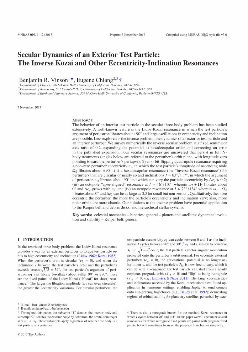
Figure 1 gives a quick survey of the test particle dynamics fore1 = 0. For a restricted range in Jz ≃ 0.42–0.45, the test particle’sargument of periastron ω2 librates about either 90 or 270, withconcomitant oscillations in q2 (equivalently e2) and I. This is theanalogue of the conventional Kozai resonance, exhibited here by anexterior test particle; we refer to it as the “inverse Kozai resonance”or the “ω2 resonance.” The inverse Kozai resonance appears only athexadecapole order; it originates from the term in (22) proportionalto e2

2 cos(22 − 2Ω2) = e22 cos 2ω2.3

The inverse Kozai resonance appears near

I(ω2−res) = arccos(±√

1/5) ≃ 63 and 117 (30)

which, by Lagrange’s planetary equations and (20), are the specialinclinations at which the quadrupole precession rate

dω2

dt

quad,e1=0=

3

8

m1

m0

(

a1

a2

)2n2

(1 − e2)2(

5 cos2 I − 1)

(31)

vanishes, where n2 is the test particle mean motion; see Gal-lardo et al. (2012, their equation 11 and subsequent discussion). AtI = I(ω2−res), fixed points appear atω2 = 90 andω2 = 270. Thecritical angles 63 and 117 are related to their well-known Kozaicounterparts of 39 and 141 (i.e., arccos(±

√

3/5)), but the corre-spondence is not exact. In the conventional problem, the inclinationsat which the fixed points (ω1 = ±90, Ûω1 = 0) appear vary from

case to case; they are given by I = arccos

[

±√

(3/5)(1 − e21)

]

=

arccos[

±(3/5)1/4 |J1z |1/2]

, where J1z ≡√

1 − e21 cos I is con-

served at quadrupole order (e.g., Lithwick & Naoz 2011). But forour inverse problem, the fixed points (ω2 = ±90, Ûω2 = 0) appear atfixed inclinations I of 63 and 117 that are independent of Jz (fore1 = 0). In this sense, the inverse Kozai resonance is “less flexible”than the conventional Kozai resonance.

The ω2 resonance exists only in a narrow range of Jz that isspecific to a given α = a1/a2, as we have determined by numericalexperimentation. Outside this range, ω2 circulates and e2 and I

hardly vary (Figure 1). Fine-tuning Jz can produce large resonantoscillation amplitudes in e2 and I; some of these trajectories leadto orbit crossing with the perturber.

3.1.1 Precession Timescales

To supplement (31), we list here for ease of reference the remainingequations of motion of the test particle, all to leading order, asderived by Gallardo et al. (2012) for the case e1 = 0. We haveverified that the disturbing function we have derived in Section 2

3 Naoz et al. (2017) refer to their octopole-level treatment as exploring the“eccentric Kozai-Lidov mechanism for an outer test particle.” Our termi-nology here differs; we consider the analogue of the Kozai-Lidov resonancethe ω2 resonance, which appears only at hexadecapole order, not the Ω2

resonance that they highlight.

yields identical expressions:

de2

dt

hex,e1=0= +

45

512

m1

m0

(

a1

a2

)4e2n2

(1 − e22)3

× (5 + 7 cos 2I) sin2 I sin 2ω2 (32)

dI

dt

hex,e1=0= − 45

1024

m1

m0

(

a1

a2

)4 e22n2

(1 − e22)4

× (5 + 7 cos 2I) sin 2I sin 2ω2 (33)

dΩ2

dt

quad,e1=0= −3

4

m1

m0

(

a1

a2

)2n2

(1 − e22)2

cos I (34)

d2

dt

quad,e1=0= +

3

16

m1

m0

(

a1

a2

)2n2

(1 − e22)2

(3 − 4 cos I + 5 cos 2I) .

(35)

As equations (34) and (35) show, the magnitudes of the precessionrates for Ω2 and 2 are typically similar to within order-unityfactors. We define a fiducial secular precession period

tprec

quad,e1=0 ∼ 2π

n2

m0

m1

(

a2

a1

)2 (

1 − e22

)2(36)

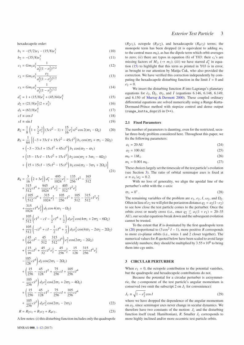
which reproduces the precession period for Ω2 seen in the sampleevolution of Figure 2 to within a factor of 3. The scaling factors in(36) are more reliable than the overall magnitude; the dependencieson m0, m1, a1, and a2 can be used to scale the time coordinate of onenumerical computation to another. Figure 2 is made for a particle inthe inverse Kozai resonance; note how the oscillation periods forω2,and by extension I and q2, are each a few dozen times longer thanthe nodal precession period. This is expected since for the inverseKozai resonance, dω2/dt vanishes at quadrupole order, leaving thehexadecapole contribution, which is smaller by ∼(a1/a2)2 = 1/25,dominant.

As shown in Figure 2, the secular trajectory within the ω2resonance is confirmed qualitatively by the N-body symplectic in-tegrator WHFast (Rein & Tamayo 2015; Wisdom & Holman 1991),part of the REBOUND package (version 3.5.8; Rein & Liu 2012). Atimestep of 0.25 yr was used (0.28% of the orbital period of theinterior perturber) for the N-body integration shown; it took lessthan 3 wall-clock hours to complete the 5 Gyr integration using a2.2 GHz Intel Core i7 processor on a 2015 MacBook Air laptop.

3.1.2 Inverse Kozai vs. Kozai

In the top panel of Figure 3, we show analogues to the “Kozai curves”made by Lithwick & Naoz (2011) for the conventional problem.This top panel delineates the allowed values of test particle eccen-tricity and inclination for given Jz and R when e1 = 0. Contrastthese “inverse Kozai curves” with the Kozai curves calculated byLithwick & Naoz (2011) in their Figure 2 (left panel): for the in-verse problem, the range of allowed eccentricities and inclinationsis much more restricted (at fixed Jz and R) than for the conventionalproblem. For the inverse problem when e1 = 0, e2 and I are strictlyconstant at quadrupole order; variations in e2 and I for the caseof a circular perturber are possible starting only at hexadecapoleorder, via the small inverse Kozai resonant term in R proportionalto e2

2 cos 2ω2 (variations in ω2 directly drive the variations in e2and I when e1 = 0). By comparison, in the conventional problem,variations in test particle eccentricity and inclination are possibleeven at quadrupole order, and large.

MNRAS 000, 1–12 (2017)


20

30

40

50

60

70

80

90

100

90 180 270

11.9°

36.8°

q2 (

AU

)

ω2 (deg)

Jz = 0.8

90 180 270

35.3°

62.6°

ω2 (deg)

Jz = 0.46

90 180 270

36.2°

63.0°

ω2 (deg)

Jz = 0.45

90 180 270

36.9°

63.2°

ω2 (deg)

Jz = 0.44

90 180 270

37.6°

63.3°

ω2 (deg)

Jz = 0.425

90 180 270

69.9°

78.5°

I min

Im

ax

ω2 (deg)

Jz = 0.2

Figure 1. Periastron distances q2 vs. arguments of periastron ω2, for e1 = 0. Because the potential presented by a circular perturber is axisymmetric,

Jz =

√

1 − e22 cos I is conserved; trajectories in a given panel have Jz as annotated. For given Jz , the inclination I increases monotonically but not linearly

with q2; the maximum and minimum inclinations for the trajectories plotted are labeled on the right of each panel. In a narrow range of Jz = 0.425–0.45 (forour chosen α = a1/a2 = 0.2), the inverse Kozai (a.k.a. ω2) resonance appears, near I ≃ 63.

30

40

50

60

70

80

90

100

q2 (

AU

)

SecularN−Body

61

62

63

64

I (d

eg)

30

60

90

120

150

ω2

(deg)

−360

−270

−180

−90

0

0 1×109

2×109

3×109

4×109

5×109

Ω2

(deg)

t (yrs)

Figure 2. Time evolution within the inverse Kozai resonance. The trajectorychosen is the one in Figure 1 with Jz = 0.45 and the largest librationamplitude. The nodal (Ω2) precession arises from the quadrupole potentialand is therefore on the order of 1/α2 ∼ 25 times faster than the librationtimescale for ω2, which is determined by the hexadecapole potential. Initialconditions: 2 = 90, Ω2 = 0, q2 = 87.5 AU, I = 63. Overplotted in reddashed lines are the results of an N -body integration with identical initialconditions (and initial true anomalies f1 = 0 and f2 = 180) inputted asJacobi coordinates. The N -body integration is carried out using WHFast

within the REBOUND package (Rein & Tamayo 2015; Wisdom & Holman1991).

This key difference between the conventional and inverse prob-lems stems from the difference between the interior and exterior ex-pansions of the 1/∆ potential. The conventional interior expansioninvolves the sum Pℓrℓtest, where Pℓ is the Legendre polynomial of

order ℓ and rtest is the radial position of the test particle. The inverse

exterior expansion involves a qualitatively different sum, Pℓr−(ℓ+1)test .

The time-averaged potentials in the conventional and inverse prob-lems therefore involve different integrals; what averages to a termproportional to cos(2ωtest) in the conventional quadrupole problemaverages instead in the inverse problem to a constant, independent ofthe test particle’s argument of periastron ωtest (we have verified thislast statement by evaluating these integrals). An interior multipolemoment of order ℓ is not the same as an exterior multipole momentof the same order. We could say that the inverse exterior poten-tial looks “more Keplerian” insofar as its monopole term scales as1/rtest.

4 ECCENTRIC PERTURBER

When e1 , 0, all orders (quadrupole, octopole, and hexadecapole)contribute to the potential seen by the test particle. The potentialis no longer axisymmetric, and so Jz is no longer conserved. Thisopens the door to orbit “flipping”, i.e., a prograde (I < 90) orbit canswitch to being retrograde (I > 90) and vice versa (e.g., Naoz et al.2017). There is only one constant of the motion, R.

4.1 First Survey

Whereas when e1 = 0 the evolution did not depend on Ω2, itdoes when e1 , 0. For our first foray into this large multi-dimensional phase space, we divided up initial conditions as follows.For each of four values of e1 ∈ 0.03, 0.1, 0.3, 0.7, we scannedsystematically through different initial values of q2,init (equiva-lently e2,init) ranging between a2 = 100 AU and a1 = 20 AU.For each q2,init, we assigned Iinit according to one of three val-

ues of Jz,init ≡√

1 − e22,init cos Iinit ∈ 0.8, 0.45, 0.2, representing

“low”, “intermediate”, and “high” inclination cases, broadly speak-ing. Having set e1, q2,init(e2,init), and Jz,init(Iinit), we cycled throughfive values of 2,init ∈ 0, 45, 90, 135, 180 and three valuesof ω2,init ∈ 0, 90, 270.

We studied all integrations from this large ensemble, addingmore with slightly different initial conditions as our curiosity ledus. In what follows, we present a subset of the results from this firstsurvey, selecting those we thought representative or interesting.Later, in Section 4.2, we will provide a second and more thoroughsurvey using surfaces of section. A few sample integrations from

MNRAS 000, 1–12 (2017)

6 Vinson & Chiang

30

60

90

120

150

180

Jz = 0.45

Jz = −0.45

0.447

−0.447

0.425

−0.425

e1 = 0

I (d

eg

)

R = −0.05032

30

60

90

120

150

I (d

eg

)

e1 = 0.1

30

60

90

120

150

0 0.1 0.2 0.3 0.4 0.5 0.6 0.7 0.8

I (d

eg

)

e2

e1 = 0.3

Figure 3. Inclination I vs. eccentricity e2 for a constant disturbing functionR = −0.05032 (see section 2.1 for the units of R). When e1 = 0, Jz is anadditional constant of the motion; the resultant “inverse Kozai curves” (toppanel) for our external test particle are analogous to the conventional “Kozaicurves” shown in Figure 2 of Lithwick & Naoz (2011) for an internal testparticle. Compared to the conventional case, the ranges of I and e2 in theinverse case are much more restricted; what variation there is is only possiblebecause of the e2

2 cos(2ω2) term that appears at hexadecapolar order (seeequation 22). As e1 increases above zero (middle and bottom panels), Jzvaries more and variations in I grow larger. In each of the middle and bottompanels, points are generated by integrating the equations of motion for sixsets of initial conditions specified in Table A1.

both surveys will be tested against N-body calculations in Section4.3 (see also Figure 2).

4.1.1 Low Perturber Eccentricity e1 ≤ 0.1

Comparison of Figure 4 with Figure 1 shows that at low perturbereccentricity, e1 . 0.1, the test particle does not much change itsbehavior from when e1 = 0 (for a counter-example, see Figure 6).

30

40

50

60

70

80

90

100

q2 (

AU

)

Jz,init = 0.8

I I I I I I I I I I I

Jz,init = 0.45

II I I I I II

I II I I

II

Jz,init = 0.2

IIIII

II

III

III

II

0

15

30

45

60

75

90

90 180 270

I (d

eg

)

ω2 (deg)

I I I I I I I I I I I

90 180 270

ω2 (deg)

II I I I I I II I

II I I

I

90 180 270 360

ω2 (deg)

IIIII

III

III

III

I

Figure 4. Analogous to Figure 1, but now for a mildly eccentric perturber(e1 = 0.1). Because e1 , 0, Jz is not conserved and cannot be used toconnect q2 and I uniquely; we have to plot q2 and I in separate panels.Nevertheless, e1 is still small enough that Jz is approximately conserved;q2 and I still roughly follow one another for a given Jz, init, i.e., the familyof trajectories proceeding from lowest I (marked by vertical bars) to highestI corresponds to the same family of trajectories proceeding from lowest q2

(marked by vertical bars) to highest q2. The ω2 resonance can still be seennear I ≃ 63, in the center panels for Jz, init = 0.45. All the non-resonanttrajectories are initialized with 2 = 0 and ω2 = 0. For the four resonanttrajectories, the initial 2 = 0 and ω2 = ±90.

The same inverse Kozai resonance appears for Jz,init = 0.45 ande1 = 0.1 as it does for e1 = 0. The maximum libration amplitude ofthe resonance is somewhat higher at the larger e1. The trajectoriesshown in Figure 4 are for 2,init = 0, but qualitatively similarresults obtain for other choices of 2,init.

The middle panel of Figure 3 elaborates on this result, showingthat even though Jz,init is not strictly conserved when e1 , 0, it canbe approximately conserved (again, see the later Figure 6 for acounter-example). Test particles explore more of e2-I space whene1 = 0.1 than when e1 = 0, but they still largely respect (for thespecific R of Figure 3) the constraints imposed by Jz when e1 = 0.This statement also holds at e1 = 0.3 (lower panel), but to a lesserextent.

Figure 5 illustrates how the hexadecapole (hex) potential—specifically the inverse Kozai resonance—can qualitatively changethe test particle dynamics at octopole (oct) order. Only at hex orderis the ω2 resonance evident. Compared to the oct level dynamics,the periastron distance q2 varies more strongly, hitting its maximumand minimum values atω2 = 90 or 270 (instead of at 0 and 180,as an oct treatment would imply).

Orbit flipping becomes possible when e1 , 0, for sufficientlylarge I or e2 (Naoz et al. 2017). Figure 6 is analogous to Figure3 except that it is made for a more negative R, corresponding tolarger I (insofar as R is dominated by the quadrupole term). Forthis R = −0.1373, as with the previous R = −0.05032, e2 and I

hardly vary when e1 = 0 (Section 3.1.2). But when e1 = 0.1, theconstraints imposed by fixed Jz come loose; Figure 6 shows that asingle particle’s Jz can vary dramatically from positive (prograde)to negative (retrograde) values. As shown by Naoz et al. (2017, seetheir Figure 1), such orbit flipping is possible even at quadrupoleorder; flipping is not associated with the ω2 resonance, but rather

MNRAS 000, 1–12 (2017)


20

40

60

80

100

90 180 270

q2 (

AU

)

ω2 (deg)

Quad

90 180 270

ω2 (deg)

Oct

90 180 270

ω2 (deg)

Hex

0

15

30

45

60

75

90

90 180 270

I (d

eg

)

Ω2 (deg)90 180 270

Ω2 (deg)90 180 270

Ω2 (deg)

Figure 5. Comparing quadrupole (quad), octopole (oct), and hexadecapole(hex) evolutions for e1 = 0.1 and the same test particle initial conditions(e2 = 0.2, I = 62.66, 2 = 0, and ω2 = 90). The hex panel features asecond set of initial conditions identical to the first except that ω2 = 270;the two hex trajectories map to the same quad and oct trajectories as shown.The inverse Kozai resonance, featuring libration of ω2 about ±90 and∼20% variations in e2, appears only in a hex-level treatment.

with librations of Ω2 about 90 or 270 (where 1 = 0 defineszero longitude). We verify the influence of this “Ω2 resonance” inthe middle panel of Figure 6.

4.1.2 High Perturber Eccentricity e1 = 0.3, 0.7

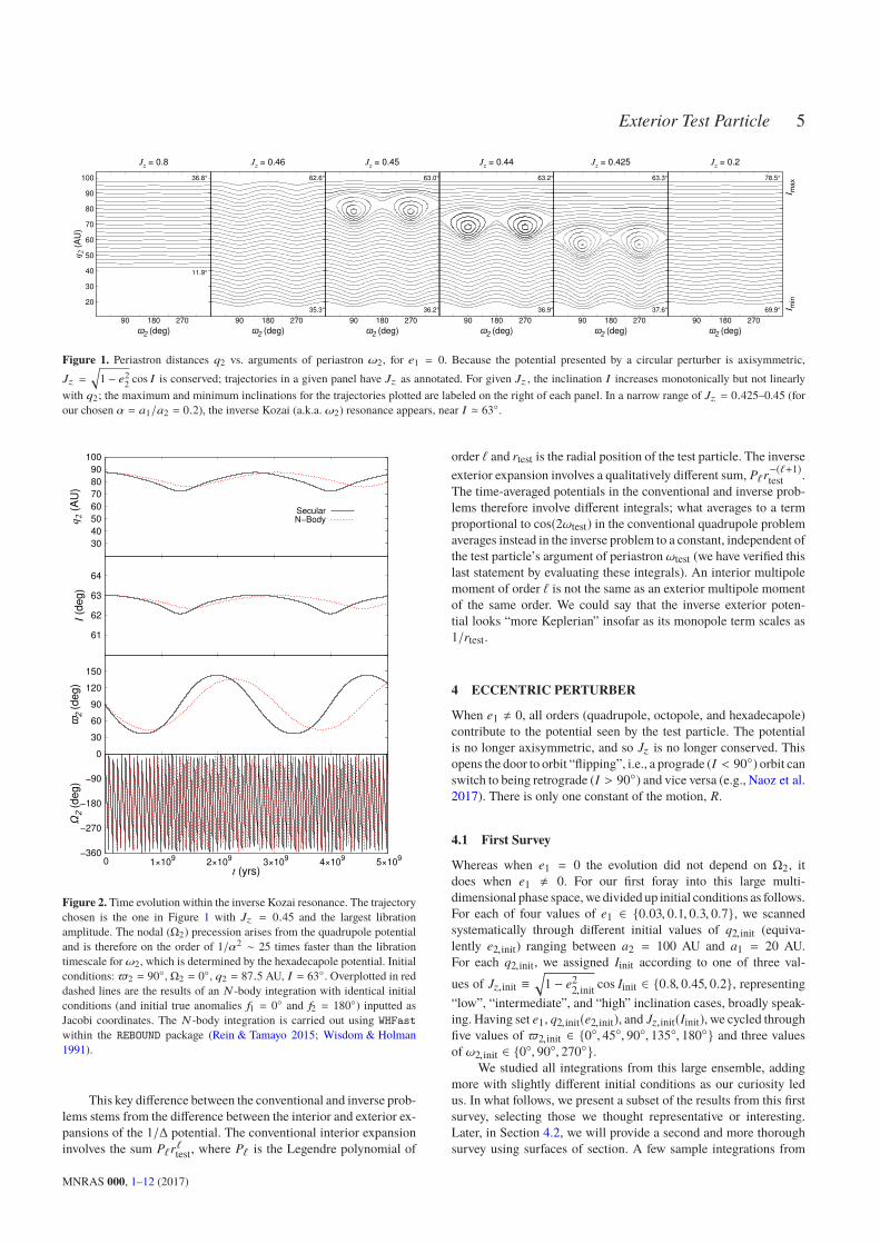
We highlight a few comparisons between an oct level treatmentand a hex level treatment. We begin with Figure 7 which showspractically no difference. Many of the integrations in our first surveyshowed no significant difference in going from oct to hex. We alsotested some of the cases showcased in Naoz et al. (2017) and foundthat including the hex dynamics did not substantively alter theirevolution.

Cases where the hex terms matter are shown in Figures 8–11.The ω2 resonance, seen only at hex order, can stabilize the motion;in Figure 8, the ω2 resonance eliminates the chaotic variations seenat the oct level in q2 and I. Even when theω2 resonance is not active,hex level terms can dampen eccentricity and inclination variations(Figures 9 and 10). But the hex terms do not necessarily suppress;in Figure 11 they are seen to nudge the test particle from a progradeto a retrograde orbit, across the separatrix of the Ω2 resonance.

4.2 Second Survey: Surfaces of Section

Surfaces of section (SOS’s) afford a more global (if also more ab-stract) view of the dynamics. By plotting the test particle’s positionin phase space only when one of its coordinates periodically equalssome value, we thin its trajectory out, enabling it to be comparedmore easily with the trajectories of other test particles with dif-ferent initial conditions. In this lower dimensional projection, it isalso possible to identify resonances, and to distinguish chaotic fromregular trajectories.

Since we are particularly interested in seeing how ω2 andits quasi-conjugate e2 behave, we section using Ω2, plotting the

0

30

60

90

120

150

180

0 0.1 0.2 0.3 0.4 0.5 0.6 0.7 0.8

e1 = 0.1

0.3

−0.3

0.2

−0.2

0.1

−0.1

e1 = 0, Jz = 0

I (d

eg

)

e2

R = −0.1373

0

30

60

90

120

150

180

0 60 120 180 240 300 360

e1 = 0.1

I (d

eg

)

Ω2 (deg)

20

30

40

50

60

70

80

90

100

0 60 120 180 240 300 360

e1 = 0.1

q2 (

AU

)

ω2 (deg)

Figure 6. Top panel: Inclination I vs. eccentricity e2 for a fixed disturbingfunction R = −0.1373 (see Section 2.1 for the units of R). Different coloredpoints, corresponding to different Jz values as marked, are for e1 = 0, andare analogous to those shown in the top panel of Figure 3. The black pointsrepresent the trajectory of a single test particle, integrated for e1 = 0.1 andusing the following initial conditions: e2 = 0.3691, I = 85, 2 = 0,and Ω2 = 0. When e1 , 0, Jz is no longer conserved, and e2 and I varydramatically for this value of R; Jz even changes sign as the orbit flips.The variation in e2 is so large that eventually the test particle crosses theorbit of the perturber (e2 > 0.8), at which point we terminate the trajectory.Center panel: Inclination I vs. longitude of ascending node Ω2 for the sameblack trajectory shown in the top panel. The two lobes of the Ω2 resonance(Naoz et al. 2017) are evident, around which the particle lingers. Bottompanel: The same test particle trajectory shown in black for the top andmiddle panels, now in e2 vs. ω2 space. The evolution is evidently chaotic.

MNRAS 000, 1–12 (2017)

8 Vinson & Chiang

20

30

40

50

60

70

80

90

100

90 180 270

q2 (

AU

)

ω2 (deg)

Quad

90 180 270

ω2 (deg)

Oct

90 180 270

ω2 (deg)

Hex

0

30

60

90

120

150

180

90 180 270

I (d

eg

)

Ω2 (deg)90 180 270

Ω2 (deg)90 180 270

Ω2 (deg)

Figure 7. Analogous to Figure 5, but for e1 = 0.3 and the following testparticle initial conditions: e2 = 0.2, I = 62.66, Ω2 = ±90, 2 = 0.The two test particle trajectories overlap in q2-ω2 space (top panels). Forthese initial conditions, the Ω2 resonance (Naoz et al. 2017) appears at allorders quad through hex (bottom panels). The oct and hex trajectories appearqualitatively similar in all respects.

20

30

40

50

60

70

80

90

100

90 180 270

q2 (

AU

)

ω2 (deg)

Quad

90 180 270

ω2 (deg)

Oct

90 180 270

ω2 (deg)

Hex

0

30

60

90

120

150

180

90 180 270

I (d

eg

)

Ω2 (deg)90 180 270

Ω2 (deg)90 180 270

Ω2 (deg)

Figure 8. Analogous to Figure 5, but for e1 = 0.3 and the following testparticle initial conditions: e2 = 0.55, I = 57.397, Ω2 = 45 and 225,2 = 135. The inverse Kozaiω2 resonance is visible in the hex panels only,with a more widely varying inclination here for e1 = 0.3 than for e1 = 0(compare with Figure 5). The phase space available to the ω2 resonanceshrinks with increasing e1; at e1 = 0.7, we could not find the resonance(see Figure 14). Two test particle trajectories are displayed for the hex panel;since they overlap at the quad and oct levels, only one trajectory is shownfor those panels (the one for which the initial Ω2 = 45).

particle’s position in q2-ω2 space and I-ω2 space whenever Ω2 =

180 (with zero longitude defined by 1 = 0). We have verifiedin a few cases that the trajectories so plotted trace the maximumand minimum values of q2 and I; our SOS’s contain the boundingenvelopes of the trajectories.

Figure 12 shows Ω2-SOS’s for e1 = 0.1 and a sequence of

20

30

40

50

60

70

80

90

100

90 180 270

q2 (

AU

)

ω2 (deg)

Quad

90 180 270

ω2 (deg)

Oct

90 180 270

ω2 (deg)

Hex

0

30

60

90

120

150

180

90 180 270

I (d

eg

)

Ω2 (deg)90 180 270

Ω2 (deg)90 180 270

Ω2 (deg)

Figure 9. Analogous to Figure 5, but for e1 = 0.3 and the following testparticle initial conditions: e2 = 0.15, I = 62.925, Ω2 = 45 and 225,2 = 135. Two test particle trajectories are displayed for the hex panel;since they overlap at the quad and oct levels, only one trajectory is shownfor those panels (the one for which the initial Ω2 = 225). The hex potentialsuppresses the eccentricity variation seen at the oct level, and removes theparticle from the separatrix of theΩ2 resonance, bringing it onto one of twoislands of libration.

20

30

40

50

60

70

80

90

100

90 180 270

q2 (

AU

)

ω2 (deg)

Quad

90 180 270

ω2 (deg)

Oct

90 180 270

ω2 (deg)

Hex

0

30

60

90

120

150

180

90 180 270

I (d

eg

)

Ω2 (deg)90 180 270

Ω2 (deg)90 180 270

Ω2 (deg)

Figure 10. Analogous to Figure 5, but for e1 = 0.7 and the following testparticle initial conditions: e2 = 0.525, I = 58.081, Ω2 = 135 and 315,2 = 135. As with Figures 8 and 9, the hex potential helps to stabilize themotion; here it locks the particle to one of two librating islands of the Ω2

resonance and prevents the orbit crossing seen at the oct level.

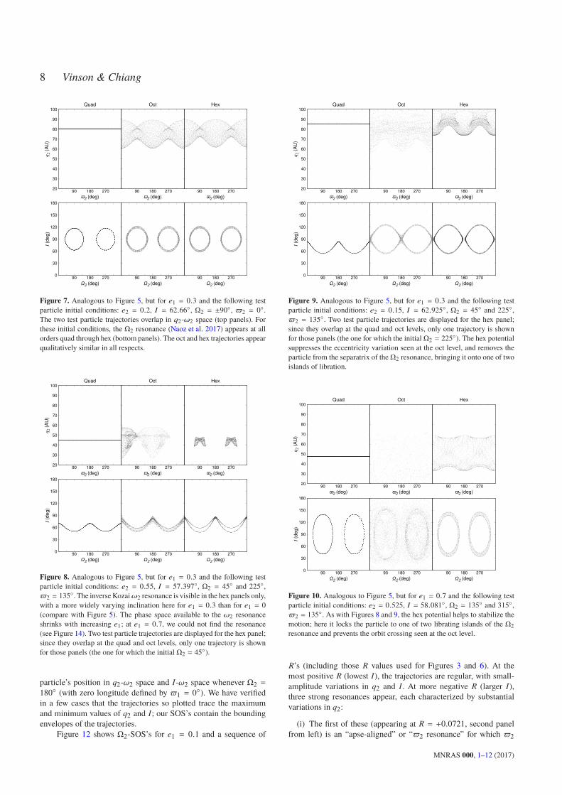
R’s (including those R values used for Figures 3 and 6). At themost positive R (lowest I), the trajectories are regular, with small-amplitude variations in q2 and I. At more negative R (larger I),three strong resonances appear, each characterized by substantialvariations in q2:

(i) The first of these (appearing at R = +0.0721, second panelfrom left) is an “apse-aligned” or “2 resonance” for which 2

MNRAS 000, 1–12 (2017)


20

30

40

50

60

70

80

90

100

90 180 270

q2 (

AU

)

ω2 (deg)

Quad

90 180 270

ω2 (deg)

Oct

90 180 270

ω2 (deg)

Hex

0

30

60

90

120

150

180

90 180 270

I (d

eg

)

Ω2 (deg)90 180 270

Ω2 (deg)90 180 270

Ω2 (deg)

Figure 11. Analogous to Figure 5, but for e1 = 0.7 and the following testparticle initial conditions: e2 = 0.1, I = 84.232, Ω2 = 180, 2 = 180.Here the hex potential nudges the particle from a circulating trajectory ontothe separatrix of the Ω2 resonance (contrast with Figures 9 and 10).

librates about 0 and

I(2−res) ≃ arccos

(

+1 ±√

6

5

)

≃ 46 and 107 . (37)

At these inclinations, by equation (35), d2/dt |quad,e1=0 = 0.4

(ii) The second of the resonances (R = −0.0721, two lobes inthe middle panel) is the inverse Kozai or ω2 resonance, appearingat I(ω2−res) ≃ 63 and 117, for which ω2 librates about ±90

(Section 3.1).(iii) The third resonance (R = −0.0721, −0.0938, and −0.1373;

middle, fourth, and fifth panels) appears at

I(ω2−Ω2−res) ≃ arccos

(

−1 ±√

6

5

)

≃ 73 and 134 , (38)

inclinations for which Ûω2 = ÛΩ2 (equations 31 and 34). We refer tothis last resonance as the “ω2 −Ω2 resonance”. The resonant anglelibrates about 0.

For the above three resonances, we have verified that theirrespective resonant arguments (2; ω2; ω2 − Ω2) librate (see alsoFigure 15), and have omitted their retrograde branches from theSOS for simplicity. The ω2 − Ω2 and 2 resonances appear atoctopole order; they are associated with the first two terms in theoctopole disturbing function (21), respectively. The ω2 resonanceis a hexadecapolar effect, as noted earlier.

The SOS for e1 = 0.3 (Figure 13) reveals dynamics qualita-tively similar to e1 = 0.1, but with larger amplitude variations inq2. We have verified in Figure 13 that the island of libration seenat R = 0.0503 is the 2 resonance; the islands near the top of thepanels for R = 0 and −0.0503 represent the ω2 −Ω2 resonance; and

4 The apse-aligned resonance identified here is at small α and large I ≃46/107, but another apse-aligned resonance also exists for orbits that areco-planar or nearly so (e.g., Wyatt et al. 1999). The latter can be found usingLaplace-Lagrange secular theory, which does not expand in α but rather ineccentricity and inclination.

the two islands centered on ω2 = ±90 at R = −0.0503 representthe inverse Kozai resonance. For both e1 = 0.3 and 0.1, chaos ismore prevalent at more negative R / larger I. The chaotic trajectoriesdip to periastron distances q2 near a1 = 20 AU, and in Figure 12 weshow a few that actually cross orbits with the perturber. Once orbitscross, the subsequent secular evolution can no longer be trusted,but we have plotted the orbit-crossing trajectories anyway just todemonstrate that channels exist whereby test particle periastra canbe lifted from near the perturber to substantially larger distances.

At e1 = 0.7 (Figure 14) we find, in addition to the2 resonanceat R ≤ 0.4, a new resonance at R ≥ 0.5. For this latter resonance,ω2 + 3Ω2 librates about 0. Although this resonance is found atoctopole order—it is embodied in the fourth term in equation (21)—we found by experimentation that eliminating the hexadecapolecontribution to the disturbing function removes the test particle fromthis resonance (for the same initial conditions as shown in Figure14). Evidently the hexadecapole potential helps to enforce Ûω2 =

−3 ÛΩ2 so that this octopole resonance can be activated. Remarkably,this “ω2+3Ω2 resonance” enables the test particle to cycle betweena nearly (but not exactly) co-planar orbit to one inclined by ∼60–70, while having its eccentricity e2 vary between ∼0.2–0.6. Wewill see in Section 4.3, however, that a full N-body treatment mutesthe effects of this resonance.

4.3 N-Body Tests

Having identified five resonances in the above surveys, we test theirrobustness using N-body integrations. We employ the WHFast sym-plectic integrator (Rein & Tamayo 2015; Wisdom & Holman 1991),part of the REBOUND package (Rein & Liu 2012), adopting timestepsbetween 0.1–0.25 yr. Initial conditions (inputted for the N-body ex-periments as Jacobi elements, together with initial true anomaliesf1 = 0 and f2 = 180) were drawn from the above surveys with thegoal of finding resonant libration at as large a perturber eccentricitye1 as possible. In Figure 15 we verify that the ω2, Ω2, 2, andω2 − Ω2 resonances survive a full N-body treatment when e1 is ashigh as 0.1, 0.7, 0.7, and 0.1, respectively (see also Figure 2). TableA5 records the initial conditions.

We were unable in N-body calculations to lock the test parti-cle into the ω2 + 3Ω2 resonance, despite exploring the parameterspace in the vicinity where we found it in the secular surfaces ofsection. This is unsurprising insofar as we had found this resonanceto depend on both octopole and hexadecapolar effects at the largestperturber eccentricity tested, e1 = 0.7; at such a high eccentricity,effects even higher order than hexadecapole are likely to be signif-icant, and it appears from our N-body calculations that they are,preventing a resonant lock. We show in Figure 15 an N-body tra-jectory that comes close to being in the ω2 + 3Ω2 resonance (onaverage, Ûω2 ≈ −2.7 ÛΩ2). Although the inclination does not vary asdramatically as in the truncated secular evolution, it can still cyclebetween ∼20 and 70.

5 SUMMARY

We have surveyed numerically the dynamics of an external test par-ticle in the restricted, secular, three-body problem. We wrote downthe secular potential of an internal perturber to hexadecapolar or-der (where the expansion parameter is the ratio of semimajor axesof the internal and external bodies, α = a1/a2 < 1) by adapt-ing the disturbing function for an external perturber as derived by

MNRAS 000, 1–12 (2017)

10 Vinson & Chiang

20

40

60

80

100

q2 (

AU

)

R = 0.3000 R = 0.0721 R = −0.0721 R = −0.0938 R = −0.1373

0

15

30

45

60

75

90

90 180 270

I (d

eg)

ω2 (deg)90 180 270

ω2 (deg)90 180 270

ω2 (deg)90 180 270

ω2 (deg)90 180 270

ω2 (deg)

Figure 12. Surfaces of section (SOS’s) for perturber eccentricity e1 = 0.1 and various values of the disturbing function R (the only constant of the motionwhen e1 , 0; see Section 2.1 for the units of R) labeled at the top of the figure. These SOS’s are sectioned using Ω2: a point is plotted every time Ω2 crosses180. Each test particle trajectory is assigned its own color; see Table A2 in the Appendix for the initial conditions. At R = 0.072, the 2 resonance appears. AtR = −0.0721, the ω2 (inverse Kozai) resonance appears (dark blue and turquoise lobes centered on ω2 = ±90). At R = 0, −0.0938, and −0.1373, the ω2 −Ω2

resonance manifests (this angle librates about 0). These three resonances are accessed at inclinations I ∼ 45–75 (and at analogous retrograde inclinationsthat are not shown). The region at large q2 for R = −0.1373 is empty because here the test particle locks into the Ω2 resonance studied by Naoz et al. (2017),in which Ω2 librates about 90 and so does not trigger our sectioning criterion.

Yokoyama et al. (2003, Y03). In making this adaptation, we cor-rected a misprint in the hexadecapolar potential of Y03 (M. Ćuk2017, personal communication). Our numerical survey was con-ducted at fixed α = 0.2.

Inclination variations for an external test particle can be dra-matic when the eccentricity of the internal perturber e1 is non-zero.The variations in mutual inclination I are effected by a quadrupoleresonance for which Ω2, the test particle’s longitude of ascend-ing node (referenced to the perturber’s orbit plane, with longitudezero pointing toward the perturber’s periapse), librates about ±90.Within the Ω2 resonance, the test particle’s orbit flips (switchesfrom prograde to retrograde). Flipping is easier—i.e., the minimumI for which flipping is possible decreases—with increasing e1. Allof this inclination behavior was described by Naoz et al. (2017) andwe have confirmed these essentially quadrupolar results here.

Eccentricity variations for an external test particle rely on oc-topole or higher-level effects (at the quadrupole level of approxi-mation, the test particle eccentricity e2 is strictly constant). Whene1 = 0, octopole effects vanish, and the leading-order resonanceable to produce eccentricity variations is the hexadecapolar “inverseKozai resonance” in which the test particle’s argument of perias-tron ω2 librates about ±90 (Gallardo et al. 2012). The resonancedemands rather high inclinations, I ≃ 63 or 117. By comparisonto its conventional Kozai counterpart which exists at quadrupoleorder, the hexadecapolar inverse Kozai resonance is more restricted

in scope: it exists only over a narrow range of Jz =

√

1 − e22 cos I

for a given α, and produces eccentricity variations on the order of

∆e2 ≃ 0.2. In our truncated secular treatment, we found the inverseKozai resonance to persist up to perturber eccentricities of e1 = 0.3;in N-body experiments, we found the resonance up to e1 = 0.1. Athigher e1, the hexadecapolar resonance seems to disappear, over-whelmed by octopole effects.

Surfaces of section made for e1 , 0 and Ω2 = 180 revealedtwo octopole resonances characterized by stronger eccentricity vari-ations of ∆e2 up to 0.5. The resonant angles are the longitude ofperiapse 2, which librates about 0, and ω2 − Ω2, which alsolibrates about 0. The 2 and ω2 − Ω2 resonances are like the in-verse Kozai resonance in that they also require large inclinations,I ≃ 46/107 and 73/134, respectively. The apse-aligned2 res-onance survives full N-body integrations up to e1 = 0.7; theω2−Ω2resonance survives up to e1 = 0.1. At large e1, the requirement onI for the 2 resonance lessens to about ∼20.

We identified two rough, qualitative trends: (1) the larger e1is, the more the eccentricity and inclination of the test particle canvary; and (2) the more polar the test particle orbit (i.e., the closer I

is to 90), the more chaotic its evolution.

This paper is but an initial reconnaissance of the external testparticle problem. How the various resonances we have identifiedmay have operated in practice to shape actual planetary/star systemsis left for future study. One aspect of the problem we need to exploreare the effects of general relativity (GR). For our chosen parameters,GR causes the periapse of the perturber to precess at a rate that istypically several hundreds of times slower than the rate at which thetest particle’s node precesses. Such an additional apsidal precession

MNRAS 000, 1–12 (2017)


20

40

60

80

100

q2 (

AU

)

R = 0.3000 R = 0.0503 R = 0.0000 R = −0.0503 R = −0.0721

0

15

30

45

60

75

90

90 180 270

I (d

eg)

ω2 (deg)90 180 270

ω2 (deg)90 180 270

ω2 (deg)90 180 270

ω2 (deg)90 180 270

ω2 (deg)

Figure 13. Same as Figure 12 but for e1 = 0.3. The 2 resonance appears at R = 0.0503; the ω2 − Ω2 resonance appears at R = 0 and −0.0503; and thedouble-lobed inverse Kozai resonance appears at R = −0.0503. Initial conditions used to make this figure are in Table A3.

20

40

60

80

100

q2 (

AU

)

R = 0.5500 R = 0.5000 R = 0.4000 R = 0.3000 R = 0.2650

0

15

30

45

60

75

90

90 180 270

I (d

eg)

ω2 (deg)90 180 270

ω2 (deg)90 180 270

ω2 (deg)90 180 270

ω2 (deg)90 180 270

ω2 (deg)

Figure 14. Same as Figure 12 but for e1 = 0.7. In addition to the 2 resonance at R ≤ 0.4, a new resonance appears at R ≥ 0.5 for which ω2 + 3Ω2 libratesabout 0. This last resonance, however, is not found in full N -body integrations (by contrast to the other four resonances identified in this paper; see Figure15). Initial conditions used to make this figure are in Table A4.

MNRAS 000, 1–12 (2017)

12 Vinson & Chiang

20

30

40

50

60

70

80

90

100

q2 (

AU

)

N−BodySecular

30

60

90

120

150

I (d

eg)

−180

−120

−60

0

60

120

2×108

5×108

8×108

(a) ω2

resonant angle

(deg)

5×106

1.5×107

2.5×107

(b) Ω2

2×108

5×108

8×108

(c) ϖ2

t (yrs) 2×10

8 5×10

8 8×10

8

(d) ω2 − Ω2

5×106

1.5×107

2.5×107

(e) ω2 + 3Ω2

Figure 15. Comparison of N -body (dashed red) vs. secular (solid black) integrations. Initial conditions, summarized in Table A5, are chosen to lock the testparticle into the ω2, Ω2, 2, and ω2 −Ω2 resonances (panels a through d). We failed to obtain a lock for the ω2 + 3Ω2 resonance in our N -body calculationsand offer an instead an N -body trajectory that comes close to librating ( Ûω2 ≈ −2.7 ÛΩ2; panel e), together with its secular counterpart which does appear tolibrate.

is not expected to affect our results materially; still, a check shouldbe made. A way to do that comprehensively is to re-compute oursurfaces of section with GR.

ACKNOWLEDGEMENTS

We are grateful to Edgar Knobloch and Matthias Reinsch for teach-ing Berkeley’s upper-division mechanics course Physics 105, andfor connecting BV with EC. This work was supported by a BerkeleyExcellence Account for Research and the NSF. Matija Ćuk alertedus to the misprint in Y03 and provided insights that were most help-ful. We thank Konstantin Batygin, Eve Lee, and Yoram Lithwickfor useful discussions, and Daniel Tamayo for teaching us how touse REBOUND.

REFERENCES

Bailey M. E., Chambers J. E., Hahn G., 1992, Astronomy and Astrophysics,257, 315

Carruba V., 2002, Icarus, 158, 434Gallardo T., Hugo G., Pais P., 2012, Icarus, 220, 392Kozai Y., 1962, The Astronomical Journal, 67, 591Kushnir D., Katz B., Dong S., Livne E., Fernández R., 2013, The Astro-

physical Journal, 778, L37Lee E. J., Chiang E., 2016, The Astrophysical Journal, 827, 125Lidov M. L., 1962, Planetary and Space Science, 9, 719Lithwick Y., Naoz S., 2011, The Astrophysical Journal, 742, 94Murray C. D., Dermott S. F., 2000, Solar System Dynamics. ”Cambridge

University Press”

Naoz S., Farr W. M., Lithwick Y., Rasio F. A., Teyssandier J., 2011, Nature,473, 187

Naoz S., Li G., Zanardi M., de Elía G. C., Di Sisto R. P., 2017, The Astro-nomical Journal, 154, 18

Nesvold E. R., Naoz S., Vican L., Farr W. M., 2016, The AstrophysicalJournal, 826, 19

Nesvorny D., Alvarellos J. L. A., Dones L., Levison H. F., 2003, The Astro-nomical Journal, 126, 398

Pearce T. D., Wyatt M. C., 2014, Monthly Notices of the Royal AstronomicalSociety, 443, 2541

Rein H., Liu S.-F., 2012, A&A, 537, A128Rein H., Tamayo D., 2015, MNRAS, 452, 376Sheppard S. S., Trujillo C., 2016, The Astronomical Journal, 152, 221Silsbee K., Tremaine S., 2016, The Astronomical Journal, 152, 103Silsbee K., Tremaine S., 2017, The Astrophysical Journal, 836, 39Thomas F., Morbidelli A., 1996, Celestial Mechanics, 64, 209Tremaine S., Yavetz T. D., 2014, American Journal of Physics, 82, 769Wisdom J., Holman M., 1991, AJ, 102, 1528Wu Y., Murray N., 2003, The Astrophysical Journal, 589, 605Wyatt M. C., Dermott S. F., Telesco C. M., Fisher R. S., Grogan K., Holmes

E. K., Piña R. K., 1999, The Astrophysical Journal, 527, 918Yokoyama T., Santos M. T., Cardin G., Winter O. C., 2003, Astronomy and

Astrophysics, 401, 763Zanardi M., de Elía G. C., Di Sisto R. P., Naoz S., Li G., Guilera O. M.,

Brunini A., 2017, Astronomy and Astrophysics, 605, A64

APPENDIX A: INITIAL CONDITIONS

This paper has been typeset from a TEX/LATEX file prepared by the author.

MNRAS 000, 1–12 (2017)

http://dx.doi.org/10.1051/0004-6361/201118085

http://adsabs.harvard.edu/abs/2012A%26A...537A.128R

http://dx.doi.org/10.1093/mnras/stv1257

http://adsabs.harvard.edu/abs/2015MNRAS.452..376R

http://dx.doi.org/10.1086/115978

http://adsabs.harvard.edu/abs/1991AJ....102.1528W


Table A1. Initial conditions for Figure 3 (R = −0.05032).

e2 Ω2 2 I Jz, init

(rad) (rad) (rad)

Center Panel (e1 = 0.1, 1 = 0)

0.2110 0 1.5708 1.1170 0.42850.2110 0 1.5708 2.0246 -0.42850.4165 0 1.5708 1.0821 0.42680.4165 0 1.5708 2.0595 -0.42680.6738 0 0 1.0123 0.39160.6738 0 0 2.1293 -0.3916

Bottom Panel (e1 = 0.3, 1 = 0)

0.1094 0 1.5708 1.4486 0.12120.1094 0 1.5708 1.6930 -0.12120.5575 0 0 1.3264 0.20090.5575 0 0 1.8151 -0.20090.7061 0 0 1.3264 0.17130.7061 0 0 1.8151 -0.1713

Table A2. Initial conditions for Figure 12 (e1 = 0.1, 1 = 0).

color e2 Ω2 2 I

(rad) (rad) (rad)

R = 0.3000

black 0.3189 0.0000 0.0000 0.0175violet 0.3974 0.0000 0.0000 0.2443

red 0.5421 0.0000 0.0000 0.0454dark blue 0.4656 -0.7854 0.0000 0.3491turquoise 0.6604 -0.7854 0.0000 0.5934

R = 0.0721

black 0.0678 -0.7854 0.0000 0.7592violet 0.1894 -0.7854 0.0000 0.7679

red 0.3685 -0.7854 0.0000 0.7941dark blue 0.4556 -0.7854 0.0000 0.8116turquoise 0.6036 0.0000 0.0000 0.8465

blue 0.0957 -1.5708 0.0000 0.7505gray 0.6683 -1.5708 0.0000 0.8552

R = −0.0721

black 0.0072 -1.5708 0.0000 1.1519violet 0.5842 0.0000 0.0000 1.0821

red 0.2535 0.0000 0.3491 1.1868dark blue 0.4882 0.0000 0.9076 1.1170turquoise 0.4882 -3.1416 0.9076 1.1170

blue 0.3832 0.0000 1.3963 1.1519gray 0.1479 0.0000 1.4661 1.2042

yellow 0.2485 0.0000 1.5359 1.1868

R = −0.0938

black 0.0787 0.0000 0.0000 1.3177violet 0.1563 -0.7854 0.0000 1.2654

red 0.2028 -0.7854 0.0000 1.2566dark blue 0.2733 -0.7854 0.0000 1.2392turquoise 0.5353 0.0000 0.1396 1.1519

blue 0.3088 0.0000 0.4189 1.2566gray 0.5957 0.0000 0.6981 1.1170

yellow 0.4617 0.0000 1.3963 1.1868

R = −0.1373

black 0.3691 0.0000 0.0000 1.4835violet 0.3500 0.0000 0.3491 1.5533

red 0.4684 0.0000 0.6283 1.3439dark blue 0.3565 0.0000 0.8378 1.5185turquoise 0.3326 0.0000 0.2793 1.0996

blue 0.5176 0.0000 1.2566 1.2915

MNRAS 000, 1–12 (2017)

14 Vinson & Chiang


color e2 Ω2 2 I

(rad) (rad) (rad)

R = 0.3000

black 0.3207 0.0000 0.0000 0.2443violet 0.4371 0.0000 0.0000 0.4014

red 0.5534 -1.5708 0.0000 0.4712dark blue 0.6588 -1.5708 0.0000 0.6283turquoise 0.2110 -1.5708 0.0000 0.0175

R = 0.0503

black 0.3279 0.0000 0.0000 0.9948violet 0.4362 0.0000 0.0000 1.0123


blue 0.2608 -0.7854 0.0000 0.8552

R = 0.0000

black 0.2127 -0.7854 0.0000 0.9687violet 0.3300 -0.7854 0.0000 0.9774


R = −0.0503

black 0.3380 -0.7854 0.0000 1.0996violet 0.3380 -3.9270 0.0000 1.0996


blue 0.4364 0.0000 0.0000 1.3614gray 0.5576 0.0000 0.0000 1.3265

yellow 0.7061 0.0000 0.0000 1.3265

R = −0.0721

black 0.4081 -0.7854 0.0000 1.1519violet 0.4937 0.0000 0.0000 1.5184

red 0.5541 0.0000 0.0000 1.4486


color e2 Ω2 2 I

(rad) (rad) (rad)

R = 0.5500

black 0.4587 0.0000 0.0000 0.0175violet 0.4629 0.0000 0.0000 0.1309


blue 0.4887 0.0000 0.0000 0.5760gray 0.5211 0.0000 0.0000 0.7941

R = 0.5000

black 0.3783 0.0000 0.0000 0.0175violet 0.4053 0.0000 0.0000 0.4014

red 0.4607 0.0000 0.0000 0.7156dark blue 0.5016 0.0000 0.0000 0.8988

R = 0.4000

black 0.4413 -1.5708 0.0000 0.3403violet 0.3368 -1.5708 0.0000 0.2705

red 0.2432 -0.7854 0.0000 0.3054dark blue 0.0023 0.0000 0.0000 0.6458turquoise 0.1348 0.0000 0.0000 0.6021

blue 0.2600 0.0000 0.0000 0.7069

R = 0.3000

black 0.0096 0.0000 0.0000 1.1606violet 0.0267 0.0000 0.0000 1.1519


R = 0.2650

black 0.0088 0.0000 0.0000 1.4399violet 0.0239 0.0000 0.0000 1.4224


MNRAS 000, 1–12 (2017)


Table A5. Initial conditions for Figure 15 (1 = 0).

e1 e2 Ω2 2 I

(rad) (rad) (rad)

Panel (a) ω2 resonance

0.1 0.3000 -1.5708 0.0000 1.0917

Panel (b) Ω2 resonance

0.7 0.5250 2.3562 2.3562 1.0137

Panel (c) 2 resonance

0.7 0.2000 0.0000 0.0000 0.6500

Panel (d) ω2 −Ω2 resonance

0.1 0.0787 0.0000 0.0000 1.3177

Panel (e) ω2 + 3Ω2 resonance

0.7 0.7000 0.0000 0.0000 1.3000

MNRAS 000, 1–12 (2017)

secular dynamics of an exterior test particle: the inverse...

Documents