secular change of the modern human bony pelvis: examining
TRANSCRIPT

University of Tennessee, Knoxville University of Tennessee, Knoxville
TRACE: Tennessee Research and Creative TRACE: Tennessee Research and Creative
Exchange Exchange
Doctoral Dissertations Graduate School
5-2010
Secular Change of the Modern Human Bony Pelvis: Examining Secular Change of the Modern Human Bony Pelvis: Examining
Morphology in the United States using Metrics and Geometric Morphology in the United States using Metrics and Geometric
Morphometry Morphometry
Kathryn R.D. Driscoll University of Tennessee - Knoxville, [email protected]
Follow this and additional works at: https://trace.tennessee.edu/utk_graddiss
Part of the Biological and Physical Anthropology Commons, and the Obstetrics and Gynecology
Commons
Recommended Citation Recommended Citation Driscoll, Kathryn R.D., "Secular Change of the Modern Human Bony Pelvis: Examining Morphology in the United States using Metrics and Geometric Morphometry. " PhD diss., University of Tennessee, 2010. https://trace.tennessee.edu/utk_graddiss/688
This Dissertation is brought to you for free and open access by the Graduate School at TRACE: Tennessee Research and Creative Exchange. It has been accepted for inclusion in Doctoral Dissertations by an authorized administrator of TRACE: Tennessee Research and Creative Exchange. For more information, please contact [email protected].

To the Graduate Council:
I am submitting herewith a dissertation written by Kathryn R.D. Driscoll entitled "Secular Change
of the Modern Human Bony Pelvis: Examining Morphology in the United States using Metrics
and Geometric Morphometry." I have examined the final electronic copy of this dissertation for
form and content and recommend that it be accepted in partial fulfillment of the requirements
for the degree of Doctor of Philosophy, with a major in Anthropology.
Richard L. Jantz, Major Professor
We have read this dissertation and recommend its acceptance:
Andrew Kramer, Murray K. Marks, Dawn P. Coe
Accepted for the Council:
Carolyn R. Hodges
Vice Provost and Dean of the Graduate School
(Original signatures are on file with official student records.)

To the Graduate Council:
I am submitting herewith a dissertation written by Kathryn R.D. Driscoll entitled
“Secular Change of the Modern Human Bony Pelvis: Examining Morphology in the
United States using Metrics and Geometric Morphometry.” I have examined the final
electronic copy of this dissertation for form and content and recommend that it be
accepted in partial fulfillment of the requirements for the degree of Doctor of Philosophy
with a major in anthropology.
Richard L. Jantz
Major Professor
We have read this dissertation
and recommend its acceptance:
Andrew Kramer
Murray K. Marks
Dawn P. Coe
Accepted for the Council:
Carolyn R. Hodges
Vice Provost and Dean of the Graduate School
(original signatures are on file with official student records)
Secular Change of the Modern Human Bony Pelvis: Examining
Morphology in the United States using Metrics and Geometric
Morphometry
A Dissertation Presented for
the Doctorate of Philosophy
Degree
The University of Tennessee, Knoxville
Kathryn Driscoll
May 2010

ii
Copyright © 2010 by Kathryn Driscoll
All rights reserved.

iii
Acknowledgements
There are so many people who made doing and finishing this dissertation a
possibility. It has truly taken a village, and while I am sure that I will forget someone, I
would like to personally thank just a few of the people who enabled me to complete this
tome.
First, thank you to my committee members. Thanks to Dr. Richard Jantz for his
willingness to chair my committee and patience during my learning to be an
anthropologist. Dr. Murray Marks, thank you for teaching me the proper way to analyze
a case and write a report- always know your reference sample. Thank you to Dr. Andrew
Kramer for being a fantastic, enthusiastic teacher, and fanning my passion for skeletal
evolution. Dr. Dawn Coe, thank you for your enthusiasm for my project and willingness
to sit on my committee. Additional thanks to Dr. Graciela Cabana and the grant writing
class for helping me hammer out the important facets of this project. I’d also like to
thank Drs. Ben Auerbach, Walter Klippel, Lyle Konigsberg, and Nene Lozada for
providing me with a solid foundation of knowledge to build on.
Without the fantastic skeletal collections and those who create and maintain them,
this project would not have been possible. I am indebted to the National Museum of
Natural History and Dr. Dave Hunt, the Cleveland Museum of Natural History and
Lyman Jellema, and the University of Tennessee, the Forensic Anthropology Center,
Rebecca Wilson, Dr. Lee Meadows Jantz, Heli Maijanen, and Donna McCarthy. Also,
thank you to the generous support from the William M. Bass Endowment for funding my
data collection and to the FDB and the UTK Anthropology Department for funding my
education. Drs. Jen Griffiths and Will Straight- thank you for sharing your house while I
was at the Smithsonian.
Learning to use the digitizer and software was also a challenge. Thank you Dr.
Kate Spradley, Kathleen Alsup, and Dr. Katy Weisensee for helping me conquer the
microscribe. Katy and Bridget Algee-Hewitt- you are software mavens, thank you! I
appreciate Heli Maijanen and Chris Pink for listening to me rage about turning the skull
into a pelvis. Angela Dartartus and the Brown Bag audience, thank you for feedback on
an early presentation of these results. Thank you, Dr. Ben Auerbach, for loaning me a
portable osteometric board, rubber bands, and for showing me the “CRuff” method of
articulating the pelvis.
After hours of being hunched over the pelves, I have to thank Dr. Cole Hosenfeld
for straightening me back out. Thank you to my wonderful mother-in-law, Sandy
Driscoll, for running interference when I left town. Also, Amy Cummings - thank you
for watching out for my kids.
I need to thank my wonderful friends and family. You have all been with me
through this journey, and I thank you for letting me vent when I needed to and supporting
me when I needed it more.
Finally, thank you Darin, Lena, and Frankie. I couldn’t have done it without you.
iv
Abstract
The human bony pelvis has evolved into its current form through competing
selective forces. Bipedalism and parturition of large headed babies resulted in a form that
is a complex compromise. While the morphology of the human pelvis has been
extensively studied, the changes that have occurred since the adoption of the modern
form, the secular changes that continue to alter the size and shape of the pelvis, have not
received nearly as much attention. This research aims to examine the changes that have
altered the morphology of the human bony pelvic girdle of individuals in the United
States born between 1840 and1981.
Secular changes in the human skeleton have been documented. Improvements in
nutrition, decreased disease load, exogamy, activity, climate, and other factors have led to
unprecedented growth in stature and weight. The size and shape of the pelvic canal, os
coxa, and bi-iliac breadth were all examined in this study. Coordinate data from males
and females, blacks and whites were digitized. Calculated inter-landmark data was
analyzed using traditional metric methods and the coordinate data was analyzed using 3D
geometric morphometrics.
After separating the samples into cohorts by sex and ancestry, results indicate that
there is secular change occurring in the modern human bony pelvis. Changes in shape
are significant across the groups while only white males exhibit increases in size. The
dimensions of the pelvic canal have changed over time. The birth canal is becoming
more rounded with the inlet anteroposterior diameter and the outlet transverse diameter
becoming longer. These diameters, once limiters, are believed to have led to an adoption
of the rotational birth method practiced by modern humans. In addition, the bowl of the
pelvis is becoming less flared.
Childhood improvements in nutrition and decreases in strenuous activity may be
the cause of the dimension changes in the bony pelvis. The similar changes across both
sexes and ancestries indicate a similar environmental cause. However, it is likely a
combination of factors that are difficult to tease apart. Whether the increases continue
remains to be determined.

v
Table of Contents Chapter 1: Introduction ....................................................................................................... 1
Evolution of the pelvis .................................................................................................... 2
Chapter 2: Literature Review .............................................................................................. 5 Pelvic Anatomy: skeletal development of the pelvic girdle ........................................... 5
Fetal Development: general ........................................................................................ 6 Fetal Development: os coxae ...................................................................................... 7 Fetal Development: sacrum and coccyx ..................................................................... 8
Birth and continuing pelvic development: os coxae ................................................... 9 Birth and continuing pelvic development: sacrum and coccyx ................................ 11
Evolution of Bipedalism ............................................................................................... 12 Why bipedalism evolved........................................................................................... 13
How bipedalism evolved: focusing on Australopithecus.......................................... 15 Bipedalism: Comparative pelvic anatomy .................................................................... 19
Bipedal musculature.................................................................................................. 19
Bipedal skeletal morphology .................................................................................... 20 Bipedal body weight distribution .............................................................................. 22
Encephalization and Birth ............................................................................................. 22 Evolution of relative brain size ................................................................................. 23 Evolution of birth ...................................................................................................... 26
Secular Change ............................................................................................................. 30 Secular change since the Colonial period: changes over the past 400 years ............ 31
Boas and cranial plasticity ........................................................................................ 34 Secular change: Europe versus the United States ..................................................... 38
Factors affecting the growth/formation of the pelvis .................................................... 41 Genetic Factors ......................................................................................................... 41
Stature ....................................................................................................................... 42 Sex............................................................................................................................. 43 Ancestry .................................................................................................................... 44
Environmental Factors .............................................................................................. 44 Nutritional Factors .................................................................................................... 45 Activity Factors ......................................................................................................... 46
Other Factors ............................................................................................................. 47 Chapter 3: Hypotheses and Samples ................................................................................. 49
Hypotheses .................................................................................................................... 49 Body & Pelvis Size ................................................................................................... 50
Pelvic canal shape ..................................................................................................... 50 Samples ......................................................................................................................... 51
Hamann-Todd ........................................................................................................... 53
Terry .......................................................................................................................... 53 Bass ........................................................................................................................... 55
Chapter 4: Measurements and Methods ............................................................................ 57 Measurements ............................................................................................................... 57
Pelvic regions ............................................................................................................ 57 Historical pelvic shapes ............................................................................................ 58 Measurement Selection ............................................................................................. 61

vi
Methods......................................................................................................................... 68 Articulating the pelvic girdle .................................................................................... 68 Digitizing the pelvic girdle ....................................................................................... 69
Statistical Analyses ....................................................................................................... 70
Initial Testing ............................................................................................................ 70 Traditional Metrics.................................................................................................... 71 Geometric Morphometrics ........................................................................................ 72
Chapter 5: Results ............................................................................................................. 76 Data Analysis: Initial Testing ....................................................................................... 76
Traditional Metrics........................................................................................................ 79 Black Females ........................................................................................................... 79 White Females .......................................................................................................... 80
Black Males .............................................................................................................. 80 White Males .............................................................................................................. 81
Geometric Morphometrics ............................................................................................ 91
Shape: Black Females ............................................................................................... 93 Shape: White Females............................................................................................... 97
Shape: Black Males................................................................................................. 102 Shape: White Males ................................................................................................ 107 Shape: Collection Difference .................................................................................. 112
Shape: Multivariate Regression Analysis ............................................................... 112 Size: Centroid Size and Cohort ............................................................................... 115
Size: Collection, Cause of Death, Age at Death ..................................................... 118 Size: Variable Selection .......................................................................................... 119
Chapter 6: Discussion & Conclusion .............................................................................. 121 Initial Testing .............................................................................................................. 122
Body & Pelvis Size ..................................................................................................... 123 Pelvic Canal Shape ..................................................................................................... 123 Conclusion .................................................................................................................. 126
Bibliography ................................................................................................................... 127 Appendix ......................................................................................................................... 138
Vita .................................................................................................................................. 154

vii
List of Tables
Table 1. Cohort birth years and sample breakdown 52
Table 2. Measurements and associated landmarks 63
Table 3. MANOVA results for sex and ancestry 77
Table 4. MANOVA results for inter-landmark distances in black females 82
Table 5. MANOVA results for inter-landmark distances in white females 84
Table 6. MANOVA results for inter-landmark distances in black males 86
Table 7. MANOVA results for inter-landmark distances in white males 88
Tables 8 a-d. Principal Components retained for analyses 92
Table 9. Distance matrix between black female cohorts 95
Table 10. Distance matrix between white female cohorts 99
Table 11. Distance matrix between black male cohorts 104
Table 12. Distance matrix between white male cohorts 109
Table 13. Multiple regression analysis: PC1-PC14 regressed on year of birth 115
Table 14. Regression Analysis and MANOVA analyses of centroid size 117
Table 15. ANOVA of centroid size and shape by cohort 117
Table 16. MANOVA of centroid size by collection 118
Table 17. McHenry’s Variable Selection Using Centroid Size 120
Table 18. McHenry’s Variable Selection Using Centroid Size incl death type 120
Table A1: Collection Comparisons for Black Females, Cohort 1&2 141
Table A2: Collection Comparisons for White Females, Cohort 1&2 142
Table A3: Collection Comparisons for Black Males, Cohort 1&2 143
Table A4: Collection Comparisons for White Females, Cohort 1&2 144
Table A5: Collection Comparisons for Black Females, Cohort 3 145
Table A6: Collection Comparisons for White Females, Cohort 3 146
Table A7: Collection Comparisons for Black Males, Cohort 3 147
Table A8: Collection Comparisons for White Males, Cohort 3 148
Table A9: Descriptive Statistics Black Females, Cohort 4&5 149
Table A10: Descriptive Statistics White Females, Cohort 4&5 150
Table A11: Descriptive Statistics Black Males, Cohort 4&5 151
Table A12: Descriptive Statistics White Males, Cohort 4&5 152
Table A13: Landmark identifications for canonical variate analysis figures 153

viii
List of Figures
Figure 1: Relationship between size of maternal pelvic outlet and neonatal head in
primate species 28
Figure 2: Birth mechanism for in chimpanzees, Australopithecines and humans 29
Figure 3: Female Pelvis 60
Figure 4a: Illustration of landmarks 66
Figure 4b: Wireframe illustration of landmarks 67
Figure 5: Landmarks of all individuals before and after GLS Procrustes Analysis 75
Figure 6: Plots of mean differences of significant variables in black females 83
Figure 7: Plots of mean differences of significant variables in white females 85
Figure 8: Plots of mean differences of significant variables in black males 87
Figure 9: Plots of mean differences of significant variables in white males 89
Figure 10a: Canonical plot of individual black females 94
Figure 10b: Canonical plot of cohort means of black females 94
Figure 11: Canonical plot of individual black females produced in MorphoJ 95
Figure 12: Landmark shifts along first canonical variate in black females 96
Figure 13a: Canonical plot of individual white females 98
Figure 13b: Canonical plot of cohort means of white females 98
Figure 14: Canonical plot of individual white females produced in MorphoJ 99
Figure 15: Landmark shifts along first canonical variate in white females 100
Figure 16: Landmark shifts along second canonical variate in white females 101
Figure 17a: Canonical plot of individual black males 103
Figure 17b: Canonical plot of cohort means of black males 103
Figure 18: Canonical plot of individual black males produced in MorphoJ 104
Figure 19: Landmark shifts along first canonical variate in black males 105
Figure 20: Landmark shifts along second canonical variate in black males 106
Figure 21a: Canonical plot of individual white males 108
Figure 21b: Canonical plot of cohort means of white males 108
Figure 22: Canonical plot of individual white males produced in MorphoJ 109
Figure 23: Landmark shifts along first canonical variate in white males 110
Figure 24: Landmark shifts along second canonical variate in white males 111
Figure 25a: Canonical plot of individual black females 113
Figure 25b: Canonical plot of cohort means of black females 113
Figure 26a: Canonical plot of individual white females 113
Figure 26b: Canonical plot of cohort means of white females 113
Figure 27a: Canonical plot of individual black males 114
Figure 27b: Canonical plot of cohort means of black males 114
Figure 28a: Canonical plot of individual white males 114
Figure 28b: Canonical plot of cohort means of white males 114
Figure 29: Plot of centroid size by birth-year for females 116
Figure 30: Plot of centroid size by birth-year for males 116
Figure 31: Plot of white male centroid mean by cohort 117
Figure 32: Plot of white male centroid mean by collection 118
Figure A1: Bass Collection Age at Death Distribution 129
Figure A2: Terry Collection Age at Death Distribution 129

ix
Figure A3: Hamann-Todd Collection Age at Death Distribution 129
Figure A4: Mean and Standard Deviations of Age at Death 129
Figure A5: Cardiac Death Age Distribution 140
Figure A6: Infectious Death Age Distribution 140
Figure A7: Mean and Standard Deviation of Death Type 140

1
Chapter 1
Introduction
The formation of the shape of the modern human pelvis is under constant debate
in the anthropological community. The evolution of the form found in bipedal humans
has been explored for over a century. While the argument continues to rage on regarding
when, why, and how modern humans inherited their current morphology, the secular
change occurring within Homo sapiens has been less explored. This is especially true
when examining the changes occurring in the modern human pelvis over the last century.
For this dissertation, the changes that have occurred in the bony pelvis of modern humans
living in the United States and born within the last 140 years were examined. While
change in pelvic morphology of modern humans have been previously studied (Delprete
2006), individuals born in the last century were not included in these works. This study
explores the changes that have occurred in the pelvis of individuals born between the
1840 and 1983.
In contrast to long-term evolutionary change, secular change is the change that
occurs over a relatively short period of time. Pelvic morphology has been found to be
influenced by environmental, genetic, nutritional, and activity factors. The United States
is a unique environment; it is a melting pot, the “land of opportunity,” the “land of
plenty,” and these characteristics lend themselves to altering the human form. Isolated
cultural groups migrated to America and increased their gene pool by intermarrying and
interbreeding with “outsiders”. Improved nutrition has been correlated with increased
stature, while poor diets can negatively affect skeletal elements such as the pelvis (Angel
2
1976). In the United States, we are in a state of over nutrition, and this is causing a
stabilizing of stature and a ceasing of skeletal “improvements”. Human activity has also
changed in the last two centuries. Farming and walking have largely been replaced by
office work and driving. North Americans continue to become obese and sedentary. The
results of each of these changing factors on the modern human bony pelvis are the focus
for this study.
Evolution of the pelvis
It is widely acknowledged that bipedalism is a defining human attribute
(Jablonski and Chaplin 1993; Lovejoy 2005; Mednick 1955; Rodman and McHenry
1980; Tardieu 1999; Tardieu and Trinkaus 1994; Ward 2002; Wheeler 1991). The
broadly accepted hypothesis posits that the erect posture adopted by the genus Homo and
their closest ancestors required a change in morphology from that of an apelike,
quadrupedal stance. This change included a narrowing of the hips to stabilize the legs
under the trunk. In addition to locomotor pressure, encephalization followed bipedalism
in altering the shape of the pelvis. Encephalization added an additional selective pressure
on bipedal female hip morphology due to the need to birth larger-brained neonates.
These two pressures, bipedalism and the need to birth large headed babies, have helped to
form the modern shape of the human hip.
The functional morphology of the human pelvis is proposed as a compromise
between locomotion and parturition (Walrath 1997). While bipedal locomotion primarily
altered the shape of the pelvis into an efficient walking machine, encephalization
secondarily demanded a reorganization of the bipedal human pelvis for birth. This

3
compromise resulted in a less efficient locomotor form, which differed from bipedal
human ancestors such as the Australopithecines who birthed smaller-brained infants
(Abitbol 1987; Lovejoy 1988). To remain bipedal and successfully birth babies with
larger crania, the human pelvis had to expand in an anterior-posterior dimension. This
expansion was possible without “compromising either hip biomechanical or
thermoregulatory restraints” (Ruff 1995). The pelvis in genus Homo could not become
wider from medial to lateral, which would cause the legs to “splay” and disrupt the
equilibrium of the joint (Fischman 1994; Ruff 1995). For females to birth larger-headed
infants, both the structure of the birth canal as well as the mode of birth changed from the
ancestral form (Berge et al. 1984; Rosenberg and Trevathan 1995; Rosenberg 1992;
Stewart 1984; Trevathan 1996). These competing pressures created what is commonly
known as the “obstetric dilemma” (Washburn 1960).
There has been much debate and research on the evolution of the human pelvis
(Lovejoy 1988; Rosenberg and Trevathan 1995; Rosenberg and Travathan 2001; Ruff
1995; Tague and Lovejoy 1986). However, less has been presented on the recent secular
change that continues to alter the form of the bony pelvis. While bipedalism and
parturition are two forces that have affected the morphology of the human pelvis, their
contribution to the pelvic form represents a compromise between two different biological
forces: walking erect and the successful birthing of large brained neonates.
For modern human females, technological advances such as cesarean sections
may be shifting the balance between these competing selective forces. According to the
World Health Organization, between 1996 and 2005, Cesarean section procedures
increased 46% to make up 30.2% of all births in the United States. In this research

4
project, the result of this medical intervention on the shape and size of the birth canal will
be included among the possible confounding factors that led to secular change in the
North American pelvis.
In the next chapter, there is an extensive literature review. Because the human
pelvic girdle is such a unique and defining characteristic of modern people, it is necessary
to understand the current form through an examination of its growth and development
and an exploration of pelvic evolutionary changes, modern human skeletal secular
changes, and factors that affect the growth and development of the pelvis. Each of these
was considered when the samples and measurements were chosen and in the design of
this research.
5
Chapter 2
Literature Review
Pelvic Anatomy: skeletal development of the pelvic girdle
In order to understand the structure of the modern human bony pelvis, the growth
and development of the skeletal structure will be described in the following sections.
In humans, the pelvic girdle bridges the trunk of the body and the lower limbs.
The pelvic girdle is made up of three elements: the os coxae, the sacrum, and the coccyx.
The wedge shaped sacrum makes up part of the inferior portion of the vertebral column
as well as the posterior portion of the pelvic girdle. Os coxae, or hip bones, articulate
with the sacrum on the left and right side at the sacro-iliac joint, and the coccyx
articulates with the sacrum as a vestigial tailbone. The pelvic girdle represents the
fulcrum for movement, including bipedal locomotion and erect posture. For the human
skeleton to remain upright, multiple massive muscle groups attach to the bones of the
pelvic girdle for stabilization and mobility; this musculature is further described in other
sections of this paper. The pelvic girdle provides the supporting structure for these
muscles and represents a morphology that is a compromise between form and function.
The girdle also encases and protects internal organs (Baker et al. 2005). In the following
section, the development of the bones that compose the pelvic girdle will be discussed.
The complexity of pelvic development will help to illustrate how growth of the human
bony pelvis can be altered by secular changes.
6
Fetal Development: general
In skeletal development of the pelvis, the ossification of the bones follows a
complex process that begins with formation of mesenchymal primordium in the gestating
fetus. Ossification can commence from mesenchymal tissue through either an
endochondral or an intramembranous pathway. In the initial formation of the pelvic
girdle, ossification occurs through an endochondral pathway: a cartilaginous template is
formed prior to ossification. Chondrification centers develop in the mesenchyme tissues
that form a cartilaginous anlage. Ossification centers then form within the anlage, and
this cartilage template is replaced by a bone. This process drives intra-uterine
development. The formation of the pelvis follows this pathway.
Lower limb buds appear around day 28 of gestation; these buds are made up of
small masses of proliferating mesenchymal cells bordered by ectoderm (Scheuer and
Black 2000). Mesenchymal primordium of the lower limbs is apparent in the fetal
skeleton by the fifth gestational week (Fazekas and Kosa 1978). However, the nerve
pathways of the lower limbs form first. These pathways dictate the formation and
placement of pelvic mesenchyme and future cartilaginous anlage (templates made of
cartilage); the obturator, femoral and sciatic nerves are in place by days 34-36 (Scheuer
and Black 2000). This primordium in the hip region spreads in a proximal and distal
direction through three processes following the nerves: the upper iliac, lower anterior
pubic, and lower posterior sciatic (or ischial) (Fazekas and Kosa 1978). These three
processes correspond to the three bones (the ilium, ischium and pubis) that will fuse to
form the adult os coxae. The sciatic/ischial and pubic mesenchymal masses meet
ventrally to fuse around the obturator nerve and to form the obturator foramen (Fazekas

7
and Kosa 1978; Scheuer and Black 2000). By intra-uterine day 36-38, the iliac process
extends dorsally toward the vertebral mesenchymal primordium and fuses with the costal
process of the upper sacral vertebrae (Fazekas and Kosa 1978; Scheuer and Black 2000).
By the sixth fetal week, sacro-iliac joint between the sacrum and the ilia begins to form;
this joint is complete by week 18 (Scheuer and Black 2000). Finally, by end of the third
lunar month, the two pubic processes will meet at the midline to form the pubic
symphysis.
Fetal Development: os coxae
Once the mesenchymal cells have differentiated into the early pelvic structures,
chondrification of the hip begins in the embryo in the form of plate-like processes that
begin by enclosing the acetabulum (Scheuer and Black 2000). Chondrification begins
around the sixth week of intra-uterine development in the iliac region of the acetabulum.
By eight weeks, the chondrification sites for the pubis and ischium are developed and
separated by the obturator nerve (Scheuer and Black 2000). The three chondrification
centers meet by the end of the second intra-uterine month. These centers fuse to form a
shallow acetabulum; the ischium and the ilium fuse earlier than the paired pubic masses
(Scheuer and Black 2000). The cartilaginous pelvis is approximately complete by the
beginning of the third intra-uterine month (Scheuer and Black 2000).
The cartilaginous anlage begins to ossify with the appearance of ossification
centers in the region of the acetabulum; this process is similar to the chondrification
process. As with chondrification, the ilium is the first in the process. By month two or
three, the ilium begins to ossify. The center of the ilium in the vicinity of the acetabulum

8
and sciatic notch begins to ossify at the end of the second month; by week nine,
ossification spreads cranially and covers the iliac wing (Scheuer and Black 2000). By
the fourth intra-uterine month, the ilial contribution to the acetabulum and the posterior
inferior iliac spines are discernable (Schwartz 2007). The ossification process occurs in a
“fanlike radiating” manner of laying down bone (Scheuer and Black 2000). The ilium is
recognizable by the fourth or fifth fetal month. The inferior ischial body achieves its
adult bony shape between the third and fifth prenatal month. Between intra-uterine
months four and six, the superior pubic ramus unifies and ossifies; it resembles the
ischium at this point in development (Schwartz 2007). The pubis is the last center to
appear; it is also the smallest and most delicate of the pelvic elements (Scheuer and Black
2000).
Fetal Development: sacrum and coccyx
Sacral ossification is complex, and because of this, there is some disagreement as
to the process. However, the generally accepted sequence for ossification will be
discussed in this section. The sacrum develops from approximately 21 separate primary
ossification centers (Scheuer and Black 2000). These centers can be divided into three
groups: centra (bodies), neural arches, and sacral alae (Baker et al. 2005). Each sacral
element has three primary centers that are characteristic of all vertebra ̶ one for centra
and two for each side of the neural arch (Baker et al. 2005). In addition, the first three
sacral elements have additional ossification centers that form the ala and the articular
surface for the hip bones (Baker et al. 2005).

9
Ossification of the sacra occurs from the superior to the inferior; the centra of the
first and second sacral vertebra ossify around the third intra uterine month. By the fourth
month, the third and four sacral centra exhibit ossification as do the neural arches of the
first, second, and third sacral vertebra. This pattern continues down the sacrum. The
centers for the alae, or wings, of the sacrum are the last to appear (Baker et al. 2005). All
primary ossification centers are generally present at birth (Scheuer and Black 2000).
The coccyx is formed from three to five rudimentary, tapering vertebral segments
(Schwartz 2007) . Research regarding the ossification of the coccyx is lacking. It is
generally believed that each coccygeal element arises from one ossification center that
forms the body of the vertebral segment; however, the first coccygeal vertebra may also
have separate growth centers for the cornua that articulate with the sacrum (Baker et al.
2005; Scheuer and Black 2000). The first center will appear in the superior segment by
the end of fetal development of in infancy (Baker et al. 2005; Scheuer and Black 2000).
Birth and continuing pelvic development: os coxae
At birth, the ilium, ischium, and pubis that make up the os coxae remain separate
bones. The three primary ossification centers are easily identifiable and contribute to the
formation of the acetabulum which is a shallow cup at birth (Scheuer and Black 2000).
The bones are connected by a Y-shaped triradiate cartilage at the floor of the acetabulum
(Fazekas and Kosa 1978; Schwartz 2007). During the first few years after birth, the
morphology of the three bones changes little, but they exhibit rapid growth during the
first three months after birth (Scheuer and Black 2000). This growth slows by age three

10
and continues to slow until puberty when secondary sexually related growth occurs.
Growth changes also coincide with dimorphic changes during this developmental stage.
Primary ossification centers of the ischium and the pubis are the first to fuse.
While the timing is variable, fusion generally occurs between age five and eight (Scheuer
and Black 2000; Schwartz 2007). This fusion between the pubis and the ischium occurs
at the inferior ramus while the superior ramus of the pubis fuses with the ilium. In
humans and apes, the pubic bone articulate, but they do not fuse. This non-fusion
maintains the potential for movement that may be necessary in childbirth (Scheuer and
Black 2000).
Between the ages of nine and twelve, ossification begins in the triradiate cartilage
of the acetabulum (Schwartz 2007). Fusion occurs first between the pubis and ilium,
followed by ossification between the ilium and the pubis, and finally, the pubis and
ischium fuse (Schwartz 2007). Unification of the acetabulum occurs between age 14 and
16, but it may finish as late as 18 years. The ossification of the acetabular cartilage
occurs comparatively early and limits continued growth in the pelvis (Scheuer and Black
2004). Later alteration in pelvic shape and size occur at epiphyses away from the
acetabulum such as at the iliac crest, pubic symphyses, and caudal end of the ischium.
Fusion in these secondary centers proceeds as follows: anterior inferior iliac spine, iliac
crest, ischial tuberosity, and pubic symphysis (Scheuer and Black 2004). Fusion in these
regions begins around puberty and commences in the twenties. The form of the pubic
symphyses continues to alter into adulthood with the symphyseal rim and ventral rampart
complete by age 35. The joints in these areas of extended growth have proven to be

11
useful in estimating of age at death in adults and sexual differentiation; they exhibit
longer periods of growth related changes.
Birth and continuing pelvic development: sacrum and coccyx
While the ossification of the sacrum is debated, there is more consensus regarding
the fusion of the sacrum (Schwartz 2007). At birth, the sacrum consists of 21 separate
elements representing the 21 different primary ossification centers. Neural arches fuse to
alar elements and then to the centra. Between the ages of two and five years, the neural
arches and the alae fuse together in the first three sacral vertebra; this is followed by
fusion to the centra (Baker et al. 2005). Fusion of the fourth and fifth vertebra occurs
between ages two and five. By six or seven years, the sacrum consists of five unfused
segments (Baker et al. 2005). The laminae of each neural arch continue to grow toward
each other to form the spinous process that fuses between age seven and fifteen (Baker et
al. 2005). A sacral hiatus occurs when there is a lack of fusion of the arches (Schwartz
2007).
During puberty, secondary ossification centers or epiphyses appear in the sacrum.
These new growth centers form on the superior and inferior aspects of the centra
(forming annular rings), at the lateral plate for the auricular surface with the ilium, and
two narrow strips form for the lateral margins (Baker et al. 2005). Secondary
ossification begins at the lateral portions of the annular ring around the age of twelve
years with the fourth and fifth sacral vertebra (Baker et al. 2005; Scheuer and Black
2000). Fusion of the inter-vertebral annular rings occurs caudocranially or in a direction
from inferior to superior. This fusion is opposite to the development of the primary
12
ossification centers. The epiphyses for the auricular surface and the lateral margins
appear by age 16 and fuse in the late teens (Baker et al. 2005). By age 20, each of the
sacral elements is united laterally at the annular rings; however, space remains between
the centra of the upper elements until the later twenties. Each of the segments is fused in
adults and forms the characteristic wedge-shaped, tapered morphology.
While the ossification center of the first vertebra of the coccyx will appear in the
superior segment by the end of fetal development or in infancy, the inferior segments
develop between age three and puberty (Baker et al. 2005). The center for the second
vertebra will occur between age three and six, the third will form around age 10, and the
final ossification center (s) will appear around puberty (Fazekas and Kosa 1978; Scheuer
and Black 2000). Prior to reaching their final adult form following puberty, the
coccygeal bodies appear to be “nondescript ovoids” (Baker et al. 2005).
The post-pubertal form of the coccyx will generally consist of four or five fused
coccygeal vertebrae that form the rudimentary tail (Scheuer and Black 2000). The most
superior, first segment will usually retain remnants of transverse processes and articular
facets in the form of cornua (Scheuer and Black 2000). The superior facet of the first
coccygeal segment articulates with the inferior of the sacrum and can fuse during
adulthood. Fusion between the sacrum and coccyx is more common in males (Scheuer
and Black 2000).
Evolution of Bipedalism
Bipedalism preceded all human attributes. While this is in agreement, the why
and how humans became bipedal is more contentious. In this section, the argument

13
surrounding the development of bipedalism will be outlined. This in conjunction with the
previous section discussing the growth of the human bony pelvis will allow for a better
understanding of why the pelvis exhibits its current form and why it continues to change.
Why bipedalism evolved
Most researchers agree that bipedalism evolved in some form by three to four
million years ago. Several different hypotheses have been presented for why early
human ancestors stood up and began walking upright. Each of the following hypotheses
presents selective advantages or energy cost benefits for the altered form of locomotion.
Darwin (1874) offered the earliest proposal; he believed that hunting necessitated the
shift in locomotion. Survival of the fittest favored the superior brains and bodies of early
man. Hunting required strength, power, and superiority and was believed to be male
dominated. Free hands were needed to dominate the world around (Darwin 1874). Other
carrying hypotheses also fixated on this idea that human ancestors became bipedal to free
their hands for other purposes. For instance, Washburn (1960) suggested that the hands
were needed to hold tools and weapons. This hypothesis suggests that tools antedate
bipedalism; tools led to the “whole trend of evolution” because they altered natural
selection and changed the structure of early man (Washburn 1960). These ideas return to
those of Darwin: tool use was both the cause and the effect of bipedal locomotion
(Washburn 1960). Washburn has been challenged in his belief that tools antedate the
development of “man.” While bipedalism originated three to four million years ago,
tools only date to 1.8 to 2.5 million years ago (Rodman and McHenry 1980). In addition,
meat consumption is also preceded by bipedalism (Wheeler 1991).
14
Food and provisioning are two additional carrying hypotheses. Terrestrial
bipedalism corresponds with the environmental changes occurring in Africa during the
same time period (Jablonski and Chaplin 1993). Increases in savanna grasslands and the
need to allocate food in and between trees led to a need for efficient locomotion
(Lovejoy 1981; 1993). Provisioning led to divisions of labor as well as monogamy in an
effort to increase energy efficiency (Lovejoy 1981; 1993). Jolly (1970) and Hunt (1994)
used primate models to explain the origin of bipedalism. Jolly offered baboon feeding
habits as analogous to early humans. Baboons adapted to small object feeding in the
savanna grasslands. The shift to grass and seeds as dietary staples led to a successful
subsistence in an environment that was changing. Learning small motor skills was a
precursor to terrestrial behavior in baboons, and Jolly (1970) offered this as an
explanation for the development of bipedalism in early hominids. Hunt (1994) used
chimpanzee feeding as an analogy for the behavior of early bipeds. Chimps stand in trees
to reach food and to move from branch to branch. Hunt suggested that this is similar to
the behavior that would have been present in early human ancestors.
In contrast to feeding strategies, Wheeler (1991) focused on thermoregulation as a
cause for adoption of habitual bipedalism. Bipedalism evolved as a physiological rather
than a behavioral response; standing reduced the surface area directly exposed to the sun
(Wheeler 1991). Erect posture also increased the air flow around the body and decreased
overall body temperature. These factors enabled early bipeds to have freedom from
shade, and they were able to search for food longer (Wheeler 1991). Additionally, bipeds
needed less food and water to maintain activity ̶ there was an energy benefit to adopting
bipedality.
15
While the precise causes and factors leading to the shift in locomotion of early
hominids may never be known, it is likely a mosaic of factors. This is the stance held by
Harcourt-Smith and Aiello (2004) who contend that when considering the considerable
locomotor diversity, there cannot simply be one origin of bipedalism.
How bipedalism evolved: focusing on Australopithecus
The discussion surrounding the adoption of habitual bipedalism and the evolution
of the modern human gait is full of controversy. While early human ancestors such as the
recently discovered Ardipithecus ramidus exhibited characteristics of some type of
bipedalism (Lovejoy et al. 2009), the debate surrounding the early bipedal gait and
development of the modern human gait can be largely be divided into two camps. The
debate centers on the australopithecines. Australopithecus is the genus that preceded the
genus Homo in the human evolution. Whether Australopithecus walked upright is not
contested; rather, the debate surrounds how and why the australopiths walked. In this
section, the argument surrounding the gait of the australopiths will be outlined. Again,
this will provide a background necessary to understand the evolution of the modern body
pelvis.
The argument that surrounds the australopithecines revolves around the presence
of phylogenetic baggage. The “baggage hypothesis” was introduced by McHenry in
1986 to explain a reorganization on the hindlimb where there is a retention in fossils of
primitive-like features that have no bearing on locomotion; these features are believed to
be in the process of being evolved out . Australopithecus exhibited pelvic morphology
that indicated a shift toward bipedalism. However, while the pelvis is inarguably bipedal,

16
the australopiths also maintain primitive upper limbs that indicate a possible dependence
on trees. The role of these characteristics as phylogenetic baggage splits the debate
regarding the gait of the australopiths into two camps: mixed strategy (erect posture with
climbing tendencies) versus modern gaits with no dependence on trees.
One of the earliest arguments regarding the gait of Australopithecus was
championed by Mednick (1955). Mednick contended that the australopiths were
transitional bipeds. Their pelves exhibited the widening, shortening, and bending back of
the ilium characteristic in modern humans, but they lacked a well developed iliac tubercle
and pillar necessary for balance (Mednick 1955). The extended lower limb lacked
stabilization and had greater flexibility that allowed arboreality to be retained (Berge
1994). Prost (1980) agreed that the australopiths had the capacity to be bipedal on the
ground, but they also exhibited characteristics of quadrupedal, vertical climbers. Their
morphology was similar to quadrupedal monkeys with hips that were less capable of
crossing arboreal gaps (MacLatchy 1996). The altered pelvic morphology and the
maintenance of primitive climbing features suggest that the australopiths practiced a
different form of bipedalism than modern humans. Stern and Susman (1983) suggest a
bent-knee-bent-hip (BKBH) posture as an early gait pattern. The australopiths had ape-
like hands, and their knees and hips were compatible with climbing; in order for a
modern gait to be possible, the ape-like features would have been phylogenetic baggage
for 1.5 million years ̶ this was excessive holdover (Stern and Susman 1983). Richmond
and colleagues agree that 1.5 million years was an unreasonable lag time for phylogenetic
baggage (Richmond et al. 2001). They contend that australopiths maintained climbing

17
features consistent with knuckle walking. The shift to a unique bipedal gait likely
resulted because of food acquisition (Richmond et al. 2001).
Food acquisition has been the focus of other researchers examining the features of
Australopithecus. Hunt (1994) and Stanford (2006) used chimpanzee feeding practice as
an analogy for australopith bipedal behavior . Hunt argued that australopithecines used a
synthesis of arboreal arm hanging and terrestrial bipedalism to harvest food. This form
of bipedalism was fully evolved and a unique adaptation unlike any other species (Hunt
1994). Stanford (2006) observed that 96% of chimpanzee bipedalism was related to
foraging; bipedalism was postural rather than locomotor. The fluid quadrupedal-to-
bipedal stance observed in chimps may have also been practiced by australopiths.
Stanford (2006) suggested that the behavioral plasticity and arboreality of early hominids
should not be underestimated.
Abitbol (1995) and Sylvester (2006b) each suggested that the australopithecines
practiced a new form of bipedalism . Abitbol contended that australopiths had a different
erect posture that was intermediate and non humanlike. Sylvester suggested a decoupling
of the shoulder and the hip; the hindlimbs and forelimbs became independent with
respect to locomotion. Hominids were terrestrial and suspensory, which was a
combination not available to quadrupeds; the australopiths entered a new niche (Sylvester
2006a; 2006b).
Each of the above arguments favors a mixed strategy for australopithecine
locomotion. The other side of the debate contends that Australopithecus practiced a
striding bipedalism similar to that practiced by modern humans. Lovejoy and colleagues
(1973) challenged Mednick and argued that the australopithecines do exhibit significant

18
iliac thickening. The differences between Australopithecus and Homo were due solely to
encephalization rather than locomotion. Lovejoy and coworkers (1973) suggested that
the early hominids were even more efficient bipeds than modern humans because of the
form of the bony pelvis and muscle placement in australopiths. The australopith hip grew
out of a compromise between locomotion, viscera and support without having to
compromise for parturition (1988; Tague and Lovejoy 1986). While Lovejoy challenged
Mednick’s views; McHenry took issue with Prost. McHenry (1982) argued that the
hindlimbs of australopiths were completely reorganized and the forelimbs showed no
sign of quadrupedal propping. He also contended that the postcrania of Australopithecus
is identical to Homo; this indicated that the relationship was not evolutionary (McHenry
1982). As stated above, McHenry (1986) also championed the “baggage hypothesis,”
which argued that primitive traits were retained without function; they were present due
to a common ancestor not due to use.
The early ontogeny of the valgus knee has also been used to suggest the early
development in hominid history of the modern forelimb morphology (Tardieu and
Trinkaus 1994). According to Tardieu (1999), australopiths exhibited a valgus knee.
This would have made arboreality hazardous (Lovejoy 2007). The bent-knee-bent-hip
argument presented by mixed strategists was also challenged. Crompton and colleagues
(1998) argued that BKBH bipedality was not mechanically effective and increased body
heat; this was a serious disadvantage . For australopiths to have adopted a BKBH gait, a
substantial selective advantage would have been needed to offset the energy cost (Wang
et al. 2003).

19
Ward (2002) finds the evidence inconclusive. Bipedality was at least practiced by
Australopithecus for standing, feeding and walking short distances. The arboreal
behavior is less definite. According to Ward (2002), the lag time for the retention of the
primitive morphology seems too long. This makes for a good summation of the
evidence.
Bipedalism: Comparative pelvic anatomy
Bipedalism required a shift in morphology. The pelvic girdle rearranged to
accommodate the increased stress and strain due to weight distribution. Muscle function
changed when humans adopted an erect posture, and these muscles placed different
requirements on the supporting bony structure. This section will briefly outline the major
muscular and skeletal changes that were necessary with the adoption of bipedal
locomotion.
Bipedal musculature
While apes are able to stand erect, the action requires a great amount of energy.
For bipedalism to be adopted habitually by humans, the movements associated with erect
movement necessitated reorganization in musculature. This shift is especially evident in
the gluteal muscles. The function of the gluteal muscles changed drastically with the
adoption of erect posture and bipedal locomotion. Three muscles make up the gluteal
complex: the maximus, minimus, and medius. In apes, the gluteal muscles are
propulsive. Their main function is to propel the primate forward in quadrupedal

20
movement. In humans, bipedal locomotion and erect stature required the gluteal muscles
to maintain stability and to balance the trunk over the pelvis. The gluteals prevent hips
from collapsing forward by stabilizing the trunk over the hips especially during running
and climbing.
The anterior gluteals, the medius and minimus, attach on the ilium, and in bipeds,
are on the front and side of hip bones. These muscles connect the ilium with the top of
the femur and contract to maintain balance when walking. The gluteus maximus that
runs along the back of the femur keeps the pelvis from tipping forward during movement.
These muscular changes required a corresponding reorganization of the skeleton. This
shift is especially evident in the hips.
In addition to the gluteals, the iliopsoas, hamstrings, quadriceps, and the plantar
flexors also shifted in form and function. The iliopsoas flexes the femur and starts the leg
lift and swing. Hamstrings act to flex the knee joint and stop the leg swing so that a
bipedal human can plant the foot. The quadriceps and the plantar flexors (calves) are the
main propelling muscles in humans; these muscles propel the body forward. Apes,
specifically chimpanzees, cannot extend fully at the hips of the knees due to muscle and
skeletal restrictions; the musculature shift in humans removed these restrictions.
Bipedal skeletal morphology
The human bony pelvis is made up of the same elements as the great ape bony
pelvis, but the structure of the individual elements changed. This change is most evident
in the ilium. While the primate ilium is tall and narrow, the human ilium is short and
broad. The human pelvis has a bowl shape that is not evident in other primates. This

21
shape changed the center of gravity for humans; muscular flexion was no longer
necessary to stand erect. The torso could rest on the bowl of the pelvis. This, again,
decreased the energy required needed for standing. For apes, the center of gravity is
above and in front of the hips; for apes to stand, constant muscle contraction was
necessary to maintain the stance. Muscle attachment sites changed with the shift in
bipedalism.
The acetabulocristal buttress is a bar that develops on the gluteal surface of the
ilia; it causes this surface to face backward and laterally (Scheuer and Black 2000). This
bar develops in response to the stress imposed by muscles of bipedalism and erect
posture. The buttress prevents the bone from buckling under the stress (Scheuer and
Black 2000). This bony thickening over the acetabulum also known as the iliac pillar is
only present in humans.
The shortening and broadening of the ilium also resulted in bringing the
acetabulum and the sacro-iliac joint closer together in human. This shift increased
balance, but it also narrowed the birth canal. Changes in the birth canal are described in
depth in other portions of this work and will not be discussed here. At birth, the human
sacro-iliac joint resembles a quadruped (Scheuer and Black 2000). While the joint is
formed by the seventh fetal month, its form changes after birth. At birth, the joint is
straight and parallel with the vertebral column. The joint curves with the development of
locomotion and an erect posture (Scheuer and Black 2000). Erect posture also alters the
shape of the sacrum. As the central axis of the pelvic girdle, the superior sacral vertebrae
are wider to transfer body weight with the vertebra decreasing in size. The promontory
on the first sacral vertebra is forced down and forward to distribute the body weight

22
(Scheuer and Black 2000). The sacro-iliac surface area also greatly increases from 1.5
square centimeters at birth to seven square centimeters at puberty to 17.5 square
centimeters in adulthood (Scheuer and Black 2000).
Bipedal body weight distribution
In humans, the pelvic girdle distributes body weight to make bipedal locomotion
possible. The body weight is initially concentrated on the apex of the sacrum and
transmitted through the sacro-iliac joint to the acetabulum and finally to the femoral head
(Scheuer and Black 2000). The compressive and shearing forces due to body weight are
displaced by the transferral of weight through the auricular surface and the acetabulum.
The curvature of the vertebral column also represents an adaptation for body weight
distribution in bipeds. The sacra of humans less than four fetal months are straight; the
natural concavity develops later (Scheuer and Black 2000). In humans, the body weight
falls anterior to the sacro-iliac joint which results in a rotator force on the sacrum
(Scheuer and Black 2000). The sacrum tilts backward and the promontory shifts forward
causing a curvature in the lower spine. This shift also alters the pelvic inlet shape
(Scheuer and Black 2000).
Encephalization and Birth
The human pelvis was placed on its current trajectory with the shift in locomotion
to bipedalism. Bipedalism changed the shape and purpose of the hominid pelvis.
Walking with an erect posture required the reorganization of musculature and skeletal

23
structures. Hypotheses regarding why and how early humans became bipedal were
discussed in previous sections. In this section, an additional selection pressure on the
shape of the pelvis will be addressed. Encephalization, the increase in the relative brain
size, required the bony pelvis to evolve once again. The process of encephalization in
human ancestors and the evolution of the birthing process will be discussed in the
following sections. This, in addition to bipedalism, will outline the major causes of the
evolution of the human bony pelvis.
Evolution of relative brain size
There is a debate over both tempo and mode of brain evolution in the genus
Homo. While several researchers argue that the increase in the size of the brain was a
gradual, linear process (Conroy et al. 2000; Henneberg 1998; Lestrel and Read 1973;
Rightmire 2004), the majority point to a dramatic increase approximately two million
years ago with the emergence of the genus Homo (Aiello and Wheeler 1995; Blumenberg
et al. 1983; Falk 1991; McHenry and Coffing 2000). The latter theory will be the focus
of this section. Along with thermoregulation, metabolism, and ontogeny/life history,
several other hypotheses will be discussed in relation to this increase.
Vrba (1996) argued that the change in brain size grew out of a paleoecological
change. Early Homo had a different foraging area and fit into a new niche in the
ecosystem. Their ability to walk bipedally increased their success in meat accrual as well
as expanding their foraging range. In contrast, Blumenberg and colleagues (1983) argued
that while the increase in brain size was maintained through a shift in diet and behavior,
the initial shift toward increase was a stochastic event ̶ a non-determined molecular

24
event that was later selected for in the genus Homo. This theory, as non-committal as it
appears, coincides with that provided by Falk (1991). Falk developed the “radiator
hypothesis”. Emissary veins and foramina formed at the surface of the brain which
helped to circulate blood deep in the brain to the surface to be cooled and then back into
the brain. Since the brain is a metabolic monopolizer and can heat up, this hypothesis
helped explain how the brain could keep expanding without adding either a huge energy
requirement or overheating.
The brain requires a large amount of energy even when an individual is at rest. In
order for the brain to increase in size, a greater amount of energy (nutrients) is needed to
be available for use. Leonard and Robertson (1992; 1997) focused on the bioenergetics
of the brain ̶ the transfer and utilization of energy. The brain uses glucose for energy;
the foraging of early Homo must have changed. While an increase in protein is largely
provided as cause for brain expansion (increase in hunting and meat consumption), the
diet needed to include a variety of other foods. The diet of early Homo was not simply
one of Australopithecus with the addition of meat.
Aiello and Wheeler (1995) also focused on the need to maintain a constant
metabolic rate, and they developed the “expensive tissue hypothesis.” This theory posits
that the increase in protein and higher grades of food available to mobile, intelligent,
resourceful early Homo enabled the gut to decrease in size (required less processing
same argument can be made for teeth). The gut and the brain are expensive tissues ̶ they
require a large amount of energy to function and grow. With the decrease in gut size, the
brain was able to utilize the extra energy and expand. While this hypothesis explains the
ability of the brain to continue its size increase (“prime releaser” on size constraints), it is

25
not provided as a “prime mover” or initial reason for brain growth (Aiello and Wells
2002; Aiello and Wheeler 1995). Aiello and Wheeler suggest that terrestrially and
bipedalism are the initial reasons for brain growth (neuron rearrangement, need to
develop mental maps of areas). Wheeler (1991) further theorized that thermodynamics
also led to bipedalism; an erect posture enabled Homo to be further from the intense heat
of the ground as well as to limit the surface area of the body to direct sunlight which
helped to increase the time and space that Homo could forage .
Henneberg argued that cultural development was the cause for brain size increase
(1998). Tool use, hunting, and cooperation enabled early Homo to shift their diet which
in turn caused brain expansion. A change in diet was also the focus of Wrangham’s tuber
theory (Pennisi 1999). Wrangham theorized that early Homo cooked (via lightning)
tubers approximately 1.9 million years ago. This was a more metabolically beneficial
resource than meat and provided the energy necessary to support a brain increase. In
addition, tubers needed to be protected and this protection led to a social system that is
reminiscent of Lovejoy’s provisioning hypothesis (1981; 1993).
In 1982, Martin based his argument for increased brain growth on maternal
energy flow (Lewin 1982). This energy flow was the key constraint in brain evolution.
With stability and the nature of nutrients becoming available to early Homo, newborns
were able to reap the benefits and bigger brains could develop. Aiello and Wells (2002)
also looked to ontology as an explanation for continued brain size increase. Better
nutrition enabled a decreased birth interval, greater body size, shift in organ requirements
and slower childhood growth (as opposed to chimpanzee youth growth). This slower
26
growth, and in turn, change in energy requirements, ensued as an offset to the increased
infant and adolescent growth cost.
Leonard and Robertson (1992) used bioenergetics to explain changes in ontogeny
as related to increased brain size. A child under five uses 40-85% of his/her resting
metabolism to maintain the brain. In an effort to limit this high energy requirement, a
new growth pattern emerged as a consequence.
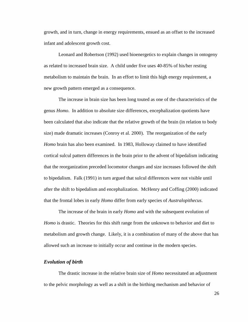
The increase in brain size has been long touted as one of the characteristics of the
genus Homo. In addition to absolute size differences, encephalization quotients have
been calculated that also indicate that the relative growth of the brain (in relation to body
size) made dramatic increases (Conroy et al. 2000). The reorganization of the early
Homo brain has also been examined. In 1983, Holloway claimed to have identified
cortical sulcul pattern differences in the brain prior to the advent of bipedalism indicating
that the reorganization preceded locomotor changes and size increases followed the shift
to bipedalism. Falk (1991) in turn argued that sulcul differences were not visible until
after the shift to bipedalism and encephalization. McHenry and Coffing (2000) indicated
that the frontal lobes in early Homo differ from early species of Australopithecus.
The increase of the brain in early Homo and with the subsequent evolution of
Homo is drastic. Theories for this shift range from the unknown to behavior and diet to
metabolism and growth change. Likely, it is a combination of many of the above that has
allowed such an increase to initially occur and continue in the modern species.
Evolution of birth
The drastic increase in the relative brain size of Homo necessitated an adjustment
to the pelvic morphology as well as a shift in the birthing mechanism and behavior of

27
human ancestors. The functional morphology of the pelvis is a compromise between
locomotion and parturition (Walrath 1997). While the evolution of bipedal locomotion
primarily altered the shape of the pelvis into an efficient walking machine,
encephalization secondarily demanded a reorganization of the bipedal human pelvis for
birth. This compromise resulted in a less efficient locomotor form which differed from
bipedal human ancestors such as the Australopithecines who birthed smaller brained
infants (Abitbol 1987; Lovejoy 1988). In order to remain bipedal and successfully birth
babies with larger crania, the human pelvis had to expand in an anterior-posterior
dimension. This expansion was possible without “compromising either hip
biomechanical or thermoregulatory restraints” (Ruff 1995). The genus Homo could not
become wider from side-to-side (medial to lateral), this would cause the legs to “splay”
and disrupt the equilibrium of the joint (Fischman 1994; Ruff 1995). For females to
birth larger headed infants, both the structure of the birth canal as well as the mode of
birth changed from the ancestral form (Berge et al. 1984; Rosenberg and Trevathan 1995;
Rosenberg 1992; Stewart 1984; Trevathan 1996). These competing pressures created
what is commonly known as the “obstetric dilemma” (Washburn 1960).
Birth in humans is both difficult and complex. Obstetrically, there are three
important planes present in the pelvis: the pelvic inlet, midplane and outlet (see figure 1
and 2 below). The human neonate has to pass through these three apertures during the
birthing process (Greene and Sibley 1986). In humans, each of these openings is widest
in a different dimension, and this results in the modern rotational birthing process. The
pelvic inlet, the most superior opening or the “brim” of the pelvis, has it longest
dimension transversely. The human neonate enters the inlet head first with its longest
28
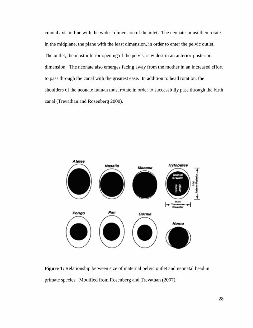
cranial axis in line with the widest dimension of the inlet. The neonates must then rotate
in the midplane, the plane with the least dimension, in order to enter the pelvic outlet.
The outlet, the most inferior opening of the pelvis, is widest in an anterior-posterior
dimension. The neonate also emerges facing away from the mother in an increased effort
to pass through the canal with the greatest ease. In addition to head rotation, the
shoulders of the neonate human must rotate in order to successfully pass through the birth
canal (Trevathan and Rosenberg 2000).
Figure 1: Relationship between size of maternal pelvic outlet and neonatal head in
primate species. Modified from Rosenberg and Trevathan (2007).

29
Figure 2: Birth mechanism for in chimpanzees, Australopithecines and humans.
Modified from Tague and Lovejoy (1986).
30
While human ancestors enjoyed a less strenuous, solitary process in birthing
smaller brained neonates through larger birth canals, birth in Homo sapiens altered social
behavior (Rosenberg and Trevathan 1995; Rosenberg and Travathan 2001; Trevathan
1996). Once rotational birth became a human characteristic, it had been suggested that
natural selection favored assistance for the birthing process to compensate for the bipedal
pelvis, larger brained neonates and neonates emerging facing away from the mother
(Rosenberg and Travathan 2001). Humans are the only species who practice social
births; the twisted birth canal requires a different mechanism, and “obligate midwifery”
increased the survival of the mother and the neonate (Rosenberg and Trevathan 1995).
Natural selection brought about this behavior change (Trevathan 1996).
Along with midwives, the widening of the birth canal is an obvious selective force
for successful parturition (Schultz 1949). While the human birth process continues to be
complex, technological advances have increased the survival of mothers and neonates.
Rather than depending on a sufficiently wide birth canal, many women are able to
survive child birth through cultural adaptation. This may be a factor in the secular
change of the human bony pelvis.
Secular Change
In addition to the evolutionary changes that altered the ancestral pelvic form into
that of the modern human morphology, there continue to be factors that lead to short
term, generational changes. These types of changes are known as secular changes or
secular trends. In the following sections, the secular changes that have occurred in the
31
skeleton over the last four hundred years will be discussed to illustrate how short term
change can alter morphology.
Secular change since the Colonial period: changes over the past 400 years
The change in American skeletal structure over the past 400 years has been
significant. The American environment has provided an arena for unique research; it is
an environment that was novel to the human species. The “melting pot” make-up of
human ancestry and culture as well as the abundance of resources led to a change in the
human constitution. Researchers such as Boas, Angel, Meadows Jantz and Jantz are just
a few of the scholars who have examined how the human skeleton responds to the
American environment. Both Native American populations and those who migrated later
to the Americas have experienced secular change. For the purpose of this dissertation,
secular changes that occur in the bony pelvis within the United States are the focus;
however, in order to grasp how the skeleton can change over a relatively short period of
time, the skeletal changes that have occurred in the United States since the Colonial
Period will be discussed in the following sections.
With the shift from hunting/gathering to agriculture, Native Americans were
suffering from a negative trend when the Europeans “discovered” America (Steckel et al.
2002). This change of diet and mobility as well as endogamy affected both the size and
shape of the skeleton. Steckel and Prince (2001) and Komlos (2003) examined the
equestrian tribes of North America in the nineteenth century. These groups, Crow and
Cheyenne, enjoyed a low population density in relation to their main food source
(Buffalo). This resulted in a nutritional benefit, and they exhibited a tall stature - perhaps

32
the tallest in the world during the 19th
century. During a time when other Native peoples
were turning to agriculture, these tribes were nomadic. While sedentary peoples were
challenged with increased disease due to population density pressure and dependence on
limited regional resources, the equestrian tribes were more successful. This exemplifies
the effect that shifting from hunter/gather to agricultural lifestyles can exhibit in a
population.
In 1983, Jantz and Willey examined the temporal and geographic patterning of
head height among native peoples in the Plains. They found that head height was the
most important indicator of inter-populational difference, and that the lowering of the
cranial vault appeared to be a trend in the Plains. This change in shape was attributed to
gene flow. Owsley joined Jantz in an examination of the Arikara in 1984. This study
researched the secular change in long bone proportions in this native population from
1600-1800s. Earlier sites were characterized by long femora and short tibiae compared to
later sites. The proximal limbs increased faster than the distal limbs, and the lower limbs
outpaced the upper limbs.
Angel (1976) examined changes that occurred in the US since the colonial period
in blacks and whites. His study included pre-colonial US, colonial US, modern US, and
old world skeletal samples. Angel determined that overall health of those in the United
States improved over the last 400 years. There has been an increase in longevity and a
decrease in juvenile death. In addition, Angel (1982) noted changes in the cranial base
height (measurement taken between basion and bregma) and the pelvic inlet that
coincided with nutrition. Each of these skeletal characteristics grows from cartilage as a
child, and this involves growing against gravity. When nutrition is lacking (child suffers
33
from rickets, lack of protein), these growing bones are affected. The cranial base is
flatter and the inlet is reduced in an A-P dimension (Angel 1982). Over this time period,
skull size increased as a result of vault height which is a reflection of improved, increased
cranial base height. There was also a deepening of the true pelvis-another indicator of
improved conditions. The face also became more linearized and an increase in overbites
resulted. Teeth were also affected by changes in diet during this period- this was a
negative secular trend.
Jantz and Meadows Jantz have provided evidence for secular change since the
1800s in Americans. They examined both cranial and postcranial size and shape
differences that have occurred over time (Jantz 1996; Jantz 2001; Jantz and Meadows
Jantz 2000; Meadows Jantz and Jantz 1999). Their results indicate that vault height and
bone length respond in parallel ways to environmental forces. There has been an increase
in vault height over time (also determined by Angel as discussed above), and the vault
has generally become longer and narrower. The length of the crania has been correlated
with stature; increases in cranial length coincide with increases in stature- an indication
of improved conditions. The Meadows Jantz and Jantz studies (1996; 1999) determined
that shape (the size of a bone in relation to the size of other bones) change has been
greater than the size change in long bones. Long bones have increased in length (white
males exhibit positive secular change in each of the six long bones while black females
are the most stable) and allometry. The Jantz corroboration (1999) also determined that
males have a larger secular increase than females, and whites exceed blacks in changes.
Overall, there has been less change in the face over this time period as compared with
changes in the vault.

34
Perhaps the most well known study of the effect of the American environment
was presented by Boas (1911). Boas’ work will be covered in a separate section because
of its ground-breaking importance; however, it is necessary to mention it here in the
discussion of American skeletal changes. Boas claimed that the American environment
could change the head form of children of immigrants. While the above has indicated
that several cranial changes have occurred in Americans over the last 400 years, there is
no claim or indication that these changes are converging into an American types- there is
more of a parallel movement.
While the skeletal changes in blacks and whites largely indicate improved living
conditions and success, this is a simplistic view. Genetics, industrialization, social
inequality and population structure are a few of the factors that can and will continue to
modify these effects. Secular change can be either positive or negative. Since the early
1900’s, changes in most Americans indicate a positive trend; however, as Komlos (2007)
has indicated, there is a cessation of secular change in height in the US. The interaction
between genes and environment continues to change. Humans have the greatest ability of
all animals to control their environment, but there is a limit to this success.
Boas and cranial plasticity
In 1910, Boas teamed up with the Immigration Commission to study the effect of
the American environment on immigrants. He determined that there was a significant
change in the head form of children of immigrants; there was American assimilation.
Boas focused on the two extreme cases of change in his study: Sicilians and Hebrews. In
each of these groups, he found that there was a difference in head type between the

35
immigrant parents and the US born children. Sicilian children had round heads while
their parents were more long-headed; in contrast, Hebrew children were long-headed
compared to their parents. These findings were controversial. Until this point, genetics
were thought to determine the head shape, and essentialist typologies were developed to
differentiate between ancestral groups. Boas’s findings challenged the racialist approach
of the day and called into question the use of cranial morphology in the identification of
peoples by “race”.
While Boas’s finding have been quoted and re-quoted as gospel since the early
1900s, they have also been a serious impediment to the study of craniometrics and
populations. Studies of environmental effects and secular change have indicated that
there are cranial measurements that are effected by nutrition and climate (cranial base,
cranial length); however, there are limits to this effect as well as a lack of convergence
between ancestral groups of people. In terms of understanding the plasticity of the
human head form, the camp is still divided.
Hulse was a student of Earnest Albert Hooten. He examined how immigration
and exogamy affected the morphology of Swiss immigrants. Hulse (1962) found that
population structure influences cranial morphology, an idea which Boas had also
considered as a possible cause of change in the United States. Exogamy coincides
(obviously) with immigration and this makes interpretation based completely on
environmental conditions difficult. Stature and head length were characteristics that were
most obviously affected- an indication of better health and nutrition.
After nearly 100 years of using Boas as the pillar of plasticity, his findings have
been reanalyzed. While Boas claimed that there were drastic differences between

36
immigrant and US born, current research indicates otherwise. Sparks and Jantz (2002)
used Boas’s data and subject them to more vigorous and modern statistical analyses.
They determined that Boas’s claims were not based on statistical significance. Sparks
and Jantz noted that there were shifts in measurements between the groups, and while
most of the measurements were significant, they were not drastic differences. There was
also no indication that the American environment could produce an American type.
Long-headed populations were still long-headed while those groups characterized by
shorter-heads maintained their shortness. When examining the cranial index by age
(breadth/length x100), Jantz also noted that the plasticity observed in Sicilians actually
occurred in Europe. In addition, the pattern of changes that were experienced by the
Hebrews and Sicilians differed. In Sicilians, the CI was altered because of a shortened
cranial length while Hebrew change in both dimensions. As discussed above, Hulse
(1962) indicated that an increase in cranial length corresponds to better nutrition and
health. This indicates that the Sicilians actually experienced a poor environment in the
US in relation to Sicily.
In contrast, Gravlee and colleagues (2003a; 2003b) reanalyzed Boas’s data but
supported his findings. Cranial morphology was significantly changed through
interaction with the American environment. However, while Gravlee and colleagues
noted significant differences, these differences were also less than drastic. While there
were changes in the cranial index, the ethnic differences far outpaced the immigration
differences. Gravlee also failed to support a convergence to an American type.
Where do we stand? In 2003, Armelagos and VanGerven alleged that cranial
index could change by a magnitude of a race in one generation continuing in the tradition
37
of Boas. Many physical anthropologists continue to rail against the use of cranial
morphology to identify ancestral groups of people. However, others have succeeded in
showing that the plasticity of the human head form cannot erase genetic variation.
Klepinger (2001) examined the use of historical stature estimation on current populations.
She found that secular trends in stature (which are paralleled by cranial secular trends)
are overshadowed by non secular populational variation. Relethford (2004) also
determined that the underlying patterns of population structure could not be erased or
obscured by plasticity. He referred to plasticity as “noise” when looking for underlying
differences between groups. There is a neutral model of quantitative variation.
Relethford also briefly comments that Boas claims of plasticity are small in magnitude.
Holloway presented several questions regarding Boas’s findings that coincide with many
problems addressed by Sparks and Jantz (2002). These included Boas’s apparent lack of
usual statistical vigor and apparent support for environmental determinism which was a
departure for Boas.
Racism was and continues to be a challenge for physical anthropology. Boas’s
study indicated that the use of racial typology was inappropriate and that immigrants
could assimilate in the culture and make-up of the United States. While he was known
for his statistical vigor and research design, both were lacking in his study of immigrant
children, and he makes some acknowledgement of this. Boas debunked a myth that was
not a myth, but his effort was for the betterment of those who wanted to belong to the
“melting pot”.
The use of cranial morphology to identify ancestral groups has been supported
through research. While certain dimensions are affected by environment and nutrition,

38
others remain tied to genetics. Convergence to an American type has yet to be supported.
Through populational and temporal studies, effects can be differentiated and the use of
craniometrics can be appropriately used to help identify population characteristics.
Secular change: Europe versus the United States
Many different explanations have been given as causes of positive secular change.
Nutritional improvements (fruits, protein, amount of food), public infrastructure (water,
sewage, health care access), and breakdown of isolates (immigration, assortative mating,
improved travel) have all been suggested as reasons for improvement of health and a
decrease in morbidity and mortality. Malnutrition and disease, which are interrelated
with socioeconomic status and level of health care, also affect the rates of growth and
maturation (Roche 1979).
The United States, Europe, and other first world countries enjoyed surges in
growth, exemplified by stature, over the past 50 years. These secular changes in height in
the US have ceased, while in Europe, they continue to march upward. Historical
differences, populational change and geography, public infrastructure, environmental
effects, dietary and locomotor behavior are offered as possible explanations for the
differences in secular experience between these two regions.
Europe and the United States are both first world regions. Each has gone through
industrialization, enjoy technological advances and have an abundance of resources (or
the ability to get them). Historically, the United States has participated in two World
Wars and many smaller wars while suffering few attacks on US soil. In contrast, Europe
suffered numerous major attacks which affected both infrastructure and population

39
demography. This is one possible reason for continued increases in Europe; while the US
was able to maintain positive growth, Europe is still in the midst of catch-up or recovery
growth.
The geographical areas of the two regions greatly differ. While the US has free
movement between its states, Europe’s movement between countries is more constrained.
This difference affects gene flow. The breakdowns of isolates, exogamy, and
immigration each have a positive effect on secular change. While these are tenets that
define the melting pot of the United States, there is a decrease in their occurrence in the
latter twentieth century. One area of immigration that has increased in the US is that of
“Hispanic” populations. Historically, these groups are smaller in stature. Their inclusion
into the US population has also likely altered the increase.
Komlos and Lauderdale (2007) determined that population density is strongly and
negatively correlated with height. Higher population density leads to lower heights. The
population density in the US exceeds that in Europe. The majority of US citizens live in
cities. Komlos and Lauderdale indicate that the lag in the US behind Europe is largely a
city phenomenon. Individuals living in the suburbs or moderately sized towns actually
have the best mix of benefits with access and availability to medical care with few
negatives.
Public infrastructure is affected by population density as well as by political and
social choice. According to Bock and Sykes (1989), height in the US is a result of
greater growth in the first two years of life. Ghosh and Bandyopadhyay (2005) found
that lower leg length is a sensitive indicator to malnutrition in children as well. These
studies indicate that stature is largely dependent on adequate (or better) prenatal and child

40
care. While Europe has socialized medical and childcare, the US is sadly lacking both.
While there are some social programs in place to benefit the lower socioeconomic groups
in the US, they are often complicated to access.
The continued secular increase in weight in the US is indicative of chronic over-
nutrition. While stature continues to increase in Europe, the US has ceased getting taller
and continues to get wider. Food that is poor in nutritional value is easily attained while
more beneficial fare can be harder and more costly to attain. Hot dogs cost less than pork
chops; chips cost less than peppers, and milk cost twice as much as soda pop. Portion
sizes vary drastically between Europe and the US. In the US, we eat poorly, and we eat
more.
Locomotor trends differ between the two regions, and this affects growth. While
public transportation is available in both regions, its accessibility and use differ. In the
US, cars are king. The cost of fuel favors the US- this is actually a detriment to the
health of the population. Sidewalks are absent in many cities in the US; returning to
Komlos and Lauderdale (2007), this supports the theory that cities are the main areas of
stature lag. Locomotor trends as well as population density and industrialization have all
contributed to increased pollution in the US- especially in the cities. Pollution will also
have an effect on the health and stature of the population (Roche 1979).
The decrease in physical activity has also affected the shape of individuals. While
the US has reduced the amount of physical education in schools (only one state requires
four years of high school physical education- Illinois), children in Sweden have marked
increases in physical fitness between 2000-2006 (Raustorp and Ludvigsson 2007). The
health of children affects the height of adults.
41
Several possible reasons have been given for the cessation of secular increase in
height in America, specifically the United States. Komlos (2003) specifically focused on
population density while Roche (1979) indicated that pollution could reverse secular
change. It is also possible that the US has hit the “genetic ceiling”. While the
environment is able to modify the effects of growth, genetics constrains the response.
This would place the cause in the realm of gene flow. Likely, it is a combination of
environmental and genetic factors.
Factors affecting the growth/formation of the pelvis
Throughout the introduction and the literature review, factors that alter the form
of the human bony pelvis have been briefly mentioned. Because this research is focusing
on changes in the modern pelvic girdle, several of these factors will be highlighted in the
following section because their effects on the growth and formation of the current
morphology are of interest. While these factors are separated into subheadings, it must
be noted that each factor interacts in known and unknown ways with the others. Secular
and evolutionary changes occur because of interactions between innumerable and oft
amorphous factors. It is a challenge to tease out a few of the effects from the mix.
Genetic Factors
Groups of formally isolated peoples funneled through Ellis Island prior to settling
in the United States. Many came from small populations that continually drew from
limited gene pools. Research has shown that upon entering the United States, isolated

42
peoples benefited from an increased genetic stock. Exogamy resulted in greater marriage
distance and genetic outbreeding which led to increased stature (Dubrova et al. 1995)
The size and shape of the pelvis has also been shown to have some genetic component.
Abitbol reported that the gynecoid or “normal” female pelvis was displayed when a
female was not exposed to strenuous adolescent work and acquired erect posture at the
usual age because shape is genetically determined as a result of obstetric demands (1996).
Angel (1976) found that the offspring of exogamous American Swiss and Italian matings
were taller than endogamous offspring; he determined that mixture followed then by
improvements in diet, disease-control and living conditions should all act to increase size.
Skeletal breadth tends to have higher heritability than weight, circumference, and
skinfolds; soft-tissue traits are more easily altered by the changing nutritional
environment of individuals (Cameron 2002). A greater proportion of variance in soft
tissue is explained by environment than in than skeletal tissues which respond less
quickly to changes in nutritional status. The heritability of bi-iliac breadth has been
determined to be between 0.34 (India) and 0.73 (Belgium) (Cameron 2002).
Stature
Most industrialized countries have revealed a trend toward increasing growth and
development in children and greater adult stature in the last 100-150 years (Dubrova et al.
1995). Maternal stature has been positively correlated with pelvic size, and obstetricians
regard maternal stature as “an anthropometric correlate of her reproductive efficiency”
(Tague 2000). Taller women suffer from fewer cephalopelvic complications including
cesarean sections, stillbirths, and perinatal mortality, indicative of a larger pelvic outlet

43
and inlet. However, not all dimensions are uniformly affected by maternal size.
Transverse diameter of the outlet, the posterior space of the inlet, subpubic angle, and
angulation of the sacrum are generally independent of non-pelvic measures of size
suggesting that the selection for obstetric sufficiency is independent of selection for
larger body size (Tague 2000). Western women are generally taller than women in less
developed areas, and this is also exemplified in the ability to birth larger babies vaginally
(Abitbol et al. 1997).
Sex
Men and women have hips that serve different functions. While both sexes
developed bony pelves that enabled them to walk upright, only females required pelvic
outlets that were sufficient to pass a large brained neonate. This fundamental difference
results in the sexually dimorphic characteristics that are manifest in the human os coxa
and sacra. Female os coxae are more shallow, broader, and less acutely flared with a
rectangular pubis and longer ischiopubic ramus (Shipman et al. 1985). The inferior pubic
ramus of females is concave with a subpubic angle that is usually greater than 90 degrees.
Males exhibit a more triangular pubis, convex inferior pubic ramus, and a subpubic angle
of approximately 60 degrees (Shipman et al. 1985). The acetabulum is smaller and
shallower in females while the auricular surface is more raised. Females usually have a
wider sciatic notch that may approach 90 degrees.
The difference in structure is largely attributed to the need for females to bear
large headed babies; a broad pelvis with large pelvic inlet and outlet is necessary for
birthing (Shipman et al. 1985). However, in order to be efficient bipedally, a narrow

44
pelvis that places hip joints closer together minimizes the side-to-side displacement of the
body during walking and maximizes mechanical efficiency. Thus, there needs to be a
compromise; human infants are less mature at birth and the female pelvic structure is less
bipedally efficient (Shipman et al. 1985).
Ancestry
While stature and sex may add obvious variation to the human pelvic form,
ancestry also plays a role in the shape of the pelvis. Differences in musculature between
blacks and whites have been shown to alter the formation of bone in individuals. Both
size and shape differ in the os coxa between blacks and whites (Synstelien 2001). There
is a greater distance in white individuals between the anterior superior and inferior iliac
spines, the anterior superior spine and point ilioauricular, a greater depth of the iliac fossa
and lesser depth of the notch between the anterior superior and inferior iliac spines when
compared to blacks. Synstelien (2001) also found that there was a significant mean
increase in white males for 14 of 19 variables measured over blacks.
Environmental Factors
Altitude and climate also affect the final form of the adult human pelvis. Two
well known and often cited “rules” regarding ecological effects on the skeleton are
credited to Bergmann (1847) and Allen (1877). Bergmann's rule states that "races of
warm blooded vertebrates from cooler climates tend to be larger than races of the same
species from warmer climates" (Mayr 1956) while Allen’s rule focuses on limb lengths

45
and extremity proportions. In 2002, Ruff determined that the dimorphism present in
modern humans exists as a gradation along latitudinal climates. Geography and climate
altered the shape and size of the human form; however, Ruff warned that a genetic
component also exists.
Katzmarzyk and Leonard (1998) corroborated the findings of Bergmann, Allen,
and Ruff. They also found that secular trends in body size do not appear to be equal
across populations of different climatic zones; there is an increase in body mass that
appears to be disproportionately larger in tropical regions. The impact of acculturation
and lifestyle change and the associated improvements in health care and nutrition
disproportionally affect developing world pops of the tropics and subtropics (Katzmarzyk
and Leonard 1998). Genetics as well as nutrition were found to have moderated the
influence of climatic factors (Katzmarzyk and Leonard 1998).
Nutritional Factors
The shape of the pelvis has been shown to be effected by fetal and childhood
nutrition. Nicholson (1945) found that a period of malnutrition, like the war of 1914-
1918, may have led to the low length of the conjugate diameter in England. In contrast,
rural populations in England escaped the effects of malnutrition of war and exhibited a
half inch higher diameter. This may have occurred because of malnutrition during early
years of weight bearing. Nicholson also found a correlation between the length of
conjugate diameter and stature with a one centimeter above average diameter
corresponding to a stature that is seven centimeters taller than average. Angel (1976)
determined that the pelvic inlet responds to levels of childhood suboptimal nutrition

46
caused by war or lower socioeconomic class with a reduced AP diameter and pelvic
index; he found significant changes from the colonial to modern pelvic index. Rickets
also alters the obstetric success of females by decreasing the inlet AP diameter;
nutritional deficiencies distort growth at cartilage joints inhibiting bone formation such as
the AP arch of pelvis (Angel 1982; Kaltreider 1951). According to Weyl (1977), diet
(especially meat consumption), a shortage of food, climatic change, and dysentery will all
effect the pelvic inlet.
Mothers born and raised in third world countries are, on average, shorter, have
less weight, have narrower pelvic dimensions, and give birth to smaller babies than
women born in United States (Abitbol et al. 1997). This could be due to a low-protein
diet and inadequate prenatal care. Mothers born outside of the United States but who eat
a high-protein diet and have adequate health care after migrating to the United States as
adults give birth to relatively large newborns (Abitbol et al. 1997). Marked
cephalopelvic disproportion and severe dystocia which frequently leads to cesarean
section births occurs in these migrant women (Abitbol et al. 1997). Good nutrition
during infancy, childhood, and adolescence will contribute to high stature in adulthood
with adequate pelvic dimensions for women, and nutrition with an emphasis on more
protein can increase fetal weight by 25% while minimum to moderate prenatal care
(high-protein diet, iron, calcium, vitamins) can see fetal weight increase up to 50% as
compared to no care (Abitbol et al. 1997).
Activity Factors
Becoming bipedal ultimately set about the evolution of the hominid pelvis.
Walking upright required an alteration in the form of the os coxae and the sacrum.

47
Walking continues to alter the form of the pelvis. Children, specifically females, who
walk at an earlier age have been shown to have a different pelvic shape that those who
walk after 14 months of age (Abitbol 1996). Early walkers exhibit a platypelloid shape
which is transversely wide and narrow anteroposteriorly. In contrast, later walkers
develop a form that is narrow transversely and wide anteroposteriorly, a shape referred to
as anthropoid. Strenuous activity prior to adulthood has also been shown to effect the
adult shape of the pelvis leading to a more triangular pelvic inlet or android shape
(Abitbol 1996). Additionally, early pregnancy will distort the primary shape of the
female pelvis (Abitbol 1987).
Other Factors
In addition to the factors discussed above, technology and culture need to be
explored whenever humans are studied. Culture often dictates the activity performed by
males and females. Divisions of labor between males and females has been linked to
difference in the pelvic form (Ruff 1987). Pelvic dimorphism is accentuated when
cultures allow different activities, and dimorphism is often less accentuated when there
was little or no gender differentiation in terms of physical activity (Abitbol 1996).
Increases in body size, shape, rates of maturation, and changes in body compositions of
children are also associated with changes in child-labor practices, family size, household
size (Roche 1979).
Technological advances are also adding to the factors that can alter the form of
the human bony pelvis. As discussed earlier, between 1996 and 2005, Cesarean section
procedures increased 46% to make up 30.2% of all births in the United States. Its effect

48
on the shape and size of the pelvic canal is not completely known. In Germany,
technology has been linked to a decrease in the female dimensions of the birth canal over
the last 80 years (Lehmann et al. 1992; Wischnik et al. 1992).

49
Chapter 3
Hypotheses and Samples
Having covered the background necessary to understand the growth and
development of the modern human pelvis, this chapter will outline the hypotheses driving
this research and the samples used in this study.
Ultimately, this is a project focusing on secular change. As such, differences that
occur over a relatively short time will be examined. Changes in the dimensions of the
pelvic planes in addition to the height and breadth of the pelvis are of primary
importance. Size and shape differences are both of interest.
Hypotheses
Improvements in nutrition and general health have been shown to lead to
increased stature and physical size. To determine if the same trends are altering the
pelvic girdle, overall size changes in inter-landmark distances will be examined. In
addition, the femoral head of each individual will be measured to test for changes in body
size (Delprete 2006; McHenry 1986). The mean femoral head diameter will be used, if
necessary, to remove size as a primary difference and to focus on shape. While size will
be examined, if left un-controlled, shape differences could be missed.
50
Body & Pelvis Size
Increases in stature and overall body size have been shown to occur over time in
this study sample. As discussed in the literature review, individuals in the United States
have benefited from improved conditions, and until very recently, as a group, they have
experienced unprecedented increases in stature. A coinciding increase in the mean
femoral head diameter is expected to occur in each of the ancestral groups dependent on
birth cohort. In concert, os coxa height and breadth, and overall pelvic breadth are also
expected to increase due to improved nutrition and environment. Additionally, analyses
using 3D morphometrics produce centroid sizes for each individual that will enable
overall pelvic size to be compared across cohorts, and these results that will be examined
in addition to those found using traditional metrics.
Pelvic canal shape
With improved nutrition, the pelvic inlet should mirror the secular change in
stature. An increase in the anteroposterior dimension of the inlet through time is
expected to occur within the samples measured. Additionally, as nutrition has improved,
activity has decreased. With this decrease in activity, specifically strenuous activity of
children, the number of individuals with android shaped pelvic inlet (triangular) is
expected to decrease. Principal component scores produced through the rotation,
translation, and scaling of Procrustes Analyses will illuminate changes occurring in shape
between the cohorts.

51
Lehmann, Wischnik, and colleagues found that the female pelvis in Germany has
become less favorable for birthing and more bipedally efficient over the last 80 years
(Lehmann et al. 1992; Wischnik et al. 1992). Increased use of technology, such as
cesarean intervention, may also be altering the shape of the pelvic canal. If this is the
case, there should also be a decrease in the sexual dimorphism among the samples. There
should be a shift by females to a more masculine, bipedally more efficient, form.
Samples
Three skeletal collections were used in this study. The Hamann-Todd Human
Osteological Collection housed at the Cleveland Museum of Natural History in
Cleveland, Ohio, the Robert J. Terry Anatomical Skeletal Collection curated at the
Smithsonian National Museum of Natural History, and the William M. Bass Donated
Skeletal Collection maintained by the Anthropology Department of the University of
Tennessee, Knoxville. These collections were chosen for a variety of reasons. First and
foremost, these invaluable skeletons represent individuals living in the United States
between 1822 and the present. The United States is a unique combination of novel
environment and melting pot. Since each of the individuals used in this study died in the
US, each was subjected to the conditions that coincide with living in this environment.
This is not to say that each group was exposed to identical environments. Each collection
represents different facets found within the country, and those differences will be
highlighted and tested for to determine which factors result in shifts in morphology
between the samples.
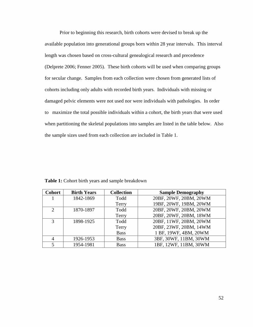
52
Prior to beginning this research, birth cohorts were devised to break up the
available population into generational groups born within 28 year intervals. This interval
length was chosen based on cross-cultural genealogical research and precedence
(Delprete 2006; Fenner 2005). These birth cohorts will be used when comparing groups
for secular change. Samples from each collection were chosen from generated lists of
cohorts including only adults with recorded birth years. Individuals with missing or
damaged pelvic elements were not used nor were individuals with pathologies. In order
to maximize the total possible individuals within a cohort, the birth years that were used
when partitioning the skeletal populations into samples are listed in the table below. Also
the sample sizes used from each collection are included in Table 1.
Table 1: Cohort birth years and sample breakdown
Cohort Birth Years Collection Sample Demography
1 1842-1869 Todd
Terry
20BF, 20WF, 20BM, 20WM
19BF, 20WF, 19BM, 20WM
2 1870-1897 Todd
Terry
20BF, 20WF, 20BM, 20WM
20BF, 20WF, 20BM, 18WM
3 1898-1925 Todd
Terry
Bass
20BF, 11WF, 20BM, 20WM
20BF, 23WF, 20BM, 14WM
1 BF, 19WF, 4BM, 20WM
4 1926-1953 Bass 3BF, 30WF, 11BM, 30WM
5 1954-1981 Bass 1BF, 12WF, 11BM, 30WM
53
Hamann-Todd
The Hamann-Todd Human Osteological Collection is currently the largest
collection of modern human skeleton with documentation that exists in the world. This
collection was started by Carl A. Hamann while professor of anatomy at the medical
school at Western Reserve University in Cleveland, Ohio, from 1893-1912. Skeletons
were collected from cadavers after dissection. In 1912, Hamann became dean of the
medical school and supported incoming anatomy professor Thomas Wingate Todd in
enlarging the collection until Todd’s death in 1938. In 1968, over 3000 human skeleton
were moved to the Cleveland Museum of Natural History where they are currently. This
collection is composed of individuals born between 1835 and 1913, age 0 to 105 with
many coming from a lower socioeconomic background. For this study, adult males and
females of black and white ancestry were used.
In an effort to collect an evenly distributed sample, the goal was to digitize and
measure 20 individuals per birth cohort per ancestry (black and white) and sex. In the
Hamann-Todd collection, this protocol was attainable except for white females in the
more recent birth cohort (1898-1925). In the collection, there were only 11 skeletons that
fit the research criteria.
Terry
Robert J. Terry began collecting skeletons for research in 1898; however, his
early efforts were riddled with element loss and commingling. During his tenure at
Washington University Medical School in St. Louis, Missouri, from 1921 to 1946, Terry
amassed the majority of the specimen current housed in the Smithsonian National
54
Museum of Natural History in Washington DC. Mildred Trotter, Terry’s successor at
Washington University, added to the collection and is responsible for evening out the
demographic distribution of the skeletal population. Trotter aimed to add younger
individuals, especially white females, to the anatomical collection, and she continued this
work until her retirement in 1964. The collection was donated to the Smithsonian
Institution in 1967.
The Robert J. Terry Anatomical Skeletal Collection has 1728 individual in the
collection with documented demography (Hunt and Albanese 2005). Prior to the Willed
Body Law of Missouri in 1955-56, the majority of cadavers used in dissection were
predominantly unclaimed bodies or individuals who were signed over by family
members. After the passage of the law, signed releases were required prior to use. This
shift in protocol changed the socioeconomic make up of the collection; those collected
prior to 1955 had lower incomes and many died during the depression while those after
1955 were largely from the middle to upper socioeconomic class.
Again, as with the Hamann-Todd collection, an effort was made to collect an
evenly distributed sample of the Terry Collection and to digitize and measure 20
individuals per birth cohort per ancestry (black and white) and sex. In the Terry
collection, the limiting group was the white males born between 1898 and 1925; only 14
skeletons fit the criteria. However, there were additional white females in this birth
cohort, and three additional specimens were measured in an effort to compensate for the
lack in the Hamann-Todd sample.

55
Bass
The William M. Bass Donated Skeletal Collection housed in the Anthropology
Department of the University of Tennessee, Knoxville, is the only one out of these three
collections still growing. Rather than being made up of dissected cadaveric donations,
the Bass collection is made up of skeletons collected from donated bodies that have
decomposed at the William M. Bass Anthropological Research Facility. Over 60% of
those in the collection were donated by family members. Most of the remaining 40%
come from self (pre) donors or medical examiner (unclaimed) donors.
Bass started the collection in 1981 while a professor at the university, and at the
time of sample measurement, there were 750 skeletons. Twenty-three states and two
countries are represented by skeletons in the collection with ages ranging from 0 to 101.
The majority of the collection is made up of white males, and while the demography of
this collection is certainly skewed, the utility of the Bass Donated Collection is high.
This collection is the largest collection of documented skeletal material from people born
during the modern industrial era. As discussed previously, the environment of the United
States has changed drastically over the last century and having research materials that
represent the population currently inhabiting the country is essential to understanding the
current state of the modern skeleton in addition to illuminating incidence of secular
change.
While the sampling protocol of 20 individuals per birth year cohort was the
benchmark for the Bass Donated Collection, this approach was altered. For cohort 3 that
was to overlap with the Terry and Todd collections (1898-1925), the measurement
sample goal was, again, 20 individuals. This was only possible for the white males and

56
females; there, currently, are not that many black individuals born within this time period
contained in the collection. In the Bass Collection, black males and females are
underrepresented. As many individuals that fit the testing criteria were measured in these
cases. For cohort 4 and cohort 5, the sample size goal was increased to 30 since the Bass
Collection was the sole contributor in these birth cohorts. However, again, sample
availability became an issue. In addition to the black males and females, white females
in the most recent birth cohort (1954-1981) were limited.

57
Chapter 4
Measurements and Methods
This chapter will cover the measurements chosen for collection, the method used
for data collection, and the statistical approaches used in the data analysis. To determine
the pertinent measurements that should be taken to determine secular changes in the
human pelvis, an understanding of the organization of the pelvis is essential, and the
regions of the pelvis as well as the historic definitions of pelvic shapes present in humans
will be introduced below. Additionally, measurements were chosen in order to be
comparable to previous studies, and those measurements will also be discussed in this
chapter.
For measurement collection, digitizing was chosen for a number of reasons.
Digitizing the pelvis enabled a large number of data points to be collected in a relatively
short time, and it reduced the need to record a point multiple times. Also, the points are
automatically stored in the computer which removes translation error. The specific
technique used to digitize the pelvic girdle will be outlined following the discussion of
data point selection.
Measurements
Pelvic regions
The pelvic girdle is made up of two regions: the greater (false) pelvis and the
lesser (true) pelvis. The pelvic inlet, or the brim, divides these two regions. The false

58
pelvis, which is the anatomically superior region, houses the abdominal viscera and is
bound by the abdominal wall anteriorly, the iliac fossa laterally, and the fifth lumbar
vertebra ventrally (Scheuer and Black 2000). The brim that separates the regions is
formed by the promontory and alae of the sacrum posteriorly, the iliopectineal lines
laterally, and the pubic crest and symphysis anteriorly. The true pelvis, the inferior
pelvic region, protects the urinary bladder, the rectum, and internal genitalia. The
posterior wall of the true pelvis is formed by the sacrum and the coccyx. Anteriorly, a
shorter wall is formed by the pubic symphysis and the body of the pubis. The lateral
walls of the true pelvis is made up of the inner aspect of the os coxae, the obturator
fascia, and the muscles that cover the obturator foramen (Scheuer and Black 2000).
The most posterior opening of the pelvis is the pelvic outlet. This space, which is
diamond shaped, is bound by the coccyx, ischial tuberosities, and the sacrotuberous
ligaments laterally, and the pubic symphysis anteriorly (Scheuer and Black 2000).
Obstetrically, this posterior opening and the pelvic inlet, which divides the pelvic regions,
are most important. Their shape and size alter efficacy of locomotion and birthing. The
inlet and outlet as well as the pelvic midplane will be the main areas of measurement
concentration in the current study.
Historical pelvic shapes
The shape of the pelvis and the pelvic canal has been of interest for millennia.
Females have a more shallow, broader, and less acutely flared shape with a deeper and
longer ischiopubic ramus (Shipman et al. 1985). The pubis is more rectangular in
females while the pubis is triangular in males. Males also have a more convex inferior

59
pubic ramus and small subpubic angle while females exhibit greater sciatic notches and
larger subpubic angles – each of these characteristics contributed to the more rounded,
open canal found in females (Shipman et al. 1985). Prior to the current modern era,
birthing success was dependent upon the ability for the mother to pass an infant through
the birth canal, and the dimorphic differences were evolutionarily necessary. Generally,
there are four classifications used to describe pelvic canal shape. The names of these four
types vary, but the characteristics are consistent. For purposes here, the terminology will
include the following four types: anthropoid, android, gynecoid, and, platypelloid
(Caldwell and Moloy 1938; Greulich and Thoms 1938; Shipman et al. 1985).
Classification is based on the difference between the anteroposterior diameter and the
transverse diameter of the pelvic inlet. Turner (1885) developed the pelvic index to
quantify canal shape. The Turner Index or Pelvic Index is the anteroposterior diameter of
the inlet times 100 then divided by the maximum transverse diameter. According to the
Turner classification, pelves with an index greater than 95 are designated as dolichopellic
(anthropoid); those with an index of from 90 to 94.9 are mesatipellic (gynecoid); and
those whose index is less than 90 are platypellic (platypelloid) (Turner 1885). Turner did
not define a range for the android pelvis.
An anthropoid pelvis has an oval inlet with its long axis in the A-P dimension and
a narrower transverse diameter. This shape resembles the inlet shape of higher, non-
human primates. Human males are more often anthropoid. Android inlets are small and
heart shaped. The ischial spines are prominent and the pelvic arch is narrow in android
pelves; the inlet is wider posteriorly than anteriorly; it more common in males. The most
common shape is the gynecoid inlet. This shape is rounded and found in approximately
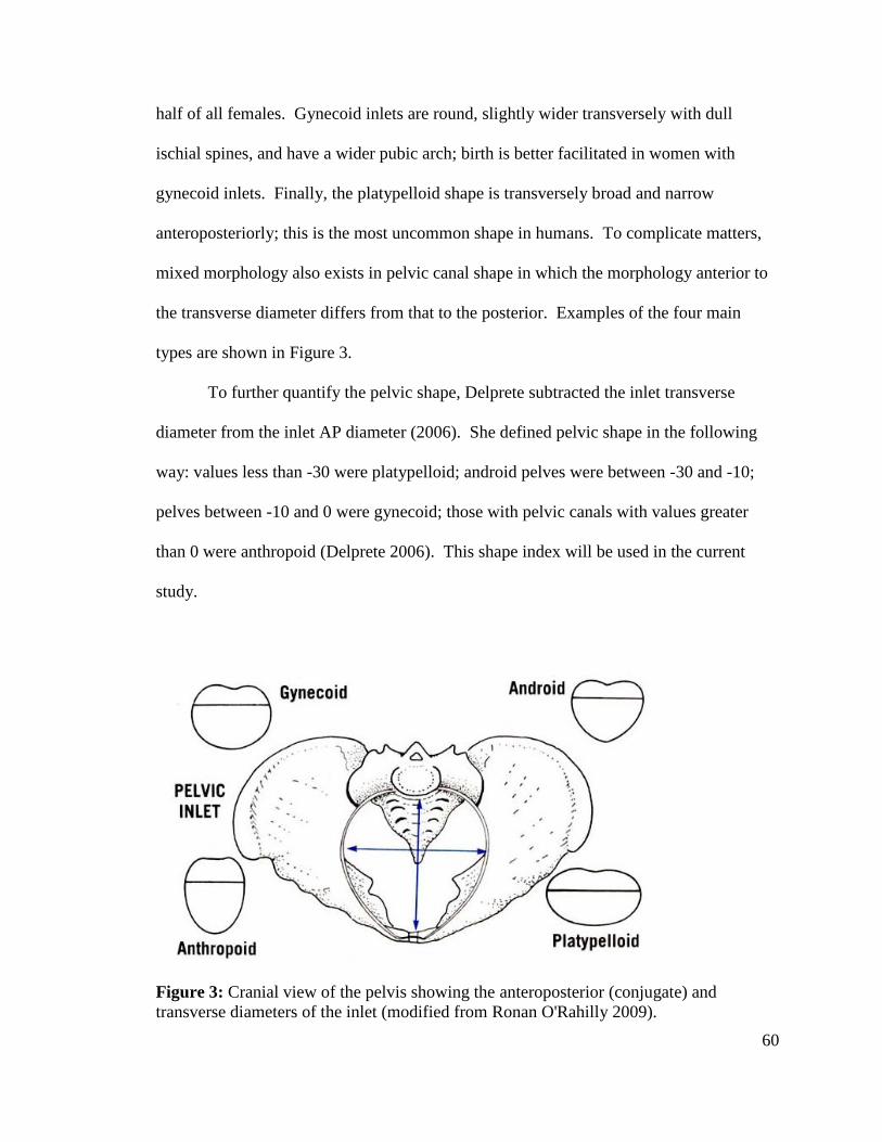
60
half of all females. Gynecoid inlets are round, slightly wider transversely with dull
ischial spines, and have a wider pubic arch; birth is better facilitated in women with
gynecoid inlets. Finally, the platypelloid shape is transversely broad and narrow
anteroposteriorly; this is the most uncommon shape in humans. To complicate matters,
mixed morphology also exists in pelvic canal shape in which the morphology anterior to
the transverse diameter differs from that to the posterior. Examples of the four main
types are shown in Figure 3.
To further quantify the pelvic shape, Delprete subtracted the inlet transverse
diameter from the inlet AP diameter (2006). She defined pelvic shape in the following
way: values less than -30 were platypelloid; android pelves were between -30 and -10;
pelves between -10 and 0 were gynecoid; those with pelvic canals with values greater
than 0 were anthropoid (Delprete 2006). This shape index will be used in the current
study.
Figure 3: Cranial view of the pelvis showing the anteroposterior (conjugate) and
transverse diameters of the inlet (modified from Ronan O'Rahilly 2009).

61
Measurement Selection
After taking into account the hypotheses driving this research, traditional
measurements taken on the pelvis, previous research, and determining the number of
points necessary to visualize the pelvis once plotted in the morphometrics software, 64
pertinent distances were chosen; see Table 1 for a list of measurements. In order to
calculate each of these measurements, 115 points and four arcs were taken from each
articulated pelvis; these points encompass the pelvic canal and all three planes, iliac flare,
sacral curvature, os coxa heights and widths, angles, acetabulum, and obturator foramen;
see Table 2. There are many, many more measurements taken than will be used in the
present study; however, because of the ease of collection using the digitizer, additional
points of interest could be recorded without adding significant time. Also, in order to
create a recognizable 3D image, numerous points were needed. Those measurements not
used here will be utilized in later studies that will build on the results of the present
research.
When choosing skeletal landmarks for measurement, Zelditch and colleagues
(2004) outline five criteria for choosing ideal landmarks; these require the landmark to be
“homologous anatomical loci that do not alter their topological position relative to other
landmarks, provide adequate coverage of the morphology, can be found repeatedly and
reliably, and lie within the same plane.” Each of these criteria was taken into account
when choosing the landmarks used in this research. The fifth criteria, for points to be
most readily and reliable located, presented the greatest challenge when working with the
pelvic girdle. According to Bookstein, landmarks can be classified into three groups:
Type 1, Type 2, and Type 3 (Bookstein 1991). Type 1 points are those that occur at the

62
intersection of three bones along where sutures come together. These types of points are
easily located and there is relatively low inter- and intra- observer error. While Type 1
landmarks are ideal for reproducibility, unfortunately, the adult pelvic girdle lacks sutures
and Type 1 landmarks. All landmarks used in this study are Type 2 landmarks. Type 2
landmarks are located at tips or ends of bony processes or are points that are the
maximum or minimum points along curvatures; they are defined by local properties of
the bone. While Type 2 landmarks can be problematic, they are more reliable than those
points defined by Bookstein as Type 3 and the only option in the pelvis. Type 3
landmarks are extremal points that are defined by their distance away from another
structure; these types of landmarks can also be defined as constructed landmarks such as
a centroid.
Finally, the measurements and their associated landmarks can be found in Table 2
and illustrated in Figures 4a and 4b. For this study, the following measurements were
examined to test the hypotheses: AP diameter of the inlet, midplane, and outlet;
transverse diameter of the inlet, midplane, and outlet; the height and breadth of the left
and right os coxa; the sacral breadth; internal and external breadth of the pelvic girdle;
the femoral head diameter. These measurements are in bold in Table 2 and shown in the
wireframe in Figure 4b. In addition, two measurements were calculated for this study.
Turner’s Index and Pelvic Inlet Shape utilized the inlet AP and transverse diameters.
Turner’s Pelvic Index is inlet AP diameter times 100 and then divided by the inlet
transverse diameter. Pelvic Inlet Shape was calculated by subtracting the transverse
diameter from the AP diameter. The range values for each pelvic type were defined
above.
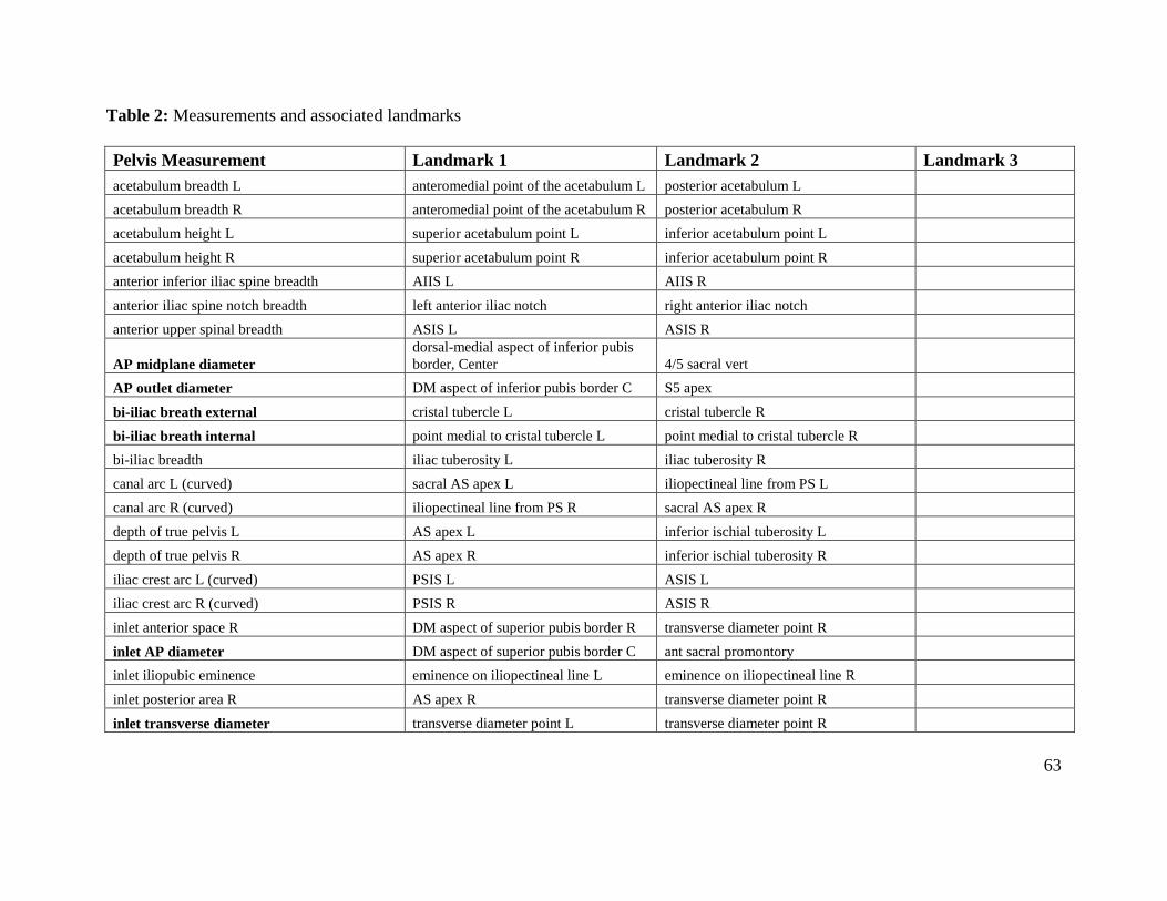
Table 2: Measurements and associated landmarks
63
Pelvis Measurement Landmark 1 Landmark 2 Landmark 3
acetabulum breadth L anteromedial point of the acetabulum L posterior acetabulum L
acetabulum breadth R anteromedial point of the acetabulum R posterior acetabulum R
acetabulum height L superior acetabulum point L inferior acetabulum point L
acetabulum height R superior acetabulum point R inferior acetabulum point R
anterior inferior iliac spine breadth AIIS L AIIS R
anterior iliac spine notch breadth left anterior iliac notch right anterior iliac notch
anterior upper spinal breadth ASIS L ASIS R
AP midplane diameter
dorsal-medial aspect of inferior pubis
border, Center 4/5 sacral vert
AP outlet diameter DM aspect of inferior pubis border C S5 apex
bi-iliac breath external cristal tubercle L cristal tubercle R
bi-iliac breath internal point medial to cristal tubercle L point medial to cristal tubercle R
bi-iliac breadth iliac tuberosity L iliac tuberosity R
canal arc L (curved) sacral AS apex L iliopectineal line from PS L
canal arc R (curved) iliopectineal line from PS R sacral AS apex R
depth of true pelvis L AS apex L inferior ischial tuberosity L
depth of true pelvis R AS apex R inferior ischial tuberosity R
iliac crest arc L (curved) PSIS L ASIS L
iliac crest arc R (curved) PSIS R ASIS R
inlet anterior space R DM aspect of superior pubis border R transverse diameter point R
inlet AP diameter DM aspect of superior pubis border C ant sacral promontory
inlet iliopubic eminence eminence on iliopectineal line L eminence on iliopectineal line R
inlet posterior area R AS apex R transverse diameter point R
inlet transverse diameter transverse diameter point L transverse diameter point R
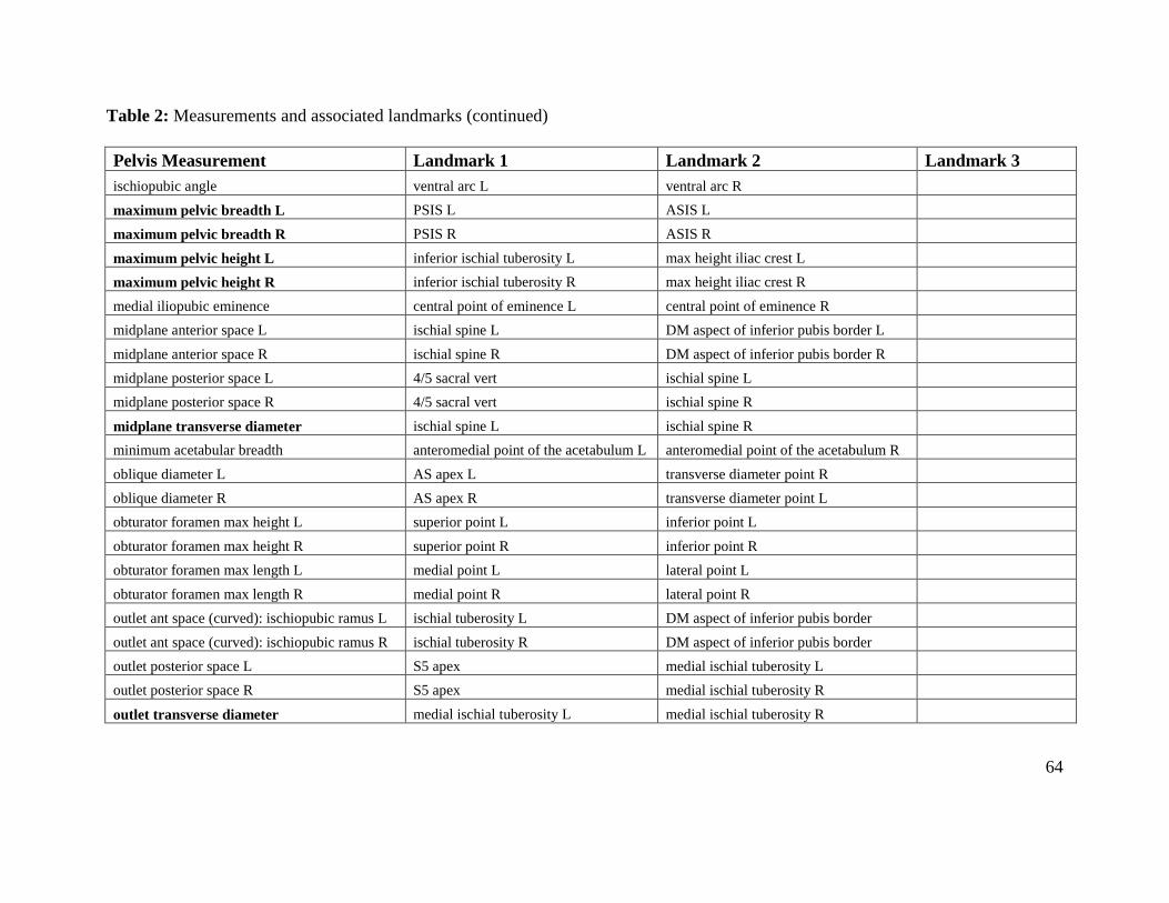
Table 2: Measurements and associated landmarks (continued)
64
Pelvis Measurement Landmark 1 Landmark 2 Landmark 3
ischiopubic angle ventral arc L ventral arc R
maximum pelvic breadth L PSIS L ASIS L
maximum pelvic breadth R PSIS R ASIS R
maximum pelvic height L inferior ischial tuberosity L max height iliac crest L
maximum pelvic height R inferior ischial tuberosity R max height iliac crest R
medial iliopubic eminence central point of eminence L central point of eminence R
midplane anterior space L ischial spine L DM aspect of inferior pubis border L
midplane anterior space R ischial spine R DM aspect of inferior pubis border R
midplane posterior space L 4/5 sacral vert ischial spine L
midplane posterior space R 4/5 sacral vert ischial spine R
midplane transverse diameter ischial spine L ischial spine R
minimum acetabular breadth anteromedial point of the acetabulum L anteromedial point of the acetabulum R
oblique diameter L AS apex L transverse diameter point R
oblique diameter R AS apex R transverse diameter point L
obturator foramen max height L superior point L inferior point L
obturator foramen max height R superior point R inferior point R
obturator foramen max length L medial point L lateral point L
obturator foramen max length R medial point R lateral point R
outlet ant space (curved): ischiopubic ramus L ischial tuberosity L DM aspect of inferior pubis border
outlet ant space (curved): ischiopubic ramus R ischial tuberosity R DM aspect of inferior pubis border
outlet posterior space L S5 apex medial ischial tuberosity L
outlet posterior space R S5 apex medial ischial tuberosity R
outlet transverse diameter medial ischial tuberosity L medial ischial tuberosity R
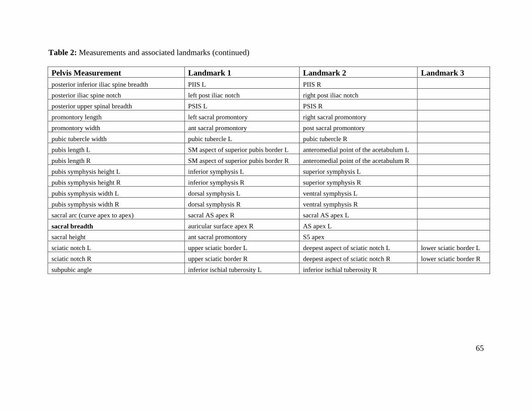
Table 2: Measurements and associated landmarks (continued)
65
Pelvis Measurement Landmark 1 Landmark 2 Landmark 3
posterior inferior iliac spine breadth PIIS L PIIS R
posterior iliac spine notch left post iliac notch right post iliac notch
posterior upper spinal breadth PSIS L PSIS R
promontory length left sacral promontory right sacral promontory
promontory width ant sacral promontory post sacral promontory
pubic tubercle width pubic tubercle L pubic tubercle R
pubis length L SM aspect of superior pubis border L anteromedial point of the acetabulum L
pubis length R SM aspect of superior pubis border R anteromedial point of the acetabulum R
pubis symphysis height L inferior symphysis L superior symphysis L
pubis symphysis height R inferior symphysis R superior symphysis R
pubis symphysis width L dorsal symphysis L ventral symphysis L
pubis symphysis width R dorsal symphysis R ventral symphysis R
sacral arc (curve apex to apex) sacral AS apex R sacral AS apex L
sacral breadth auricular surface apex R AS apex L
sacral height ant sacral promontory S5 apex
sciatic notch L upper sciatic border L deepest aspect of sciatic notch L lower sciatic border L
sciatic notch R upper sciatic border R deepest aspect of sciatic notch R lower sciatic border R
subpubic angle inferior ischial tuberosity L inferior ischial tuberosity R

66
Figure 4a: Illustration of landmarks

67
Figure 4b: Wireframe illustration of landmarks used in this research. Landmark identifications of the numbered points can be found
in Table A13 in the appendix.

68
Methods
For each specimen, the pelvic girdle was rearticulated and the maximum femoral
head diameter was measured. The left femoral head was measured to the nearest tenth of
a millimeter using Mitutoyo digital calipers unless damaged; in cases of damage or
missing left femora, the right femur was measured. An input tool was attached to the
calipers and measurements were saved directly into an Excel spreadsheet which
eliminated the chance of recorder error. The os coxae and the sacra were examined for
damage and areas of fusion. Damage in landmark areas and sacra with fused coccygeal
or lumbar vertebra were excluded from the sample.
Once the three bones were pulled for measurement, the maximum height and
breadth of each os coxa was located using an osteometric board and marked with chalk.
Additionally, once the bones were rearticulated, the maximum pelvic breadth was
measured and marked. After articulation and marking, the pelvic girdle was mounted on
clay pillars in preparation for digitizing with care to ensure each landmark was in reach
of the arm of the 3DX microscribe digitizer. If any shifting occurred in the rearticulated
girdle or of the pillars, the setup was redone.
Articulating the pelvic girdle
Prior to data collection, the three skeletal elements of the pelvic girdle needed to
be rearticulated. Rubber bands of various sizes were used in this process. In order for
the structure to remain stable during data collection, three to five bands were used. The
technique used to rearticulate the girdle was modeled after those used by Tague in his
numerous works on the pelvis, Ruff, Hager, and Delprete (Delprete 2006; Hager 1989;

69
Ruff 1995; Tague 1989; 1992; 1995; 2000; 2007). No compensation was made during
the rearticulation for the symphyseal disc or other soft tissue that is present in living
humans. This is consistent with previous studies and makes the measurements
comparable to past research; it also reduces the error introduced through estimating the
thickness of soft tissue.
Digitizing the pelvic girdle
After determining which measurements would be collected, the landmarks used in
calculating these distances were listed. It became apparent that many of the
measurements utilized the same or similar landmarks. In an effort to decrease
remeasurement error, a 3DX microscribe digitizer was used to collect the data points.
Using the digitizer required taking a point’s coordinates a single time; distances could
then be calculated using a single recorded point rather than determining a landmark’s
position multiple times. The digitizer also allowed for the collection and recording of
many points in one session. When digitizing crania, 3Skull, a paradox based program
written by Steve Ousley (2004), is the software used to collect the coordinates and
calculate the inter-landmark distances. For this project, 3Skull was adapted to collect and
calculate those landmarks of interest. In all, 115 points and four arcs were collected from
each pelvic girdle.

70
Statistical Analyses
Once all of the pelvic girdles were digitized and the femoral heads were
measured, the inter-landmark distances and femoral head measurements were imported
into NCSS statistical software for analysis (Hintze 2006). The tests run and results of
each statistical test will be discussed in a following section. In addition to analyzing the
traditional metrics, the coordinates of each landmark were input into the 3D
morphometric software freeware Morphologika2 (O'Higgins and Jones 2006) and
MorphoJ (Klingenberg 2008). The process through which the geometric morphometric
analyses proceeded will also be discussed below.
Initial Testing
Prior to running any statistical analyses focusing on secular change, it was
necessary to determine whether similar cohorts could be pooled by sex, ancestry, and/or
collection. Multivariate analyses of variance (MANOVA) were run to determine whether
inter-landmark distances differed between groups based on ancestry and/or sex.
After separating the data into single sex and ancestry birth cohorts (1WF for white
females in cohort one, 1BF for black females in cohort one, etc.), the groups were further
separated by collection. The normality of each measurement was tested using
D’Agostino Omnibus Normality test for skewness and kurtosis. When data was normal,
t-tests were used to determine whether there were differences in mean of each
measurement between similar cohorts of differing collections; for example, comparing
the bi-iliac breadth of the 1WFs in the Hamann-Todd Collection to the 1WFs the Terry

71
Collection. When data was not normally distributed, the non-parametric versions of the
t- test, the Wilcoxon Rank-Sum/ Mann-Whitney test, was used.
For comparisons of cohort three, which is made up of individuals from all three
skeletal collections, univariate analysis of variance (ANOVA) was used to test for
differences between the three collections. ANOVA tests were used to determine whether
there were differences when data was normal; when data was not normally distributed,
the non-parametric test, and the Kruskal Wallis test was used. T-test were run on each on
pair (Terry-Todd, Bass-Terry, Bass-Todd) in those cohorts where significant differences
were noted to determine which groups significantly differed; a reduced alpha of 0.015
(Bonferroni 0.05/3tests) was used in these cases.
Traditional Metrics
After determining the appropriate pooled groups, MANOVAs were utilized to
determine significant changes in inter-landmark distance between cohorts. This is
appropriate since there are multiple dependent variables (inter-landmark distances)
compared between multiple groups (cohorts). A significant Wilks’ lambda (the
multivariate p-value) indicated that there was at least one distance that significantly
differs between the cohorts. Subsequent ANOVA indicated which distances were
significantly different between at least two of the cohorts; a reduced alpha of 0.003 was
used to assess the ANOVA p-value. This reduced values of alpha is based on the
Bonferroni correction which takes the original alpha of 0.05 and divides it by the number
of individual t-test that are done- in this case, there were 16 separate tests (0.05/16
=0.003). Those distances with ANOVA p-values that were significant were then

72
compared between cohorts using a Hotellings T2 tests (the multivariate t-test). If the
Hotellings T2 was significant, this indicated that at least one distance was significantly
different between two specific cohorts; a reduced alpha depending on the number of
significant distances (determined from the ANOVA) was used to evaluate the
significance of the individual t-tests. When assessing the p-values of the Hotellings T2
tests, multivariate normality does not necessarily need to be tested if the p-values for both
equal and unequal covariances are similar. The Bartlett test, which is done in concert
with the Hotellings T2 tests in NCSS, will indicate whether the variances are, in fact,
equal. Also, randomization was done to account for possible invalid assumptions
(multivariate normality, independent samples, equal covariances). The p-values for the
tests were taken from randomization using 1,000 Monte Carlo sample permutations.
Geometric Morphometrics
The use of geometric morphometric analyses with coordinate data provides a way
to quantitatively analyze multi-dimensional data shape and size. Much of the software
used to transform and analyze the data is freeware and easily available which enables
great opportunity to expand the use of geometric morphometrics. In anthropology, the
evolutionary changes that have occurred in the pelvis are of paramount interest. Using
geometric morphometrics in concert with landmark coordinates on the articulated pelvis
is novel in anthropology, and this section will describe the process taken in this research.
As past studies have shown, there are characteristic differences in the shape and
size of the pelvis dependent on ancestry and sex (Hager 1989; LaVelle 1995; Synstelien
2001). For this reason, the coordinate data was imported in groups separated by sex and
73
ancestry. The change due to secular change is of interest in this study, so separating the
groups reduces maximizing landmark difference based on demographic differences rather
than time. After getting the data in the appropriate form, the landmark coordinates
needed to be arranged into a common coordinate system; this was done through a
Generalized Procrustes least squares superimposition or Generalized Procrustes Analyses
(GPA). GPA rotates, scales, and translates the configurations of landmarks through a
least-squares method and removes all non-shape variation (Rohlf and Slice 1990). The
location and orientation of each new landmark position is based on minimizing the sum
of the squared distances between homologous landmarks of two configurations; with
more than one configuration, each is located based on a reference specimen (Slice 2005).
GPA was performed in Morphologika2 (O'Higgins and Jones 2006) and MorphoJ
(Klingenberg 2008). Landmark configurations of the articulated pelves in this study are
shown before and after GPA in Figure 5. Centroid size, the square root of the summed
squared distance of each landmark from the centroid of the landmark reference
configuration, were calculated for each specimen (Zelditch et al. 2004). The centroid
sizes are uncorrelated with shape and were used in further analyses as a representation of
size. Centroid sizes were examined in relation to demographic parameters to determine
correlation.
The new GLS landmarks produced in GPA exist in multi-dimensional, non-
Euclidean, non-linear space referred to as Kendall’s shape space (Zelditch et al. 2004).
For the ease of statistical analyses, the landmarks were translated into a linear tangent
space through the use of principal components analysis (PCA). Principal components are
computed as linear combinations of the original variables of each specimen and represent

74
as much of the total variance of the sample as possible. PCA was run on the generalized
Procrustes landmark configurations in Morphologika2. In homologous samples, PCA
estimates characteristic structures within the sample, otherwise, PCA simply reduces
dimensionality for additional statistical analyses (Slice 2007). In this study of secular
change, the samples are not homogenous, they consist of several birth cohorts, so the
principal components created using PCA were used in multivariate analyses examining
changes in shape.
Canonical variates analysis (canonical discriminant function analysis) was used
on the principal components. The canonical variates produce maximize the variance
between groups, so when “cohort” was used as the grouping variable, CVs were
produced that separate the sample into cohorts. The morphological variation associated
with significant CVs are discussed in the Results section.
In addition to testing for cohort differences using canonical variates analysis,
samples were tested by collection to determine if change was based on spatial location
rather than temporal difference. The Mahalanobis distance between the cohorts was also
calculated. Multiple regression, MANOVA, and variable selection were all run on
centroid size to test different variables’ effect on size. Death age, death type, sex,
ancestry, and collection were all tested in addition to birth year for correlation with
centroid size.

75
Figure 5: Landmark distribution of all individuals before and after GLS Procrustes Analysis
76
Chapter 5
Results
In this chapter, the results from the analyses outlined in the previous section will
be discussed. Prior to testing the hypotheses, the data was analyzed for normalcy, and the
samples were tested for significant differences between sex and ancestry among common
birth cohorts to determine whether samples of corresponding cohorts could be combined.
As has been stated, there are documented significant differences in the pelves of males
and females and between those belonging to ancestral groups labeled, for the purpose of
simplicity here, as “black” or “white.”
Data Analysis: Initial Testing
Initially, the femoral head was to be used to account for body size in the
traditional metric analyses. After assessing the differences in sex, ancestry, and birth
cohort, there were no statistical differences in the femoral head diameter among the
cohorts; this is consistent with previous studies (Cridlin 2007). Additionally, because
changes in size were of paramount interest in this study, accounting for body size would
be counter-productive. Size differences were accounted for in the 3D geometric
morphometric analyses, so rather than remove them in the traditional metric analyses, the
raw distances were used.
The differences in demography were analyzed using MANOVA, and a Wilks’
Lambda of less than 0.0001 indicated that there were significant sex and ancestry

77
differences in each of the measurements used in this study with (see Table 3).
Subsequent ANOVA were assessed with a reduced alpha of 0.003 (0.05/16 tests), and
nearly every inter-landmark (IL) distance indicated significant differences between the
groups. It was decided to separate the groups into single sex and ancestry cohorts in
order to prevent masking of secular changes by demographic differences.
Table 3: MANOVA results for sex and ancestry (significant differences denoted with
italics and *)
MANOVA tests: Sex and Ancestry
Sex Ancestry
Wilks' Lambda 0.000* Wilks' Lambda 0.000*
IL Distance p-value IL Distance p-value
BBE 0.0565 BBE 0.000*
BBI 0.117 BBI 0.000*
IAP 0.000* IAP 0.000*
ITD 0.000* ITD 0.000*
MAP 0.000* MAP 0.905
MTD 0.000* MTD 0.004
OAP 0.000* OAP 0.004
OTD 0.000* OTD 0.000*
PBL 0.000* PBL 0.000*
PBR 0.000* PBR 0.000*
PHL 0.000* PHL 0.000*
PHR 0.000* PHR 0.000*
SAB 0.000* SAB 0.000*
Femoral_Head 0.000* Femoral_Head 0.02

78
After separating the samples by sex and ancestry, the differences between the
collections in the first three birth cohorts were examined to determine whether the
samples from the different collections were similar enough to pool for further analyses.
Each distance was tested for normality using the D’Agostino Omnibus Normality test for
skewness and kurtosis to determine whether parametric or nonparametric tests were
necessary. T-tests were then used to determine whether there were differences in the
means when data was normal; when data was not normally distributed, the non-
parametric test, the Wilcoxon Rank-Sum / Mann-Whitney test was used. Additionally,
ANOVA was used to test for differences between the three collections in cohort 3 when
the data was normal; when data was not normally distributed, the non-parametric test, the
Kruskal Wallis test was used. T-tests were run on those cohorts where significant
differences were noted. T-tests were run on the pairs to determine which groups
significantly differed; a reduced alpha of 0.015 (Bonferroni 0.05/3tests) was used in these
cases. Tables containing the results of these tests can be found in the appendix.
After examining all of the descriptive statistics, it was determined that the Terry
and Hamann-Todd samples were similar enough to be combined; this differs from the
results found by Delprete (2006). This may be due to her pooling the birth cohorts
together under sex and ancestry groupings rather than examining the significant
difference between samples within single cohorts. In the third birth cohort that includes
individuals from the Terry, Hamann-Todd, and Bass collections, there are several
variables that show significant differences between the samples within this birth cohort.
This is especially evident in the males. Because of these significant differences, the third

79
cohort samples will be pooled for the females while only the Terry and Todd males will
be pooled. The Bass males in the third cohort will be a separate group.
Traditional Metrics
After separating the samples into sex, ancestry, and collection specific birth
cohorts, MANOVAs were run on each cohort to test for differences in the inter-landmark
distances. When the Wilks’ lambda was significant (multivariate p-value), there was at
least one distance that is different between the cohorts. The results of the separate groups
tested will be discussed below.
Black Females
The black females in this study were the most stable group and exhibited the least
amount of significant differences between inter-landmark distances among cohorts. The
Wilks’ Lambda was significant, and after adjusting the alpha to 0.003 to account for the
number of separate ANOVA tests, only the calculated measurements, Turner’s Pelvic
Index and Pelvic Shape, were shown to be significantly different. Hotellings T2 pairwise
testing between cohorts further indicated that the differences in Turner’s Pelvic Index and
the Pelvic Shape were only significant between cohorts 1-3 and cohorts 2-3; however, the
plots do show a positive trend in each variable over time. Significant results in the
calculated measurements but not the linear measurements indicates that the secular
change that is occurring, at least in the black females, is one of shape rather than size;

80
this will be further explored in the geometric morphometrics. The results are shown in
Table 4 and Figure 6.
White Females
The white females show more significant inter-landmark distances than the black
females. Again, Wilks’ Lambda indicated significant differences in the samples. Like
the black females, adjusted ANOVAs led to significant results in Turner’s Pelvic Index
and Pelvic Shape; white females were significant in cohorts 1-3 1-4, 1-5, 2-4.
Additionally, the inlet AP, midplane AP, and outlet transverse diameters were
significantly different among at least two cohorts; the results are shown in Table 5 and
Figure 7. Each of the diameters showed increased length over time with significant
increases in inlet AP between cohorts 1-3, 1-4, and 2-4. The midplane AP was
significantly different between cohorts 1-4 and 1-5; the difference in the outlet transverse
diameter was significant between cohorts1-4, 1-5, 2-5, and 3-5.
Black Males
The males were far more variable than the females. Like the females, the
calculated measurements showed significant change. In addition, five other
measurements had significant ANOVA values: external and internal bi-iliac breaths, inlet
and outlet transverse diameters, and sacral breadth. While the trends in the females
indicate increases in inter-landmark distances, the differences in cohorts of the males are
less clear. The black males in the early Bass cohort (3b) appear to skew the plots with

81
peak values for internal and external bi-iliac breadths, sacral breadth, and inlet transverse
diameters; this could be due to the small sample size of four black males in the Bass
cohort 3. Aside from the peak, these distances decrease over time. The outlet transverse
diameter and the calculated measurements both increase between the cohorts. The
specific cohorts with significant differences in inter-landmark distances can be found in
Table 6 and Figure 8.
White Males
The white males exhibit the most variation of any of the groups with significant
differences between cohorts in ten variables. In addition to the calculated Turner’s Pelvic
Index and Pelvic Shape measurements, the AP measurement of all three planes, the outlet
transverse diameter, the external bi-iliac breadth, bilateral pelvic height, and the left
pelvic breadth all showed significant differences between at least two cohorts. Like the
black males, the bi-iliac breadth exhibits a peak value for the Bass 3b cohort. The inlet
AP diameter and the calculated measurements showed the most constant, significant
increases across the cohorts while the midplane AP diameter also showed an upward
trend that was significant between the early and late cohorts. The other significant
changes in distance fluctuate between the early and late cohorts with trends in cohorts 1-
2-3 mirrored in cohorts 3b-4-5. The specific cohorts with significant differences in inter-
landmark distances can be found in Table 7 and Figure 9.
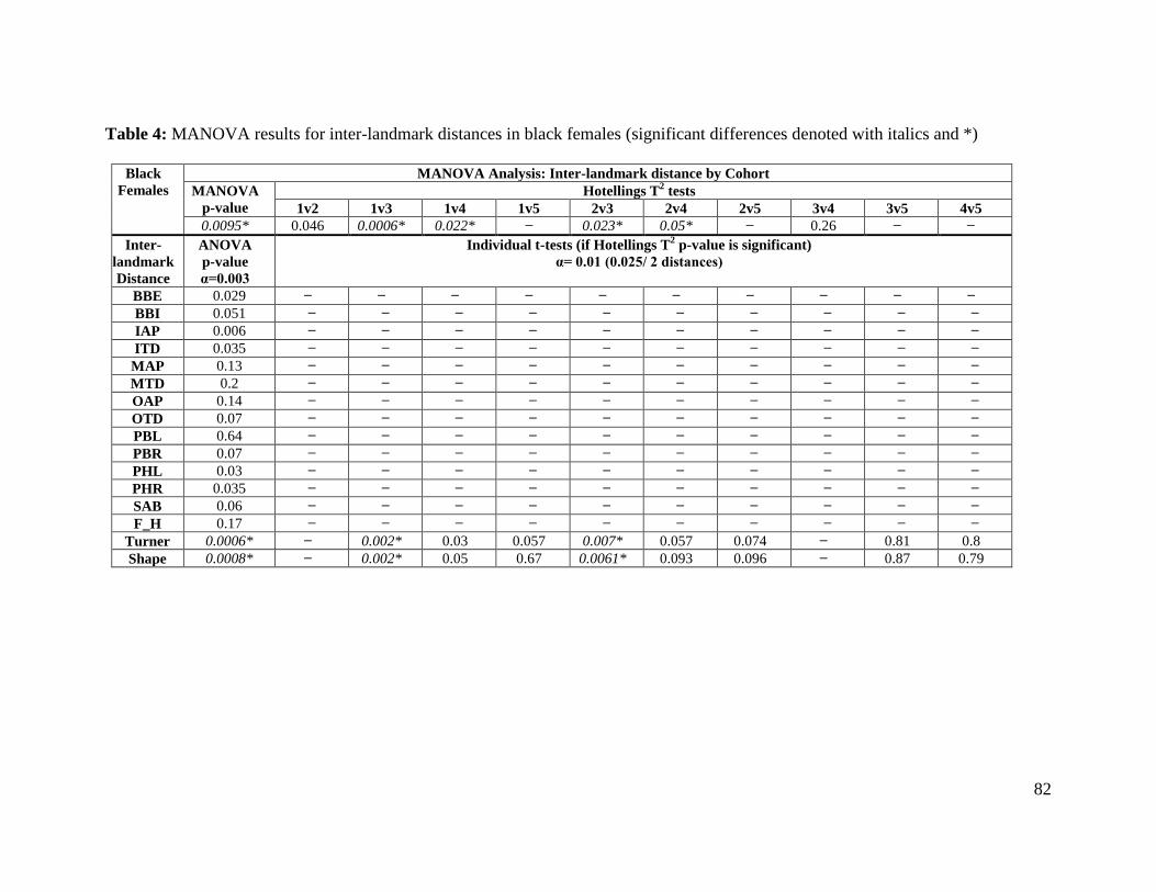
82
Table 4: MANOVA results for inter-landmark distances in black females (significant differences denoted with italics and *)
Black
Females
MANOVA Analysis: Inter-landmark distance by Cohort
MANOVA
p-value
Hotellings T2 tests
1v2 1v3 1v4 1v5 2v3 2v4 2v5 3v4 3v5 4v5
0.0095* 0.046 0.0006* 0.022* ̶ 0.023* 0.05* ̶ 0.26 ̶ ̶
Inter-
landmark
Distance
ANOVA
p-value
α=0.003
Individual t-tests (if Hotellings T2 p-value is significant)
α= 0.01 (0.025/ 2 distances)
BBE 0.029 ̶ ̶ ̶ ̶ ̶ ̶ ̶ ̶ ̶ ̶
BBI 0.051 ̶ ̶ ̶ ̶ ̶ ̶ ̶ ̶ ̶ ̶
IAP 0.006 ̶ ̶ ̶ ̶ ̶ ̶ ̶ ̶ ̶ ̶
ITD 0.035 ̶ ̶ ̶ ̶ ̶ ̶ ̶ ̶ ̶ ̶
MAP 0.13 ̶ ̶ ̶ ̶ ̶ ̶ ̶ ̶ ̶ ̶
MTD 0.2 ̶ ̶ ̶ ̶ ̶ ̶ ̶ ̶ ̶ ̶
OAP 0.14 ̶ ̶ ̶ ̶ ̶ ̶ ̶ ̶ ̶ ̶
OTD 0.07 ̶ ̶ ̶ ̶ ̶ ̶ ̶ ̶ ̶ ̶
PBL 0.64 ̶ ̶ ̶ ̶ ̶ ̶ ̶ ̶ ̶ ̶
PBR 0.07 ̶ ̶ ̶ ̶ ̶ ̶ ̶ ̶ ̶ ̶
PHL 0.03 ̶ ̶ ̶ ̶ ̶ ̶ ̶ ̶ ̶ ̶
PHR 0.035 ̶ ̶ ̶ ̶ ̶ ̶ ̶ ̶ ̶ ̶
SAB 0.06 ̶ ̶ ̶ ̶ ̶ ̶ ̶ ̶ ̶ ̶
F_H 0.17 ̶ ̶ ̶ ̶ ̶ ̶ ̶ ̶ ̶ ̶
Turner 0.0006* ̶ 0.002* 0.03 0.057 0.007* 0.057 0.074 ̶ 0.81 0.8
Shape 0.0008* ̶ 0.002* 0.05 0.67 0.0061* 0.093 0.096 ̶ 0.87 0.79

83
Figure 6: Plots of mean differences of significant variables in black females
60.00
75.00
90.00
105.00
120.00
1BF 2BF 3BF 4BF 5BF
Means of Turner
COHORT
Turner
-60.00
-40.00
-20.00
0.00
20.00
1BF 2BF 3BF 4BF 5BF
Means of Shape
COHORT
Shape
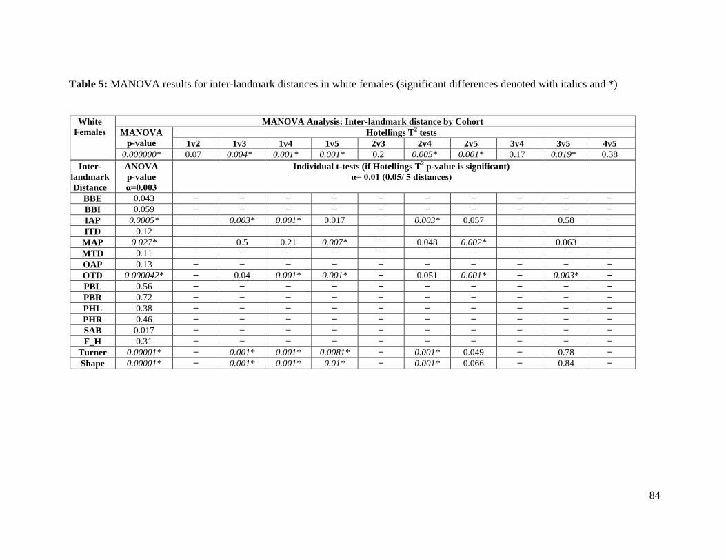
84
Table 5: MANOVA results for inter-landmark distances in white females (significant differences denoted with italics and *)
White
Females
MANOVA Analysis: Inter-landmark distance by Cohort
MANOVA
p-value
Hotellings T2 tests
1v2 1v3 1v4 1v5 2v3 2v4 2v5 3v4 3v5 4v5
0.000000* 0.07 0.004* 0.001* 0.001* 0.2 0.005* 0.001* 0.17 0.019* 0.38
Inter-
landmark
Distance
ANOVA
p-value
α=0.003
Individual t-tests (if Hotellings T2 p-value is significant)
α= 0.01 (0.05/ 5 distances)
BBE 0.043 ̶ ̶ ̶ ̶ ̶ ̶ ̶ ̶ ̶ ̶
BBI 0.059 ̶ ̶ ̶ ̶ ̶ ̶ ̶ ̶ ̶ ̶
IAP 0.0005* ̶ 0.003* 0.001* 0.017 ̶ 0.003* 0.057 ̶ 0.58 ̶
ITD 0.12 ̶ ̶ ̶ ̶ ̶ ̶ ̶ ̶ ̶ ̶
MAP 0.027* ̶ 0.5 0.21 0.007* ̶ 0.048 0.002* ̶ 0.063 ̶
MTD 0.11 ̶ ̶ ̶ ̶ ̶ ̶ ̶ ̶ ̶ ̶
OAP 0.13 ̶ ̶ ̶ ̶ ̶ ̶ ̶ ̶ ̶ ̶
OTD 0.000042* ̶ 0.04 0.001* 0.001* ̶ 0.051 0.001* ̶ 0.003* ̶
PBL 0.56 ̶ ̶ ̶ ̶ ̶ ̶ ̶ ̶ ̶ ̶
PBR 0.72 ̶ ̶ ̶ ̶ ̶ ̶ ̶ ̶ ̶ ̶
PHL 0.38 ̶ ̶ ̶ ̶ ̶ ̶ ̶ ̶ ̶ ̶
PHR 0.46 ̶ ̶ ̶ ̶ ̶ ̶ ̶ ̶ ̶ ̶
SAB 0.017 ̶ ̶ ̶ ̶ ̶ ̶ ̶ ̶ ̶ ̶
F_H 0.31 ̶ ̶ ̶ ̶ ̶ ̶ ̶ ̶ ̶ ̶
Turner 0.00001* ̶ 0.001* 0.001* 0.0081* ̶ 0.001* 0.049 ̶ 0.78 ̶
Shape 0.00001* ̶ 0.001* 0.001* 0.01* ̶ 0.001* 0.066 ̶ 0.84 ̶

85
80.00
97.50
115.00
132.50
150.00
1WF 2WF 3WF 4WF 5WF
Means of IAP
COHORT
IAP
100.00
112.50
125.00
137.50
150.00
1WF 2WF 3WF 4WF 5WF
Means of MAP
COHORT
MA
P
80.00
100.00
120.00
140.00
160.00
1WF 2WF 3WF 4WF 5WF
Means of OTD
COHORT
OT
D
60.00
75.00
90.00
105.00
120.00
1WF 2WF 3WF 4WF 5WF
Means of Turner
COHORT
Tu
rne
r
-60.00
-40.00
-20.00
0.00
20.00
1WF 2WF 3WF 4WF 5WF
Means of Shape
COHORT
Sh
ap
e
Figure 7: Plots of mean differences of significant variables in white females

86
Table 6: MANOVA results for inter-landmark distances in black males (significant differences denoted with italics and *)
Black
Males
MANOVA Analysis: Inter-landmark distance by Cohort
MANOVA
p-value
Hotellings T2 tests
1v2 1v3 1v3b 1v4 1v5 2v3 2v3b 2v4 2v5 3v3b 3v4 3v5 3bv4 3bv5 4v5
0.000001* 0.002* 0.003* 0.043* 0.004* 0.001* 0.99 0.008* 0.007* 0.001* 0.014* 0.03* 0.0009* 0.41 0.024* 0.022*
Inter-
landmark
Distance
ANOVA
p-value
α=0.003
Individual t-tests (if Hotellings T2 p-value is significant)
α= 0.007 (0.05/ 7 distances)
BBE 0.00004* 0.006* 0.011 0.002* 0.28 0.002* ̶ 0.001* 0.47 0.1 0.001* 0.63 0.13 ̶ 0.001* 0.1
BBI 0.0002* 0.62 0.1 0.04 0.086 0.001* ̶ 0.002* 0.52 0.004* 0.008 0.64 0.013 ̶ 0.002* 0.067
IAP 0.049 ̶ ̶ ̶ ̶ ̶ ̶ ̶ ̶ ̶ ̶ ̶ ̶ ̶ ̶ ̶
ITD 0.00081* 0.612 0.83 0.008* 0.76 0.001* ̶ 0.004* 0.55 0.002* 0.018 0.7 0.004* ̶ 0.002* 0.002*
MAP 0.017 ̶ ̶ ̶ ̶ ̶ ̶ ̶ ̶ ̶ ̶ ̶ ̶ ̶ ̶ ̶
MTD 0.11 ̶ ̶ ̶ ̶ ̶ ̶ ̶ ̶ ̶ ̶ ̶ ̶ ̶ ̶ ̶
OAP 0.15 ̶ ̶ ̶ ̶ ̶ ̶ ̶ ̶ ̶ ̶ ̶ ̶ ̶ ̶ ̶
OTD 0.00013* 0.014 0.026 0.024 0.001 0.017 ̶ 0.2 0.002* 0.34 0.15 0.001* 0.31 ̶ 0.51 0.16
PBL 0.055 ̶ ̶ ̶ ̶ ̶ ̶ ̶ ̶ ̶ ̶ ̶ ̶ ̶ ̶ ̶
PBR 0.84 ̶ ̶ ̶ ̶ ̶ ̶ ̶ ̶ ̶ ̶ ̶ ̶ ̶ ̶ ̶
PHL 0.14 ̶ ̶ ̶ ̶ ̶ ̶ ̶ ̶ ̶ ̶ ̶ ̶ ̶ ̶ ̶
PHR 0.15 ̶ ̶ ̶ ̶ ̶ ̶ ̶ ̶ ̶ ̶ ̶ ̶ ̶ ̶ ̶
SAB 0.0027* 0.97 0.9 0.025 0.18 0.001* ̶ 0.034 0.15 0.001* 0.022 0.19 0.0008* ̶ 0.001* 0.51
F_H 0.15 ̶ ̶ ̶ ̶ ̶ ̶ ̶ ̶ ̶ ̶ ̶ ̶ ̶ ̶ ̶
Turner 0.0009* 0.059 0.02 0.70 0.12 0.001* ̶ 0.62 0.66 0.003* 0.5 0.87 0.0028* ̶ 0.032 0.068
Shape 0.0013* 0.064 0.03 0.84 0.12 0.001* ̶ 0.49 0.65 0.003* 0.40 0.83 0.0029* ̶ 0.026 0.061

87
200.00
225.00
250.00
275.00
300.00
1BM 2BM 3BM 3bBM 4BM 5BM
Means of BBE
COHORT
BB
E
180.00
205.00
230.00
255.00
280.00
1BM 2BM 3BM 3bBM 4BM 5BM
Means of BBI
COHORT
BB
I
95.00
105.00
115.00
125.00
135.00
1BM 2BM 3BM 3bBM 4BM 5BM
Means of ITD
COHORT
ITD
60.00
77.50
95.00
112.50
130.00
1BM 2BM 3BM 3bBM 4BM 5BM
Means of OTD
COHORT
OT
D
40.00
65.00
90.00
115.00
140.00
1BM 2BM 3BM 3bBM 4BM 5BM
Means of SAB
COHORT
SA
B
60.00
80.00
100.00
120.00
140.00
1BM 2BM 3BM 3bBM 4BM 5BM
Means of Turner
COHORT
Tu
rne
r
-60.00
-35.00
-10.00
15.00
40.00
1BM 2BM 3BM 3bBM 4BM 5BM
Means of Shape
COHORT
Sh
ap
e
Figure 8: Plots of mean differences of significant variables in black males
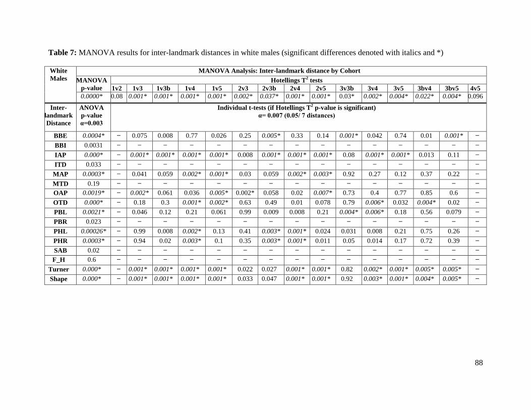
88
Table 7: MANOVA results for inter-landmark distances in white males (significant differences denoted with italics and *)
White
Males
MANOVA Analysis: Inter-landmark distance by Cohort
MANOVA
p-value
Hotellings T2 tests
1v2 1v3 1v3b 1v4 1v5 2v3 2v3b 2v4 2v5 3v3b 3v4 3v5 3bv4 3bv5 4v5
0.0000* 0.08 0.001* 0.001* 0.001* 0.001* 0.002* 0.037* 0.001* 0.001* 0.03* 0.002* 0.004* 0.022* 0.004* 0.096
Inter-
landmark
Distance
ANOVA
p-value
α=0.003
Individual t-tests (if Hotellings T2 p-value is significant)
α= 0.007 (0.05/ 7 distances)
BBE 0.0004* ̶ 0.075 0.008 0.77 0.026 0.25 0.005* 0.33 0.14 0.001* 0.042 0.74 0.01 0.001* ̶
BBI 0.0031 ̶ ̶ ̶ ̶ ̶ ̶ ̶ ̶ ̶ ̶ ̶ ̶ ̶ ̶ ̶
IAP 0.000* ̶ 0.001* 0.001* 0.001* 0.001* 0.008 0.001* 0.001* 0.001* 0.08 0.001* 0.001* 0.013 0.11 ̶
ITD 0.033 ̶ ̶ ̶ ̶ ̶ ̶ ̶ ̶ ̶ ̶ ̶ ̶ ̶ ̶ ̶
MAP 0.0003* ̶ 0.041 0.059 0.002* 0.001* 0.03 0.059 0.002* 0.003* 0.92 0.27 0.12 0.37 0.22 ̶
MTD 0.19 ̶ ̶ ̶ ̶ ̶ ̶ ̶ ̶ ̶ ̶ ̶ ̶ ̶ ̶ ̶
OAP 0.0019* ̶ 0.002* 0.061 0.036 0.005* 0.002* 0.058 0.02 0.007* 0.73 0.4 0.77 0.85 0.6 ̶
OTD 0.000* ̶ 0.18 0.3 0.001* 0.002* 0.63 0.49 0.01 0.078 0.79 0.006* 0.032 0.004* 0.02 ̶
PBL 0.0021* ̶ 0.046 0.12 0.21 0.061 0.99 0.009 0.008 0.21 0.004* 0.006* 0.18 0.56 0.079 ̶
PBR 0.023 ̶ ̶ ̶ ̶ ̶ ̶ ̶ ̶ ̶ ̶ ̶ ̶ ̶ ̶ ̶
PHL 0.00026* ̶ 0.99 0.008 0.002* 0.13 0.41 0.003* 0.001* 0.024 0.031 0.008 0.21 0.75 0.26 ̶
PHR 0.0003* ̶ 0.94 0.02 0.003* 0.1 0.35 0.003* 0.001* 0.011 0.05 0.014 0.17 0.72 0.39 ̶
SAB 0.02 ̶ ̶ ̶ ̶ ̶ ̶ ̶ ̶ ̶ ̶ ̶ ̶ ̶ ̶ ̶
F_H 0.6 ̶ ̶ ̶ ̶ ̶ ̶ ̶ ̶ ̶ ̶ ̶ ̶ ̶ ̶ ̶
Turner 0.000* ̶ 0.001* 0.001* 0.001* 0.001* 0.022 0.027 0.001* 0.001* 0.82 0.002* 0.001* 0.005* 0.005* ̶
Shape 0.000* ̶ 0.001* 0.001* 0.001* 0.001* 0.033 0.047 0.001* 0.001* 0.92 0.003* 0.001* 0.004* 0.005* ̶

89
220.00
245.00
270.00
295.00
320.00
1WM 2WM 3WM 3bWM 4WM 5WM
Means of BBE
COHORT
BB
E
80.00
100.00
120.00
140.00
160.00
1WM 2WM 3WM 3bWM 4WM 5WM
Means of IAP
COHORT
IAP
90.00
105.00
120.00
135.00
150.00
1WM 2WM 3WM 3bWM 4WM 5WM
Means of MAP
COHORT
MA
P
80.00
100.00
120.00
140.00
160.00
1WM 2WM 3WM 3bWM 4WM 5WM
Means of OAP
COHORT
OA
P
70.00
85.00
100.00
115.00
130.00
1WM 2WM 3WM 3bWM 4WM 5WM
Means of OTD
COHORT
OT
D
130.00
142.50
155.00
167.50
180.00
1WM 2WM 3WM 3bWM 4WM 5WM
Means of PBL
COHORT
PB
L
Figure 9: Plots of mean differences of significant variables in white males
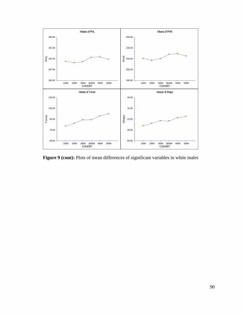
90
190.00
207.50
225.00
242.50
260.00
1WM 2WM 3WM 3bWM 4WM 5WM
Means of PHL
COHORT
PH
L
190.00
205.00
220.00
235.00
250.00
1WM 2WM 3WM 3bWM 4WM 5WM
Means of PHR
COHORT
PH
R
60.00
75.00
90.00
105.00
120.00
1WM 2WM 3WM 3bWM 4WM 5WM
Means of Turner
COHORT
Tu
rne
r
-60.00
-35.00
-10.00
15.00
40.00
1WM 2WM 3WM 3bWM 4WM 5WM
Means of Shape
COHORT
Sh
ap
e
Figure 9 (cont): Plots of mean differences of significant variables in white males
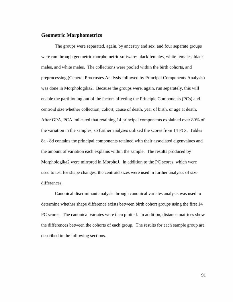
91
Geometric Morphometrics
The groups were separated, again, by ancestry and sex, and four separate groups
were run through geometric morphometric software: black females, white females, black
males, and white males. The collections were pooled within the birth cohorts, and
preprocessing (General Procrustes Analysis followed by Principal Components Analysis)
was done in Morphologika2. Because the groups were, again, run separately, this will
enable the partitioning out of the factors affecting the Principle Components (PCs) and
centroid size whether collection, cohort, cause of death, year of birth, or age at death.
After GPA, PCA indicated that retaining 14 principal components explained over 80% of
the variation in the samples, so further analyses utilized the scores from 14 PCs. Tables
8a - 8d contains the principal components retained with their associated eigenvalues and
the amount of variation each explains within the sample. The results produced by
Morphologika2 were mirrored in MorphoJ. In addition to the PC scores, which were
used to test for shape changes, the centroid sizes were used in further analyses of size
differences.
Canonical discriminant analysis through canonical variates analysis was used to
determine whether shape difference exists between birth cohort groups using the first 14
PC scores. The canonical variates were then plotted. In addition, distance matrices show
the differences between the cohorts of each group. The results for each sample group are
described in the following sections.

92
Tables 8 a-d: Principal Components retained for analyses
a) Black Females b) White Females
White
Females eigenvalue
percentage
of total
variance
explained
cumulative
variance
explained
PC 1 0.002303 27.10806 27.10806
PC 2 0.001593 18.75211 45.86017
PC 3 0.00064 7.534214 53.39438
PC 4 0.000562 6.61497 60.00935
PC 5 0.000387 4.553962 64.56331
PC 6 0.00037 4.356562 68.91988
PC 7 0.000307 3.613719 72.53359
PC 8 0.000246 2.897247 75.43084
PC 9 0.000213 2.505188 77.93603
PC 10 0.000186 2.186134 80.12216
PC 11 0.00016 1.887244 82.00941
PC 12 0.00014 1.647064 83.65647
PC 13 0.000122 1.434516 85.09099
PC 14 0.000112 1.321044 86.41203
c) Black Males d) White Males
White
Males eigenvalue
percentage
of total
variance
explained
cumulative
variance
explained
PC 1 0.001605 22.25604 22.25604
PC 2 0.00116 16.08472 38.34076
PC 3 0.000511 7.082668 45.42343
PC 4 0.000439 6.08902 51.51245
PC 5 0.000378 5.245871 56.75832
PC 6 0.000307 4.251158 61.00948
PC 7 0.000289 4.013938 65.02342
PC 8 0.000255 3.537707 68.56112
PC 9 0.000227 3.147784 71.70891
PC 10 0.000193 2.675848 74.38475
PC 11 0.00017 2.364355 76.74911
PC 12 0.000154 2.1325 78.88161
PC 13 0.000125 1.737469 80.61908
PC 14 0.000111 1.539796 82.15887
Black
Females eigenvalue
percentage
of total
variance
explained
cumulative
variance
explained
PC 1 0.0017 21.89668 21.89668
PC 2 0.001109 14.28148 36.17817
PC 3 0.000576 7.420575 43.59874
PC 4 0.000504 6.491402 50.09014
PC 5 0.000467 6.014315 56.10446
PC 6 0.000364 4.689333 60.79379
PC 7 0.000336 4.334345 65.12814
PC 8 0.000302 3.890841 69.01898
PC 9 0.000233 3.000992 72.01997
PC 10 0.000213 2.744888 74.76486
PC 11 0.00019 2.448211 77.21307
PC 12 0.000165 2.127672 79.34074
PC 13 0.000152 1.953225 81.29396
PC 14 0.000135 1.743024 83.03699
Black
Males eigenvalue
percentage
of total
variance
explained
cumulative
variance
explained
PC 1 0.001395 19.21764 19.21764
PC 2 0.000932 12.83164 32.04928
PC 3 0.000512 7.050644 39.09993
PC 4 0.000453 6.246161 45.34609
PC 5 0.000407 5.604851 50.95094
PC 6 0.00039 5.375956 56.3269
PC 7 0.000376 5.183867 61.51076
PC 8 0.000312 4.299617 65.81038
PC 9 0.000255 3.513901 69.32428
PC 10 0.000229 3.148464 72.47275
PC 11 0.000182 2.509522 74.98227
PC 12 0.000164 2.265436 77.2477
PC 13 0.000156 2.147218 79.39492
PC 14 0.000152 2.095746 81.49067

93
Shape: Black Females
Canonical variate analysis maximizes the amount of variation between groups.
After running the analysis on the five birth cohorts using the first 14 PCs, the first and
second canonical correlations were 0.67 and 0.42. The first two canonical variates (CVs)
represented 82.5% of the variation with the first CV responsible for over 65% of the total
variation. Only the eigenvalue associated with the CV1 was significant. Canonical
variate plots are shown in Figure 10a and 10b and Figure 11; these plots show two
different perspectives of the data, but each exhibits the same tendency. After plotting the
CV1 and CV2, the cohorts were separated temporally with the cohorts aligning along the
first canonical variate in order of birth year. Cohort 5 was separated from the rest of the
cohorts along the CV2. Temporally, cohort 5 fell in line with cohort 3; however, this was
based on a single black female in cohort 5. CV2 appears to account for variation that is
present in Cohort 4 and 5, black females from the Bass Collection. Again, it needs to be
noted that there are very few individuals in these cohorts compared to the earlier cohorts.
The distances between the cohorts are shown in Table 9.
In order to visualize the morphological changes that are occurring along CV1,
illustrations were created in MorphoJ; these illustrations correspond to the plot shown in
Figure 11. The illustrations are shown in Figure 12. Landmark identifications of the
numbered points can be found in Table A13 in the appendix. These illustrations
illuminate the shape change that is occurring as landmarks shift. The birth canal,
specifically the inlet AP diameter, is lengthening as is the outlet transverse diameter
along CV1. In concert, the iliac flare is decreasing with later cohorts.
94
Figure 10a: Canonical plot of individual black females Figure 10b: Canonical plot of cohort means of black females
-2.5
-1.2
0.2
1.5
-2.0 0.3 2.7 5.0
1BF
2BF
3BF
4BF
5BF
Can2
Can1
-4.00
-2.00
0.00
2.00
4.00
-4.00 -1.50 1.00 3.50 6.00
Canonical-Variates Scores
Score2
Sc
ore
1
COHORT
1BF2BF3BF4BF5BF

95
Figure 11: Canonical plot of individual black females produced in MorphoJ
Table 9: Distance matrix between black female cohorts, significance denoted by italics
Cohort 1BF 2BF 3BF 4BF
2BF 3.2349*
3BF 4.0153* 3.2864*
4BF 9.1047* 8.8938* 8.8870*
5BF 14.2316* 13.1444* 13.5818* 17.5315

96
Figure 12: Landmark shifts along first canonical variate in black females. The light blue
wireframe represents the starting form while the dark blue wireframe represents change
over canonical variate one (later cohorts). Landmark identifications of the numbered
points can be found in Table A13 in the appendix.
97
Shape: White Females
The first two canonical variates were significant in the white females and account
for nearly 80% of the variation between the cohorts. Canonical variate one accounted
for 56.8% of the total variation with a canonical correlation of 0.58. The second
canonical variate explained 22.7% of the variation and the canonical correlation is 0.41.
The plots of the canonical variates are shown in Figures 13a,b, and 14. Figures 13a and
13b were produced using NCSS and depict the individual values and the mean value,
respectively. Figure 14 was produced in Morphologika2. Similar to the black females,
CV1 separated the cohorts temporally. Again, cohort 5 was separated from the rest of the
groups on CV2, but with the white females, this CV is significant; CV2 was not
significant in the black females. While the separation in the black females was based on
a single individual, there are 11 white females in cohort 5. The distance matrix for the
white females is shown in Table 10; there is significant distance between each of the five
cohorts.
The morphological changes along CV1 and CV2 correspond to the plot shown in
Figure 14 are illustrated in Figures 15 and 16. These illustrations illuminate the shape
change that is occurring as landmarks shift. Like the black females, along CV1, the
outlet transverse diameter is lengthening and the inlet AP diameter greater in later
cohorts. The increase in the AP length was not as extreme as was found in the black
females. Also along CV1, there is a decrease in bi-iliac flare as well as an expansion of
the subpubic angle. In CV2, which appears to separate cohort 5, the angle of the iliac
blade appears to be the most significant difference.
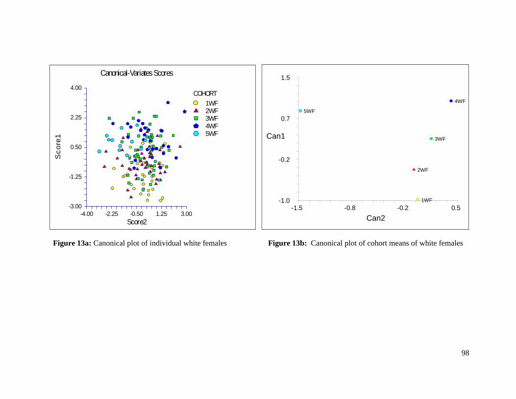
98
Figure 13a: Canonical plot of individual white females Figure 13b: Canonical plot of cohort means of white females
-1.0
-0.2
0.7
1.5
-1.5 -0.8 -0.2 0.5 1WF
2WF
3WF
4WF
5WF
Can2
Can1
-3.00
-1.25
0.50
2.25
4.00
-4.00 -2.25 -0.50 1.25 3.00
Canonical-Variates Scores
Score2
Sc
ore
1
COHORT
1WF2WF3WF4WF5WF
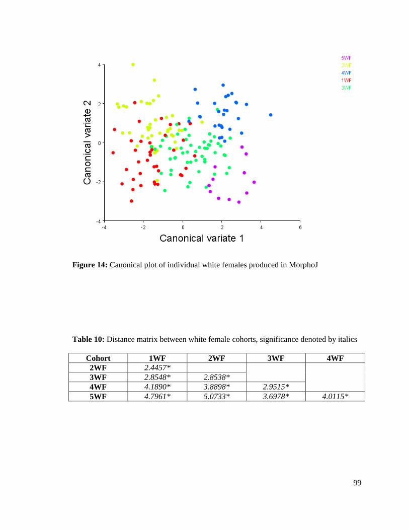
99
Figure 14: Canonical plot of individual white females produced in MorphoJ
Table 10: Distance matrix between white female cohorts, significance denoted by italics
Cohort 1WF 2WF 3WF 4WF
2WF 2.4457*
3WF 2.8548* 2.8538*
4WF 4.1890* 3.8898* 2.9515*
5WF 4.7961* 5.0733* 3.6978* 4.0115*

100
Figure 15: Landmark shifts along first canonical variate in white females. The light blue
wireframe represents the starting form while the dark blue wireframe represents change
over canonical variate one (later cohorts). Landmark identifications of the numbered
points can be found in Table A13 in the appendix.

101
Figure 16: Landmark shifts along second canonical variate in white females. The light
blue wireframe represents the starting form while the dark blue wireframe represents
change over canonical variate two. Landmark identifications of the numbered points can
be found in Table A13 in the appendix.
102
Shape: Black Males
After performing canonical variates analysis on the black males, only the first
canonical variate exhibited a significant eigenvalue. CV1 accounted for 55.8% of the
total variation between the cohorts with a canonical correlation of 0.64. While the second
CV did not have a significant eigenvalue, it accounted for 22.6% of the variation and has
a canonical correlation of 0.47. The plots of the canonical variates are shown in Figures
17a, b, and 18. Figures 17a and 17b were produced using NCSS and depict the
individual values and the mean value, respectively. Figure 18 was produced in
Morphologika2. The two programs show the same separation of groups. The distance
matrix shown in Table 11 indicates that there are significant differences between each
cohort.
Figure 19 illustrates the morphological changes along CV1. While the traditional
metrics indicated that the males were more variable than the females, the landmark shifts
in the black males appear to be comparable to those of the females. There was a decrease
in the bi-iliac flare, the sacral breadth, and the inlet transverse diameter. Also along
canonical variate one was an increase in the outlet transverse diameter. Additionally,
even though canonical variate two was not significant, it is shown in Figure 20 since
there is clearly a separation between the Bass black males and the other collections.
Along CV2, there is a decrease in the transverse diameter of the outlet, but the most
obvious difference is the anterior shift of the bi-iliac flare with an increase in iliac
breadth.

103
Figure 17a: Canonical plot of individual black males Figure 17b: Canonical plot of cohort means of black males
-3.00
-1.25
0.50
2.25
4.00
-4.00 -1.00 2.00 5.00 8.00
Canonical-Variates Scores
Score2
Score1
COHORT
1BM 2BM 3BM 3bBM 4BM 5BM
-1.0
-0.2
0.7
1.5
-0.5 0.2 0.8 1.5
1BM
2BM
3BM
3bBM
4BM
5BM
Can2
Can1
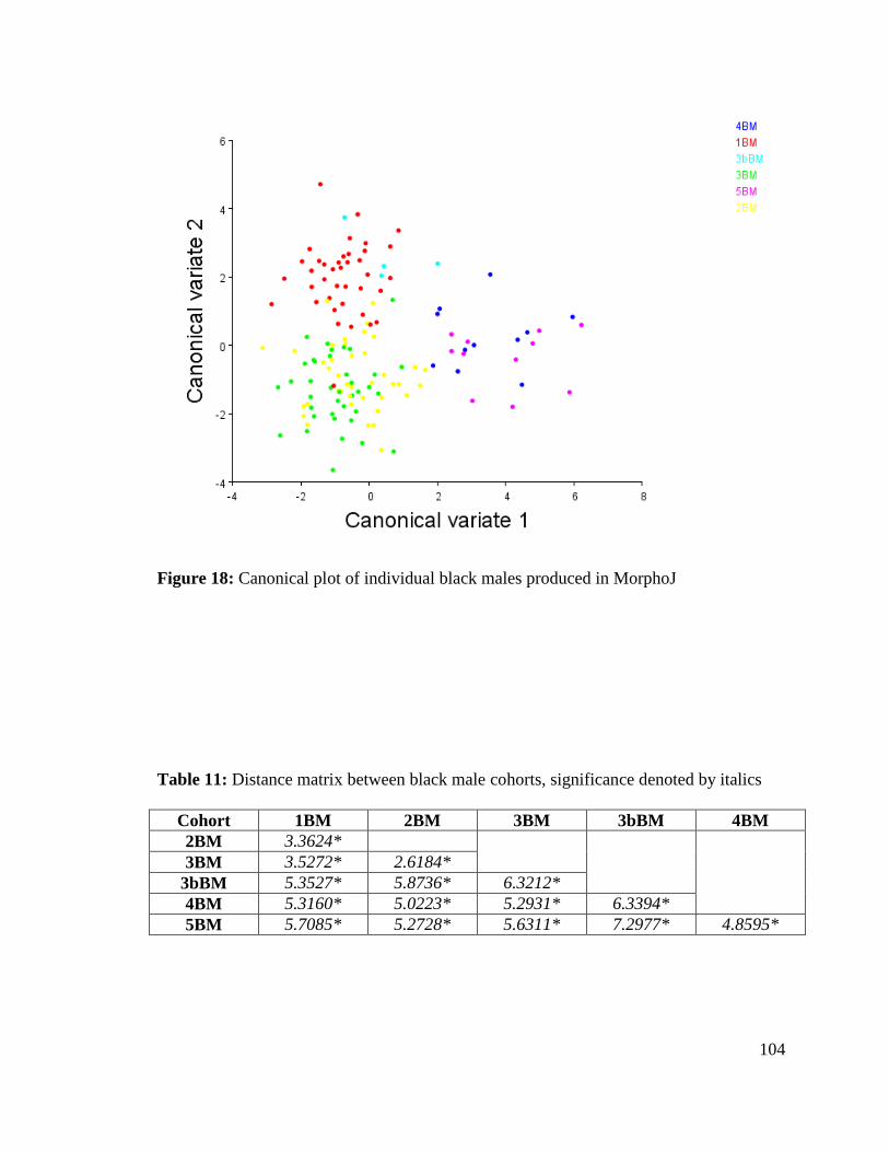
104
Figure 18: Canonical plot of individual black males produced in MorphoJ
Table 11: Distance matrix between black male cohorts, significance denoted by italics
Cohort 1BM 2BM 3BM 3bBM 4BM
2BM 3.3624*
3BM 3.5272* 2.6184*
3bBM 5.3527* 5.8736* 6.3212*
4BM 5.3160* 5.0223* 5.2931* 6.3394*
5BM 5.7085* 5.2728* 5.6311* 7.2977* 4.8595*

105
Figure 19: Landmark shifts along first canonical variate in black males. The light blue
wireframe represents the starting form while the dark blue wireframe represents change
over canonical variate one (later cohorts). Landmark identifications of the numbered
points can be found in Table A13 in the appendix.

106
Figure 20: Landmark shifts along second canonical variate in black males. The light
blue wireframe represents the starting form while the dark blue wireframe represents
change over canonical variate two. Landmark identifications of the numbered points can
be found in Table A13 in the appendix.

107
Shape: White Males
Two canonical variates were significant in separating the differences between the
cohorts in white males. Canonical variate one and canonical variates two account for
nearly 83% of the total variation with CV1 responsible for 60.6%. The canonical
correlations for the first two canonical variates were 0.66 and 0.47 respectively. Figures
21a, b, and 22 illustrate the canonical plots. Again, figures 21a and 21b were produced
using NCSS and depict the individual values and the mean value, respectively. Figure 22
was produced in Morphologika2. In the white males, CV1, again, separated the cohorts
temporally while CV2, like in the black males, separated the Bass males from the
Terry/Todd males. The distance between each cohort is significant and is depicted in
Table 12.
Similar to the black males, the morphology changes along canonical variate one
include an increase in the inlet AP and outlet transverse diameters as well as a decrease in
bi-iliac flare. In addition, the white males exhibit a decrease in the inlet transverse
diameter. Canonical variate two, which separates the Bass males from the other two
collections, involves an increase in bi-iliac flare, a decrease in the midplane transverse
diameter, and a medial movement of the posterior superior iliac spines. Illustrations of
the morphological shifts are shown in Figures 23 and 24. Traditional metrics indicated
that the white males were the most variable of the samples with several significant inter-
landmark distances; this is more difficult to state after examining the changes in shape
using geometric morphometry.
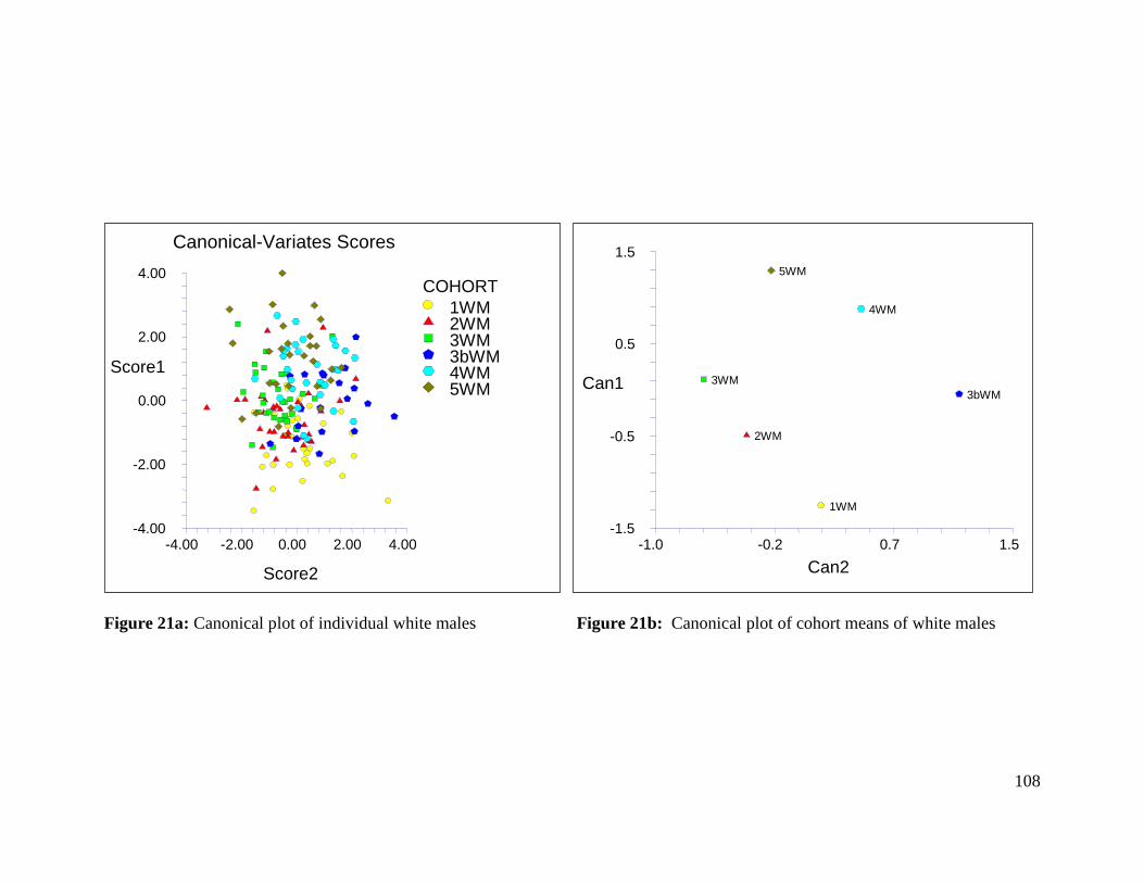
108
Figure 21a: Canonical plot of individual white males Figure 21b: Canonical plot of cohort means of white males
-4.00
-2.00
0.00
2.00
4.00
-4.00 -2.00 0.00 2.00 4.00
Canonical-Variates Scores
Score2
Score1
COHORT
1WM 2WM 3WM 3bWM 4WM 5WM
-1.5
-0.5
0.5
1.5
-1.0 -0.2 0.7 1.5
1WM
2WM
3WM 3bWM
4WM
5WM
Can2
Can1
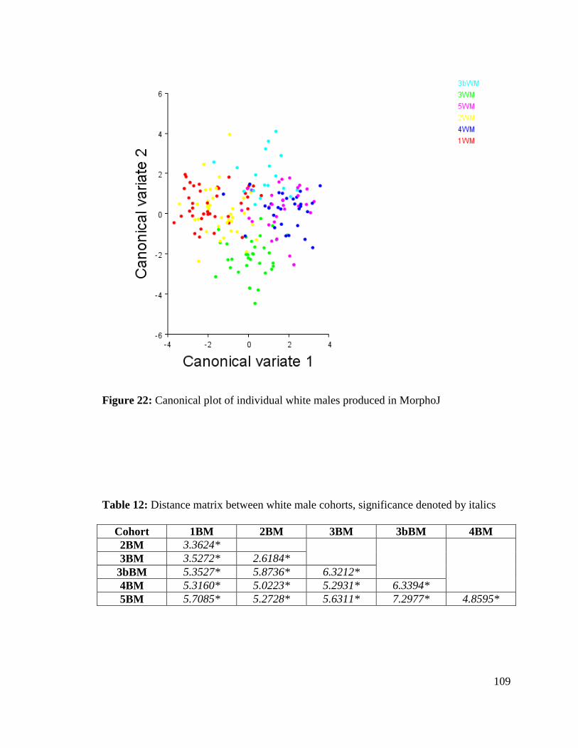
109
Figure 22: Canonical plot of individual white males produced in MorphoJ
Table 12: Distance matrix between white male cohorts, significance denoted by italics
Cohort 1BM 2BM 3BM 3bBM 4BM
2BM 3.3624*
3BM 3.5272* 2.6184*
3bBM 5.3527* 5.8736* 6.3212*
4BM 5.3160* 5.0223* 5.2931* 6.3394*
5BM 5.7085* 5.2728* 5.6311* 7.2977* 4.8595*

110
Figure 23: Landmark shifts along first canonical variate in white males. The light blue
wireframe represents the starting form while the dark blue wireframe represents change
over canonical variate one (later cohorts). Landmark identifications of the numbered
points can be found in Table A13 in the appendix.

111
Figure 24: Landmark shifts along second canonical variate in white males. The light
blue wireframe represents the starting form while the dark blue wireframe represents
change over canonical variate two. Landmark identifications of the numbered points can
be found in Table A13 in the appendix.
112
Shape: Collection Difference
Canonical variate analysis was next performed on each group to determine if
significant separation based on collection occurred along the canonical variates. These
plots are shown in Figures 25a,b – 28a,b. For each group, CV1 and CV2 were
significant in separating the groups by collection except for the black females; the black
females were only significantly separated along CV1. The first CV separated the groups
temporally; black females in Bass cohort 3 and 5 do not fit neatly into the temporal
division, this is again, perhaps, due to their small sample sizes. Canonical variate two
demarcates the collections into Terry versus Todd with the Bass samples straddling the
line. The white males are more clearly separated into three distinct collections along
CV2; this could be due to the more even sample sizes available in each of the cohort
break downs.
The results of the CVA on the cohorts separated by collection support the
decision to pool collections. While there are collection differences, the temporal
separation is much more significant.
Shape: Multivariate Regression Analysis
The 14 principal components were regressed on year of birth to determine which
PCs were significant between the cohorts. The results are shown in Table 13. While
several of the PCs show significance, they are built to maximize total sample variance.
Since the difference between the cohorts is of ultimate interest, the morphological
changes based on the PCs are of less concern than those based on the canonical variates
already discussed.
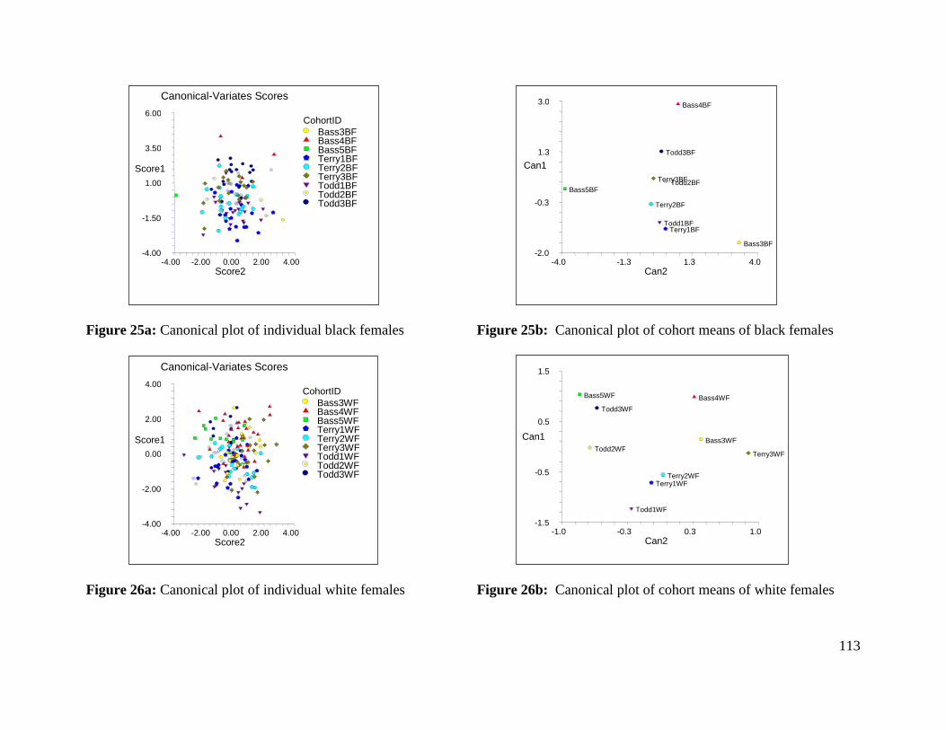
113
Figure 25a: Canonical plot of individual black females Figure 25b: Canonical plot of cohort means of black females
Figure 26a: Canonical plot of individual white females Figure 26b: Canonical plot of cohort means of white females
-4.00
-1.50
1.00
3.50
6.00
-4.00 -2.00 0.00 2.00 4.00
Canonical-Variates Scores
Score2
Score1
CohortID Bass3BF Bass4BF Bass5BF Terry1BF Terry2BF Terry3BF Todd1BF Todd2BF Todd3BF
-2.0
-0.3
1.3
3.0
-4.0 -1.3 1.3 4.0
Bass3BF
Bass4BF
Bass5BF
Terry1BF
Terry2BF
Terry3BF
Todd1BF
Todd2BF
Todd3BF
Can2
Can1
-4.00
-2.00
0.00
2.00
4.00
-4.00 -2.00 0.00 2.00 4.00
Canonical-Variates Scores
Score2
Score1
CohortID Bass3WF Bass4WF Bass5WF Terry1WF Terry2WF Terry3WF Todd1WF Todd2WF Todd3WF
-1.5
-0.5
0.5
1.5
-1.0 -0.3 0.3 1.0
Bass3WF
Bass4WF Bass5WF
Terry1WF Terry2WF
Terry3WF
Todd1WF
Todd2WF
Todd3WF
Can2
Can1

114
Figure 27a: Canonical plot of individual black males Figure 27b: Canonical plot of cohort means of black males
Figure 28a: Canonical plot of individual white males Figure 28b: Canonical plot of cohort means of white males
-4.00
-2.00
0.00
2.00
4.00
-4.00 -2.00 0.00 2.00 4.00
Canonical-Variates Scores
Score2
Score1
CohortID Bass3BM Bass4BM Bass5BM Terry1BM Terry2BM Terry3BM Todd1BM Todd2BM Todd3BM
-1.0
0.0
1.0
2.0
-1.0 -0.3 0.3 1.0
Bass3BM
Bass4BM Bass5BM
Terry1BM
Terry2BM Terry3BM
Todd1BM
Todd2BM Todd3BM
Can2
Can1
-1.5
-0.5
0.5
1.5
-1.5 -0.7 0.2 1.0
Bass3WM
Bass4WM
Bass5WM
Terry1WM
Terry2WM Terry3WM
Todd1WM
Todd2WM
Todd3WM
Can2
Can1
-4.00
-1.50
1.00
3.50
6.00
-3.00 -1.25 0.50 2.25 4.00
Canonical-Variates Scores
Score2
Score1
CohortID Bass3WM Bass4WM Bass5WM Terry1WM Terry2WM Terry3WM Todd1WM Todd2WM Todd3WM
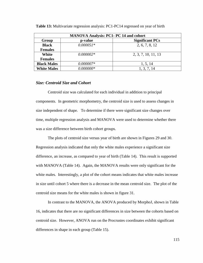
115
Table 13: Multivariate regression analysis: PC1-PC14 regressed on year of birth
MANOVA Analysis: PC1- PC 14 and cohort
Group p-value Significant PCs
Black
Females
0.000051* 2, 6, 7, 8, 12
White
Females
0.000002* 2, 3, 7, 10, 11, 13
Black Males 0.000007* 1, 5, 14
White Males 0.000000* 1, 3, 7, 14
Size: Centroid Size and Cohort
Centroid size was calculated for each individual in addition to principal
components. In geometric morphometry, the centroid size is used to assess changes in
size independent of shape. To determine if there were significant size changes over
time, multiple regression analysis and MANOVA were used to determine whether there
was a size difference between birth cohort groups.
The plots of centroid size versus year of birth are shown in Figures 29 and 30.
Regression analysis indicated that only the white males experience a significant size
difference, an increase, as compared to year of birth (Table 14). This result is supported
with MANOVA (Table 14). Again, the MANOVA results were only significant for the
white males. Interestingly, a plot of the cohort means indicates that white males increase
in size until cohort 5 where there is a decrease in the mean centroid size. The plot of the
centroid size means for the white males is shown in figure 31.
In contrast to the MANOVA, the ANOVA produced by MorphoJ, shown in Table
16, indicates that there are no significant differences in size between the cohorts based on
centroid size. However, ANOVA run on the Procrustes coordinates exhibit significant
differences in shape in each group (Table 15).

116
440.0
493.3
546.7
600.0
1800.0 1866.7 1933.3 2000.0
B
B
B
B
B
BB
B
B
B
B
B
B
B
B
B
B
B
B
B
B
B
B
B
BB
B
B
B
B
B
B
B
B
B
B
W
W
W
WW
W
W
WW
W
W
WW
W
WW
W
WW
W
W
W
W
W W
W
W
W
W
W
W
W
W
W
W
W
W
BB
B
B
B
B
B
B
B
BB
B
B
B
B
B
B
B
B
B
BB
B
B
B
B
B
B
B
BBB
B
B
B
B
B
B
B
W
W
W
W
WW
WW
W
W
W
W
W
W
W W
W
W
W
W
W
WW
W
WWW
W
W
W
W
W
W
WW
W
W
W
W
B
B
BB
B
B
BB B
BBB
B
BB
B
BB
B
B
B
B
B
B
B
BBB
B
BB
B
BB
B
BB
B
WWW
W
W
W
WW
WW
WW
W
W
W
W
WW
W
W
W
W
W
W
W
W
W
W
W
W
W
W
W
W
W W
W
W
W
W
W
W
W
W
WW
W
W
WW
W
W
BB
B
W
W
W
W
WW
W
WW
W
W
W
W
W
W
W W
W
W
W
W
W
W
W
WW
W
B
W
W
W
W
W
W
W
W W
WW
W
BirthYear
ce
ntr
oid
_siz
e
Figure 29: Plot of centroid size by birth-year for females
460.0
506.7
553.3
600.0
1840.0 1886.7 1933.3 1980.0
BB
B
B
B
BB
B
BB
B
B
B
B
B
B
B
B
B
B
B
B
B
B
B
B
B
B
B
B
B
B
B
BB
B B
B
B
W
W
W
W
W
W
W
W
W
W
WW
W
W
W
W
W
W
W
W
W
W
W
W
W
W
WW
W
W
W
WW
W W
W
W
B
B
B
B
B
B
BB
B
B
B
B
B
B
B
B
B
B
B
B
B
B
B
B
B
B
B
B
B
B
B
B
B
B B
BB
B
B
B
W W
W WWW
WW
WW
W
W
W
W
W
W
W
W
WW
W
W
W
W
W
W
W
W
W
W
WW
W
W
W
W
W
B
B
BB
B
B
B
B
B
B
B
B
B
B
B
B
B B
B
B
B
B
B
B
B
B
B
B
B
B
BB
B
B
B
BB
B
B
B
BW
W
W
W
W
W
WW
W
W
W
W
WWW
WW
W
W
WW
W
WW
W
WW
W
W
W
W
WW
W
W
W
W
W
WW
W
WW
W
W W
W
W
WW
W
B
B
BB
B
B
BB
BB
B
W
W
WW
W
W
W
W
WW
W
W
W
W
W
W
W
WW
W
WW
W
WW
W
W
W
W
B
B
BB
B
B
B
B
B
BB
W
W
WW
W
W
W
W
W
W
W
WW
W
W
W
W
W
WW
W
W
W
W
W
W
W
W
BirthYear
ce
ntr
oid
_siz
e
Figure 30: Plot of centroid size by birth-year for males

117
Table 14: Regression Analysis and MANOVA analyses of centroid size
Regression Analysis:
Centroid size by birth year
MANOVA: Centroid size by
cohort
Group p-value p-value
Black Females 0.110361 0.110361
White Females 0.490078 0.490078
Black Males 0.868750 0.868750
White Males 0.000978* 0.000978*
Figure 31: Plot of white male centroid mean by cohort
Table 15: ANOVA of centroid size and shape by cohort (MorphoJ)
ANOVA of Procrustes Coordinates
Group Centroid Size: p-value Shape: p-value
Black Females 0.8909 <.0001
White Females 0.6980 <.0001
Black Males 0.7409 <.0001
White Males 0.5553 <.0001
460.00
495.00
530.00
565.00
600.00
1WM 2WM 3WM 3bWM 4WM 5WM
Means of centroid_size
COHORT
CentroidSize

118
Size: Collection, Cause of Death, Age at Death
In order to determine if factors other than birth year/cohort were affecting the
centroid size, additional MANOVA were run on the samples using collection, cause of
death, and age at death as independent variables. The only significant difference in size
occurred among the white males in the MANOVA of collection. There was a significant
size difference between the Bass collection compared to the Terry and Todd collections.
The significant results are shown in Table 16 and Figure 32. This result is not surprising
after finding a significant difference in cohort size of white males and cohorts in the
previous section.
Table 16: MANOVA of centroid size by collection
Figure 32: Plot of white male centroid mean by collection
MANOVA Analysis: Centroid size by Collection
Group p-value
Black Females 0.649859
White Females 0.512975
Black Males 0.654403
White Males 0.000410*
460.00
495.00
530.00
565.00
600.00
Bass Terry Todd
Means of centroid_size
Collection
centroid_size

119
Size: Variable Selection
Finally, a McHenry’s variable selection was run on the centroid size to determine
which variable combination produce the most appropriate model for determining size.
Sex, ancestry, collection, year of birth, and year of birth were used for the first run.
Death type was added in a second variable selection; it was not included in the first run
since the death type was only defined for 273 of the 608 individuals used in the geometric
morphometric analyses. The causes of death were separated into two types: cardiac and
infectious. Those individuals who died from any type of heart or cardiovascular disease
fell under the first category while those who suffered from inflictions such as syphilis,
tuberculosis, influenza, or other contagious disease fell under the second category.
Variable selection was not run on the principal component scores because these scores
were produced through running the sex/ancestry groups separately which prevents the
PCs from being comparable and biased against the variables of sex and ancestry as
independent variables.
The model produced from the entire sample, excluding the variable of death type,
ancestry and sex were the first two variables included in the model followed by death
age. Year of birth and collection were added in the later models, but they do not
appreciably increase the R2 value of the model. This indicates that separating the sample
by ancestry and sex prior to testing for secular change was indeed essential. The early
entry of death age is likely an artifact of the ages of the samples included in the
collections; plots of the age at death in each collection can be found in the appendix. The
models are shown in Tables 17 and 18.

120
With the addition of death type, death age becomes more prominent in the model.
This is due to the highly skewed distribution of age and type of death. Those dying of
cardiac disease are far older than those individuals dying from infectious illness; plots
with age distributions can be found in the appendix. However, after death age is
explained, the next two variables are ancestry and sex which is similar to the first model
selection. While these results support the separation of the sample into sex/ancestry
groups, they also indicate that collection membership, and the environmental differences
associated with being in differing collections, have less effect on size than demographic
parameters.
Table 17: McHenry’s Variable Selection Using Centroid Size
Model Size
R-Squared R-Squared Change
Variable Names
1 0.288651 0.288651 Ancestry 2 0.319700 0.031049 Sex, Ancestry 3 0.335424 0.015724 Sex, Ancestry, DeathAge 4 0.343976 0.008552 BirthYear, Sex, Ancestry, DeathAge 5 0.344025 0.000049 Collection, BirthYear, Sex, Ancestry, DeathAge
Table 18: McHenry’s Variable Selection Using Centroid Size including death type
Model Size
R-Squared R-Squared Change
Variable Names
1 0.202544 0.202544 Ancestry 2 0.223327 0.020783 Ancestry, DeathAge 3 0.244683 0.021356 Sex, Ancestry, DeathAge 4 0.245775 0.001092 Sex, Ancestry, DeathAge, DeathType 5 0.245966 0.000191 Collection, Sex, Ancestry, DeathAge, DeathType 6 0.245970 0.000004 Collection, BirthYear, Sex, Ancestry, DeathAge, DeathType
121
Chapter 6
Discussion & Conclusion
The goal of this research was to determine if secular change occurred in the
modern human pelvis of individuals living in the United States who were born between
1840 and 1980. One hundred and forty years is a relatively short time to expect
significant changes to occur in the bony pelvis which is arguably one of the most
important skeletal elements in modern humans. However, there have been unprecedented
changes in technology, culture, health, and healthcare over the last century and a half in
addition to the novel environment that makes up the melting pot culture of the United
States. The evolution of the pelvis occurred because of changes in locomotion and
birthing; this has been studied extensively. Changes in the pelvis due to improved
nutrition, exogamy, decreased disease load, environment, and technology are all of
interest in understanding the current form and projected form of the modern human
pelvis.
Several hypotheses underlie this research. Overarching all of these questions was
the assumption that the pelvis would mirror changes found in other elements of the
skeleton. Stature, long bone length, and cranial base height have increased overtime with
improvements in the way of life in the United States. The change in allometry in the long
bones was also observed to change more than the length of bone taken singly. Also,
males, specifically white males, have been shown to be more variable than other groups
while black females are more stable (Jantz 1996; Meadows Jantz and Jantz 1999). In
addition to the assumption that the pelvis would experience change due to improved

122
conditions, it was also expected that technology would also play a role in altering the
pelvis - specifically, cesarean sections. Women who, historically, were unable to give
birth would die or their offspring would die. Infant mortality has experienced a dramatic
decrease as has maternal death during birth. With the adoption of cesarean sections and
their increased use, it was expected that some effect would result in the human bony
pelvis. Evolution of the human birth canal differs in males and females; parturition
required the females to adopt a less efficient bipedal form. If the selection pressure of
parturition was relaxed, perhaps bipedalism would shift the female morphology to one
more similar to that expressed in males. The results of this study were both expected and
contradictory based on these assumptions.
Initial Testing
Sex and ancestry differences were expected. Measurements were collected with
the intention of splitting the groups into samples based on ancestry and sex. The
significant differences between these demographic groups supported their separation.
Males were more variable than the females, and this also fit with previous studies. This
was true when comparing across collections. The Hamann-Todd and Terry individuals
were more similar to each other than they were to the Bass individuals; however, the
differences between the females of the same cohort were not significant while the Bass
males were significantly bigger than the other collections in the same cohort. This was
not surprising. The Hamann-Todd and Terry collections have similar history. Each was
created from an anatomical collection made of dissected cadaveric remains of largely
lower income or unclaimed individuals while the Bass collection is predominantly made

123
up of individuals who were family or self donated. Again, the stability of the female
form enabled the collections to be pooled while the Bass males were separated from the
Terry and Hamann-Todd males.
Body & Pelvis Size
Initially, the non-significant change found in femoral head diameter was a
surprise; however, this result is largely consistent with those found in Cridlin’s research
(2007). Because the secular change of the femoral head was determined to be
statistically insignificant, accounting for body size using the femoral head was not useful
in this research. Clearly, body size has increased; however, the femur head diameter may
better reflect body mass (or perhaps lean body mass) rather than stature. However, since
the differences in raw inter-landmark distances were of interest in this study of secular
changes, accounting for changes in body size is likely counterproductive to the aim of
this research.
Centroid sizes indicated that only the white males are getting significantly bigger
in later cohorts, but all of the groups are changing in dimension in very similar ways.
Expected increases in os coxal height and width were not significant indicating that
increased stature may not necessarily lead to bigger pelves.
Pelvic Canal Shape
Using traditional metric analyses and 3D geometric morphometrics provided a
way to compare two different types of data and two different methods in their ability to
124
identify secular change. In this study of size and shape change, the two methods
supported each other. Secular change is occurring in the human bony pelvis. The
calculated measurements derived from the inter-landmark metrics (Turner’s Index and
Pelvic Shape) indicated that shape changes occurred between the cohorts and inter-
landmark distances significantly changed over time. However, not all of the distances
changed equally or in the same direction. Here, geometric morphometrics was better able
to illustrate the shape changes that had occurred over the 140 years.
In the literature review, the development of rotational birth was discussed. This
type of birthing mechanism is hypothesized to have developed because of the differences
in dimension between the inlet, midplane, and outlet of the female birth canal. The inlet
has the widest dimension in a transverse direction while the outlet is widest in an
anteroposterior direction. Additionally, malnutrition has been shown to further
complicate the birthing process by shortening the inlet AP dimension which makes
delivery of neonate even more difficult. Results of this research show that the
dimensions of the birth canal are shifting in a way to ease the constraint of the minimum
diameter. All females and the white males had significantly longer inlet AP diameters in
later cohorts, and all of the groups experienced increases in the outlet transverse
diameter. With the increasing outlet transverse diameter, an increase in the subpubic
angle was also significant in the females and the white males. The females showed no
corresponding increase in inlet transverse or outlet AP diameters. Thus, the shape
changes that were indicated in the metric analyses were supported by the 3D results. This
increase in AP diameter of the inlet supports the hypothesis that nutrition has improved
over the last 140 years, but it also questions the effect cesareans are having on the birth

125
canal. Perhaps technology does have a negative impact on the pelvic canal, but this study
sample only includes individuals with birth years earlier than 1983 which precedes the
regular use of cesarean sections during difficult delivery. The increase in cesarean
sections includes many that are not due to pelvic canal size, and perhaps the results will
continue to disprove those found in Germany. Expanding the samples to include later
birth years is a future direction for this research as it trying to include women with
documented cesarean births.
An interesting finding in this research was the decrease in bi-iliac breadth of the
cohorts in each of the groups. While pelvic breath has been shown to correspond to the
climatic differences (Mayr 1956) , this decrease cannot be completely explained by
differences in climate. In the males, there is a decreasing trend in the Terry/Hamann-
Todd males that is mirrored in the Bass males. So, while the decrease is altered by
collection, the overall trend is a decrease in bi-iliac breadth. The females also experience
this decrease, but the decrease is not altered by collection membership. Bipedal
locomotion is more efficient as the iliac blades flare because the flare makes the
attachment site for the abductor muscles more lateral; this increases their mechanical
advantage during locomotion, also puts less pressure on femoral head (Delprete 2006;
Lovejoy 1988).
This decrease in flare is perplexing. Perhaps the decrease in locomotion and
increased dependence on technology offsets the need to maintain bipedal efficiency.
Another possibility is that the decrease in flare is a result of cultural preference. Narrow
hips are considered by some in the United States to be a preferred body type; given the
heritability of bi-iliac breadth, culture may be the cause of this alteration of the bony

126
pelvis. The decrease in flare may also be a result of increased stature. In order to
maintain body proportion (the body has been modeled as a cylinder), secular changes in
height could be causing this decrease in the bi-iliac breadth (Ruff 1991).
Conclusion
There is secular change occurring in the human bony pelvis. Significant changes
in shape were shown through both metric and geometric methods using both inter-
landmark distances and coordinate data. The parallel changes across cohorts in all of the
groups indicate that the changes in the bony pelvis can be explained as a result of
improved nutrition and environment. This environment likely includes a variety of
factors (exogamy, lifestyle, health, economics, etc.) that are difficult to tease apart.
However, this improved environment was experienced when these individuals were
neonates and growing children. Increases in the AP diameter are altered by early
childhood nutrition and activity. The increases in both the Turner’s Index and the
calculated Pelvic Shape indicate a decreased occurrence of android shaped pelvic canals.
The expansion of the canal also indicates an improvement in environment. Strenuous
activity experienced by young people results in the small, triangular shaped inlet.
Further study is needed to determine if the secular change of the pelvis will level
off like the increases in stature. Increasing sample sizes of later birth cohorts in addition
to expanding the research to include scans of living women are two directions that may
begin to answer these questions.

127
Bibliography
128
Abitbol MM. 1987. Obstetrics and posture in pelvic anatomy. Journal of Human
Evolution 16(3):243-255.
Abitbol MM. 1995. Reconstruction of the STS 14 (Australopithecus africanus) pelvis.
American Journal of Physical Anthropology 96(2):143-158.
Abitbol MM. 1996. The shapes of the female pelvis. Contributing factors. J Reprod Med
41(4):242-250.
Abitbol MM, Taylor-Randall UB, Barton PT, and Thompson E. 1997. Effect of modern
obstetrics on mothers from Third-World countries. J Matern Fetal Med 6(5):276-
280.
Aiello LC, and Wells JCK. 2002. Energetics and the Evolution of the Genus Homo.
Annual Review of Anthropology 31(1):323-338.
Aiello LC, and Wheeler P. 1995. The Expensive-Tissue Hypothesis: The Brain and the
Digestive System in Human and Primate Evolution. Current Anthropology
36(2):199-221.
Allen JA, and 1877. The influence of physical conditions in the genesis of species.
Radical Rev 1:108-140.
Angel JL. 1976. Colonial to modern skeletal change in the U.S.A. American Journal of
Physical Anthropology 45(3):723-735.
Angel JL. 1982. A new measure of growth efficiency: Skull base height. American
Journal of Physical Anthropology 58(3):297-305.
Armelagos GJ, and Gerven DPV. 2003. A Century of Skeletal Biology and
Paleopathology: Contrasts, Contradictions, and Conflicts. American
Anthropologist 105(1):53-64.
Baker BJ, Dupras TL, and Tocheri MW. 2005. The osteology of infants and children.
College Station: Texas A&M University Press.
Berge C. 1994. How did the australopithecines walk? A biomechanical study of the hip
and thigh of Australopithecus afarensis. Journal of Human Evolution 26(4):259-
273.
Berge C, Orban-Segebarth R, and Schmid P. 1984. Obstetrical interpretation of the
australopithecine pelvic cavity. Journal of Human Evolution 13(7):573-587.
Bergmann C. 1847. Ueber die VemhÄltnisse der WÄrmeökonomie der Tiere zu ihrer
Grosse. Göttinger Studien:595–708.
129
Blumenberg B, Fristrup K, Holloway RL, Jacobs KH, Jerison HJ, Kitahara-Frisch J,
McGrew WC, Martin RD, Tarli SB, Vancata V and others. 1983. The Evolution
of the Advanced Hominid Brain [and Comments and Reply]. Current
Anthropology 24(5):589-623.
Boas F. 1912. Changes in the Bodily Form of Descendants of Immigrants. American
Anthropologist 14(3):530-562.
Bock RD, and Sykes RC. 1989. Evidence for continuing secular increase in height within
families in the United States. American Journal of Human Biology 1(2):143-148.
Bookstein FL. 1991. Morphmetric Tools for Landmark Data: Geometry and Biology.
New York: Cambridge University Press.
Caldwell WE, and Moloy HC. 1938. Anatomical Variations in the Female Pelvis: Their
Classification and Obstetrical Significance: (Section of Obstetrics and
Gynaecology). Proc R Soc Med 32(1):1-30.
Cameron N, editor. 2002. Human growth and development. Amsterdam: Academic Press.
Conroy GC, Weber GW, Seidler H, Recheis W, Nedden DZ, and Mariam JH. 2000.
Endocranial capacity of the Bodo cranium determined from three-dimensional
computed tomography. 113(1):111-118.
Cridlin S. 2007. Examination of secular change in the vertical head diameter of the
human femur in American males and females. Knoxville: University of
Tennessee.
Crompton RH, Wang W, Li Y, Gunther M, and Savage R. 1998. The mechanical
effectiveness of erect and "bent-hip, bent-knee" bipedal walking in
Australopithecus afarensis. Journal of Human Evolution 35(1):55-74.
Darwin C. 1874. The descent of man New York: H.M Caldwell.
Delprete HA. 2006. Secular changes in the morphology of the modern human pelvis and
the implications for human evolution [dissertation]. New Brunswick: Rutgers. 205
p.
Dubrova YE, Kurbatova OL, Kholod ON, and Prokhorovskaya VD. 1995. Secular
growth trend in two generations of the Russian population. Human Biology
v67(n5):p755(713).
Falk D. 1991. 3.5 Million years of hominid brain evolution. Seminars in Neuroscience
3(5):409-416.

130
Fazekas IG, and Kosa F. 1978. Forensic Fetal Osteology. Kerner E, translator. Budapest:
Akademiai Kiado.
Fenner JN. 2005. Cross-cultural estimation of the human generation interval for use in
genetics-based population divergence studies. American Journal of Physical
Anthropology 128(2):415-423.
Fischman J. 1994. Putting a New Spin on the Birth of Human Birth. Science
264(5162):1082-1083.
Ghosh JR, and Bandyopadhyay AR. 2005. A Study on Cormic Index among Semi-Urban
Bengalee Boys of West Bengal, India
Coll Antropol 29(1):33–36.
Gravlee CC, Bernard HR, and Leonard WR. 2003a. Boas's Changes in bodily form: the
immigrant study, cranial plasticity, and Boas's physical anthropology. American
anthropologist 105(2):326-332.
Gravlee CC, Bernard HR, and Leonard WR. 2003b. Heredity, environment, and cranial
form: a reanalysis of Boas's immigrant data. Biological anthropology : historical
perspectives on current issues, disciplinary connections, and future directions
105(1):125-138.
Greene DL, and Sibley L. 1986. Neandertal Public Morphology and Gestation Length
Revisited. Current Anthropology 27(5):517-518.
Greulich WW, and Thoms H. 1938. The dimensions of the pelvic inlet of 789 white
females. The Anatomical Record 72(1):45-51.
Hager LD. 1989. THE EVOLUTION OF SEX DIFFERENCES IN THE HOMINID
BONY PELVIS. Berkeley: University of California.
Harcourt-Smith WEH, and Aiello LC. 2004. Fossils, feet and the evolution of human
bipedal locomotion. Journal of anatomy 204(5):403-416.
Henneberg M. 1998. EVOLUTION OF THE HUMAN BRAIN: IS BIGGER BETTER?
Clinical & Experimental Pharmacology & Physiology 25(9):745.
Hintze J. 2006. NCSS 2004, PASS Trial, and GESS Trial Kaysville, UT.
Holloway RL. 1983. Cerebral brain endocast pattern of Australopithecus afarensis
hominid. Nature 303(5916):420-422.

131
Holloway RL. 2002. Head to Head with Boas: Did He Err on the Plasticity of Head
Form? Proceedings of the National Academy of Sciences of the United States of
America 99(23):14622-14623.
Hulse FS. 1962. Race as an Evolutionary Episode. American Anthropologist 64(5):929-
945.
Hunt DR, and Albanese J. 2005. History and demographic composition of the Robert J.
Terry anatomical collection. American Journal of Physical Anthropology
127(4):406-417.
Hunt KD. 1994. The evolution of human bipedality: ecology and functional morphology.
Journal of Human Evolution 26(3):183-202.
Jablonski NG, and Chaplin G. 1993. Origin of habitual terrestrial bipedalism in the
ancestor of the Hominidae. Journal of Human Evolution 24(4):259-280.
Jantz LM. 1996. Secular change and allometry in the long limb bones of Americans from
the mid 1700s through the 1970s [Ph.D.]. United States -- Tennessee: The
University of Tennessee.
Jantz RL. 2001. Cranial change in Americans: 1850-1975. J Forensic Sci 46(4):784-787.
Jantz RL, and Meadows Jantz L. 2000. Secular change in craniofacial morphology.
American Journal of Human Biology 12(3):327-338.
Jantz RL, and Owsley DW. 1984. Temporal changes in limb proportionality among
skeletal samples of Arikara Indians. Annals of human biology 11:157-163.
Jantz RL, and Willey PS. 1983. Temporal and geographic patterning of relative head
height in the central Plains and middle Missouri areas. Plains anthropologist
28(99):59-67.
Jolly CJ. 1970. Hadropithecus: A Lemuroid Small-Object Feeder. Man 5(4):619-626.
Kaltreider DF. 1951. The transverse diameter of the inlet. Am J Obstet Gynecol
62(1):163-166.
Katzmarzyk PT, and Leonard WR. 1998. Climatic influences on human body size and
proportions: Ecological adaptations and secular trends. American Journal of
Physical Anthropology 106(4):483-503.
Klepinger LL. 2001. Stature, maturation variation and secular trends in forensic
anthropology. J Forensic Sci 46(4):788-790.
132
Klingenberg CP. 2008. MorphoJ. Faculty of Life Sciences, University of Manchester,
UK.
Komlos J. 2003. Access to Food and the Biological Standard of Living: Perspectives on
the Nutritional Status of Native Americans. The American Economic Review
93(1):252-255.
Komlos J, and Lauderdale BE. 2007. Spatial correlates of US heights and body mass
indexes, 2002. Journal of biosocial science 39(1):59-78.
LaVelle M. 1995. Natural selection and developmental sexual variation in the human
pelvis. American Journal of Physical Anthropology 98(1):59-72.
Lehmann KJ, Wischnik A, Zahn K, and Georgi M. 1992. [Do the obstetrically relevant
bony pelvic measurements change? A retrospective analysis of computed
tomographic pelvic x-rays]. Rofo 156(5):425-428.
Leonard WR, and Robertson ML. 1992. Nutritional requirements and human evolution:
A bioenergetics model. American Journal of Human Biology 4(2):179-195.
Leonard WR, and Robertson ML. 1997. Comparative primate energetics and hominid
evolution. American Journal of Physical Anthropology 102(2):265-281.
Lestrel PE, and Read DW. 1973. Hominid cranial capacity versus time: A regression
approach. Journal of Human Evolution 2(5):405-411.
Lewin R. 1982. How Did Humans Evolve Big Brains? Science 216(4548):840-841.
Lovejoy CO. 1981. The Origin of Man. Science 211(4480):341-350.
Lovejoy CO. 1988. Evolution of human walking. Scientific American 259(5):118-125.
Lovejoy CO. 1993. Are we sexy because we're smart, or are we smart because we're
sexy. In: Rasmussen RT, editor. The Origin of Humans and Humanness: Bartlett
& Jones.
Lovejoy CO. 2005. The natural history of human gait and posture. Part 2. Hip and thigh.
Gait & posture 21(1):113-124.
Lovejoy CO. 2007. The natural history of human gait and posture. Part 3. The knee. Gait
& posture 25(3):325-341.
Lovejoy CO, Heiple KG, and Burstein AH. 1973. The gait of Australopithecus. American
Journal of Physical Anthropology 38(3):757-779.

133
Lovejoy CO, Suwa G, Spurlock L, Asfaw B, and White TD. 2009. The Pelvis and Femur
of Ardipithecus ramidus: The Emergence of Upright Walking. Science
326(5949):71-716.
MacLatchy LM. 1996. Another look at the australopithecine hip. Journal of Human
Evolution 31(5):455-476.
Mayr E. 1956. Geographical Character Gradients and Climatic Adaptation. Evolution
10(1):105-108.
McHenry HM. 1982. The Pattern of Human Evolution: Studies on Bipedalism,
Mastication, and Encephalization. Annual Review of Anthropology 11:151-173.
McHenry HM. 1986. The first bipeds: a comparison of theA. afarensis and A. africanus
postcranium and implications for the evolution of bipedalism. Journal of Human
Evolution 15(3):177-191.
McHenry HM, and Coffing K. 2000. Australopithecus to Homo: Transformations in
Body and Mind. Annual Review of Anthropology 29(1):125-146.
Meadows Jantz L, and Jantz RL. 1999. Secular change in long bone length and
proportion in the United States, 1800-1970. American Journal of Physical
Anthropology 110(1):57-67.
Mednick LW. 1955. The evolution of the human ilium. American Journal of Physical
Anthropology 13(2):203-216.
Nicholson C. 1945. The two main diameters at the brim of the female pelvis. Journal of
anatomy 79(Pt 3):131-135.
O'Higgins P, and Jones N. 2006. Morphologika2: Tools for statistical shape analysis.
Hull York Medical School.
O'Rahilly R, Müller F, Carpenter S, and Swenson R. 2009. Basic Human Anatomy: A
Regional Study of Human Structure (online version). Dartmouth Medical School.
Ousley SD. 2004. 3Skull. Version 2.1.111P.
Pennisi E. 1999. Human Evolution:Did Cooked Tubers Spur the Evolution of Big Brains?
Science 283(5410):2004-2005.
Prost JH. 1980. Origin of bipedalism. American Journal of Physical Anthropology
52(2):175-189.
Raustorp A, and Ludvigsson J. 2007. Secular trends of pedometer-determined physical
activity in Swedish school children. p 1824-1828.
134
Relethford JH. 2004. Boas and beyond: Migration and craniometric variation. Journal of
Human Evolution 16(4):379-386.
Richmond BG, Begun DR, and Strait DS. 2001. Origin of human bipedalism: The
knuckle-walking hypothesis revisited. Yearbook of Physical Anthropology
116(S33):70-105.
Rightmire GP. 2004. Brain size and encephalization in early to Mid-Pleistocene Homo.
American Journal of Physical Anthropology 124(2):109-123.
Roche AF. 1979. Secular Trends in Stature, Weight, and Maturation. Monographs of the
Society for Research in Child Development 44(3/4):3-27.
Rodman PS, and McHenry HM. 1980. Bioenergetics and the origin of hominid
bipedalism. American Journal of Physical Anthropology 52(1):103-106.
Rohlf FJ, and Slice D. 1990. Extensions of the Procrustes Method for the Optimal
Superimposition of Landmarks. Systematic Zoology 39(1):40-59.
Rosenberg K, and Trevathan W. 1995. Bipedalism and human birth: The obstetrical
dilemma revisited. Evolutionary Anthropology 4(5):161-168.
Rosenberg KR. 1992. The evolution of modern human childbirth. Yearbook of Physical
Anthropology 35(S15):89-124.
Rosenberg KR, and Travathan WR. 2001. The Evolution of Human Birth. Scientific
American 285(5):72.
Rosenberg KR, and Trevathan WR. 2007. An anthropological perspective on the
evolutionary context of preeclampsia in humans. Journal of Reproductive
Immunology 76(1-2):91-97.
Ruff C-B. 1995. Biomechanics of the hip and birth in early Homo. American Journal of
Physical Anthropology 98(4):527-574.
Ruff C. 1987. Sexual dimorphism in human lower limb bone structure: relationship to
subsistence strategy and sexual division of labor. Journal of human evolution
16(5):391-416.
Ruff CB. 1991. Climate and body shape in hominid evolution. Journal of Human
Evolution 21(2):81-105.
Scheuer L, and Black S. 2000. Developmental juvenile osteology. San Diego, CA;
London: Academic Press.
Scheuer L, and Black S. 2004. The Juvenile Skeleton. London

135
San Diego, CA: Elsevier Academic Press.
Schultz AH. 1949. Sex differences in the pelves of primates. American Journal of
Physical Anthropology 7(3):401-424.
Schwartz JH. 2007. Skeleton Keys: an introduction to human skeletal morphology,
development, and analysis. New York Oxford University Press.
Shipman P, Walker A, and Bichell D. 1985. The Human Skeleton. Cambridge, MA:
Harvard University Press. 343 p.
Slice DE. 2005. Modern Morphometrics in Physical Anthropology. Boston, MA: Kluwer
Academic / Plenum Publishers New York.
Slice DE. 2007. Geometric Morphometrics. Annual Review of Anthropology 36(1):261-
281.
Sparks CS, and Jantz RL. 2002. A Reassessment of Human Cranial Plasticity: Boas
Revisited. Proceedings of the National Academy of Sciences of the United States
of America 99(23):14636-14639.
Stanford CB. 2006. Arboreal bipedalism in wild chimpanzees: Implications for the
evolution of hominid posture and locomotion. American Journal of Physical
Anthropology 129(2):225-231.
Steckel RH, and Prince JM. 2001. Tallest in the World: Native Americans of the Great
Plains in the Nineteenth Century. The American Economic Review 91(1):287-
294.
Steckel RH, Rose JC, Larsen CS, and Walker PL. 2002. Skeletal health in the Western
Hemisphere from 4000 B.C. to the present. Evolutionary Anthropology
11(4):142-155.
Stern JT, and Susman RL. 1983. The locomotor anatomy of Australopithecus afarensis.
American Journal of Physical Anthropology 60(3):279-317.
Stewart DB. 1984. The pelvis as a passageway. I. Evolution and adaptations. Br J Obstet
Gynaecol 91(7):611-617.
Sylvester AD. 2006a. The Decoupling Hypothesis: A new idea for the origin of hominid
bipedalism. Anthropology. Knoxville: University of Tennessee.
Sylvester AD. 2006b. Locomotor decoupling and the origin of hominin bipedalism.
Journal of theoretical biology 242(3):581-590.
136
Synstelien JA. 2001. Differences in the os coxae between blacks and whites: a
musculoskeletal approach to human variation [MA]. Knoxville: University of
Tennessee. 108 p.
Tague RG. 1989. Variation in pelvic size between males and females. American Journal
of Physical Anthropology 80(1):59-71.
Tague RG. 1992. Sexual dimorphism in the human bony pelvis, with a consideration of
the Neandertal pelvis from Kebara cave, Israel. American Journal of Physical
Anthropology 88(1):1-21.
Tague RG. 1995. Variation in pelvic size between males and females in nonhuman
anthropoids. American Journal of Physical Anthropology 97(3):213-233.
Tague RG. 2000. Do big females have big pelves? American Journal of Physical
Anthropology 112(3):377-393.
Tague RG. 2007. Costal process of the first sacral vertebra: Sexual dimorphism and
obstetrical adaptation. American Journal of Physical Anthropology 132(3):395-
405.
Tague RG, and Lovejoy CO. 1986. The obstetric pelvis of A.L. 288-1 (Lucy). Journal of
Human Evolution 15(4):237-255.
Tardieu C. 1999. Ontogeny and phylogeny of femoro-tibial characters in humans and
hominid fossils: Functional influence and genetic determinism. American Journal
of Physical Anthropology 110(3):365-377.
Tardieu C, and Trinkaus E. 1994. Early ontogeny of the human femoral bicondylar angle.
American Journal of Physical Anthropology 95(2):183-195.
Trevathan W, and Rosenberg K. 2000. The shoulders follow the head: postcranial
constraints on human childbirth. Journal of Human Evolution 39(6):583-586.
Trevathan WR. 1996. The Evolution of Bipedalism and Assisted Birth. Medical
Anthropology Quarterly 10(2):287-290.
Turner W. 1885. The Index of the Pelvic Brim as a Basis of Classification. J Anat Physiol
20(Pt 1):125-143.
Vrba ES. 1996. Climate, Heterochrony, and Human Evolution. Journal of
Anthropological Research 52(1):1-28.
Walrath DE. 1997. Sexual Dimorphism of the Pelvis and Its Relationship to Birth in
Human Evolution (Reproduction): University of Pennsylvania.

137
Wang WJ, Crompton RH, Li Y, and Gunther MM. 2003. Energy transformation during
erect and `bent-hip, bent-knee' walking by humans with implications for the
evolution of bipedalism. Journal of Human Evolution 44(5):563-579.
Ward CV. 2002. Interpreting the posture and locomotion of Australopithecus afarensis:
Where do we stand? American Journal of Physical Anthropology 119(S35):185-
215.
Washburn SL. 1960. Tools and human evolution. Scientific American 203:63-75.
Weyl N. 1977. Pelvic Brim and Cranial Size. Mankind Quarterly 18(2):119.
Wheeler PE. 1991. The influence of bipedalism on the energy and water budgets of early
hominids. Journal of Human Evolution 21(2):117-136.
Wischnik A, Lehmann KJ, Zahn K, Georgi M, and Melchert F. 1992. [Changes in pelvic
anatomy in 8 decades--computerized tomography study of obstetrically relevant
pelvic measurements]. Z Geburtshilfe Perinatol 196(2):49-54.
Zelditch ML, Swiderski DL, Sheets HD, and Fink WL. 2004. Geometric Morphometrics
for Biologists: A Primer. London: Elsevier Academic Press.

138
Appendix
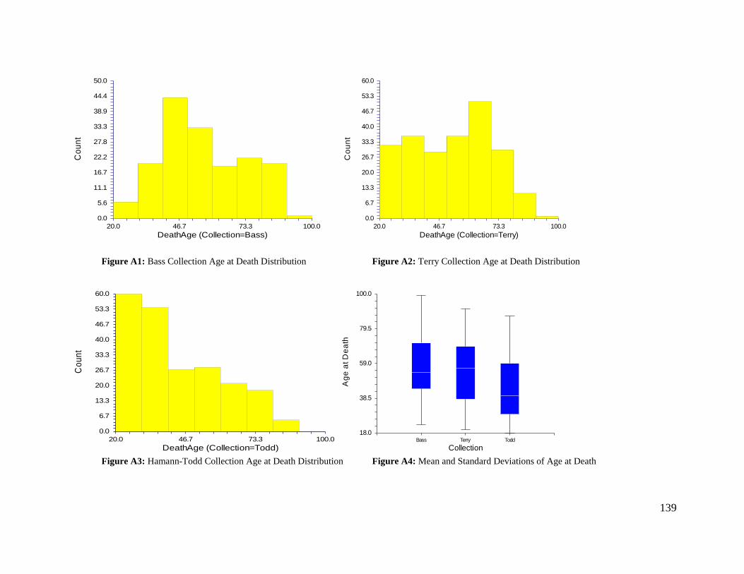
139
0.0
5.6
11.1
16.7
22.2
27.8
33.3
38.9
44.4
50.0
20.0 46.7 73.3 100.0
DeathAge (Collection=Bass)
Co
un
t
0.0
6.7
13.3
20.0
26.7
33.3
40.0
46.7
53.3
60.0
20.0 46.7 73.3 100.0
DeathAge (Collection=Terry)
Co
un
t
Figure A1: Bass Collection Age at Death Distribution Figure A2: Terry Collection Age at Death Distribution
0.0
6.7
13.3
20.0
26.7
33.3
40.0
46.7
53.3
60.0
20.0 46.7 73.3 100.0
DeathAge (Collection=Todd)
Co
un
t
18.0
38.5
59.0
79.5
100.0
Bass Terry Todd
Collection
Ag
e a
t D
ea
th
Figure A3: Hamann-Todd Collection Age at Death Distribution Figure A4: Mean and Standard Deviations of Age at Death

140
0.0
2.8
5.6
8.3
11.1
13.9
16.7
19.4
22.2
25.0
20.0 46.7 73.3 100.0
DeathAge (DeathType=Cardiac)
Co
un
t
0.0
8.9
17.8
26.7
35.6
44.4
53.3
62.2
71.1
80.0
20.0 46.7 73.3 100.0
DeathAge (DeathType=Infectious)
Co
un
t
Figure A5: Cardiac Death Age Distribution Figure A6: Infectious Death Age Distribution
18.0
38.5
59.0
79.5
100.0
Cardiac Infectious
Death Type
Ag
e a
t D
ea
th
Figure A7: Mean Age and Standard Deviation of Death Type

141
Table A1: Collection Comparisons for Black Females, Cohort 1&2
Black
Females
Cohort 1 Cohort 2
Normal Mean p-value
α =0.05
Normal Mean p-value
α =0.05 Terry Todd Terry Todd Terry Todd Terry Todd
BBE Yes Yes 255.84 251.7 0.4519 Yes Yes 251.15 247.25 0.47864
BBI Yes Yes 228.68 228.05 0.90316 Yes Yes 223.15 222.25 0.74149
IAP Yes Yes 104.74 108.95 0.20742 Yes Yes 109.7 110.1 0.90219
ITD Yes Yes 123.63 122 0.54001 Yes Yes 123.5 122 0.58871
MAP Yes Yes 124.63 128.7 0.1742 Yes Yes 127.85 123.85 0.23827
MTD Yes Yes 102.95 100.79 0.42201 Yes Yes 103.8 103.55 0.93074
OAP Yes Yes 119.37 122.85 0.30371 Yes Yes 122.85 118.8 0.25397
OTD Yes Yes 105.74 101.6 0.26559 Yes Yes 107.75 108.4 0.84964
PBL No No 146.42 142.35 0.85491 Yes Yes 144.8 143.35 0.57501
PBR Yes Yes 145.89 146.11 0.94915 Yes Yes 143.35 142.65 0.76538
PHL Yes Yes 197.21 196.85 0.91139 Yes Yes 193.75 192.35 0.68819
PHR Yes Yes 196.58 196.75 0.42201 Yes No 193.25 192.75 0.73477
SAB Yes Yes 106.32 103.75 0.30395 Yes Yes 105.1 103.6 0.51343
FH No Yes 42.53 42.77 0.844076 Yes Yes 41.67 41.94 0.741487
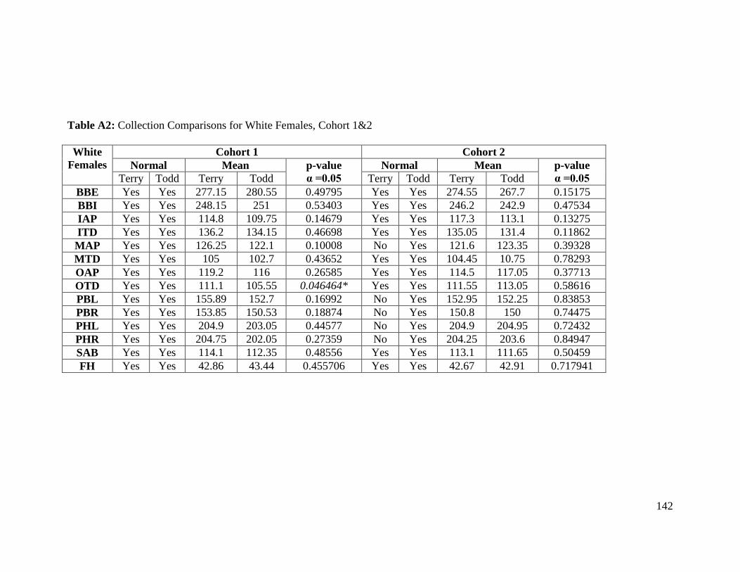
142
Table A2: Collection Comparisons for White Females, Cohort 1&2
White
Females
Cohort 1 Cohort 2
Normal Mean p-value
α =0.05
Normal Mean p-value
α =0.05 Terry Todd Terry Todd Terry Todd Terry Todd
BBE Yes Yes 277.15 280.55 0.49795 Yes Yes 274.55 267.7 0.15175
BBI Yes Yes 248.15 251 0.53403 Yes Yes 246.2 242.9 0.47534
IAP Yes Yes 114.8 109.75 0.14679 Yes Yes 117.3 113.1 0.13275
ITD Yes Yes 136.2 134.15 0.46698 Yes Yes 135.05 131.4 0.11862
MAP Yes Yes 126.25 122.1 0.10008 No Yes 121.6 123.35 0.39328
MTD Yes Yes 105 102.7 0.43652 Yes Yes 104.45 10.75 0.78293
OAP Yes Yes 119.2 116 0.26585 Yes Yes 114.5 117.05 0.37713
OTD Yes Yes 111.1 105.55 0.046464* Yes Yes 111.55 113.05 0.58616
PBL Yes Yes 155.89 152.7 0.16992 No Yes 152.95 152.25 0.83853
PBR Yes Yes 153.85 150.53 0.18874 No Yes 150.8 150 0.74475
PHL Yes Yes 204.9 203.05 0.44577 No Yes 204.9 204.95 0.72432
PHR Yes Yes 204.75 202.05 0.27359 No Yes 204.25 203.6 0.84947
SAB Yes Yes 114.1 112.35 0.48556 Yes Yes 113.1 111.65 0.50459
FH Yes Yes 42.86 43.44 0.455706 Yes Yes 42.67 42.91 0.717941
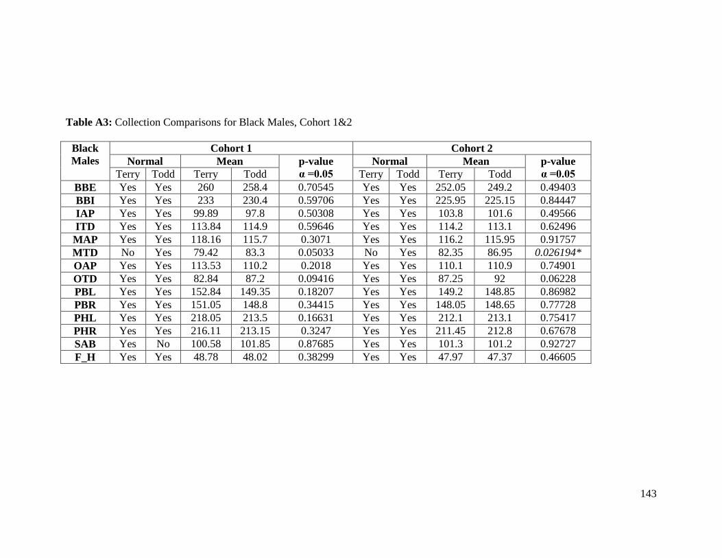
143
Table A3: Collection Comparisons for Black Males, Cohort 1&2
Black
Males
Cohort 1 Cohort 2
Normal Mean p-value
α =0.05
Normal Mean p-value
α =0.05 Terry Todd Terry Todd Terry Todd Terry Todd
BBE Yes Yes 260 258.4 0.70545 Yes Yes 252.05 249.2 0.49403
BBI Yes Yes 233 230.4 0.59706 Yes Yes 225.95 225.15 0.84447
IAP Yes Yes 99.89 97.8 0.50308 Yes Yes 103.8 101.6 0.49566
ITD Yes Yes 113.84 114.9 0.59646 Yes Yes 114.2 113.1 0.62496
MAP Yes Yes 118.16 115.7 0.3071 Yes Yes 116.2 115.95 0.91757
MTD No Yes 79.42 83.3 0.05033 No Yes 82.35 86.95 0.026194*
OAP Yes Yes 113.53 110.2 0.2018 Yes Yes 110.1 110.9 0.74901
OTD Yes Yes 82.84 87.2 0.09416 Yes Yes 87.25 92 0.06228
PBL Yes Yes 152.84 149.35 0.18207 Yes Yes 149.2 148.85 0.86982
PBR Yes Yes 151.05 148.8 0.34415 Yes Yes 148.05 148.65 0.77728
PHL Yes Yes 218.05 213.5 0.16631 Yes Yes 212.1 213.1 0.75417
PHR Yes Yes 216.11 213.15 0.3247 Yes Yes 211.45 212.8 0.67678
SAB Yes No 100.58 101.85 0.87685 Yes Yes 101.3 101.2 0.92727
F_H Yes Yes 48.78 48.02 0.38299 Yes Yes 47.97 47.37 0.46605
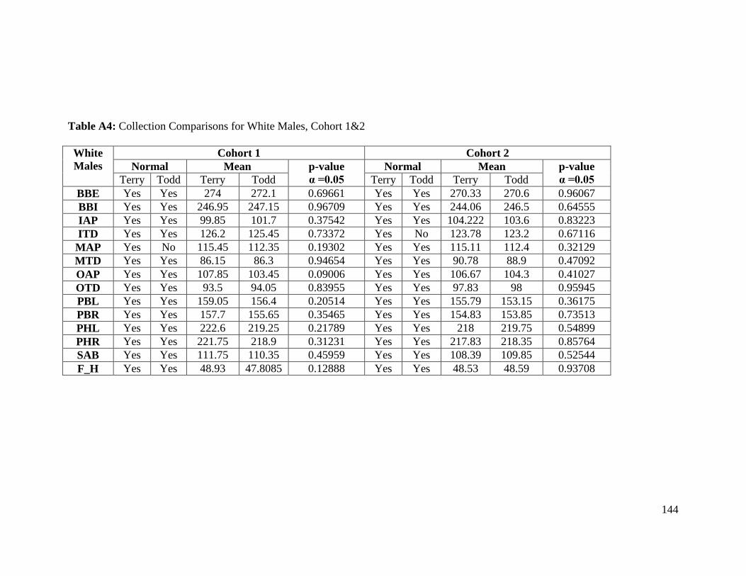
144
Table A4: Collection Comparisons for White Males, Cohort 1&2
White
Males
Cohort 1 Cohort 2
Normal Mean p-value
α =0.05
Normal Mean p-value
α =0.05 Terry Todd Terry Todd Terry Todd Terry Todd
BBE Yes Yes 274 272.1 0.69661 Yes Yes 270.33 270.6 0.96067
BBI Yes Yes 246.95 247.15 0.96709 Yes Yes 244.06 246.5 0.64555
IAP Yes Yes 99.85 101.7 0.37542 Yes Yes 104.222 103.6 0.83223
ITD Yes Yes 126.2 125.45 0.73372 Yes No 123.78 123.2 0.67116
MAP Yes No 115.45 112.35 0.19302 Yes Yes 115.11 112.4 0.32129
MTD Yes Yes 86.15 86.3 0.94654 Yes Yes 90.78 88.9 0.47092
OAP Yes Yes 107.85 103.45 0.09006 Yes Yes 106.67 104.3 0.41027
OTD Yes Yes 93.5 94.05 0.83955 Yes Yes 97.83 98 0.95945
PBL Yes Yes 159.05 156.4 0.20514 Yes Yes 155.79 153.15 0.36175
PBR Yes Yes 157.7 155.65 0.35465 Yes Yes 154.83 153.85 0.73513
PHL Yes Yes 222.6 219.25 0.21789 Yes Yes 218 219.75 0.54899
PHR Yes Yes 221.75 218.9 0.31231 Yes Yes 217.83 218.35 0.85764
SAB Yes Yes 111.75 110.35 0.45959 Yes Yes 108.39 109.85 0.52544
F_H Yes Yes 48.93 47.8085 0.12888 Yes Yes 48.53 48.59 0.93708

145
Table A5: Collection Comparisons for Black Females, Cohort 3
Black
Females
Cohort 3
Normal Mean ANOVA
p-value
Individual t-tests α =0.015
Bass Terry Todd Bass Terry Todd Bass/Ter Bass/Tod Tod/Ter
BBE Yes Yes Yes 261 244.35 241.15 0.37504 ̶ ̶ ̶
BBI Yes Yes Yes 228 220.8 217.4 0.64604 ̶ ̶ ̶
IAP Yes Yes Yes 108 112.55 111.45 0.82066 ̶ ̶ ̶
ITD Yes Yes Yes 119 118.35 118.1 0.98939 ̶ ̶ ̶
MAP Yes Yes No 121 124.9 118.25 0.08096 ̶ ̶ ̶
MTD Yes Yes Yes 99 100.6 98.32 0.6468 ̶ ̶ ̶
OAP Yes Yes Yes 112 120.55 111.45 0.020492* 0.42963 0.95514 0.0060*
OTD Yes Yes Yes 111 110.75 106.6 0.33365 ̶ ̶ ̶
PBL Yes Yes Yes 144 143.6 138.55 0.12961 ̶ ̶ ̶
PBR Yes Yes No 138 142.9 138.1 0.3951 ̶ ̶ ̶
PHL Yes Yes Yes 195 192.5 187.45 0.1817 ̶ ̶ ̶
PHR Yes Yes Yes 192 192.85 188 0.19079 ̶ ̶ ̶
SAB Yes Yes Yes 97 101.3 101.45 0.80824 ̶ ̶ ̶
F_H Yes Yes Yes 42.91 41.77 41 0.4262 ̶ ̶ ̶
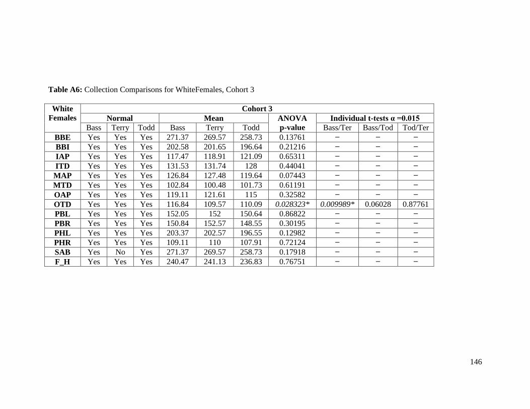
146
Table A6: Collection Comparisons for WhiteFemales, Cohort 3
White
Females
Cohort 3
Normal Mean ANOVA
p-value
Individual t-tests α =0.015
Bass Terry Todd Bass Terry Todd Bass/Ter Bass/Tod Tod/Ter
BBE Yes Yes Yes 271.37 269.57 258.73 0.13761 ̶ ̶ ̶
BBI Yes Yes Yes 202.58 201.65 196.64 0.21216 ̶ ̶ ̶
IAP Yes Yes Yes 117.47 118.91 121.09 0.65311 ̶ ̶ ̶
ITD Yes Yes Yes 131.53 131.74 128 0.44041 ̶ ̶ ̶
MAP Yes Yes Yes 126.84 127.48 119.64 0.07443 ̶ ̶ ̶
MTD Yes Yes Yes 102.84 100.48 101.73 0.61191 ̶ ̶ ̶
OAP Yes Yes Yes 119.11 121.61 115 0.32582 ̶ ̶ ̶
OTD Yes Yes Yes 116.84 109.57 110.09 0.028323* 0.009989* 0.06028 0.87761
PBL Yes Yes Yes 152.05 152 150.64 0.86822 ̶ ̶ ̶
PBR Yes Yes Yes 150.84 152.57 148.55 0.30195 ̶ ̶ ̶
PHL Yes Yes Yes 203.37 202.57 196.55 0.12982 ̶ ̶ ̶
PHR Yes Yes Yes 109.11 110 107.91 0.72124 ̶ ̶ ̶
SAB Yes No Yes 271.37 269.57 258.73 0.17918 ̶ ̶ ̶
F_H Yes Yes Yes 240.47 241.13 236.83 0.76751 ̶ ̶ ̶

147
Table A7: Collection Comparisons for Black Males, Cohort 3
Black
Males
Cohort 3
Normal Mean ANOVA
p-value
Individual t-tests α =0.015
Bass Terry Todd Bass Terry Todd Bass/Ter Bass/Tod Tod/Ter
BBE Yes Yes Yes 281.25 253.1 249.05 0.002393* 0.004624* 0.00052* 0.43115
BBI Yes Yes Yes 249.25 225.5 225.8 0.039156* 0.02488 0.01152* 0.95627
IAP Yes Yes Yes 109.25 105.85 102 0.22532 ̶ ̶ ̶
ITD Yes Yes Yes 123.75 113.7 114.35 0.08189 ̶ ̶ ̶
MAP Yes Yes Yes 129.25 118.55 115.95 0.017372* 0.011867* 0.01535 0.30899
MTD Yes Yes Yes 84 82.3 84.47 0.59428 ̶ ̶ ̶
OAP Yes Yes Yes 122 111.95 112.3 0.07953 ̶ ̶ ̶
OTD Yes Yes Yes 95.25 89.7 88.85 0.38126 ̶ ̶ ̶
PBL Yes Yes Yes 159.75 151.8 147.05 0.010205* 0.07776 0.00584* 0.0594
PBR Yes Yes No 159 150.95 145.15 0.01683 ̶ ̶ ̶
PHL Yes Yes Yes 227.5 217.65 212.45 0.044229* 0.11251 0.0219 0.15247
PHR Yes Yes Yes 226.5 217.25 211.9 0.042901* 0.12268 0.02171 0.13573
SAB Yes Yes Yes 108.75 100 102.1 0.0512 ̶ ̶ ̶
F_H Yes Yes Yes 50.669 48.82 47.83 0.09389 ̶ ̶ ̶

148
Table A8: Collection Comparisons for White Males, Cohort 3
White
Males
Cohort 3
Normal Mean ANOVA
p-value
Individual t-tests α =0.015
Bass Terry Todd Bass Terry Todd Bass/Ter Bass/Tod Tod/Ter
BBE Yes Yes Yes 283.95 265.43 266.3 0.001186* 0.003325* 0.00045* 0.88869
BBI Yes Yes Yes 252.7 240.24 240.85 0.034117* 0.03681 0.01557 0.9148
IAP Yes Yes Yes 113.15 107.21 110.15 0.1007 ̶ ̶ ̶
ITD Yes Yes Yes 127.15 123.43 123.1 0.18754 ̶ ̶ ̶
MAP Yes Yes Yes 117.9 118.86 116.9 0.70431 ̶ ̶ ̶
MTD Yes Yes Yes 85.1 88.14 85.55 0.4253 ̶ ̶ ̶
OAP No Yes Yes 110.65 112.29 111.1 0.49672 ̶ ̶ ̶
OTD Yes Yes Yes 96.1 96.07 97.3 0.899 ̶ ̶ ̶
PBL Yes Yes Yes 160.85 153.43 155 0.011900* 0.01667 0.01103* 0.54301
PBR Yes Yes Yes 158.5 154.29 153.72 0.13751 ̶ ̶ ̶
PHL Yes Yes Yes 227.3 219 222.35 0.06903 ̶ ̶ ̶
PHR Yes Yes Yes 226.25 218.93 221.6 0.11269 ̶ ̶ ̶
SAB Yes Yes Yes 110.85 107.14 110.5 0.15942 ̶ ̶ ̶
F_H Yes Yes Yes 49.04 47.89 4835 0.43697 ̶ ̶ ̶

149
Table A9: Descriptive Statistics Black Females, Cohort 4&5
Black
Females
Cohort 4 Cohort 5
Normal Mean s.d. Normal Mean s.d.
BBE Yes 246 13.11 BBE Yes 229 ̶
BBI Yes 218.33 14.05 BBI Yes 204 ̶
IAP Yes 126.33 10.69 IAP Yes 123 ̶
ITD Yes 126.67 11.15 ITD Yes 116 ̶
MAP Yes 124.33 7.23 MAP Yes 132 ̶
MTD Yes 105.33 6.5 MTD Yes 106 ̶
OAP Yes 115.33 9.07 OAP Yes 127 ̶
OTD Yes 113 2.65 OTD Yes 124 ̶
PBL Yes 145.33 4.04 PBL Yes 144 ̶
PBR Yes 145.67 4.04 PBR Yes 144 ̶
PHL Yes 198.67 191 PHL Yes ̶
PHR Yes 199.33 9.45 PHR Yes 189 ̶
SAB Yes 105.3 4.51 SAB Yes 92 ̶
F_H Yes 41.9 1.27 F_H Yes 40.4 ̶

150
Table A10: Descriptive Statistics White Females, Cohort 4&5
White
Females
Cohort 4 Cohort 5
Normal Mean s.d. Normal Mean s.d.
BBE Yes 269.93 16.73 BBE Yes 267.33 13.19
BBI Yes 241.73 15.94 BBI Yes 239.42 13.65
IAP Yes 122.1 7.85 IAP Yes 120.58 6.87
ITD Yes 130.47 8.54 ITD Yes 132 10.57
MAP Yes 126.73 8.49 MAP Yes 131.5 7.95
MTD Yes 100.93 11.32 MTD Yes 108.08 10.26
OAP Yes 117.23 8.82 OAP Yes 123.92 7.79
OTD Yes 117.13 12.35 OTD Yes 123.25 10.64
PBL Yes 153.5 7.07 PBL Yes 153.75 6.57
PBR Yes 152.52 7.88 PBR Yes 12.42 7.06
PHL No 203.07 9.25 PHL Yes 204 11.03
PHR Yes 203.2 9.36 PHR Yes 202.67 8.9
SAB Yes 108.77 8.23 SAB Yes 107.92 6.81
F_H Yes 41.94 1.75 F_H No 42.07 2.36
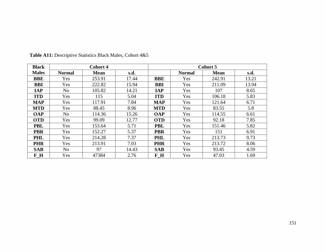
151
Table A11: Descriptive Statistics Black Males, Cohort 4&5
Black
Males
Cohort 4 Cohort 5
Normal Mean s.d. Normal Mean s.d.
BBE Yes 253.91 17.44 BBE Yes 242.91 13.21
BBI Yes 222.82 15.94 BBI Yes 211.09 13.94
IAP No 105.82 14.21 IAP Yes 107 8.65
ITD Yes 115 5.04 ITD Yes 106.18 5.83
MAP Yes 117.91 7.84 MAP Yes 121.64 6.71
MTD Yes 88.45 8.96 MTD Yes 83.55 5.8
OAP No 114.36 15.26 OAP Yes 114.55 6.61
OTD Yes 99.09 12.77 OTD Yes 92.18 7.85
PBL Yes 153.64 5.71 PBL Yes 151.46 5.82
PBR Yes 152.27 5.37 PBR Yes 151 6.91
PHL Yes 214.28 7.37 PHL Yes 213.73 9.73
PHR Yes 213.91 7.03 PHR Yes 213.72 8.06
SAB No 97 14.43 SAB Yes 93.45 4.59
F_H Yes 47384 2.76 F_H Yes 47.03 1.69
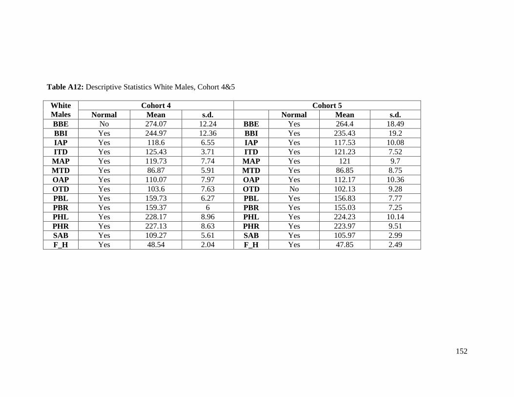
152
Table A12: Descriptive Statistics White Males, Cohort 4&5
White
Males
Cohort 4 Cohort 5
Normal Mean s.d. Normal Mean s.d.
BBE No 274.07 12.24 BBE Yes 264.4 18.49
BBI Yes 244.97 12.36 BBI Yes 235.43 19.2
IAP Yes 118.6 6.55 IAP Yes 117.53 10.08
ITD Yes 125.43 3.71 ITD Yes 121.23 7.52
MAP Yes 119.73 7.74 MAP Yes 121 9.7
MTD Yes 86.87 5.91 MTD Yes 86.85 8.75
OAP Yes 110.07 7.97 OAP Yes 112.17 10.36
OTD Yes 103.6 7.63 OTD No 102.13 9.28
PBL Yes 159.73 6.27 PBL Yes 156.83 7.77
PBR Yes 159.37 6 PBR Yes 155.03 7.25
PHL Yes 228.17 8.96 PHL Yes 224.23 10.14
PHR Yes 227.13 8.63 PHR Yes 223.97 9.51
SAB Yes 109.27 5.61 SAB Yes 105.97 2.99
F_H Yes 48.54 2.04 F_H Yes 47.85 2.49

153
Table A13: Landmark identification numbers used in geometric morphometric figures.
Landmark Number Landmark Point
1 superior pubic symphysis, center
2 ischial tuberosity, left
3 maximum pelvic height on iliac crest, left
4 transverse diameter point, right
5 auricular surface apex point, left
6 point on transverse line of S4 and S5
7 ischial spine, left
8 posterior superior iliac spine, right
9 anterior superior iliac spine, right
10 inferior pubic symphysis, center
11 apex of sacrum at S5, center
12 medial ischial tuberosity, left
13 medial ischial tuberosity, right
14 inner bi-iliac tubercle, left
15 inner bi-iliac tubercle, right
16 inferior ischial tuberosity, right
17 maximum pelvic height on iliac crest, right
18 ischial spine, right
19 posterior superior iliac spine, left
20 posterior inferior iliac spine, left
21 auricular surface apex point, right
22 transverse diameter point, left
23 anterior sacral promontory
24 bi-iliac tuberosity, left
25 bi-iliac tuberosity, right

154
Vita
Kathryn Roberts Dick was born October 6, 1976 in Bloomington, Illinois. After
living in both Wyoming and Florida, she graduated from Bloomington (Illinois) High
School in 1995. In May 1999, Kathryn received a Bachelor of Arts degree with honors in
History with minors in Biology and Chemistry from Bethel College, North Newton,
Kansas, and in July 1999, she married Darin Driscoll. Kathryn graduated with a Master
of Arts in the Social Sciences from the University of Chicago in June 2000. After having
two children, Kathryn returned to school in August 2004 and began her doctoral work at
the University of Tennessee. She received her PhD in Biological Anthropology in May
2010.