1

Sectoral real exchange rates and manufacturing exports:

A case study of Latin America

Thomas Goda*, Alejandro Torres** & Cristhian Larrahondo***1

Presented at the 25th FMM Conference, Berlin; 30 October 2021

Abstract

Standard theory considers the real exchange rate (RER) as an export determinant.

Accordingly, it is often argued that overvalued RER hamper economic growth. Most

prominently, the “New Developmentalism” school of thought contents that overvalued RER

are a key determinant of underdevelopment in Latin America; and that exchange rate

management is necessary to achieve an industrial equilibrium RER that enables exporters to

be competitive. However, a common limitation of cross-country evidence is the use of effective

(REER) or bilateral (BRER) RER indices, both of which have the same values across sectors.

The novel contributions of this paper are to exploit exchange rate variations across sectors by

constructing a unique sectoral bilateral RER index (SBRER) for 12 Latin American countries,

21 sectors and 38 trade partners, and to estimate empirically the effect of SBRER movements

on Latin American manufacturing exports during 2001-2018. The obtained results show that

the SBRER is a statistically significant determinant of aggregate manufacturing exports,

whereas the REER coefficient has an unexpected sign and the BRER appears not to be

significant. Moreover, sectoral export elasticities indicate that in Latin America mainly low-

technology sectors are affected by SBRER movements. Overall, these findings make evident

that it is important to consider sectoral heterogeneity regarding trade partners and production

costs when estimating RER export elasticities from a macroeconomic perspective. Moreover,

they indicate that in Latin America commodity price related RER appreciations mainly limit

the export growth of labor-intensive manufacturing sectors.

Keywords: Real Exchange Rate; Manufacturing Exports; Trade; Product Complexity; Latin

America

JEL Codes: F14, F31; O14

* School of Economics and Finance, Economics Department, Centro de Investigaciones Económicas y

Financieras (Cief), Universidad EAFIT, Medellin; tgoda@eafit.edu.co (corresponding autor)

** School of Economics and Finance, Economics Department, Centro de Investigaciones Económicas y

Financieras (Cief), Universidad EAFIT, Medellin; atorres7@eafit.edu.co.

*** School of Economics and Finance, Universidad EAFIT, Medellin; cdlarrahod@eafit.edu.co.

2

1. Introduction

Standard macroeconomic theory considers the real exchange rate (RER) as an indicator of the

average price competitiveness of firms. Accordingly, an appreciation (depreciation) of the

RER is expected to affect exports of a country negatively (positively). Considering this

relationship, the “New Developmentalism” school of thought contents that overvalued RER

are a key determinant of Latin American underdevelopment and that in middle-income

countries exchange rate management is necessary to achieve an industrial equilibrium RER

that enables exporters to be competitive, which in turn will foster economic growth (see e.g.,

Bresser-Pereira, 2016; 2018; 2020a; 2020b).

Single country studies that use firm-level data typically provide support for this expected

link between the RER and exports. For example, Greenaway et al. (2010), Berman et al.

(2012), Tang & Zhang (2012), Cheung & Sengupta (2013), Amiti et al., (2014), Li et al.

(2015), Fornero et al. (2020) and Dai et al. (2021) show that in Chile, China, Belgium, France,

India and the UK RER movements affect exports at the extensive (due to the entry/exit of

smaller and less productive firms) and intensive margin. However, especially for developing

countries, rich firm-level datasets are often not available and the empirical evidence that uses

aggregate data is more mixed with widely varying estimates of the elasticity of exports to RER

changes. For example, Thorbecke & Smith (2010) and Sekkat & Varoudakis (2000) find that

exchange rate movements affect the export performance of China and Sub-Saharan countries,

respectively, whereas Fang et al.’s (2006) results indicate that bilateral exports from Indonesia,

Japan, Korea, Philippines, Singapore and Taiwan to the USA are not affected by RER changes.

Moreover, Ahmed et al. (2017) and Kang & Dagli (2018) show for a panel of developed and

developing countries that the increasing integration of countries in global value chains has led

do a decrease of the RER elasticity of exports. Meanwhile the IMF (2015) provides evidence

to the contrary (i.e., the results indicate that the relationship between RER movements and

exports has remained relatively stable over time).

One common limitation of cross-country data studies is that they consider either a one-

dimensional real effective RER index (REER) or a two-dimensional bilateral RER index

(BRER). The REER considers inflation-adjusted averages that change over time but are

constant with regard to trade partners, while the BRER value is different for each trade partner

and year. A common limitation of both indices is that they assume that all industries within a

3

country have the same RER2, but industries can have heterogeneous RER movements when

they have different trade partners (Goldberg, 2004), distinct cost changes and/or diverging

degrees of price stickiness (see Carvalho & Nechio (2011) on the latter). The novel

contribution of this paper is to exploit the existing variation in terms of trade partners and cost

changes between sectors to reassess the relationship between RER movements and

manufacturing exports in Latin America, by constructing a sectoral bilateral RER index

(SBRER).

Latin America is an interesting case to establish whether the use of different exchange

rate measures matters when verifying the impact of RER movements on exports because

during the last commodity boom of 2003-2014 the debate about the potential adverse effects

of RER appreciation was revived in many countries of the region. More specifically, it is often

argued that the boom led to a Dutch disease phenomenon that harmed the manufacturing sector

of many countries in the region (see Ocampo, 2017). Moreover, the RER depreciation that

followed the end of the commodity boom did not lead to a surge of manufacturing exports –

the region’s percentage of manufacturing products in merchandise exports dropped by 0.9

points during 2014-2019, according to data from the World Bank (2020). Despite the

importance of this debate, we are not aware of a recent empirical paper that studies the

relationship between RER movements and Latin American manufacturing exports on a

regional scale.

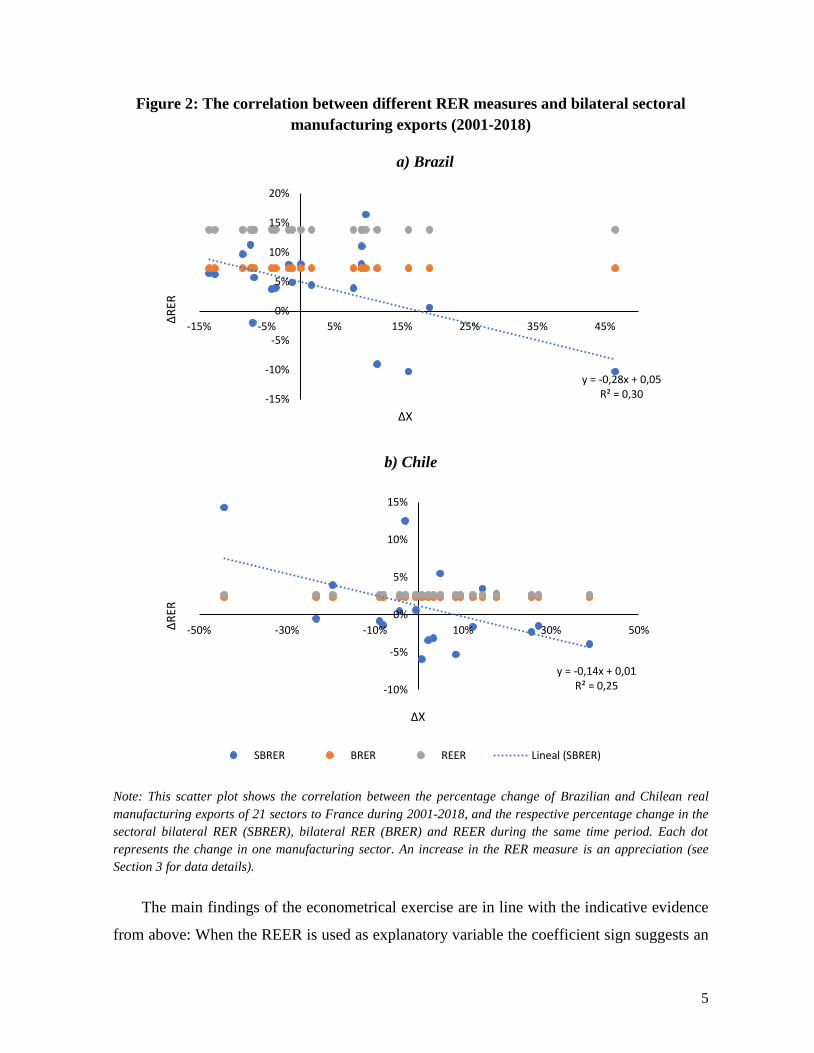
Contrary to the general perception, Figure 1 suggests that REER movements and Latin

American manufacturing export growth are not correlated, and that if any relationship exists

it is an inverse one (i.e., most countries experienced a REER appreciation coupled with an

increase in exports). This conclusion changes though when one accounts for sectoral

heterogeneity. Figure 2 shows the export growth of 21 Brazilian and Chilean manufacturing

industries to France and their respective REER, BRER and SBRER movements. It illustrates

that sectors within countries have distinct RER movements and that the correlation between

the SBRER and bilateral exports is negative (as theoretically expected), whereas there exists

no clear relationship between the REER and BRER and sectoral exports.

2 Please note that, according to Mayer & Steingress (2020), another limitation of existing REER indices is that

they are aggregated by using functional form assumptions and trade flow weighting schemes that are not

consistent with structural gravity equations. However, the resulting RER elasticity bias is minor (approx. 1%).

4

Figure 1: The non-correlation between the REER and Latin American manufacturing

exports (2001-2018)

Note: This scatter plot shows the non-correlation between the percentage change in the REER and manufacturing

exports (in constant USD) of 12 Latin American countries for the period 2001-2018. An increase in the REER

represents an appreciation (see Section 3 for data details).

Of course, this illustration is only indicative that sectoral RER movements matter for

export growth. To reassess the relationship more formally, this paper first presents a

modification of Reinhart’s (1995) trade model to show that, theoretically, sectoral

heterogeneity matters for the bilateral exports of developing countries. In a second step, a

three-dimensional SBRER for 12 Latin American countries is calculated, which considers the

variation of producer price differentials and bilateral nominal exchange rates across 21 sectors,

38 trade partners and 18 years. Finally, panel data regressions are used to verify the impact of

these 172,368 distinct SBRER observations on Latin American manufacturing exports, and

the results are compared with those obtained when using standard REER and BRER measures.

ARG

BOL

BRA

CHL

COL

CRI

ECU

MEX

NICPER

PRY

URY

y = 0,027x + 0,094R² = 0,018

-90%

-60%

-30%

0%

30%

60%

90%

-100% 100% 300% 500% 700% 900%∆REE

R

∆X

5

Figure 2: The correlation between different RER measures and bilateral sectoral

manufacturing exports (2001-2018)

a) Brazil

b) Chile

Note: This scatter plot shows the correlation between the percentage change of Brazilian and Chilean real

manufacturing exports of 21 sectors to France during 2001-2018, and the respective percentage change in the

sectoral bilateral RER (SBRER), bilateral RER (BRER) and REER during the same time period. Each dot

represents the change in one manufacturing sector. An increase in the RER measure is an appreciation (see

Section 3 for data details).

The main findings of the econometrical exercise are in line with the indicative evidence

from above: When the REER is used as explanatory variable the coefficient sign suggests an

y = -0,28x + 0,05R² = 0,30-15%

-10%

-5%

0%

5%

10%

15%

20%

-15% -5% 5% 15% 25% 35% 45%

∆RER

∆X

y = -0,14x + 0,01R² = 0,25-10%

-5%

0%

5%

10%

15%

-50% -30% -10% 10% 30% 50%∆RER

∆X

SBRER BRER REER Lineal (SBRER)

6

inverse relationship between RER movements and Latin American manufacturing exports

(i.e., an appreciation of the REER has a positive impact on exports). When the BRER is used

instead, the sign changes but the coefficient is insignificant. Only the SBRER measure has a

statistically significant impact on exports with the expected sign. Moreover, we establish

sectoral differences regarding the reaction to RER movements. In line with previous evidence,

our results suggest that mainly low-technology sectors are affected by SBRER movements.

Overall, these findings show that it is important to consider sectoral heterogeneity regarding

trade partners and production costs when estimating RER export elasticities from a

macroeconomic perspective and they provide new evidence on the effect of RER movements

on Latin American exports.

We are not aware of another study with the same scope as ours, yet some related research

exists. Goldberg (2004) is one of the first that calculates sectoral RER. She shows that

industry-specific RER and aggregate RER differ substantially and that the former are a better

predictor of US corporate profits. Imbs et al. (2005), Robertson et al. (2009) and Mayoral &

Gadea (2011), on the other hand, show that the PPP puzzle –i.e., the relatively slow

convergence of RER to parity– can be partly solved when sectoral heterogeneity is accounted

for; while Berka et al. (2018) consider heterogeneous consumer price changes of 146 groups

of goods and services to verify the presence of the Balassa-Samuelson effect in the euro area.

They find that an increase in sectoral productivity leads to a sectoral appreciation.

Moreover, some studies consider the importance of sectoral differences when estimating

the exchange rate pass-through to prices. For example, Campa & Goldberg (2005) find distinct

import price pass-through elasticities between industries but similar ones in the sub-sectors of

each industry in OECD countries. Bhattacharya et al. (2008) report similar results when

studying import and export price pass-through channels for different industries in Japan, the

UK and the US. More recently, Saygili & Saygili (2019) and Casas (2020) show that the

industry-level exchange rate pass-through to Turkish and Colombian prices differs according

to the industry’s share of imported inputs in total inputs. A common limitation of these studies

is that they use aggregate producer prices that do not vary across sectors.

With regard to exports volumes, Byrne et al. (2008) find that an increase in relative

sectoral price differences affects bilateral US exports negatively. Lee & Yi (2005), Dai & Xu

7

(2013), Sato et al. (2013) and Neumann & Tabrizy (2021) go a step further and use industry-

level producer price indices to calculate sectoral REER and their impact on exports. They

show that in China, Japan, Korea, Malaysia and Indonesia important differences exist

regarding the impact of RER movements on sectoral competitiveness and trade flows.

However, they do not account for bilateral effects and they only consider Asian countries. The

closest paper to ours is a case study about Colombia by Torres García et al. (2018). They also

calculate SBRER and find that it is better suited than other measures to derive RER export

elasticities, but prior to our results it was not clear if this finding is generalizable across Latin

American countries.

The remainder of this paper is structured as follows. In the next section (2), we present a

multisectoral trade model of export determinants. Section 3 presents the data and methodology

used to test econometrically the impact of the three distinct RER measures on Latin American

manufacturing exports. Section 4 analyses the obtained regression results. Section 5

concludes.

2. A multisectoral model of export determinants

To guide the empirical analysis of the impact of the real exchange rate (RER) on the

bilateral sectoral manufacturing exports of Latin American countries, we propose a

modification of Reinhart’s (1995) developing country trade model. The model uses a simple

approach to specify trade, showing that the demand for bilateral exports depends positively on

the income of the trade partner and negatively on the relative price of the export good (i.e., on

the bilateral RER). By incorporating the existence of a variety of export goods into this model,

we are able to demonstrate the importance of accounting for sectoral heterogeneity in

empirical studies about export determinants.

To be more specific, in the proposed model bilateral export demand for the manufacturing

goods of a developing country is determined considering a maximization problem of foreign

country households, which consume a non-tradable domestic good (ℎ𝑡∗) and a variety of

imported goods (𝑥𝑗 , 𝑗 = 1,2, … 𝐽), where 𝑗 represents the existing varieties. Assuming 𝛽 is the

subjective discount rate, the utility function of the representative foreign consumer is as

follows:

8

𝑈 = ∫ 𝑒−𝛽𝑡𝑈(ℎ𝑡∗, 𝑥1, … , 𝑥𝐽)

∞

0 (1)

Supposing furthermore that the domestic good and the imported varieties are imperfect

substitutes, the functional form of the utility function can be expressed as

𝑈 = ℎ𝑡∗𝛼 {[𝑥1

𝜌+ 𝑥2

𝜌+⋯+ 𝑥𝐽

𝜌]1

𝜌}(1−𝛼)

(2)

Taking the natural logarithm of both sides, the utility function for a given period is given

by (3):

ln(𝑈) =∝ ln(ℎ𝑡∗) +

(1−𝛼)

𝜌ln∑ 𝑥𝑗

𝜌𝐽𝑗=1 (3)

With respect to the flow budget constraint, it is assumed that the foreign consumer

possesses a certain quantity of the non-tradable domestic good (𝑞𝑡∗), that has a price of 𝑝∗, and

a certain quantity of a variety (𝑙) of tradable goods (𝑚𝑙 , 𝑙 = 1,2, … 𝐿) that are not consumed

domestically but instead exported to the developing country and have a price of 𝑝𝑙𝑚. The total

income of the foreign country, normalized by the available quantities of the non-tradable

domestic good, is thus:

𝑦𝑡 = 𝑞𝑡∗ + (

1

𝑝∗)∑ 𝑝𝑙𝑡

𝑚𝑚𝑙𝑡𝐿𝑙=1 (4)

Assuming that the foreign country is a net lender to the rest of the world that can

accumulate assets, it also receives interest (𝑟𝑡∗) for its total foreign assets (𝐴). Henceforth, the

inter-temporal budget restriction of the foreign country is expressed as in (5):

�̇� = 𝑞𝑡∗ + (

1

𝑝∗)∑ 𝑝𝑙𝑡

𝑚𝑚𝑙𝑡𝐿𝑙=1 + 𝑟𝑡

∗𝐴 (𝑝𝑗𝑥

𝑝∗)𝑡− ℎ𝑡

∗ − ∑𝑝𝑗𝑥

𝑝∗𝑥𝑡𝑗

𝐽𝑗=1 (5)

where 𝑝𝑗𝑥 is the price of the j-th imported good.3 The Hamiltonian of the problem is expressed

as follows:

3 To simplify the model, it is assumed that the return on the assets is expressed in terms of a single import price.

9

𝐻 = 𝛼 ln(ℎ𝑡∗) +

(1−𝛼)

𝜌ln∑ 𝑥𝑡𝑗

𝐽𝑗=1 + 𝜆𝑡[𝑞𝑡

∗ + (1

𝑝∗)∑ 𝑝𝑙𝑡

𝑚𝑚𝑙𝑡𝐿𝑙=1 + 𝑟𝑡

∗𝐴 (𝑝𝑗𝑥

𝑝∗)𝑡− ℎ𝑡 −

1

𝑝∗∑ 𝑝𝑗𝑡

𝑥 𝑥𝑗𝑡𝐽𝑗=1 ] (6)

The first order condition in respect to the j-th imported good of the foreign country (𝑥�̂�𝑡)

is

𝜕𝐻

𝜕ℎ𝑡=

𝛼

ℎ𝑡− 𝜆𝑡 = 0 (7)

𝜕𝐻

𝜕𝑥�̂�𝑡=

(1−𝛼)

𝜌

1

𝑥𝑗𝑡− 𝜆𝑡 (

𝑝�̂�𝑥

𝑝∗)𝑡= 0 (8)

𝜕𝐻

𝜕𝐴𝑡= 𝜆𝑡𝑟𝑡

∗ (𝑝𝑗𝑥

𝑝∗)𝑡= 𝜌𝜆𝑡 − 𝜆𝑡 (9)

𝜕𝐻

𝜕𝜆𝑡= 𝑞𝑡

∗ + (1

𝑝∗)∑ 𝑝𝑙𝑡

𝑚𝑚𝑙𝑡𝐿𝑙=1 + 𝑟𝑡

∗𝐴 (𝑝𝑗𝑥

𝑝∗)𝑡− ℎ𝑡

∗ −1

𝑝∗∑ 𝑝𝑗𝑡

𝑥 𝑥𝑗𝑡𝐽𝑗=1 = 0 (10)

Combining (7) and (8) reveals the relationship between the consumption of the non-

tradable domestic good and imported goods in the foreign country:

ℎ𝑡∗ =

𝜌∝

(1−∝)𝑥�̂�𝑡 (

𝑝�̂�𝑥

𝑝∗) (11)

The long-run determinants of the exports of a developing country can be obtained

guaranteeing (9) and that 𝑞𝑡∗ = ℎ𝑡

∗. With this condition, and using (10), the following

expression is derived:

𝑥�̂�𝑡 (𝑝�̂�𝑥

𝑝∗) = (

1

𝑝∗)∑ 𝑝𝑙𝑡

𝑚𝑚𝑙𝑡𝐿𝑙=1 + 𝑟𝑡

∗𝐴 (𝑝𝑗𝑥

𝑝∗)𝑡−

1

𝑝∗∑ 𝑝𝑗𝑡

𝑥 𝑥𝑗𝑡𝐽𝑗=1𝑗≠�̂�

(12)

Taking the natural logarithm of (12) and isolating foreign imports from the 𝑗̂ good gives

(13):

ln(𝑥�̂�𝑡) = ln [(1

𝑝∗)∑ 𝑝𝑙𝑡

𝑚𝑚𝑙𝑡𝐿𝑙=1 + 𝑟𝑡

∗𝐴(𝑝𝑗𝑥

𝑝∗)𝑡−

1

𝑝∗∑ 𝑝𝑗𝑡

𝑥 𝑥𝑗𝑡𝐽𝑗=1𝑗≠�̂�

] − ln (𝑝�̂�𝑥

𝑝∗) (13)

10

Now, defining 𝑋𝑡�̂� = ln(𝑥𝑡�̂�): imports (exports) from the foreign country (developing

country); 𝑤�̂�∗ = ln [(

1

𝑝∗)∑ 𝑝𝑙𝑡

𝑚𝑚𝑙𝑡𝐿𝑙=1 + 𝑟𝑡

∗𝐴 (𝑝𝑗𝑥

𝑝∗)𝑡−

1

𝑝∗∑ 𝑝𝑗𝑡

𝑥 𝑥𝑗𝑡𝐽𝑗=1𝑗≠�̂�

]: disposable income from

the foreign country to buy the imported good 𝑋�̂�; and 𝑃𝑡�̂� = ln (𝑝�̂�𝑥

𝑝∗)𝑡: relative price of the good

𝑗̂ with respect to the price of the non-tradable domestic good, which is equivalent to the

bilateral real exchange rate of the good 𝑗̂ (𝑅𝐸𝑅𝑡�̂�). The equation that summarizes the

determinants of the exports of the sector𝑗̂ to the foreign country is defined as follows:

𝑋𝑡�̂� = 𝑤�̂�∗ − 𝑅𝐸𝑅𝑡�̂� + 휀𝑡 (14)

In a nutshell, (14) shows that sectoral bilateral exports of a developing country depend

positively on the disposable income of its trade partner and negatively on the sectoral bilateral

RER.

3. Data and methodology used

To verify empirically if RER movements affect manufacturing exports of Latin American

countries, we examine 12 countries (Argentina, Bolivia, Brazil, Chile, Colombia, Costa Rica,

Ecuador, Mexico, Nicaragua, Paraguay, Peru, and Uruguay) in the period 2001-2018. This

sample is chosen due to data availability and represents approximately 90% of the production

of the region and 85% of its population.

We consider three distinct RER measures that have different levels of disaggregation. In

line with the theoretical model developed above, the most disaggregate measure is a sectoral

bilateral RER index (SBRER). The SBRER is three-dimensional with different values for each

manufacturing sector (s), trade partner (b) and year (t). It is expressed as follows:

𝑆𝐵𝑅𝐸𝑅𝑠𝑏𝑡 =𝑁𝐸𝑅𝑏𝑡

∗

𝑁𝐸𝑅𝑡

𝑃𝑠𝑡

𝑃𝑠𝑏𝑡∗ (15)

where 𝑁𝐸𝑅∗

𝑁𝐸𝑅 is a nominal exchange rate index, measured as trade partner currency per USD

divided by local currency per USD; and 𝑃

𝑃∗ is the domestic manufacturing producer price index

(PPI) with respect to the trade partner PPI. An increase (decrease) of the SBRER represents a

11

real appreciation (depreciation) in a specific sector in comparison to the same sector in a

specific export destination.

Empirical studies typically use a two-dimensional bilateral RER index (BRER) to study

the relationship between the RER and exports. The BRER value is different for each trade

partner (b) and year (t) but, in contrast to the SBRER, assumes that each sector in a country

has the same inflation rate (i.e., in a given t, each s has the same RER value with respect to a

specific b). The BRER is calculated as shown in (16):

𝐵𝑅𝐸𝑅𝑏𝑡 =𝑁𝐸𝑅𝑏𝑡

∗

𝑁𝐸𝑅𝑡

𝑃𝑡

𝑃𝑡∗ (16)

The third and most aggregate measure used is the REER index, which considers price

adjusted weighted (p) averages of bilateral exchange rates:

𝑅𝐸𝐸𝑅𝑡 = ∏ (𝐵𝑅𝐸𝑅𝑏𝑡)𝑝𝑏𝑡𝑁

𝑏=1 (17)

The REER index for the 12 sample countries is readily available from BIS (2020).4 The

SBRER and the BRER, on the contrary, are self-calculated, considering 38 trade partners (b)

and 21 manufacturing sectors (s) at the two-digit level from the International Standard

Industrial Classification of All Economic Activities (ISIC) Rev. 3.5 This classification is

chosen to be able to account for a relatively long time period, while the two-digit level is the

highest disaggregation level for producer price data for most countries. The selection criterion

for the 38 trade partners is that, on average, more than 0.5% of the exports of each of our

4 BIS uses consumer prices adjusted time varying weights of 59 bilateral exchange rates for the calculation of the

REER, instead of PPI data. 5 The 21 sectors are: Manufacture of food products and beverages (division 15); Manufacture of tobacco products

(16); Manufacture of textiles (17); Manufacture of wearing apparel; dressing and dyeing of fur (18); Tanning and

dressing of leather; manufacture of luggage, handbags, saddlery, harness and footwear (19); Manufacture of

wood and of products of wood and cork, except furniture; manufacture of articles of straw and plaiting materials

(20); Manufacture of paper and paper products (21); Publishing, printing and reproduction of recorded media

(22); Manufacture of chemicals and chemical products (24); Manufacture of rubber and plastics products (25);

Manufacture of other non-metallic mineral products (26); Manufacture of basic metals (27); Manufacture of

fabricated metal products, except machinery and equipment (28); Manufacture of machinery and equipment n.e.c.

(29); Manufacture of office, accounting and computing machinery (30); Manufacture of electrical machinery and

apparatus n.e.c. (31); Manufacture of radio, television and communication equipment and apparatus (32);

Manufacture of medical, precision and optical instruments, watches and clocks (33); Manufacture of motor

vehicles, trailers and semi-trailers (34); Manufacture of other transport equipment (35); and Manufacture of

furniture; manufacturing n.e.c. (36). The sector 23 (Manufacture of coke, refined petroleum products and nuclear

fuel) is not included in the sample, given that in Latin America this sector is more related to the exploitation of

natural resources than to manufacturing production

12

sample countries are destined to these partners.6 The sum of exports to these destinations

represents at least 80% of the exports of each sample country.

To create this unique dataset, we use annual averages of bilateral USD exchange rates that

are readily available from BIS (2020). With regard to relative prices, aggregate manufacturing

PPI data is used to calculate the BRER, and PPI values at the two-digit level for the SBRER.

In both cases, data is retrieved from National Statistics Bureaus, Central Banks, the IMF’s

International Financial Statistics or the World Bank. In some cases, the data is only available

in different product classifications than ISIC Rev. 3 and are homogenized using standard

product nomenclature concordance tables (see Table A2 in the Appendix for details).

Unfortunately, PPI data at the two-digit level is not available for all trade partners. In such

cases, aggregate manufacturing PPI data is used instead; if this data is also not available,

wholesale price data or consumer price data is used. Moreover, for various countries

manufacturing PPI data is not available at the two-digit level for all sample years; to impute

data for the missing years, the growth rate of aggregate manufacturing PPI, wholesale or

consumer price inflation is used. In the instances when not for all sectors specific data is

available, we assume that missing sectors have the same PPI as the aggregate manufacturing

PPI. Table A1 in the Appendix gives an overview of the sources and data used for each country

to create the sectoral price database.

In line with the theoretical model presented in Section 2, the following panel data

framework is used as a baseline to estimate the impact RER movements have on

manufacturing exports:

𝑋𝑖𝑡𝐴 = 𝛼0𝑅𝐸𝐸𝑅𝑖𝑡−1 + 𝛼1𝑌𝑡

∗𝐴 + 𝜗𝑡 + 𝜇𝑖 + 휀𝑖𝑡 (18)

𝑋𝑖𝑠𝑏𝑡 = 𝛽0𝑅𝐸𝑅𝑖𝑠𝑏𝑡−1 + 𝛽1𝑌𝑏𝑡∗ + 𝜔𝑖𝑡 + 𝜇𝑖𝑠𝑏 + 휀𝑖𝑠𝑏𝑡 (19)

where i represents country, s stands for the 21 manufacturing sectors, b for the 38 trade

partners and t for the 18 years under consideration; 𝑋𝐴 represents the natural logarithm of

6 The 38 partner countries are: Argentina, Belgium, Bolivia, Brazil, Canada, Chile, China, Colombia, Costa Rica,

Dominican Republic, Ecuador, El Salvador, France, Germany, Guatemala, Honduras, Hong Kong, India,

Indonesia, Italy, Japan, Korea, Malaysia, Mexico, Netherlands, Nicaragua, Panama, Paraguay, Peru, Russian

Federation, Singapore, Spain, Sweden, Switzerland, Thailand, United Kingdom, United States, Uruguay and

Vietnam. Venezuela is not included in the trade partner sample due to data availability and questionable inflation

data reliability.

13

aggregate manufacturing exports (in constant USD), 𝑋 is the natural logarithm of

manufacturing exports (in constant USD),𝑌∗𝐴 is the natural logarithm of the weighted average

GDP of the trade partners (in constant USD), 𝑌∗ is the natural logarithm of the GDP of the

trade partners (in constant USD), 𝑅𝐸𝐸𝑅 is the natural logarithm of (17), 𝑅𝐸𝑅 is the natural

logarithm of either (15) or (16), 𝜗 is a time dummy, 𝜔 is the interaction of the time dummy

and a country dummy, 𝜇 are individual fixed effects and 휀 is an error term. Nominal bilateral

export data at the ISIC Rev. 3 two-digit level is readily available in WITS (2020b) and is

deflated with the US GDP deflator obtained from the World Bank (2020). The real GDP data

is also retrieved from the World Bank (2020). To calculate the weighted average GDP bilateral

trade weights of manufacturing exports are used.

The application of the natural logarithm of variables in levels means that the obtained

coefficients can be interpreted as long-term RER (𝛼0; 𝛽0) and income (𝛼1; 𝛽1) elasticities,

respectively. It is also worth pointing out that the maximum number of observations is 172,368

(12i * 21s * 38b * 18t). However, only for the 𝑆𝐵𝑅𝐸𝑅 and 𝑋, each of them has a distinct value.

In the case of the BRER, on the contrary, only 8,208 of the 172,368 observations have a

different value (while 164,160 values are repeated) because each s has the same value in a

given i and t. Similarly, only 684 observations have a specific value of 𝑌∗ , since the trade

partners’ GDP is the same for each i and s. The REER, XA and 𝑌∗𝐴 are only available for 216

observations, given that they represent aggregated values that only differ between i and t.

The use of fixed effects models is common in papers that study the impact of RER

movements on exports (e.g., Ahmed et al., 2015; Li et al., 2015; Chen & Juvenal, 2016;

Neumann & Tabrizy, 2021). The advantage of this methodology is that it allows to control for

both unobservable heterogeneity across individuals that is constant over time (𝜇) and country-

specific factors that change annually (𝜔). The inclusion of the RER as an explanatory variable

of exports involves potential econometric issues though. According to theory, trade is a

determinant of the nominal exchange rate. Thus, potential endogeneity issues exist between

RER and 𝑋. Moreover, contemporaneous collinearity might be present between 𝑌∗ and RER.

To address both issues, the RER variables are included with a one-year lag. To use a time lag

14

is in line with the J-curve theory, which states that firms and consumers take some time to

adjust to price changes.7

Another potential econometric strategy would be the use of generalized method-of-

moments (GMM) estimators. However, given that the sample has a relatively large T, GMM

estimators are likely to produce inconsistent estimates.8 Other alternative solutions, like the

fully modified ordinary least squares (FMOLS), mean-group (MG) and pooled mean-group

(PMG) estimators are not viable because panel data unit root tests indicate that the export and

RER data is stationary (see Table A3 in the Appendix).

With regard to descriptive statistics, Table 1 shows that the mean values of the three RER

indices are nearly identical but that a higher level of disaggregation increases the standard

deviation and the range of min and max values. The latter indicates that a more precise

measurement of the RER might help to reveal important distinctions between sectors that are

masked by more aggregate measures. The regression results of the following section will

reveal if the differences between the RER measures are sufficiently important to influence the

main results obtained from the regressions.

Table 1: Descriptive statistics

Obs Mean Std. Dev. Min Max

𝑿𝒕𝑨 216 22.93 1.67 19.70 26.48

𝑿𝒔𝒃𝒕 172,368 9.78 6.52 -0.14 25.19

𝑹𝑬𝑬𝑹𝒕 216 4.56 0.23 3.53 5.21

𝑩𝑹𝑬𝑹𝒔𝒃𝒕 172,368 4.56 0.29 3.02 6.11

𝑺𝑩𝑹𝑬𝑹𝒔𝒃𝒕 172,368 4.55 0.32 2.44 6.69

𝒀𝒕∗𝑨 216 29.21 0.52 27.97 30.39

𝒀𝒔𝒃𝒕∗ 172,368 26.56 1.90 22.63 30.51

Note: This table shows the descriptive statistics of the variables used in the baseline regressions.

7 The results are robust when 𝑌∗ is considered with a one-year lag instead its contemporaneous value. 8 Please note that the main findings are robust when a system GMM estimation approach is used. However, the

regressions suffer from over-identification issues. Hence, we abstain reporting these results.

15

4. The impact of the RER on Latin American manufacturing exports

4.1 Baseline regressions

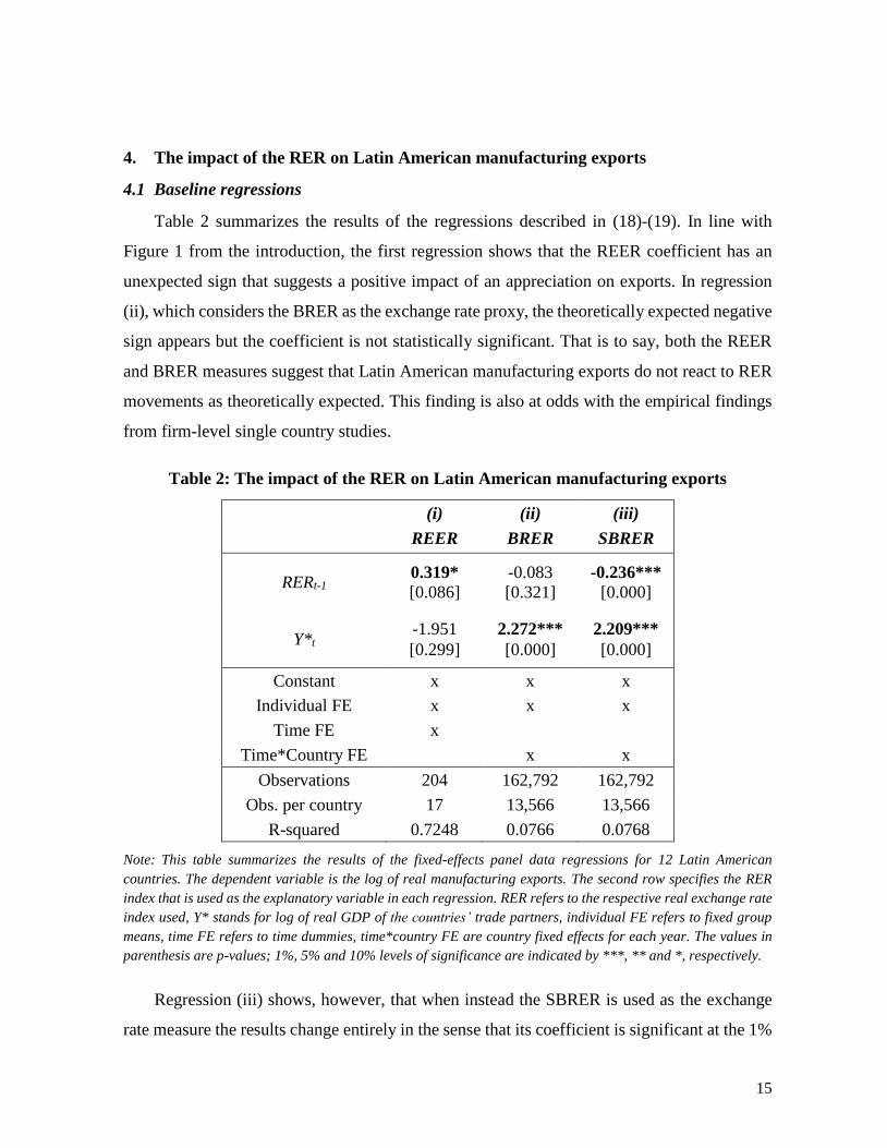
Table 2 summarizes the results of the regressions described in (18)-(19). In line with

Figure 1 from the introduction, the first regression shows that the REER coefficient has an

unexpected sign that suggests a positive impact of an appreciation on exports. In regression

(ii), which considers the BRER as the exchange rate proxy, the theoretically expected negative

sign appears but the coefficient is not statistically significant. That is to say, both the REER

and BRER measures suggest that Latin American manufacturing exports do not react to RER

movements as theoretically expected. This finding is also at odds with the empirical findings

from firm-level single country studies.

Table 2: The impact of the RER on Latin American manufacturing exports

(i) (ii) (iii)

REER BRER SBRER

RERt-1 0.319* -0.083 -0.236***

[0.086] [0.321] [0.000]

Y*t -1.951 2.272*** 2.209***

[0.299] [0.000] [0.000]

Constant x x x

Individual FE x x x

Time FE x

Time*Country FE x x

Observations 204 162,792 162,792

Obs. per country 17 13,566 13,566

R-squared 0.7248 0.0766 0.0768

Note: This table summarizes the results of the fixed-effects panel data regressions for 12 Latin American

countries. The dependent variable is the log of real manufacturing exports. The second row specifies the RER

index that is used as the explanatory variable in each regression. RER refers to the respective real exchange rate

index used, Y* stands for log of real GDP of the countries’ trade partners, individual FE refers to fixed group

means, time FE refers to time dummies, time*country FE are country fixed effects for each year. The values in

parenthesis are p-values; 1%, 5% and 10% levels of significance are indicated by ***, ** and *, respectively.

Regression (iii) shows, however, that when instead the SBRER is used as the exchange

rate measure the results change entirely in the sense that its coefficient is significant at the 1%

16

level. The coefficient value of 0.24 indicates that a 10% appreciation (depreciation) leads to a

2.4% decrease (increase) in manufacturing exports. This export elasticity is lower than those

reported in Torres García et al. (2018) for Colombia (value 0.77) and in Fornero et al. (2020)

for Chile (range 0.4; 0.6), for example, but, its value seems reasonable – especially considering

the above-mentioned weak reaction of the region’s manufacturing exports after the

depreciation of the mid-2010s.

Interestingly, in the aggregated REER regression external demand –measured as the

weighted average GDP of the trade partners– is not statistically significant and has an

unexpected negative sign (column 2). In the bilateral and sectoral export data regressions, on

the contrary, the predicted income elasticity is significant with the expected positive sign,

suggesting that a 10% increase in external income leads to an approximately 22% increase in

manufacturing exports (columns 3-4). Considering that the income elasticity is higher than the

SBRER elasticity, the results indicate that Latin American manufacturing exports are more

dependent on external income than on RER movements. This finding is in line with Fornero

et al.’s (2020) results for Chilean manufacturing exports. Most importantly for our purpose,

all of these results suggest that aggregated RER measures can lead to misleading results and

that it is important to account for sectoral heterogeneity when estimating export elasticities.

4.2 Robustness checks

The above presented baseline results might suffer from omitted variable bias (although

this is not very likely given that we control for individual and time specific effects). We

therefore consider the following covariates to check the robustness of the baseline results: an

interaction of the SBRER with the logarithm of sectoral manufacturing imports (in constant

USD), trade openness, domestic income and commodity prices. The first variable used is a

rough proxy for the impact that the integration of the manufacturing sector into global value

chains has on the RER export elasticity. A higher integration is expected to affect the elasticity

negatively, given that the change in the cost of imported inputs partly offsets the effects of

RER movements on foreign prices (Amiti et al., 2014; Ahmed et al., 2017). The import data

is obtained in the same way as the export data from above.

17

Trade openness, which is measured as the sum of total exports and imports as a fraction

of domestic GDP, is used as proxy for barriers to trade. It is common knowledge that exports

are negatively affected by trade barriers. Domestic GDP, on the other hand, is a proxy for

domestic demand and the potential of a country to adjust production to export demand. Finally,

commodity prices are used as a proxy for potential reallocation effects during commodity

booms and busts. According to Dutch Disease theory, changing commodity prices lead to the

reallocation of production factors between the manufacturing sector and the commodity and

service sector and thus affect manufacturing output (Corden & Neary, 1982). Trade openness

and domestic GDP data is available from the World Bank (2020), while the commodity price

data is retrieved from the IMF (2020).

Table 3: Robustness checks

(iv) (v) (vi) (vii)

SBRERt-1 -0.348*** -0.348*** -0.348*** -0.348***

[0.000] [0.000] [0.000] [0.000]

SBRERt-1 * Mt-1 0.009*** 0.009*** 0.009*** 0.009***

[0.000] [0.000] [0.000] [0.000]

Opennesst-1 78.777 23.029** -7.183

[0.120] [0.018] [0.422]

Yt-1 4.975 11.710*

[0.204] [0.076]

Commodity Pricest

-0.104*

[0.069]

Y*t 2.129*** 2.129*** 2.129*** 2.129***

[0.000] [0.000] [0.000] [0.000]

Observations 162,792 162,792 162,792 162,792

Obs. per country 13,566 13,566 13,566 13,566

R-squared 0.0778 0.0778 0.0778 0.0778

Note: This table summarizes the results of the fixed-effects panel data regressions for 12 Latin American

countries. All regressions include a constant, individual fixed effects and country fixed effects for each year. The

dependent variable is the log of real manufacturing exports. Please see Table 2 notes for more details.

Table 3 shows that the only variable that has a substantial impact on the baseline results

is the interaction of the SBRER with imports. The interaction term is highly significant and

18

positive in all regressions and, as expected, its addition increases the coefficient value of the

SBRER compared with the baseline results (-0.35 vs. -0.24). The interpretation of this result

is that a 10% increase in manufacturing imports diminishes the reaction of manufacturing

export to RER movements by 0.09%. This value is plausible in the sense that it is similar to

the one reported by Ahmed (2017, Table 2): When he interacts the REER with the country’s

participation in global value chains, the coefficient value is in the range 0.06 to 0.08. To put it

differently, these results indicate that when Latin American manufacturing exports have a low

(high) content of imported inputs, their average RER elasticity is slightly higher (lower) than

that reported in the baseline regression. Trade openness, domestic income and commodity

prices, on the other hand, are significant with the expected sign but they do not alter the

SBRER coefficient.

4.2 Sectoral RER export elasticities

The aggregated results from above might mask important differences across sectors.

According to theoretical models (Chen & Juvenal, 2016) and previous empirical findings

(Thorbecke & Smith, 2010; Torres García et al., 2018; Neumann & Tabrizy, 2021), the

responsiveness of exports to RER movements can differ substantially between sectors. One

important reason for this sectoral heterogeneity is that exports of low technology products tend

to respond more to RER movements, on the grounds that they can be substituted more easily

than more complex products and that they tend to have a lower cost share that is paid in the

currency of the destination country (because they rely more on local labor and less on imported

inputs and have lower distribution costs).

We thus make use of the disaggregated data at hand to explore the specific RER export

elasticity from each sector (𝛾0) by interacting the respective BRER and SBRER variable with

21 sector dummies (𝐷𝑠 = ∑ 𝐷𝑖3615 ):

𝑋𝑖𝑠𝑏𝑡 = 𝐷𝑠 ∗ 𝛾0𝑅𝐸𝑅𝑖𝑠𝑏𝑡−1 + 𝛽1𝑌𝑏𝑡∗ + 𝜔𝑖𝑡 + 𝜇𝑖𝑠𝑏 + 휀𝑖𝑠𝑏𝑡 (20)

19

Table 4: RER export elasticities by sector

(viii) (ix)

BRER SBRER

Food products & beverages (15) 0.144 -0.189

Tobacco products (16) -0.313 -0.563***

Textiles (17) -0.686*** -0.862***

Wearing apparel & fur dressing (18) -0.596** -0.754***

Leather dressing, footwear etc. (19) -0.737*** -0.687***

Wood & wood products etc. (20) -0.285 -0.414*

Paper and paper products (21) -0.374* -0.447**

Publishing & printing (22) -0.342* -0.495***

Chemicals & chemical products (24) 0.041 0.023

Rubber & plastics products (25) 0.147 0.113

Other non-metallic mineral products (26) -0.305 -0.452**

Basic metals (27) 1.141*** 0.793***

Fabricated metal products (28) 0.278 0.071

Machinery and equipment (29) -0.136 -0.196

Office & computing machinery (30) -0.161 -0.610***

Electrical machinery and apparatus (31) 0.284 -0.018

Radio, TV & communication equipment (32) -0.327 -0.476***

Medical, precision & optical instruments (33) 0.605** 0.662***

Motor vehicles (34) -0.200 -0.173

Other transport equipment (35) 0.204 0.252

Furniture & other manufacturing (36) -0.125 -0.269

Y*t 2.272*** 2.211***

Observations 162,792 162,792

Obs. per country 13,566 13,566

R-squared 0.0780 0.0784

Note: This table shows the RER elasticity of each manufacturing sector of the sample. All regressions include a

constant, individual fixed effects and country fixed effects for each year. The variable description of rows 3-23

(column 1) indicates the individual sector dummy that is multiplied by RER. Please see Table 2 notes for more

details.

The first observation from the results of this exercise, which are shown in Table 4, is that

more sectors react significantly to RER movements when the SBRER is used instead of the

BRER (12 vs. 7 sectors). The second observation is that, in line with the baseline regressions

in Table 2, the SBRER values are higher than those of the BRER. The third observation is that

20

the elasticities of the different sectors are distinct but their differences are not overly large:

The SBRER export elasticity ranges from 0.41 to 0.86 in the sectors that have significant

coefficients. Moreover, it is important to note that, as in the other regressions, the value of the

income elasticity is substantially higher than the individual RER elasticities, which suggests

that the exports from all sectors depend more on external income changes than on RER

movements.

Most importantly, and as expected, the results suggest that those sectors that are mainly

affected by SBRER movements are those that have a relatively low technological complexity

(i.e., tobacco, textiles, wearing apparel, leather dressing and footwear, and wood and paper

products). To verify econometrically if the RER elasticity of sectoral exports in Latin America

differs according to the technological sophistication of each sector, we use the following

regression:

𝑋𝑖𝑠𝑏𝑡 = 𝐷𝐿𝑀𝐻 ∗ 𝛿0𝑅𝐸𝑅𝑖𝑠𝑏𝑡−1 + 𝛽1𝑌𝑏𝑡∗ + 𝜔𝑖𝑡 + 𝜇𝑖𝑠𝑏 + 휀𝑖𝑠𝑏𝑡 (21)

where 𝐷𝐿𝑀𝐻 = ∑ 𝐷𝑗31 is a dummy variable that accounts for the average technological

sophistication of low-, medium- and high-technology sector groups (𝛿0).

The technological complexity of each sector is approximated by its average Product

Complexity Index (PCI)9 value from the year 2018. PCI values are available from the Atlas of

Economic Complexity (2020) at a three-digit HS4 level. Using the HS Combined to ISIC Rev

3 concordance table from WITS (2020a), we construct a PCI value for each sector by

averaging the PCI values of all products that comprise the respective sector. The seven sectors

that have the highest PCI value are categorized in the high-technology sector group (Group H;

values >0.50), the seven sectors with the lowest PCI value form the low-technology sector

group (Group L; <0.15) and the remaining seven sectors are classified as the medium-

technology sector group (Group M).10

9 The PCI “ranks the diversity and sophistication of the productive know-how required to produce a product.

Products with a high PCI value (the most complex products that only a few countries can produce) include

electronics and chemicals. Products with a low PCI value (the least complex product that nearly all countries can

produce) include raw materials and simple agricultural products” (Atlas of Economic Complexity, 2020). 10 The average PCI values for each sector are the following: 18=-1.02; 15=-0.76; 19=-0.70; 16=-0.68; 20=-0.66;

17=-0.31; 36=0.01; 35=0.16; 27=0.26; 26=0.29; 21=0.38; 22=0.39; 25=0.43; 24=0.44; 28=0.50; 34=0.69;

32=0.77; 31=0.78; 30=0.84; 33=0.89; 29=0.96.

21

Table 5 indicates that RER movements indeed seem to affect mainly exports from low

technology sectors in Latin America. While the BRER and the SBRER are significant at the

1%-level in the low-technology group, both are not significant in the medium- and high-

technology sector groups. As discussed above, the result that RER movements mainly affect

low technology sectors is in line with previous literature. Having said that, the results obtained

from the two measure differs insofar that the coefficient size of the SBRER is nearly 50%

larger than that of the BRER. To be more precise, the SBRER coefficient indicates that low

technology sectors in Latin America have a RER export elasticity of 0.55 (i.e. a 10%

depreciation leads to a 5.5% increase in exports).

Table 5: RER export elasticities according to sectoral complexity

(x) (xi)

BRER SBRER

Low-technology -0.371*** -0.548***

[0.000] [0.000]

Medium-technology 0.073 -0.038

[0.502] [0.690]

High-technology 0.049 -0.134

[0.648] [0.124]

Y*t 2.272*** 2.214***

[0.000] [0.000]

Observations 162,792 162,792

Obs. per country 13,566 13,566

R-squared 0.0769 0.0772

Note: This table shows the RER elasticity of sector groups according to their technological complexity. All

regressions include a constant, individual fixed effects and country fixed effects for each year. The variables

low-, medium- and high-technology are sector dummies that are multiplied by the respective RER measure.

Please see Table 2 notes for more details.

In general, all regression results show that the SBRER measure tends to reveal higher

elasticities than the BRER measure. This finding is in accordance with the diverging RER

elasticities that are reported by studies that use aggregate data versus those that use

disaggregate data (i.e. firm-level studies tend to report higher RER elasticities than aggregate

data studies). Most importantly, only the SBRER measure is significant in the baseline

22

regression. Overall, these results indicate that it is important to consider cross sectoral

distinctions regarding trade partners and production costs when estimating RER export

elasticities at an aggregate level.

5. Conclusions

In this paper we have exploited the variations across manufacturing sectors to determine

the importance of RER movements for Latin American manufacturing exports during 2001-

2018. Our main finding is that it is important to account for cross-sector variations. The

baseline regressions that use the REER and BRER as exchange rate measure show results that

are contrary to the predictions of standard trade theories. When instead a measure is used that

considers sectoral differences in terms of trade partners and cost evolutions (the SBRER),

RER movements become a significant determinant of aggregate manufacturing exports with

the expected sign. Moreover, the results indicate that the RER elasticities of exports from

individual sectors and sector groups are distinct, and that the more refined SBRER is better

suited than the BRER to reveal these distinctions. More specifically, in the Latin American

case mainly low-technology exports are affected by RER movements.

These findings indicate that strong RER appreciations, for example due to positive

commodity shocks, mainly limit the export growth of the regions labor-intensive

manufacturing sectors, and thus only give partial support to the “New Developmentalist” view

that a competitive RER can be seen as effective policy tool that fosters economic growth.

When Latin American countries engage in exchange rate management, they have to be aware

that this policy will affect individual sectors in distinct ways and will have only limited

benefits for technologically complex sectors. To put it differently, the results indicate that the

development of competitive high-technology sectors in Latin America rather requires

industrial policies than exchange rate management.

These insights can also help policy makers to better identify if the potential benefits of

establishing competitive RER outweigh the associated costs (such as increasing import prices

and declining real wages). Considering the existing trade-offs, recent research recommends

establishing a system of multiple effective exchange rates to target specific sectors (Guzman

23

et al, 2018). While the implementation of multiple exchange rates seems challenging in

practice, our findings might be helpful for countries that wish to implement such a policy.

Having said this, for policy purposes it would be important that future research

corroborates our findings on a country level, given that our cross-country setting might

obscure important distinctions between countries. Finally, it is important to note that the

obtained results indicate that external demand is more important for the growth of Latin

American manufacturing exports than RER movements. Hence, policy makers of the region

should increase their efforts to develop strategies that enable firms to export to the largest

economies in the world, given that these countries have large market potential.

References

Ahmed, S., Appendino, M. & Ruta, M. (2017). Global value chains and the exchange rate

elasticity of exports. The B.E. Journal of Macroeconomics, 17(1): 1-24.

Amiti, M., Itskhoki, O. & Konings, J. (2014). Importers, Exporters, and Exchange Rate

Disconnect. American Economic Review, 104(7): 1942-1978.

Atlas of Economic Complexity (2020). “Country & Product Complexity Rankings”. Retrieved

from https://atlas.cid.harvard.edu/rankings/product.

Bhattacharya, P.S., Karayalcin, C.A.; & Thomakos, D.D. (2008). Exchange rate pass-through

and relative prices: An industry-level empirical investigation. Journal of International

Money and Finance, 27(7): 1135-1160

Berka, M., Devereux, MB., & Engel, C. (2018). Real Exchange Rates and Sectoral

Productivity in the Eurozone. American Economic Review, 108(6), 1543-1581.

Berman, N., Martin, P. & Mayer, T. (2012). How do Different Exporters React to Exchange

Rate Changes? Quarterly Journal of Economics, 127(1): 437-492.

BIS (2020). “Statistics – Foreign Exchange”. Retrieved from https://www.bis.org/

statistics/index.htm.

Bresser-Pereira, L.C. (2016). Reflecting on new developmentalism and classical

developmentalism. Review of Keynesian Economics, 4(3): 331-352.

Bresser-Pereira, L.C., and Rugitsky, F. (2018). Industrial policy and exchange rate scepticism?

Cambridge Journal of Economics, 42(3): 617-632.

Bresser-Pereira, L.C. (2020). Neutralizing the Dutch disease. Journal of Post Keynesian

Economics, 43(2): 298-316.

24

Bresser-Pereira, L.C. (2020a). New Developmentalism: Development macroeconomics for

middle-income countries. Cambridge Journal of Economics, 44(3): 629-646.

Byrne, J.P, Darby, J. & MacDonald, R. (2008). US trade and exchange rate volatility: A real

sectoral bilateral analysis. Journal of Macroeconomics, 30: 238-259.

Campa, J.M. & Goldberg, L.S. (2005) Exchange Rate Pass-Through into Import Prices.

Review of Economics and Statistics, 87: 679-90.

Carvalho, C. & Nechio, F. (2011). Aggregation and the PPP Puzzle in a Sticky-Price Model.

American Economic Review, 101(6): 2391-2424.

Casas, C. (2020). Industry heterogeneity and exchange rate pass-through. Journal of

International Money and Finance, 106: 1-20.

Chen, N. & Juvenal, L. (2016). Quality, trade, and exchange rate pass-through. Journal of

International Economics, 100: 61-80.

Cheung, Y.-W. & Sengupta (2013). Impact of exchange rate movements on exports: An

analysis of Indian non-financial sector firms. Journal of International Money and Finance,

39: 231-245.

Corden, W. M., & Neary, J. P. (1982). Booming sector and de-industrialisation in a small open

economy. The Economic Journal, 92(368): 825-848.

Dai, M. & Xu, J. (2013). Industry-specific Real Effective Exchange Rate for China: 2000-

2009. China & World Economy, 21(5): 100-120.

Dai, M., Nucci, F., Pozzolo, A.F. & Xu, J. (2021). Access to finance and the exchange rate

elasticity of exports. Journal of International Money and Finance, 115: 1-23.

Fang, W.S., Lai, Y.H. & Miller, S.M. (2006). Export Promotion through Exchange Rate

Depreciation or Stabilization? Southern Economic Journal, 72(3): 611-626.

Fornero, J.A., Fuentes, M.A., Sangama, A.G. (2019). How do manufacturing exports react to

the real exchange rate and foreign demand? The Chilean case. World Economy, 43(1): 274-

300.

Goldberg, L.S. (2004). Industry-specific exchange rates for the United States. FRBNY

Economic Policy Review, 10(1): 1-16.

Greenaway, D., Kneller, R. & Zhang, X. (2010). The Effect of Exchange Rates on Firm

Exports: The Role of Imported Intermediate Input. World Economy, 33(8): 961-986.

Guzman, M., Ocampo, J.A. & Stiglitz, J.E. (2018). Real exchange rate policies for economic

development. World Development, 110: 51-62.

Imbs, J., Mumtaz, H., Ravn, M.O. & Rey, H. (2005). PPP Strikes Back: Aggregation and the

Real Exchange Rate. Quarterly Journal of Economics, 120(1): 1-43.

25

IMF (2015). Exchange Rates and Trade Flows: Disconnected?. In IMF (eds.): World

Economic Outlook, October 2015. Washington, D.C.: International Monetary Fund, Chapter

3.

IMF (2020). “Commodity Terms of Trade - IMF Data”. Retrieved from https://data.imf.org/

?sk=2CDDCCB8-0B59-43E9-B6A0-59210D5605D2.

Kang, J.W. & Dagli, S. (2018). International Trade and Exchange Rates. Journal of Applied

Economics, 21(1): 84-105.

Lee, J. & Yi, B. (2005). “Industry level real effective exchange rates for Korea. Institute for

Monetary and Economic Research”. The Bank of Korea.

Li, H., Ma, H. & Xu, Y. (2015). How do exchange rate movements affect Chinese exports? –

A firm-level investigation. Journal of International Economics, 97: 148-161.

Mayer, T. & Steingress, W. (2020). Estimating the effect of exchange rate changes on total

exports. Journal of International Money and Finance, 106: 1-22.

Mayoral, L. & Gadea, M.D. (2011). Aggregate real exchange rate persistence through the lens

of sectoral data. Journal of Monetary Economics, 58: 290-304.

Neumann, R. & Tabrizy, S.S. (2021). Exchange Rates and Trade Balances: Effects of Intra-

Industry Trade and Vertical Specialization. Open Economics Review,

doi.org/10.1007/s11079-020-09612-4.

Ocampo, J.A. (2017). Commodity-Led Development in Latin America. International

Development Policy, 9: 51-76.

Reinhart, C. (1995). Devaluation, Relative Prices and International Trade. IMF Staff Papers,

42(2): 290-312.

Robertson, R., Kumar, A. Dutkowsky, D.H. (2009). Purchasing Power Parity and aggregation

bias for a developing country: The case of Mexico. Journal of Development Studies, 90(2):

237-243.

Saygili, H. & Saygili, M. (2019). Exchange rate pass-through into industry specific prices: An

analysis with industry-specific exchange rates. Macroeconomic Dynamics, 25(2): 304-336.

Sato, K., Junko, S., Shrestha, N. & Zhang, S. (2013). Industry-specific Real Effective

Exchange Rates and Export Price Competitiveness: The Cases of Japan, China, and Korea.

Asian Economic Policy Review, 8: 298-321.

Sekkat, K. & Varoudakis, A. (2000). Exchange rate management and manufactured exports

in Sub-Saharan Africa. Journal of Development Economics, 61: 237-253.

Tang, H. & Zhang, Y. (2012). Exchange Rates and the Margins of Trade: Evidence from

Chinese Exporters. CESifo Economic Studies, 58(4): 671-702.

26

Thorbecke, W. & Smith, G. (2010). How Would an Appreciation of the Renminbi and Other

East Asian Currencies Affect China’s Exports? Review of International Economics, 18(1):

95-108.

Torres García, A., Goda, T. & Sánchez González, S. (2018). Efectos diferenciales de la tasa

de cambio real sobre el comercio manufacturero en Colombia. Ensayos sobre Política

Económica, 36(86): 193-206.

WITS (2020a). “Product Concordance”. Retrieved from https://wits.worldbank.org/

product_concordance.html.

WITS (2020b). “Trade Data – UN Comtrade”. Retrieved from https://wits.worldbank.org.

World Bank (2020). “World Development Indicators”. Retrieved from

https://databank.worldbank.org/source/world-development-indicators.

27

APPENDIX

Table A1: Overview of the PPI Data used for the calculation of the SBRER

ISO3 Used Price Index Start End Divisions w/o Data Source Note

ARG PPI-by division 2001 2018 30 Office for National Statistics (INDEC) Missing division imputed with aggregate man. PPI

BEL PPI-by division 2010 2018 Belgian statistical office (Statbel) 2001-2009 two-dig-level data imputed with IFS' PPI

growth rate PPI-all commodities 2001 2009 International Financial Statistics (IFS)

BOL PPI-by division 2001 2014 20,22,26,29-35 Office for National Statistics (INE) Missing divisions imputed with aggregate man. PPI;

2015-2018 imputed with IFS' CPI growth rate CPI 2015 2018 International Financial Statistics (IFS)

BRA PPI-by division 2009 2018 Office for National Statistics (IBGE) 2001-2008 two-dig-level data imputed with growth rate

of IFS' PPI-AC PPI-all commodities 2001 2008 International Financial Statistics (IFS)

CAN PPI-by division 2001 2018 28,32 Statistics Canada (StatCan) Missing divisions imputed with aggregate man. PPI

CHE PPI-by division 2004 2018 Federal Statistical Office Switzerland 2001-2004 two-dig-level data imputed with IFS' PPI

growth rate PPI-all commodities 2001 2004 International Financial Statistics (IFS)

CHL PPI-by division 2007 2018

Office for National Statistics (INE) 2001-2006 two-dig-level data imputed with aggregate

man. PPI PPI aggregate manuf. 2001 2006

CHN PPI-by division 2012 2018 National Bureau of Statistics 2001-2011 two-dig-level data imputed with IFS' PPI

growth rate PPI-all commodities 2001 2011 International Financial Statistics (IFS)

COL PPI-by division 2006 2018

Office for National Statistics (DANE) 2001-2005 two-dig-level data imputed with IFS' PPI

growth rate PPI aggregate manuf. 2001 2005

CRI PPI-by division 2012 2018 16 Central Bank of Costa Rica 2001-2011 two-dig-level data imputed with IFS' PPI

growth rate PPI-all commodities 2001 2011 International Financial Statistics (IFS)

DEU PPI-by division 2009 2018 Federal Statistical Office Germany 2001-2008 two-dig-level data imputed with IFS' PPI

growth rate PPI-all commodities 2001 2008 International Financial Statistics (IFS)

DOM PPI-by division 2013 2018 32 Office for National Statistics (ONE) Missing division imputed with aggregate man. PPI;

2001-2012 imputed with CPI growth rate CPI 2001 2012 Banco Central de Rep. Dominicana

ECU PPI-by division 2001 2018 32 Office for National Statistics (INEC) Missing division imputed with aggregate man. PPI

ESP PPI-by division 2001 2018 Instituto Nacional de Estadística (INE)

FRA PPI-by division 2001 2018 16 Office for National Statistics (INSEE) Missing division imputed with aggregate man. PPI

GBR PPI-by division 2001 2018 Office for National Statistics (ONS)

GTM CPI 2010 2018 all Central Bank of Guatemala Two-dig-level data imputed with CPI

28

HKG PPI-by division 2005 2018 19,20,23-25,28-36 Census and Statistics Department Missing divisions imputed with aggregate man. PPI;

2001-2004 imputed with CPI growth rate CPI 2001 2004 International Financial Statistics (IFS)

HND CPI 2001 2018 all International Financial Statistics (IFS) Two-dig-level data imputed with CPI

IDN PPI aggregate manuf. 2010 2018 Badan Pusat Statistik Two-dig-level data imputed with aggregate man. PPI &

wholesale price data Wholesale price index 2001 2009 World Bank

IND Manufacturing PPI 2001 2018 all Central Bank of India Two-dig-level data imputed with aggregate man. PPI

ITA PPI-by division 2001 2018 16 National Institute of Statistics Missing division imputed with aggregate man. PPI

JPN PPI-by division 2001 2018 16,19,22,33-34 Central Bank of Japan Missing divisions imputed with aggregate man. PPI

KOR PPI-by division 2001 2018 16,22,25,30-32,34,36 Central Bank of Korea Missing divisions imputed with aggregate man. PPI

MEX PPI-by division 2001 2018 21 Office for National Statistics (INEGI) Missing division imputed with aggregate man. PPI

MYS PPI-by division 2001 2016 16-22,25,27,28,30,32,34,36 Department of Statistics Missing divisions imputed with aggregate man. PPI;

2017-2018 imputed with IFS' PPI growth rate PPI-all commodities 2017 2018 International Financial Statistics (IFS)

NIC PPI-by division 2006 2018 30,32 Central Bank of Nicaragua Missing divisions imputed with aggregate man. PPI;

2001-2005 imputed with CPI growth rate CPI 2001 2005 International Financial Statistics (IFS)

NLD PPI-by division 2012 2018 Statistics Netherlands 2001-2011 two-dig-level data imputed with IFS' PPI

growth rate PPI-all commodities 2001 2011 International Financial Statistics (IFS)

PAN PPI-by division 2016 2018 16, 23, 30 & 32 Office for National Statistics (INEC) Missing divisions imputed with aggregate man. PPI;

2001-2015 imputed with WPI growth rate Wholesale price index 2001 2015 World Bank

PER Manufacturing PPI 2001 2018 15-36 Office for National Statistics (INEI) Missing division imputed with aggregate man. PPI

PRY PPI-all commodities 2001 2018 all International Financial Statistics (IFS) Two-dig-level data imputed with aggregate man. PPI

RUS PPI aggregate manuf. 2001 2018 all Federal State Statistic Service Two-dig-level data imputed with aggregate man. PPI

SWE PPI-by division 2001 2018 Statistics Sweden

SGP PPI-by division 2001 2018 Departament of Statistics

SLV Manufacturing PPI 2010 2017 15-36 Office for National Statistics Missing divisions imputed with aggregate man. PPI;

2001-2009 & 2018 imputed with IFS' PPI growth rate PPI-all commodities 2001 2018 International Financial Statistics (IFS)

THA PPI-by division 2001 2018 36 Trade Policy and Strategy Office (TPSO) Missing division imputed with aggregate man. PPI

URY PPI-by division 2001 2018 29, 30, 32-33 Office for National Statistics Missing division imputed with aggregate man. PPI

USA PPI-by division 2001 2018 Bureau of Labor Statistics

VNM PPI-by division 2009 2018 32 Missing divisions imputed with aggregate man. PPI;

2001-2008 data imputed with aggregate man. PPI PPI aggregate manuf. 2001 2008 General Statistics Office of Vietnam

Note: This table gives an overview of the used price indices and their data sources and describes any imputations that were necessary to have data for all years

and sectors. The columns’ start and end indicate the years for which the specific data is available.

29

Table A2: Concordance tables used to homogenize the PPI data

From To Country Source

ISIC Rev. 4

NACE Rev. 2 ISIC Rev. 3

BEL, BRA, CHE, CRI,

DEU, DOM, ECU, ESP,

FRA, ITA, MYS, NLD,

SWE, SGP, THA, VNM

United Nation Statistics Division

NAICS 2017 ISIC Rev. 4 CAN, USA United States Census Bureau

CPA Rev. 2.1 ISIC Rev. 4 GBR United Nation Statistics Division

HSIC V2.0 ISIC Rev. 4 HKG United Nation Statistics Division

KSIC ISIC Rev. 4 KOR Korean Standard Statistical

Classification

SCIAN 2013 ISIC Rev. 4 MEX Instituto Nacional de Estadística y

Geografía (INEGI)

JSIC Rev. 12 NACE Rev. 2 JPN EuroStat - RAMON

Note: This table lists the concordance tables used to homogenize the PPI data. If one ISIC Rev. 3 division is equal to

various divisions from the source nomenclature, the data are averaged (e.g., when transforming from ISIC Rev. 4 to

Rev. 3, the PPI from division 15 is the average PPI from divisions 10-11 and 20 of Rev. 4).

Table A3: Phillips–Perron panel data unit root test statistics

P Z L* Pm

𝑿𝒔𝒃𝒕 62,600 -125.3 -156.9 222.2

(0.00) (0.00) (0.00) (0.00)

𝑺𝑩𝑹𝑬𝑹𝒔𝒃𝒕 23,300 -1.80 -7.97 20.98

(0.00) (0.04) (0.00) (0.00)

with demean option

𝑿𝒔𝒃𝒕 70,400 -141.8 -175.7 261.9

(0.00) (0.00) (0.00) (0.00)

𝑺𝑩𝑹𝑬𝑹𝒔𝒃𝒕 24,600 -6.59 -12.3 28.0

(0.00) (0.00) (0.00) (0.00)

with time trend option

𝑿𝒔𝒃𝒕 61,700 -117.0 -150.1 217.2

(0.00) (0.00) (0.00) (0.00)

𝑺𝑩𝑹𝑬𝑹𝒔𝒃𝒕 34,700 -34.6 -45.1 79.4

(0.00) (0.00) (0.00) (0.00)

Note: This table shows the results of Fisher-type Phillips–Perron unit-root tests on X and SBRER (specifying one lag in

the Stata command). With one exception, all tests reject the null hypothesis that all panels contain unit roots at the 1%-

level (the respective p-values are listed in brackets).