Section Notes 2

Introduction to optimization and linear optimization

Applied Math 121

Week of February 7, 2011

Goals for the week

1. be able to put any LP into canonical form.

2. understand the relationship between basic solutions and extreme points.

3. know what non-linear programs can be transformed into linear programs and how to do so.

4. be comfortable with basic AMPL syntax relevant to defining LPs.

Contents

1 The Objective Function and Solutions for LPs 2

2 The Standard Form and the Canonical Form 3

3 Basis, Variables, Extreme Points and Solutions 6

3.1 Review . . . . . . . . . . . . . . . . . . . . . . . . . . . . . . . . . . . . . . . . . . . . 63.2 Finding Basic, Feasible Solutions and Extreme Points . . . . . . . . . . . . . . . . . 73.3 Learning to pivot . . . . . . . . . . . . . . . . . . . . . . . . . . . . . . . . . . . . . . 8

4 Making non-linear functions linear 9

5 Modelling with AMPL - The Street Illumination Problem 10

5.1 Optimal Street Illumination Problem . . . . . . . . . . . . . . . . . . . . . . . . . . . 105.2 A Review of AMPL syntax . . . . . . . . . . . . . . . . . . . . . . . . . . . . . . . . 125.3 The Production Model in AMPL . . . . . . . . . . . . . . . . . . . . . . . . . . . . . 135.4 Street Illumination, in AMPL . . . . . . . . . . . . . . . . . . . . . . . . . . . . . . . 145.5 A Review of Set Notation . . . . . . . . . . . . . . . . . . . . . . . . . . . . . . . . . 16

6 Solutions 18

1

1 The Objective Function and Solutions for LPs

Consider the following linear program:

maximize c1x1 + c2x2

subject to x2 ≥ 1

x1 + x2 ≥ 2

for nonzero constants c1 and c2.

Exercise 1

Can you find an example of values for c1 and c2 such that the problem

1. has a single optimal solution?

2. has exactly two optimal solutions?

3. has an infinite number of optimal solutions.

4. becomes infeasible?

End Exercise 1

By completing the above exercises, you should now:

• understand the relationship between the objective function, constraints, fea-sibility, and the number of optimal solutions.

• be comfortable identifying coefficients that will change the number of optimalsolutions.

2

K10 K5 0 5 10

K5

5

10

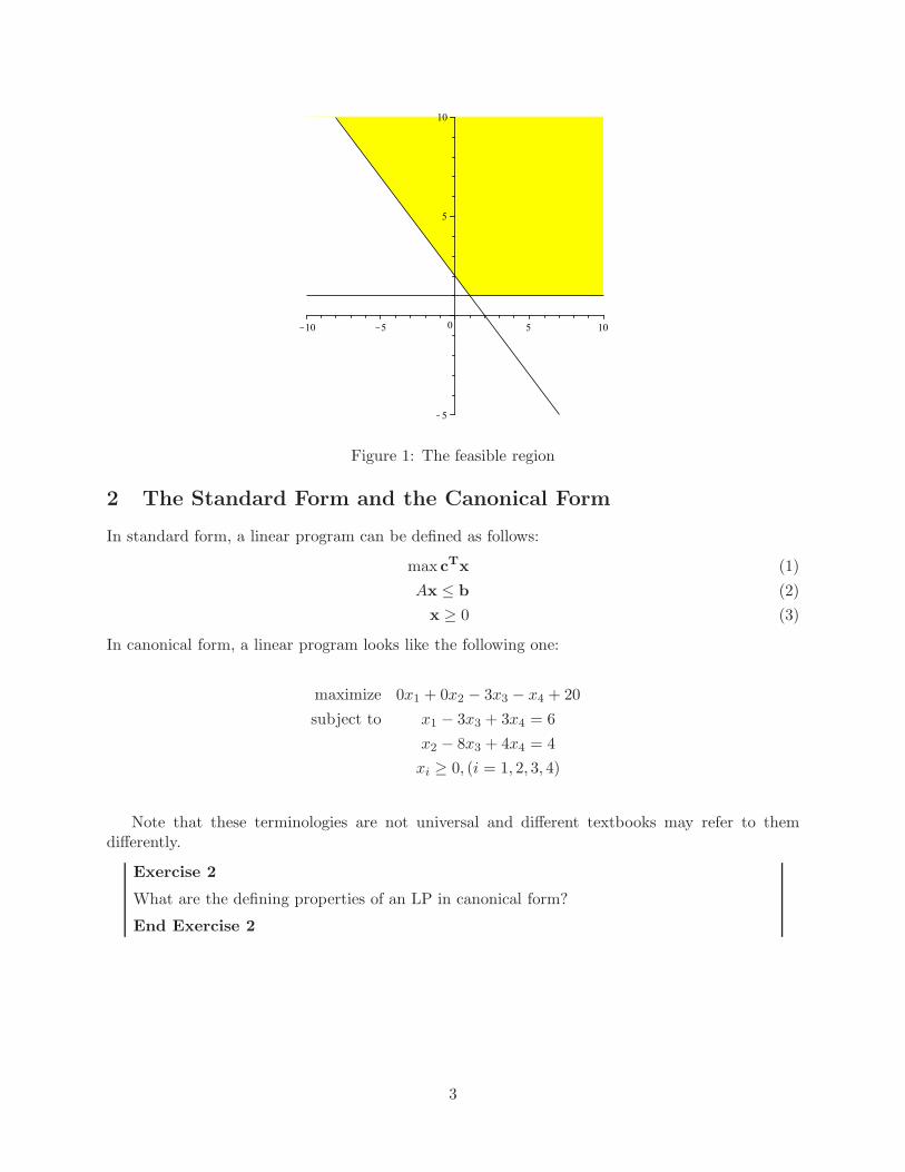
Figure 1: The feasible region

2 The Standard Form and the Canonical Form

In standard form, a linear program can be defined as follows:

max cTx (1)

Ax ≤ b (2)

x ≥ 0 (3)

In canonical form, a linear program looks like the following one:

maximize 0x1 + 0x2 − 3x3 − x4 + 20

subject to x1 − 3x3 + 3x4 = 6

x2 − 8x3 + 4x4 = 4

xi ≥ 0, (i = 1, 2, 3, 4)

Note that these terminologies are not universal and different textbooks may refer to themdifferently.

Exercise 2

What are the defining properties of an LP in canonical form?

End Exercise 2

3

Exercise 3

Is the canonical form restrictive in any way?

End Exercise 3

4

Exercise 4

What are the advantages of having an LP in canonical form?

End Exercise 4

Exercise 5

Convert the following LP to canonical form:

minimize x1 + 3x2

subject to 2x1 + x2 ≥ −5

x1 − x2 ≤ 6

xi ≥ 0, (i = 1, 2)

End Exercise 5

By completing the above exercises, you should now:

• know the definition and properties of canonical form.

• be able to put any LP into canonical form.

5

3 Basis, Variables, Extreme Points and Solutions

3.1 Review

Linear algebra review:

1. A basis of Rm is a set of linearly independent m-dimensional vectors v1, ..., vm with theproperty that every vector of Rm can be written as a linear combination of the vectorsv1, ..., vm. Note that the vectors v1, ..., vm form a square matrix that is invertible. Thesevectors v1, ..., vm span the vector space Rm.

2. A basis B for an arbitrary m-by-n matrix A can also be seen as a list of m numbers chosenfrom {1, 2,. . . , n} such that the square matrix AB with m columns from A indexed by this listis a basis for Rm, i.e. the column vectors span the space Rm. Again, AB will be invertible.

Basic feasible solutions and extreme points

1. Basic variables for a given basis B are the ones corresponding to the column vectors of B.

2. Non-basic variables for a given basis B are all variables except the basic variables.

3. The basic solution x of the system Ax = b for a basis B is the unique solution of this systemwhere all non-basic variables are equal to zero (xj = 0 for all indices j 6∈ B).

4. A feasible solution is a solution for an LP which satisfies all the constraints.

5. A basic feasible solution is a solution for an LP that is both basic and feasible. Note thatbasic solutions for LPs in canonical form are solutions for Ax = b but they might be infeasibleif the non-negativity requirements for the decision variables are not satisfied.

6. Let S be the set of points in the feasible region of an LP. A point y in S is called an extreme

point of S if y cannot be written as y = λw + (1 − λ)x for two distinct point w and x in S

and 0 < λ < 1. That is, y does not lie on the line segment joining any two points of S.

7. Every basic feasible solution of an LP corresponds to an extreme point of the feasibleregion of the LP.

6

3.2 Finding Basic, Feasible Solutions and Extreme Points

Example: Consider the following two constraints:

x1 + x2 = 2

2x1 + 2x2 = 3

Exercise 6

Can we find a vector (x1, x2) that satisfies both constraints, i.e. a basic solution?

End Exercise 6

Now, consider the set of vectors x satisfying the following constraints:

x1 + 2x2 + 2x3 = 4

2x1 + 4x2 + 3x3 = 7

x1, x2, x3 ≥ 0

Exercise 7

1. List the basic solutions corresponding to these equations. For each basic solutionyou write down, specify the columns of the coefficient matrix corresponding to thesolution. Which ones are feasible?

2. Find an extreme point of the feasible region.

3. Find a feasible solution that is not an extreme point.

End Exercise 7

7

By completing the above exercises, you should now:

• understand the relationship between basic solutions and extreme points.

• know how to obtain all basic solutions for a given LP by putting it into canon-ical form.

3.3 Learning to pivot

The Simplex algorithm iterates from tableau to tableau by performing pivot operations. In thefollowing exercise, we will get some practice with pivoting. But first two more definitions beforewe start:

• Let ek be the m-dimensional unit column vector (0, . . . , 1, . . . , 0) with a 1 in the k-th placeand 0’s elsewhere. The m-by-n matrix A is in canonical form if all the vectors ek occuras columns of A.1

• Pivoting is the process of applying algebraic manipulations (multiplying rows with scalars,adding rows to other rows) to a matrix such that we get one in canonical form. One pivot

operation refers to the series of algebraic manipulations to get one new unit vector ek in thematrix that wasn’t there before.

Now, consider the following matrix:

(

1 2 32 3 4

)

Exercise 8

1. Using 2 pivot operations, arrive at a tableau matrix in canonical form.

2. Using the matrix found in the previous exercise, find one other corresponding matrixin canonical form by using a single pivot operation.

End Exercise 8

1Except that ek need not occur if the k-th row of A is zero. You can think about when this may occur in a linear

program.

8

By completing the above exercises, you should now:

• know how to use pivot operations to arrive at a tableau in canonical form.

• know how to use pivots to bring in a new unit vector.

4 Making non-linear functions linear

In practice, non-linear objective functions appear quite frequently. Solving a non-linear programis generally far more difficult than a linear program. Sometimes non-linear functions are approxi-mated using linear functions and solved, but this approximation is very inaccurate. Occasionally, anonlinear program can be transformed into a linear program (without any loss of accuracy). Whilethis is rare, it can be useful.

Determining when a non-linear objective function can be linearized.

1. The maximum of several linear functions is convex.

2. A function f(x) is a friendly non-linear function if it can be written as the maximum of oneor more linear functions.

3. An objective function for a minimization problem is friendly if it is a friendly non-linearfunction or the sum of friendly non-linear functions.

4. If a minimization problem has a friendly objective function its feasible region is that of anLP and the problem can be expressed as a linear program.

Exercise 9

Why does a friendly objective function for a minimization problem guarantee that thefeasible region can be represented using an LP? (hint: Think about this what this meansgraphically)

End Exercise 9

Exercise 10

Does the above hold for a maximization problem? Why or why not?

End Exercise 10

9

Exercise 11

Transform the following non-linear program into an L.P.

minimize | x1 | + | x2 | + | x3 | + | x4 | + | x5 | + | x6 | + | x7 |

subject to x1 + x4 + x7 ≥ 5

x1 + x2 + x3 + x6 ≥ 8

Hint: Consider the graph | x1 | and determine how the maximum of two or more linearfunctions could generate the same graph.

End Exercise 11

By completing the above exercises, you should now:

• have an idea what non-linear programs can be transformed into linear pro-grams without a lose of accuracy.

• be able to linearize a non-linear program by introducing variables and con-straints to minimization problems with friendly objective functions.

5 Modelling with AMPL - The Street Illumination Problem

5.1 Optimal Street Illumination Problem

Suppose we have a street that is five units long. At each unit, there is a lamp post with a dimmablelamp (i.e. we can control the power used and thus light generated at each post). At each of the threemiddle units of the street there is a store, and these stores have minimum lighting requirements of5, 3 and 7 respectively. Each street light casts a beam over its own area of the street, as well asthe areas to each side in a proportion of 10%, 80%, 10% of the total light produced by the lampburning at a specific intensity. Your goal: light the street by at least as much as is required by thestore owners, while using as little power as possible.

10

Given this setup, lets use the techniques we have gone over to make an elegant model for thisproblem:

Exercise 12

1. What are the sets implicit in the problem?

2. What are the decision variables?

3. What is the objective function?

4. What are the constraints? Hint: Think about how can we use offset indexing toelegantly describe the constraints

5. What if instead of wanting to minimize the total power used, the store owners wantedto minimize the difference between the required power and the power received? Giveall the relevant changes to the LP if the goal is to minimize the absolute differencebetween the power required and the power received.

End Exercise 12

11

5.2 A Review of AMPL syntax

As part of your current problem set, you will need to be able to create matrices of both variablesand parameters in your AMPL code.

Exercise 13

1. What is the syntax for declaring a parameter?

2. What is the syntax for declaring a vector of parameters?

3. What is the syntax for declaring a matrix of parameters?

4. What is the syntax for declaring a variable?

5. What is the syntax for declaring a vector of variables?

6. What is the syntax for declaring a matrix of variables?

7. What is the syntax for defining a parameter?

8. What is the syntax for defining a vector of parameters?

9. What is the syntax for defining a matrix of parameters?

End Exercise 13

By completing the above exercises, you should now:

• be comfortable with basic AMPL syntax relevant to defining LPs.

12

5.3 The Production Model in AMPL

In this example we have a set of products that use up resources to manufacture and store. Specifi-cally the resources are machine time and storage space. Each product fetches a certain profit perunit sold. The producer wants to maximize profit. Let us formulate the model:

Sets P set of product types

R set of resources

Parameters ai, i ∈ R amount of resource i available

pj , j ∈ P per unit profit for product j

uij , i ∈ R, j ∈ P amount of resource i required per unit production of j

Variables xj , j ∈ P quantity of product j to produce

max∑

j∈P

pjxj maximize total profit

s.t.∑

i∈R uijxj ≤ aj ∀i ∈ R resource constraints

We are given the following data. There are 2 products A and B. Product A earns a profit of 5per unit sold, and uses 1 unit of machine time and 5 units of storage space. Product B earns aprofit of 8 per unit sold, and uses 1 unit of machine time and 9 units of storage space. The totalmachine time available is 6 and the total storage space is 45. Using this data to fill in the sets andparameters we have defined we get: P = {A,B}, R = {machine, space}, a = {6, 45}, p = {5, 8},umachine = {1, 1}, uspace = {5, 9}. Here we have assumed that the parameter values over sets areordered according to the order of the elements appearing in the set (e.g. A before B). We can thenwrite the linear program as follows:

max 5x1 + 8x2

s.t. : x1 + x2 ≤ 6

5x1 + 9x2 ≤ 45

xi ≥ 0, (i = 1, 2)

Exercise 14

What would the example model and data files look like in AMPL?

End Exercise 14

13

File: example.mod

set PRODUCT;

set RESOURCE;

param usage {i in RESOURCE, j in PRODUCT};

param profit {j in PRODUCT};

param avail {i in RESOURCE};

var X {j in PRODUCT}>=0;

maximize Total_Profit: sum {j in PRODUCT} profit[j]*X[j];

subject to Resource_Constraints {i in RESOURCE}: sum{j in PRODUCT}

usage[i, j]*X[j]<=avail[i];

File: example.dat

set PRODUCT := A B;

set RESOURCE := machine space;

param usage: A B:=

machine 1 1

space 5 9;

param profit:= A 5 B 8;

param: avail:= machine 6 space 45;

5.4 Street Illumination, in AMPL

With this in mind, lets look over the code listing together:

14

File: light.mod

param street_end >= 1, integer; # Street length

param cast_size >= 1, integer; # Size of the light cast

set STREET := 1..street_end; # Positions on the street

set CAST := -cast_size..cast_size; # Offsets for the lights

param light_locations{STREET} >=0, <=1, integer;

# 1 where the lights are, 0 otherwise

param light_required{STREET} >=0; # where we need light

param intensity{CAST}; # Pattern of light intensity

set LIGHTS := {i in STREET: light_locations[i] > 0};

# Where the lights are

set ILLUMINATED := {i in STREET: light_required[i] > 0};

# Where we need light

var Power{LIGHTS} >= 0; # How much power to apply to each light

minimize Total_Power: sum{l in LIGHTS} Power[l];

# Minimize total power usage

subject to Required_Light {i in ILLUMINATED}:

sum{l in LIGHTS, c in CAST: i=l+c}

intensity[c] * Power[l]

>= light_required[i];

# Ensure each sidewalk location gets

# the required amount of light

File: light.dat

param street_end := 5; # Street length

param cast_size := 1; # Size of illumination will be -cs...+cs

param: light_locations light_required :=

1 1 0 # Where the lights are [0,1]

2 1 5 # And where we need light

3 1 3

4 1 7

5 1 0 ;

param: intensity := # Pattern of light intensity

-1 .1

0 .8

1 .1 ;

15

5.5 A Review of Set Notation

Set notation is a way of describing the membership in and relationships between groups of objects.A set is a finite or infinite collection of objects in which order has no significance. Members of aset are referred to as elements and the notation a ∈ A is used to denote that a is an element of aset A. The elements of a set can be anything: numbers, people, letters of the alphabet, etc. Setsare usually denoted with capital letters. The statement that sets A and B are equal means thatthey have precisely the same members.

5.5.1 Defining sets

A set A can be defined as follows:

A = {2, 4, 6, 8}

While this works for simple sets, it may be more practical to use functions, equalities or otherappropriate devices as shown below:

B = {x : 13 ≤ x ≤ 29;x is integer}

C = {x : 0 < x < 10;x%2 = 0;x is integer}

An example of an infinite set is the set of all integers (positive and negative). This set is definedas follows:

Z = {...,−2,−1, 0, 1, 2, ...}

We can also define sets based on conditionals of other sets. So, for example we can define a newset which consists of the set of all elements of Z such that their value is greater than some integerk:

F = {x : x ∈ Z;x > k}

Set F is a subset of set Z. Subsets are sets which are formed from the members of an existing set.In mathematical notation this is denoted as: F ⊂ Z.

5.5.2 Set Intersection

An intersection operation between two sets produces a result which contains elements which arecommon to both sets. If set M = {x: x ∈ Z; x > 0; x odd} and set L = {x: x ∈ Z; x%5 = 0} thenM ∩ L = {x: x ∈ Z; x > 0; x odd; x%5 = 0}.

5.5.3 Set Union

A union operation between two sets produces a result which contains the members of both sets. Ifset K = {red, green, blue} and set H = {blue, white, yellow, black} then K ∪ H = {red, green,blue, white, yellow, black}.

16

5.5.4 Working with Sets

Exercise 15

1. Given the sets A and C defined above, are the sets A and C equal?

2. Given the sets Z and F defined above, what is Z ∩ F?

3. How would you define the set of even numbers less than 100?

4. How would you define the set of all elements on the diagonal of a matrix?

End Exercise 15

By completing the above exercises, you should now:

• know how to define sets.

• understand set operations such as set intersection and union.

17

6 Solutions

Solution 1

To get a feel for the problem, we can first graph the feasible region (done in Maple here):The resulting graph is shown in Figure 1.

1. (c1, c2) = (−1,−2). The slope of the objective function (-0.5) is between the slopes ofthe constraints (-1 and 0). Graphically, the vector (-1,-2) is orthogonal to the contourlines.

2. No, that won’t be possible. Because we have linear constraints and a linear objective,if we find two optimal solutions we automatically have an infinite number of optimalsolutions.

3. (c1, c2) = (0,−1). Since the objective has the same slope as the horizonal bounds forthe feasible region, the optimal objective value is reached by all points on the southernfrontier of the feasible region, i.e. we have an infinite number of optimal solutions.Through similar reasoning, (c1, c2) = (−1,−1) would induce an infinite number ofoptimal solutions as well.

4. No. In fact, posing the question this way does not make a lot of sense. Feasibilityor infeasibility does not depend on the objective function but is determined by theconstraints.

End Solution 1

Solution 2

• It is a maximization problem.

• All decision variables are non-negative.

• All constraints are equalities.

• The RHS coefficients are all non-negative.

• One decision variable is “isolated” in each constraint with a +1 coefficient. Thesevariables do not appear in any other constraint and have a zero coefficient in theobjective function.

End Solution 2

Solution 3

No, it’s not. We can transform any LP into canonical form (see lecture notes for lecture 2).Give short example for a) minimization, b) negative RHS, c) non-equality constraints, d)negative decision variables, e) non-isolated variables.

End Solution 3

18

Solution 4

We can easily find a feasible solution for the LP simply by setting all isolated variablesequal to the RHS of the corresponding constraint.

End Solution 4

Solution 5

maximize −x1 − 3x2

subject to −2x1 − x2 + x3 = 5

x1 − x2 + x4 = 6

xi ≥ 0, (i = 1, 2, 3, 4)

End Solution 5

Solution 6

No, we cannot. Note that the two column vectors of matrix A are linearly dependent andthus do not span R2 and no linear combinations of the column vector gets us the RHSvector.

End Solution 6

19

Solution 7

1. We start by noting that the columns of the coefficient matrix span. We consider theset of pairs of indices for a basis, and check whether the corresponding columns arelinearly independent. The first and the second column are linearly dependent, andthus not a basis. The first and the third column are linearly independent and thus forma basis, same for the second and third column. We can compute the correspondingbasic solutions:

• {1, 3} ⇒ (2, 0, 1). This is a feasible solution.

• {2, 3} ⇒ (0, 1, 1). This is feasible.

2. Since the basic feasible solutions correspond to the extreme points of the feasibleregion, both basic feasible solutions found are such points.

3. By taking a linear combination of two extreme points we get a feasible solution thatis not an extreme point. Thus: 1

2· (2, 0, 1) + 1

2· (0, 1, 1) = (1, 1

2, 1).

End Solution 7

Solution 8

1. (1). Subtract two times row 1 from row 2. (2). Multiply row 2 by -1. Subtract twotimes row 2 from row 1. Thus, we get:

(

1 0 −10 1 2

)

2. We pivot on the third entry in row 1: (1). Add two times row 1 to row 2. (2). Multiplyrow 1 with -1. Thus we get:

(

−1 0 12 1 0

)

End Solution 8

Solution 9

A function is friendly when it can be expressed as a maximum of one or more linear functions.We know that the maximum of several linear functions is convex (Why do we know this?).We know from lecture that the feasible region of any LP is a polyhedron and that everypolyhedron is a convex set. Therefore, both have convex feasible regions and the convexfeasible region of a friendly non-linear function can be expressed using linear functions.

End Solution 9

20

Solution 10

No, it does not hold for a maximization problem. If we think about redefining the friendlyobjective by redefining it using a variable that is greater than or equal to several linearfunctions and are then maximizing these new variables we see the problem loses its bounds.(Can we think about this graphically as well?)

End Solution 10

Solution 11

Note: | xi | = max {xi,−xi} for each i

We create a new variable zi for each term in the sum and append the constraints such thatzi ≥ xi, zi ≥ −xi ∀i

The final LP is:

minimize z1 + z2 + z3 + z4 + z5 + z6 + z7

subject to x1 + x4 + x7 ≥ 5

x1 + x2 + x3 + x6 ≥ 8

xi ≥ 0 ∀i ∈ {1, ..., 7}

zi ≥ xi ∀i ∈ {1, ..., 7}

zi ≥ −xi ∀i ∈ {1, ..., 7}

End Solution 11

21

Solution 12

1. The STREET itself, the LAMPS (the same given above setup, but it could havebeen setup differently), the ILLUMINATED area with a minimum required light, theCAST pattern of each light

2. One variable for the power from each lamp post, pi

3. min∑

i∈LAMPS

pi

4. We can think about the constraints from the point of view of the three areas in frontof the stores – that is where we have a constraint. We need to walk the ILLUMI-NATED area, and for each location make a constraint that ensures that the totallight emanating from all lamps that CAST upon that location is at least the requiredvalue.The resulting constraints are:.8pi + .1pi−1 + .1pi+1 ≥ ri, ∀i ∈ {ILLUMINATE} (total power on area i is greaterthan or equal power required for area i)pi ≥ 0 ∀i ∈ {LAMPS} (non-negativity constraint)

5. With this new objective, the required light constraints have been softened and it isno longer necessary to meet the desired amount but to keep the amount of power oneach spot as close to the amount (either above or below) as possible. Because it isasking about absolute difference it is clear we need to use absolute values. If we weregoing to solve a non-linear LP we would write the following program:

minimize∑

| .8xi + .1xi−1 + .1xi+1 − ri | ∀i ∈ {ILLUMINATED}

subject to xi ≥ 0 ∀i ∈ {LAMPS}

To make this program linear, we need introduce a new variablezi, ∀i ∈ {ILLUMINATED} that represents the absolute difference betweenthe total power on each area and the required power. We can do this by requiring zi

to be greater than both the difference between the total power put on an area andthe required and vice versa and minimize the sum of zi (similar to above). The finalLP would be:

minimize∑

zi, ∀i ∈ {ILLUMINATED}

subject to zi ≥ .8xi + .1xi−1 + .1xi+1 − ri, ∀i ∈ {ILLUMINATED}

zi ≥ ri − (.8xi + .1xi−1 + .1xi+1), ∀i ∈ {ILLUMINATED}

xi ≥ 0, ∀i ∈ {1, ..., 7}

End Solution 12

22

Solution 13

1. param foo >= 0;

2. param foo{SET} >= 0;

3. param foo{SET A, SET B} >= 0, <= 1;

4. var Bar >= 0;

5. var BarSET >= 0;

6. var Bar{SET A, SET B} >= 0;

7. param foo 0.376;

8. param: foo :=

E1 5

E2 6

E3 7 ;

9. param foo: A1 A2 :=

B1 1 2

B2 3 4 ;

End Solution 13

Solution 15

1. Yes!

2. Since F is a subset of Z the intersection of the two sets is F .

3. set E = {x: x ∈ Z; x%2 = 0; x < 100}

4. set G = {(i, j): i = j}

End Solution 15

23