section 4: transmission linesweb.engr.oregonstate.edu/~webbky/ese470_files... · k. webb ese 470 3...
TRANSCRIPT
ESE 470 – Energy Distribution Systems
SECTION 4: TRANSMISSION LINES

K. Webb ESE 470
Introduction2
K. Webb ESE 470
3
Transmission Lines
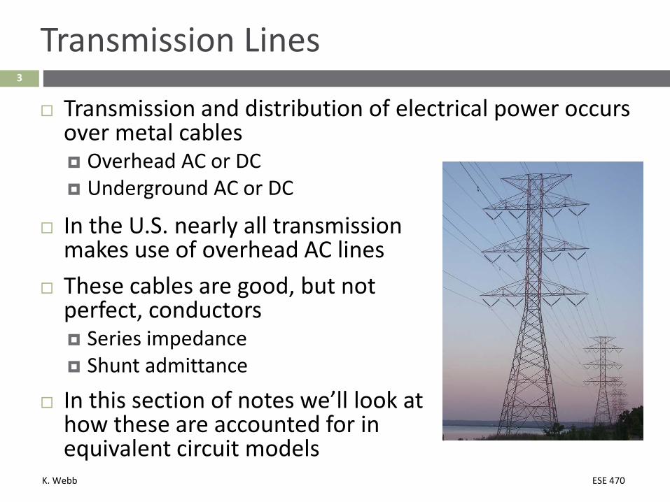
Transmission and distribution of electrical power occurs over metal cables Overhead AC or DC Underground AC or DC
In the U.S. nearly all transmission makes use of overhead AC lines
These cables are good, but not perfect, conductors Series impedance Shunt admittance
In this section of notes we’ll look at how these are accounted for in equivalent circuit models

K. Webb ESE 470
4
Electrical Properties of Transmission Lines
Series resistance Voltage drop (𝐼𝐼𝐼𝐼) and real power loss (𝐼𝐼2𝐼𝐼) along the line Due to finite conductivity of the line
Series inductance Series voltage drop, no real power loss Only self inductance (no mutual inductance) in balanced systems
Shunt conductance Real power loss (𝑉𝑉2𝐺𝐺) Leakage current due to corona effects or leakage at insulators Typically neglected for overhead lines
Shunt capacitance Capacitance to other conductors and to ground Line-charging currents

K. Webb ESE 470
Conductors5

K. Webb ESE 470
6
Conductors
Before getting into transmission line models, we’ll take a look at the conductors themselves
Aluminum is the most common conductor Good conductivity Light weight Low cost Plentiful supply
Most common cable type combines aluminum and steel Aluminum-conductor steel-reinforced (ACSR) Bare, stranded cable Core of steel strands provides strength Outer aluminum strands provide good conductivity

K. Webb ESE 470
7
ACSR Cables
ACSR cables vary based on number of aluminum conductor strands and number of steel reinforcement strands ACSR variants assigned bird code names, e.g.:
Dove: 26/7 Al/Steel stranding Bluebird: 84/19 Al/Steel stranding
Another increasingly popular cable type is all-aluminum-alloy conductor(AAAC) Stronger Lighter Higher conductivity More expensive
source: Glover, Sarma, Overbye

K. Webb ESE 470
8
Cables
Cables are sized to provide the required current-carrying capability or ampacity Number of individual strands Diameter of individual strands
Strand and cable diameter commonly measured in mils1 𝑚𝑚𝑚𝑚𝑚𝑚 = 0.001"
Cross-sectional area often measured in circular mils or cmil Area of a circle with a diameter of 𝑑𝑑 = 1 𝑚𝑚𝑚𝑚𝑚𝑚 = 0.001“
1 𝑐𝑐𝑚𝑚𝑚𝑚𝑚𝑚 = 𝜋𝜋0.001
2
2
= 785 × 10−9 𝑠𝑠𝑠𝑠 𝑚𝑚𝑖𝑖
Area in 𝑐𝑐𝑚𝑚𝑚𝑚𝑚𝑚 of a cable with diameter 𝑑𝑑 𝑚𝑚𝑚𝑚𝑚𝑚:𝐴𝐴 = 𝑑𝑑2

K. Webb ESE 470
9
ACSR Cable
Consider, for example, Falcon ACSR cable 54/19: 54 Al strands with a core of 19 steel strands Al strand diameter: 172 𝑚𝑚𝑚𝑚𝑚𝑚 Al strand area: 172 𝑚𝑚𝑚𝑚𝑚𝑚 2 = 29.584 𝑘𝑘𝑐𝑐𝑚𝑚𝑚𝑚𝑚𝑚
Steel strand diameter: 103 𝑚𝑚𝑚𝑚𝑚𝑚 Steel strand area: 103 𝑚𝑚𝑚𝑚𝑚𝑚 2 = 10.609 𝑘𝑘𝑐𝑐𝑚𝑚𝑚𝑚𝑚𝑚
Cable diameter: 1.545“ Cable area: 1545 𝑚𝑚𝑚𝑚𝑚𝑚 2 = 2387 𝑘𝑘𝑐𝑐𝑚𝑚𝑚𝑚𝑚𝑚
Ampacity: 1380 𝐴𝐴 Weight: 10,777 𝑚𝑚𝑙𝑙/𝑚𝑚𝑚𝑚

K. Webb ESE 470
10
Bundling
Two-, three-, and four-cable bundles are common:
In addition to increasing cable cross-sectional area, ampacity can be increased by adding additional cables to each phase – bundling

K. Webb ESE 470
11
Bundling
Typical bundling: 345 kV: two conductors 500 kV: three conductors 765 kV: four conductors
Advantages of bundling: Lower resistance Lower reactance (inductance) Increased ampacity Reduced electric field gradient surrounding phase conductor Reduced corona Reduced loss, noise, and RF interference
Improved heat dissipation

K. Webb ESE 470
12
Insulators
Cables are supported by towers Must connect, while retaining electrical isolation
Connections are typically made through ceramic or glass insulators
High-voltage lines suspended by strings of insulator discs
One or two strings Two prevents sway
Number of discs dictated by line voltage, e.g.: 4-6 for 69 kV 30-35 for 765 kV

K. Webb ESE 470
13
Transposition
Transmission-line inductance and capacitance determined by geometry Cable size and relative spacing
Consider three phases laid out side-by-side
Phases a and c will have similar inductance and capacitance Inductance and capacitance of phase b will differ

K. Webb ESE 470
14
Transposition
Transposition Switch the position of
each phase twice along the length of the line
Each phase occupies each position for one third of the line length
Line remains balanced

K. Webb ESE 470
Medium- and Short-Line Models15

K. Webb ESE 470
16
Short-Line Model
How we choose to model the electrical characteristics of a transmission line depends on the length of the line
Short-line model: < ~80 𝑘𝑘𝑚𝑚 Lumped model Account only for series impedance Neglect shunt capacitance
𝐼𝐼 and 𝜔𝜔𝜔𝜔 are resistance and reactance per unit length, respectively Each with units of Ω/𝑚𝑚
𝑚𝑚 is the length of the line

K. Webb ESE 470
17
Medium-Line Model
Medium-line model – nominal-𝝅𝝅 model: 80 𝑘𝑘𝑚𝑚 < 𝑚𝑚 < 250 𝑘𝑘𝑚𝑚 Lumped model Now include shunt capacitance
𝑧𝑧 = 𝐼𝐼 + 𝑗𝑗𝜔𝜔𝜔𝜔 Ω/𝑚𝑚 and 𝑍𝑍 = 𝑧𝑧𝑚𝑚 Ω𝑦𝑦 = 𝜔𝜔𝜔𝜔 𝑆𝑆/𝑚𝑚 and 𝑌𝑌 = 𝑦𝑦𝑚𝑚 𝑆𝑆
Still a lumped model All impedances and admittances lumped into one or two circuit
components

K. Webb ESE 470
18
Transmission Lines as Two-Port Networks
Before moving on to a model for longer transmission lines, we’ll look at an alternative tool for characterizing transmission line networks
We can treat transmission lines as general two-port networks
As two-port networks, we can characterize transmission lines with their ABCD parameters or chain parameters

K. Webb ESE 470
19
ABCD Parameters
ABCD (or chain or transmission or cascade) parameters define the following two-port relationships
𝑽𝑽1 = 𝐴𝐴𝑽𝑽2 + 𝐵𝐵𝑰𝑰2𝑰𝑰1 = 𝜔𝜔𝑽𝑽2 + 𝐷𝐷𝑰𝑰2
In matrix form, the chain-parameter equations are𝑽𝑽1𝑰𝑰1
= 𝐴𝐴 𝐵𝐵𝜔𝜔 𝐷𝐷
𝑽𝑽2𝑰𝑰2
𝐴𝐴, 𝐵𝐵, 𝜔𝜔, and 𝐷𝐷 are, in general, complex numbers 𝐴𝐴 and 𝐷𝐷 are dimensionless 𝐵𝐵 is an impedance with units of Ω 𝜔𝜔 is an admittance with units of 𝑆𝑆
𝑉𝑉1 and 𝑉𝑉2 are line-to-neutral voltages
If the network is reciprocal, then 𝐴𝐴𝐷𝐷 − 𝐵𝐵𝜔𝜔 = 1 If the network is symmetric, then 𝐴𝐴 = 𝐷𝐷

K. Webb ESE 470
20
ABCD Parameters – Short-Line Model
Applying KVL around the loop gives our first equation𝑽𝑽𝑆𝑆 − 𝑰𝑰𝑅𝑅𝑍𝑍 − 𝑽𝑽𝑅𝑅 = 0
𝑽𝑽𝑆𝑆 = 𝑽𝑽𝑅𝑅 + 𝑍𝑍𝑰𝑰𝑅𝑅So,
𝐴𝐴 = 1 and 𝐵𝐵 = 𝑍𝑍
We’ll now derive the ABCD parameters for the short-transmission-line model
K. Webb ESE 470
21
ABCD Parameters – Short-Line Model
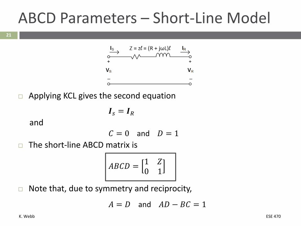
Applying KCL gives the second equation
𝑰𝑰𝑠𝑠 = 𝑰𝑰𝑅𝑅and
𝜔𝜔 = 0 and 𝐷𝐷 = 1 The short-line ABCD matrix is
𝐴𝐴𝐵𝐵𝜔𝜔𝐷𝐷 = 1 𝑍𝑍0 1
Note that, due to symmetry and reciprocity,
𝐴𝐴 = 𝐷𝐷 and 𝐴𝐴𝐷𝐷 − 𝐵𝐵𝜔𝜔 = 1

K. Webb ESE 470
22
ABCD Parameters – Medium-Line Model
Applying KVL around the loop gives our first equation
𝑽𝑽𝑆𝑆 − 𝑰𝑰𝑅𝑅 + 𝑽𝑽𝑅𝑅𝑌𝑌2
𝑍𝑍 − 𝑽𝑽𝑅𝑅 = 0
𝑽𝑽𝑆𝑆 = 1 +𝑌𝑌𝑍𝑍2
𝑽𝑽𝑅𝑅 + 𝑍𝑍𝑰𝑰𝑅𝑅
This is the first chain parameter equation, where
𝐴𝐴 = 1 + 𝑌𝑌𝑌𝑌2
and 𝐵𝐵 = 𝑍𝑍
Next, for the medium-transmission-line model

K. Webb ESE 470
23
ABCD Parameters – Medium-Line Model
For the second equation, apply KCL at the sending end
𝑰𝑰𝑠𝑠 − 𝑽𝑽𝑠𝑠𝑌𝑌2 − 𝑰𝑰𝑅𝑅 − 𝑽𝑽𝑅𝑅
𝑌𝑌2 = 0
Substituting in our previous expression for 𝑉𝑉𝑆𝑆
𝑰𝑰𝑆𝑆 = 𝑽𝑽𝑅𝑅𝑌𝑌2 + 𝑰𝑰𝑅𝑅 + 1 +
𝑌𝑌𝑍𝑍2
𝑌𝑌2 𝑽𝑽𝑅𝑅 +
𝑌𝑌𝑍𝑍2 𝑰𝑰𝑅𝑅
𝑰𝑰𝑆𝑆 = 2 +𝑌𝑌𝑍𝑍2
𝑌𝑌2 𝑽𝑽𝑅𝑅 + 1 +
𝑌𝑌𝑍𝑍2 𝑰𝑰𝑅𝑅
This is the second chain-parameter equation, where
𝜔𝜔 = 1 + 𝑌𝑌𝑌𝑌4
𝑌𝑌 and 𝐷𝐷 = 1 + 𝑌𝑌𝑌𝑌2

K. Webb ESE 470
24
ABCD Parameters – Medium-Line Model
The medium-line chain parameters are
𝐴𝐴𝐵𝐵𝜔𝜔𝐷𝐷 =1 +
𝑌𝑌𝑍𝑍2
𝑍𝑍
1 +𝑌𝑌𝑍𝑍4
𝑌𝑌 1 +𝑌𝑌𝑍𝑍2
Again, note that, due to symmetry and reciprocity, 𝐴𝐴 = 𝐷𝐷 and 𝐴𝐴𝐷𝐷 − 𝐵𝐵𝜔𝜔 = 1
Also note that allowing 𝑌𝑌 → 0 yields the chain parameters for the short-line model

K. Webb ESE 470
25
Cascading Two-Port Networks
ABCD parameters or chain parameters are also called cascade parameters
If we cascade multiple two-port networks, the ABCD parameter matrix for the cascade is the product of the individual ABCD parameter matrices
𝐴𝐴𝐵𝐵𝜔𝜔𝐷𝐷 = 𝐴𝐴1𝐴𝐴2 + 𝐵𝐵1𝜔𝜔2 𝐴𝐴1𝐵𝐵2 + 𝐵𝐵1𝐷𝐷2𝜔𝜔1𝐴𝐴2 + 𝐷𝐷1𝜔𝜔2 𝜔𝜔1𝐵𝐵2 + 𝐷𝐷1𝐷𝐷2

K. Webb ESE 470
26
Cascaded Two-Ports - Example
For example, consider the cascade of the following two two-port networks
ABCD parameters for the first network are
𝐴𝐴𝐵𝐵𝜔𝜔𝐷𝐷1 =1 +
𝑌𝑌1𝑍𝑍12
𝑍𝑍1
1 +𝑌𝑌1𝑍𝑍1
4𝑌𝑌1 1 +
𝑌𝑌1𝑍𝑍12
= 1 + 𝑗𝑗𝑗 2 Ω−4 + 𝑗𝑗𝑗 𝑆𝑆 1 + 𝑗𝑗𝑗
And for the second network
𝐴𝐴𝐵𝐵𝜔𝜔𝐷𝐷2 = 1 𝑍𝑍0 1 = 1 4 Ω
0 1 So the overall ABCD matrix is
𝐴𝐴𝐵𝐵𝜔𝜔𝐷𝐷 =1 + 𝑗𝑗𝑗 6 + 𝑗𝑗𝑗𝑗 Ω
−4 + 𝑗𝑗𝑗 𝑆𝑆 −15 + 𝑗𝑗𝑗𝑗

K. Webb ESE 470
27
Cascaded Two-Ports - Example
If a sending-end voltage of 𝑽𝑽𝑆𝑆 = 𝑗𝑗0∠0° 𝑉𝑉 is applied, and no load is connected, what is the receiving-end voltage?
𝑽𝑽𝑆𝑆 = 𝑗𝑗0∠0° 𝑉𝑉 and 𝑰𝑰𝑅𝑅 = 0 𝐴𝐴
𝑽𝑽𝑆𝑆 = 𝐴𝐴𝑽𝑽𝑅𝑅 + 𝐵𝐵𝑰𝑰𝑅𝑅1𝑗0∠0° = 1 + 𝑗𝑗𝑗 𝑉𝑉𝑅𝑅
The no-load receiving-end voltage is
𝑽𝑽𝑅𝑅 =𝑗𝑗0∠0°1 + 𝑗𝑗𝑗
= 7.06 − 𝑗𝑗𝑗𝑗.2 𝑉𝑉
𝑽𝑽𝑅𝑅 = 29.𝑗∠ − 75.9𝑗° 𝑉𝑉
K. Webb ESE 470
28
Voltage Regulation
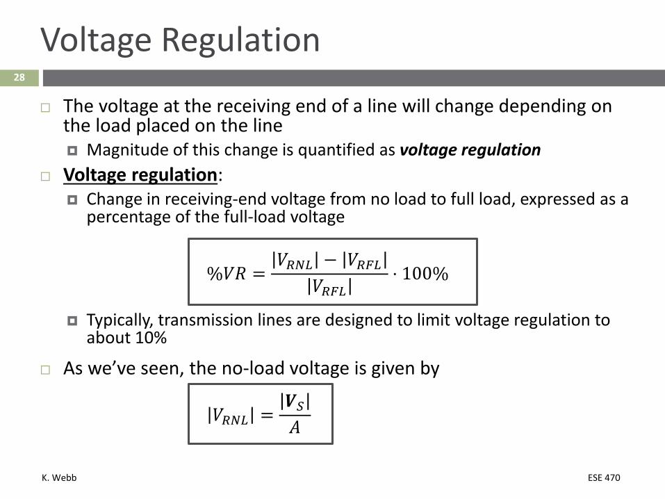
The voltage at the receiving end of a line will change depending on the load placed on the line Magnitude of this change is quantified as voltage regulation
Voltage regulation: Change in receiving-end voltage from no load to full load, expressed as a
percentage of the full-load voltage
%𝑉𝑉𝐼𝐼 =𝑉𝑉𝑅𝑅𝑅𝑅𝑅𝑅 − 𝑉𝑉𝑅𝑅𝑅𝑅𝑅𝑅
𝑉𝑉𝑅𝑅𝑅𝑅𝑅𝑅⋅ 100%
Typically, transmission lines are designed to limit voltage regulation to about 10%
As we’ve seen, the no-load voltage is given by
𝑉𝑉𝑅𝑅𝑅𝑅𝑅𝑅 =𝑽𝑽𝑆𝑆𝐴𝐴
K. Webb ESE 470
29
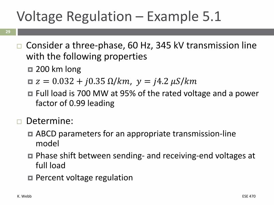
Voltage Regulation – Example 5.1
Consider a three-phase, 60 Hz, 345 kV transmission line with the following properties 200 km long 𝑧𝑧 = 0.032 + 𝑗𝑗0.35 Ω/𝑘𝑘𝑚𝑚, 𝑦𝑦 = 𝑗𝑗𝑗.2 𝜇𝜇𝑆𝑆/𝑘𝑘𝑚𝑚 Full load is 700 MW at 95% of the rated voltage and a power
factor of 0.99 leading
Determine: ABCD parameters for an appropriate transmission-line
model Phase shift between sending- and receiving-end voltages at
full load Percent voltage regulation
K. Webb ESE 470
30
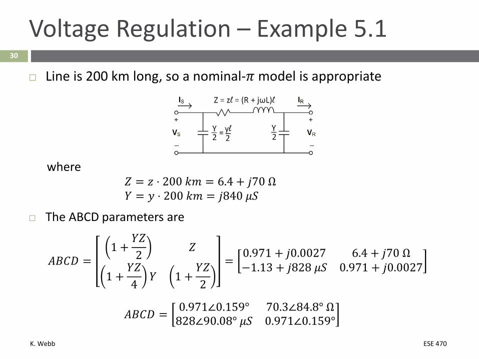
Voltage Regulation – Example 5.1
Line is 200 km long, so a nominal-𝜋𝜋 model is appropriate
where𝑍𝑍 = 𝑧𝑧 ⋅ 200 𝑘𝑘𝑚𝑚 = 6.4 + 𝑗𝑗𝑗0 Ω𝑌𝑌 = 𝑦𝑦 ⋅ 200 𝑘𝑘𝑚𝑚 = 𝑗𝑗𝑗𝑗0 𝜇𝜇𝑆𝑆
The ABCD parameters are
𝐴𝐴𝐵𝐵𝜔𝜔𝐷𝐷 =1 +
𝑌𝑌𝑍𝑍2 𝑍𝑍
1 +𝑌𝑌𝑍𝑍4 𝑌𝑌 1 +
𝑌𝑌𝑍𝑍2
= 0.971 + 𝑗𝑗0.0027 6.4 + 𝑗𝑗𝑗0 Ω−1.13 + 𝑗𝑗𝑗𝑗𝑗 𝜇𝜇𝑆𝑆 0.971 + 𝑗𝑗0.0027
𝐴𝐴𝐵𝐵𝜔𝜔𝐷𝐷 = 0.9𝑗𝑗∠0.𝑗59° 70.3∠𝑗𝑗.𝑗° Ω𝑗𝑗𝑗∠90.0𝑗° 𝜇𝜇𝑆𝑆 0.9𝑗𝑗∠0.𝑗59°

K. Webb ESE 470
31
Voltage Regulation – Example 5.1
At full load the line-to-line receiving-end voltage is 𝑉𝑉𝑅𝑅𝑅𝑅𝑅𝑅 = 345 𝑘𝑘𝑉𝑉 ⋅ 0.95 = 327.8 𝑘𝑘𝑉𝑉𝑅𝑅𝑅𝑅
And the line-to-neutral voltage is
𝑉𝑉𝑅𝑅𝑅𝑅𝑅𝑅 =327.8 𝑘𝑘𝑉𝑉𝑅𝑅𝑅𝑅
3= 189.2 𝑘𝑘𝑉𝑉𝑅𝑅𝑅𝑅
Using the receiving-end voltage as the reference, the receiving-end voltage phasor is
𝑽𝑽𝑅𝑅 = 189.𝑗∠0° 𝑘𝑘𝑉𝑉
We know that the load power is given by𝑃𝑃 = 3𝑉𝑉𝑅𝑅𝑅𝑅𝑅𝑅𝐼𝐼𝑅𝑅 cos 𝜃𝜃
𝜃𝜃 is the power-factor angle (leading, so it’s negative)𝜃𝜃 = − cos−1 𝑝𝑝. 𝑓𝑓. = − cos−1 0.99 = −8.𝑗°

K. Webb ESE 470
32
Voltage Regulation – Example 5.1
The receiving-end current phasor is
𝑰𝑰𝑅𝑅 =𝑃𝑃
3𝑉𝑉𝑅𝑅𝑅𝑅𝑅𝑅 cos 𝜃𝜃∠ − 𝜃𝜃 =
700 𝑀𝑀𝑀𝑀3 ⋅ 189.2 𝑘𝑘𝑉𝑉 ⋅ 0.99
∠𝑗.𝑗°
𝑰𝑰𝑅𝑅 = 1.𝑗5∠𝑗.𝑗° 𝑘𝑘𝐴𝐴
To determine the phase shift from sending to receiving end, use chain parameters to determine 𝑽𝑽𝑆𝑆 (line-to-neutral)
𝑽𝑽𝑆𝑆 = 𝐴𝐴𝑽𝑽𝑅𝑅 + 𝐵𝐵𝑰𝑰𝑅𝑅𝑽𝑽𝑆𝑆 = 0.9𝑗𝑗∠0.𝑗59° ⋅ 189.𝑗∠0° 𝑘𝑘𝑉𝑉
+70.3∠𝑗𝑗.𝑗° Ω ⋅ 1.𝑗5∠𝑗.𝑗° 𝑘𝑘𝐴𝐴
𝑽𝑽𝑆𝑆 = 199.𝑗∠𝑗𝑗.𝑗° 𝑘𝑘𝑉𝑉LN
So, the phase shift along the line is −26.𝑗°

K. Webb ESE 470
33
Voltage Regulation – Example 5.1
The percent voltage regulation is given by
%𝑉𝑉𝐼𝐼 =𝑉𝑉𝑅𝑅𝑅𝑅𝑅𝑅 − 𝑉𝑉𝑅𝑅𝑅𝑅𝑅𝑅
𝑉𝑉𝑅𝑅𝑅𝑅𝑅𝑅⋅ 100%
The line-to-neutral no-load voltage is
𝑉𝑉𝑅𝑅𝑅𝑅𝑅𝑅 =𝑽𝑽𝑆𝑆𝐴𝐴
=199.𝑗∠𝑗𝑗.𝑗°
0.9𝑗𝑗∠0.𝑗59°= 205.8 𝑘𝑘𝑉𝑉
The full-load line-to-neutral voltage was given to be𝑉𝑉𝑅𝑅𝑅𝑅𝑅𝑅 = 189.2 𝑘𝑘𝑉𝑉
So, the percent voltage regulation is
%𝑉𝑉𝐼𝐼 =205.8 𝑘𝑘𝑉𝑉 − 189.2 𝑘𝑘𝑉𝑉
189.2 𝑘𝑘𝑉𝑉⋅ 100% = 8.7%
K. Webb ESE 470
Exact Transmission-Line Equations34

K. Webb ESE 470
35
Distributed Transmission Line Model
The medium- and short-line models are lumped models All series impedance lumped into one element Shunt admittances lumped into two elements
Real lines are distributed networks Lumped models are inaccurate for long lines
To treat a line as a distributed network, consider the impedance and admittance of a segment of differential length, Δ𝑥𝑥

K. Webb ESE 470
36
Transmission Line Differential Equations
Apply KVL around the differential length of line
𝑽𝑽 𝑥𝑥 + Δ𝑥𝑥 = 𝑽𝑽 𝑥𝑥 + 𝑰𝑰 𝑥𝑥 𝑧𝑧Δ𝑥𝑥𝑽𝑽 𝑥𝑥+Δ𝑥𝑥 −𝑽𝑽 𝑥𝑥
Δ𝑥𝑥= 𝑧𝑧𝑰𝑰 𝑥𝑥 (1)
If we let the length of the line segment, Δ𝑥𝑥, go to zero, we get𝑑𝑑𝑽𝑽 𝑥𝑥𝑑𝑑𝑥𝑥
= 𝑧𝑧𝑰𝑰 𝑥𝑥 (2)
A first-order differential equation This is a second-order segment, so we need a second first-order
differential equation to describe it completely Apply KCL at 𝑥𝑥 + Δ𝑥𝑥
𝑰𝑰 𝑥𝑥 + Δ𝑥𝑥 = 𝑰𝑰 𝑥𝑥 + 𝑽𝑽 𝑥𝑥 + Δ𝑥𝑥 𝑦𝑦Δ𝑥𝑥𝑰𝑰 𝑥𝑥+Δ𝑥𝑥 −𝑰𝑰 𝑥𝑥
Δ𝑥𝑥= 𝑦𝑦𝑽𝑽 𝑥𝑥 + Δ𝑥𝑥 (3)

K. Webb ESE 470
37
Transmission Line Differential Equations
Again, letting Δ𝑥𝑥 → 0𝑑𝑑𝑰𝑰 𝑥𝑥𝑑𝑑𝑥𝑥
= 𝑦𝑦𝑽𝑽 𝑥𝑥 (4)
Our goal is a single differential equation in 𝑽𝑽 𝑥𝑥 to describe the segment of transmission line Must eliminate 𝑰𝑰 𝑥𝑥
Solving (2) for 𝑰𝑰 𝑥𝑥 and differentiating gives𝑑𝑑𝑰𝑰 𝑥𝑥𝑑𝑑𝑥𝑥
= 1𝑌𝑌𝑑𝑑2𝑽𝑽 𝑥𝑥𝑑𝑑𝑥𝑥2
(5)
Substituting (5) into (4) yields the single second-order differential equation for the line segment
𝑑𝑑2𝑽𝑽 𝑥𝑥𝑑𝑑𝑥𝑥2
− 𝑧𝑧𝑦𝑦𝑽𝑽 𝑥𝑥 = 0 (6)
K. Webb ESE 470
38
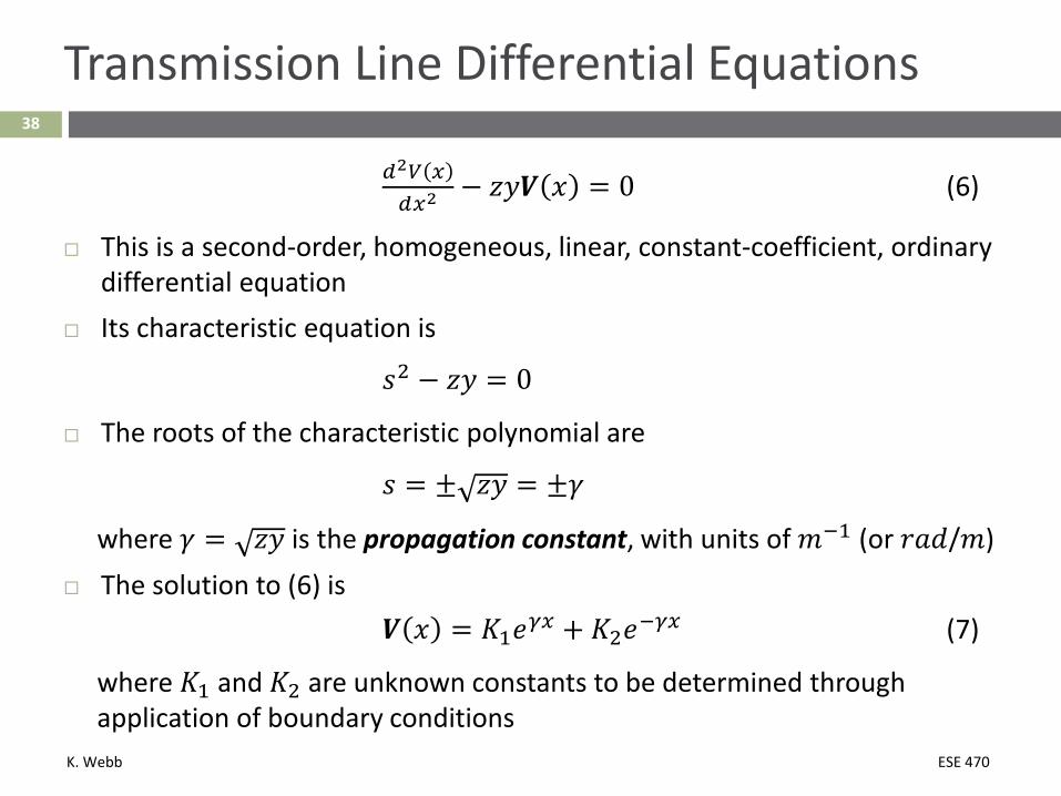
Transmission Line Differential Equations
𝑑𝑑2𝑉𝑉 𝑥𝑥𝑑𝑑𝑥𝑥2
− 𝑧𝑧𝑦𝑦𝑽𝑽 𝑥𝑥 = 0 (6)
This is a second-order, homogeneous, linear, constant-coefficient, ordinary differential equation
Its characteristic equation is
𝑠𝑠2 − 𝑧𝑧𝑦𝑦 = 0
The roots of the characteristic polynomial are
𝑠𝑠 = ± 𝑧𝑧𝑦𝑦 = ±𝛾𝛾
where 𝛾𝛾 = 𝑧𝑧𝑦𝑦 is the propagation constant, with units of 𝑚𝑚−1 (or 𝑟𝑟𝑟𝑟𝑑𝑑/𝑚𝑚) The solution to (6) is
𝑽𝑽 𝑥𝑥 = 𝐾𝐾1𝑒𝑒𝛾𝛾𝑥𝑥 + 𝐾𝐾2𝑒𝑒−𝛾𝛾𝑥𝑥 (7)
where 𝐾𝐾1 and 𝐾𝐾2 are unknown constants to be determined through application of boundary conditions

K. Webb ESE 470
39
Transmission Line Differential Equations
We can get an expression for current by differentiating (7) and substituting back into (2)
𝑑𝑑𝑉𝑉 𝑥𝑥𝑑𝑑𝑥𝑥
= 𝛾𝛾𝐾𝐾1𝑒𝑒𝛾𝛾𝑥𝑥 − 𝛾𝛾𝐾𝐾2𝑒𝑒−𝛾𝛾𝑥𝑥 = 𝑧𝑧𝑰𝑰 𝑥𝑥
Solving for 𝑰𝑰 𝑥𝑥
𝑰𝑰 𝑥𝑥 = 𝐾𝐾1𝑒𝑒𝛾𝛾𝛾𝛾−𝐾𝐾2𝑒𝑒−𝛾𝛾𝛾𝛾
⁄𝑧𝑧 𝛾𝛾(8)
The term in the denominator of (8) is the characteristic impedance of the line, 𝑍𝑍𝑐𝑐, with units of ohms (Ω)
𝑍𝑍𝑐𝑐 = 𝑧𝑧𝛾𝛾
= 𝑧𝑧𝑧𝑧𝑧𝑧
= 𝑧𝑧𝑧𝑧
(9)

K. Webb ESE 470
40
Transmission Line Differential Equations
Using (9), (8) becomes
𝑰𝑰 𝑥𝑥 = 𝐾𝐾1𝑒𝑒𝛾𝛾𝛾𝛾−𝐾𝐾2𝑒𝑒−𝛾𝛾𝛾𝛾
𝑌𝑌𝑐𝑐(10)
We can now apply boundary conditions to determine the two unknown coefficients, 𝐾𝐾1 and 𝐾𝐾2
At the receiving end of the line, which we’ll define to be 𝑥𝑥 = 0, we have
𝑽𝑽 0 = 𝑽𝑽𝑅𝑅 and 𝑰𝑰 0 = 𝑰𝑰𝑅𝑅So,
𝑽𝑽 0 = 𝐾𝐾1 + 𝐾𝐾2 = 𝑽𝑽𝑅𝑅
𝑰𝑰 0 =𝐾𝐾1 − 𝐾𝐾2𝑍𝑍𝑐𝑐
= 𝑰𝑰𝑅𝑅

K. Webb ESE 470
41
Transmission Line Differential Equations
Solving each equation for 𝐾𝐾2𝐾𝐾2 = 𝑽𝑽𝑅𝑅 − 𝐾𝐾1 = 𝐾𝐾1 − 𝑍𝑍𝑐𝑐𝑰𝑰𝑅𝑅
Solving for 𝐾𝐾1, then back-substituting to solve for 𝐾𝐾2gives
𝐾𝐾1 = 𝑽𝑽𝑅𝑅+𝑌𝑌𝑐𝑐𝑰𝑰𝑅𝑅2
𝐾𝐾2 = 𝑽𝑽𝑅𝑅−𝑌𝑌𝑐𝑐𝑰𝑰𝑅𝑅2
Substituting into (7) and (10)
𝑽𝑽 𝑥𝑥 = 𝑽𝑽𝑅𝑅+𝑌𝑌𝑐𝑐𝑰𝑰𝑅𝑅2
𝑒𝑒𝛾𝛾𝑥𝑥 + 𝑽𝑽𝑅𝑅−𝑌𝑌𝑐𝑐𝑰𝑰𝑅𝑅2
𝑒𝑒−𝛾𝛾𝑥𝑥 (11)
𝑰𝑰 𝑥𝑥 = 𝑽𝑽𝑅𝑅+𝑌𝑌𝑐𝑐𝑰𝑰𝑅𝑅2𝑌𝑌𝑐𝑐
𝑒𝑒𝛾𝛾𝑥𝑥 − 𝑽𝑽𝑅𝑅−𝑌𝑌𝑐𝑐𝑰𝑰𝑅𝑅2𝑌𝑌𝑐𝑐
𝑒𝑒−𝛾𝛾𝑥𝑥 (12)

K. Webb ESE 470
42
Transmission Line Differential Equations
Collecting 𝑉𝑉𝑅𝑅 and 𝐼𝐼𝑅𝑅 terms in (11) and (12)
𝑽𝑽 𝑥𝑥 = 𝑒𝑒𝛾𝛾𝛾𝛾+𝑒𝑒−𝛾𝛾𝛾𝛾
2𝑽𝑽𝑅𝑅 + 𝑍𝑍𝑐𝑐
𝑒𝑒𝛾𝛾𝛾𝛾−𝑒𝑒−𝛾𝛾𝛾𝛾
2𝑰𝑰𝑅𝑅 (13)
𝑰𝑰 𝑥𝑥 = 1𝑌𝑌𝑐𝑐
𝑒𝑒𝛾𝛾𝛾𝛾−𝑒𝑒−𝛾𝛾𝛾𝛾
2𝑽𝑽𝑅𝑅 + 𝑒𝑒𝛾𝛾𝛾𝛾+𝑒𝑒−𝛾𝛾𝛾𝛾
2𝑰𝑰𝑅𝑅 (14)
The terms in parentheses can be represented as hyperbolic functions
𝑽𝑽 𝑥𝑥 = cosh 𝛾𝛾𝑥𝑥 𝑽𝑽𝑅𝑅 + 𝑍𝑍𝑐𝑐 sinh 𝛾𝛾𝑥𝑥 𝑰𝑰𝑅𝑅 (15)
𝑰𝑰 𝑥𝑥 = 1𝑌𝑌𝑐𝑐
sinh 𝛾𝛾𝑥𝑥 𝑽𝑽𝑅𝑅 + cosh 𝛾𝛾𝑥𝑥 𝑰𝑰𝑅𝑅 (16)

K. Webb ESE 470
43
Transmission Line Differential Equations
Equations (15) and (16) give the chain parameters for the two-port network between a point at location 𝑥𝑥 along the line and the receiving end
𝐴𝐴𝐵𝐵𝜔𝜔𝐷𝐷 𝑥𝑥 =cosh 𝛾𝛾𝑥𝑥 𝑍𝑍𝑐𝑐 sinh 𝛾𝛾𝑥𝑥
1𝑍𝑍𝑐𝑐
sinh 𝛾𝛾𝑥𝑥 cosh 𝛾𝛾𝑥𝑥
For chain parameters between sending and receiving ends, we set 𝑥𝑥 = 𝑚𝑚
𝐴𝐴𝐵𝐵𝜔𝜔𝐷𝐷 =cosh 𝛾𝛾𝑚𝑚 𝑍𝑍𝑐𝑐 sinh 𝛾𝛾𝑚𝑚
1𝑍𝑍𝑐𝑐
sinh 𝛾𝛾𝑚𝑚 cosh 𝛾𝛾𝑚𝑚

K. Webb ESE 470
44
Propagation Constant
We defined the propagation constant as𝛾𝛾 = 𝑧𝑧𝑦𝑦
This is, in general, a complex value𝛾𝛾 = 𝛼𝛼 + 𝑗𝑗𝑗𝑗 (17)
The real part, 𝛼𝛼, is the attenuation constant Represents loss along the line Due to series resistance and/or shunt conductance
The imaginary part, 𝑗𝑗, is the phase constant Represents change in phase along the line Due to series reactance and/or shunt susceptance

K. Webb ESE 470
45
Long-Line Equivalent 𝜋𝜋 Circuit
Now that we have exact ABCD parameters for a distributed transmission line, we can create an equivalent 𝜋𝜋 circuit
Here we’re using 𝑍𝑍𝑍 and 𝑌𝑌𝑍 to distinguish from 𝑍𝑍 = 𝑧𝑧𝑚𝑚 and 𝑌𝑌 = 𝑦𝑦𝑚𝑚 of the lumped, nominal 𝜋𝜋-circuit model
Equating the ABCD parameters with those for the equivalent 𝜋𝜋circuit above
cosh 𝛾𝛾𝑚𝑚 𝑍𝑍𝑐𝑐 sinh 𝛾𝛾𝑚𝑚1𝑍𝑍𝑐𝑐
sinh 𝛾𝛾𝑚𝑚 cosh 𝛾𝛾𝑚𝑚 =1 +
𝑌𝑌′𝑍𝑍′
2𝑍𝑍𝑍
𝑌𝑌′ 1 +𝑌𝑌′𝑍𝑍′
41 +
𝑌𝑌′𝑍𝑍′
2

K. Webb ESE 470
46
Long-Line Equivalent 𝜋𝜋 Circuit
Equating the 𝐵𝐵 parameters, we see that𝑍𝑍′ = 𝑍𝑍𝑐𝑐 sinh 𝛾𝛾𝑚𝑚 (18)
Using (18) in the 𝐴𝐴-parameter equation gives
1 +𝑌𝑌′
2𝑍𝑍𝑐𝑐 sinh 𝛾𝛾𝑚𝑚 = cosh 𝛾𝛾𝑚𝑚
𝑌𝑌′
2 =cosh 𝛾𝛾𝑚𝑚 − 1𝑍𝑍𝑐𝑐 sinh 𝛾𝛾𝑚𝑚 =
tanh 𝛾𝛾𝑚𝑚2
𝑍𝑍𝑐𝑐
The equivalent 𝜋𝜋 circuit for long transmission lines (>250 km) is

K. Webb ESE 470
47
Long-Line vs. Medium-Line Models
We can compare this equivalent 𝜋𝜋 circuit with the nominal 𝜋𝜋 circuit used for medium-length lines, where
𝑍𝑍 = 𝑧𝑧𝑚𝑚 and 𝑌𝑌2
= 𝑦𝑦 𝑙𝑙2
Rewriting (18) using the definition for characteristic impedance,
𝑍𝑍′ = 𝑧𝑧𝑧𝑧
sinh 𝛾𝛾𝑚𝑚 = 𝑧𝑧𝑚𝑚 𝑧𝑧𝑧𝑧sinh 𝛾𝛾𝑙𝑙
𝑧𝑧𝑙𝑙
𝑍𝑍′ = 𝑧𝑧𝑚𝑚 sinh 𝛾𝛾𝑙𝑙𝑧𝑧𝑧𝑧 𝑙𝑙
𝑍𝑍′ = 𝑍𝑍 sinh 𝛾𝛾𝑙𝑙𝛾𝛾𝑙𝑙
(20)
We see that the series impedance of the long-line model is equal to that of the medium-line model, multiplied by a correction factor

K. Webb ESE 470
48
Long-Line vs. Medium-Line Models
Doing the same for the shunt admittance, we have
𝑌𝑌′
2= 𝑧𝑧
𝑧𝑧tanh �𝛾𝛾𝑙𝑙 2 = 𝑧𝑧𝑙𝑙
2𝑧𝑧𝑧𝑧
tanh �𝛾𝛾𝛾𝛾 2�𝑦𝑦𝛾𝛾2
𝑌𝑌′
2= 𝑧𝑧𝑙𝑙
2
tanh �𝛾𝛾𝛾𝛾 2
𝑧𝑧𝑧𝑧𝛾𝛾2
𝑌𝑌′
2= 𝑌𝑌
2
tanh �𝛾𝛾𝛾𝛾 2�𝛾𝛾𝛾𝛾 2
Again, we see a similar correction factor relating the admittance, 𝑌𝑌, of the lumped, nominal 𝜋𝜋 circuit to the admittance of the distributed, equivalent 𝜋𝜋 circuit, 𝑌𝑌𝑍

K. Webb ESE 470
Lossless Lines49

K. Webb ESE 470
50
Lossless Lines
Transmission line models can be simplified significantly if we neglect loss Sacrifice accuracy for the sake of simplicity
Series resistance, 𝐼𝐼, and shunt conductance, 𝐺𝐺, are the model parameters accounting for loss Let 𝐼𝐼 → 0 and 𝐺𝐺 → 0 – (we’ve already assumed 𝐺𝐺 = 0)
Propagation constant for a lossless line is 𝛾𝛾 = 𝑗𝑗𝑗𝑗
The attenuation constant is now zero, 𝛼𝛼 → 0
𝛾𝛾 = 𝑧𝑧𝑦𝑦 = 𝑗𝑗𝜔𝜔𝜔𝜔 ⋅ 𝑗𝑗𝜔𝜔𝜔𝜔 = 𝑗𝑗𝜔𝜔 𝜔𝜔𝜔𝜔 = 𝑗𝑗𝑗𝑗
𝑗𝑗 = 𝜔𝜔 𝜔𝜔𝜔𝜔

K. Webb ESE 470
51
Lossless Lines – ABCD Parameters
Using the propagation constant for a lossless line, the distributed model chain parameters become
𝐴𝐴 𝑥𝑥 = 𝐷𝐷 𝑥𝑥 = cosh 𝑗𝑗𝑗𝑗𝑥𝑥 =𝑒𝑒𝑗𝑗𝑗𝑗𝑥𝑥 + 𝑒𝑒−𝑗𝑗𝑗𝑗𝑥𝑥
2𝐴𝐴 𝑥𝑥 = 𝐷𝐷 𝑥𝑥 = cos 𝑗𝑗𝑥𝑥
𝐵𝐵 𝑥𝑥 = 𝑍𝑍𝑐𝑐 sinh 𝑗𝑗𝑗𝑗𝑥𝑥 = 𝑍𝑍𝑐𝑐𝑒𝑒𝑗𝑗𝑗𝑗𝑥𝑥 − 𝑒𝑒−𝑗𝑗𝑗𝑗𝑥𝑥
2𝐵𝐵 𝑥𝑥 = 𝑗𝑗𝑍𝑍𝑐𝑐 sin 𝑗𝑗𝑥𝑥
𝜔𝜔 𝑥𝑥 =1𝑍𝑍𝑐𝑐
sinh 𝑗𝑗𝑗𝑗𝑥𝑥 =1𝑍𝑍𝑐𝑐𝑒𝑒𝑗𝑗𝑗𝑗𝑥𝑥 − 𝑒𝑒−𝑗𝑗𝑗𝑗𝑥𝑥
2
𝜔𝜔 𝑥𝑥 = 𝑗𝑗sin 𝑗𝑗𝑥𝑥𝑍𝑍𝑐𝑐

K. Webb ESE 470
52
Lossless Lines – ABCD Parameters
Chain parameters at a distance 𝑥𝑥 from the end of a lossless line are
𝐴𝐴𝐵𝐵𝜔𝜔𝐷𝐷 𝑥𝑥 =cos 𝑗𝑗𝑥𝑥 𝑗𝑗𝑍𝑍𝑐𝑐 sin 𝑗𝑗𝑥𝑥
𝑗𝑗sin 𝑗𝑗𝑥𝑥𝑍𝑍𝑐𝑐
cos 𝑗𝑗𝑥𝑥
And at the sending end of a line of length 𝑚𝑚, 𝑥𝑥 → 𝑚𝑚, and we have
𝐴𝐴𝐵𝐵𝜔𝜔𝐷𝐷 =cos 𝑗𝑗𝑚𝑚 𝑗𝑗𝑍𝑍𝑐𝑐 sin 𝑗𝑗𝑚𝑚
𝑗𝑗sin 𝑗𝑗𝑚𝑚𝑍𝑍𝑐𝑐
cos 𝑗𝑗𝑚𝑚
The characteristic impedance of the lossless line is called the surgeimpedance
𝑍𝑍𝑐𝑐 =𝑧𝑧𝑦𝑦 =
𝑗𝑗𝜔𝜔𝜔𝜔𝑗𝑗𝜔𝜔𝜔𝜔 =
𝜔𝜔𝜔𝜔

K. Webb ESE 470
53
Equivalent 𝜋𝜋 Circuit – Lossless Line
For the lossless line𝛾𝛾 = 𝑗𝑗𝑗𝑗
so,
𝑍𝑍′ = 𝑍𝑍𝑐𝑐 sinh 𝑗𝑗𝑗𝑗𝑚𝑚 = 𝑗𝑗𝜔𝜔𝜔𝜔 sin 𝑗𝑗𝑚𝑚 = 𝑗𝑗𝑋𝑋′
and,
𝑌𝑌′
2 =tanh 𝑗𝑗𝑗𝑗𝑚𝑚
2𝑍𝑍𝑐𝑐
= 𝑗𝑗tan 𝑗𝑗𝑚𝑚
2𝑍𝑍𝑐𝑐
K. Webb ESE 470
54
Wavelength
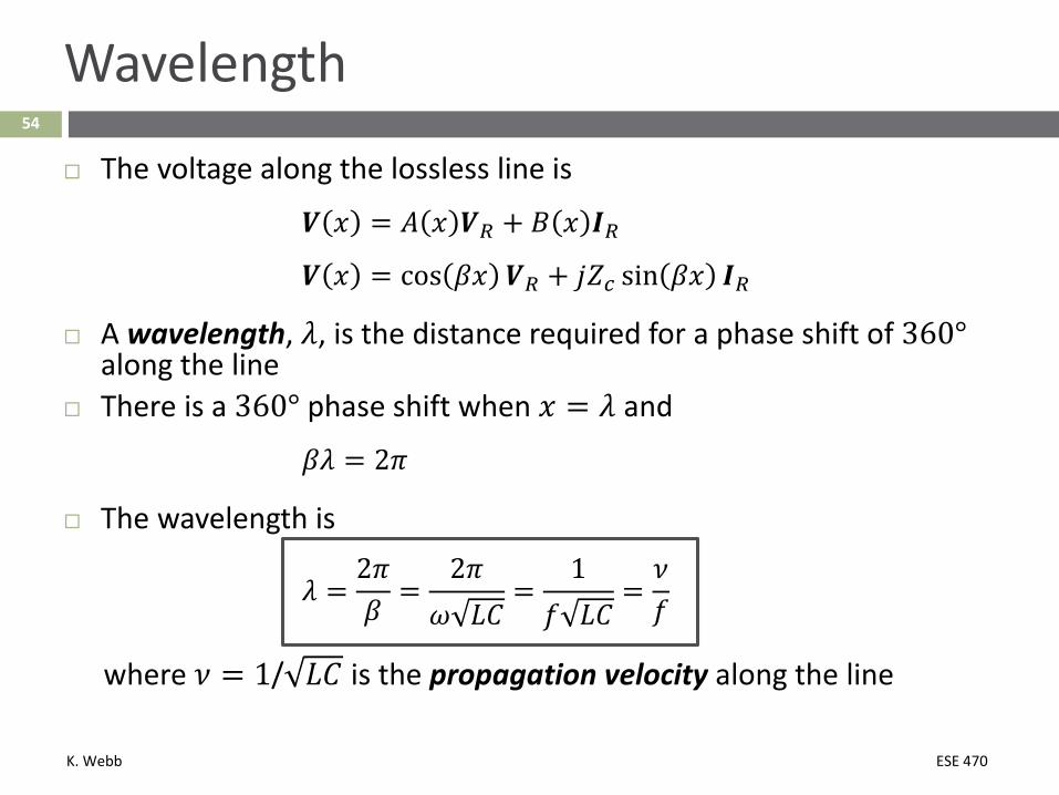
The voltage along the lossless line is
𝑽𝑽 𝑥𝑥 = 𝐴𝐴 𝑥𝑥 𝑽𝑽𝑅𝑅 + 𝐵𝐵 𝑥𝑥 𝑰𝑰𝑅𝑅𝑽𝑽 𝑥𝑥 = cos 𝑗𝑗𝑥𝑥 𝑽𝑽𝑅𝑅 + 𝑗𝑗𝑍𝑍𝑐𝑐 sin 𝑗𝑗𝑥𝑥 𝑰𝑰𝑅𝑅
A wavelength, 𝜆𝜆, is the distance required for a phase shift of 3𝑗0°along the line
There is a 3𝑗0° phase shift when 𝑥𝑥 = 𝜆𝜆 and
𝑗𝑗𝜆𝜆 = 𝑗𝜋𝜋
The wavelength is
𝜆𝜆 =𝑗𝜋𝜋𝑗𝑗
=𝑗𝜋𝜋
𝜔𝜔 𝜔𝜔𝜔𝜔=
1𝑓𝑓 𝜔𝜔𝜔𝜔
=𝜈𝜈𝑓𝑓
where 𝜈𝜈 = 1/ 𝜔𝜔𝜔𝜔 is the propagation velocity along the line

K. Webb ESE 470
55
Wavelength
For overhead transmission lines, 𝜈𝜈 ≈ 𝑐𝑐 ≈ 3 × 10⁸𝑚𝑚/𝑠𝑠
That is, electrical waves propagate along the line at roughly the speed of light
At 60 Hz, the wavelength is
𝜆𝜆 =𝜈𝜈𝑓𝑓
=3 × 10⁸
60 = 5000 𝑘𝑘𝑚𝑚
This is approximately the distance across the U.S. Most transmission lines are significantly shorter than a
wavelength

K. Webb ESE 470
56
Surge Impedance Loading (SIL)
Surge impedance loading (SIL) The power delivered by a transmission line to a resistive load whose impedance
is equal to the surge impedance, 𝑍𝑍𝑐𝑐, of that transmission line At SIL, the load current is
𝑰𝑰𝑅𝑅 =𝑽𝑽𝑅𝑅𝑍𝑍𝑐𝑐
The voltage along the line is
𝑽𝑽 𝑥𝑥 = cos 𝑗𝑗𝑥𝑥 𝑽𝑽𝑅𝑅 + 𝑗𝑗𝑍𝑍𝑐𝑐 sin 𝑗𝑗𝑥𝑥 𝑰𝑰𝑅𝑅
𝑽𝑽 𝑥𝑥 = cos 𝑗𝑗𝑥𝑥 𝑽𝑽𝑅𝑅 + 𝑗𝑗𝑍𝑍𝑐𝑐 sin 𝑗𝑗𝑥𝑥𝑽𝑽𝑅𝑅𝑍𝑍𝑐𝑐
𝑽𝑽 𝑥𝑥 = 𝑽𝑽𝑅𝑅 cos 𝑗𝑗𝑥𝑥 + 𝑗𝑗 sin 𝑗𝑗𝑥𝑥
𝑽𝑽 𝑥𝑥 = 𝑽𝑽𝑅𝑅∠𝑗𝑗𝑥𝑥
Note that at SIL, the magnitude of the voltage is constant along the line A flat voltage profile

K. Webb ESE 470
57
Surge Impedance Loading (SIL)
At SIL, the current along the line is given by
𝑰𝑰 𝑥𝑥 = 𝑗𝑗sin 𝑗𝑗𝑥𝑥𝑍𝑍𝑐𝑐
𝑽𝑽𝑅𝑅 + cos 𝑗𝑗𝑥𝑥𝑽𝑽𝑅𝑅𝑍𝑍𝑐𝑐
𝑰𝑰 𝑥𝑥 =𝑽𝑽𝑅𝑅𝑍𝑍𝑐𝑐
cos 𝑗𝑗𝑥𝑥 + 𝑗𝑗 sin 𝑗𝑗𝑥𝑥
𝑰𝑰 𝑥𝑥 =𝑽𝑽𝑅𝑅𝑍𝑍𝑐𝑐
∠𝑗𝑗𝑥𝑥
The complex power along the line is
𝑺𝑺 𝑥𝑥 = 𝑽𝑽 𝑥𝑥 𝑰𝑰 𝑥𝑥 ∗ = 𝑽𝑽𝑅𝑅∠𝑗𝑗𝑥𝑥𝑽𝑽𝑅𝑅𝑍𝑍𝑐𝑐
∠𝑗𝑗𝑥𝑥∗
𝑺𝑺 𝑥𝑥 =𝑽𝑽𝑅𝑅 2
𝑍𝑍𝑐𝑐= 𝑃𝑃 𝑥𝑥 + 𝑗𝑗𝑗𝑗 𝑥𝑥
At SIL Power flow is independent of position along the line Reactive power is zero
K. Webb ESE 470
58
Surge Impedance Loading (SIL)
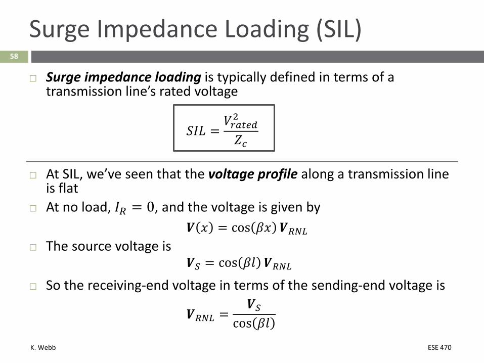
Surge impedance loading is typically defined in terms of a transmission line’s rated voltage
𝑆𝑆𝐼𝐼𝜔𝜔 =𝑉𝑉𝑟𝑟𝑟𝑟𝑟𝑟𝑒𝑒𝑑𝑑2
𝑍𝑍𝑐𝑐
At SIL, we’ve seen that the voltage profile along a transmission line is flat
At no load, 𝐼𝐼𝑅𝑅 = 0, and the voltage is given by𝑽𝑽 𝑥𝑥 = cos 𝑗𝑗𝑥𝑥 𝑽𝑽𝑅𝑅𝑅𝑅𝑅𝑅
The source voltage is𝑽𝑽𝑆𝑆 = cos 𝑗𝑗𝑚𝑚 𝑽𝑽𝑅𝑅𝑅𝑅𝑅𝑅
So the receiving-end voltage in terms of the sending-end voltage is
𝑽𝑽𝑅𝑅𝑅𝑅𝑅𝑅 =𝑽𝑽𝑆𝑆
cos 𝑗𝑗𝑚𝑚

K. Webb ESE 470
59
Surge Impedance Loading (SIL)
The no-load receiving-end voltage is
𝑽𝑽𝑅𝑅𝑅𝑅𝑅𝑅 =𝑽𝑽𝑆𝑆
cos 𝑗𝑗𝑚𝑚
As long as 𝑗𝑗𝑚𝑚 ≤ 𝜋𝜋/2, i.e. 𝑚𝑚 ≤ 𝜆𝜆/4, Voltage will increase along
the length of the line No-load receiving-end
voltage is greater than the sending-end voltage
Voltage regulation worsens with increasing line length
source: Glover, Sarma, Overbye

K. Webb ESE 470
60
Real Power vs. Voltage Angle
Assume a voltage angle between the sending and receiving ends of a lossless line of 𝛿𝛿
𝑽𝑽𝑅𝑅 = 𝑉𝑉𝑅𝑅∠0° and 𝑽𝑽𝑆𝑆 = 𝑉𝑉𝑆𝑆∠𝛿𝛿
Using the equivalent 𝜋𝜋 network for the lossless line, we can determine the receiving-end current
Applying KCL at the receiving end
𝑰𝑰𝑅𝑅 =𝑽𝑽𝑆𝑆 − 𝑽𝑽𝑅𝑅𝑗𝑗𝑋𝑋′ − 𝑗𝑗
𝐵𝐵′
2 𝑽𝑽𝑅𝑅
𝑰𝑰𝑅𝑅 =𝑉𝑉𝑆𝑆∠𝛿𝛿 − 𝑉𝑉𝑅𝑅∠0°
𝑗𝑗𝑋𝑋′ − 𝑗𝑗𝐵𝐵′
2 𝑉𝑉𝑅𝑅∠0°

K. Webb ESE 470
61
Real Power vs. Voltage Angle
The complex power at the load is
𝑺𝑺𝑅𝑅 = 𝑽𝑽𝑅𝑅𝑰𝑰𝑅𝑅∗ =𝑉𝑉𝑅𝑅𝑉𝑉𝑆𝑆∠ − 𝛿𝛿 − 𝑉𝑉𝑅𝑅2
−𝑗𝑗𝑋𝑋′+ 𝑗𝑗
𝐵𝐵′
2𝑉𝑉𝑅𝑅2
𝑺𝑺𝑅𝑅 = 𝑗𝑗𝑉𝑉𝑅𝑅𝑉𝑉𝑆𝑆∠ − 𝛿𝛿
𝑋𝑋′− 𝑗𝑗
𝑉𝑉𝑅𝑅2
𝑋𝑋′+ 𝑗𝑗
𝐵𝐵′
2𝑉𝑉𝑅𝑅2
𝑺𝑺𝑅𝑅 = 𝑗𝑗𝑉𝑉𝑅𝑅𝑉𝑉𝑆𝑆𝑋𝑋′
cos −𝛿𝛿 + 𝑗𝑗 sin −𝛿𝛿 − 𝑗𝑗𝑉𝑉𝑅𝑅2
𝑋𝑋′+ 𝑗𝑗
𝐵𝐵′
2𝑉𝑉𝑅𝑅2
𝑺𝑺𝑅𝑅 =𝑉𝑉𝑅𝑅𝑉𝑉𝑆𝑆𝑋𝑋′
sin 𝛿𝛿 + 𝑗𝑗𝑉𝑉𝑅𝑅𝑉𝑉𝑆𝑆𝑋𝑋′
cos 𝛿𝛿 −𝑉𝑉𝑅𝑅2
𝑋𝑋′+𝐵𝐵′
2𝑉𝑉𝑅𝑅2
The real power delivered is
𝑃𝑃𝑅𝑅 = 𝑃𝑃𝑆𝑆 = ℛℯ 𝑆𝑆𝑅𝑅 =𝑉𝑉𝑅𝑅𝑉𝑉𝑆𝑆𝑋𝑋′
sin 𝛿𝛿

K. Webb ESE 470
62
Power Flow – Lossless Lines
The delivered power is a function of the voltage phase shift along the line, 𝛿𝛿
𝑃𝑃𝑅𝑅 =𝑉𝑉𝑅𝑅𝑉𝑉𝑆𝑆𝑋𝑋′ sin 𝛿𝛿
For the lossless line the series reactance is
𝑋𝑋′ = 𝑍𝑍𝑐𝑐sin(𝑗𝑗𝑚𝑚)
so,
𝑃𝑃𝑅𝑅 =𝑉𝑉𝑅𝑅𝑉𝑉𝑆𝑆
𝑍𝑍𝑐𝑐sin(𝑗𝑗𝑚𝑚) sin 𝛿𝛿 =𝑉𝑉𝑅𝑅𝑉𝑉𝑆𝑆
𝑍𝑍𝑐𝑐 sin 𝑗𝜋𝜋𝑚𝑚𝜆𝜆
sin 𝛿𝛿

K. Webb ESE 470
63
Power Flow – Lossless Lines Converting 𝑉𝑉𝑅𝑅 and 𝑉𝑉𝑆𝑆 to per unit
𝑃𝑃𝑅𝑅 =𝑉𝑉𝑅𝑅
𝑉𝑉𝑟𝑟𝑟𝑟𝑟𝑟𝑒𝑒𝑑𝑑𝑉𝑉𝑆𝑆
𝑉𝑉𝑟𝑟𝑟𝑟𝑟𝑟𝑒𝑒𝑑𝑑𝑉𝑉𝑟𝑟𝑟𝑟𝑟𝑟𝑒𝑒𝑑𝑑2
𝑍𝑍𝑐𝑐 sin 𝑗𝜋𝜋𝑚𝑚𝜆𝜆
sin 𝛿𝛿
𝑃𝑃𝑅𝑅 = 𝑉𝑉𝑅𝑅,𝑝𝑝𝑝𝑝𝑉𝑉𝑆𝑆,𝑝𝑝𝑝𝑝𝑉𝑉𝑟𝑟𝑟𝑟𝑟𝑟𝑒𝑒𝑑𝑑2
𝑍𝑍𝑐𝑐sin 𝛿𝛿
sin 𝑗𝜋𝜋𝑚𝑚𝜆𝜆
The term in parentheses is SIL, so
𝑃𝑃𝑅𝑅 = 𝑉𝑉𝑅𝑅,𝑝𝑝𝑝𝑝𝑉𝑉𝑆𝑆,𝑝𝑝𝑝𝑝𝑆𝑆𝐼𝐼𝜔𝜔sin 𝛿𝛿
sin 𝑗𝜋𝜋𝑚𝑚𝜆𝜆
This provides a relationship between: Power delivered over a transmission line Voltage drop along the line Power angle

K. Webb ESE 470
64
Maximum Power Flow – Lossless Lines
𝑃𝑃𝑅𝑅 =𝑉𝑉𝑅𝑅𝑉𝑉𝑆𝑆
𝑍𝑍𝑐𝑐 sin 𝑗𝜋𝜋𝑚𝑚𝜆𝜆
sin 𝛿𝛿 = 𝑉𝑉𝑅𝑅,𝑝𝑝𝑝𝑝𝑉𝑉𝑆𝑆,𝑝𝑝𝑝𝑝𝑆𝑆𝐼𝐼𝜔𝜔sin 𝛿𝛿
sin 𝑗𝜋𝜋𝑚𝑚𝜆𝜆
The delivered power is a function of the voltage phase shift along the line
Maximum power occurs when 𝛿𝛿 = 90°
𝑃𝑃𝑚𝑚𝑟𝑟𝑥𝑥 =𝑉𝑉𝑅𝑅𝑉𝑉𝑆𝑆
𝑍𝑍𝑐𝑐sin 𝑗𝜋𝜋𝑚𝑚𝜆𝜆
=𝑉𝑉𝑅𝑅,𝑝𝑝𝑝𝑝𝑉𝑉𝑆𝑆,𝑝𝑝𝑝𝑝 𝑆𝑆𝐼𝐼𝜔𝜔
sin 𝑗𝜋𝜋𝑚𝑚𝜆𝜆
The steady-state stability limit of a line

K. Webb ESE 470
65
Steady-State Stability Limit
𝑃𝑃𝑚𝑚𝑟𝑟𝑥𝑥 =𝑉𝑉𝑅𝑅𝑉𝑉𝑆𝑆
𝑍𝑍𝑐𝑐sin 𝑗𝜋𝜋𝑚𝑚𝜆𝜆
=𝑉𝑉𝑅𝑅,𝑝𝑝𝑝𝑝𝑉𝑉𝑆𝑆,𝑝𝑝𝑝𝑝 𝑆𝑆𝐼𝐼𝜔𝜔
sin 𝑗𝜋𝜋𝑚𝑚𝜆𝜆
This maximum power is the steady-state stability limitof a transmission line
Loads exceeding this limit will result in a loss of synchronism at the receiving end Synchronous machines at the sending and receiving ends
will fall out of synchronization
Steady-state stability limit proportional to Inverse of line length Square of the line voltage
K. Webb ESE 470
66
Transmission Line Loadability
Three primary factors limit power flow over transmission lines: Phase shift Voltage drop Thermal limit
Relevant limit depends on line length
Phase shift: Proportional to line length and power flow Phase shift places a stability limit on power flow Exceeding 𝑃𝑃𝑚𝑚𝑟𝑟𝑥𝑥 (𝛿𝛿 = 90°) results in loss of synchronism For satisfactory transient stability, typically 𝛿𝛿 ≤ 30°…35° Stability limits the loadability of long transmission lines (>150 mi)

K. Webb ESE 470
67
Transmission Line Loadability
Voltage drop: Voltage drop along a line is also proportional to line length
and power flow Typically, voltage drop limited to 5% – 10% Voltage drop limits power flow on medium-length lines
(50mi – 150 mi)
Thermal limits As power flow increases, line temperature increases As temperature increases, lines sag and loose tensile
strength A line’s thermal limit is independent of line length Thermal limits dominate for short lines (<50 mi)

K. Webb ESE 470
68
Transmission Line Loadability
Comparison of theoretical and practical loadability limits
Practical limit assumes: 𝑉𝑉𝑅𝑅/𝑉𝑉𝑠𝑠 ≥ 0.95 𝛿𝛿 ≤ 30°…35° source: Glover, Sarma, Overbye

K. Webb ESE 470
69
Practical Line Loadability – Example
Determine how much power that can be transmitted over a 400 km, 500 kV transmission line, given the following: Voltage drop along the line limited to 10% Power angle limited to 𝛿𝛿𝑚𝑚𝑟𝑟𝑥𝑥 = 30° The characteristic impedance of the line is 𝑍𝑍𝑐𝑐 = 280Ω Assume 𝑉𝑉𝑆𝑆,𝑝𝑝𝑝𝑝 = 1.0 𝑝𝑝.𝑢𝑢.
Power delivered to the receiving end of the line is
𝑃𝑃𝑅𝑅 = 𝑉𝑉𝑅𝑅,𝑝𝑝𝑝𝑝𝑉𝑉𝑆𝑆,𝑝𝑝𝑝𝑝𝑆𝑆𝐼𝐼𝜔𝜔sin 𝛿𝛿
sin 𝑗𝜋𝜋𝑚𝑚𝜆𝜆
𝑃𝑃𝑅𝑅 = 0.9 ⋅ 1.0 ⋅ 𝑆𝑆𝐼𝐼𝜔𝜔sin 30°
sin 𝑗𝜋𝜋 ⋅ 400 𝑘𝑘𝑚𝑚5000 𝑘𝑘𝑚𝑚
K. Webb ESE 470
70
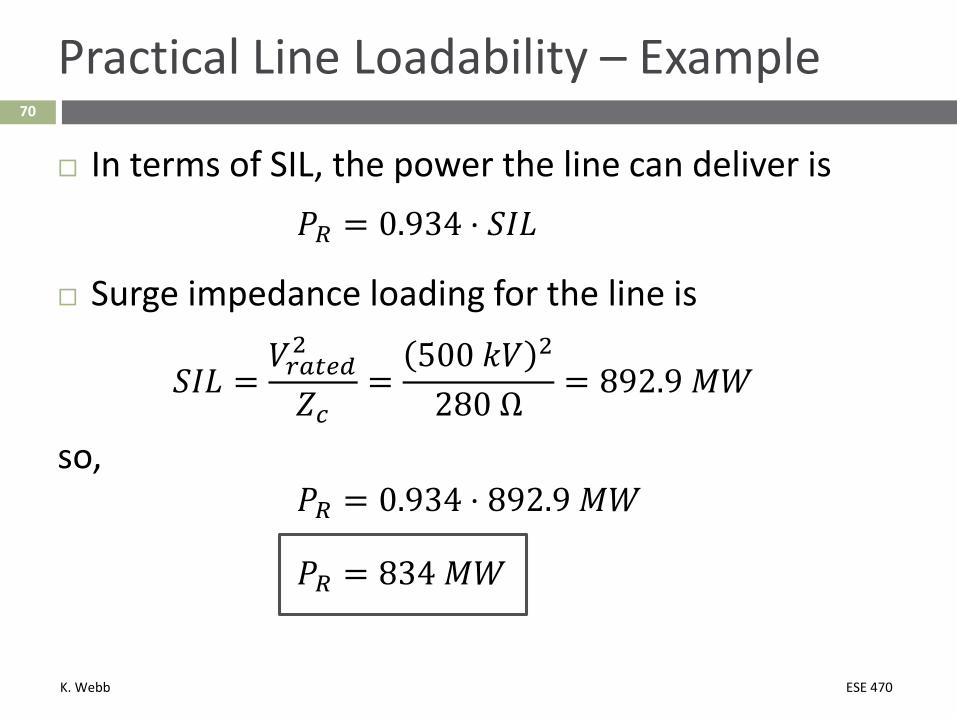
Practical Line Loadability – Example
In terms of SIL, the power the line can deliver is𝑃𝑃𝑅𝑅 = 0.934 ⋅ 𝑆𝑆𝐼𝐼𝜔𝜔
Surge impedance loading for the line is
𝑆𝑆𝐼𝐼𝜔𝜔 =𝑉𝑉𝑟𝑟𝑟𝑟𝑟𝑟𝑒𝑒𝑑𝑑2
𝑍𝑍𝑐𝑐=
500 𝑘𝑘𝑉𝑉 2
280 Ω= 892.9 𝑀𝑀𝑀𝑀
so,𝑃𝑃𝑅𝑅 = 0.934 ⋅ 892.9 𝑀𝑀𝑀𝑀
𝑃𝑃𝑅𝑅 = 834 𝑀𝑀𝑀𝑀

K. Webb ESE 470
Reactive Compensation71
K. Webb ESE 470
72
Reactive Compensation
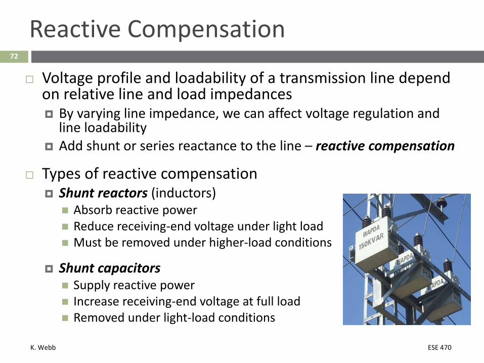
Voltage profile and loadability of a transmission line depend on relative line and load impedances By varying line impedance, we can affect voltage regulation and
line loadability Add shunt or series reactance to the line – reactive compensation
Types of reactive compensation Shunt reactors (inductors) Absorb reactive power Reduce receiving-end voltage under light load Must be removed under higher-load conditions
Shunt capacitors Supply reactive power Increase receiving-end voltage at full load Removed under light-load conditions

K. Webb ESE 470
73
Reactive Compensation
Types of reactive compensation (cont’d) Series capacitors Reduce series line impedance Reduce line voltage drops Increase steady-state stability limit
Static VAR compensators (SVCs) Thyristor-controlled shunt reactors and capacitors Automatically adjust compensation depending on load

K. Webb ESE 470
74
Reactive Compensation
Amount of reactive compensation is typically expressed as a percentage of line impedance
For example, the circuit above shows a transmission line with 𝑁𝑁𝜔𝜔% shunt reactive compensation

K. Webb ESE 470
75
Reactive Compensation – Example 5.9
Consider a 300 km, 765 kV, three-phase transmission line with the following chain parameters: 𝐴𝐴 = 0.93𝑗3∠0.𝑗09° 𝐵𝐵 = 𝑍𝑍′ = 9𝑗∠𝑗𝑗.𝑗° Shunt reactors, switched in during light-load conditions only,
provide 75% compensation Full-load current is 1.9 kA at 730 kV with unity power factor The sending-end voltage, 𝑉𝑉𝑆𝑆, is constant
Determine: %𝑉𝑉𝐼𝐼 of the uncompensated line %𝑉𝑉𝐼𝐼 of the compensated line

K. Webb ESE 470
76
Reactive Compensation – Example 5.9 Full-load, line-to-neutral, receiving-end voltage, using it as the 0° phase reference:
𝑽𝑽𝑅𝑅𝑅𝑅𝑅𝑅 =730
3∠0° 𝑘𝑘𝑉𝑉 = 421.5∠0° 𝑘𝑘𝑉𝑉
Use chain parameters to determine the sending-end voltage, 𝑽𝑽𝑆𝑆𝑽𝑽𝑆𝑆 = 𝐴𝐴𝑽𝑽𝑅𝑅𝑅𝑅𝑅𝑅 + 𝐵𝐵𝑰𝑰𝑅𝑅𝑅𝑅𝑅𝑅𝑽𝑽𝑆𝑆 = 0.93𝑗3∠0.𝑗09° (421.5∠0° 𝑘𝑘𝑉𝑉) + 9𝑗∠𝑗𝑗.𝑗° Ω 1.9∠0° 𝑘𝑘𝐴𝐴𝑽𝑽𝑆𝑆 = 442.3∠𝑗𝑗.𝑗° 𝑘𝑘𝑉𝑉
The no-load, line-to-neutral, receiving-end voltage is
𝑽𝑽𝑅𝑅𝑅𝑅𝑅𝑅 =𝑽𝑽𝑆𝑆𝐴𝐴
=442.3∠𝑗𝑗.𝑗° 𝑘𝑘𝑉𝑉0.93𝑗3∠0.𝑗09°
= 474.9∠𝑗𝑗.𝑗° 𝑘𝑘𝑉𝑉
Percent voltage regulation for the uncompensated line is
%𝑉𝑉𝐼𝐼 =𝑉𝑉𝑅𝑅𝑅𝑅𝑅𝑅 − 𝑉𝑉𝑅𝑅𝑅𝑅𝑅𝑅
𝑉𝑉𝑅𝑅𝑅𝑅𝑅𝑅⋅ 100% =
474.9 𝑘𝑘𝑉𝑉 − 421.5 𝑘𝑘𝑉𝑉421.5 𝑘𝑘𝑉𝑉
⋅ 100%
%𝑉𝑉𝐼𝐼 = 12.7%

K. Webb ESE 470
77
Reactive Compensation – Example 5.9
For the compensated line, we need to calculate new chain parameters
Shunt admittance of the uncompensated line can be determined from the known chain parameters
𝐴𝐴 = 0.93𝑗3∠0.𝑗09° = 1 +𝑌𝑌′𝑍𝑍′
2where
𝑍𝑍′ = 𝐵𝐵 = 9𝑗∠𝑗𝑗.2 ΩSo,
𝑌𝑌′ =𝐴𝐴 − 1 2𝑍𝑍′
=0.93𝑗3∠0.𝑗09° − 1 2
9𝑗∠𝑗𝑗.𝑗° Ω
𝑌𝑌′ = 1.418 × 10⁻³∠𝑗9.9𝑗° 𝑆𝑆
𝑌𝑌′ = 759 × 10−9 + 𝑗𝑗𝑗.42 × 10−3 𝑆𝑆

K. Webb ESE 470
78
Reactive Compensation – Example 5.9
After adding compensation, the equivalent shunt susceptance decreases by 75%
𝑌𝑌𝑒𝑒𝑒𝑒 = 759 × 10−9 + 𝑗𝑗𝑗.42 × 10−3 𝑆𝑆 ⋅ 0.25
𝑌𝑌𝑒𝑒𝑒𝑒 = 759 × 10−9 + 𝑗𝑗355 × 10−6 𝑆𝑆
Use 𝑌𝑌𝑒𝑒𝑒𝑒 to calculate the 𝐴𝐴 parameter for the compensated line
𝐴𝐴𝑒𝑒𝑒𝑒 = 1 +𝑌𝑌𝑒𝑒𝑒𝑒𝑍𝑍′
2= 0.9𝑗3∠0.05°
Note that shunt reactive compensation does not affect the series impedance, 𝑍𝑍𝑍, and therefor does not affect 𝐵𝐵

K. Webb ESE 470
79
Reactive Compensation – Example 5.9
The no-load receiving-end voltage for the compensated line:
𝑽𝑽𝑅𝑅𝑅𝑅𝑅𝑅 =𝑽𝑽𝑆𝑆𝐴𝐴𝑒𝑒𝑒𝑒
=442.3∠𝑗𝑗.𝑗° 𝑘𝑘𝑉𝑉
0.9𝑗3∠0.05°
𝑽𝑽𝑅𝑅𝑅𝑅𝑅𝑅 = 449.9∠𝑗𝑗.𝑗° 𝑘𝑘𝑉𝑉
Percent voltage regulation for the compensated line is
%𝑉𝑉𝐼𝐼 =𝑽𝑽𝑅𝑅𝑅𝑅𝑅𝑅 − 𝑽𝑽𝑅𝑅𝑅𝑅𝑅𝑅
𝑽𝑽𝑅𝑅𝑅𝑅𝑅𝑅⋅ 100%
%𝑉𝑉𝐼𝐼 =449.9 𝑘𝑘𝑉𝑉 − 421.5 𝑘𝑘𝑉𝑉
421.5 𝑘𝑘𝑉𝑉 ⋅ 100%
%𝑉𝑉𝐼𝐼 = 6.8%
Reactive compensation has improved voltage regulation from 12.7% to 6.8%