secondary stresses in bowstring timber trusses
TRANSCRIPT

Portland State University Portland State University
PDXScholar PDXScholar
Dissertations and Theses Dissertations and Theses
1983
Secondary stresses in bowstring timber trusses Secondary stresses in bowstring timber trusses
John F. Bradford Portland State University
Follow this and additional works at: https://pdxscholar.library.pdx.edu/open_access_etds
Part of the Civil Engineering Commons, and the Structural Engineering Commons
Let us know how access to this document benefits you.
Recommended Citation Recommended Citation Bradford, John F., "Secondary stresses in bowstring timber trusses" (1983). Dissertations and Theses. Paper 3252. https://doi.org/10.15760/etd.3242
This Thesis is brought to you for free and open access. It has been accepted for inclusion in Dissertations and Theses by an authorized administrator of PDXScholar. Please contact us if we can make this document more accessible: [email protected].

AN ABSTRACT OF THE THESIS OF John F. Bradford for the Degree of Master
of Science in Applied Science (Structural Engineering) presented Feb-
ruary 21, 1983.
Title: Secondary Stresses in Bowstring Timber Trusses.
F
Civil Engineering
This study was undertaken in order to determine analytically the
magnitude of the secondary (i.e., joint deflection induced) moments in
the continuous glued-laminated chords of bowstring timber trusses.
Traditionally, these moments have been assumed to be small and therefore
neglected. The American Institute of Timber Construction makes no men-
tion of these moments in their recommended design procedure.

The results of the investigation show, however, that these mo
ments are theoretically very large--considerably larger than the pri
mary moment. In a typical design problem, a truss designed neglecting
the secondary moments was found to be 36% overstressed when these mo
ments were considered.
2
Proposed design charts and characteristic equations which repre
sent the secondary moments are presented for three truss configurations.
A byproduct of the investigation was the development of a method
to produce general characteristic equations for a specific structural
configuration. These equations allow the designer to quickly determine
the maximum moments, shears, deflections or other variables which may
be affected by changing a parameter such as the moment of inertia of
one of the members. The effect on the structure of changing a parame
ter can be determined immediately by the use of the characteristic equa
tions as opposed to the significant time and effort involved in running
a complete frame analysis. The technique is primarily intended for
standard structures, such as trusses, but might also be useful for
structures which require a large number of iterations before obtaining
the final design.
A computer program for the technique which can be implemented on
a small microcomputer is presented.

SECONDARY STRESSES
IN BOWSTRING TIMBER TRUSSES
by
JOHN F. BRADFORD
A thesis submitted in partial fulfillment of the requirements for the degree of
MASTER OF SCIENCE in
APPLIED SC !ENCE (STRUCTURAL ENGINEERING)
Portland State University 1983

TO THE OFFICE OF GRADUATE STUDIES AND RESEARCH:
The members of the Committee approve the thesis of John F.
Bradford presented February 21, 1983.
Engineering
APPROVED:
Franz N. Rad, Department of Civil Engineering
Stanl~ E. Rauch, Dean of Graduate Studies and Research

TO MY LOVING WIFE
DONETA
and
MY FOUR CHILDREN
JOSHUA
KAYLA
LARISSA
MEGAN

ACKNOWLEDGEMENTS
This investigation was carried out under the supervision of
Dr. Franz N. Rad. The author is indebted to Dr. Rad for his help and
advice throughout this work.
The author would also like to thank the other members of his
thesis conmittee, Dr. Hacik Erzurumlu, Dr. M. M. Gorji, and Dr. Phil
J. Gold for their helpful connnents and suggestions.
The author would like to thank Mr. Dick W. Ebeling for his
valuable input and for allowing the author to devote a considerable
number of office hours to this work.
Thanks are also due to Dr. Wendelin H. Mueller for his assist
ance in the application of the frame analysis program, "RIGID", which
he authored; also to Leon Kempner for his assistance in the application
of the SAPIV program.
The author would like to extend his thanks to Mrs. Sharon Ull- .
rich for the excellent typing of this thesis.
I am especially indebted to my dear and loving wife and to my
four children for their understanding, encouragement and patience
throughout the author's graduate work.

TABLE OF CONTENTS
PAGE
ACKNOWLEDGEMENTS • • • • • • • • • • • • • • • • • • • • • • • • • • iv
LIST OF TABLES • . . . . . . . . . . . . . . . . . . . . . . . . . . ix
LIST OF FIGURES xii . . . . . . . . . . . . . . . . . . . . . . . . . . NOTATION •••• . . . . . . . . . . . . . . . . . . . . . . . . . . xvi
CHAPIER
I INTRODUCTION • • • • • • • • • • • • • • • • • • • • • • • 1
II
III
1.1 BACKGROUND. . . . . . . . . . . . . . . . . . . . 1.2 DESIGN METHODS. . . . . . . . . . . . . . . . . . . .
1.2.l Traditional Method . . . . . . . . . . . 1.2.2 Computer Frame Analysis. . . . . . . . . . . .
1.3 DESIGN PROBLEMS . . . . . . . . . . . . . . . . . . . 1.4 SCOPE OF THIS INVESTIGATION . . . . . . . . . . . . . STRUCTURAL CHARACTERISTICS AND CONSTRUCTION DETAILS OF GLUED-LAMINATED BOWSTRING TRUSSES • • • • • • • • . . . 2.1 STRUCTURAL CHARACTERISTICS. . . . . . . . . . . . . . 2.2 CeJ.iMON CONSTRUCTION DETAILS • • • • • • • • • • • • •
2.2.1 Geometry . . . . . . . . . . . . . . . . . . . 2.2.2 Details. . . . . . . . . . . . . . . . . . . .
COMPUTER MODELS ••••• . . . . . . . . . . . . . . . . . 3.1 GENERAL INFORMATION . . . . . . . . . . . . . . . . . 3.2 EIGHT PANEL TRUSS • . . . . . . . . . . . . . . . . .
1
2
2
3
4
5
7
7
8
8
10
16
16
16

IV
3.3
3.4
vi
PAGE
3.2.l Model I. • • • • • • • • • • • • • • • • • • • 16
3.2.2
3.2.3
3.2.4
3.2.5
Model II • . . . . . . . . . . . . . . . . . . 17
Model III. . . . . . . . . . . . . . . . . . . 17
Loading •• • • • • • • • • • • • • • • • • • • 20
Variations • • • • • • • • • • • • • • . . . . 20
3.2.5.l Web Connection Bolt Slippage. • • • • 20
3.2.5.2 Heel Joint Slippage • • • • • • • • • 22
3.2.5.3 Heel Joint Fixity • • • • • • • • • • 22
3.2.5.4
3.2.5.5
3.2.5.6
3.2.5.7
Bottom Chord Splice Bolt Slippage
Bottom Chord Splice Fixity ••••
Heel Plate Fixity, Chord Rotation Permitted at Bolts ••••••••
• •
. . • •
Combinations of Effects • • • • • • •
22
23
23
23
3.2.6 Member Properties. • • • • • • • • • • • • • • 23
TEN PANEL TRUSS • • • • • • • • • • • • • • • • • • • 27
TWELVE PANEL TRUSS. . . . . . . . . . . . . . . . . . 27
PRil1ARY MOMENTS IN THE TOP CHORD . . . . . . . . . . . . . 30
4.1 METHODS OF ANALYSIS • • • • • • • • • • • • • • • • • 30
4.1.1 AITC Method. • • • • • • • • • • • • • • • • • 30
4.1.2 Moment Distribution. • • • • • • • • • • • • • 31
4.1.2.l FEM due to "Pe" • • • • • • • • • . . 31
4.1.2.2 FEM due to External Member Loads. • • 31
4.1.2.3 Moment Distribution . . . . . . . . . 32
V SECONDARY MC11ENTS IN THE BOTTOM CHORD. • • • • • • • • • • 46

vii
PAGE
5 .1 PARAMETERS AFFECT ING THE SECONDARY MCMENT IN THE BarTOM CHORD. • • • • • • • • • • • • • • • • • • 46
5.2 ~C AS A FUNCTION OF ~C- • • • • • • • • • • • • • • 52
5.3 THE EFFECT OF ~c ON ~c· •••••
5.4 ~c AS A FUNCTION OF A.re AND 1tc· •
• • • • • • • • • 54
. . . . . . • • • 60
5. 5 THE EFFECT OF 1tc ON THE MCMENT IN 'i'HE BOTTOM CHORD • 6 7
5.6 INFLUENCE OF TRUSS SPAN (L) ON ~c· • • • • • • • • • 71
5.7 THE INFLUENCE OF LOADING ON ~C ••••••••••• 75
5. 8 THE INFLUENCE OF THE NUMBER OF PANELS ON ~C. • • • • 7 5
5.9 s~ • • • • • • • • • • • • • • • • • • • • • • • 79
VI SECONDARY MOMENTS IN THE TOP CHORD . . • • • • • • • • • • 83
6 .1 PARAMETERS AFFECTING M.rc ••••••• • • • • • • • • 85
6.2 DEVELOPMENT OF EQUATIONS •• . . . . . . . . . . . 85
VII VERIFICATION OF EQUATIONS DEVELOPED IN CHAPTERS V AND VI • 98
VIII OTHER FACTORS AFFECTING THE SECONDARY MCMENTS IN THE CHORDS • • • • • • • • • • • • • • • • • • • • • • • • • • 102
8.1 BOLT SLIPPAGE IN THE WEB CONNECTIONS •• • • • . . . • 102
8. 2 HEEL FIXITY • . . . . . . . . . . . . . . . . . . . • 103
8.3 BOLT SLIPPAGE IN THE HEEL CONNECTION. • • • • • • • • 104
8.4 BOTTOM CHORD SPLICE • • • • • • • • • • . . . . . • • 108
8.5 TERTIARY (P-6.) MCMENTS • . . . . . . . . . . • • 108
IX DEVELOPMENT OF A SYSTEMATIC APPROACH TO THE DESIGN OF STANDARD STRUCTURES • • • • • • • • • • • • • •
9.1 INTRODUCTION. • • • • • • • • • • • • • • •
. . . • 110
• • • 110
9.2 GENERAL CHARACTERISTIC EQUATION CONCEPT • • • • • • • 110
viii
PAGE
9. 3 PARAMETERS TO BE VARIED • • • • • • • • • • • . • • • • 114
9.4 DEVELOPMENT OF A GENERAL CHARACTERISTIC EQUATION ••• 115
9.4.1 Sunnnary •••••••••••••• • • • • • • 119
9.5 COMPUTER rnPLEMENTATION OF THE PROCEDURE •• • • • • • 122
9.6 EXAMPLE PROBLEM • • • • • • • • • • . . . . . . . . . 123
9.6.1 I. Data Base Preparation. . . . • • • • • • • 123
9.6.2 II. Development of the Characteristic Equations •••••••••••••• . . . . . 124
9.6.3
9.6.4
III.A. Verification of Equations •• • • • • • 127
III.B. Design Procedure ••••••• . . . . 131
X OBSERVATIONS . . . . . • • • • • • • • . . . . . . • • • • 138
10.1 EXAMPLE PROBLEM • • • • • • • • . . • • • • • • • • • 138
10.2 DESIGN OPT1MIZATION • . . • • . . . . • • • . . . . . 143
10.3 THE EFFECT OF THE SECONDARY MOMENTS ON THE WEBS ••• 144
XI SUMMARY, CONCLUSIONS AND RECOMMENDATIONS • . . . • • • • • 145
11.1 SUMMARY ••• • • . . . . . . . . . . . . . • • 145
11. 2 CONCLUSIONS • • . . • • • • • • • • • • . . . . . . • 146
11.3 RECCJ1MENDATIONS • • • • • • . . . . . . . . . • • • • 147
APPENDIX 1
APPENDIX 2
APPENDIX 3
APPENDIX 4
REFERENCES ••
DERIVATION AND JUSTIFICATION OF FIXED END MCMENT EQUATIONS FOR THE PRIMARY MOMENT ANALYSIS • • • • • •
SUMMARY OF THE FRAME ANALYSIS COMPUTER DATA • • . . . 148
163
"PINNED MEMBER" DESIGN METHOD • • • • • • • • • • • • 169
"GENERAL CHARACTERISTIC EQUATION" METHOD COMPUTER PROO~. • • • • • • • • • • • • • • • • • • • • • • 171
• • • • • • • • • • • • • • • • • • . . . . . • ••• 178
LIST OF TABLES
TABLE PAGE
3.1
3.2
4.1
Design Values for Structural Glued Laminated Timber
Combination No. 3. AITC 117-79 ••••• • • • . . . . . . Section Properties of Chord Members • . . . . . . . . . . Moment Distribution for the 8 Panel Truss • . . . . • • •
4.2 Primary Moments in the Top Chord of a 100 Ft., 8 Panel
25
26
37
Truss with lK/Ft. Loading (Obtained from Eq. 4.6 and 4.7) 38
4.3 8 Panel Truss - Primary Moments in the Top Chord Obtained
4.4
4.5
4.6
from Computer Results • • • . . . . . . . . • • • . . . . Moment Distribution for the 10 Panel Truss •• . . . . . . Primary Moments in the Top Chord of a 100 Ft., 10 Panel
Truss with lK/Ft. Loading (Obtained from Eq. 4.6 and 4.7)
Moment Distribution for the 12 Panel Truss •••• . . . . 4.7 Primary Moments in the Top Chord of a 100 Ft., 12 Panel
38
40
41
43
Truss with lK/Ft. Loading (Obtained from Eq. 4.6 and 4.7) 44
5.1 Principal Parameters Affecting the Secondary Moments in
the Bottom Chord. • • • • • • • • • • • • • • • • • • • •
5.2 Computation of ~ and CB for the Eight, Ten and Twelve
5.3
5.4
5.5
Panel Trusses using Eq. 5.4 and 5.5 • • • • . . . . . . . Computation of N •• . . • • • • • • • • • • • • • • • • •
Computation of MBC using Eq. 5.11 ••••••••••••
Computation of ~l and CBl using Eq. 5.14 and 5.15 ••••
47
53
56
61
65

x
PAGE
5.6 Computation of ~l using Eq. 5.16 • • • • • • • • • • • • 65
5.7 Computation of kB2
, cB2 and ~2 using Eq. 5.19, 5.20 and
s.21 •••• • • • • • • • • • • • • • • • • . . • • . . . 5.8 Computation of ~2 using Eq. 5.22 ••••••••••••
72
72
5.9 Data for Fig. 5.9 and Computation of ~S' CBS and ~5 • • 77
5.10
5.11
5.12
6.1
Computation of KB5 •••••••••••••• • • • • 79
Summary of General Equations for the Bottom Chord Second-
ary Moments • • • • • • • • • • • • • • • • • • • • • • • 80
Sunnnary of Explicit Equations for the Bottom Chord Sec-
ondary Moments. • • • • • • • • • • • • • • • • • • • • • 82
General Equations for the Top Chord Secondary Moment. • • 87
6.2 Computation of ~ and CT for an 8 Panel Truss using Eq.
6.3 and 6.4 . . . . . • • • • • • • • • • • • • • • • • • 89
6.3 Computation of k.ro' CTO and &ro for an 8 Panel Truss
using Eq. 6.6, 6.7, 6.8 and 6.9 • • • . • • • • • • • • • 89
6.4 Computation of k.rl and CTl for an 8 Panel Truss using Eq.
6. 11 and 6. 12 • • • • • • • • • • • • • . • • • • • . • . 90
6.5 Computation of ~2 , CT2 and ~2 for an 8 Panel Truss
using Eq. 6.14, 6.15, 6.16 and 6.17 • • • • • • • • • • • 90
6.6 Computation of kTS' cT5 and ~S for an 8 Panel Truss
using Eq. 6.21, 6.22, 6.23 and 6.24 • . • • . • • • • • • 90
6.7 Explicit Equations for the Secondary Moment in the Top
Chord • • • • • • • • . • • • . • • . • • • . . • . • • • 91
6.8 Calculated Data for Curve of Fig. 6.1 using Equations
from Table 6.7. • • • • • • • • • • • • • • • • • • • • • 91

xi
PAGE
6.9 Calculated Data for Fig. 6.2 Based on the Equations
6.10
6.11
6.12
7.la
7.lb
8.1
9.1
from Table 6.7. • • • • • • • • • • • • • • • • • • • • •
Calculated Values of ~1 ••• • • • • • • • • • • • • • •
Calculated Values of K.r 2• ••• • • • • • • • • • • • • •
Calculated Values of ~s· •• • • • • • • • • • • • • • •
Verification Data • • • • • • • • • • • • • • • • • • • •
Verification Data • • • • • • • • • • • • • • • • • • • •
Effect of Bolt Slippage in the Web Connections. • • • • •
Parameter Data for Example Problem. • • • • • • • • • • •
9.2 Output Data for the Chosen Variables (Obtained from the
92
92
93
95
100
101
103
123
Computer Frame Analysis) ••••••••• • • • • • • • • 125
9.3 Constants for the "General Characteristic Equations" for
the Bowstring Truss Example Problem • • • • • • • • • • • 128
9.4 General Characteristic Equation Verification Data • • • • 130
A2.l Data for Figure 5.1 • • • • • . • • • • • • • • • • • • • 164
A2.2 Computer Frame Analysis Data. • • • • • • • • • • • • • • 165
A2.3a Computer Frame Analysis Data Used to Plot Fig. 6.la • • • 167
A2.3b Computer Frame Analysis Data Used to Plot Fig. 6.lb • • . 168

FIGURE
2.1
2.2
LIST OF FIGURES
Truss configurations considered • • • • • • • • • • • • •
Alternate web configuration • • • • • . . . . . . . . . .
PAGE
9
9
2.3 8 panel truss geometry. • • • • • • • • • • • • • • • • • 11
2.4 10 panel truss geometry • • • • • • • • • • • • • • • • • 12
2.5
2.6
2.7
12 panel truss geometry • • • • • • • • • • • • • • • • •
Concentric heel connection. • • • • • • • • • • • • • • •
Eccentric heel connection • • • • • . . • • • • • • • • •
13
14
14
2.8 Typical web connection. • • • • • • • • • • • • • • • • • 15
2.9
3.1
3.3
3.4
3.5
3.6
4.1
Typical bottom chord splice
8 panel - Model I ("RIGID")
. . . . . • • • • • • • • • •
• • • • • • • • • • • • • • •
8 panel - Model II (SAP IV) • • • • • • • • • • •
8 panel truss - Model III ("RIGID" - Full Truss).
Fixed heel with rotation of bottom chord at bolts
• • • •
. . . . • • • •
10 panel - Model I ("RIGID"). • • • • • • • • • • • • • •
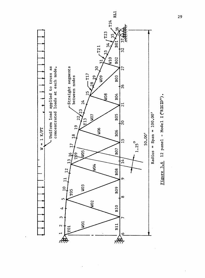
12 panel - Model I ("RIGID"). • • • • • • • • • • • • • •
Fixed end forces on a top chord panel due to 'P x e'. • •
4.2 Fixed end forces on a top chord panel due to a concentra-
ted load. • • • • • • • • • • • • • • • • • • • • • • • •
4.3 Free-body forces on a top chord segment . • • • • • . • •
4.4 8 panel truss - primary moment data • • • • • • • • • • •
4.5 Primary moment diagram for a 100 ft. span 8 panel truss
one kip per foot. • • • • • • • • • • • • . • • • • • • •
15
18
19
21
24
28
29
33
33
34
39
39

xiii
PAGE
4.6 10 panel truss - primary moment data. • • • • • • • • • • 42
4.7 Primary moment diagram for a 100 ft. span 10 panel truss
4.8
4.9
s.1
5.2a
5.2b
5.2c
5.3a
5.3b
5.3c
5.4a
5.4b
5.4c
one kip per ft. • • • • • • • • • • • • • • • • • • • • • 42
12 panel truss - primary moment data. • • • • • • • • • • 45
Primary moment diagram for a 100 ft. span 12 panel truss
one kip per ft. • • • • • • • • • • • • • • • • • • • • • 45
Typical bottom chord secondary moment diagrams. • • • • • 48
8 panel truss - secondary moment in the bottom chord as a
function of ~e and ~e • • • • • • • • • • • • • • • • • 49
10 panel truss - secondary moment in the bottom chord as
a function of ~e and ~e • • • • • • • • • • • • • • • • 50
12 panel truss - secondary moment in the bottom chord as
a function of ~e and ~e • • • • • • • • • • • • • • • • 51
8 panel truss - secondary moment and bending stress in
the bottom chord as computed from Equation 5.11 •• . . . 57
10 panel truss - secondary moment and bending stress in
the bottom chord as computed from Equation 5.11 • • • • • 58
12 panel truss - secondary moment and bending stress in
the bottom chord as computed from Equation 5.11 • • • • • 59
8 panel truss - secondary moment in the bottom chord as a
function of A.re and 1Te • • • • • • • • • • • • • • • • • 62
10 panel truss - secondary moment in the bottom chord as
a function of Arre and ~e • • • • • • • • • • • • • • • • 63
12 panel truss - secondary moment in the bottom chord as
a function of Arre and I.re • • • • • • • • • • • • • • • • 64
xiv
PAGE
5.5
5.6
~l - Adjustment factor to ~C for variation in A.re • • • Secondary moment in the bottom chord as a function of ~C
5.7 Effect of secondary moment in the chords on the axial
forces in the members • • • • • • • • • • • • • • • • • •
5.8 ~2 - Adjustment factor to ?\c to account for variations
in I.re· • • • • • • . • • • • • • • • • • • • • • • • • •
5.9 Secondary moment in the bottom chord as a function of the
number of panels in the truss • • • • • • • • • • • • • •
5.10 KB5
- Adjustment factor to ?\c to account for a varying
number of panels in the truss • • • • • • • • • • • • • •
6.1 Top chord moment diagrams for typical cases • . . . . . . 6.2 8 panel truss - secondary moment in the top chord as a
66
68
69
73
76
78
84
function of 1'rc and J7c • . • • • • • • • • • • • • • • . 94
6.3 8 panel truss - secondary moment and bending stress in
the top chord as computed from Equations 6.2 and 6.5. • • 95
6.4 ~l - Adjustment factor to ~C to account for variation
in ~c· • • • • • • • • . • • • . • • • • • • • . • • . • 96
6.5 KT2 - Adjustment factor to ~c to account for variation
in ~c· • • • • . • • • • • • • • • . . • • • • • • • . • 96
6.6 ~5 - Adjustment factor to M.rc to account for a variation
in the number of panels in the truss ••• • • • • • • • • 97
8.1 Probable stress distribution in an eccentric heel • • • • 105
8.2 Amplification of moment in the bottom chord due to an
eccentric heel. • • • • • • • • • • • • • • • • • • • • • 105

xv
PAGE
B.3 Effect of a fully fixed heel on the bottom chord moment
in an 8 panel truss with bolt slippage permitted in the
Al.l
Al.2
Al.3
Al.4
Al.5
web connections ••• • • • • • • • • • • • • • • • • • • 106
Fixed end forces in a top chord panel • • • • • • • • • • 149
Free-body forces on a top chord segment under fixed end
conditions ••••• • • • • • • • • • • • • • • • • • • • 149
Model and nomenclature used by Roark and Young. • • ••• 153
Data for Example Al.l ••• • • • • • • • • • • • • • • • 160
Load components for Example Al.l •• • • • • • • • •••• 160
NOTATION
a • • • • • • • • Reference dimension for locating a concentrated load
on a chord segment.
a' • • • • • • • • Intermediate coefficient used in the development of
primary moments.
b • • • • • • • • Reference dimension for locating a concentrated load
on a chord segment.
I b •••••••• Intermediate coefficient used in the development of
primary moments •
c • • • • • • • • Cos 9.
e • • • . . . . • Eccentricity of the top chord between panel points,
Ft.
f ( ) • . . • • • • A function of ••• (expression).
~· ••••• Constant used in equation to define ~co•
~i ••••••• Constant used in equation to define KBi' an adjust-·
ment factor for the characteristic equation for the
bottom chord as developed in Chapter v.
&ri ••••••• Constant used in equation to define I<Ti' an adjust
ment factor for the characteristic equation for the
top chord as developed in Chapter VI.
gijJ • • • • • • Constant used in the general characteristic equation
to define an adjustment factor to account for the
effect of the ith parameter on the jth variable under

xVii
load case f... j •••••••• Subscript to represent the jth variable (i.e., maxi-
mum bottom chord moment, etc.).
kB. • • • . • • • Constant used in equation to define ~co·
kBi • . • • • • • Constant used in equation to define KBi' an adjust-
ment factor for the characteristic equation for the
bottom chord as developed in Chapter V.
k.ri ••••••• Constant used in equation to define ~i' an adjust
ment factor for the characteristic equation for the
top chord as developed in Chapter VI.
k .. 0 l.J ,k
. . . . . . Constant used in the general characteristic equation
to define an adjustment factor to account for the
effect of the ith parameter on the jth variable under
load case 9..
J. • • • • • • • • Subscript to represent the .R th load case.
n • • • • • . . . The total number of parameters (i.e., area of bottom
chord, etc.).
p •••••••• Virtual load.
qBi ••••••• Intermediate factor used to develop gBi•
s • • • • • • • • Sin Q.
w •••••••• Uniform load on the top chord.
B w • • • • • • Base value of w used to compute ~O and CBo•
••••••• The value of a parameter (such as ~c>•
• •
x •
x .• l. • • • • • • • The value of the ith parameter.
(=lK/ft).
xii • • • • • • • The lower limit of the ith parameter used to develop
the general characteristic equation.

xviii
xi2
• • • • • • • The base value of the ith parameter used to develop
the general characteristic equation.
xi3
• • • • • • • The upper limit of the ith parameter used to develop
the general characteristic equation.
y •••••••• The value of a variable (such as MBe) •
y .•• J
• • • • • • The value of the jth variable.
A • • • • • • • • Area of a member, sq. in.
~e • • • • • • • Area of the bottom chord, sq. in.
B ABe ••••••• Base value of ~e·
~e ••••••• Area of the top chord, sq. in.
B Ate • •••••• Base value of A.re·
B • • • • • • • • Intermediate coefficient used to define g.
B •. n 1.J~
• •
• •
. . • •
• • • •
Value of B for case ij/.
Intermediate coefficient used in the development of
primary moments.
BHH • • • • • • • Intermediate coefficient used in the development of
primary moments.
BHM • • • • • • • Intermediate coefficient used in the development of
primary moments.
BHV • • • • • • • Intermediate coefficient used in the development of
primary moments.
BMH. • . . • • • • Intermediate coefficient used in the development of
primary moments.
BMM • • • • • • • Intermediate coefficient used in the development of

x-ix
primary moments.
BMV • • • • • • • Intermediate coefficient used in the development of
primary moments.
BW • • • • • • • Intermediate coefficient used in the development of
primary moments.
BVM • • • • • • • Intermediate coefficient used in the development of
primary moments.
BVV • • • • • • • Intermediate coefficient used in the development of
primary moments •
BC •• • • • • • • Bottom chord of the truss - used as a subscript.
CB •••••••• Constant used in equation to define ~co•
CBi ••••••• Constant used in equation to define ~i' an adjust-
ment factor for the characteristic equation for the
bottom chord as developed in Chapter v.
CT •••••••• Constant used in equation to define ~co•
CTi ••••••• Constant used in equation to define K.ri' an adjust-
ment factor for the characteristic equation for the
top chord as developed in Chapter VI.
C .. n •••••• Constant used in the general characteristic equation 1J,A
to define an adjustment factor to account for the
effect of the ith parameter on the jth variable under
load case j.
co •• • • • • • • Carry over factor for moment distribution method.
DF •• . . . . • • Distribution factor for moment distribution method.
DFL • • • • • • • Douglas Fir/Larch.
E • • • • • • •• Modulus of elasticity, psi.

Fb x-x • • • • • • Allowable bending stress about the x-x axis.
Fe •• • • • • • • Allowable compression stress.
Ft •• • • • • • • Allowable tension stress.
FEM • • • • • • • Fixed end moment.
FEMA (Pe) •• • •
I • • • • • • •
~c •••• • •
B 1Bc • I.re •
• • • • •
• • • • •
~c • • • • • •
• Fixed end moment at point A produced by an axial
load acting on a curved member.
M f i . . 4 • oment o nert1a, in •
• Moment of inertia of the bottom chord, in4
•
• Base value of 1ac• • Moment of inertia of the top chord, in4 •
• Base value of ~c·
xx
K • • • • • • • • Member stiffness factor used in the moment distribu-
tion method of analysis.
~i • • • • • • • Adjustment factor to the moment in the bottom chord
to account for variation in parameter i.
~i • • • • • • • Adjustment factor to the moment in the top chord to
account for variation in parameter i.
L • • • • • • • • Span length of truss, ft.
12 •• • • • • • • Material grade for Lam stock.
L2D • • • • • • • Dense grade of L2 Lam stock.
LFH ••••••• Load factors used in developing the primary moment
equations--as defined by Roark and Young, Formulas
for Stress and Strain, Fifth Edition.
LFM • • • • • • • Load factors used in developing the primary moment
equations--as defined by Roark and Young, Formulas

for Stress and Strain, Fifth Edition.
LFV ••••••• Load factors used in developing the primary moment
equations--as defined by Roark and Young, Formulas
for Stress and Strain, Fifth Edition.
. . . . • • Moment at point i.
~c •••• • • • Maximum moment in the bottom chord, located at the
first panel point from the end of the truss.
xxi
~co• •••••• Value of ~C when all parameters are at base values
except ~c·
•• Base value of ~c·
. . . • Maximum moment in the top chord, located at the
first panel point from the end of the truss.
M.rco· •••••• Values of ~C when all parameters are at base values
except ~c·
N • • • • • • • • Power coefficient used in Chapter V to correlate the
effect of IBC on ~c·
NP. . . . . . • • Number of panels in the truss.
p • • • • . . . • Axial force in a member.
Q •• l. • • • • . . . Intermediate coefficients used in the development of
primary moments.
R • • • • • • • • Radius of the top chord (center line), ft.
VA •••••••• Shear at point A.
Wl •• • • • • • • Web number 1.
y .• J • • • • ••• Final value of the jth variable (such as ~C),
accounting for the chosen values of all parameters.
B Yj •••••••• Value of Yj using base values for all parameters.

xx ii
Y. /J • • • • • • • Value of Y. for load case R • J.A J
51
• • • • • • • • (DELTA) Tangential deflection of the roller support
of an arch section (see Fig. Al.3).
~ • • • • • • • • (ETA) Angle measured from the vertical line through
the centroid of the top chord radius of the truss to
the center of the top chord segment being considered.
~ • • • • • • • • (LAMBDA) Horizontal projection of a top chord panel
length, ft.
f • • • • • • • • (RHO) Radius of curvature of a member subjected to
bending.
0 • • • • • • • • (PHI) Angle measured from the upper end of a top
chord segment to the point i on the top chord.
t . . . . . . . . (PSI) Vertical projection of a top chord panel
length, ft.
~- • • • • • . . (DELTA) Joint deflection.
Q • • • . . . . . (THETA) One half of the included angle formed by the
arc of a top chord panel.
• • • • • • • (PI) Sequential Product operator.
• • • • • • • (SIGMA) Sequential Summation operator.
BP. • • • • • • • Eight panel truss.
lOP • • • • • • • Ten panel truss.
12P • • • • • • • Twelve panel truss.
01TC23 •••••• Designation assigned to the frame analysis computer
runs were the 0 indicates that ~c=A0 (see Table 3.2),
the 1 indicates IBC=I1
, TC2 indicates ~c=A2 , and 3

xx iii
indicates that ~c=I3 •
CHAF'.CER I
INTRODUCTION
1.1 BACKGROUND
The bowstring truss is a truss with a curved top chord, located
so that it follows the force line of an arch with the bottom chord act
ing as the tie. The webs of the truss are required only to provide
stability and to distribute concentrated and unbalanced loads which im
part substantial bending into an arch. The webs carry very small
forces which results in a very efficient truss, particularly for uni
form loads such as roof loads.
The early designs, used for many years, used three basic
methods to form the top chord. One method used dimension lumber re
sawn on one edge to the curved shape. The pieces were lapped approxi
mately one half of their length which resulted in a semi-continuous
segmented top chord--thus the term "segmental chord" bowstring was used
to describe these trusses.
A second method used small dimension lumber (2x4 or 2x6's) nail
laminated into a continuous curved chord with staggered butt splices
between pieces. They were sometimes built with one or two wider lami
nations to provide a ledger for the roof joists. The most common name
for this type of truss was the "Summerbell" truss.

The third method used large members resawn to a radius and butt
spliced at web joints. They were usually called "monochord" trusses.
With the advent of glued laminated timber (glu-lam) 1 engineers
began designing the trusses using truly continuous curved glu-lams for
the chords. The analysis of these trusses continued to assume "pin
jointed" members, recognizing the continuity of the chords only to re
distribute the already small primary bending moments.
1.2 DESIGN METHODS
Currently, two methods are known to be used in the industry to
analyze these trusses: the method mentioned above which will be re
ferred to as the traditional method; and by the use of a relatively
large capacity computer to perform a "frame analysis".
1.2.l Traditional Method
Traditionally, the most conunon method involves modeling the
truss assuming pinned joints and straight top chord segments between
panel points. A graphical technique known as the Maxwell diagram(l)
2
is normally used to compute member forces. Small microcomputers or
even progranunable calculators may also be used to compute member forces
using matrix or joint analysis techniques.
The moments in the top chord are computed using semi-empirical
equations such as those found in the AITC Timber Construction Manual~Z)
These equations use superposition to combine continuous beam moments
with moments induced by the eccentricity of the curved chord ('Pe'
effects). This moment is assumed to be distributed in the same manner

3
as the moment produced by the vertical loads.
Traditionally, secondary bending stresses induced by the deflec
tion of the truss have been ignored. Thus, the bottom chord has been
designed for pure tension (except when ceiling or other loads are ap
plied directly to the bottom chord). The top chords are designed using
the axial load and moments as described above.
The assumption has been that the secondary stresses are rela
tively small and therefore not worth the fairly large effort required
to compute them. As will be demonstrated in this study, however, the
secondary stresses may indeed be quite large. In a few cases investi
gated, the top chord moment at the critical location was found to be
several times larger than the primary moment, with the total bending
stress exceeding 60% of the stress allowed for pure bending. Previous
ly they were usually computed to be less than 10% when neglecting the
secondary stress. The result is that trusses designed by this method
may actually be overstressed by as much as 50% in some cases.
1.2.2 Computer Frame Analysis
The second method utilizes relatively large computers to ana
lyze the truss using a conventional matrix displacement frame analysis,
or a finite element analysis program. This method, therefore, does
take into account the effects of the "secondary" moments.
The "secondary" moments as referred to here are actually pri
mary moments in frame analysis, i.e., moments caused by joint deflec
tion. What would be called "secondary" moments in frame amalysis ter
minology (i.e., P- ~effect) will be denoted as "tertiary" moments here.

1.3 DESIGN PROBLEMS
To accurately model the curved chord of the truss the chord
must be broken up into several segments between each panel point. As
a result, a typical truss will have over 100 members in the model.
This poses several problems. Extensive time is required for model
development and data input. The coordinates of the top chord segments
must be accurately computed and correctly entered. This is a tedious
task which lends itself to errors. A minor error in coordinate input
can have drastic effects on the top chord moments.
4
The input of the loads is also a laborious task. Due to the
curvature, the horizontal projection of the members is different for
each member. Every joint in the top chord must therefore have the load
computed and input separately. The task of considering multiple load
cases, such as unbalanced loading which is critical for the design of
the webs in bowstring trusses, increases the task considerably.
These problems can be reduced by the use of a sophisticated pro
gram which has cylindrical coordinate and load generation capabilities.
Use of a small 8-bit microprocessor for such a task would be un
duly cumbersome, time consuming, and indeed impossible without a sophis
ticated program utilizing a mass storage device for storing the large
matrices. Matrix partitioning techniques would be required to manipu
late these large matrices. Programs of this sophistication are not
readily available for 8-bit machines. Even if a program were avail
able, the accuracy would be highly suspect for a structure with such
small member offsets.
5
Programs with these capabilities do exist for use on several
minicomputers. However, these machines (and the software) are much
more expensive than the smaller machines and are not found in most
small design firms. Even with such a system, or a large inhouse time
shared system, the time element and its associated cost is restrictive,
especially if the job has only a few trusses of a specific design.
In addition to design office practicality problems of the com
puter analysis method, the analysis itself can be misleading and the
degree of accuracy may be unjustified. As will be seen later in the
study, several factors such as bolt slippage can have a major effect
on the induced moments. With the type of web connection normally used
in these trusses (strap and pin), bolt slippage is highly probable. A
small amount of bolt slippage in the web connections can reduce the mo
ments in the chords by as much as 50%.
In light of this and the highly unpredictable nature of loading
and strength of the member, it seems unnecessary and indeed undesirable
to require an analysis of such "precision". As mentioned previously,
however, the secondary moments are substantial and should be accounted
for by some method of reasonable accuracy, even if the method results
in "overly precise" answers.
1.4 SCOPE OF THIS INVESTIGATION
Three major areas of study which will affect the design of these
and other types of trusses are needed. The first of these, which this
paper addresses, is to establish a method of computing the primary and
secondary moments in continuous chords of bowstring timber trusses.
6
Charts which enable the secondary moments to be determined are
proposed for a specific set of truss configurations. These moments can
then be superimposed on the primary moments computed using the tradi
tional method or using a more refined method presented in Chapter IV.
An additional study is needed to quantify the beneficial effect
of bolt slippage in the web connections in reducing the secondary mo
ments. This effect is introduced, but not fully investigated in this
paper.
The third area of study would deal with the interaction equa
tions for combined tension or compression plus bending. The author of
this paper feels that the equations currently being used in the major
design codes have several shortcomings which could have a significant
affect on the sizing of the chords. This area of study is beyond the
scope of this paper, however.
A new design method is proposed in which "characteristic equa
tions" for a given structural configuration are systematically develop
ed. Intended primarily for "standard" structures such as trusses, the
results of a series of frame analyses are used to establish the influ
ence of various parameters on the structure. The resulting equations
can be utilized to quickly generate designs for an unlimited number of
parameter combinations, using design charts, programmable calculators,
or small microcomputers. A simple computer program is presented for
this procedure. The data from which the design charts of Chapters V
and VI were developed was utilized to verify the reliability and demon
strate the use of this method.

CHAPTER II
STRUCTURAL CHARACTERISTICS AND CONSTRUCTION DETAILS OF GLUED-LAMINATED
BOWSTRING TRUSSES
2.1 STRUCTURAL CHARACTERISTICS
A bowstring truss essentially performs as a tied arch. Under
balanced uniformly distributed load the webs will have very little
force in them. The top chord carries the loads like an arch to the
bearings with the bottom chord providing a tension tie. The webs are
used to distribute unbalanced and concentrated loads, as well as to re-
duce the buckling length of the top chord. Tied arches, of course, are
designed to carry these unbalanced loads also. This is achieved by
greatly increasing the size of the arch member to give it substantial
bending capability. By introducing webs, the requirement for large
bending capacity is reduced.
The web members restrict the deformations that the arch would
otherwise undergo, even under uniform load. This is reflected somewhat
by a pin-jointed truss analysis which results in small forces in the
webs. The webs near the ends of the truss greatly interfere with these
deformations and as a result impart substantial secondary moments into
both top and bottom chords. This problem which is not reflected by a
pin-joint analysis, and has traditionally been ignored, is the focal
point of this study.

2.2 CC!1MON CONSTRUCTION DETAILS
2.2.l Geometry
A bowstring truss is a truss in which the top chord is a curved
member. This curve normally is a circular arc with the radius equal
to the span of the truss. Some designs utilize larger radii in order
to reduce the depth of the truss. This results in larger chord size
and therefore increased cost. Parabolic curves have also been used in
an attempt to more closely obtain pure arch action. The difference in
shape between a parabolic and circular curve is so slight that the re
finement is normally not warranted.
Various web configurations have been used. The most commonly
used configurations are shown in Figure 2.1. The configuration shown
in Fig. 2.2 was used a great deal for the old segmental chord trusses.
Truss configurations shown in Fig. 2.1 are investigated here.
8
The number of web members in the truss is normally selected so as to
keep the top chord panel lengths between 8 to 12 ft. Keeping the
panel lengths short reduces the primary moments thus minimizing the
size of the top chord required. However, it will be shown later that
the secondary moments can be nruch larger than the primary moments. In
addition, the secondary moments increase as the number of web members
increases. This suggests then that fewer webs may actually provide a
stronger, more efficient truss. This point will be discussed further
in later chapters.
The trusses considered herein have a 100 ft. span with the cen
ter line radius equal to the span. The geometry is as shown in Figures

9
8 PANEL TRUSS
10 PANEL TRUSS
12 PANEL TRUSS
Figure 2.1 Truss configurations considered.
I I I I I I · I I I
Figure 2.2 Alternate web configuration.
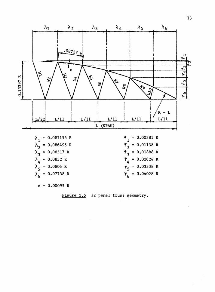
2.3, 2.4 and 2.5. All dimensions are to the center line of the mem
bers.
2.2.2 Details
10
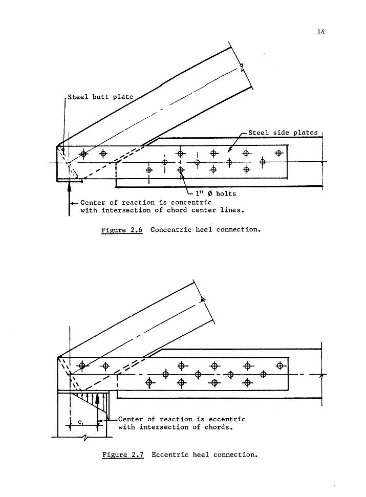
Figure 2.6 shows one type of heel connection being used. An
other similar type, shown in Fig. 2.7 has been commonly used. This
heel has the problem of inducing partial fixity into the bottom chord
as a result of the eccentric bearing. The effect of eccentric bearing
is studied in Chapter VIII.
Figure 2.8 shows a typical "strap and pin" web connection com
monly used. As can be seen, some joint slip in this connection would
be unavoidable. Fortunately, this will actually help relieve some of
the secondary moments by allowing the deflected shape to change to a
smoother curve.
Figure 2.9 shows a typical center line splice detail. Very
little curvature is found to exist at the center of the truss when de
flected. As a result, fixity or lack of fixity induced by the large
side plates is found to have negligible effect on the bending moments.
in the bottom chord.

A 1 ~ 2 ~3 " 4
~.~.i~.-~L-'7~~-~L~_L1_1 _____ ~~~i. ___ L_n ___ j~I c
0 L (SPAN) _
~ l = 0.130525 R
,.\ 2
= 0.128295 R
A 3 = 0. 123 86 5 R
).. 4
= 0.117315 R
e = 0.00214 R
'f' l = 0.00856 R
'/> 2
= 0.02551 R
'f 3
= 0.04205 R
'f 4
= 0.05785 R
Figure 2.3 8 panel truss geometry.
11
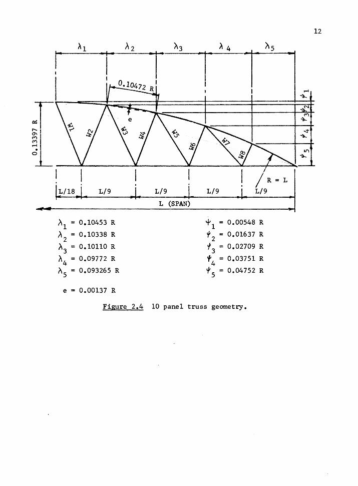
r ~l
,~ ~l
• I •
I ' I I
'
L/9
~l = 0.10453 R
~ = 0.10338 R 2
>.3
= 0.10110 R
~ 4 = 0.09772 R
~ 5 = 0.093265 R
e = 0.00137 R
Azl ~3
. • 1. L/9
L (SPAN)
~ 4
I T I
IR= L L/9 L/9
+ l = 0.00548 R
t2
= 0.01637 R
t/ 3 = 0.02709 R
t4
= 0.03751 R
'/'5
= 0.04752 R
Figure 2.4 10 panel truss geometry.
12
1'""'4 ~
N
('I")
~
..::t' ~
IJ"I ~
/\1 ~2
L/22 L/11
>.1
= 0.087155 R
~ 2 = 0.086495 R
).3
= 0.08517 R
~4 = 0.0832 R
~S = 0.0806 R
~ 6 = 0.07738 R
e = 0.00095 R
t\3
· 1
>.4
L/11 L/11
L (SPAN)
T Its
T /\6
L/11
! ;: = L
L/11
'/' l = 0.00381 R
'/' 2
= 0.01138 R
t3
= 0.01888 R
'f'4
= 0.02624 R
t5
= 0.03338 R
'f 6 = 0.04028 R
Figure 2.5 12 panel truss geometry.
13
I ..... ~
I ~
l" '/J bolts Center of reaction is concentric with intersection of chord center lines.
Steel side plates
Figure 2.6 Concentric heel connection •
..... .P.--Center of reaction is eccentric with intersection of chords.
Figure 2.7 Eccentric heel connection.
14

Single bolt. Shear plates each side if required for load.
2-3/4" bolts @ webs
strap each
\
Figure 2.8 Typical web connection.
steel side plates
l" </J bolts
Figure 2.9 Typical bottom chord splice.
15

CHAPTER III
COMPUTER MODELS
3.1 GENERAL INFORMATION
Computer models were developed for the three configurations
shown in Figure 2.1. These will be referred to as 8 panel, 10 panel
and 12 panel trusses in respect to the number of top chord sections or
"panels" they contain.
A basic 100 ft. span truss with the radius of the top chord
equal to the span was used for each configuration. In order to model
the curved top chord, each top chord panel was divided into four equal
straight segments. All loads were applied at the nodes.
The bottom chord panels were divided into two segments in order
to allow evaluation of tertiary (P-~) moments.
3. 2 EIGHT PANEL TRUSS
The eight panel truss was modeled in three different ways, using
two computer programs.
3.2.l Model I
A truss and frame analysis program entitled "RIGID"(3) was util
ized for this model. One half of the truss was modeled, with vertical
roller supports provided at the truss center line. A horizontal roller
support was used to model the column bearing support at the end of the

17
truss. The model is shown in Fig. 3.1.
The chords are modeled with beam elements to reflect the contin-
uous nature of the chords. A double roller support with a rigid truss
link between them was used at the heel to artificially provide the
member end releases. As can be seen from Fig. 2.6, the top chord is
essentially free to rotate in the connection. An internal hinge would
therefore seem appropriate. This technique provided the ability to
model heel joint slippage and joint fixity.
The peak connection was also modeled as a pinned joint. The
top chord of these trusses is normally spliced at the peak to facili-
tate fabrication and shipping. The connection is normally not substan-
tial enough to be considered capable of transferring moment.
All webs are modeled as truss elements i.e., no bending capacity
(I=O). Therefore, all web to chord connections are in essence pinned,
which is obviously the case in the real truss. (See Fig. 2.8.)
3.2.2 Model II
The second model considered was very similar to the first model,
except that it was developed using "SAP IV"(4) finite element program.
The same half truss was modeled with similar supports. This was used
as an independent check on the input/output information that was
gathered from the first model. Fig. 3.2 shows the model which was used.
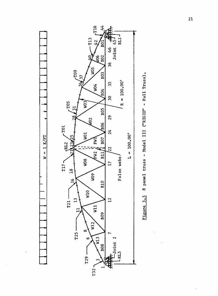
3.2.3 Model III
This model, using the program "RIGID", modeled the entire truss.
The purpose for this model was to observe unbalanced conditions, which
was not possible with the half truss of the first model. The diffi-

....
r-r-
1 r-
i-i-
rnrl
W
=lK
/FT
,
t l
l l
l-l-
ul'
l
'\Om
Uni
form
lo
ad a
pp
lied
to
tru
ss
as
con
cen
trat
ed
load
s at
each
no
de •
2 3
4 T04
B07
24
B
04
1.8
75
00
° so.o
o•
Str
aig
ht
segm
ents
b
etw
een
nod
es
B03
0
Rad
ius
=
Spa
n =
1
00
.00
'
Fig
ure
3
.1
8 p
anel
-
Mod
el
I ("
RIG
ID")
.
B02
I-'
00

L-f~
_-_L
] ___ L
l ___ _r
-rr--r
__ r
' w
= 1
K/F
T
, •
, 1
1 t
r-! -r
c~o
~Uni
form
load
ap
pli
ed t
o t
russ
as
co
nce
ntr
ated
lo
ads
at
each
no
de.
join
t 3
4
6 5
4 3
2
24
22
20
Rad
ius
=
Spa
n =
1
00
.00
'
50
.00
' T
op
and
bo
tto
m c
ho
rds
use
bea
m e
lem
ents
. W
ebs
use
tr
uss
el
emen
ts.
Str
aig
ht
segm
ents
be
twee
n no
des 1
Fig
ure
3.2
8
pan
el
-M
odel
II
(S
AP
IV)
23
18
Pin
ned
~
\0

20
culty encountered here was created by the fact that the current version
of the program does not provide for member end releases. Therefore,
modeling the internal hinge at the center of the top chord proved cum•
bersome. The member release was obtained by installing a short rigid
link at the center. In order to transfer shear across the joint, two
artificial web members were included in the model, as shown in Fig.
3.3.
This provided reasonable results when using the actual web areas
(no joint slippage). When providing for joint slip, however, the arti
ficial webs disrupted the deflections of the truss substantially. This
data is therefore not considered valid.
3.2.4 Loading
The loading assumed a one kip per foot uniform load on the top
chord, under fully balanced conditions. This load was converted to
concentrated loads to be applied to the truss at the node points.
The bottom chord of the truss was assumed to have no external
loading.
3.2.5 Variations
Several variations were made using Model I, to briefly study the
effects of several potential physical variations from the "ideal" model.
Effects of joint slippage, heel and bottom chord splice fixity were
considered.
3.2.5.1 Web Connection Bolt Slippage. As mentioned previously,
the type of connection shown in Figure 2.8 will be subject to joint
slippage, both at the pin bolt and also in the double bolt connection
LI
' . l
l r '
' l.
I . 1-
--,-
-r~ -~
----
;-~~
;;T
I t
t l
l ' n
--, H 1
r-n
T2
5--
T32
BlO
2 F
als
e w
ebs L
= 1
00
.00
'
Fig
ure
3
.3
8 p
an
el
tru
ss
-M
odel
III
("R
IGID
" -
Fu
ll T
russ
).
N
I-'

22
to the web itself. This effect was modeled by "softening" the web (re
ducing the area) to provide an additional 1/16 in. to 1/8 in. member
shortening or elongation. No attempt was made to establish an exact,
uniform amount of slip in all joints. The required area was back cal
culated from the member loads obtained from the first series of runs
using actual member areas. The resulting elongation did not exactly
yield the slip assumed due to redistribution of forces changing the
member forces. Further refinement seems unjustified in light of the
highly unpredictable nature of the slippage. Member misfit during fab
rication, hole size and straightness, temperature, moisture content and
residual stresses in the chords during fabrication will all affect the
amount of slip actually occurring in the real structure. This general
influence and its potential magnitude is what is of importance.
3.2.5.2 Heel Joint Slippage. The effect of joint slippage in
the heel connection was modeled by "softening" the rigid link connect
ing the two support rollers at the heel location.
3.2.S.3 Heel Joint Fixity. Some heel designs have the poten
tial of inducing full or partial fixity into the bottom chord at the
heel connection. This was modeled by fully fixing the roller connect
ing the bottom chord member. This therefore would simulate the worst
condition, providing an upper bound to examine the effect of fixity in
the heel.
3.2.S.4 Bottom Chord Splice Bolt Slippage. Joint slippage in
the center splice joint was modeled by specifying a specific horizontal
support displacement (.006 ft.) at the vertical roller at the bottom
chord.

23
3.2.5.S Bottom Chord Splice Fixity. The normal model assumes
the bottom chord to be pinned at the center. The effect of fixity
which may well be the case in the real truss was modeled by providing
rotational fixity to the roller joint.
3.2.S.6 Heel Plate Fixity, Chord Rotation Permitted at Bolts.
The possible, but unlikely, occurrance of the heel assembly being fixed
on the column, while the chord rotates at the bolted connection was
considered. The physical condition is shown in Fig. 3.4. This was
modeled by extending the length of the "rigid" link from .001 ft. to
2.5 ft. The area of the link was then reduced to simulate joint slip
in addition to the rotation.
3.2.S.7 Combinations of Effects. Web slippage combined with
heel slippage plus fixity was examined by combining the techniques used
above. Similar combinations were used for the center splice.
3.2.6 Member Properties
The chords of the truss were taken as Douglas Fir/Larch combin
ation no. 3 as defined under the AITC 117-79 Specifications. (S)
The design values given are shown in Table 3.1.

free to rotate about centroid of bolts
---7-? .... , -_-"' ___ -~--:......~ ~_, ~ $-
e
l 2.5' ..
Heel assembly f xed against rotatio due to eccentric be ring
2.5'
Figure 3.4a Physical condition.
. L , Figure 3.4b Computer model.
Figure 3.4 Fixed heel with rotation of bottom chord at bolts.
24

TABLE 3.1
DESIGN VALUES FOR STRUCTURAL GLUED LAMINATED TIMBER
COMBINATION NO. 3 AITC 117-79
Species DFL
Grade L2D
E l.8(106)psi
Ft 1450 psi
Fe 2300 psi
Fb 2000 psi xx
25
Combination no. 3 is connnonly used in trusses built in the Pac-
ific Northwest because it combines several desirable properties. Doug-
las Fir/Larch is the most readily available high strength material in
this region. Of the DFL combinations, only combination no. 5 has high-
er design values for tension, compression and bending. The advantage
of combination no. 3 is that in addition to high strength, L2D lamina-
ting stock (which is used in this grade) is a dense grained material
which permits the use of higher allowable connector loads. L2D stock
can be extracted from commonly supplied L2 stock, since a considerable
amount of the L2 stock meets the dense grade requirement.
The web members were assumed to have an E value of 1.6 (106)
psi.
The chord member areas and moments of inertia (I values) were
the principal parameters varied in developing the data. The areas and
I values were varied independently in order to produce correlations
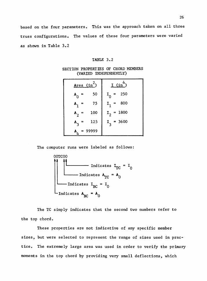
26
based on the four parameters. This was the approach taken on all three
truss configurations. The values of these four parameters were varied
as shown in Table 3.2
TABLE 3.2
SECTION PROPERTIBS OF CHORD MEMBERS (VARIED INDEPENDENTLY)
Area (in2) I (in4)
AO = 50 IO = 250
Al = 75 Il = 800
A2 = 100 12 = 1800
A3 = 125 I = 3600 3
A4 = 99999
The computer runs were labeled as follows:
OOTCOO
ft_ Indicates I.re = I0
L_____Indicates A.re = A0
Indicates IBC = 10
Indicates ~c = A0
The TC simply indicates that the second two numbers refer to
the top chord.
These properties are not indicative of any specific member
sizes, but were selected to represent the range of sizes used in prac-
tice. The extremely large area was used in order to verify the primary
moments in the top chord by providing very small deflections, which

27
results in very small secondary moments.
3.3 TEN PANEL TRUSS
The 10 panel truss was modeled as a half truss similar to the
8 panel Model I, using the RIGID program. See Fig. 3.5 for the model
description.
The same member properties and parameter variations were made
for the 10 panel as for the 8 panel Model I.
3.4 TWELVE PANEL TRUSS
A half truss was modeled using RIGID, similar to the 8 panel
Model I. See Fig. 3.6 for the model description. The same member
properties were used as for the 8 panel Model I. Heel and splice slip
and fixity were not considered in this model.

1 '
1 1
1 i H
-r-1---
r-T u r
-.-
w =
1 K
/FT
,
• *
1 i
i----i
i -1
-o~
tUn
ifo
rm l
oad
ap
pli
ed
to
tr
uss
as
con
cen
trat
ed
load
s at
each
no
de.
1
2 3
4
B09
BO
B
30
29
2
B06
BO
S B
04
26
25
50
.00
'
Rad
ius
=
Spa
n =
1
00
.00
'
Str
aig
ht
segm
ents
be
twee
n no
des
B03
24
23
Fig
ure
3.5
_ 10
p
anel
-
Mod
el
I ("
RIG
ID")
22
rrrr
rTJ
_j N
CX
>
I l
I l
l l
1 I
I I
I I
w ~ =
1 K
/FT
,
t '
l l
l I
i T IIL
J
\9 Un
ifo
rm l
oad
ap
pli
ed to
tr
uss
as
co
nce
ntr
ated
lo
ads
at
each
no
de.
2 3
4
B0
9
8
0 1
.25
B06
BO
S
20
Str
aig
ht
seg
men
ts
bet
wee
n n
odes
so.o
o•
Rad
ius
= S
pan
= 1
00
.00
' ~
Fig
ure
3.6
12
pan
el
-M
odel
I ~'RIGID").
N
\0

CHAPTER IV
PRIMARY MOMENTS IN THE TOP CHORD
4.1 METHODS OF ANALYSIS
In order to assess the secondary moments in the top chord, we
must first determine the primary moments which exist as part of the
moments computed by the computer analysis.
4.1.1 AITC Method
The existing design methodology as outlined in the AITC Timber
Construction Manual(2) uses the method of superposition when computing
the top chord bending moments. The moments for a continuous, straight
beam are added algebraically to the ''Pe" moments, assuming that the
''Pe" moments are distributed in the same manner as the uniform load
moments. The "Pe'' moment is the moment induced by the axial force, P,
in the chord acting through the eccentricity, e, of the curved member.
Secondary moments (i.e., those caused by joint displacement) are ne-
glected.
For example, for an 8 panel truss, the beam moment at the first
panel point would be computed as
M_ - - • 1071w i\ 2 -~eam -
which is 85.68% of the simple span moment (.8568xl/8w A 2). The .1071
factor is the moment coefficient for a four span continuous beam with
uniform load on all spans.

31
Thus,
M = .8568 [w8~2J - .8568 Pe
2 = .107lw ~ - .8568 Pe
This method is expected to give reasonably accurate results,
however a more accurate analysis is necessary here in order to accu-
rately separate the primary from the secondary moments (i.e., from
joint deflection induced moments).
The following method has been used for this purpose, and is pro-
posed for general use.
4.1.2 Moment Distribution
The moment distribution method requires that "fixed end" moments
be determined for each "span" of the continuous curved chord. These
"fixed end" moments (FEM) will consist of the moments induced by the
external loads applied to the member acting as a continuous beam, plus
the moments induced by the "Pe" effect. The equations for these FEM's
are as follows. The derivation of the equations is provided in Appendix
1.
4.1.2.l FEM due to "Pe". Referring to Figure 4.1,
(4.1)
4.1.2.2 FEM due to External Member Loads. The FEM due to the
loads on the member can be calculated assuming the beam to be a straight
beam with its length equal to the projected distance between the two
end points, A and B1 measured perpendicular to the axis of the load.
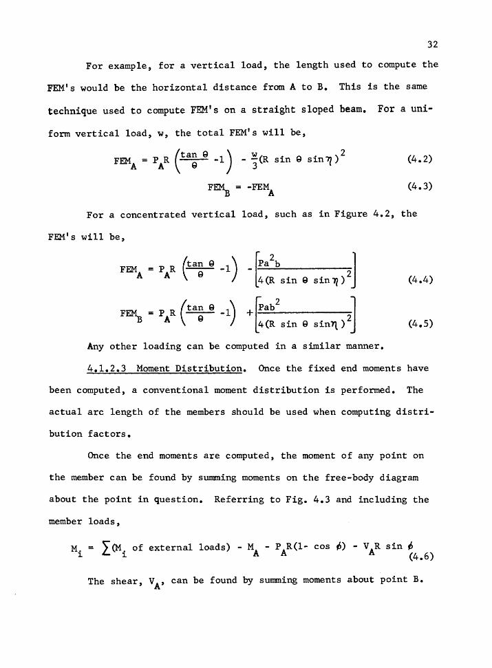
32
For example, for a vertical load, the length used to compute the
FEM's would be the horizontal distance from A to B. This is the same
technique used to compute FEM's on a straight sloped beam. For a uni-
form vertical load, w, the total FEM's will be,
FEMA = PAR (ta~ 9 -1) - ~(R sin Q sin71)
2
FEMB = -FEMA
(4. 2)
(4.3)
For a concentrated vertical load, such as in Figure 4.2, the
FEM' s will be,
FEM = p R (tan Q A A Q -1) ra2b
4(R sin Q sin 1/) iJ (4.4)
Ffil\ = p AR (ta~ Q -1) ~ 2 sin71.) i] + Pab
4(R sin Q (4.5)
Any other loading can be computed in a similar manner.
4.1.2.3 Moment Distribution. Once the fixed end moments have
been computed, a conventional moment distribution is performed. The
actual arc length of the members should be used when computing distri-
bution factors.
Once the end moments are computed, the moment of any point on
the member can be found by summing moments on the free-body diagram
about the point in question. Referring to Fig. 4.3 and including the
member loads,
M. = L (M1. of external loads) - MA - P AR(l- cos ;,) - VAR sin ;,
l. (4.6)
The shear, VA' can be found by summing moments about point B.

33
Figure 4.1 Fixed end forces on a top chord panel due to 'P x e'.
p
a b
Figure 4.2 Fixed end forces on a top chord panel due to a concentrated load.

k--.eMA _r- R sin fl i G/"~ L~ R(l-cos 0)
0
VA·~
P. ].
Figure 4.3 Free-body forces on a top chord segment.
34

35
Thus,
l~ external loads) - MA - ~ - PAR{l - cos 2Q)
R sin 2Q (4. 7)
The procedure is demonstrated on the following pages where the
primary moments in the 8, 10 and 12 panel trusses subjected to a uni-
form vertical load are computed.
Figure 4.4 provides the loading and geometrical data required
for determining the primary moments in the top chord of an 8 panel
truss. The axial forces listed in the figure are those in the chords
as obtained from a pin jointed analysis assuming straight line seg-
ments between panel points.
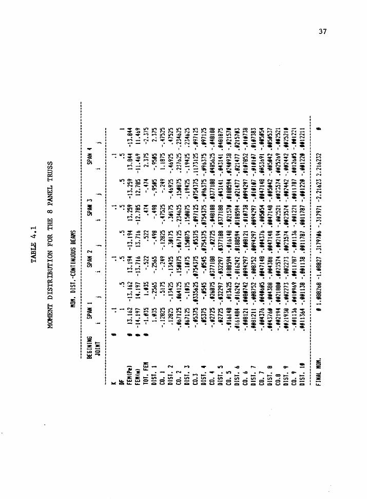
Table 4.1 shows the moment distribution calculations for the
top chord of the 8 panel truss. The fixed end moments listed are com-
puted from Equations 4.2 and 4.3. For clarity, the fixed end moments
due to "Pe" and due to the external loads are calculated and listed
separately.
The moment at intermediate points along the top chord of the 8
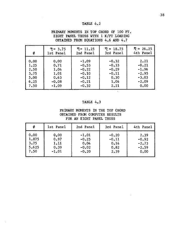
panel truss were computed using Equations 4.6 and 4.7. These values
are listed in Table 4.2, and plotte~ by a solid line in Fig. 4.5.
Data obtained from a computer frame analysis (Model I) in which very
large member areas were used is plotted as a dashed line in Fig. 4.5.
As discussed in Chapter III, the use of large member areas nearly elim-
inates the secondary moments induced from the deflection of the truss
joints. Some slight deflection still occurs, owing to both the axial
deformation of the members and to the moments acting on the curved top

36
chord. Therefore some small amount of secondary moment will exist in
the computer data. As will be seen in later chapters, the secondary
moments are positive along the entire length of the top chord. From
this, it would be expected that the moments obtained from the computer
analysis would be slightly greater (more positive) than the actual pri-
mary moment.
As can be seen from Fig. 4.5, the computer produced moments do
plot slightly higher than, but very close to the moments computed using
the method proposed in this chapter.
Figure 4.6 together with Tables 4.4 and 4.5 provide the data
required to produce the primary moment diagram for the 10 panel truss
which is plotted in Fig. 4.7. This data is computed in the same manner
as for the 8 panel truss.
The procedure is repeated for the 12 panel truss. Fig. 4.8 and
Tables 4.6 and 4.7 provide the necessary data. The diagram for the
primary moment in the top chord of the 12 panel truss is plotted in
Fig. 4.9.
The data produced in this chapter will be used in Chapter VI to
separate the primary moment out of the total moments in the top chord
obtained from the computer analyses. This will be done in order to
study the magnitude of the secondary (joint movement induced) moments.
K DF
FE"<
Pe)
FUt•>
TO
T. FE
M DI
ST.
1 co
. 1
DIST
. 2
co.
2 DI
ST.
3 C0
.3
DIST
. 4
co.
4 DI
ST.
5 co
. s
DIST
. 6
co.
6 DI
ST.
7 co
. 7
DIST
. B
co
.a DI
ST.
9 co
. 9
DIST
. lt
BEGI
N IN
G JO
INT
FINAL
"O"
.
TABL
E 4
.1
MOM
ENT
DIS
TRIB
trrIO
N F
OR T
HE
8 PA
NEL
TRUS
S
"O".
DIST
.-CON
TINU
OUS
BEA"
S
SPAN
l
SPAN
2
SPAN
l
SPAN
4
• . l
• 1
• l
.1
1
.s .5
.5
.s
.5
.s l
• 13
.162
-1
3.16
2 ll.
194
-13.
194
13.2
59
-ll.2
S9
ll.84
4 -1
3.84
4 •
-14.
197
14. J
CH
-13.
716
13.7
16
-12.
785
12.7
85
-11.
469
l l .4
69
• -1
. 835
1.
135
-.522
.5
22
.474
-.4
74
2.:m
-2
.375
1.
835
-.256
5 -.2
565
-.498
-.4
98
-.958
5 -.9
585
2.37
5 -.1
2825
.5
175
-.249
-.1
2825
-.4
7525
-.2
49
l.187
5 -.4
7515
.1
2825
-.1
3425
-.1
3425
.3
1175
.3
•175
-.4
6925
-.4
6925
.U
525
-.t6
7t25
.8
641~
5 .1
5t87
5 -.t
6112
s -.2
3462
5 .1
~101
5 .2
37b2
S -.2
34a2
5 .1
6712
5 -.1
175
-.lt
JS
.151
875
.158
875
-.194
25
-.194
25
.234
625
-.853
75 .
1335
625
.t754
375
-.153
75 -
.t971
25 .
8754
175
.117
3125
-.1
9712
5 .8
5375
-.1
545
-.854
5 .1
7543
75 .
8754
375
-.896
375
-.896
375
.t971
25
-.f27
25
.826
875
.837
7188
-.8
2725
-.1
4818
8 .tl
7718
8 .8
4856
25 -
.148
188
.827
25 -
.132
297
-.832
297
.137
7188
.83
7718
8 -.
t4ll
41 -
.841
141
.848
1875
-.1
1614
8 .8
1362
5 .1
1885
94 -
.tl6
l48
-.121
578
.tt88
594
.t24t
93B
-.1
2157
8 .1
1614
84 -
.816
242
-.816
242
.118
8594
.81
8859
4 -.t
2147
7 -.1
2147
7 .8
2157
13
-.908
121
.188
1742
.18
9429
7 -.t
t812
1 -.t
1173
8 .1
1942
97 .
1117
852
-.tl
t738
.~
8812
11
-.888
752
-.888
752
.189
4297
.88
9429
7 -.
tltl
t7 -
.tlt
li7
.tlt
7383
-.t
8437
6 .1
8416
85 .
tt471
4B -
.tl4
l7o
-.t85
854
.tl47
14B
.te
53b9
l -.8
1585
4 .8
t437
6t -
.884
388
-.814
388
.884
7148
.11
4714
8 -.8
1584
2 -.f
t514
2 .lt
5t53
7 -.9
02!9
4 .tl
2188
8 .8
8235
74 -
.tt21
94 -
.182
521
·'•2
~574
.fi
252b
9 -.1
1252
1 .1
1219
38 -
.882
273
-.882
273
.111
3574
.88
2357
4 -.
tt144
2 -.1
8244
2 .8
t252
11
··.H
l1l6
.t•
ll'ib
9 .H
l178
7 -.
ttll
l6 -
.H12
1l .
ftl1
787
.111
2615
-.H
l22l
.•
tt136
4 -.1
8113
8 -.
8111
~8
.ttl
l787
.11
1178
7 -.1
8122
1 -.8
1122
8 .1
1122
11
t t.8
8826
8 -1
.888
27 .
3179
786
-.317
971
-2.2
1623
2.2
1623
2 8
w
......
"' o.oo 1.25 2.50 3.75 5.00 6.25 7.50
"' o.oo 1.875 3.75 5.625 7.50
TABLE 4.2
PRJMARY MOMENTS IN TOP CHORD OF 100 FT. EIGHT PANEL TRUSS WITH 1 K/FT LOADING
OBTAINED FROM EQUATIONS 4.6 AND 4.7
7l= 3.75 11 = 11. 25 11.= 18.75 1st Panel 2nd Panel 3rd Panel
o.oo -1.09 -0.32 0.71 -0.53 -0.33 1.04 -0.22 -0.29 1.01 -0.10 -0.11 o.63 -0.12 0.30
-0.08 -0.21 1.04 -1.09 -0.32 2.21
TABLE 4.3
PRlMAR.Y MOMENTS IN THE TOP CHORD OBTAINED FRCM COMP'UTER RESULTS
FOR AN EIGHT PANEL TRUSS
1st Panel 2nd Panel 3rd Panel
o.oo -1.01 -0.20 0.97 -0.25 -0. ll 1.ll 0.04 0.14 0.39 -0.02 0.82
-1.01 -0.20 2.39
38
'2 = 26. 25 4th Panel
2.21 -0.21 -1.96 -2.95 -3.03 -2.09 o.oo
4th Panel
2.39 -0.92 -2.73 -2.59 o.oo

~
' ~ µ..
~
~ ~
~ •r-1 ~
Pot ........ u ~
{ 1 l l l ' l I 'w = 1 K/FT l I ' t 1 l I l J 1
50.00'
11 -= 3.75° A = 13.0525' PAl = 92.02 K 1 1
1l 2 = 11.25° A = 12.8295' PA2 = 92.24 K 2
113 = 18.75° ~3 = 12.3065' PA3 = 92.70 K
7l = 26.25° ~4 = 11.7315' PA4 = 96.79 K 4
Figure 4.4 8 panel truss - primary moment data.
3.0
2.0
1.0
Computer
0
-1.0
-2.0
-3.0·
~ Truss Heel
Figure 4.5 Primary moment diagram for a 100 ft. span 8 panel truss - one kip per ft.
39

K DF
Fn<P
e)
FEn(
•t TO
T. FE
ft DI
ST.
1 co
. l
DIST
. 2
co.
2 DI
ST.
l C0
.3 DI
ST.
4 co
. 4
DIST
. 5
co.
5 DI
ST.
6 co
. 6
DIST
. 1
co.
1 DI
ST.
8 co
.a DI
ST.
9 co
. 9
DIST
. 11
BEGI
NlNG
JO
INT
TAB
LE 4
.4
MOM
ENT
DIS
TR
IBU
TIO
N F
OR
TH
E 1
0 P
AN
EL
TRU
SS
"O".
DlST
.-CON
TINU
OUS
BEA"
S
SPAN
I
SPAN
2
SPAN
3
SPAN
4
SPAN
5
I .I
.I
.1
.l
.l
l
.5
.5
.5
.s .5
.5
.5
.5
l
I 8.
596
-8.5
96
8.59
9 -8
.599
8.
62
-8.6
2 8.
595
-B.5
95
8.93
2b7
-8.9
3207
I
-9.1
1533
9.
1153
3 -8
.987
8.
9t7
-8.5
19
8.51
9 -7
.958
7.Y
58 -
7.24
867
7.24
86b7
I
-.519
33
.599
33
-.318
.3
88
.ltl
-.
ltl
.637
-.6
37 l
.b84
~j3
-1.b
84
.589
33 -
.18t
obS
-.lt
t6b5
-.2
145
-.2t4
5 -.2
68
-.2bB
-.5
2351
2 -.5
2351
2 l.b
84
-.158
333
.254
665
-.112
25 -
.15t
333
-.134
-.1
1225
-.2
b175
l -.1
34
.842
-.2
6175
1 .t5
tl325
-.1
7628
8 -.1
7628
8 .8
9216
63 .
t92l
66l
.l82
ttt4
.18
2119
4 -.3
54
-.l5
4 .2
6l75
f8
-.138
184
.125
1663
.14
6183
1 -.1
381i
4 .1
9188
12 .
8461
831
-.177
.89
1818
2 .1
3187
54
-.177
.1
3811
38 -
.835
625
-.135
625
-.126
448
-.t2b
448
.t654
584
.165
4584
-.1
1193
8 -.1
1893
8 .1
77
-.117
812
.119
8519
-.8
1322
4 -.8
1781
2 .1
3272
92 -
.113
224
-.IS5
4b9
.132
7292
.i8
85 -
.t554
b9
.tl78
123
-.882
914
-.812
914
-.tt7
458
-.187
458
.834
3465
.83
4346
5 -.t
6t61
5 -.•
6161
5 .1
5546
89
-.tt1
457
.118
9162
-.8
8372
9 -.8
8145
7 .8
1717
33 -
.tt37
29 -
.831
387
.117
1733
.12
7734
5 -.
tJt3
f7
.111
4569
-.8
8258
8 -.8
1258
8 -.t
t785
8 -.1
1785
8 .1
1711
83 .
1171
183
-.122
454
-.122
454
.t3t3
t73
-.111
294
.188
7285
-.1
8392
9 -.8
1129
4 .1
1851
91 -
.113
929
-.111
227
.118
5891
.1
1515
37 -
.111
227
.111
2942
.18
1618
3 .1
1168
83 -
.113
617
-.183
617
.tt75
7Bt
.117
5781
-.1
1183
1 -.
ttlB
ll .
lll22
b9
.ttt8
812
.188
6471
-.8
i18t
4 .1
888t
t2 .
8137
891
-.181
814
-.885
916
.8t3
789f
.tt5
6135
·.8
1591
6 -.
ttt8
11 .
1885
783
.888
5783
-.tt
2295
-.1
1229
5 .1
1385
97 .
1138
597
-.814
711
-.tl4
711
.185
9157
.1
1120
92 -
.e~j
4tt
-.es
tt47
.tt8
2892
.11
1929
9 -.
ttti
47
-.1
1235
1 .tt
t929
9 .1
8295
78 -
.112
3s1
-.188
289
.181
7737
.88
8773
7 -.
tlll
lt -
.181
111
.111
7491
.11
1749
1 -.8
1244
4 -.f
t244
4 .1
8235
tb
.lti3
Bb8
-.S
!l145
-.8
8855
5 .8
8838
68 .
1118
745
-.111
555
-.881
222
.818
8745
.t•
lt75
3 -.t
•122
2 -.1
8838
7 .1
8934
97 .
1883
497
-.118
631
-.188
bll
.188
8883
.18
1888
3 -.
t~lt
25 -
.ttl
t25
.11
1221
9 .8
1817
48 -
.~~i
l93
-.188
315
.ttl
l748
.18
1444
2 -.1
1831
5 ·,f
jl51
2 .1
1~44
42
.111
6111
-.i
it5l
2 -.1
1817
5 .1
1125
44 .
1112
544
-.111
318
-.181
311
.188
4139
.81
1411
9 -.
lti5
28 -
.ftt
528
.llt5
124
FINAL
no"
. I
.68~
3136
-.b
f331
4 .8
3861
19 -
.138
611
-.l~
b5SB
.1
3655
79 -
1.71
659
l.7tb
588
I .i;
:..
0
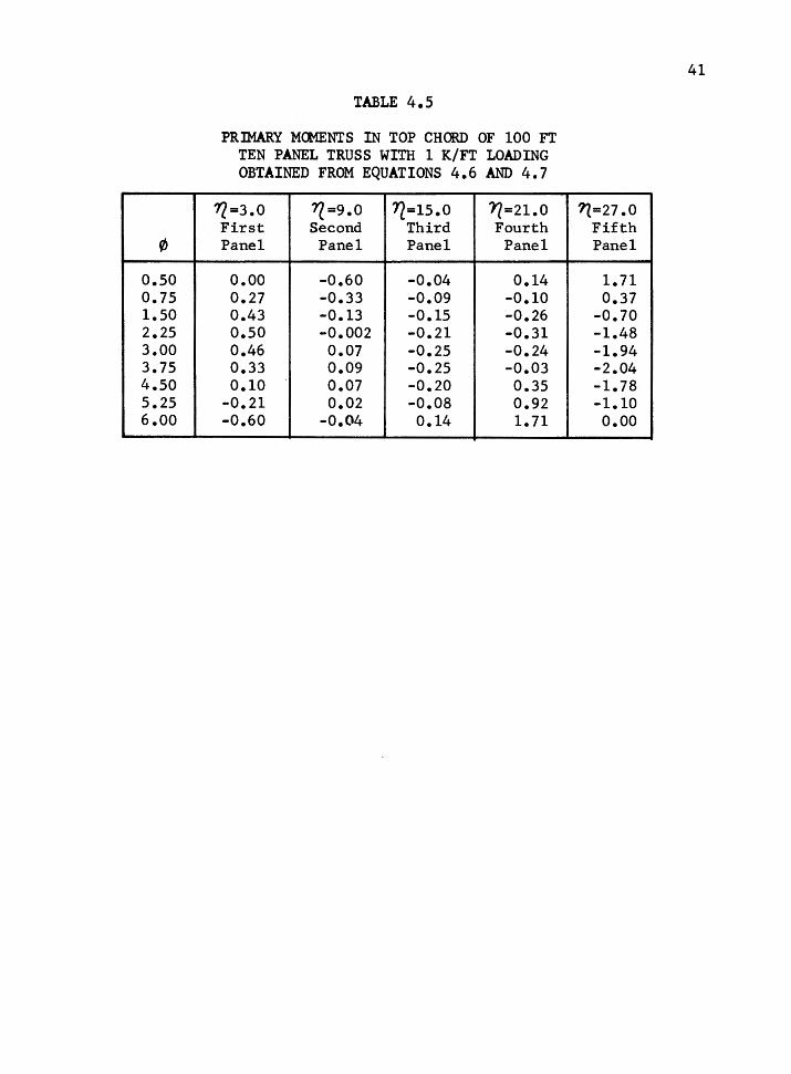
"' a.so 0.75 1.50 2.25 3.00 3.75 4.50 5.25 6.00
TABLE 4.5
PRlMARY MCMENTS IN TOP CHORD OF 100 FT TEN PANEL TRUSS WITH 1 K/FT LOADING OBTAINED FROM EQUATIONS 4.6 AND 4.7
7{=3.0 ?(=9.0 7l=l5.0 17=21.0 First Second Third Fourth Panel Panel Panel Panel
o.oo -0.60 -0.04 0.14 0.27 -0.33 -0.09 -0.10 0.43 -0.13 -0.15 -0.26 o.so -0.002 -0.21 -0.31 0.46 0.07 -0.25 -0.24 0.33 0.09 -0.25 -0.03 0.10 0.07 -0.20 0.35
-0.21 0.02 -0.08 0.92 -0.60 -0.04 0.14 1.71
41
11=27 .o Fifth Panel
1.71 0.37
-0.70 -1.48 -1.94 -2.04 -1.78 -1.10 o.oo
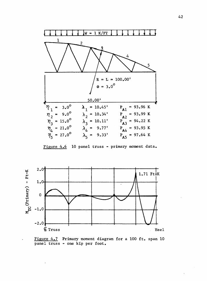
~ I
4.J µ...
,..... t( ctS e
•r-1 ,... P-4 '-'
c..:>
~
~ I l l l l I 1 w = 1 K/FT l 1 l 1 1 ' ' I I 1
9 = 3.0°
50.00'
12 1 = 3.0° ;.\ = 1
10.45' PAl = 93.96 K
Yl = 9.0° >. = 10.34' p = 93.99 K 2 2 A2
l? = 1s.0° ~ = 10.11' PA3 = 94.22 K 3 3
11 = 21.0° ~ = 9. 77' PA4 = 93.95 K 4 4
"ls = 27.0° A = 9.33' PAS = 97.64 K 5
Figure 4.6 10 panel truss - primary moment data.
2.0
1.
0
-1.0
-2.0
'f Truss
1.71 Ft K I
Heel
Figure 4.7 Primary moment diagram for a 100 ft. span 10 panel truss - one kip per foot.
42

K
DF
FE"<
Pe)
FE"h
t) TO
T. FE
" DI
ST.
l co
. 1
DIST
. 2
co.
2 DI
ST.
3 C0
.3 DI
ST.
4 co
. 4
DIST
. 5
co.
5 DI
ST.
6 co
. b
DIST
. 7
co.
7 DI
ST.
8 co
.a DI
ST.
9 co
. 9
DIST
. 11
BE61
NlN6
JO
INT
TABL
E 4
.6
MOM
ENT
DIS
TR
IBU
TIO
N F
OR
TH
E 1
2 P
AN
EL
TRU
SS
"°"· DI
ST.-C
ONTIN
UOUS
BEA
"S
SPAN
l
SPAN
2
SPAN
3
SPAN
4
SPAN
5
SPAN
b
j
t .l
.1
.l
.1
.l
.I
l
.5
.5
.5
.s .5
.5
.5
.5
.5
.5
l
t 5.
914
-5.9
14
5.89
5 -5
.895
5.
988
-5.9
t8
5.93
4 -5
.934
5.
b75
-5.6
75 5
.B95
33l
-5.6
9533
I
-6.3
3 6.
ll
-b.2
34
6.23
4 -6
.145
6.
145
-5.7
69
5.76
9 -S
.413
5.
413
-4.9
9 4.
9,
t -.4
16
.416
-.3
39
.3lq
-.1
37
.ll7
.1
65
-.165
.2
62
-.262
.9t
53l3
l -.9
1533
3 .4
16
-.838
5 -.8
385
-.111
-.1
11
-.151
-.1
51
-.t4
8j
-.S48
5 -.3
1166
7 -.3
2166
7 .Y
f533
3 -.
tt925
.2
ee
-.es
ss
-.119
25
-.875
5 -.
t5f5
-.1
2425
-.1
755
-.lot
BJ3
-.1
2425
.45
2006
5 -.
1ota
3l
.tl92
5 -.8
7875
-.1
7875
.1
4737
5 .8
4737
5 .1
3737
5 .8
3737
5 .1
1816
67 .
1181
b67
-.214
2t8
-.214
2•8
.168
8333
-.1
1937
5 .1
8962
5 .1
2368
75 -
.139
375
.118
6875
.t2
3687
5 .1
5988
33 .
1186
875
-.187
114
.159
1833
.tB
t416
7-.lt
7114
.1
3937
5 -.1
1665
6 -.8
1665
6 .1
1834
38 .
8113
438
-.141
385
-.841
385
.844
2183
.14
4288
3 -.1
6975
-.t
b975
.lt
?\t4
1 -.
tte1
2e .
1196
875
.1es
1119
-.tt
B32
8 -.1
2109
3 .1
1s11
19 .
1221
142
-.t2t
693
-.t34
B75
.t2
21t4
2 .8
5355
21 -
.t34e
7s
.118
3281
-.1
1243
8 -.8
1243
8 .1
1451
84 .
1145
114
-.t13
b38
-.113
638
.127
7839
.t2
7783
9 -.1
3782
8 -.8
3782
8 .1
34e7
S -.1
8621
5 .18
4164
1 .1
8725
52 -
.116
215
-.116
819
.117
2552
.11
3891
9 -.1
1681
9 -.1
1891
4 .1
1389
19 .
tl743
7S -
.flB
~l4
.tt62
148
-.885
711
-.185
7li
.186
5169
.11
6516
9 -.1
1157
4 -.8
1857
4 .1
1286
65 .
1128
665
-.tl5
b65
-.1!5
665
.118
9141
-.8
1285
5 .1
1311
74 .
8832
585
-.812
855
-.185
287
.113
2585
.11
6433
3 -.1
8528
7 -.8
8783
2 .tt
643l
3 .1
8945
78 -
.tt7B
32
.112
8548
-.8
8318
3 -.8
8318
3 .t
t4t7
t8 .
ft41
7t8
-.114
846
-.814
846
.116
5596
.ttb
5596
-.1
1794
5 -.1
1794
5 .tf
7832
4 -.1
1159
1 .1
1142
74 .
8821
354
-.111
591
-.812
423
.tt21
354
.113
2798
-.e
t242
3 -.1
1397
3 .1
8327
98 .
8139
162
-.tf
l97
l .1
1159
15 -
.881
731
-.881
731
.182
1172
.18
2817
2 -.1
8265
8 -.8
8265
8 .8
1319
78 .
8131
978
-.183
598
-.it
l598
.tt3
9726
-.
ttl8
66 .
1887
957
.80l
f836
-.8
1886
6 -.8
1132
9 .8
1111
36 .
ttl59
89 -
.111
329
-.tt
l799
.11
1598
9 .tl
l98b
3 -.
tt17
9'
.tt8B
657
-.tt
898t
-.e
0e9e
e .t
ttt9
72 .
8818
972
-.tt
l3tt
-.8
11J1
1 .1
1156
39 .
e115
o39
-.tt
t79l
-.e
e11q
3 .t
tt79
Yt
-.tt
t45
t .l
tt4l
29 .
t3i5
4B6
-.et
t45t
-.tt
tb51
.ttt
54B
6 .1
1110
19 -
.ttt6
51 -
.tttB
9b .
tt11e
19 .
ttt8
~95
-.tt
te9b
.tt
t449
8 -.t
,149
1 -.8
0949
1 .tt
8ss0
2 .1
1tss
e2 -
.ttt
665
-.t8t
665
.881
7735
.te
e11J
s -.
tet8
41 -
.~tt
e4t
... t
89bl
-.8
1824
5 .1
8822
49 .
tf827
5l -
.ttl
245
-.188
333
.188
2751
.1
8838
67 -
.tll
lll
-.888
428
.188
3867
.ttt
4481
-.f
fl42
1 .tl
t245
4 -.8
8125
1 -.8
8125
t .8
1828
91 .
8882
891
-.111
331
-.181
331
.111
3765
.11
1376
5 -.
ttl4
17 -
....
417
.tfl4
214
FINAL
"Oft.
I .5
t~S6
46 -.5
8486
5 .2
4550
54 -
.245
585
-.159
287
.159
2871
-.1
9234
9 .8
9234
95 -
.852
412
.852
4116
I
+:' w

0
o.oo 0.63 1.25 1.88 2.50 3.13 3.75 4.38 5.00
TABLE 4.7
PRlMARY MCMENTS IN TOP CHORD OF 100 FT. TWELVE PANEL TRUSS WITH 1 K/FT LOADING
OBTAINED FROM EQUATIONS 4.6 AND 4.7
1l =2.5 'T/. =7 .5 11=12.5 7l=l7.5' ?1=22.5 First Second Third Fourth Fifth Panel Panel Panel Panel Panel
o.oo -0.50 -0.25 0.06 0.09 0.21 -0.25 -0.12 -0.05 0.01 0.35 -0.06 -0.04 -0.15 -0.06 0.40 0.05 0.02 -0.23 -0.08 0.37 0.10 0.04 -0.28 -0.05 0.27 0.09 o.05 -0.28 0.04 0.08 0.02 0.05 -0.22 0.21
-0.17 -0.09 0.05 -0.11 0.48 -0.50 -0.25 0.06 0.09 0.85
44
~=27 .5 Sixth Panel
0.85 0.14
-0.43 -0.85 -1.09 -1.14 -0.99 -0.61 o.oo

~ I
,j.J
~
,.... t' ~
•r..f
"" Pot .......... u
~E-f
l l l ! l I l w = 1 K/FT J l 1 l l J 1 1 l
! R = Ji = 100.00' Q = 2.50°
.2Q.QQ'
11 = 2.5° A = 8.72' PAl = 93.12 K 1 l
'12 = 7.5° ,\ = 8.65' PA2 = 92.82 K 2
'l 3 = 12.5° ~ = 8.52' PA3
= 93.02 K 3 7l4 = 17.5° ~ = 8.32' PA4 = 93.44 K 4
115 = 22.5° ns = 8.06' PAS = 89.35 K
1l = 27.5° ~6 = 7.74' · P = 92 83 K 6 A6 •
Figure 4.8 12 panel truss - primary moment data.
2.0
1.
0
-2.
t Truss Heel
Figure 4.9 Primary moment diagram for a 100 ft. span 12 panel truss - one kip per foot.
45
CHAPTER V
SECONDARY MOMENTS IN THE BOTTOM CHORD
As defined earlier, the secondary moments are "support settle
ment" type moments induced into the continuous chord as the truss de
flects under load. In this case, the secondary moment in the bottom
chord will be equal to the total moment since we have assumed a
straight bottom chord with no direct loading on the bottom chord mem
bers.
5.1 PARAMETERS AFFECTING THE SECONDARY MOMENT IN THE BOTTOM CHORD
The principal parameters affecting the secondary moments in the
bottom chord are the values of the area and moment of inertia of both
the top and bottom chords, the load intensity, truss span and the num
ber of panels.
These parameters are designated as shown in Table 5.1. As indi
cated in Chapter III, the A and I values were varied independently over
a range of values encompassing the normal range of member sizes used in
practice. This range was listed in Table 3.2.
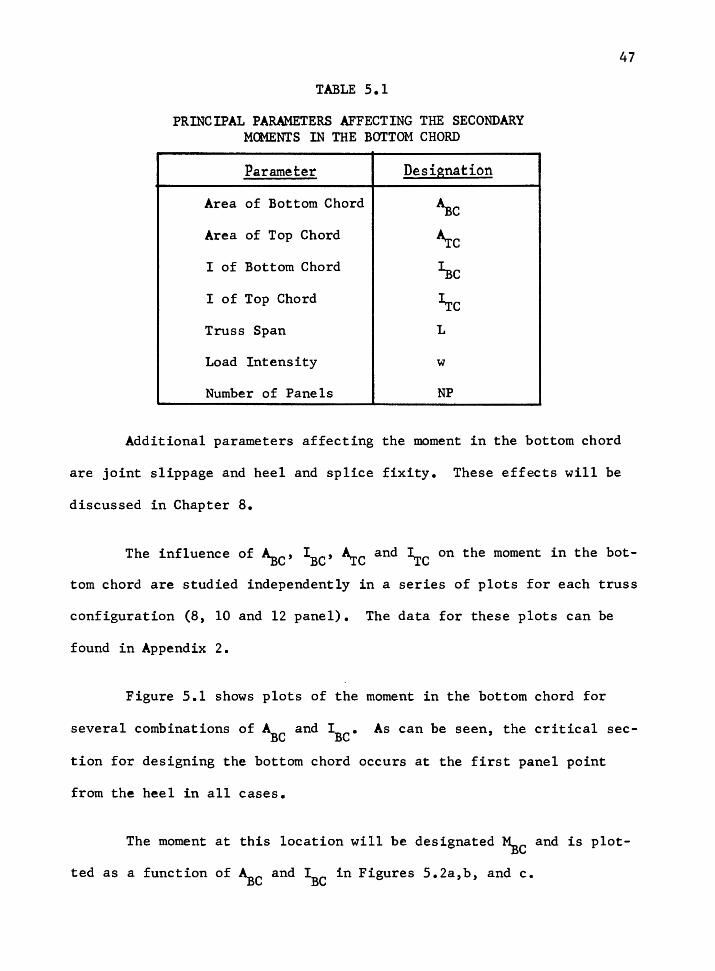
TABLE 5.1
PRINCIPAL PARAMETERS AFFECTING THE SECONDARY MOMENTS IN THE BOTTOM CHORD
Parameter
Area of Bottom Chord
Area of Top Chord
I of Bottom Chord
I of Top Chord
Truss Span
Load Intensity
Number of Panels
Designation
'\c
~c
~c
1tc L
w
NP
47
Additional parameters affecting the moment in the bottom chord
are joint slippage and heel and splice fixity. These effects will be
discussed in Chapter 8.
The influence of ~C' IBC' ~C and I.re on the moment in the bot
tom chord are studied independently in a series of plots for each truss
configuration (8, 10 and 12 panel). The data for these plots can be
found in Appendix 2.
Figure 5.1 shows plots of the moment in the bottom chord for
several combinations of ABC and !Be• As can be seen, the critical sec
tion for designing the bottom chord occurs at the first panel point
from the heel in all cases.
The moment at this location will be designated ~C and is plot
ted as a function of '\c and IBC in Figures 5.2a,b, and c.
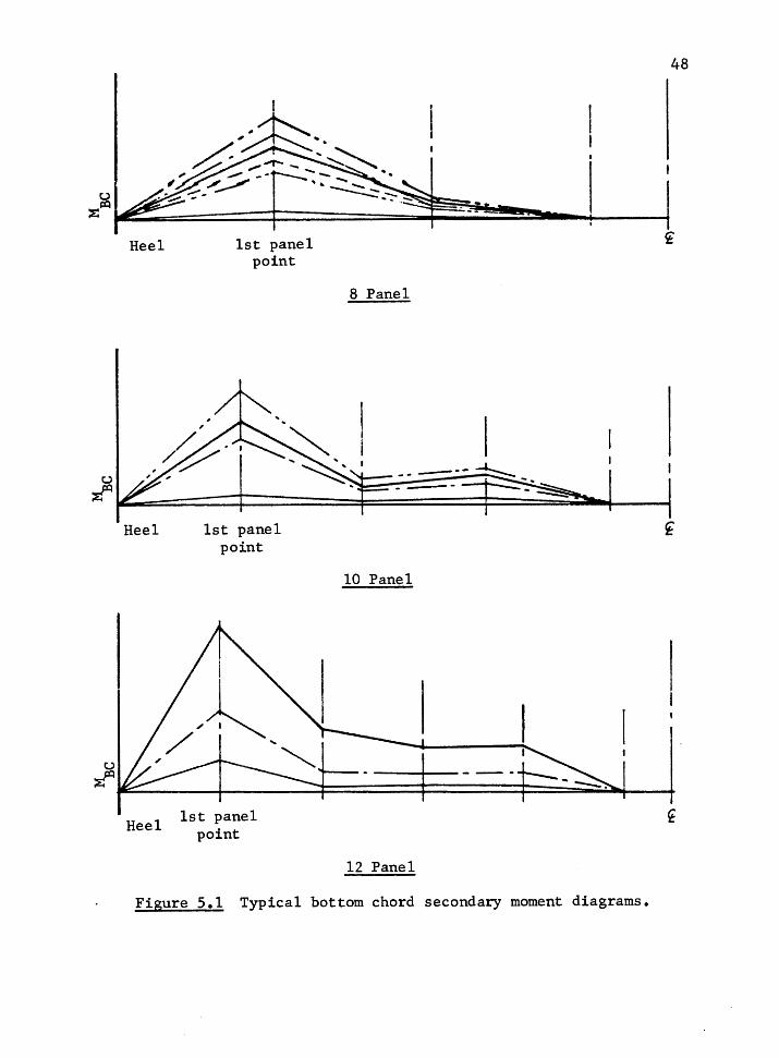
48
Heel 1st panel point
8 Panel
Heel 1st panel point
10 Panel
u
~~~~-+----~.::::;:===-=-=~~-==-=-~==-::t===~:.L---1.
Heel 1st panel
point
12 Panel
Figure 5.1 Typical bottom chord secondary moment diagrams.

24
22
20
18
16
14
12
,..... 10 ~
I +J ~ ........
t.) 8 ~
6
4
2
0
49
(!)=computer data
x = computed from Eq. 5 .11
\
+ \ I
\
A = 75.( ~ . 2 \ in G\ TC I in4
I = 800.( ... .Lv ""' L = 100.( , ft. ' ,;--I = 3600
w = i K/ t. ....... ·-= j T ................
.1-........ ...__ . --..cl ~
't
\
" ' ' '~ ~, / .... ~c = 1soo ......
~~ I ----
w ____ ... ---; .___
,, ' ' .......... ~
...___ --- _;_: "-1 = 800 BC
~ ..... "" .... -----i II-r -~c = 250 , ..... ~
--... --1 ~--1..., P.---~ t---~ r-
0 25 75 100 125
Figure S.2a 8 panel truss - secondary moment in the bottom chord as a function of ABC and IBc•

24
22
20
18
16
14
12
10 ,...... ~ I
+J ~ 8 ....,,
t,)
~ 6
4
2
0
50
G> = computer data
x = computed from Eq. 5.11
A.re = 75.! in2
)L. I I I
,,, -r-·
' I I I..r.~ = 800.~ in
4 ' ' I ... - '-f: 1iic = :$bUl
-t--L = 100.c I ft. I W= 1 K/j t. I I , --- ......... I
I I
"""'j ........... I
......__ __ ..._ ...._
I I () I I
\ I I I I I
\ I
I \ I 'I.. I
" I
'"') I ,,, I I
I ~ '~~c= 180I
I I "'"' ....... ____
I l ·~-- I
l I - -~""--,,,
I I ' I ...............
......._ ' .. -~----~_1ii_::_80l I
I - I -----.,r.-i l
~It--.-- --- / ._I = 250
BC i.r-----::Z..Jj ~---- 0
---~ ~
0 25 75 100 125
Figure S.2b 10 panel truss - secondary moment in the bottom chord as a function of ~C and !Be•
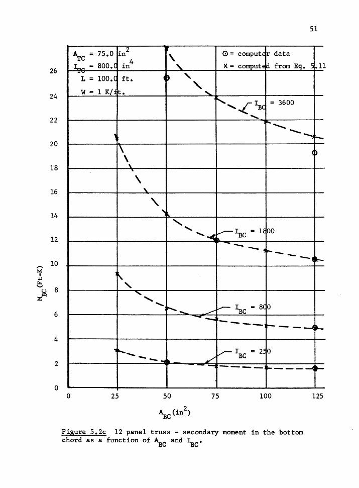
26
24
22
20
18
16
14
12
10 ,.... ~ I
+J ~
"'"' 8 u ~
6
4
2
0
51
\c= 75.0 . 2 r 0 = compute r data in \ . 4 L_ = 800.C in ' X = compute d from Eq. 5 .11
... 'W
' L = 100.C ft. 0
' w = 1 K/f !t. ' ·~ '~~( = 3600
' ·~ ............ , ..........._~ ~
\ ~~ \ ' '
\ '
' ~ ... ' ' ~~c=H 00
'...c£ "' - ---
-- i ..... __ -- --· ~ l'
' ' ' 'i ........... .........._ __.,.,.. ~ ~c = 8CO -- --.. ·- ---· ~ -- .... I ........
.,,...._, V- IBC = 2~ 0
"""-. ...... / -- .... ~ - _,,, --~-: "------4 .....
0 25 75 100 125
Figure 5.2c 12 panel truss - secondary moment in the bottom chord as a function of ~C and ~c·
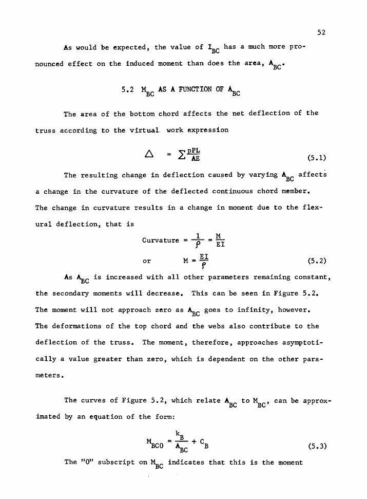
As would be expected, the value of 1:sc has a much more pro
nounced effect on the induced moment than does the area, ~c·
5. 2 MBC AS A FUNCTION OF ~C
52
The area of the bottom chord affects the net deflection of the
truss according to the virtual. work expression
(5.1)
The resulting change in deflection caused by varying ABC affects
a change in the curvature of the deflected continuous chord member.
The change in curvature results in a change in moment due to the flex-
ural deflection, that is
1 M Curvature = --p- = EI
EI M =-r or (5. 2)
As ~C is increased with all other parameters remaining constant,
the secondary moments will decrease. This can be seen in Figure 5.2.
The moment will not approach zero as ~C goes to infinity, however.
The deformations of the top chord and the webs also contribute to the
deflection of the truss. The moment, therefore, approaches asymptoti-
cally a value greater than zero, which is dependent on the other para-
meters.
The curves of Figure 5.2, which relate ABC to MBC' can be approx
imated by an equation of the form:
(5.3)
The "O" subscript on ~C indicates that this is the moment
S3
obtained when all parameters except ~C are fixed at "base" values.
This "base" value of ~C will subsequently be adjusted to account for
variation in the other parameters.
Equation S.3 suggests that ~CO would approach infinity as ~C
approaches zero, which seems reasonable since zero area would produce
infinite deflections.
The values of ~C obtained from a series of computer frame ana
lyses in which all parameters are held constant except ~C are utilized
to compute the constants ~ and CB of Equation S.3. Since there are
two unknowns, two analyses will be required. Designating the two ana-
lyses as case 1 and 2 and subscripting ~C and the resulting ~C accord
ingly, the following expressions are obtained by substituting the known
values into Equation S.3 and solving for the constant:
and
~Cl ~Cl - ~C2 ~C2 ~Cl - ~C2 (S.4)
(S.S)
These constants will vary as ~C varies. The computed values
of ~ and CB and the data from which they were computed are listed in
Table 5.2.
Truss
BP lOP 12P
TABLE S.2
COMPUTATION OF ~ AND CB FOR THE EIGHT,
TEN AND TWELVE PANEL TRUSSES USING EQUATIONS S.4 AND S.S
~co ABCl ABC2 ~Cl ~C2 CB
3600 50.0 12S.O 21.07 lS.67 12.0700 3600 so.a 12S.O 23.98 17.79 13.6633 3600 so.a 125.0 2S.43 19.2S lS.1300
kB
450.0000 51S.8333 SlS.0000

54
It should be noted that although Equation 5.3 very closely pre-
diets ~' it is not exact, and care should be taken if extrapolation
beyond the existing data is attempted. The accuracy within the range
of data appears well within nonnal engineering tolerances however.
Equation 5.3 provides a relationship between MBC and ~C' with
all other parameters constant. ~C will be affected by the other para
meters as well. In order to account for these effects, an adjustment
factor, ~i' for each parameter will be developed, resulting in an
equation as follows:
(5.6)
The following parameters will be considered here:
~o = f (~c) (I of Bottom Chord)
~l = f(~c) (Area of Top Chord)
~2 = f <I.re) (I of Top Chords)
~3 = f (L) (Truss Span)
KB4 = f (w) (Load Intensity)
~5 = £(number of panels) (8 panel, 10 panel or 12 panel)
5.3 THE EFFECT OF ~c ON ~c
The effect of the moment of inertia, I , has a much more proBC
nounced effect than does the area, as was anticipated. Equation 5.2
would suggest a linear relationship between IBC and ~c· The computer
results confirmed this to be nearly true. A slight nonlinearity re-
sults from the axial forces in the members being changed slightly as
~C varies. The deflections of the truss are therefore not a linear
55
function of IBC' which results in ~C being slightly nonlinear.
Various approaches to representing the variation of ~C with
~C were considered, including a power curve fit of the form
( ~C )N ~o = ~co (5. 7)
As mentioned above, the relationship is nearly linear over the
range of normal chord sizes. Thus N will be very nearly equal to one.
The value of N can be determined by considering the following
equation
or
~c N
= m1Bc
m = MBC
~c Using two values of ~C' we obtain
or
Thus
~Cl ~C2 -N- =-N-
1Bc1 1Bc2
(~C2 )N
~Cl ~2
=~Cl
The calculations for N are found in Table 5.3.
At this point we have the following:
(5.8)
(5. 9)
(5 .10)
56
TABLE 5.3
COMPUTATION OF N
8 Panel 10 Panel 12 Panel
Designation 1 OlTCll OlTCll OOTC12 Designation 2 03TC11 03TC11 03TC12
~Cl 800 800 250
1BC2 3600 3600 3600
~Cl 4.97 6.01 2.13
MBC2 21.07 23.98 25.43
N .960343 .920029 .929732
(5.11)
Equation 5.11 yields the variation of ~C with ~C and ABC for
a specific value of w, L, number of panels, 1tc and ~c· Figures 5.3a,
b, and c show ~C as a function of actual chord sizes using Equation
5.11. The values of kB and CB are computed from the data on Figures
5.2a,b, and c, using Equations 5.4 and 5.5. The computed values are
listed in Table 5.2; computed values of N are found in Table 5.3; and
computed values of ~C using Eq. 5.11 are listed in Table 5.4.
For a rectangular member, we can compute the bending stress as:
fb {psi) = 72000 ~C (Ft-K)
b (in) (d (in)) 2
fb is also plotted in Figures 5.3a,b, and c.
(5 .12)

I 24
22
20
18
w 1 1 IK/ft. I
~-+-~1--t-~r--L-+-~-r---4 I
6-3/ ' wide' IM c ' B
16 I ~c s-111· widel
14
12
10
f b
6
4
2
0 0 3 6 9 12 15 18 21 24
Depth of bottom chord (in)
800
700
600
500 ,..... .,...
ti)
400 8 ,.c t.i.-1
300
200
100
0
Figure 5.3a 8 panel truss - secondary moment and bending stress in the bottom chord as computed from Equation 5.11.
57
I I
15.lo in2 I A.re 26 .,_ __ _,... ____ -+----r-!--~-+------+----+------H---r-r---t
~c 1800.0 in
1
1
24 L ~ 100.f ft.
w ~ i fCl£t. I I !
22 a.----+----~~'~---+-----+---~----~--T--t-r----r---;
20 a.-----4-----_._----l-----+------+----+--r--l------t----t
I. M 6-3/ BC
-1/8' 12 t-----+------+-----i-----+-----~--,~------1-7'----r---t
800
700
600
I fb - ~-3/4" wide 10 t-----+------+-----1----~----1Jir-l'i~-+-----t------r---t 500
400
300
200
100
0 ----------------------~---------+-~-----------------~ 0 0 3 6 9 12 15 18 21 24
Depth of bottom chord (in)
Figure 5.3b 10 panel truss - secondary moment and bending stress in the bottom chord as computed from Equation 5.11.
58
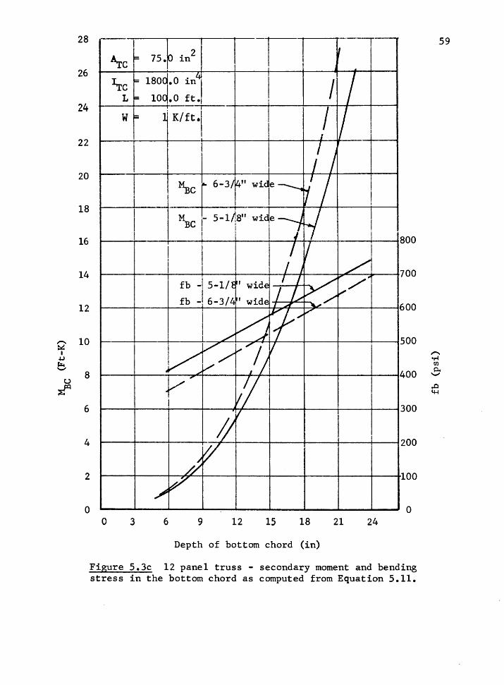
,.... ~ I
.j.J
i::i:.. '-J'
u ~
28
26
24
I 75.~ . 21 I r --i--I
A.re = in .
I.re = 1sod.o in4
I 7 = 1od.o ft. L I
w = 1· K/ft. I I I
I
22
I
I
/ ) 20
18
16
14
12
10
8
6
4
I ~c ... 6-3/ 14" wide---..__. ~I I I I I I I
I MBe - 5-1/,811 wid.,e / lrJ l I i I i
I I
I I I i
/ I I J I I I
~ ..... "
fb -15-1/1 11 wide I I~ L--'/
f b -, 6-3/~ '' wide I .JI -~
I 1' v
~ I _J /
.~/ // I ,/ ,
// I .V
y
// f
I ~
800
700
600
500
400
300
200
2 //
~ ~
100
0 0 0 3 6 9 12 15 18 21 24
Depth of bottom chord (in)
Figure 5.3c 12 panel truss - secondary moment and bending stress in the bottom chord as computed from Equation 5.11.
,.c 4-1
59

60
The moments computed in Table 5.4 are based on the specific top
chord parameters noted on Figures 5.3a,b and c. To account for other
values of A.re and 1Tc' another set of correlations will be developed
to relate the size of the top chord to ~c·
5. 4 ~c AS A FUNCTION OF A.re AND 1tc
Figures 5.4a,b and c relate ~C as a function of A.re and 1tc'
in a manner similar to Figures S.2a,b and c. In this case, the bot-
tom chord is held constant.
The influence of I.re is quite small. Doubling 1tc decreases
M_sc only about 3%. The area, ~C' however, has essentially the same
influence on ~C as did ~c· This is to be expected since the area of
the top chord affects the deflections of the truss nearly the same as
the area of the bottom chord.
As before, we can relate ~C to A.re as follows:
(5 .13)
where ~Cl ~Cl - '\c2 ~C2 =
~Cl - A.:rc2 (5 .14)
and (5 .15)
The computed values of CBl and kBl along with the data used to
compute them are listed in Table 5.5. Letting ~C be defined as the
value of A..rc used when developing the coefficients of E~uation 5.11,
an adjustment factor to adjust Equation 5.11 for a variable ~C can be
developed as follows:

61
TABLE 5.4
COMPUIATION OF ~c USING EQUATION 5.11
8 Panel Deoth b = 5.125 b = 6.75
6 .791317 .894895 7.5 1.340090 1.538890 9 2.080040 2.418210
10.5 3.035920 3.565400 12 4.232140 5.012530 13.5 5.692810 6.791200 15 7.441750 8.932620 16.5 9.502520 11.467700 18 11.898500 14.426900 19.5 14.652700 17 .840500 21 17.788200 21.738500 22.5 21.327700 26.150700 24 25.293700 31.106500
10 Panel Deoth b = 5.125 b = 6.75
6 1.045550 1.168350 7.5 1.722290 1.954270 9 2.613490 3.002310
10.5 3.742280 4.342910 12 5.131200 6.005570 13.5 6.802210 8.019020 15 8.776790 10.411300 16.5 11.076000 13.209700 18 13.720300 16.441200 19.5 16. 730100 20.132000 21 20.125300 24.308000 22.5 23.925300 28.994600 24 28.149600 34.217000
12 Panel Deoth b = 5.·125 b = 6.75
6 1.056760 1.192480 7.5 1.762230 2.019110 9 2.700940 3.132490
10.5 3.900020 4.568210 12 5.385880 6.360880 13.5 7.184390 8.544250 15 9.320820 11.151300 16.S 11.820000 14.214400 18 14.706300 17.765400 19.5 18.003800 21.835300 21 21. 736000 26.455000 22.5 25.926300 31.654700 24 30.597600 37.464300

22
20
18
16
14
12
,.._.,. ~
10 I .., ~ '-"
u 8 ~
6
4
2
0
~ I I
A = ·~s.o in2
BC
~c = 181 >O.O in4
I L = 100 ft. ~
W= 1 K/ft.
I I !
~ r ~c = 2so I ~~c= 800
v I
~c = 1800 I I I
~ I
~ !
~c = 36< ,o~ ~
I I -· I
0 25 75 100 125
Figure 5.4a 8 panel truss - secondary moment in the bottom chord as a function of A.re and I.re·
62

20
18
16
14
12 ,..... ~ I
"'"' 10 µ.. ...._,
t.)
~~ 8
6
4
2
0
63
7~ 2 I ~c= .o in
I -0 in4
~c = 18(
L = 1C 0 ft. ;
w - 1 K/ft. I
-+-I I I
' ) I
~ I=l~ _;; -I = 250
~ ... I = 800
I = 360C ~ ~ I ~
I I
0 25 75 100 125
Figure S.4b 10 panel truss - secondary moment in the bottom chord as a function of A.re and ~c·

24
22
20
18
16
14
12
10
8
6
4
2
0
64
t ~c = 7 .o in2
i-- ·~-T-
1 I = 180
BC +-L = 10 ft. 1------1----+--~-----;-------
w = K/ft. I
0 25 75 100 125
Figure 5.4c 12 panel truss - secondary moment in the bottom chord as a function of A.re and 1i-c·
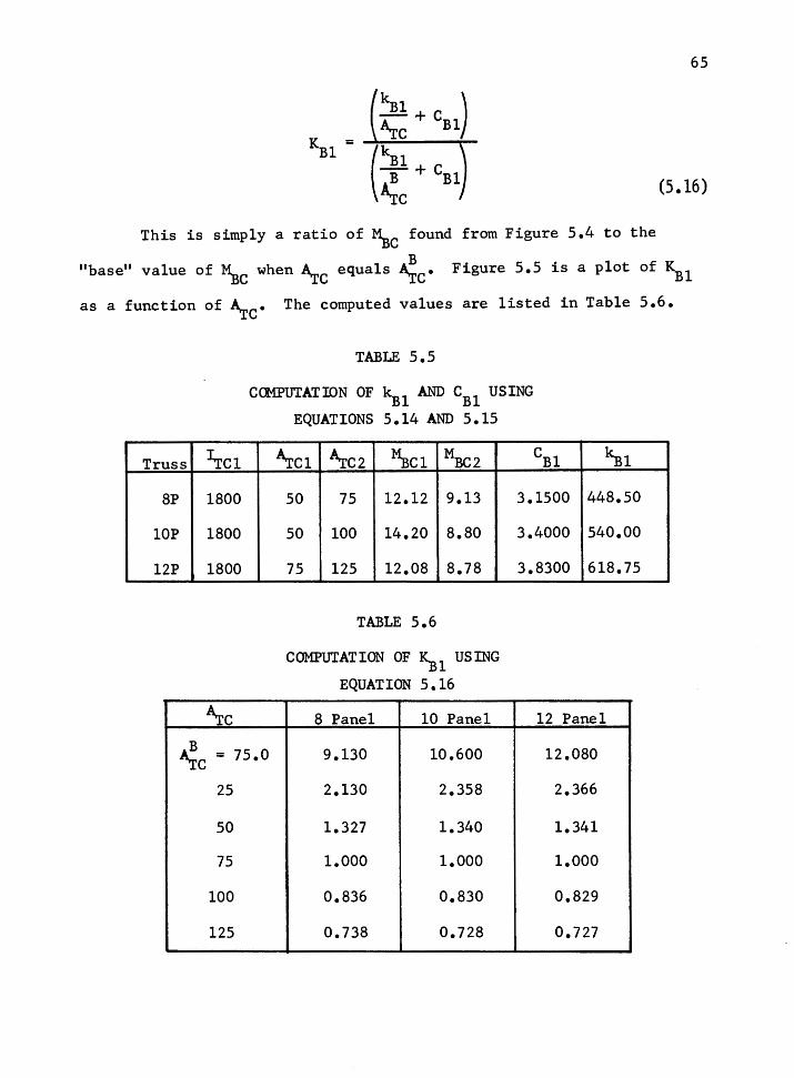
65
(5.16)
This is simply a ratio of ~C found from Figure 5.4 to the
"base" value of ~C when ~C equals ~c· Figure S.S is a plot of KBl
as a function of A.re• The computed values are listed in Table 5.6.
Truss
SP
lOP
12P
~c
~Cl
1800
1800
1800
~c
TABLE 5.5
CCMPUTATION OF ~l AND CBl USING
EQUATIONS S.14 AND S.15
A.rc1 A.rc2 ~Cl MBC2
so 75 12.12 9.13
50 100 14.20 8.80
75 125 12.08 8.78
TABLE 5.6
COMPUTATION OF ~l USING
EQUATION 5.16
CBl
3.1500
3.4000
3.8300
~l
448.50
540.00
618. 75
8 Panel 10 Panel 12 Panel
= 75.0 9.130 10.600 12.080
25 2.130 2.358 2.366
so 1.327 1.340 1.341
75 1.000 1.000 1.000
100 0.836 0.830 0.829
125 0.738 0.728 0.727
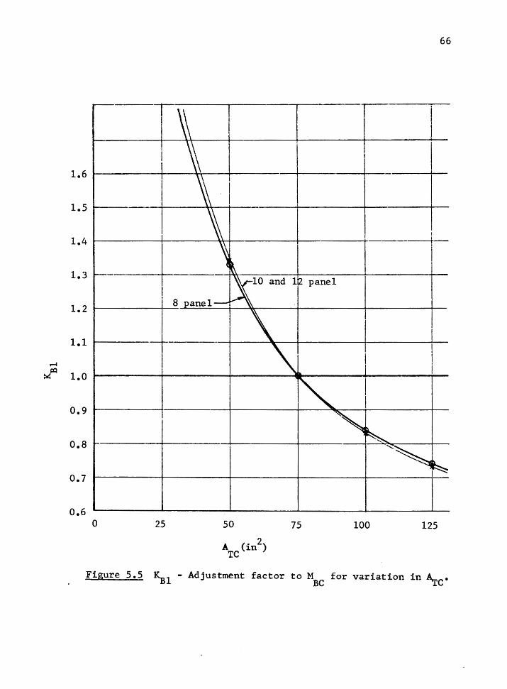
~
~~
1.6
1.5
1.4
1.3
1.2
1.1
1.0
0.9
0.8
0.7
0.6 0 25 50
A (in2) TC
75
66
100 125
Figure 5.5 ~l - Adjustment factor to MBC for variation in A.re·

5. 5 THE EFFECT OF I.re ON THE MOMENT IN THE BCTrTOM CHORD
Though the effect is small, a variation of ~C does influence
~c· Figure 5.6 shows the variation of \c as a function of I.re·
67
Note that the curves for each truss are based on different areas.
variation of ~C between trusses is not of concern at this point.
variation of ~C with 1i-c is what is being considered here.
The
The
The curves of Figure 5.6 appear to intersect the M axis at
finite values. The principal influence of the continuity of the top
chord is to pull some of the load "off" of the truss--that is, it
attempts to act as a beam, carrying some of the load by shear. As
will be shown in the next chapter, the entire top chord of the truss
ends up with positive moments. As can be seen in Figure 5.7, positive
moment at the first top chord joint results in a positive shear in the
end panel. In effect, an upward load equal to the shear is applied to
the truss at the first joint, reducing the axial forces in the members,
thus reducing deflections.
From this it would be expected that the deflection and there
fore the secondary moments will decrease as the stiffness of the top
chord increases. This is indeed the case as was seen in Figure 5.6.
Therefore, the bottom chord secondary moment will be at a maximum but
finite value when ~C equals zero. The same effect will occur in other
types of trusses, even if a net negative moment exists at the joint.
The deflection would still tend to make the moment increase in the pos
itive direction.
Several types of curves can be passed through the points of
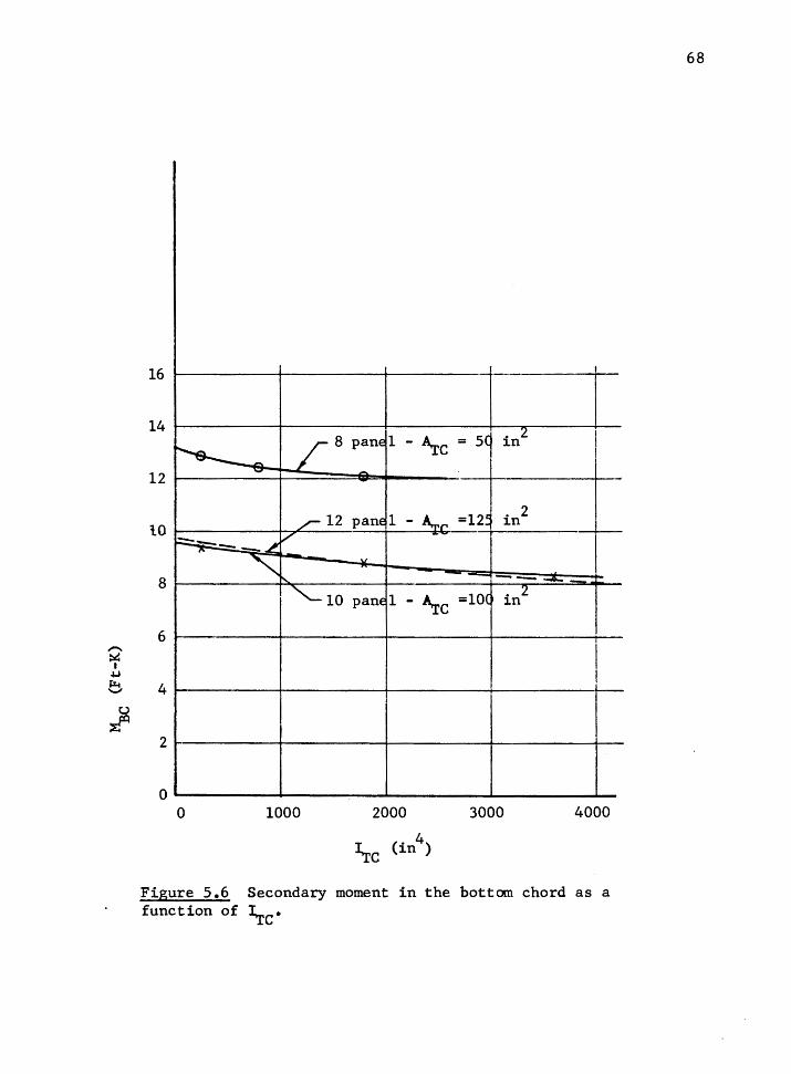
,-... ~ I
.µ ~ .._,
t)
~
16 I I
14
12
/ 8 p:nel - ~C = SC . 2 I
~ in
I
- -
lO
8
,,,,r- 12 pane 1 - A.:~ =12~ in2
I -~~~~ /
"' .,
--... .-.. ........ -"-10 pane 1 - ~c =10( . 2 in
6
I I
4
2
0 0 1000 3000 4000
Figure 5.6 Secondary moment in the bottom chord as a function of ~c·
68
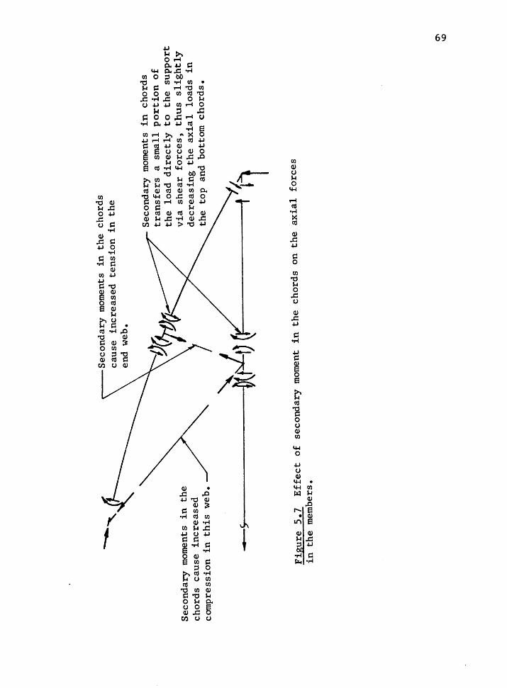
Sec
on
dar
y m
omen
ts
in t
he
cho
rds
cau
se
incre
ase
d
com
pre
ssio
n i
n t
his
web
.
--~-Secondary
mom
ents
in
th
e ch
ord
s ca
use
in
crea
sed
te
nsi
on
in
th
e
end
web
.
Sec
on
dar
y m
omen
ts in
ch
ord
s tr
an
sfers
a
smal
l p
ort
ion
of
the
load
dir
ectl
y t
o
the
sup
po
rt
via
sh
ear
forc
es,
th
us
slig
htl
y
dec
reas
ing
th
e a
xia
l lo
ads
in
the
top
and
bo
tto
m c
ho
rds.
-)rl
t)(r
t
Fig
ure
5
.7
Eff
ect
of
seco
nd
ary
mom
ent
in t
he
cho
rds
on t
he ax
ial
forc
es
in t
he
mem
bers
.
(j\
\0

70
Figure 5.6. A logarithmic curve of the form
M = k ln I + C
can be made to fit quite well over a reasonable bound of I, however
extrapolation could be unreliable since this curve approaches infinity
as I approaches zero, as well as eventually going negative at very
large values of I.
An inverse equation of the form
k M=-+C I
as used before could also be made to fit fairly well, however this
also approaches infinity as I approaches zero. A variation of this
curve, requiring three points to establish, could be written as fol-
lows:
M = ~2 + C (~C + ~2) B2 (5 .17)
This type of curve is plotted in Figure 5.6.
This form of equation meets the requirements of the boundary
conditions and fits the data quite well. Therefore, this form of equa-
tion will be proposed for development of a top chord stiffness adjust-
ment factor, ~2 •
Three points are required to establish this equation, due to
the presence of the three unknown constants.
Three equations can be written:
CB2 = <1tc1 + gB2)MBCl - <1tc2 + ~2)MBC2
~Cl - 1TC2
(5 .18)
CB2 = <~c2 + ~2)?\c2 (~C3 + gB2)~C3
l.rc2 - l.rc3 (5 .19)

71
(5. 20)
Setting Equation 5.18 equal to 5.19, and separating variables,
we obtain:
gB2 = _ [~Cl
where
~Cl - ~C2 1TC2) - qB2 ~C2 ~C2 - ~C3 ~Cl - ~C2) - qB2 (MBC2 - ~C3)
~Cl - 1rc2
~C2 - ~C3 (5. 21)
cB2 an~ kBZ are obtained by substituting gB2 as computed in
Equation 3.21 into Equations 5.18 and 5.20.
Using the value of ITC used in computing ~ and CB of Equation
5.11 as a base value, the following adjustment factor can be proposed:
~2=
(5. 22)
where gB2 can be obtained from <Equation 5.21, ~2 from F.quation 5.20
and cB 2 from ~uation 5.19.
Using data from Figure 5.6, ~2 , ~2 and cB2 are computed in
Table 5.7. Computed values of ~2 are listed in Table 5.8 and plotted
in Figure 5. 8.
5.6 INFLUENCE OF TRUSS SPAN (L) ON ~C
Assuming the same loading intensity per lineal foot, the second-
ary moments will not be affected appreciably. That is, an 80 ft. truss
with 1 K/ft loading will have nearly identical secondary moments to a
100 ft. truss with the same chord sizes and carrying 1 K/ft of load.

Truss
A.rco
ITCl
ITC2
~C3
MBCl
MBC2
~C3
~2
CB2
kB2
TABLE 5.7
COMPUTATION OF ~2 , CB2 AND gB 2 USING
EQUATIONS 5.19, 5.20 AND 5.21
8 Panel 10 Panel
50 100
250 250
800 1800
1800 3600
~c I = 0
250 500 800
1000 1500 2000 3000 4000
12.88 9.39
12.46 a.so
12.12 8.30
993.9914 8796.167
11.51004 5.356620
1704.215 36486 .63
TABLE 5.8
COMPUTED VALUES OF ~2 USING
EQUATION 5.22
8 Panel 10 Panel
800 800
1.061361 1.037757 1.033708 1.025240 1.015309 1.013397 1.000000 1.000000 0.992353 0.991520 0.978601 0.971776 0.969443 0.953857 o. 958005, 0.922576 o. 951147 0.896184
12 Panel
125
250
1800
3600
9.55
8.78
8.14
8184.518
4.589949
41835.64
12 Panel
1800
1.104955 1.087699 1.071437 1.053117 1.041568 1.014783 0.9906284 0.9487978 0.9138334
72
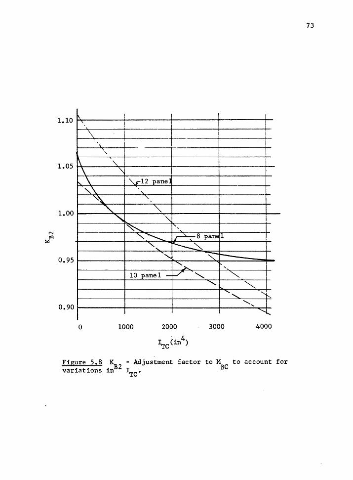
73
I\ I '\. 1.10 . ' '\
' ', ---.---' I \ ' f
'\. !
\ '\ I 1.05
,\ '\.rl2 panel ".\ ' "~
'\. '
1.00 ' """ " .. ·,, I
~ 1"'-',
"~ -, , 8 pane 1 ! .I
""'-, ~~ .....
~ ' :---........
"'>.... ~
'· 0.95
10 panel - ,_/ "'
" """ ..........
"" ..... ....... , . ...........
!"--...
.................
'......... 0.90
0 1000 2000 3000 4000 . 4
~c(in )
Figure 5.8 K - Adjustment factor to M to account for variations inB2
1tc· BC

74
This can be shown by considering the primary factors involved.
As noted earlier, the secondary moments are due to the deflection of
the truss forcing the continuous chords to bend. This deflection is a
function of span, loading, member areas, modulus of elasticity, and to
a small extent the moment of inertia of the chords. Neglecting the
influence of I,
~= f ( 2:~ ) (5. 23)
since P = f (wL)
we have
or, assuming all other parameters constant,
(5. 24)
The moment in the continuous chord is given by the slope deflec-
tion equation as
(5. 25)
Substituting Equation 5.24 into 5.25, we obtain
(5. 26)
which reduces to
(5. 27)
The moment is therefore neither a function of E nor of L.
It can be seen from Figure 5.7 that if M were to remain un-
changed when L is varied, then the shear in the member would be affect-
ed, thus redistributing the axial forces slightly. Therefore, if the

75
influence of I.re and ~C are not neglected, the moment will be slightly
influenced by varying L. This effect will be quite small and will be
neglected in this chapter.
Therefore, the span adjustment factor will be defined in this
chapter as: = 1 (5. 28)
5. 7 THE INFLUENCE OF LOADING ON ~C
The structure has been modeled as a linearly elastic structure;
the effect of changing the magnitude of the uniform load will simply be
linear proportional. Thus, for a uniform load on the top chord,
w ~4 =B
w (5. 29)
Changing the loading pattern, however, will change the deflect-
ed shape of the truss which would have a direct effect on the secondary
moments. Therefore, Equation 5.6 will only be valid for the loading
pattern considered. A separate set of coefficients for Equation 5.6
will need to be developed for each loading pattern desired.
5. 8 THE INFLUENCE OF THE NUMBER OF PANELS ON ~C
Changing the number of panels in the truss changes the struc-
tural configuration, whereas the parameters studied to this point only
changed the member properties. Due to the structural similarity, how-
ever, this parameter can be treated in the same manner as the other
parameters.
Plotting ~C versus the number of panels results in the curve of
Figure 5.9. An equation of the form
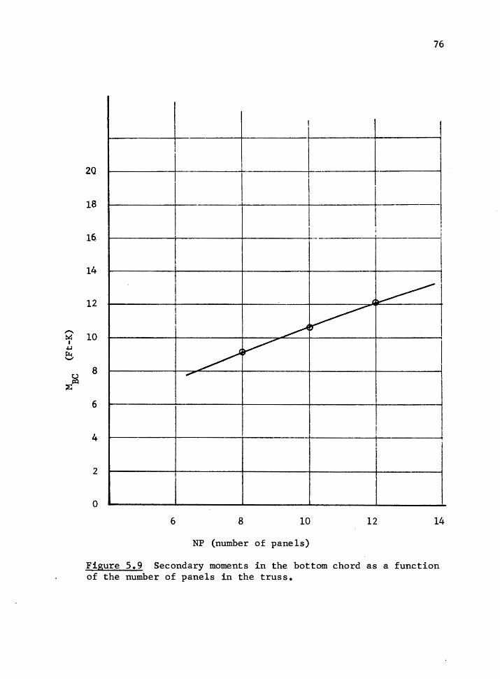
,,....... ~
I .j.J
~ '-'
u ~~
76
20
-i I I
I
I
I
I !
18 -
I
16
14
I I I -- ·-------!
I
12
10
8
I~ I
~ ~ / ~ I
-6
4 I I
I
2
0
6 8 10 12 14
NP (number of panels)
Figure 5.9 Secondary moments in the bottom chord as a function of the number of panels in the truss.

77
~c= ~5
(5. 30)
seems appropriate.
The adjustment factor thus becomes
(5 .31)
The factors for this equation are computed by use of equations
similar to Equations 5.18 through 5.21, replacing ~C with NP. These
computations are summarized in Table 5.9. Values of ~5 are computed
from Equation 5.31, summarized in Table 5.10 and plotted in Figure 5.10.
Note that these values plot as a near straight line function. A sim-
plified equation for ~5 can be written to fit this line. Thus, from
Figure 5.10,
~5 = .33 + .081 NP
TABLE 5.9
DATA FOR FIGURE 5. 9 AND COMPUTATION OF
kBS' CBS AND ~5
Parameter Data Frame Analysis Results
~c = 75 NP1
= 8 ~Cl = 9.13
~c = 1800 NP2 = 10 ~C2 = 10.63
Arre = 75 NP3 = 12 MBC3 = 12.08
I.re = 1800 Com:euted Values of the Constants
kB5 = -10266.0 ~5 = 108.0 CBS = 97.63
(5. 32)
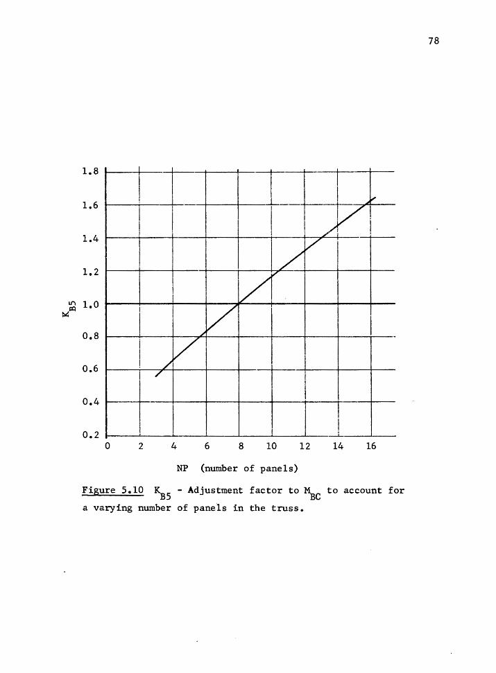
U""I
~~
1.8
1.6
1.4
1.2
1.0
0.8
0.6
0.4
I I
I );' ! .J_ I I
Y1 I I
/ v
i /v
I ~v I -i v I I I ! / I / I
I I I
0.2 I I I -.1.-
0 2 4 6 8 10 12 14 16
NP (number of panels)
Figure 5.10 KBS - Adjustment factor to MBC to account for
a varying number of panels in the truss.
78

TABLE 5.10
COMPUTATION OF ~5
NP KS
4 0.6540
6 0.8299
8 1.0000
10 1.1643
12 1.3231
14 1.4767
16 1.6254
5.9 SUMMARY
The moment in the bottom chord of a bowstring truss with a web
configuration of the types considered in this paper can be computed
from the following equation:
where;
~ = ~oi)i1 i)i2i)i3KB4 l)i5 ( ~c + CB)
1SJo ( ~ + CB) is computed for the 8 pane 1 truss or found from
Figure 5.2a and 5.3a.
KBl is the top chord area adjustment factor which can be
computed from Equation 5.16 using data from Table 5.5
for an 8 panel truss, or taken from Figure S.S.
KB2
is the top chord moment of inertia adjustment factor
from Equation 5.22 using data from Table 5.7 for an 8
panel truss, or taken from Figure 5.8.
79

80
is the truss span adjustment factor, and is taken as 1.0.
is the load intensity factor,
w ~4=l =w
~5 is the adjustment factor for the number of panels in
the truss, computed from Equation 5.31 using Table 5.9
or using the simplified Equation 5.32 or Figure 5.10.
Table 5.11 provides an easy to use summary of the above infer-
mation. Using the data from Tables 5.2 through 5.10, explicit equa-
tions for each factor were computed. These equations are presented
in Table 5.12. Verification of the equations is provided in Chapter
VII.
Coef.
~c
?\co
kB
CB
KBO
N
TABLE 5.11
SUMMARY OF GENERAL EQUATIONS FOR THE BGrTOM CHORD
SECONDARY MOMENTS
General Equation
~co<~OKB1KB2KB3KB4~5)
~ ~C +CB
~Cl ~l - CB)
~Cl~Cl - ABC2~C2 ~Cl - ~C2
(~c r IBCO
ln~C2/MBC1)
ln <I_sc 2/ IBC 1)
EQ. No.
5.6
5.3
s.s
5.4
5.7
5.10
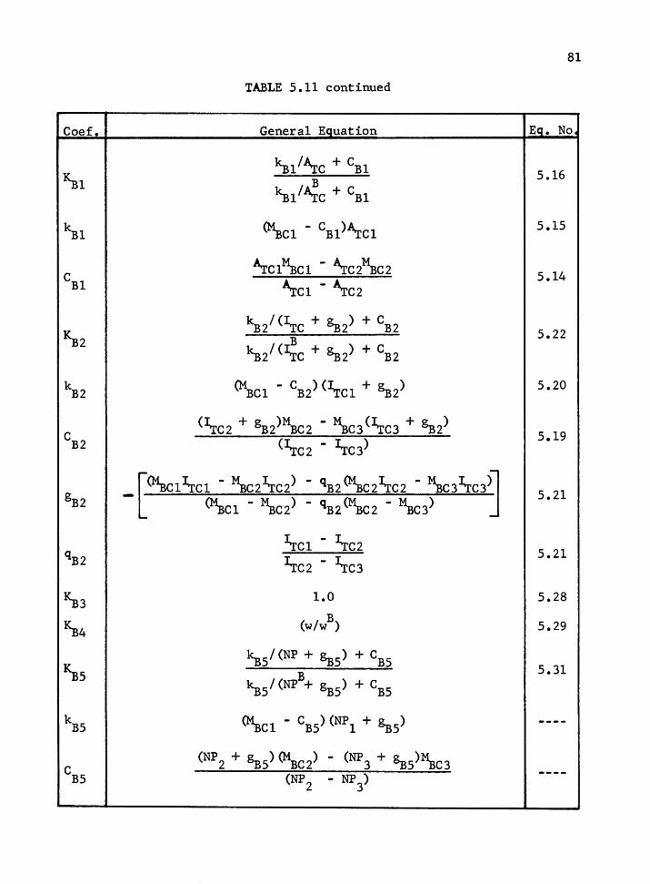
81
TABLE 5.11 continued
Coef. General EQuation Ea. No,
~1 ~i1"rc + CBI S.16 B ~i1ATc + cBl
kBl C?\c1 - CBl)~Cl s.1s
CBI A.rc1~c1 - ~C2MBC2 S.14
~Cl - ~C2
~2 kB/ <1tc + ~2) + CB2
s.22 B ~2/(J:Tc + ~2) + CB2
kB2 (MBCl - CB2)(ITC1 + gB2) s.20
CB2 <I.rc2 + gB2)MBC2 - ~C3 <I.rc3 + ~2)
5.19 <I.rc2 - 1tc3)
gB2 -[<Mac1 l.:rc1 - l\c2l.:rc2> - qB2 <Miic2l.:rc2 - MBc3l.:rc3j
(~Cl - ~C2) - qB2(~C2 - ~C3) s.21
1tc1 - 1tc2 5.21 qB2 1tc2 - 1tc3
~3 1.0 5.28
~4 B
(w/w ) 5.29
~5 ~S/(NP + ~S) +CBS
S.31 B
~S/(NP + gBS) +CBS
kBS C?\c1 - CBS)(NPl + ~5) ----
CBS (NP 2 + gBS) Cl\c2) - (NP 3 + ~s)~C3
(NP2 - NP ) ----3

Coe£.
~5
qBS
Coef.
l\c
?\co
KBO
KBl
KB2
KB3
KB4
KB5
TABLE 5.11 continued
General Eauation
-t~ClNPl - ~C2NP2) - qBsO\czNPz - ~C3NP3)j ~Cl - ~C2) - qB5 <M:sc2 - ~C3)
NPl - NP2 NP2 - NP3
TABLE 5.12
SUMMARY OF EXPLICIT EQUATIONS FOR THE BarTCM CHORD
SECONDARY MOMENTS (BASED ON 8 PANEL TRUSS)
Equation
l\co<KBOKB1KB2KB3KB4KB5)
((450.00)/~c + (12.010))
(I /(3600))(.960343) BC
((49.124)/~c + (0.3450))
((136.78)/(1tc + (993.99)) + (.9238)
1.0
w
((-1124.4)/(NP + (108)) + (10.693)
82
Ea. No.
----
----
CHAPTER VI
SECONDARY MCMENTS IN THE TOP CHORD
The secondary moments in the top chord i.e., the usupport
settlement" type moment resulting from the displacement of the joints,
have the potential of being quite large depending on the values of the
parameters involved. Figure 6.1 shows the moment diagram of the top
chord for an 8 and 12 panel truss for two combinations of parameters.
These diagrams are plotted from data obtained from the computer frame
analyses. For each case, the primary moment has been sub~racted out
of the total moment to provide a plot of the secondary moment for the
respective cases as well.
As can be seen from Figure 6.1, the critical location for the
design of the top chord will be at the first panel point from the end
of the truss, as was the case for the bottom chord. The secondary mo
ment at this location will be designated as M.rc· It should also be noted that the primary moments are generally
small as compared to the secondary moments. The traditional assumption
that the secondary moments are small enough to be neglected, as implied
by the AITC manual, is obviously incorrect. As will be shown by an ex
ample in Chapter X, this assumption can lead to a substantially under
designed structure.

f Truss 1st panel point
Figure 6.la 8 panel truss
Note the small contribution of the primary moment as compared to the secondary moment. The difference between the total moment and the secondary moment represents the primary moments.
I Case 1) t~tal moment I Case 1) second,ry moment -t----_,;:~ I
Heel
Case 2) total moment • --------~ Ca~econdat moment __
i'~ ~--=--
f Truss
Figure 6.lb 12 panel truss
1st panel Heel point
Figure 6.1 Top chord moment diagrams for typical cases.
84

85
6 .1 PARAMETERS AFFECTING M.rc
The principal parameters affecting the secondary moments in the
top chord are the same as those affe.cting the bottom chord, as listed
in Table 5.1.
An additional step must be taken prior to developing the char
acteristic equations and figures if the secondary moments are to be in
vestigated alone. The "primary" moments must first be separated from
the computer g~nerated moments. This is done in Appendix A2, Table
A2.2, using the values of the primary moment computed in Chapter IV.
The ability to predict the moments in the bottom chord in the
10 and 12 panel trusses from the 8 panel datum by use of ~5 (Equation
5.31) was demonstrated in Chapter V. Therefore, only the 8 panel data
will be developed in this chapter, except when developing the ~5 ad
justment factor.
6.2 DEVELOPMENT OF EQUATIONS
Based on the reasoning in Chapter V, the following equation is.
proposed.
(6.1)
The general equations for the individual parameters are present
ed in Table 6.1. The coefficients are calculated in Tables 6.2 through
6.6.
Explicit equations are developed by inserting the coefficients
into the general equations of Table 6.1. These explicit equations are
presented in Table 6.7. Tables 6.8 through 6.12 develop the data re-
86
quired for Figures 6.2 through 6.6.
We thus have the means, by either Table 6.7 or Figures 6.2
through 6.6, for determining the secondary moment in the top chord of
a bowstring truss of 8, 10 or 12 panels with a uniform load on the top
chord.
Figure 6.2, which is analagous to Figure 5.2 for the bottom
chord, represents ~C as a function of A.re and I.re with all other para
meters held constant at the values listed in the figure. Fig. 6.3
transforms this data to represent actual chord sizes and also plots
the bending stress produced by the calculated moment acting on the
given section.
Figure 6.4 provides an adjustment factor to modify the values of
~C and fb obtained from Fig 6.2 or 6.3 to account for a variation in
~c· Figure 6.5 adjusts 11.rc for ~C' and Fig. 6.6 adjusts 11.rc for
trusses with other than 8 panels. Figure 6.6 should be considered
valid only for 8, 10 and 12 panel trusses since other values would re
quire extrapolation beyond the available data. Since NP is not a con
tinuous function, KT5
would more appropriately be taken from Table 6.12.
Figure 6.6 makes it clear however, that increasing the number of panels
in the truss significantly increases the secondary moments which are
induced into the chord.
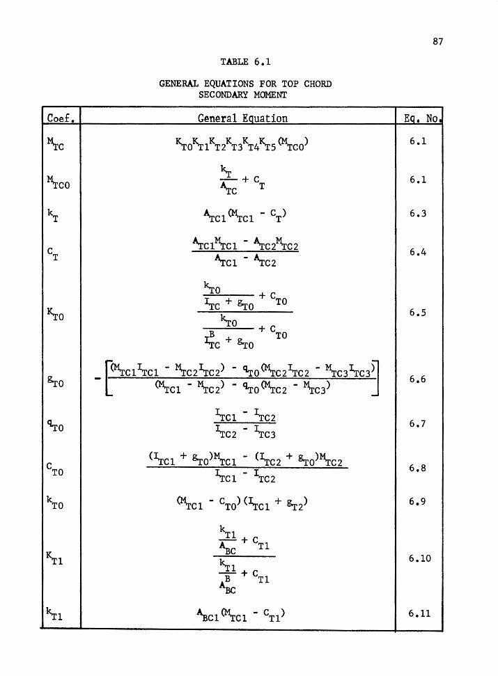
Coe£.
M.rc
M.rco
kT
CT
K.ro
&ro
<Lro
CTO
kTO
KTl
~1
TABLE 6.1
GENERAL EQUATIONS FOR TOP CHORD SECONDARY MOMENT
General Eauation
l<..roK.r1KT2KT3KT4KTS(MTCO)
~ +c A.re T
~Cl CM.rel - CT)
~c1~c1 - A.rc2~c2 ~Cl - ~C2
~o + c ~c + ~o TO
~o B + CTO
1Tc + &.ro
_ [CM.rc1 l.rc1 - ~c2l.rc2) - <Lro CM.rc2l.rc2 - ~c3l.rc3j %c1 - ~c2) - <tro%c2 - ~c3>
~Cl - 1tc2
1tc2 - l.rc3
<I.rc1 + &ro>~c1 - <I.rc2 + &ro>M.rc2
l.rc1. - 1TC2
CM.rel - CTO) (~Cl + ~2)
kTl
~C + CTl
~1 B+ CTl ABC
~Cl ~Cl - CTl)
87
Ea. No.
6.1
6.1
6.3
6.4
6.5
6.6
6.7
6.8
6.9
6.10
6.11

88
TABLE 6.1 continued
Coef. General Equation Eq. No.
CTl '\c1~c1 - '\c2~c2 6.12
~Cl - ABC2
k.r2 + c
K.r2 ~C + &r2 T2
6.13 k.r2
B + CT2 1Bc + &r2
&r2 -t<M.rc1 \c1 - M.rc2
1BC2) - <Lr2 (MTC2
1BC2 - M.rc3l.rc3j
CM.re 1 - M.rc 2) - 'Lr 2 CM.re 2 - M.rc 3) 6.14
<l.r2
1BC1 -
1BC2
6.15 1BC2 -
1BC3
CT2 <~cl + &r2)~c1 - <~c2 + &r2)M.rc2
6.16 ~Cl -
1BC2
k.r2 CM.rel - CT2) (~Cl + &r2) 6.17
l<.r3 1.0 6.18
~4 _J!__
6.19 B w
~5 NP + + CTS
~5 &rs
6.20 k.rs
B + CTS NP + &rs
&rs _ [ CM.rc1NP1 - M.rc2NP 2) - Cl.rs CM.rc2NP 2 - M.rc3NP 3)j
CM.rc1 - M.rc2) - Cl.rs CM.rc2 - 1\-c3) 6.21
Cl.rs NPl - NP2
6.22 NP2
- NP3

Coef.
CTS
kT5
TABLE 6.1 continued
General Equation
(NPl + Srs)~Cl - (NP2 + &rs)M.rc2 NPl - NP2
<Mi:rc1 - CTS)(NPl +&rs)
TABLE 6.2
COMPUTATION OF ~ AND CT FOR
AN 8 PANEL TRUSS USING EQUATIONS 6.3 AND 6.4
Designation 1 12TC02 Designation 2 12TC12
~co = 1800
A.rc1 = so
A.rc2 = 75
~Cl = 12.80
l\ic 2 = 9.78
CT = 3.7400 ~ = 453.00
TABLE 6.3
COMPUTATION OF k.ro, CTO AND Sro FOR
AN 8 PANEL TRUSS USING EQUATIONS 6.6, 6.7, 6.8 AND 6.9
Designation 1 12TCOO Designation 2 12TC01 Designation 3 12TC02
1rc1 = 250 ~Cl= 2.10
~C2 = 800 M.rc2 = 6.02
~C3 = 1800 ~C3 = 12.80
&ro = 30,011.s CTO = 221.70 ~o = -6,645,492.8
89
Eo. No.
6.23
6.24
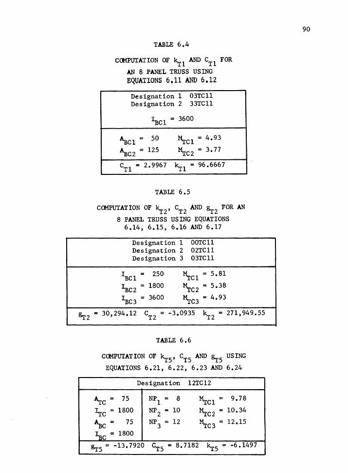
TABLE 6.4
COMPUIATION OF ~l AND CTl FOR
AN 8 PANEL TRUSS USING EQUATIONS 6.11 AND 6.12
Designation 1 03TC11 Designation 2 33TC11
~Cl = 3600
~Cl= 50 M.rcl = 4.93
~C2 = 125 M.rc2 = 3.77
CTl = 2. 9967 ~l = 96.6667
TABLE 6.5
COMPUIAT ION OF kT 2, CT 2 AND ~ 2 FOR AN
8 PANEL TRUSS USING EQUATIONS 6.14, 6.15, 6.16 AND 6.17
Designation 1 OOTCll Designation 2 02TC11 Designation 3 03TC11
IBCl = 250 ~Cl = 5.81
~C2 = 1800 ~C2 = 5.38
~C3 = 3600 ~C3 = 4.93
&:r2 = 30,294.12 CT 2 = -3.0935 kT2 = 271,949.55
TABLE 6 .6
COMPUIATION OF ~5 , CT5 AND ~5 USING
EQUATIONS 6.21, 6.22, 6.23 AND 6.24
Designation 12TC12
A.re = 75 NP = 1 8 M.rc1 = 9.78
I.re = 1800 NP = 2 10 M.rc 2 = 10. 34
~c= 75 NP = 3 12 ~C3 = 12.15
~c = laoo
~5 = -13. 7920 s 5 = 8.1182 ~5 = -6.1497
90
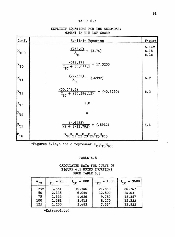
Coef,
M.rco
KTO
KTl
~2
~3
~4
~5
~c
TABLE 6.7
EXPLICIT EQUATIONS FOR THE SF.cONDARY MOMENT IN THE TOP CHORD
Exolicit Eauation
<4~~0) + (3. 74)
-519,179 1Tc + 30,011.5 + 17.3233
<2~~55 ) + (.6992)
(50,548. 2) + (-0.5750) !BC + (30,294.12)
1.0
w
(-.6288) NP+ (-13.792) + (• 8912)
~0~1~2~3~41<.r5~co
*Figures 6.la,b and c represent ~0K.r5~CO
Arre 25* 50 75
100 125
TABLE 6.8
CALCULATED DATA FOR CURVE OF FIGURE 6.1 USING EQUATIONS
FROM TABLE 6.7
~c = 250 ~c = 800 ~c = 1800
3.651 10.340 21.860 2.138 6.054 12.800 1.633 4.626 9.780 1.381 3.912 8.270 1.230 3.483 7.364
*Extrapolated
~c = 3600
86.747 24.03 18.357 15.523 13.822
91
Fi~re
6.la* 6.lb 6.lc
6.2
6.3
6.4

Depth
6 7.5 9
10.5 12 13.5 15 16.5 18 19.5 21 22.5 24
TABLE 6.9
CALCULATED DATA FOR FIGURE 6.2 BASED ON THE EQUATIONS FROM TABLE 6.7
5.125 Wide 6.75 Wid~
~c f b ~c f b
1.07831 420.804 1.12114 332.189 1.68606 421.105 1.79003 339.443 2.48152 430.398 2.67095 351.731 3.47394 442.673 3.77643 365. 369 4.67062 455 .671 5.11492 378.883 6.07545 468.327 6.68973 391.534 7.6883 480.05 8.49798 402.867 9.50446 490.454 10.5303 412.575
11.5145 499.273 12.7709 420.441 13.7042 506.319 15.1977 426.321 16.0552 511.466 17.7834 430.135 18.5452 514.643 20.4967 431.865 21.1489 515.826 23.3036 431.548
TABLE 6.10
CALCULATED VALUES OF l<.rl
1tc = 1800
~c = 75
~c = 1800
~c l<.r1 25 1.601 50 1.15 75 1.00
100 0.925 125 0.880
92

93
TABLE 6.11
CALCULATED VALUE OF ~2
~c = 1aoo ~c= 75
~c= 75
~c ~2 200 1.083 400 1.072 800 1.051
1200 1.030 1600 1.010 1800 1.000 2000 0.9903 2400 o. 9711 2800 0.9525 3200 0.9342 3600 0.9134
TABLE 6.12
CALCULATED VALUES OF ~5
NP ~5
8 1.000 10 1.057 12 1.242

22
20
18
16
14
12
10 ,...... ~ I ~ µ...
8 .._,, C,)
~ 6
4
2
0
94
0= computer data
6.2 and 6.5
.--~~~-+-~~~~-+-~·~~-+-~~~~+-~~~--4-
0 25
" "
75
~c = 18 o
---I
-- -- ~ -----4-·- ---
100 125
Figure 6.2 8 panel truss - secondary moment in the top chord as a function of "Tc and I.re·
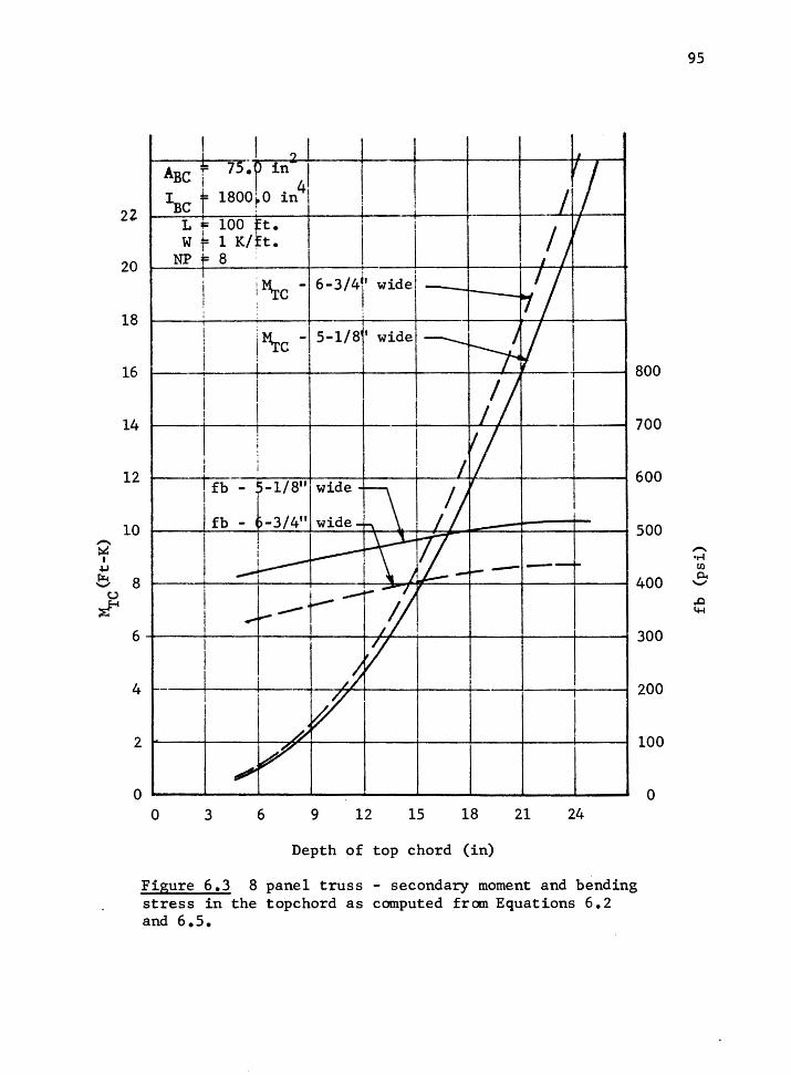
22
20
18
16
14
12
10 ,,..... ~ I
.µ ~ 8 .......,
u ~
6
4
2
0
_I 2 I ABC f 1 ·f in I 1800~0 in
41 1
BC t L *= 100 tt· I
1 K/. t. w r= NP 8
iM.rc 6-3/41' wide
JM.re -15-1/8' : I
800
700
600 f b - -1/ 811
! f b - -3/411 wide 500
I I I I
400
300
- 200
100
0 0 3 6 9 12 15 18 21 24
Depth of top chord (in)
Figure 6.3 8 panel truss - secondary moment and bending stress in the topchord as computed from Equations 6.2 and 6.5.
95
,,..... •r-1 en p.. .......,
..0 4-1

..-f
~
N
~
1.6
1.5
1.4
1.3
1.2
1.1
1.0
0.9
0.8
0.7
0.6
1.10
1.08
1.06
1.04
1.02
1.00
0.98
0.96
0.94
0.92
0.90
.
\ \
' ' ""-'-~
0 25 75 100
Figure 6.4 i<.rl - Adjustment factor to ~C to account for
variation in ~c·
' ' ' ~ ~ "' ' " "~
" ~ ' 0 1000 2000 3000 4000
Figure 6.5 J<T 2 - Adjustment factor to ~C to account ~c
for variation in ~c·
96
-
125
5oog = (in )

1.25
1.20
1.15
1.10
1.05
1.00
0.95
0.90
8 10
NP (number of panels)
12
I I
Figure 6.6 ~5 - Adjustment factor to l\ic to account for a
variation in the number of panels in the truss.
97
CHAPTER VII
VERIFICATION OF EQUATIONS DEVELOPED IN CHAPTERS V AND VI
In order to check the equations developed in Chapters V and VI,
the equations of Tables 5.12 and 6.7 were written into a small computer
program. Computation of ~C and ~C were made for each combination of·
parameters for which a frame analysis had been run. The results were
compared with the values of M C and M obtained from the frame analy-B TC
sis runs.
Table 7.la compares the moment in the bottom chord as computed
by the equations developed in Chapter V (Table 5.12) denoted by "M BC
equation" against the moment obtained from the frame analysis denoted
by "M computer". The column labeled "Ratio" lists the ratio of the BC
two, that is
~C equation Ratio =
~C computer
Table 7.lb compares the secondary moment in the top chord in a
similar fashion.
It can be seen that the equations generally predict the moments
with 1% or 2%. A few cases have up to nearly a 10% discrepancy.
This range of accuracy is considered quite acceptable. The
bending stress resulting from the secondary moments is generally in the
range of 20% of the allowable bending stress. Therefore, a 10% error

99
in computing the moment will result in only a 2% error in the combined
stress equation which is well within accepted engineering accuracy. In
addition, it will be seen in Chapter VIII that bolt slippage in the web
to chord joints can reduce the secondary moments by as much as 60% in
some cases, which further justifies the acceptability of the accuracy
obtained.
The cases which showed the greatest discrepancy were in the
most part unlikely combinations of parameters, such as case 12TC30
which has the following parameters:
~c = 75
A.re = 125
~c = 1800
\.c = 250
Greater accuracy would likely have been obtained if the para
meters used to develop the various constants had "bounded" the range
of data. This was not always done which results in some extrapolation
being required.
Chapter IX will present a systematic approach to choosing para
meters and developing characteristic equations which greatly simplifies
and improves reliability over the techniques used to develop the equa
tions of Chapters V and VI.
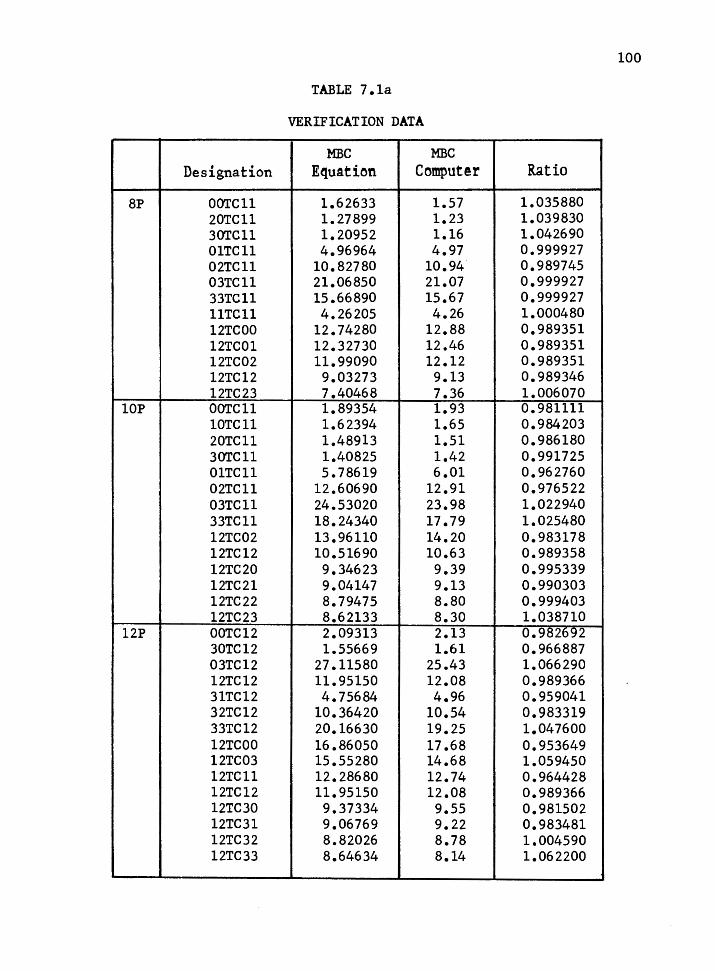
100
TABLE 7.la
VERIFICATION DATA
MBC MBC Designation Equation Comput!r Ratio
BP OOTCll 1.62633 1.57 1.035880 20TC11 1.27899 1.23 1.039830 30TC11 1.20952 1.16 1.042690 OlTCll 4.96964 4.97 0.999927 02TC11 10.82780 10.94 0.989745 03TC11 21.06850 21.07 0.999927 33TC11 15.66890 15.67 0.999927 llTCll 4. 26205 4.26 1.000480 12TCOO 12.74280 12.88 0.989351 12TC01 12.32730 12.46 0.989351 12TC02 11.99090 12.12 0.989351 12TC12 9.03273 9.13 0.989346 12TC23 7.40468 7.36 1.006070
lOP OOTCll 1.89354 1.93 o. 981111 lOTCll 1.62394 1.65 0.984203 20TC11 1.48913 1.51 0.986180 30TC11 1.40825 1.42 0.991725 OlTCll 5. 78619 6.01 o. 962760 02TC11 12.60690 12.91 0.976522 03TC11 24.53020 23.98 1.022940 33TC11 18.24340 17.79 1.025480 12TC02 13.96110 14.20 0.983178 12TC12 10.51690 10.63 0.989358 12TC20 9.34623 9.39 0.995339 12TC21 9.04147 9.13 0.990303 12TC22 8.79475 8.80 0.999403 12TC23 8.62133 8.30 1.038710
12P OOTC12 2.09313 2.13 0.982692 30TC12 1.55669 1.61 0.966887 03TC12 27 .11580 25.43 1.066290 12TC12 11.95150 12.08 0.989366 31TC12 4. 75684 4.96 0.959041 32TC12 10.36420 10.54 0.983319 33TC12 20.16630 19.25 1.047600 12TCOO 16.86050 17.68 0.953649 12TC03 15.55280 14.68 1.059450 12TC11 12.28680 12.74 0.964428 12TC12 11. 95150 12.08 0.989366 12TC30 9.37334 9.55 0.981502 12TC31 9.06769 9.22 0.983481 12TC32 8.82026 8.78 1.004590 12TC33 8.64634 8.14 1.062200

101
TABLE 7.lb
VERIFICATION DATA
MTC MTC Designation Equation Computer Ratio
BP OOTCll 5.59679 5.810 0.963303 20TC11 4.46999 4.640 0.963359 30TC11 4.24463 4.400 o. 964688 OlTCll 5.44508 5.650 0.963731 02TC11 5.18257 5.380 0.963303 03TC11 4.74908 4.930 0.963303 33TC11 3.60172 3.770 0.955364 llTCll 4. 71424 4.900 o. 962090 12TCOO 2.07127 2.100 0.986321 12TC01 5.87251 6.020 0.975500 12TC02 12.44710 12.800 0.972430 12TC12 9.51037 9.780 0.972430 12TC23 15.05110 15.400 o. 977344
lOP OOTCll 5.91733 6.160 o. 960606 lOTCll 5.12311 5.250 0.975830 20TC11 4.72599 4.790 0.986638 30TC11 4.48773 4.510 0.995062 OlTCll 5.75693 5.910 0.974101 02TC11 5.47939 5.510 0.994444 03TC11 5.02108 4.890 1.026800 33TC11 3.80800 3.610 1.054850 12TC02 13.16000 13.820 0.952242 12TC12 10.05510 10.340 0.972442 12TC20 1.41488 1.130 1.252110 12TC21 4.01150 3.890 1.031230 12TC22 8.50259 8.560 0.993293 12TC23 15.91310 16.060 0.990854
12P OOTC12 14.73810 15.467 0.952871 30TC12 11.17740 11.670 0.957790 03TC12 12.50580 12.700 0.984708 12TC12 11.81560 12.150 0.972474 31TC12 10.87440 11.270 0.964900 32TC12 10.35020 10.630 0.973675 33TC12 9.48444 10.080 0.940917 12TCOO 2.57332 2.610 0.985948 12TC03 28.94210 28.460 1.016940 12TC11 5.57455 5.900 0.944838 12TC12 11.81560 12.150 0.972474 12TC30 1.48047 1.630 0.908261 12TC31 4.19744 4.400 0.953963 12TC32 8.89670 8.970 0.991829 12TC33 16.65070 16.070 1.036140

CHAPI'ER VIII
arHER FACTORS AFFECTING THE SECONDARY MOMENTS IN THE CHORDS
In addition to the primary factors listed in Table 5.1 which
affect the secondary moments in the chords, there are several other
influencing factors. These factors, though not treated as "primary"
factors, can have significant effect. Some of these factors include:
1. Web joint slippage 2. Heel fixity of the bottom chord 3. Heel bolt slippage 4. Center line bottom chord splice fixity/slippage
The effects of these parameters are briefly treated in the fol-
lowing sections.
8. 1 BOLT SLIPPAGE IN THE WEB CONNECTIONS
Bolt slippage in the web to chord connection allows significant
relief of the induced moments. The effect of bolt slippage was simu-
lated by reducing the area of the webs in a single step iteration in
order to approximate a 1/16 in. to 1/8 in. slip displacement. This
procedure was discussed in section 3.2.S.l. Table 8.1 provides a com-
parison of the maximum moment in the top and bottom chord for a few
cases with and without the simulated joint slippage. The colunms
labeled % represent the ratio
with slip * lOO% without slip

103
As can be seen, for the range of parameters considered, the bot-
tom chord moment is reduced from 30% to 60%, with the average reduction
being approximately 44%. The top chord moment is likewise reduced from
40% to 60% with the average reduction about 50%.
This is a very brief study, so no conclusive recommendations can
be made at this time. It does appear, however, that a 30% reduction
could be safely assumed for the bottom chord and a 40% reduction for
the top chord.
In general, the combinations which result in large moments gen-
erally appear to have the greater reduction when joint slippage is per-
mitted.
MBC Designation No Slip
8 Panel
OOTCll 1.57 12TC12 9.13 33TC11 15.67
10 Panel
OOTCll 1.93 03TC11 23.98 30TC11 1.42 33TC11 17.79
TABLE 8.1
EFFECT OF BOLT SLIPPAGE IN WEB CONNECTIONS
~c ~c With Slio % No Slip
1.06 67.5 8.02 5.27 57.7 11.99 8.37 53.4 5.98
1.31 67.9 7.87 11.37 47.4 6.60 o.85 59,9 6.22 6.92 38.9 5.32
8.2 HEEL FIXITY
~c With Slio %
4.76 59.4 5.42 45.2 3.33 55.7
4.17 53.0 3.22 48.8 2.79 44.9 2.18 41.0
If the heel column connection is such that any degree of fixity
is imposed on the bottom chord, significant moments will be introduced

104
into the bottom chord. The heel design shown in Figure 2.7, which has
had considerable usage, has the potential for this problem when the
colunm is large.
The moment at the end of the truss might be computed simplistic
ally as R x e where e is the eccentricity based on member center lines.
In reality, however, the probable stress distribution shown in Figure
8.1 would result in a moment of R x e' where e' is the more probable
eccentricity based on reaction force lines.
Regardless of the actual moment, it will affect the bottom chord
as shown in Figure 8.2. The moment transfered to the first joint will
be additive with the deflection induced moment based on a pinned heel
joint. This increase in moment can be seen in Figure 8.3 where the mo
ment in the bottom chord based on output from computer analysis of the
8 panel truss is plotted. The conditions shown represent the boundar
ies i.e., fully fixed versus a purely pinned connection.
In the actual structure, complete fixity is highly unlikely.
The maximum moment achievable would be equal to Rx e', which would
most likely be less than the "fixed" moment.
The amplification of the moment at the first joint, which is al
ready the critical point, suggests that care should be taken to avoid
eccentric heel connections in these trusses. The connection detail of
Figure 2.7 should therefore be avoided in favor of a detail similar to
that shown in Figure 2.6.
8.3 BOLT SLIPPAGE IN THE HEEL CONNECTION
As discussed in section 3.2.S.2, bolt slippage was simulated by

105
/ /
/ /
,,/ .,,,,,
PTC .,,,,,
/ / / - -
~ --/
--";'
PBC
~ - -L---- -- -- --
M = Rx e' R e
Figure 8.1 Probable stress distribution in an eccentric heel.
Moment for concentric heel\_ -----
~c
Amplified moment at first panel point due to eccentric heel
P x e'
Heel 1st panel point
2nd panel point
Figure 8.2 Amplification of moment in the bottom chord due to an eccentric heel.

,.... ~ I ~ e
t,;)
~
106
30
20
10
0
-10
-20
-30 -+-I Heel 1st panel
point 2nd panel
point 3rd panel of
point ~ truss
Figure 8.3 Effect of a fully fixed heel on the bottom chord moment in an 8 panel truss with bolt slippage permitted in the web connections.

107
reducing the area of the "rigid" link that was modeled into the heel of
the truss (see Figure 3.1). The area was reduced an amount necessary
to increase the axial deformation of that element by 1/8 in.
In most cases, several bolts ·are required in this connection.
The change of slippage occurring is therefore thought to be small. In
a design that contains only a few bolts or otherwise allows for signi-
ficant movement in the joint, consideration should be given to the
effects of this possibility.
Bolt slippage in this connection has the adverse effect of in-
creasing the secondary moment in both top and bottom chords by a signi-
ficant amount. The brief study made in this investigation indicates
that a 1/16 in. joint slip will increase the moments by an amount equal
to approximately
M= .16EI
R2
where ~ is the length of the end bottom chord panel (i.e., J. = L/7 for
an ·a panel truss).
Translated into bending stress, for a rectangular section, this
becomes
fb = .08Ed
~2
For a 100 ft. truss with a 13-1/2 in. deep chord, a 1/16 in.
joint slip will induce approximately 70 psi of additional bending into
the chord. This represents an approximate 16% increase in bending
stress for this case.

108
8.4 BOTTOM CHORD SPLICE
The effect of joint fixity and joint slippage in the center line
splice is negligible. The effect at the end pArtal joint, Yhieh has
been shown in Chapters V and VI to be the critical location on the
chord, is nominal and appears to be of little concern in terms of in
duced stresses.
8. 5 TERTIARY (P-/::J.) MCJ:1ENTS
If the bottom chord is fabricated nearly straight, it will be
forced into a slightly curved shape when the truss is loaded. Ter
tiary, or P-/::J., moments will result from the tension acting on the cur
ved member.
This possibility was considered briefly in order to determine
if this was of serious concern in the design of the trusses.
For the cases considered, the moment in the bottom chord was
found to be amplified by 2% to 9%, which represents less than a 1%
change in the unity equation.
This does not appear to be of enough significance to be of con
cern in the design. This is especially true when·considering the fact
that the truss is normally fabricated with a camber in it. Under maxi
mum loading, the bottom chord is expected to be nearly straight. For
these reasons, no further consideration has been given to the tertiary
moments in the bottom chord.
When considering tertiary moments in the upper chord, we are
dealing with the P-/::J. moments resulting from the axial load acting

109
through the change of curvature of the chord. The moment resulting
from the original eccentricity of the chord has been accounted for in
the primary moment analysis (see Chapter IV).
Tertiary moment in the upper chord would only be considered cri
tical if the curvature increased under load, thus amplifying the origi
nal eccentricity. As was made clear in Chapter VI, however, the upper
chord, due to secondary moment (i.e., support settlement type moments
caused by the downward joint deflections) is subject to positive moment
(compression on top) along its entire length. Therefore the curvature
will be decreased slightly which will result in the tertiary moments
tending to decrease the total moment. This slight advantage should
conservatively be neglected in the author's opinion.
In light of the above discussion, tertiary moments were not
studied any further.

CHAPTER IX
DEVELOPMENT OF A SYSTEMATIC APPROACH TO THE DESIGN OF STANDARD STRUCTURES
9.1 INTRODUCTION
To this point our approach has been to start with a mass of
data and proceed to develop a series of characteristic equations from
that data by which to design a structure. The complexity and tedious-
ness of the ensuing equations with their multitude of variables and co-
efficients cry for a systematic approach which can be applied to a
structure in a productive way.
This chapter will attempt to develop such a method. In develop-
ing and implementing such a method, three questions must be considered.
1. What degree of accuracy is required or desired? 2. What analytic tools are available to the analyst/designer? 3. Is the problem being considered a single use design case
or is it a standard structural configuration being developed?
A general method will be outlined here which can be applied to
a range of situations for structures of varying types. From that point,
a specific approach will be developed for the design of timber trusses,
with emphasis being placed on the design of continuous glu-lam chords
of bowstring trusses.
9.2 GENERAL CHARACTERISTIC EQUATION CONCEPT
The design of a statically indeterminate structure using a
111
computer for analysis normally proceeds in an iterative method. A
structural configuration is developed for which initial trial sections
are chosen for the members. The structure is then modeled and the re-
quired input data entered into the computer.
At this point an analysis is made of the trial design using a
standard analysis program. The computed forces and moments are used to
check the chosen members for adequacy or oversizing. This may be done
by hand, or by the computer if a more extensive design program is avail
able. New sizes are then selected and the process repeated until a
satisfactory design is obtained.
This basic iterative technique is certainly valid and indeed de
sirable when good engineering judgment is incorporated into the process.
No proposal is made here to change the iterative process.
The most serious drawback to the iterative process is the ex-
pense and time requirement for running many analysis iterations, par-
ticularly for standard structures such as trusses. The use of inhouse
terminals and an interactive program such as GTSTRUDL(6) or the availa
bility of an inhouse computer with interactive capabilities goes a long
way to reduce the extensive time periods associated with overnight batch
processing. The cost of working interactively is expensive, however.
This is of particular concern when dealing with "standard"
structures because the client, such as a truss manufacturer, may need
the design "that afternoon" to prepare a bid. Even with single use
problems, the number of iterations is often kept small in order to save
cost and time. A "that is good enough" design is used rather than try
ing a few more refinements or alternatives in an effort to optimize the

112
structure.
The attempt then, will be to reduce the number of analyses re
quired. A specific set of analysis runs will be made, from which "char
acteristic equations" of the structure can be developed. Sufficient
runs must be made in order to provide the data required for developing
the equations. Thus, the use of the large computer is not eliminated.
For a single use project, the development of the characteristic equa
tions may not be justified, since nearly as many iterations may be re
quired in many cases. For the standard structure, or for a structure
in which many iterations are desired for optimization, the use of the
characteristic equations can be of significant usefulness.
A proposed procedure would be to use a large computer, such as
through a service bureau, to analyze a specific set of "designs" to pro
vide a data base. The section properties need not represent any actual
member sizes and therefore eliminate the need for an "initial" design.
The data base can then be transfered to a small microcomputer, or even
a programmable calculator, for the development of the characteristic
equations.
An iterative technique can then be performed using the "charac
teristic equations" to develop the design or designs. Note that struc
tural dimensions can be included as a parameter in the development of
the equations. This would be quite useful for "standard structures",
such as trusses, in which span and loading intensity may vary over a
wide range.
One must begin then, by selecting the parameters that are to be
varied. This will be a judgment decision based on many factors which

113
will be tempered by the answers to the three questions asked earlier.
In addition, the type of structure will have a marked influence on the
decision. For example, a low rise moment frame with no bracing will be
only marginally affected by axial de'formations. Therefore, one may
wish to vary the I values only and not refine the equations to account
for varying the areas. In multistory frame, one may choose to have all
beams of the same section for fabrication economy. Therefore, the beam
I's do not need to be varied individually, but as a whole. Similar
reasoning is usually applied to the design of columns in buildings.
One would most likely consider changing section at every two floors for
example.
In truss designs, both area and moment of inertia have a signifi
cant impact on the induced moments. Therefore, both A and I should be
varied. However, the chord dimensions would most likely remain con
stant throughout the truss, so once again only a few parameters must
be varied.
The desired degree of accuracy will also affect the decision.
For example, if a particular parameter is expected to only affect the
results by 4% or 5%, it may not be worth the effort to include that
parameter in the equations.
The availability and cost of the computer will also have an im
pact on the number of parameters to be varied and the number of points
to be used to develop the equations. In general, the more parameters
to be varied, the more computer runs necessary.
It should be noted that the "characteristic equations" need not
be "exact" equations, and in many cases would not be. Their function

114
is to provide numbers which can be used as a guide in designing the
structure. Once developed, the equations should be back checked to
test their reliability. For a single use problem, this would entail
making a final frame analysis computer run using the proposed final de-
sign as a check on the design. For a standard structure, a typical de-
sign or even arbitrary properties could be used in a few runs to check
the results.
Once the parameters to be studied are chosen, the input for the
computer runs must be logically selected to provide a usable data base.
The following procedure is proposed.
1. Select a "base" value for each parameter. 2. One run should be made with all "base" values. 3. All runs should utilize the "base" parameters except
for the particular parameter being varied.
Three points are required to establish a curve which will reason-
ably represent the structure. The "base" run will provide one of these
points for each parameter. For many parameters, one of the points can
be determined inductively from an understanding of structural behavior.
Specifically, often one can determine if the function will approach
zero or infinity as the value of the parameter goes to zero. If this
is the case, then two of the three points are established and only one
additional run need be made. If the limit is not zero or infinity, an
additional run must be made in order to describe the curve.
9.3 PARAMETERS TO BE VARIED
The possible parameters to be varied can be more than just the
area or moment of inertia of a member. The span or other dimensions,

115
modulus of elasticity, Poisson's ratio, temperature effects, web stiff-
ness (which would allow for the inclusion of joint slippage), and nearly
any other quantity that is part of the model input data might be varied.
For each parameter selected to be varied, two computer runs will be re-
quired. Thus, the importance of a parameter should be considered care-
fully before selecting it as a variable.
It was shown in Chapter V that it is possible to correlate the
effect of the number of webs in the truss (8 panel, 10 panel, 12 panel,
etc). Thus, to an extent, even the structural configuration itself can
be varied.
9.4 DEVELOPMENT OF A GENERAL CHARACTERISTIC EQUATION
In general, it has been found that an equation of the form
k y = + c
x + g (9.1)
can be used to describe the variation of a variable (y), such as the
moment at a specific point, with respect to the variation of a specific
parameter (x).
In Equation 9.1,
y = variable being considered x = the parameter being varied (such as the area of
the top chord, for example) k,g and C are constants which define the curve for
the specific parameter.
Since there are three unknown constants involved, three data
points (or "boundary conditions") are required to determine them, as
discussed previously.
Three data points, to be obtained from the computer runs, may be

defined as follows:
x1
= lower limit of the parameter
x2
= base value of the parameter
x3
= upper limit of the parameter
y1
y2
& y3
= the value of the variable obtained from the computer run associated with x1 , x 2 and x 3 cases.
Thus, Equation 9.1 may be written as
k Y1 = + + C xl g
k y 2 = x2 + g + C
k + c Y3 = x3 + g
Combining Equations 9.2 and 9.3,
therefore,
k =[ 1 y 2 - y 3 1 ]
(x2 + g) (x3 + g)
or,
(
y - y ) k = x: - x~ (x2 + g)(x3 + g)
Similarly, combining Equations 9.3 and 9.4,
Combining Equations 9.5 and 9.6,
116
(9. 2)
(9.3)
(9.4)
(9.5)
(9.6)

or,
( :: : :~ ) ( ~ ~ : ~ ~ ) = (:~ : : )
Let B = ( :: ~ :~ ) ( : ~ - : ~ ) then
g =
or g = x - x /B
3 1 l/B - 1
C can be written as
k c = y - ~-------2 (x
2 + g)
In general
117
(9.7)
(9.8)
(9.9)
(9.10)
(9.11)
where all x 'I: xi are constants taken as their respective "base" values.
This equation can be normalized by dividing yB {the value of y
for the case where all x =base values). Thus, a coefficient
is obtained.
y. f (x.)
Ki = ~ = ~ y y
A separate coefficient is obtained for each parameter, x1•
We can now write n
y. = YB TI (Ki) J i=l
(9 .12)
(9 .13)

n where TI represents the cumulative product of K
1 through Kn.
i=l
118
An equation such as 9.13 will be obtained for each variable, y.
Thus, by denoting y as subscripted y , and defining the 11 base11 value of j
B y. as Y., we obtain J J B n
Y. = (Y.) TIK .. J J i=l l.J
Using Equation 9.1 for f(x), we obtain
or,
n y. = (Y~) II
J J i=l
k .. l.J c
+ + .. x. g. . l.J 1 11
y~ J
y. = (Y~51-n) n ( k!; + c. ·) J J • 1 x. g.. 1J
i= l. l.J
(9 .14)
(9.15)
It must be noted at this point that Equation 9.15 is not an
exact equation. It assumes that all of the data curves are of the form
of Equation 9.1 which in some cases will be inaccurate. In most cases,
the error is believed to be small for values of x between x1
and x3
•
The error may become appreciable, however, if the curves are extrapo-
lated beyond the limits of x1
and x3
• It is therefore important to
choose x1
and x3
as expected minimum and maximum values for the para-
meter.
If more than one loading pattern is to be analyzed, a set of
equations for Y. will be obtained, with one equation for each loading J
pattern. The further subscript R will be added toy, Y, k, g, and C,
with ~ going from 1 to p, therefore
(9 .16)

9.4.1 Swmnary
The implementation of the method is summarized below.
I. DATA BASE PREPARATION
1. Select the structural configuration.
2. Select all parameters (x .) to be varied (e.g. 1
area of top chord of a truss).
3. Select "base" values for each parameter (xi2) •
The base values should preferably be a medium
value from the expected range of possible values
for the parameter.
4. Select minimum and maximum expected values for
each parameter (xil and xi3 respectively).
5. Using base values for all parameters, analyze the
structure for each loading case utilizing a stand-
ard frame analysis computer program.
6. Two additional computer runs will be required for
each parameter for each loading case as follows:
For each loading case:
For i = 1 to n
a. All "base" values except change xi to xi1•
b. All "base" values except change xi to xi3
•
II. DEVELOPMENT OF CHARACTERISTIC EQUATIONS
1. Study the results from the frame analysis made in
part I. Determine the location of the critical
points in the structure which will or potentially
can govern the design of the members and/or
119

connections, such as the point of maximum moment.
2. With the information above, select the "vari-
ables" (y .. ) to be studied. These might be l.JR
the moment at the critical location, axial loads,
shear, reactions, deflections or other results
120
which are of concern to the designer. Results which
are not affected by varying any of the parameters
need not be included at this point.
3. Obtain the values of the variables from the out-
put files of the frame analysis made in part I,
B (y ijR' y ijlR' and y ij3R) •
4. Compute the constants of Eq. 9.16 for each vari-
able (j) for each parameter (i) for each load case
(~). The constants are kijj (from Eq. 9.5), gij~
(from Eq. 9.9) and C .. (from Eq. 9.10). l.JQ
5. Save the values of the constants for use in the
design process.
III. VERIFICATION OF EQUATIONS AND THE DESIGN PROCEDURE
A. VERIFICATION OF EQUATIONS
1. Once the constants for Eq. 9.16 are com-
puted, Eq. 9.16 can be used to compute
the values of the variables (i.e., maximum
moment, etc.) for any combination of para-
meter values (e.g., A, I, etc.) the designer
selects for the specific design.
2. If design data for a standard structure is

121
being developed, such as for a specific truss
type, the characteristic equations should be
checked by running a complete frame analysis
for a few typical designs until the designer
is confident that the equations predict the
values of variables within acceptable preci
sion. Once the equations are verified, step
III.B.l can be used repeatedly by simply enter
ing the values of the parameters into Eq. 9.16
for each variable and checking the design in
the usual iterative process.
3. If the problem is a one time solution situa
tion, the final design obtained from step
III.B.l can be checked by a complete frame
analysis using the final design values of the
parameters.
B. DESIGN PROCEDURE
1. The traditional iterative design process is
used, except Eq. 9.16 is used in place of run
ning a complete frame analysis for each itera
tion. Trial values of each parameter are se
lected and the values of the variables (i.e.,
moment in bottom chord, etc.) are computed
using Eq. 9.16. The adequacy of the members
as well as other considerations such as de
flections are checked and adjustments ma.de to

the trial sizes. This procedure is repeat
ed until a satisfactory design is obtained.
9.5 COMPUTER IMPLEMENTATION OF THE PROCEDURE
122
This procedure can be easily programmed into a microcomputer to
make the process nearly completely automatic. The procedure is highly
interactive, quick and inexpensive, which allows the designer to try
several combinations of parameter values in developing the design.
To demonstrate and test the procedure, a program was written
for use on a microcomputer. The program is written in the Microsoft
Basic language and is listed in Appendix 4. The program actually con
sists of three programs, corresponding to the three sections of the
summary. The first program enters the parameter and variable names and
the base and extreme values of the parameters, corresponding to steps
I.2,3 and 4. The program then sets up combinations of parameters to
use in the frame analysis, according to steps I.5 and I.6 of the summary.
At this point, the structure would be modeled for the frame ana
lysis and the runs would be batch processed (steps I.5 and 6). Once the
data is obtained from the series of frame analyses, a second program de
velops the characteristic equations and automatically saves the con
stants on disc files.
This data is then available for use by program number three
which uses the characteristic equations (i.e., Eq. 9.16) to compute the
value of each variable ~C' ~C' etc.) for the set of parameter values
specified by the designer during the interactive process of using pro
gram three. This corresponds to step III.B.l of the summary. Program
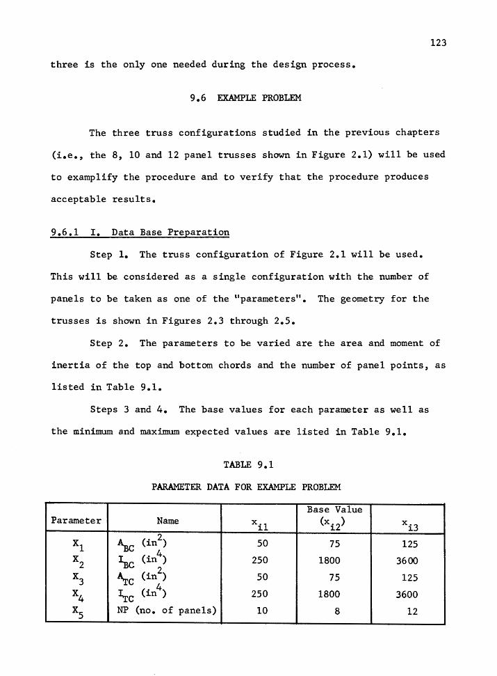
123
three is the only one needed during the design process.
9.6 EXAMPLE PROBLEM
The three truss configurations studied in the previous chapters
(i.e., the 8, 10 and 12 panel trusses shown in Figure 2.1) will be used
to examplify the procedure and to verify that the procedure produces
acceptable results.
9.6.1 I. Data Base Preparation
Step 1. The truss configuration of Figure 2.1 will be used.
This will be considered as a single configuration with the number of
panels to be taken as one of the uparameters". The geometry for the
trusses is shown in Figures 2.3 through 2.5.
Step 2. The parameters to be varied are the area and moment of
inertia of the top and bottom chords and the number of panel points, as
listed in Table 9.1.
Steps 3 and 4. The base values for each parameter as well as
the minimum and maximum expected values are listed in Table 9.1.
TABLE 9.1
PARAMETER DATA FOR EXAMPLE PROBLEM
Base Value Parameter Name xil (xi2) xi3
xl ~c (in2) 50 75 125
x2 ~c (in4) 250 1800 3600
x3 A.re (in2) 50 75 125
X4 ~c (in4) 250 1800 3600
XS NP (no. of panels) 10 8 12

124
Step 5. At this point a computer frame analysis would be run
using "base" values for all parameters. For this example, data al
ready obtained in previous work will be utilized. Since the values of
the parameters used in this earlier work (i.e., Chapters V and VI) were
not selected using the structured format that this procedure utilizes,
appropriate values will be computed using the characteristic equations
developed in Chapters V and VI.
Step 6. Two additional computer runs would be made for each
parameter. In our case, having five parameters, ten additional runs
are required. Each run will utilize "base" values for all parameters
except for the specific parameter being studied which will be changed
to xil or xi3• As mentioned in step five, however, previously acquired
data will be used in this example.
Program number one (see Appendix A4) is designed primarily to
interactively enter the parameter data (Table 9.1) into the computer
for use by the second and third programs. In addition, it produces an
organized list of required combinations of computer runs to be made in
steps I.5 and I.6.
The second program is now used to compute the constants (k, g
and C) for the characteristic equations.
9.6.2 II. Development of the Characteristic Equations
Step 1. The output from the frame analysis computer runs are
now studied in order to determine the critical points in the structure.
As was found in previous chapters, the critical point for designing the
top and bottom chords occurs at the first panel point in from the end

125
of the truss.
Step 2. We will therefore select the moment at the top chord at
the critical location <Mi:rc = Y2
) and the critical moment in the bottom
chord ~C = Y1
) as our variables. The axial load has only minor vari
ation and therefore will not be considered a variable in this example.
Step 3. The values of the variables (i.e., ~C and ~C) are now
extracted from the frame analysis output listings. In our case, as
mentioned before, the data is obtained from the characteristic equa-
tions of Chapters V and VI. This data is listed in Table 9.2. It
should be noted that this data is not truly accurate since it is ob-
tained from the approximate characteristic equations. For this reason,
TABLE 9.2
OUTPlIT DATA FOR THE CHOSEN VARIABLES (OBTAINED FRCM COMPlITER FRAME ANALYSIS)
Case Y l = MBC (Ft-K) y2 = M.rc (Ft-K)
Base* 9.13 9.78
~Cl ** 10.64 11.00
~C3 7.58 a.so
~Cl 1.35 10.42
~C3 17.60 8.83
"rc1 11.94 12.80
~C3 6.57 7.20
l.rc1 9.41 1.65
~C3 8.68 18.20
NPl 10.63 10.34
NP3 12.08 12.15
*Computer run using all parameter "base values.
** Computer run using2all "base" values except setting ~C equal to ~Cl (=50 in in this case).

this example problem will produce less accurate results than would
otherwise be obtained. The equations of Chapters V and VI are accu-
rate enough, however, that the results should be reasonable.
Step 4. Compute the constants kij
and cij (Eq. 9.10).
(E q • 9 • 5) , g . . l.J
(Eq. 9.9)
Effects of ~C (i=l) on ~C (j=l) for Load Case 1 ( =1).
From Table 9.1,
from Table 9.2,
using Eq. 9.9,
y1
= 10.64, y2
= 9.13, y3 = 7.58
= x3 - xl/B l/B - 1
where
B m = ( :: - : ~ ) ( ~ ~ : ~ ~ ) = (i ~5 - -5~ 5 ) (
9.13 - 7.58 ) 10.64 - 9.13
= o.513245
the ref ore
= ( 125 - 50/ .513245 ) glll 1/.513245 - 1 = 29.0816
using Eq. 9.5
km = ( :~ ~ :~ ) (xl + gm) (x2 + gm)
= ( 107~4--5~· 13 ) (50 + 29.0816)(75 + 29.0816)
the ref ore
klll = 497.149
126

127
Using Eq. 9.10
( 497 .149 ) -= 9.13 - 75 + 29.0816 - 4.35347
The constants for all other combinations of i, j and t are com-
puted in the same fashion. This is done automatically by the second
computer program (see Appendix A4). The computed values of kijR' giji
and C .. for this example are listed in Table 9.3. l.J~
Step 5. The constants computed in the previous step are saved
for use in the design process using Eq. 9.16.
9.6.3 III.A. Verification of Equations
At this point, in a typical situation, a few frame analyses
would be run using an actual loading and typical member sizes. Ac-
tually, these runs could be made at the same time as the other cases
were run. The characteristic equations (Eq. 9.16) are used to compute
the values of each variable using the same parameter values of the test
case. If satisfied that the computed values are within acceptable accur-
acy, the equations can now be used to design structures.
In our example, all of the computer runs used in Chapters V and
VI will be used to test the results of the equations. The computed
values are listed along with the actual (as computed by the frame analy-
sis program) values in Table 9.4.
Program three computes MBC and M.rc using Eq. 9.16. ~C for case
"OOTCll" (See 3.2.6 for explanation of the case designation.) will be
calculated by hand to demonstrate the procedure. All other cases are

TABLE 9.3
CONSTANTS FOR THE "GENERAL CHARACTERISTIC EQUATIONS" FOR THE BOWSTRING
TRUSS EXAMPLE PROBLEM
Input Data Constants
"ec:BASE. l ): q.ll 8 ( l ' l ' l ~: .513245 6 ( l f l I l l = 29. 181&
"TC~B~SE, l )• 9.78 K ( l , l ' l ): 497.14, (( 1 ' l ' 1 }: 4.35347
"BC'.~BC l LD l >= tt.64 "TC<HBC l lD 1 l• il B< 2 I l ' 1 ): .q37482 61 2 ' 1 ' l ): 4qq94,7
~BC·ABC 2 LD l l• 7.58 kl 2 , l , 1 1a-l.3tS73E~t1 c ( 2 , l '
"TC'.~ac 2 LD t != e.s ~BC;IBC 1LD1 >= 1.35 B< l , 1 ' 1 ): ,455516 6( l ' l ' 1 l= 12.7451 "rcqec 1 LD l la lt.42 k( 3 ' l , 1 }: 618.827 C< l , 1 , l l • 2.li745 ~ac:1sc 2 LD t >• 17.o "TCilBC 2 LD 1 l= 8.Bl 8( 4 • l , 1 ): 1. 38393 6! 4 ' 1 ' 1 l=-12325.6 "BC•ATC 1 LD 1 ): 11.94 K ( 4 , 1 , l I= 22%1. 4 C< 4 , 1 , 1 J• 11.3114 ~TC{ATC 1 LD ! l= 12.8 ~BC(AT~ 2 ~D l )• 6.57 8 ( s ' l ' 1 l: • q93333 6( s ' l ' 1 ): 118 "TC(AT~ 2 LD 1 Js 7.2 Kl S , l , 1 l=-1t2b6 c ( s ' l ' l ) = 97. b20~ ~BCmc l LD l }: 9.41 "TCiITC 1 LD 1 )• 1.65 B ! l , 2 , l l = • 52•591 6 ( 1 ' 2 ' 1 ) = 32. 7588 ~~Ct!iC 2 LO 1 ): B.oe K ( l , 2 I 1 l = 435. 198 C( l , 2 , l ): 5.74131 "TC(!TC 2 LD 1 )z 18.2 "~C :NP 1 LD 1 l= ~I.bl 8( 2 ' 2 ' 1 ): l.27821 6( 2' 2' 1 !=-l~b41.1 "TCiNf 1 LD l l= 11.34 K( 2 I 2 ' 1 ): 87%f.4 c ( 2 ' 2 ' 1 ) = lb.1l5 "BC:NP 2 LD i J= 12.tB "TC\NP 2 LO 1 ): 12.15 8( 3 I 2 ' 1 ): • 4~7153 &l 3, 2, 1 ): 5.9241H
(( 3 I 2 f l ) : 540. 717 C< l , 2 , 1 >= 3.12427
8( 4 ' 2 ' i 1= .sq1e21 6( 4 ' 2 ' 1 ): 273~8.~ K( 4 , 2 , 1 )•·4.225SBE•f6 C( 4 , 2 ,
I ( 5 , 2 , 1 l • 2. 11 bl7 6( s , 2 , 1 )=-13. 1n l( 5, 2, 11•-6.14n C( 5, 2, 1 l= 8.71824
128
1 i= 2bt.276
l }: 154.646
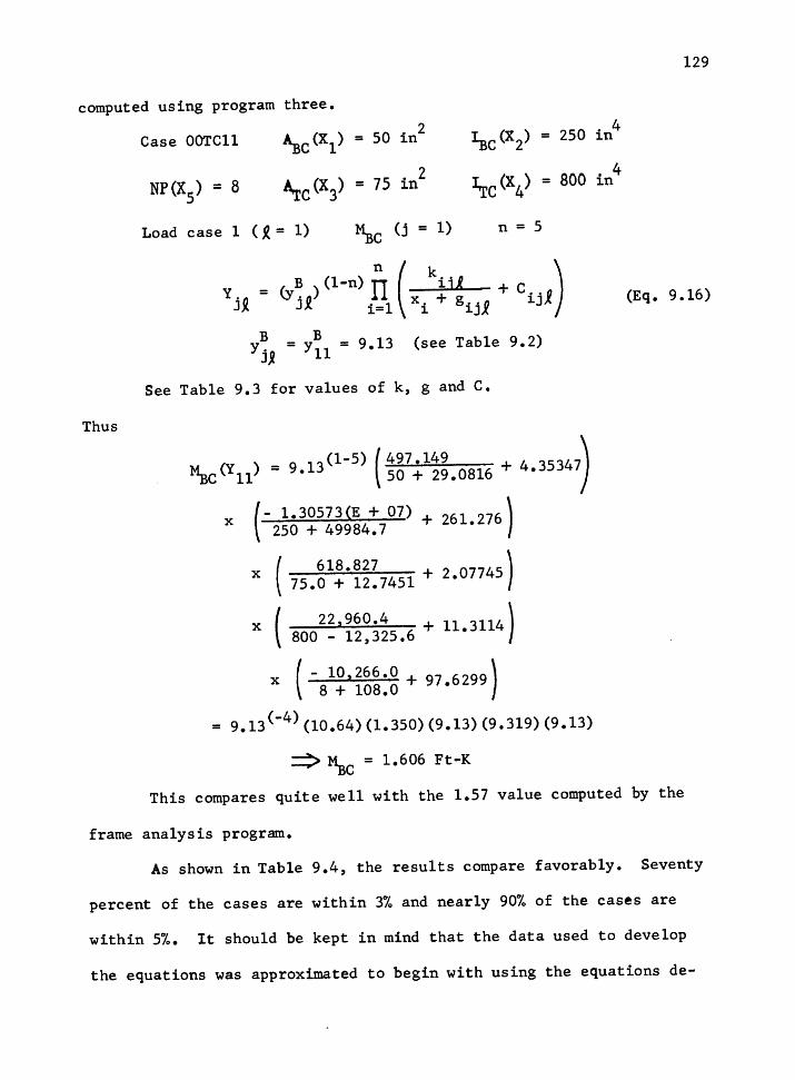
129
computed using program three.
Case OOTCll ~C(Xl) = 50 . 2 ~C(X2) 250 . 4
in = in
NP(X5) = 8 A.re (X3) = 75 in2 lrrc (X4) = 800 in4
Load case 1 ( R. = 1) ~c (j = 1) n = 5
(Eq. 9 .16)
Thus
(see Table 9.2)
See Table 9.3 for values of k, g and C.
- (1-5) ( 497 .149 ) ~C(Yll) - 9•13 50 + 29.0816 + 4 •35347
x (- l.30573(E + 07) + 261 276 ) 250 + 49984.7 •
x ( 75.~1!·~;~ 7451 + 2.07745)
x ( 2 2 2 96 0• 4 + 11 3114 ) 800 - 12,325.6 •
x ( - 10,266.0 + 97 6299) 8 + 108.0 •
= 9.13(-4)(10.64)(1.350)(9.13)(9.319)(9.13)
:::::::> ~C = 1.606 Ft-K
This compares quite well with the 1.57 value computed by the
frame analysis program.
As shown in Table 9.4, the results compare favorably. Seventy
percent of the cases are within 3% and nearly 90% of the cases are
within 5%. It should be kept in mind that the data used to develop
the equations was approximated to begin with using the equations de-

130
veloped in Chapters V and VI. The original data did not bound the
range of parameter values in all cases. Thus, some of the data was
based on extrapolation. It would be expected then that the use of
original, accurate data to develop the characteristic equations would
produce very reliable results. The results should be more than accu-
rate enough in light of the discussions in Chapter VIII.
8 Panel
OOTCll~* 20TC11 30TC11 OlTCll 02TC11 03TC11 33TC11 llTCll 12TCOO 12TC01 12TC02 12TC12 12TC23
10 Panel OOTCll lOTCll 20TC11 30TC11 OlTCll 02TC11 03TC11 33TC11 12TC02 12TC12 12TC20 12TC21 12TC22 12TC23
TABLE 9.4
GENERAL CHARACTERISTIC EQUATION VERIFICATION DATA
~Cle Actualt Actual t
~c Ratio ~c" ~c
1.606 1.57 1.02 5.557 5.81 1.239 1.23 1.01 4.557 4.64 1.144 1.16 0.99 4.294 4.40 4.955 4.97 1.00 5.444 5.65
10.860 10.94 0.99 5.216 5.38 20.937 21.07 0.99 4.709 4.93 14.916 15.67 0.95 3.639 3. 77 4.252 4.26 1.00 4.840 4.90
12.306 12.88 0.96 2.160 2.10 12.188 12.46 0.98 6.069 6.02 11. 940 12.12 0.99 12.800 12.80
9.130 9.13 1.00 9 .. 780 9.78 7.193 7.36 0.98 15.233 15.40
1.865 1.93 0.97 5.876 6.16 1.600 1.65 0.97 5.224 5.25 1.438 1.51 0.95 4.817 4.79 1.328 1.42 0.94 4.540 4.51 5.753 6.01 0.96 5.756 5.91
12.645 12.91 0.98 5.514 5.51 24.308 23.98 1.01 4.979 4.89 17.317 17.79 0.97 3.847 3.61 13.901 14.20 0.98 13.533 13.82 10.630 10.63 1.00 10.340 10.34 9.079 9.39 0.97 1.460 1.13 8.992 9.13 0.98 4.104 3.89 8.809 a.so 1.00 8.654 8.56 8.375 8.30 1.01 16 .106 16.06
Ratio
0.96 0.98 0.98 0.96 0.97 0.96 0.97 0.99 1.03 1.01 1.00 1.00 0.99
0.95 1.00 1.01 1.01 0.97 1.00 1.02 1.07 0.98 1.00 1.29 1.06 1.01 1.00

TABLE 9.4 continued
Actual Actual 12 Panel ~c MBC Ratio ~c ~c Ratio
OOTC12 2.082 2.13 0.98 14.56 15.47 0.94 30TC12 1.483 1.61 0.92 11. 251 11.67 0.96 03TC12 27.139 25.43 1.07 12.338 12.70 0.97 12TC12 12.080 12.08 1.00 12.150 12.15 1.00 31TC12 4.575 4.96 0.92 11.022 11.27 0.98 32TC12 10.029 10.54 0.95 10.560 10.63 0.99 33TC12 19.334 19.25 1.00 9.534 10.08 0.95 12TC00 16.282 17.68 0.92 2.683 2.61 1.03 12TC03 15.019 14.68 1.02 29.592 28.46 1.04 12TC11 12.330 12.74 0.97 5.761 5.90 0.98 12TC12 12.080 12.08 1.00 12.150 12.15 1.00 12TC30 S.959 9.55 0.90 1.509 1.63 0.93 12TC31 8.873 9.22 0.96 4.241 4.40 0.96 12TC32 8.693 8.78 0.99 8.945 8.97 1.00 12TC33 8.264 8.14 1.02 16.646 16.07 1.04
* As.computed from Eq. 9.16 using the computer program of Appendix 4.
t From frame analysis.
"*1l"Frame analysis computer run designation (see section 3.2.6 for description).
9.6.4 III1 B. Design Procedure
131
The equations are now ready to be used to aid in the design of
a structure. The traditional iterative procedure is used, using the
characteristic equations to compute the values of the variables rather
than running full frame analyses.
For our example, a 100 ft., 8 panel truss with the configuration
shown in Figure 2.3 will be designed to carry 930 lb/ft. on the top
chord using AITC-117-79(5) and the 1982 NDS specifications.
Use 5-1/8 in. wide, combination number 3 glu-lam for the chords.

132
Top Chord: From Figures 4.4 and 4.5,
_ ( 100 ft ) ( 9 3 o 1 b If t ) = pmax - 96 •79 100 ft 1000 lb/ft 90.0 K
and
M.rc (primary) = 2.21 { 1~~g) = 2.06 Ft-K (at first joint from the end)
Bottom Chord: The tension in the bottom chord can be obtained
from a stress diagram or from the canputer frame analysis runs. For
our example, T = 84.4 K at the first joint.
Initial trial,
5-1/8 x 12 bottom chord 5-1/8 x 10-1/2 top chord
Program three is executed. The following parameter values are
entered when requested:
ABC = 61.5 in2
A.re = 53.8 in2
~c = 738 in4
lrrc = 494.4 in 4
NP = 8
The following results are obtained from the program:
M = 4.94 Ft-K BC
M.rc = 3.84 + 2.06 = 5.90 Ft-K
Allowable stresses for combination number 3 (from AITC 117-79,
Table 2):
6 E = 1.8(10 ) psi
Fb = 2000 psi xx
Ft = 1450 psi Fe = 2300 psi
15% increase for snow load
The members will be checked against the "unity" equations of the
NDS~7 ) section 3.10, for combined flexural and axial loading.

Top Chord:
(x - x axis)pe!d = (13.l ft)(l2 in/ft)/(10.S in)
= 14.97 > 11
1800 K = 0.671 J FEc = 0.671 (x - x axis) (2.3) (1.15)
= 17.50
11 < Rid< 17 .S, therefore use intermediate column equation
' [ (2 /d) 4] Fc(x-x) = Fe 1 - 1/3 -i--
= 2, 3 (1.15) [1 - 1/3 (i~:;6) ~ = 2.173 Ksi
J = g,d - 11 x K - 11
14. 97 - 11 = 17 .so - 11
= 0.611
Determine allowable bending stress:
n = l.92n = 1.92(2.0 ft)(l2 in/ft) Xe Xu
= 46.1 in
therefore,
c = J 46 • 1 ( 10• 5) = 4. 2 9 2 < 10 s (S.125) 2
therefore,
' Fb = Fb = 2.0(1.15) = 2.30 Ksi xx
133
NPS Ref Section
3. 7. 3 .1 (b)
3.7.3.l(b)
3.10.2.l
3.3.3.4
3.3.3.4

therefore,
( ld2) 1/9 < 1
CF =
CF = 1.0
fc = 90.0K/53.8 in2 = 1.673 Ksi
fb = (5.90 ft-K)(l2 in/ft)/(94.17 in3) = 0.752 Ksi
Unity equation (x-x axis)
f~ + f~ < 1 Fe Fb - J f c
x x
1.673 0.752 2.173 + (2.30 - (0.611)(1.673))
= 0.770 + 0.589 = 1.36 >> 1.0 No Good
Although this member is not adequate, we will
also check the unity equation considering buckling
about the y-y axis in order to demonstrate the
method used in subsequent calculations which are
computed using a documented programmable calculator
program. (8)
Rcy-y)/d = (2.0 ft)(l2 in/ft)/5.125 in= 4.68 < 11
therefore,
' Fe =Fe = 2.30(1.15) = 2.65 Ksi yy
therefore, the unity equation becomes:
--¥- + f~ ~ 1 Fe Fb
yy
= 1.673 + 0.752 2.65 2.3
134
NDS Ref Section
3.10.2.1
3.10.2.2
= 0.63 + 0.33 = 0.96 Ok
For the second iteration, try a 5-1/8 x 13-1/2
BC and a 5-1/8 x 12 TC.
The following parameters are now used in the
characteristic equations (we will use the computer
program):
~c = 69.2 . 2 ~c 1050.8 in4 in
A.re 61.5 in 2 1Tc 738 in4 = =
The following results are obtained:
M = 6.07 Ft-K BC
M.:rc = 4.82 + 2.06 = 6.88 Ft-K
NP =
The calculator program yields the following
results for the top chord:
8
(x-x axis): 0.62(axial) + 0.37 (bending) = 0.99<1.0
(y-y axis): 0.55 + 0.29 = 0.85 < 1.0 Ok
Now check the bottom chord.
Assume a connector at the joint to consist of
a 3/4 in. diameter bolt with two 4 in. shear plates.
Ac (= Projected Area of the connector) = 8.29 in2
therefore,
Net Area = 69.2 - 8.29 = 60.9 in2
ft = 84•4 K = 1.386 Ksi 60.9 in
2
135
NDS Ref Section
fb = (6.88 Ft-K)(l2 in/ft) = o. 530 Ksi
155.7 in3
Since ft is much larger than fb, only the bot-
tom face of the member will be checked. The top
face will not be subjected to bending compression
buckling, which can occur if the bending stress
dominates.
Thus, the unity equation becomes:
ft (net) + fb ~ 1 Ft Fb
= 1.386 + 0.530 1.45(1.15) 2.0(1.15)
= 0.83 + 0.23 = 1.06 > 1.0
The next trial will use a 5-1/8 x 12 TC and a
5-1/8 x 15 BC.
~c = 76.88 in2
~c = 61.50 in2
~c = 1441.4 in4
~c = 738.0 in4
NP = 8
The computer program yields the following re-
sults:
~C = 7.916 Ft-K.
~C = 4.60 + 2.06 = 6.06 Ft-K
Using the calculator program,
Bottom chord: 0.74 + 0.21 = 0.96 < 1.0 Ok
Top chord: 0.62 + 0.32 = 0.94 < 1.0 Ok
136
NDS Ref Section
3.10.1
137
Therefore, a 5-1/8 x 12 TC and a 5-1/8 x 15 BC would provide an
adequate structure. Referring to Chapter VIII, however, it was suggest
ed that a 30% reduction in bending moments caused by secondary effects
would be reasonable due to bolt slippage in the web connection. If the
designer chooses to take this into account, the second trial, using a
5-1/8 x 13-1/2 BC and a 5-1/8 x 12 TC could be considered an accept
able design. The unity equation for the bottom chord would become:
0.83 + (.7)(0.23) = 0.99<( 1.0 Ok
Additional trials using other member sizing such as a 6-3/4 in.
wide truss could easily be tried in a matter of minutes. Changing the
number of panels could be done just as easily.
The method as presented in this chapter used an equation for
f(x) having the form of Equation 9.1 to describe the variation of y
with respect to x. The method would be equally valid for most any
other form of equation. Equation 9.1 works well for most applications.
It should be noted however, that this equation becomes undefined if the
relationship is a linear function. For this reason, the computer pro
gram in Appendix 4 has included a check for linearity and provides a
linear equation for f (x) in that instance. Other equation types could
be included just as easily if the user desires.
The design program as it stands now is in a primitive state,
providing only the minimum data. This program could easily be combin
ed into a larger program which would provide automatic code check for
the type of member involved, thus making the design procedure even
simpler.

CHAPTER X
OBSERVATIONS
Several observations can be made from the information in
the previous chapters. The most important item to note is that the
"secondary" moments in both the top and bottom chords can be substan
tial. These moments have been assumed small in the past and have tra
ditionally been neglected. The following example compares the "tradi
tional" design neglecting secondary moments with a design which in
cludes these moments.
This example is for the same conditions used in the example
presented in the previous chapter, except a 10 panel truss configura
tion will be used instead of the 8 panel used before.
Given:
10.1 EXAMPLE PROBLEM
100 ft. span truss, R = L (see Figure 2.4)
w = 930 lb/ft. on top chord
No bottom chord load
Use 5-1/8 in. wide, combination number 3 glu-lam chords
15% stress increases allowed for snow load.
a.) Design the top and bottom chords for the given truss. Use a
10 panel configuration and neglect secondary moments. Con
sider balanced load condition only.

139
b.) Design the chords again, except this time include secondary
moments. Check the degree of overstress in solution "a.)".
c.) Compare the 10 panel design to the 8 panel truss designed in
Chapter IX.
Solution:
The compression and tension forces in the top and bottom chords
are obtained from a conventional "pin-jointed" truss analysis. For our
case, these are found to be
C = 92.3 K (at end panel)
T = 87.5 K (max at center of truss)
Top Chord:
As mentioned in Chapter IV, the AITC manual simply approximates
the primary moment in the top chord by assuming a continuous beam with
(in the case of a 10 panel truss) 5 equal spans equal to the horizontal
projection of the end panel. For a 5 span beam with uniform load on
all spans, the moment at the first support can be found from standard
beam tables to be
M... = -.1053w 2 -oeam
which is 84.24% of the simple beam moment. Using this fornrula,
M... = -.1053(.93)(9.77) 2 = -9.35 Ft-K -oeam
The AITC manual recommends assuming that the 'Pe' moments (mo-
ment resulting from the axial force acting on the curved member) be
distributed in the same manner as the beam moments.
140
From Figure 2.4,
e = 0.00137 R
= 0.00137(100) = 0.137 ft.
therefore,
(P x ~(simple) = 92.3(.137) = 12.65 Ft-K
Taking the same percentage of the simple moment as used for the
beam moment (i.e., 84.24%) we obtain
(P x ~(dist) = .8424(12.65) = 10.66 Ft-K
The final moment is, therefore
M.rc = 10.66 - 9.35 = 1.31 Ft-K (primary)
Trial Design:
Try a 5-1/8 in. x 9 in. top chord.
Using the calculator program to solve the unity equation for I
combined stress as was done in Chapter IX, we obtain (using ~e = 10.l )
x-x axis: 0.86 + 0.15 = 1.00 Ok
Bottom Chord:
The maximum tension occurs at the center panel of the bottom
chord. Assume the bottom chord splice will consist of 1 in. diameter
bolts, with a maximum two bolts at one section (see Figure 2.9). Thus
the connectors will reduce the area of the chord by
(1.0625 in.)(5.125 in.)(2 bolts) = 10.89 in2
Therefore, the gross area of the chord required will be
;t + 10.89 in2
141
= l.~~(i.~5) + 10.89 = 63.36 in2
A 5-1/8 x 13-1/2 (A = 69.2 in2) would be selected. Therefore,
use 5-1/8 x 9 Top Chord (at 100%)
5-1/8 x 13-1/2 Bottom Chord (at 90%)
Using the procedure developed and demonstrated in Chapter IX,
the truss chords will be redesigned including the secondary moments.
First, check the design produced in part a:
5-1/8 x 9 TC ~c 46.13 in 2 ~c 311.3 in4 = =
5-1/8 x 13-1/2 BC ~c = 69.19 in2 ~c = 1050.8 in4
As shown in Chapter VI, when considering secondary moments, the
critical location for combined stresses occurs at the first web joint
from the end. At this point, the axial tension is found to be 85.0 K
for our case.
Entering the parameter data into the computer program (Program
III, Design), we obtain
~C = 8.60 Ft-K
~C = 2.86 Ft-K (secondary)
From Figure 4.7, the primary moment equals
1.71(.93) = 1.59 Ft-K
thus
M.rc = 2.86 + 1.59 = 4.45 Ft-K
Using the calculator program, the unity equation becomes:
Top Chord: x-x axis: 0.86 + 0.50 = 1.36 > > 1.0
Bottom Chord: (Use Area of connector - 8.29 in. at the first panel point - 1-3/4 in. diameter bolt with 2 4-in diameter shear plates)
0.84 + 0.29 = 1.13 > 1,0
142
Note that under the previous design, the bottom chord was only
stressed to 90% of capacity. Had it been stressed to 100%, it would
actually be 26% overstressed when considering secondary moments. As
can be seen, a truss designed neglecting the secondary moments can be
significantly overstressed (36% in this case). Even if bolt slippage
is accounted for, the top chord could be 20% overstressed.
Try a 5-1/8 x 10-1/2 top chord and a 5-1/8 x 15 bottom chord.
The computer program yields
check TC:
check BC:
~C = 10.09 Ft-K
~C = 3.70 + 1.59 = 5.29 Ft-K
* x-x 0.70 + 0.33 = 1.03 Say Ok
* 0.74 + 0.27 = 1.02 Say Ok
*The small overstress is considered acceptable since we have
neglected the effect of joint slip in the web/chord connection.
Summary:
Use 5-1/8 x 10-1/2 TC and 5-1/8 x 15 BC.
The final design of the 8 panel truss done in the example of
Chapter IX consisted of a 5-1/8 x 12 TC and 5-1/8 x 13-1/2 BC when
joint slippage was considered. As can be seen, the 8 panel and 10

M3
panel use essentially the same amount of chord material. The 8 panel
truss reduces the bottom chord size by one lamination and increases the
top chord by one lamination as opposed to the 10 panel design.
The 8 panel truss is preferred over the 10 panel for at least
three reasons, however. First, the two chords are better balanced
(i.e., nearly the same size). Second, the 8 panel truss will be more
economical due to the reduced cost in the webs. And third, the larger
top chord will provide increased stability during erection.
10.2 DESIGN OPl'lMIZATION
It should also be noted from Figures 5.3 and 6.3, that the bend
ing stress in the chords increases as the depth increases. This would
suggest that the use of wide, shallow members will result in greater
economy than narrow deep members. In terms of chord material, this is
true, however wider web members and longer bolts will be required which
may cancel any savings. In addition, the L/d ratio of the top chord
will influence the top chord depth. Shallower chords will reduce the
size of web strap plates required, thus improving economy. As a result,
no general statement can be made as to the optimum width. This will
vary with the specific situation with time and with the individual fab
ricator.
The more striking impact on economy is the effect of varying the
number of panels in the truss. Increasing the number of panels results
in greatly increasing the secondary moments (see Figures 5.10 and 6.5).
The primary moment in the top chord decreases as the number of panels
is increased. The secondary moments, however, are generally much more
144
significant. The economy of decreasing the number of panels is signi
ficant. Not only are the sizes of the chords possibly reduced, but the
savings in material and labor in the web members and connections is sub
stantial.
Infonnal studies by this author suggest that the 8 panel truss
may be the optinrum configuration in terms of fabrication cost for
trusses ranging from 60 ft. to 150 ft. The exception might be lightly
loaded trusses, which may be more economical with 10 panels since the
buckling length of the top chord may become a controlling factor.
There is also concern, however, that 8 panel trusses greater than 120
ft. may be difficult to "tilt" up from flat on the ground to an up
right position during construction.
10.3 THE EFFECT OF THE SECONDARY MOMENTS ON THE WEBS
The last item to be discussed briefly is the influence of the
secondary moments in the chords on the two webs at the end of the
trusses. A traditional "pin-jointed" analysis results in very small
forces in these webs. The secondary moments in the chords increase
the forces substantially, however. Figure 5.7 shows how these moments
force loads into these members. The forces in these members would be
recommended "variables" to be included in the systematic design proce
dure discussed in Chapter IX.
CHAPTER XI
SUMMARY, CONCLUSIONS AND RECOMMENDATIONS
11.1 SUMMARY
This study has focused on three major factors influencing the
design of bowstring trusses with continuous glue-laminated timber
chords. These are:
1) the primary moments in the top chord, resulting from the
applied member loads and the axial force acting at the ends of a
curved member. Chapter IV presented a rational technique using the
moment distribution method. An equation was derived for computing the
FEM's resulting from the axial forces.
2) The major effort was spent on developing a relationship be
tween the member properties (area and moment of inertia) and the se
condary moments induced into the top and bottom chords as the truss de
flects under loads. These moments, which in the past have normally
been assumed negligible, are found to be quite significant. Trusses
designed neglecting these moments may actually be as much as 50% over
stressed. In reality, due to bolt slippage in the web connections, the
overstress probably does not exceed 30%. However, this is still of
great concern.
Charts and tables have been proposed in Chapters V and VI for
use in determining these moments for the specific type of trusses con-

146
sidered in this report.
3) In order to provide a useful, less tedious method for de
veloping such design charts for other parameters or other structural
configurations, a method for easily ·generating characteristic equations
for a structure was developed. This method is easily adapted to a
small microcomputer which makes the procedure very easy to use. A
primitive program has been provided in Appendix 4 for this purpose.
Other factors which affect these moments and other elements of
the truss were-briefly discussed, such as joint slippage, eccentricity
in the heel to column connection and tertiary (P-~) moments.
11.2 CONCLUSIONS
This study makes it clear that special attention should be given
to the "secondary" moments which can be present in bowstring trusses.
Other truss types may have the same concern, although in most other
types of trusses the problem will only involve the bottom chord. In
most truss types the secondary moment will uhelp" the top chord since
they act opposite to the primary moment. As was shown, this is not
true in the bowstring.
Fortunately, in bowstring trusses, any bolt slippage that may
occur in the web connections will relieve at least a part of the mo
ments, which may account for the fact that few if any failures have re
sulted from this situation.
The "General Characteristic Equation'' method would appear to be
very useful to the designer for designing standard structures. This
method allows secondary stresses and other internal force redistribu-

147
tion resulting from static indeterminancy of the structure to be inclu
ded in the analysis without having to model and analyze every condition
with a frame or finite element analysis program. Once the initial data
is developed and entered into the program, the design/analysis process
becomes very simple using this method.
11.3 REC<l-™ENDATIONS
Further work would be helpful to determine to what extent the
bolt slippage of the web connections can be relied upon to reduce the
secondary moments. Additional computer modeling, possibly using the
"generalized characteristic equations'' approach, together with some
physical testing would be useful.
Additional work should be done on the "general characteristic
equation" method to determine its reliability and usefulness to a var
iety of structures. The method has the potential for being useful for
structures of most any configuration and of any material. It is not
limited to timber trusses. The possibility of extending the program
to allow automatic data transfer from the analysis files to the program
files would be very helpful, if possible.
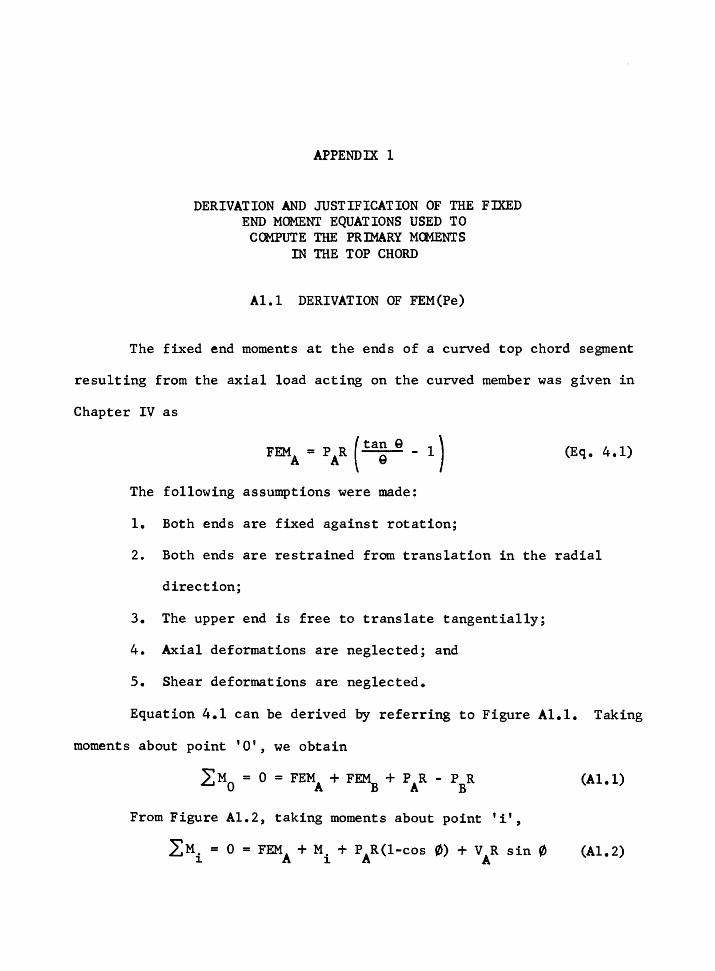
APPENDIX 1
DERIVATION AND JUSTIFICATION OF THE FIXED END MOMENT EQUATIONS USED TO
COMPUTE THE PRIMARY MCMENTS IN THE TOP CHORD
Al.l DERIVATION OF FEM{Pe)
The fixed end moments at the ends of a curved top chord segment
resulting from the axial load acting on the curved member was given in
Chapter IV as
FEM = P R ( tan Q - 1 ) A A Q
(Eq. 4.1)
The following assumptions were made:
1. Both ends are fixed against rotation;
2. Both ends are restrained from translation in the radial
direction;
3. The upper end is free to translate tangentially;
4. Axial deformations are neglected; and
5. Shear deformations are neglected.
Equation 4.1 can be derived by referring to Figure Al.l. Taking
moments about point 'O', we obtain
2:M0
= o = FEMA + FEM + P R - P R (Al. l) B A B
From Figure Al.2, taking moments about point 'i',
LM. = 0 = FEMA + M. + PAR(l-cos 0) + V R sin 0 i i A (Al. 2)
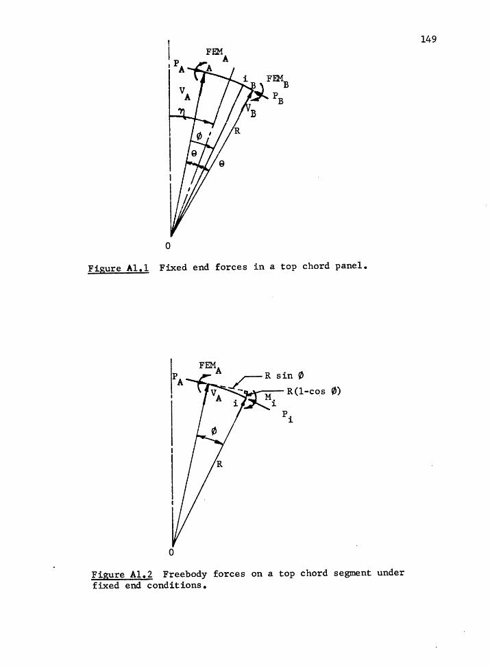
0
Figure Al.l Fixed end forces in a top chord panel.
0)
0
Figure Al.2 Freebody forces on a top chord segment under fixed end conditions.
149

or
Rearranging, we obtain
Swmning moments about point 'B' on Figure Al.1,
_L:~ = 0 = FEMA + F~ + PAR(l-cos 2~) +VAR sin 2Q
[
FEMA + F~ PA(l-cos 2Q)J VA = - R sin 2Q + --.;;;_s i-· n_2_Q __
150
{Al .3)
(Al.4)
Substituting Equation Al.4 into Equation Al.3, we obtain
[
FEMA + FEMBJ PA(l-cos 2Q) M. = -FEMA - PAR(l-cos 0) + . 29 (sin 0) + . 29 R sin 0
i sin sin {Al.S)
In order for the change in slope of the member at point 'A' to
be equal to zero (fixed),
For a constant EI,
12Q
0
~ d0 = 0 EI
Inserting Equation Al.S into Equation Al.6, we have
(Al.6)
12Q 2Q
FEMA O = -FEMA d0 + sin 29 (
o Jo 12Q
FEM sin 0<10 + sinB29 0 sin 0d0
p R (29
cos 0<10 + s~n 29(1-cos 29)}
0
sin 0d0 (Al. 7)

151
By observation of synmetry, it can be seen that
FEMA = -FE~
Therefore,
29 29 29 29
_ ( p A.R ) = -PAR(0) +PAR sin 0 sin 29 (1-cos 29)cos ~
0 0 0 0
which becomes
or
FEM = -P R + P R (sin 29) + p R {sin 29 ) ( 1-cos 29) 2
A A A 29 A 29 sin 29 {Al.8)
Further reduction yields
FEMA = PAR (-1 + si~929 + si~929(tan29))
=PAR (si~929(tan29+1) -1)
a PAR [ ( 2 sin 2~ cos 9 )( co>Q) -1 J or
FEM = P R ( tan 9 - 1 ) A A 9
(Eq. 4.1)
which is the desired result.
Al.2 JUSTIFICATION OF THE EXTERNAL LOAD INDUCED FEM's
In order to handle the case of the external member loads (which
may be unsymmetrical), we must satisfy the following three equations:

152
f B ~ = $ cos 9 EI I
A (Al. 9)
r B MxdX =-b sin g EI I
A (Al.10)
(Al.11)
The notation and tabular format used by Roark and Young in
their book Formulas for Stress and Strain, fifth edition(9) will be
used to organize the complex equations involved and to allow unusual
loading conditions to be considered. A few variables will be rede-
fined as noted below in order to facilitate the special case being
considered here.
The case being considered is described by reference number 13 of
Table 18 in Roark and Young.
Referring to Figure Al.3, the normal force at point 'A' has been
defined as VA and the tangential force as PA. The angle ~ , as defined
by Roark and Young, will be equal to -9 in this case. Thus, the equa-
tions given in Table 18, item 13 of Roark and Young become
SI(E:~c))= VA (BHV(c) + BHH(s)) + BHM (:A) - LFH (Al.12)
(Al.13)
(Al .14)

Figure Al.3 Model and nomenclature used by Roark and Young.
153

where
s = sin Q
c = cos e
E = Modulus of Elasticity
I = Moment of Inertia
R = Radius of Arch
B = Q + 29c2
- 3sc RH
2 B - B = 2s - 2Qsc RV - VH
BHM = BMH = 2s - 29c
2 B = Q + 29s - SC w B = B = 29s
VM MV
B = 29 MM
154
LFH, LFV and LFM are load factors which are defined for specific
load cases in Roark and Young, Table 18, ref. Sa through Sn.
also let,
1)
2)
2 Bl = BHV(c) + BHH(s) = Qs - s c
B2
= BW(c) + BVH(s) = Qc - sc2
+ 2s3
B3 = BMV(c) + BMH(s) = 2s2
a'= ( :n (c)
b' = ( :n (s)
We can therefore write,
( BVM) M = LF R A V
(Al. lS)
(Al.16)

155
3) (Al.17)
After performing Gaussian elimination on this set of equations,
we obtain
M = A
which can be rewritten as,
M = A
(LFH LFv)
a! + b'
further manipulation yields,
(Al.18)
(Al.19)
Defining the denominator as Q2
, we have, after algebraic manip
ulation,
Q2 = 2s2
- ( ~ ) 2
+ 9 ( ~ - 2sc) (Al. 20)
Also, defining
(Al. 21)
We thus have
(Al. 22)

156
Similarly, we can write,
_ LFM -B~(t) VA - B
3 {Al. 23)
and
~ = _l [cv )B + B (MA) - LF J I b A 2 VM R V (Al.24)
Letting
Q5
= (L _ 1 _ ~) 2s 2 2s
3
and
we then obtain,
R3 ~ LFV (MA)~ = - (Q )LF + - + Q -I EI 5 M s 6 R (Al. 25)
Now, knowing MA and VA' and assuming PA= O, we can obtain an
equation for~ by sunnning moments about point 'B'.
Thus,
~ = -M -[LFM - ~ MAJ R sin 29 + _L(Moments of external loads A B3 ~about point 'B') (Al.26)
which reduces to
Letting
( R sin 29) ~
2s2 LFM +~(MB of external loads)
'.J (Al. 27)
Q3
= 9 si~ 29 _1 s
29 tan 9 -1 and

we can then write,
R sin 2Q Q4 = 2s2 =
R tan Q
~ • [ Q3MA - Q4 (LFM) +~~of loads)]
157
(Al. 28)
Since we are dealing with elastic deformations, we add loadings
by the theory of superposition.
We therefore have, in summary,
(Al. 29)
(Al.30)
(Al.31)
where,
s = sin Q
c = cos Q
R = Radius of the Chord
1 (g 3 ) Q = - ~ + cs - c /s 1 2 2
s
Q2
= 2s2
- (9/s)2 + 9(c/s - 2sc)
Q3 2Q
1 = tan e
Q4 = R/tan g
2 ec Qs
c =-2 -1 --
2s 2s3

158
LFH, LFV and LFM are load factors obtained from Table 18, cases
Sa through Sn of Roark and Young, Fornru.las for Stress and Strain,
5th edition.
Now, consider a specific case in order to demonstrate that Equa-
tions Al.29 and Al.30 give the same answers as simply assuming the num-
ber to be a straight sloped beam, with the 'Pe' moment given from Eq.
4.1.
Al.2.1 Example Problem
The member shown in Fig. Al.4 is subject to a uniform vertical
load of 1 Kip per foot.
Since Table 18 of Roark and Young does not cover the specific
case loading shown, we must obtain the answers by superposition of
load cases Sd, Se and Sf.
Case Sd is a concentrated tangential load applied at an angle 0
from the center axis. In our case, 0=0, therefore, the equations for.
LFH,LFV and LFM as stated in Roark and Young become,
_ sc2
_ s _ c2
s ) 2 2
2 - 2s - SC ) (Al.32)
similarly,
2 2 LFVl = PA(c - 3s9 + (3/2)c(s -c) + c/2) =
2 PA (3) (cs -s9} (Al.33)
and
(Al.34)
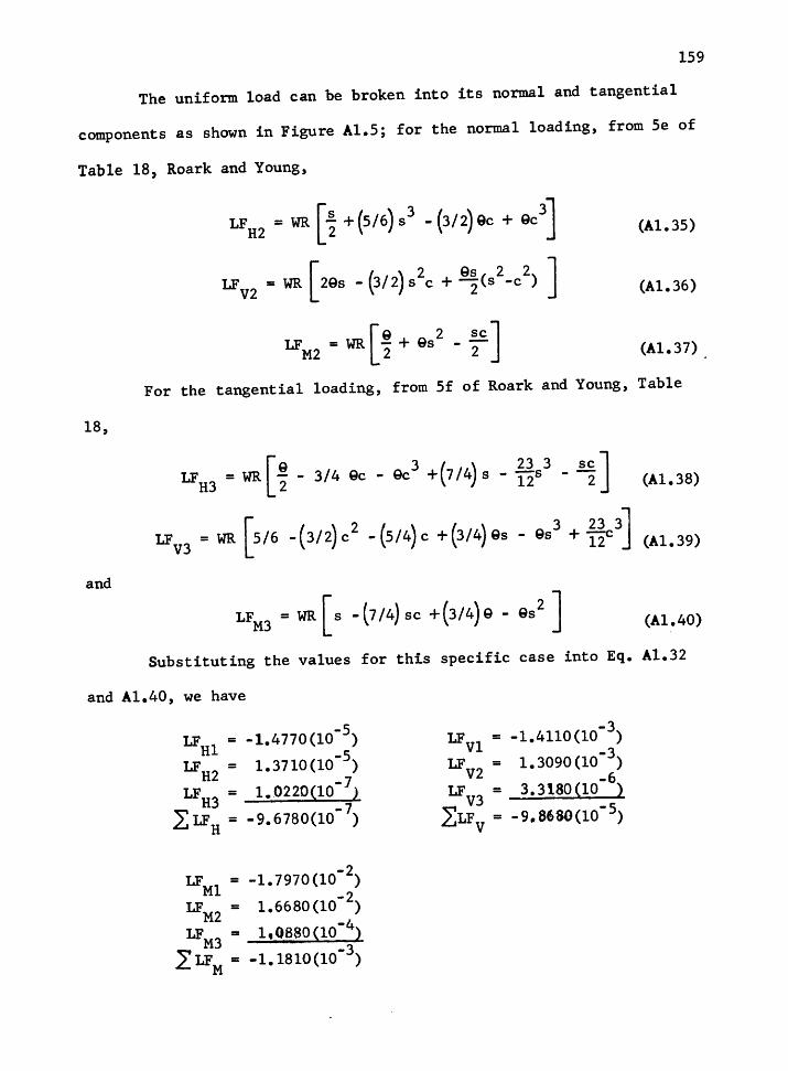
1S9
The uniform load can be broken into its normal and tangential
components as shown in Figure Al.S; for the normal loading, from Se of
Table 18, Roark and Young,
(Al.3S)
[ ( ) 2 Qs 2 2 J LFV
2 = WR 2Qs - 3/2 s c + ~(s -c ) (Al.36)
[Q 2 SC]
LFM2 = WR Z + Qs - 2 (Al.37)
For the tangential loading, from Sf of Roark and Young, Table
18,
[Q 3 ( ) 23 3 SC J LF = WR - - 3 / 4 Qc - Qc + 7 I 4 s - -s - -H3 2 12 2 (Al.38)
and
LFM3 = WR [ s -(7 /4) sc +(3/4) 9 - 9s2 J (Al.40)
Substituting the values for this specific case into Eq. Al.32
and Al.40, we have
LFHl = -1.4770(10-S) -s
LFH2 = 1.3710(10 ) -7
LFH3 = 1.0220(10 ) ~ -7 L..LFH = -9.6780(10 )
-2 LFMl = -1.7970(10 )
-2 LFM2 = 1.6680(10 )
LFM3
= 1,0880(10-4)
L LFM = -1.1810(10-3)
LFVl = -1.4110(10-3
) -3
LFV2
= 1.3090(10 )
LFV3
= 3.3180(10-6)
,L:LFV = -9-8680(10-S)
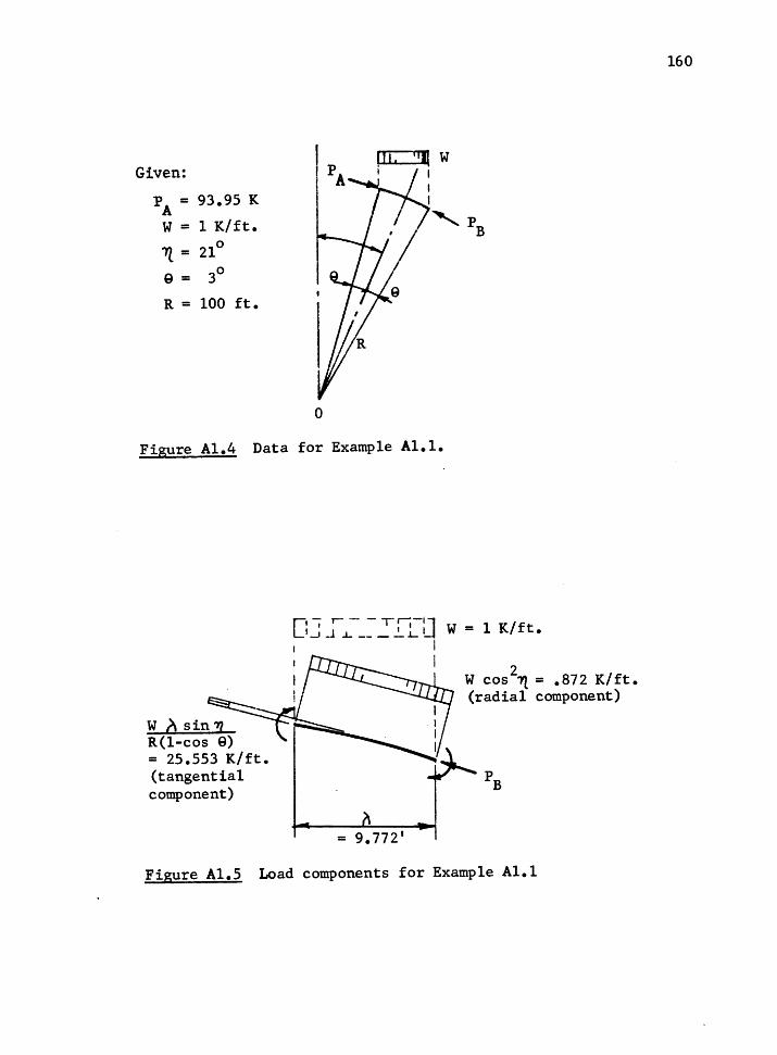
Given:
PA = 93.95 K
W = 1 K/ft.
7l = 210
9 = 3°
R = 100 ft.
0
Figure Al.4 Data for Example Al.l.
W o sin!l. R(l-cos 9) = 25.553 K/ft. (tangential component)
[I--; I - - 11.-11 1.....J -1 .L ___ _i_ l._ LJ W = 1 K/ ft.
I I I
2 W cos 11, = .872 K/ft. (radial component)
= 9.772'
Figure Al.5 Load components for Example Al.1
160

now computing the Q factors,
Ql = 6.9724(10-2)
Q2 = -1.8234(10-3)
Q3 = 9.982(10-1)
Q4 = 1.908(103
)
Q = -1.3322 5
Q6 = 3.4887(10-2
)
161
substituting these values and the values of LF into Eq. Al.29 and Al.30,
we obtain the following moments:
For 'Pe' only,
FEM = 8.5904l-k A
1-k Ffil\ = -8.5998
For the uniform load only,
FEMA = -7.692
FEMB = 8 .. 032
Using Eq. 4.1 for the 'Pe' moment, we obtain
FEMA = 8.595ll-k
Ffil\ = -8.595ll-k
The fact that FEMA I -F~ when computed using the Roark and Young
method is attributed to round-off error resulting from the numerous ca~
culations required. The average value of these moments is
FEM = 8.5904 ; 8.5998 = 8•5951 average

162
which is precisely the value obtained using the simplified method of
Eq. 4.1. Thus Eq. 4.1 appears valid for the assumptions made.
Computing the fixed end moments for a beam using the standard
formula for straight, sloped beams gives,
W ~ 2 )2
F '' w(9.i;2 -- -7.9581-k FEMA = - ~ = - 12 = - - -
which is within 3% of the answer obtained using the Roark and Young
formulas. Thus, we conclude that the simplified method is sufficiently
accurate.
Actually, the fixed end moments for the member loads will not be
precisely of equal magnitude. The tangential component of the load
will produce an unbalanced condition. This can be considered negligi-
ble in the geometries used in bowstring trusses as can be seen by the
relative magnitude of the LF factors of case 3 versus 1 and 2. The
net influence on the total unity equation for the member will be on the
order of 0.1%.
The curvature was found to have a small effect on the carry over
factor (CO) used in the moment distribution. The CO was computed to be
.5061 for an eight panel truss rather than the .50 which applies to a
straight beam. This is not considered to be of enough significance to
be considered and will be neglected. It should also be noted that the
chord is unrestrained against axial deformations and thus fixed end
axial forces do not affect the moments in the chord.

APPENDIX 2
SUMMARY OF THE FRAME ANALYSIS CCMPUTER DATA

164
TABLE A2.l
DATA FOR FIGURE 5.1
ABC IBC ATC ITC M M2 M M4 Designation NP 1 3
20TC11 100 250 75 800 8 1.23 0.23 o.o 02TC11 50 1800 75 800 8 10.94 2.92 o.o 12TC12 75 1800 75 1800 8 9.13 2.27 o.o 12TCOO 75 1800 so 2SO 8 12.88 2.26 o.o 12TC23 7S 1800 100 3600 8 7.36 2.23 o.o 33TC11 12S 3600 75 800 8 lS.67 3.37 o.o
20TC11 100 250 7S 800 10 1.Sl 0.19 0.45 o.o 02TC11 so 1800 75 800 10 12.91 2.93 4.31 o.o 12TC12 - 75 1800 75 1800 10 10.63 2.42 3.40 o.o 12TC20 7S 1800 100 250 10 9.39 1.94 3.09 o.o 12TC23 7S 1800 100 3600 10 8.30 2.so 2.92 o.o 33TC11 125 3600 75 800 10 17.79 4.00 5.30 o.o
31TC12 125 800 75 1800 12 4.96 0.91 1.06 1.09 03TC12 so 3600 7S 1800 12 2S.43 9.25 7.08 7.40 12TC12 75 1800 7S 1800 12 12.08 3.15 2.89 3.04 12TCOO 75 1800 so 250 12 17 .68 3.00 3.78 3.73 12TC32 7S 1800 12S 1800 12 8.78 2.68 2.30 2.48 33TC12 12S 3600 75 1800 12 19.25 S.71 4.50 4.74
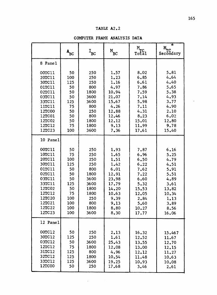
165
TABLE A2.2
COMPUTER FRAME ANALYSIS DATA
* ~c 1
Bc MBC MIC To al ~c Secondary
8 Panel
OOTCll 50 2SO 1.57 8.02 5.81 20TC11 100 250 1.23 6.85 4.64 30TC11 125 250 1.16 6.61 4.40 OlTCll so 800 4.97 7 .86 5.65 02TC11 50 1800 10.94 7.59 5.38 03TC11 50 3600 21.07 7.14 4.93 33TC11 125 3600 lS.67 5.98 3. 77 llTCll 7S 800 4.26 7 .11 4.90 12TCOO so 250 12.88 4.31 2.10 12TC01 so 800 12.46 8.23 6.02 12TC02 50 1800 12.12 lS.01 12.80 12TC12 7S 1800 9.13 11.99 9.78 12TC23 100 3600 7.36 17 .61 15.40
10 Panel
OOTCll so 250 1.93 7.87 6.16 lOTCll 7S 2SO 1.65 6.96 S.25 20TC11 100 2SO 1.Sl 6.50 4.79 30TC11 12S 250 1.42 6.22 4.Sl OlTCll so 800 6.01 7.62 S.91 02TC11 so 1800 12.91 7.22 S.Sl 03TC11 so 3600 23.98 6.60 4.89 33TC11 12S 3600 17.79 5.32 3.61 12TC02 so 1800 14.20 1S.S3 13.82 12TC12 7S 1800 10.63 12.05 10.34 12TC20 100 250 9.39 2.84 1.13 12TC21 100 800 9.13 S.60 3.89 12TC22 100 1800 8.80 10.27 8.56 12TC23 100 3600 8.30 17.77 16.06
12 Panel
OOTC12 so 2SO 2.13 16.32 15.467 30TC12 12S 2SO 1.61 12.s2 11.67 03TC12 so 3600 2S.43 13.55 12.70 12TC12 75 1800 12.08 13.00 12.15 31TC12 125 800 4.96 12.12 11.27 32TC12 125 1800 10.54 11.48 10.63 33TC12 12S 3600 19.2S 10.93 10.08 12TCOO so 250 17 .68 3.46 2.61

TABLE A2.2 continued
* ~c IBC ~c T~~l ~c Secondary
12TC03 50 3600 14.68 29.31 28.46 12TC11 75 800 12.74 6.75 5.90 12TC12 75 1800 12.08 13.00 12.15 12TC30 125 250 9.55 2.48 1.63 12TC31 125 800 9.22 5.25 4.40 12TC32 125 1800 8.78 9.82 8.97 12TC33 125 3600 8.14 16.92 16.07
* ~C(Secondary) = ~C(Total) - ~C(Primary) where
M.rc(Primary) (found from Figures 4.5, 4.7 and 4.9)
for each truss is as follows:
8 Panel -- ~C(Primary) = 2.21 Ft-K
10 Panel
12 Panel " "
= 1. 71 Ft-K
= 0.85 Ft-K
166

Primary Location Moment
J23 o.oo J25 J26 1.01 J27 J28 -1.09 J31 J32 -0.10 J33 J34 -0.32 J37 J38 -0.11 J39 J40 2.21 J41 J42 -2.95 J43 J44 o.oo
TABLE A2.3a
COMPUTER FRAME ANALYSIS DATA * USED TO PLOT FIGURE 6.la
8 PANEL TRUSS
12TC12 12TC23 Tot Mom Sec Mom Tot Mom
o.oo o.oo o.oo 1.80 2.37 2. 73 1. 72 3.87 2. 77 4.46 2.10 3.19 4.34 2.53 4.74 2.44 2.54 4.61 1.96 4.07 1.32 1.64 3.34 3.68 6.61 5.90 6.01 9.67 8.25 12.82
11.19 8.98 16.50 6.13 10.20 2.27 5.22 5.04 0.06 1.47 o.oo o.oo o.oo
*Data from Model III, Full Truss
167
Sec Mom
o.oo
2.86
5.43
4.71
3.66
9.78
14.29
7.99
o.oo

Location
Jl J2 J3 J4 JS JlO Jll Jl2 Jl3 Jl6 Jl7 Jl8 J19 J22 J23 J24 J25 J28 J29 J30 J31 J33 J34 J35 J36
Primary
TABLE A2.3b
CCMPUTER FRAME ANALYSIS DATA USED TO PLOT FIGURE 6.lb
12 PANEL TRUSS
12TC12 Moment Tot Mom Sec Mom
o.oo o.oo o.oo 0.35 1.09 0.74 0.37 1.81 1.44 0.08 2.25 2.17
-0.50 2.35 2.85 -0.06 2.69 2.75 0.10 2. 72 2.62 0.02 2.48 2.46
-0.25 2.05 2.30 -0.04 2.46 2.50 0.04 2.75 2.71 0.05 2.91 2.86 0.06 3.15 3.09
-0.15 3.01 3.16 -0.28 2.87 3.14 -0.22 2.96 3.18 0.09 3.30 3.21
-0.06 5.38 5.46 -0.05 7.64 7.69 0.21 10.17 9.96 0.85 13.00 12.15
-0.43 8.75 9.18 -1.09 5.06 6.15 -0.99 2.08 3.07 o.oo o.oo o.oo
168
12TC33 Tot Mom Sec Mom
o.oo o.oo 1.52 1.17 2.66 2.29 3.52 3.46 4.03 4.53 4.36 4.42 4.37 4.27 4.11 4.09 3.65 3.90 4.07 4.11 4.37 4.33 4.54 4.49 4.78 4. 72 5.02 5.17 5.24 5.52 5.69 5.91 6.35 6.26 8.65 8.71
11.12 11.17 13.87 13.66 16.92 16.07 11.69 12.12 7.01 8.10 3.05 4.04 o.oo o.oo

APPENDIX 3
"PINNED MEMBER" DESIGN METHOD
The classical method of considering secondary stresses in
trusses consists of computing the joint deflections based on a pin
jointed truss analysis. These deflections are then used as support
settlements for the continuous chord which allows the moments to be
computed. This method is only approximate, but is reasonably accurate
for most design work. It should be noted that the deflection perpen
dicular to the top chord should be used when computing top chord mo-
ments.
The slight error in this method stems from the fact that the
secondary moments cause some redistribution of axial forces in the mem
bers which will affect deflections. In bowstring trusses, an addition
al error is introduced by the fact curved top chord changes length not
only due to the axial stress deformation, but also as a result of the
bending moments ( SI' derived in appendix 1).
The & I value for primary moments is generally small compared to
the axial deformation. However, as was shown, the secondary moments
may be much larger than the primary moments. These moments will be
positive moments (tending to decrease curvature) and as a result will
tend to lengthen the member.
The redistribution of forces in the end two webs is also signi
ficant which tends to smooth the deflected shape.

170
These two factors result in deflections computed assuming
straight pinned end members being greater than will actually occur.
Thus, the secondary moments computed by this technique will be conser
vative. In most cases, however they will represent the actual stress
es accurately enough for design purposes.
Joint slippage can be introduced in this method in any of the
conventional ways, normally by including a fixed internal deflection
component into the virtual work sunn.nation process, or if a matrix ana
lysis is used,- the member areas can be artificially modified to affect
a larger member deformation.

APPENDIX 4
''GENERAL CHARACTERISTIC EQUATION'' METHOD COMPUTER PROGRAMS

PROGRAM I. DATA BASE PREPARATION
10 PRINT "NUMBER OF PARAMETERS" 20 INPUT N 30 OPEN 11 0°,•t, 11 COUNTER.DAT" 50 PRINT •t,N 60 DIM X<N,3> 70 DIM XNAMESCN> 80 FOR 1•1 TO N 90 PRINT "X<";I;">NAME ?" 100 INPUT XNAMES<I> 110 NEXT I 120 PRINT 11 NUMBER OF VARIABLES?" 130 INPUT M 150 PRINHH, M 170 DIM YNAMESCM> 180 FOR I=l TO M 190 PRINT 11 YC";I;">NAME?" 200 INPUT YNAMES<I> 210 NEXT I 220 PRINT "ENTER BASE VALUES" 230 FOR 1=1 TO N 240 PRINT XNAMESCl>; 11 2=" 250 INPUT X<I,2> 260 NEXT I 270 PRINT "ENTER THE OTHER VALUES FOR EACH PARAMETER" 280 FOR Icl TO N 290 PRINT XNAMES<I>;"1=" 300 INPUT X<I,1> 310 PRINT XNAMES<I>;"3=" 320 INPUT X<I,3> 330 NEXT I 340 INPUT "NO. OF LOAD CASES";NL 360 PRINT#1,NL 370 CLOSE #1 380 REM 390 REM DETERMINE ALL REQUIRED COMPUTER RUNS 400 REM 410 PRINT 420 PRINT "COMPUTER RUNS REQUIRED" 430 PRINT 440 PRINT "BASE VALUES: 450 FOR I=l TO N 460 PRINT XNAMES<I>;"="IX<I,2> 470 NEXT I 480 PRINT 490 PRINT 50'21 PRINT ," RUN","ALL BASE VALUES" 5UJ PRINT , " NUMBER 11
, "EXCEPT LET:"
172

520 PRINT "------------------------------------" 530 PRINT , " BASE" 540 FOR 1=1 TO N 550 PRINT , XNAME4*<I>;"1",XNAME4*<1>;"=";X<I,1>, 560 FOR LD=l TO NL 570 PRINT "LD"i <LD>, 580 NEXT LD590 PRINT 600 PRINT , XNAME4*<I>;"3",XNAME4*<I>;"=";X<I,3>, 610 FOR LD=l TO NL 620 PRINT "LD";LD, 630 NEXT LO 640 PRINT 650 NEXT I 660 PRINT 670 PRINT 680 PRINT "MODEL THE STRUCTURE AND COMPLETE COMPUTER" 690 PRINT 11 RUNS FOR EACH OF THE ABOVE CASES" 700 PRINT 710 OF·EN 11 0 11
, 4t2, "PARAMETR. DAT" 720 FOR I=l TO N 730 FOR CASE=1 TO 3 740 PRINT4t2,X<I,CASE> 750 NEXT CASE 760 NEXT I 790 FOR Iz1 TO N 800 PRINT4t2,XNAME4*<I> 810 NEXT I 840 FOR J=1 TO M 850 PRINT4t2,YNAME4*<J> 860 NEXT J 880 PRINT "EXECUTION COMPLETE" 885 END
173

PROGRAM II. DEVELOPMEl'n OF CHARACTERISTIC EQUATIONS
09121 r;~M TH l S f.·POGF:.~M DE'.'E:UJF'ES THE CONSTANT FOR THE 081 REM CHARACTERISTIC EQUATIONS 985 Ii'JF'UT "F'RINfER CONNECTED (1 ORY: YES>":F'F:• 89\!J OF'EN II I ... • 1 • II COUNTER. DAT II
•7,~H~t INPUT # 1 • N 9~tZJ I NF'UT it 1 , M q4~J I NF'UT tH. ML 95!!1 OF'EN II I 11 '#:2. "F'AF'AMETR. DAT" 970 FOR I= 1 TO N 975 FOR CASE =1 ro 3 98L";f ItlPUT #2. X ( ! . C.:ASE >
1 ~1~>1z1 NE X T CASE 1~H 5 NEXT I 10~0 FOR 1=1 TO N 1030 INPUT #2~XNAME$CI> 1•!14!2t NEXT I 1060 FOR J=l TO M 1070 INPUT #:~YNAME$(J) Hl8(3 NEXT J 1090 DIM BCN.M~NL> 1100 DIM G<N,M.NL> 1110 DIM k<N.M.NL> 1120 DIM C<N,M.NL) 1130 DIM YB<M.NL> 1135 DlM YCN.2.M,NL> 1140 DIM TY<M.NL> 1 1 5 ~!J D I M T 0 TY .: M ) 11 6 et D I M T X < N > 11 7 ~!J 0 p EN II 0 II ' # 3 ' II E QUA T I ON • DAT II 1180 FOR LO= 1 TO NL 1200 FOR J=1 TO M 1 2 UZJ pp I NT y NAME$ ( J ) ; II <BA SE !' II ~ L D; II ) =? "
174
1220 INPUT YBCJ.LO> 123~3 PRINT#3, YB CJ, LD>: IF F'R$= 11 l '' OR PR$="Y" THEN LF'F:INT
YNAME$ ( J) ; " <BASE. II ; LD; II ) =" ; YB ( J 'LO) 124~!J NEXT J 1241 NEXT LD 1243 FOR L0=1 TO NL 1245 FOR I=l TO N 1247 FOR CASE =1 TO 2 1249 FOR J=l TO M 1251 F'F:INT YNAME$<J>; II~"; XNAME$(!) ;CASE; 11 L0 11 :LD=
11
)?"
1253 INPUT Y<l.CASE~J.LD> 1254 IF F'F:S="l" OR PR!="Y" THEN LF'RINT il'JAMES(J):" ( 11 ; XNAMES (I>: CASE: "LO"; LO">=": Y <I, CASE. J ~LO' 1255 NEXT J 1257 tJEXT CASE
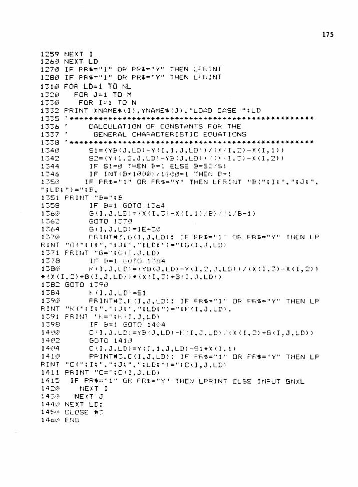
1259 NEXT I 12fr~I NEXT LD 127iZI IF PR$= II 1 II OR F'R$= II y II THEN LF'F: I NT 1 :Sf2J I F F'F\'$ = II 1 II OR p F: $ = II y II THEN L F'R I NT
131g FOR LD=i TO NL 13:?!21 133Ql 13.32 13:.5 1336 1337 1338 134l2l 134:2 1344 1 :A6 1 :::5i2!
FOR J=l TO M FOR 1=1 TO N
FRINT XNAME$<l).YNAME$(J)."LOAD CASE ";LD ~****************•**•••***~•···*••••****************
CALCULATION OF CONSTANTS FOR THE GENERAL CHARACTERISTIC EQUATIONS
~*********•4••*·~··*•••****•***4*•••·••************* Sl= ~YB (J .. LD) -Y (I. 1. J. LD:1 > / ( X: I. :2) -X (I !I 1) > S:?=<Y<I.:? •. J~LD~-YBi:J.LD) >...-('a' I~ 3)-X <1.2)) IF 51=0 THEN B=l ELSE B=S~'Sl IF I NT i. El• 11~l·JQ!) I l •?\•J1Z!= 1 THEN I>= 1
I F F' R $ = II 1 II 0 R F' F: $ = " y II THEN L F F: I NT " B ( II ~ I ; II .. " : J ' II "
";LD; ")=":B. 1351 1:.ss 136QI 1362 1364 1 :.:~~j F:INT 1 .:.: . . ! 1 1378
F'F:INT "B=": B I F E<= 1 GOT 0 1 36 4 G ( I , \.1 • LD > = ( X < I • 3;. - X ( I • 1 :i / B:. / 1
' l / B-1 >
GOTO 137.:Z! G(l,.J.LD)=1E+30 F' f;• ItH # 3 • G ( I • J • L D ) : I F F' F' $ = II 1 '. 0 F: F' F: $ = II y II THE l'J L p
II G ( II ' I ; II ' II : J; II .. ,, ; LD; II ) =II' G ( I • ,J • LD)
F'Rlt·ff "G="; G (I. J. LO> IF B= 1 G1JTO 1 ::;94
1 3 8 ~25 V ( I • J .. L [• 1 = ( Y B \ J • L D ) - Y ( I • 2 • ,J • L [i ) ) I ( X ( I ~ 3 ) - X ( I , 2 > )
* ( X < I , ~ > +G < ! .. J .. Lr•.' ) • ( >: <I" 3 > +G ( I .. \.1. LD) i 1 38'.2 GOTO 1 :;9~~1 1384 ~:i'.l.J.LD·=Sl
13·1~2j F'R I nT#3. ~,· ·'.I. J. LD > : IF PF:$-= 11 1 " OR F'F:$= .. v 11 THEN LP F: I NT II v ( " : I ; II • II ; .:,T ~ II •
11 : L D : II ) = " : ~. ( I • J • L [\ ) •
1 ::._91 FRir.Jl 1• k= '';I<; I. J ~ L.D>
1398 IF 8=1 GOTO 1404 14 1 ~1~2!
14!~12
14(14 1410 F:INT 1411 1415 14:s?I
c: I • J. L[1' =YB I J" LD) -~:: i, I" J. LD) / 1'. x (I. 2) +G (I~ J. LD) }
GOTO 14 L~! C<I.J.LD>=Y<J.1.J .. LD>-Sl•X<J.1) F'F:INT .. 3.C<I,J.LD>: rr= F'R$="1" OR F'P$="Y" THEN LP
II c ( t:; I ; II. ti: J: II" "; LD' 01 ) = 11
: c ( I "J. LD) F'RINT "C='': C' I. J. LD>
IF F'R$==" 1" OF: F'Rt= 11 Y~ 1 THDJ LPF:INT ELSE Ir-Jr:·UT GNXL t-JEXT I
! 4 :.i'.I NE ·r:T J 1 4 4 :J NE X T L D : 145•.~> CL.CSE ~-:,
l •lc!~1 Et>JD
175

PR<X;RAM III. DESIGN PROCEDURE
2~:,~!l!!l OF'EN II 1 " ... 3 .. "EOUAT ION. OAT11
~(~'1'~' ,_:PEN II I II c tt2. 11 F'AhA~1ETF:. DAT" :2 i~' ·.: \!J Cl F' EN " I I' • " 1 ' II c 0 u NT ER . DAT II 2~!1-~)~I I NFUT 1t 1 , N 2!!'4~~1 !r-lF'U T tt 1 • M
176
2~~15!-~1 i r-JF'UT 1+ 1. NL ::051 DlM GCN.M.NL).K<N.M,NLl4CtN.M~NL).Y8CM,NL>.TY<M~NL 1 .T OTYCM>,TXCN>.XNAME$CN>,YNAME$CM> 2052 FOR I=l TO N 2053 FOR CASE= 1 TO 3 2054 INPUT #2.~0THING ::055 NEXT CASE '.2 ~~! 5 6 NE X T I ::>J6•-:I FCJR I= 1 TO N 2070 INPUT #2.XNAME$(l) :2!'.18;~t NE)( T I 2090 FOR J=1 TO M 2100 INPUT #2.YNAME$(J) 2 1 l 1ZJ NE "'. T J ~1:0 DIM PLD <NL> 2130 FOR LD=l TO NL 2140 FOR J=l TO M 2150 INPUT #3,YB(J,LD> 21Ml NEXT J 21 7~21 t-JE ~: T LD 2180 FOR LD=l TO NL 2190 FOR J=1 TO M 2200 FOR I=l TO N 2210 INPUT #3,G(l,J.LD> 2220 INPUT #3,k(I,J,LO):INPUT #3.C<I,J,LD> 223QJ NEXT I 224!!1 NEXT J 225~:~) ~.:E :1~ T LO 2260 REM DESIGN SECTION 2265 DL$= 11 Y11
2270 FOR I= 1 TO N 2 2 8<.ZI F' ~: I MT II T F: ! AL II ; x NAME$ ( I ) ; II = II ;
229!~; I NF'UT T 2292 IF T=0 THEN 2300 2294 T"/.(I>=T 2:.i!\~~J t·JE :X T I 2"3i~i5 r F OL $=" 1 " OF: OL $=" Y" THEN GOTO 23 u~j ELSE GOTO 2:::4121 2310 FOR LD=l TO NL 2 3 1 5 p R I NT II~~ LOAD c A SE I I = L D ;
2320 INPUT PLDCLO> 233•:!1 tJEXT LO 2340 FOR J=1 TO M

238~1
2:.92 2::.9\!t
177
rorv < J > =\!t FOR LO= 1 TO NL TY<J.LD>=Y0\J.LD> <1-N)
FOR I=l TO N IF G <I. J. LO> =1E+"31~ THEN GOTO ~:,94 TY< J. LO> =TY~ J, LO> • ( t- <I. J. LO> I <TX < I> +G < I.
J. LO> > +C \ I , J. LO> > 2::92 2394
GOTO 24\~h!' TY<J,LD>=fY(J.LD>•<K'l.J,LD>*TX<I>•C<I~J
, LO>; 24 i~l\3 24!~S5
241 ~3 242(.!f
NEXT I TY<J.LD>=TY<J.LD>•PLD<LD> F'RINf YNAMES~J): '' <LD":LD~ ")=": TY<J~LD' TOTY\J>=TOTY<J>+TY<J,LD>
24 3<~ NEXT LO 2 4 4(!'5 F' F: I NT y NAME$ \ J ) ; " = II ; T 0 Ty ( J ) : .. T 0 T AL II
2451!t t·JE X T J 246~3 INPUT II CHANGE F'AF:AMETEF:S II; QCS 2465 I NF'UT ''CHANGE LOAD I NG'': QL·S 247!~• IF lJS="Y" OR Q$= "YES" OR Q$=" 1" THEN GOTO 227~3 2490 FOR I= 1 TO N 25·'.1(3 LPF:INT XNAMES (I);"=": TX\ I>.
2510 NEXT I 2515 LF'F:INT 2520 FOR LD=l TO NL 25-:Q• LF'F: I NT "I. LOAD CASE II: LD: ti= •. : F'LD ( LD) '
2540 NEXT LD 2545 LF'F: I NT 2550 FOR J=l TO M 256i2f LPR I NT 't'NAME$ ( J) ; II=,, ; TOTY ( J)
257\!J NEXT J 2575 INPL!T "CHANGE FAF:AMETERS":; OS 2576 IF 0$="Y" OR Q$= 11 YES 11 OR Q$="1" THEN GOTO 2270
258l~ END

REFERENCES
1. Laursen, H.I. 1969. Structural Analysis, McGraw-Hill Book Company.
2. The American Institute of Timber Construction, 1974. Timber Construction Manual, Second Edition, John Wiley and Sons, Inc.
3. Mueller, W.H. III. RIGID, A Frame and Truss Analysis Program, Civil-Structural Engineering, Portland State University.
4. Bathe, K.J., Wilson, E.L., and Peterson, F.E. SAP IV, A Structural Analysis Program for Static and Dynamic Response of Linear Systems, June 1973, Revised April 1974, College of Engineering, University of California, Berkeley, California.
s. The American Institute of Timber Construction. AITC 117-79-Design Standard Specifications for Structural Glued Laminated Timber of Softwood Species, Adopted as Recommendations June 27, 1979.
6. GTICES Systems Laboratory. GTSTRUDL, School of Civil Engineering, Georgia Institute of Technology, Atlanta, Georgia.
7. National Forest Products Association. National Design Specification for Wood Construction, 1982 Edition, National Forest Products Association, WashingtQn, D.C.
8. Bradford, J.F. Timber Design - 1982 NDS, Dick w. Ebeling, Inc., Portland, Oregon.
9. Roark, R.J. and Young, w.c. 1975. Formulas for Stress and Strain, Fifth Edition, McGraw Hill Book Company.