Second Welfare Theorem

Econ 2100 Fall 2015

Lecture 18, November 2

Outline

1 Second Welfare Theorem

From Last Class

We want to state a prove a theorem that says that any Pareto optimalallocation is (part of) a competitive equilibrium.

That will entail finding the prices that make that allocation an equilibrium.

First, we had to change the definition of equilibrium to deal with budgetconstraints.

Given an economy({Xi ,%i , ωi}Ii=1 , {Yj}

Jj=1

), an allocation x∗, y∗ and a price

vector p∗ are a price equilibrium with transfers if there exists a vector ofwealth levels

w ∈ RL withI∑i=1

wi = p∗ ·I∑i=1

ωi +J∑j=1

p∗ · y∗j

such that:1. For each j = 1, ..., J: p∗ · yj ≤ p∗ · y∗j for all yj ∈ Yj ;2. For each i = 1, ..., I : x∗i %i xi for all xi ∈ {xi ∈ Xi : p∗ · xi ≤ wi} ;

3.I∑i=1x∗i ≤

I∑i=1ωi +

J∑j=1y∗j , with pl = 0 if the inequlity is strict for good l .

Need Interior Allocations

Picture

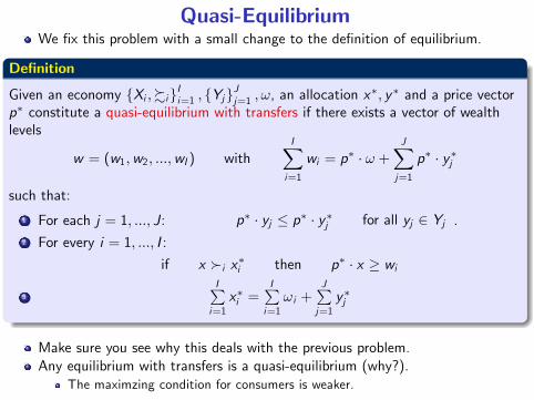
Quasi-EquilibriumWe fix this problem with a small change to the definition of equilibrium.

Definition

Given an economy {Xi ,%i}Ii=1 , {Yj}Jj=1 , ω, an allocation x

∗, y∗ and a price vectorp∗ constitute a quasi-equilibrium with transfers if there exists a vector of wealthlevels

w = (w1,w2, ...,wI ) withI∑i=1

wi = p∗ · ω +J∑j=1

p∗ · y∗j

such that:

1 For each j = 1, ..., J: p∗ · yj ≤ p∗ · y∗j for all yj ∈ Yj .2 For every i = 1, ..., I :

if x �i x∗i then p∗ · x ≥ wi

3

I∑i=1x∗i =

I∑i=1ωi +

J∑j=1y∗j

Make sure you see why this deals with the previous problem.Any equilibrium with transfers is a quasi-equilibrium (why?).

The maximzing condition for consumers is weaker.

Second Welfare Theorem: Preliminaries

We have seen a few counterexamples to a possible second welfare theorem.

This is what we need to avoid those issues.

To show that for any Pareto optimal allocation one can find prices thatmake it into a competitive equilibrium requires a few assumptions

We need to transfers to overcome the limitations imposed by privateownership.

We need convexity of production sets.

We need convexity and local non-satiation of preferences.

We need to eliminate boundary issues.

Second Welfare Theorem

Theorem (Second Fundamental Theorem of Welfare Economics)

Consider an economy({Xi ,%i}Ii=1 , {Yj}

Jj=1 , ω

)and assume that Yj is convex for

all j = 1, ..., J, and %i is convex and locally non-satiated for all i = 1, ..., I .

Then, for each Pareto optimal allocation x , y there exists a price vector p 6= 0 suchthat (x , y , p) form a quasi-equilibrium with transfers.

The proof uses the separating hyperplane theorem.

If an allocation is Pareto optimal there is an hyperplane that simultaneouslysupports the better-than sets of all consumers and all producers.That hyperplane yields a candidate equilibrium price vector.

The proof is in three parts: aggregation, separation, and decentralization.

We start with a Pareto optimal allocation and construct the correspondingquasi-equilibrium with transfers.

Proof of the Second Welfare Theorem: Aggregation

First, we aggregate all consumers preferences when evaluating the Paretoeffi cient consumption bundle x∗.

Define the following sets:

Vi = {xi ∈ Xi : xi � xi} ⊂ RL and V =∑i

Vi

V is the set of all bundles strictly preferred to x by every consumer.

Claim: V is convex.

Take x ′,x ′′ ∈ Vi (so both are strictly preferred to xi ) and w.l.o.g. assumex ′ %i x ′′.Since preferences are convex, for any λ ∈ [0, 1]

λx ′ + (1 − λ) x ′′ %i x ′′By transitivity, we have

λx ′ + (1 − λ) x ′′ %i x ′′ �i xiTherefore, λx ′ + (1 − λ) x ′′ is an element of Vi and therefore each Vi is convex.V is convex because it is the sum of I convex sets.

Proof of the Second Welfare Theorem: Aggregation

Second, we aggregate all firms and define the set of attainable consumptionbundles.

Define the aggregate production set as

Y =∑j

Yj =

∑j

yj ∈ RL : y1 ∈ Y1, ..., yJ ∈ YJ

The set of consumption bundles that can be allocated to consumers is

Y + {ω}This set is convex since it is the sum of J + 1 convex sets.

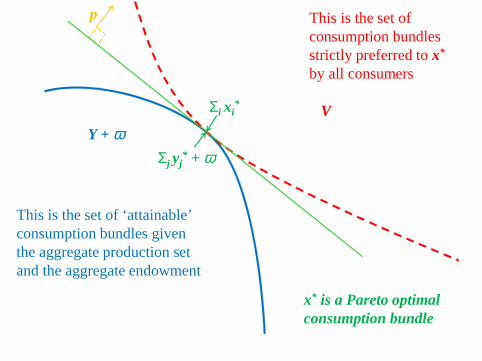
Geometry of the Proof

Draw V and Y + {ω}.

V=ΣiVi = Σi {xi in Xi : xi>xi*}

Y + ω

This is the set ofconsumption bundlesstrictly preferred to x*

by all consumers

This is the set of ‘attainable’consumption bundles giventhe aggregate production setand the aggregate endowment

x* is a Pareto optimalconsumption bundle

Σi xi*

Proof of the Second Welfare Theorem: Separation

Next, we separate the sets V and Y + {ω}.

Since (x , y) is a Pareto optimal allocation, V ∩ Y + {ω} = ∅.If not, some consumer can obtain a consumption bundle preferred to what shegets in x , contradicting the assumption that x is Pareto optimal.

Since V and Y + {ω} and two disjoint convex sets, one can apply theSeparating Hyperplane Theorem.

Separate V and Y + {ω}By the Separating Hyperplane Theorem, there exist a p ∈ RL with p 6= 0 and anr ∈ R such that

p · z ≥ r for all z ∈ V ,and

p · z ≤ r for all z ∈ Y + {ω}

Proof of the Second Welfare Theorem: SeparationNext, we look at the implication of separation for consumers. By separation,

p · z ≥ r for all z ∈ V ,

Claim: if xi %i xi for all i , then p · (∑

i xi ) ≥ rremember this aswe will use it later

Take any xi %i xi for all i .By local non-satiation, for each i there exists an xi (near xi ) such that xi �i xi .Hence, xi ∈ Vi for all i , and

∑i xi ∈ V .

So, p · (∑

i xi ) ≥ r (by separation);Take a sequence of xi that goes to xi (check how this works): p · (

∑i xi ) ≥ r .

Applying this result to xi %i xi , separation tells us that

p ·(∑

i

xi

)≥ r

Geometry of the Proof

We have shown that∑

i {xi ∈ Xi : xi %i xi} belongs to the closure of V whichis contained in the half-space

{z ∈ RL : p · z ≥ r

}.

VY + ω

This is the set ofconsumption bundlesstrictly preferred to x*

by all consumers

This is the set of ‘attainable’consumption bundles giventhe aggregate production setand the aggregate endowment

x* is a Pareto optimalconsumption bundle

Σi xi*

p

Proof of the Second Welfare Theorem: SeparationNext, use the implication of separation for firms. By separation

p · z ≤ r for all z ∈ Y + {ω}

Choosing z =∑

j yj + ω ∈ Y + {ω} one getsp · (

∑j

yj + ω) ≤ r

Next, put together the implications of separation for consumers and firms.The Pareto optimal allocation is feasible, and therefore:∑

i

xi ≤∑j

yj + ω ∈ Y + {ω}

Hence we havep ·(∑

i

xi

)≤ r

Putting together this inequality and the opposite one from the previous slide:

p ·(∑

i

xi

)= r

Geometry of the Proof∑i xi belongs to Y + {ω} and it lies in the half-space

{z ∈ RL : p · z ≤ r

}.

VY + ω

This is the set ofconsumption bundlesstrictly preferred to x*

by all consumers

This is the set of ‘attainable’consumption bundles giventhe aggregate production setand the aggregate endowment

x* is a Pareto optimalconsumption bundle

Σi xi*

Σj yj* + ω

p

Second Welfare Theorem Proof: DecentralizationWe have shown the following holds

p ·(∑

i

xi

)= p ·

ω +∑j

yj

= r

Claim: x satisfies the consumers’condition in a quasi-equilibrium with transfers atprices p = p.

For some consumer i , take an x such that x �i xi . We need to show thatp · x ≥ wi for some wi .As shown previously,

p∗ ·

x +∑n 6=ixn

︸ ︷︷ ︸

this satisfies xi%i xi for all i

≥ r = p∗ ·

xi +∑n 6=ixn

Hence:p · x ≥ p · xi

Set wi = p · xi so that we have p · x ≥ wi as desired.

Second Welfare Theorem Proof: DecentralizationWe have shown the following holds

p ·(∑

i

xi

)= p ·

ω +∑j

yj

= r

Claim: y maximizes profits at prices p.

For any firm j and any yj ∈ Yj , we haveyj +

∑k 6=j

yk ∈ Y

Hence, by separation and the equation above we have

p ·

ω + yj +∑k 6=j

yk

≤ r = p ·

ω + yj +∑k 6=j

yk

Hence,

p · yj ≤ p · yjTherefore, yj maximizes profits at prices p.

Proof of the Second Welfare Theorem: End

SummaryWe have shown that x satisfies the consumers’condition in a quasi-equilibriumwith transfers at prices p and income wi = p · xi .We have also shown that yj maximizes profits at prices p.

Therefore

We have shown that the Pareto optimal allocation (x , yj ) and the prices p form aquasi-equilibrium with transfers.

The equilibirum prices are given by an hyperplane that simultaneously supportsall consumers better-than set and the aggregate production set.

Proof of the Second Welfare Theorem: Coda

The last step is to show that a quasi-equilibrium with transfers is also anequilibrium with transfers.

You will prove this in Problem Set 9.

First, you have to show that, under local non satiation, if there is a consumptionbundle cheaper than a consumer’s wealth, condition 2. of a quasi-equilibriumwith transfers is equivalent to condition 2. of an equilibrium with transfers(there is nothing strictly cheaper than ωi in our counterexample from last class).Then, add strict monotonicity (something else violated by that counterexample)and show that a quasi equilibrium with transfers which has strictly positivewealth for all consumers is an equilibrium with transfers.

What Are The Welfare Theorems About?

The first welfare theorem says a competitive equilibrium is Pareto effi cient:markets can yield effi cient allocations.

The second welfare theorem says that any Pareto effi cient allocation can beobtained as an equilibrium provided one makes the ’right’adjustment toincome.

In other words, any outcome that maximizes social welfare can be obtained byredistributing income ’correctly’across consumers.

There are many caveats to these results

Both theorems rule out externalities.Both theorems need local non satiation.For the second welfare theorem, even assuming all assumptions are satisfied, weneed someone to decide what are the transfers.

This is not practical as this someone would need to know everyone’s preferences,and all production sets, to figure those transfers out. How do you know those?In public economics, and optimal taxation theory, one asks if there is a way toget the consumers to reveal their preferences to the planner.

Next Week

Equilibrium characterization in the differentiable case.

Welfare theorems in the differentiable case.

Existence.

Welfare Theorems in the Differentiable Case

QuestionWhat is the relationship between the first order conditions that correspond to acompetitive equilibrium and those that give Pareto optimality?

Assumptions needed for differentiabilityConsumers

Let Xi = RL+ and assume there exist ui (x) representing %i that satisfy strongmonotonicity and convexity for each i .Normalize things so that ui (0) = 0.Assume each ui (x) is twice continuously differentiable, with ∇ui (x)� 0 forany x , and also assume that ui (x) is quasi-concave.

Producers

Production sets are Yj ={y ∈ RL : Fj (y ) ≤ 0

}, where Fj (y ) = 0 defines the

transformation frontier.Assume each Fj (y ) is convex, twice continuously differentiable, with∇Fj (y )� 0 for any y , and also assume that Fj (0) ≤ 0.

Welfare Theorems in the Differentiable Case

Given these assumptions, Pareto effi ciency solves the planners problem.

RemarkAn allocation is Pareto optimal if and only if it is a solution to the following:

max(x ,y )∈RLI×RLJ

u1 (x11, x21, ..., xL1)

subject to

ui (x1i , x2i , ..., xLi ) ≥ ui i = 2, 3, ..., I

∑i

xli ≤ ωl +∑j

ylj l = 1, 2, ..., L

Fj (y1j , ..., yLj ) ≤ 0 j = 1, 2, ..., J

Welfare and Equilibirum In the Differentiable Case

(x∗, y∗) is Pareto optimal if and only if it solves the following

max(x ,y )∈RL(I+J)

u1 (x1) s.t.ui (xi ) ≥ ui i = 2, 3, ..., IFj (yj ) ≤ 0 j = 1, 2, ..., J∑

i xli ≤ ωl +∑

j ylj l = 1, 2, ..., L

We can also write the maximization problems that must be solved by acompetitive equilibrium.

(x∗, y∗, p∗) is a competitive equilibrium with transfers if x∗, y∗ solves:

maxxi≥0

ui (xi ) s.t. p∗ · xi ≤ wi i = 2, 3, ..., I

andmaxyjp∗ · yj s.t. Fj (yj ) ≤ 0 j = 1, 2, ..., J

What is the connection between the first order conditions of these twooptimization problems?