second order analysis in braced slender … · a slender column is defined as a column that is...
TRANSCRIPT
118
Journal of Engineering Sciences
Assiut University
Faculty of Engineering
Vol. 45
No. 2
March 2017
PP. 118 – 141
SECOND – ORDER ANALYSIS IN BRACED SLENDER COLUMNS
PART I: APPROXIMATE EQUATION FOR COMPUTING THE
ADDITIONAL MOMENTS OF SLENDER COLUMNS
M. A. Farouk
Civil engineering Department, Engineering collage, Al - Jouf University
Received 10 January 2017; Accepted 15 February 2017
ABSTRACT
Second- order analysis in braced slender columns was investigated in this study. The present study
is concerned with two main points. The first point is focusing on how to compute the additional
moments in slender columns according to accredited equations in different codes as well as the basics
and the assumptions of these equations. In the second point, approximate equation was suggested to
compute the additional moments in slender columns. This equation was proved in elastic analysis and
for the cases of single curvature in slender columns. The equation was proved by considering the
column supported on two pin supports with rotational springs. The rotational springs represent the
connected beams with the columns. The suggested equation gave matching values of the induced
additional moments of slender columns compared with finite element results in elastic analysis.
Keywords: Second order; Finite element; Additional moment; Slender column.
1. Introduction
A slender column is defined as a column that is subjected to additional moments due to
lateral deflections. These moments cause a pronounced reduction in axial-load capacity of
the column. In first-order analysis, the effect of the deformations on the internal forces in
the members is neglected. In second-order analysis, the deformed shape of the structure is
considered in the equations of equilibrium. However, because many engineering
calculations and computer programs are based on first-order analyses, methods have been
derived to modify the results of first-order analysis to approximate the second-order
effects. Second order analysis in slender columns is recommended in many codes by using
approximate equations to compute the additional moments. The additional moments in
slender columns according to accredited equations in different codes, as well as the basics
and the assumptions of these equations will be discussed in next section.
2. Calculation of the additional bending moments ( addM ) in slender
columns according to different codes
The Egyptian Code]1[ takes into consideration increasing the applied moments in
slender columns by adding an additional moment to the original moment. The secondary
119
M. A. Farouk, second – Order analysis in braced slender columns Part 1: approximate …….
moments are assumed to be induced due to interaction of the axial load with the lateral
deformation of the column.
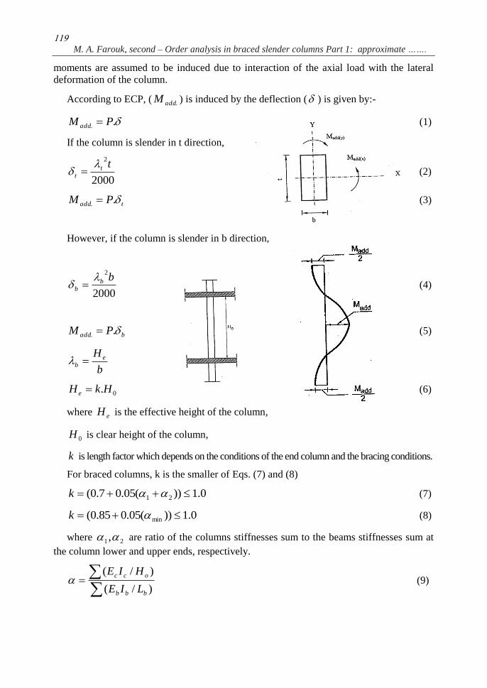
According to ECP, ( .addM ) is induced by the deflection ( ) is given by:-
.. PM add (1)
If the column is slender in t direction,
2000
2tt
t
(2)
tadd PM .. (3)
However, if the column is slender in b direction,
2000
2bb
b
(4)
badd PM .. (5)
b
H e
b
0.HkH e (6)
where eH is the effective height of the column,
0H is clear height of the column,
k is length factor which depends on the conditions of the end column and the bracing conditions.
For braced columns, k is the smaller of Eqs. (7) and (8)
0.1))(05.07.0( 21 k (7)
0.1))(05.085.0( min k (8)
where 21, are ratio of the columns stiffnesses sum to the beams stiffnesses sum at
the column lower and upper ends, respectively.
)/(
)/(
bbb
occ
LIE
HIE (9)
120
JES, Assiut University, Faculty of Engineering, Vol. 45, No. 2, March 2017, pp.118–141
In fact, ECP doesn't mention the basis of equation (5), or the presuppositions which the
equation was based on.
The British Code ]2[ uses the same equation of ECP for the computation of addM in slender
column. Prab Bhatt et al ]3[ illustrated the basis and the assumptions of the British code as follows:
Additional moment is a function of the columns lateral displacement. The code aims to
predict the deflection at mid-height at the moment of concrete failure.
The shape of the curvature is assumed, and the central deflection
ua is assumed to be given by,
2.e
u lEI
aPa
u (10)
EI
aP
r
u.1 (11)
where r
1 is the curvature. The curvature will vary typically along the column and the code
assumes a sinusoidal value of2
1
. Thus the central lateral deflection ua is assumed to be:
rla eu
11 2
2 (12)
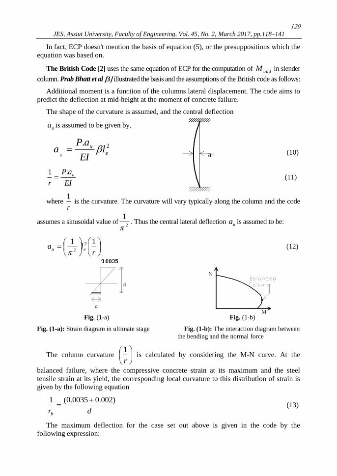
Fig. (1-a) Fig. (1-b)
Fig. (1-a): Strain diagram in ultimate stage Fig. (1-b): The interaction diagram between
the bending and the normal force
The column curvature
r
1 is calculated by considering the M-N curve. At the
balanced failure, where the compressive concrete strain at its maximum and the steel
tensile strain at its yield, the corresponding local curvature to this distribution of strain is
given by the following equation
drb
)002.00035.0(1 (13)
The maximum deflection for the case set out above is given in the code by the
following expression:
121
M. A. Farouk, second – Order analysis in braced slender columns Part 1: approximate …….
h
la e
u
20005.0 (14)
hh
lha e
u .2000
).(2000
22 (15)
Where: el and h are effective buckling height of column and column thickness, respectively.
Some important notes can be observed from basics of the used equations in the British
and Egyptian codes,
In these equations, the deflection shape is assumed as sine curve, even if the
columns are subjected to end moments.
These equations are valid only in the ultimate stage. This means that these
equations are not valid in working stress design or at any stage before the ultimate.
The equations take into account the connected beams rigidity in the calculation of the
column effective length without considering the effect of these beams in the reversal
moments, which can be induced at the connection between them and the columns.
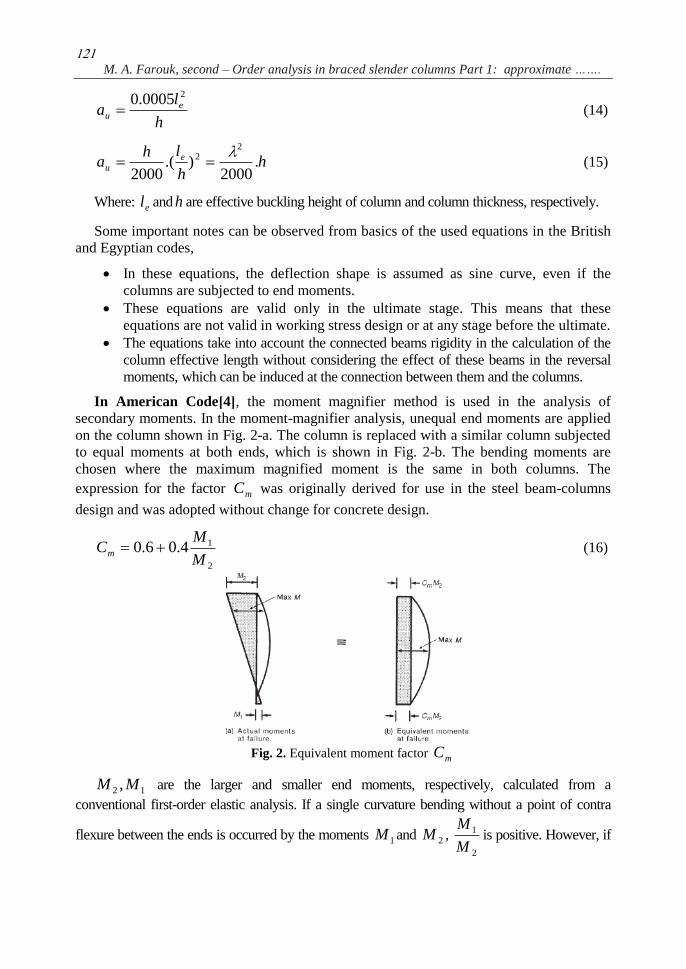
In American Code]4[, the moment magnifier method is used in the analysis of
secondary moments. In the moment-magnifier analysis, unequal end moments are applied
on the column shown in Fig. 2-a. The column is replaced with a similar column subjected
to equal moments at both ends, which is shown in Fig. 2-b. The bending moments are
chosen where the maximum magnified moment is the same in both columns. The
expression for the factor mC was originally derived for use in the steel beam-columns
design and was adopted without change for concrete design.
2
14.06.0M
MCm (16)
Fig. 2. Equivalent moment factor mC
12 , MM are the larger and smaller end moments, respectively, calculated from a
conventional first-order elastic analysis. If a single curvature bending without a point of contra
flexure between the ends is occurred by the moments 1M and 2M , 2
1
M
Mis positive. However, if
122
JES, Assiut University, Faculty of Engineering, Vol. 45, No. 2, March 2017, pp.118–141
the moments cause double curvature with a point of zero moment between the two ends, that
2
1
M
Mis negative. The moment magnifier equation in the cases of no sway according to ACI is,
2.MM nsc (17)
The subscript ns refers to no sway. The moment 2M is defined as the greater end
moment acting on the column. ACI Code goes on to define ns as follows:
c
mns
P
P
C
75.01
(18)
The 0.75 factor in Eq. (18) is the stiffness reduction factor ϕK, which is based on the
probability of under strength of a single isolated slender column.
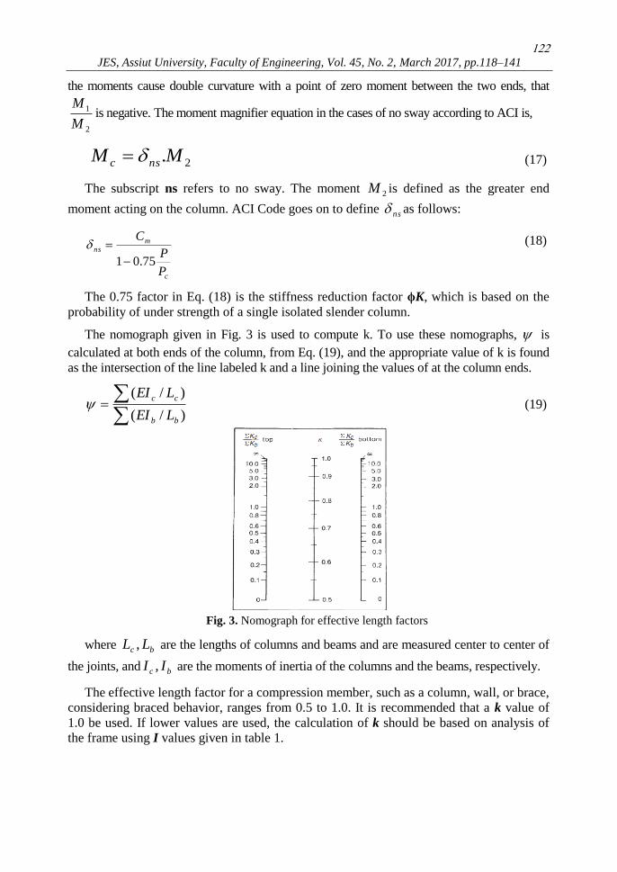
The nomograph given in Fig. 3 is used to compute k. To use these nomographs, is
calculated at both ends of the column, from Eq. (19), and the appropriate value of k is found
as the intersection of the line labeled k and a line joining the values of at the column ends.
)/(
)/(
bb
cc
LEI
LEI (19)
Fig. 3. Nomograph for effective length factors
where bc LL , are the lengths of columns and beams and are measured center to center of
the joints, and bc II , are the moments of inertia of the columns and the beams, respectively.
The effective length factor for a compression member, such as a column, wall, or brace,
considering braced behavior, ranges from 0.5 to 1.0. It is recommended that a k value of
1.0 be used. If lower values are used, the calculation of k should be based on analysis of
the frame using I values given in table 1.
123
M. A. Farouk, second – Order analysis in braced slender columns Part 1: approximate …….
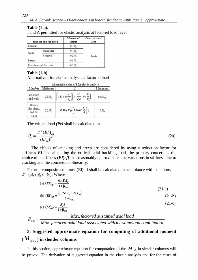
Table (1-a).
I and A permitted for elastic analysis at factored load level
Table (1-b).
Alternative I for elastic analysis at factored load
The critical load (Pc) shall be calculated as
2
2
)(
)(
u
eff
ckL
EIP
(20)
The effects of cracking and creep are considered by using a reduction factor for
stiffness EI. In calculating the critical axial buckling load, the primary concern is the
choice of a stiffness (EI)eff that reasonably approximates the variations in stiffness due to
cracking and the concrete nonlinearity.
For non-composite columns, (EI)eff shall be calculated in accordance with equations
21- (a), (b), or (c): Where
(21-a)
(21-b)
(21-c)
ncombinatioloadsamethewithassociatedloadaxialfactoredMax
loadaxialsustainedfactoredMaxdns
.
.
3. Suggested approximate equation for computing of additional moment
( addM ) in slender columns
In this section, approximate equation for computation of the addM in slender columns will
be proved. The derivation of suggested equation in the elastic analysis and for the cases of
124
JES, Assiut University, Faculty of Engineering, Vol. 45, No. 2, March 2017, pp.118–141
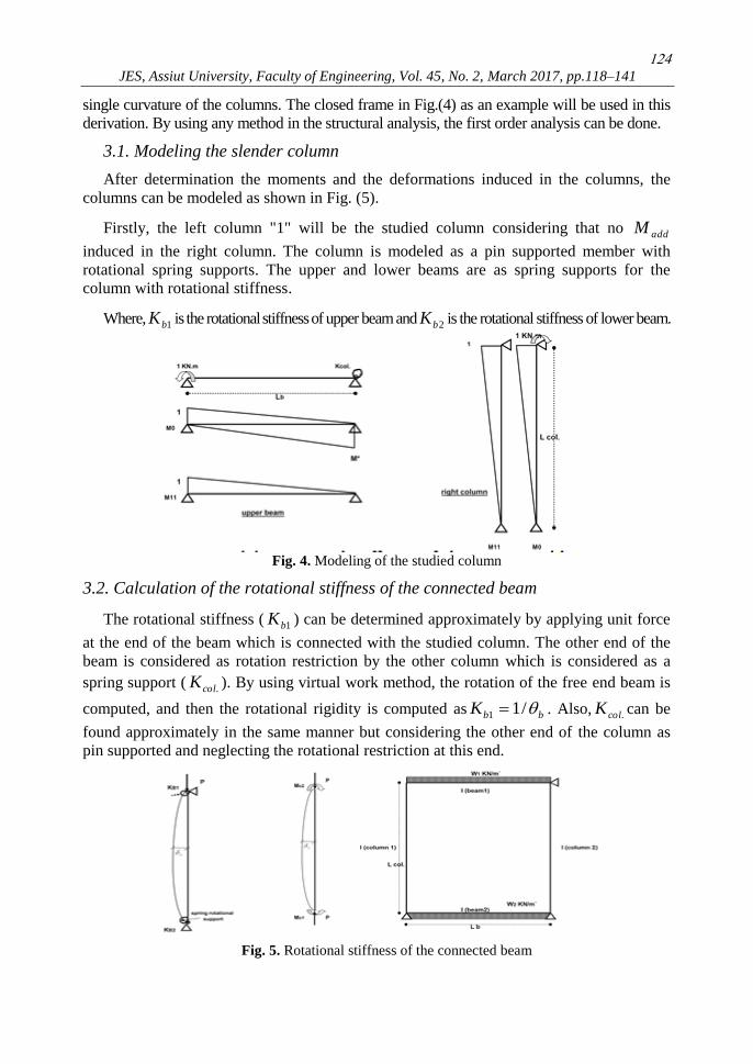
single curvature of the columns. The closed frame in Fig.(4) as an example will be used in this
derivation. By using any method in the structural analysis, the first order analysis can be done.
3.1. Modeling the slender column
After determination the moments and the deformations induced in the columns, the
columns can be modeled as shown in Fig. (5).
Firstly, the left column "1" will be the studied column considering that no addM
induced in the right column. The column is modeled as a pin supported member with
rotational spring supports. The upper and lower beams are as spring supports for the
column with rotational stiffness.
Where, 1bK is the rotational stiffness of upper beam and 2bK is the rotational stiffness of lower beam.
Fig. 4. Modeling of the studied column
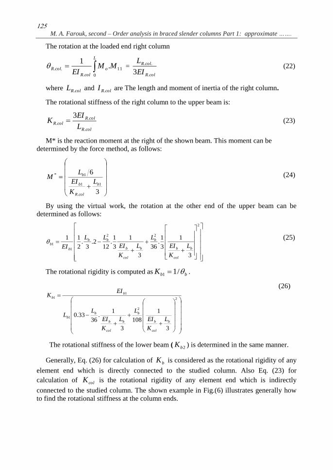
3.2. Calculation of the rotational stiffness of the connected beam
The rotational stiffness ( 1bK ) can be determined approximately by applying unit force
at the end of the beam which is connected with the studied column. The other end of the
beam is considered as rotation restriction by the other column which is considered as a
spring support ( .colK ). By using virtual work method, the rotation of the free end beam is
computed, and then the rotational rigidity is computed as bbK /11 . Also, .colK can be
found approximately in the same manner but considering the other end of the column as
pin supported and neglecting the rotational restriction at this end.
Fig. 5. Rotational stiffness of the connected beam
125
M. A. Farouk, second – Order analysis in braced slender columns Part 1: approximate …….
The rotation at the loaded end right column
L
o
colR
colR MMEI
0
11
.
.. .1
= colR
colR
EI
L
.
..
3 (22)
where colRL . and colRI . are The length and moment of inertia of the right column.
The rotational stiffness of the right column to the upper beam is:
colR
colR
colRL
EIK
.
.
.
3 (23)
M* is the reaction moment at the right of the shown beam. This moment can be
determined by the force method, as follows:
3
6
1
.
1
1*
b
colR
b
b
L
K
EI
LM (24)
By using the virtual work, the rotation at the other end of the upper beam can be
determined as follows:
2
22
1
1
3
1
3
1.
36
3
1
3
1.
122.
3.
2
11
b
col
b
b
b
col
b
bb
b
b L
K
EI
L
L
K
EI
LL
EI
(25)
The rotational rigidity is computed as bbK /11 .
2
2
1
1
1
3
1
108
3
1.
3633.0
b
col
b
b
b
col
b
b
b
b
b
L
K
EI
L
L
K
EI
LL
EIK
(26)
The rotational stiffness of the lower beam ( 2bK ) is determined in the same manner.
Generally, Eq. (26) for calculation of bK is considered as the rotational rigidity of any
element end which is directly connected to the studied column. Also Eq. (23) for
calculation of colK is the rotational rigidity of any element end which is indirectly
connected to the studied column. The shown example in Fig.(6) illustrates generally how
to find the rotational stiffness at the column ends.
126
JES, Assiut University, Faculty of Engineering, Vol. 45, No. 2, March 2017, pp.118–141
2
33
2
3
33
33
3
3
1
108
3
1.
3633.0
L
KK
EI
L
L
KK
EI
LL
EIK
CJCGCJCG
BC
2
55
2
5
55
55
5
3
1
108
3
1.
3633.0
L
K
EI
L
L
K
EI
LL
EIK
EFEF
BE
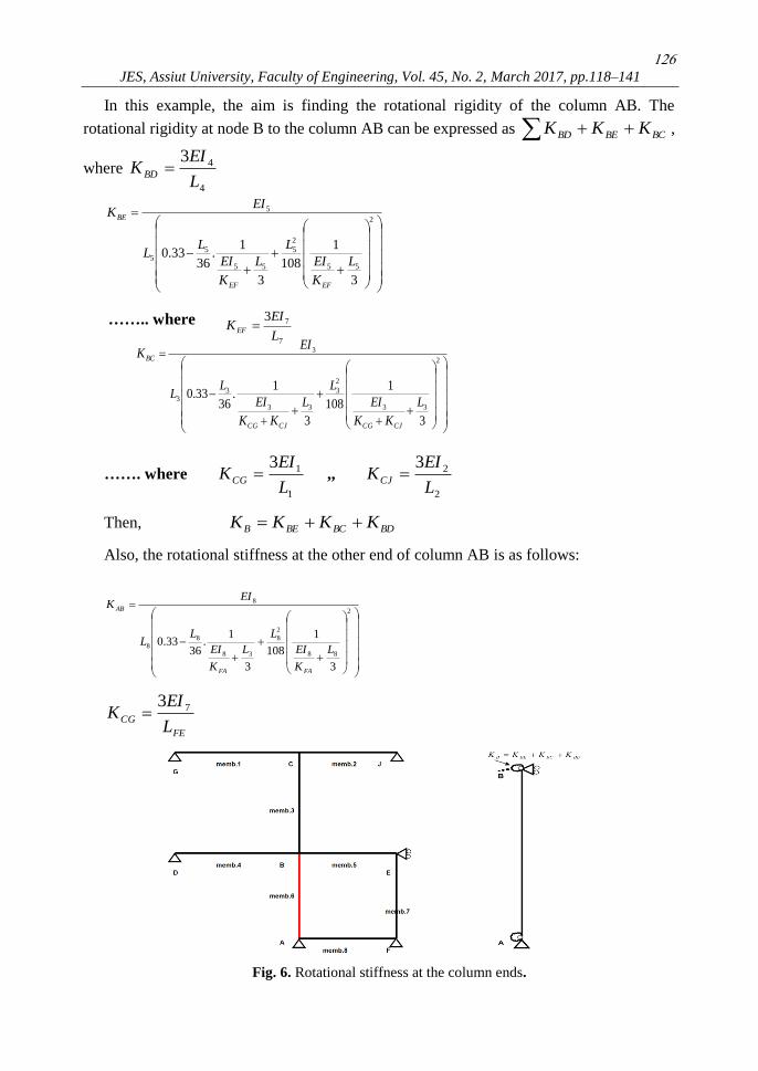
In this example, the aim is finding the rotational rigidity of the column AB. The
rotational rigidity at node B to the column AB can be expressed as BCBEBD KKK ,
where 4
43
L
EIK BD
…….. where
7
73
L
EIK EF
……. where
1
13
L
EIKCG ,,
2
23
L
EIKCJ
Then, BDBCBEB KKKK
Also, the rotational stiffness at the other end of column AB is as follows:
2
88
2
8
38
8
8
8
3
1
108
3
1.
3633.0
L
K
EI
L
L
K
EI
LL
EIK
FAFA
AB
FE
CGL
EIK 73
Fig. 6. Rotational stiffness at the column ends.
127
M. A. Farouk, second – Order analysis in braced slender columns Part 1: approximate …….
From many trials, it was found that, for any element that is connected to a column
whether it was another column or a beam, and has a cross section greater than or equal to the
studied column cross section, the rotational rigidity in Eq. (26) can be simplified to Eq.(23)
element
element
L
EIK
3
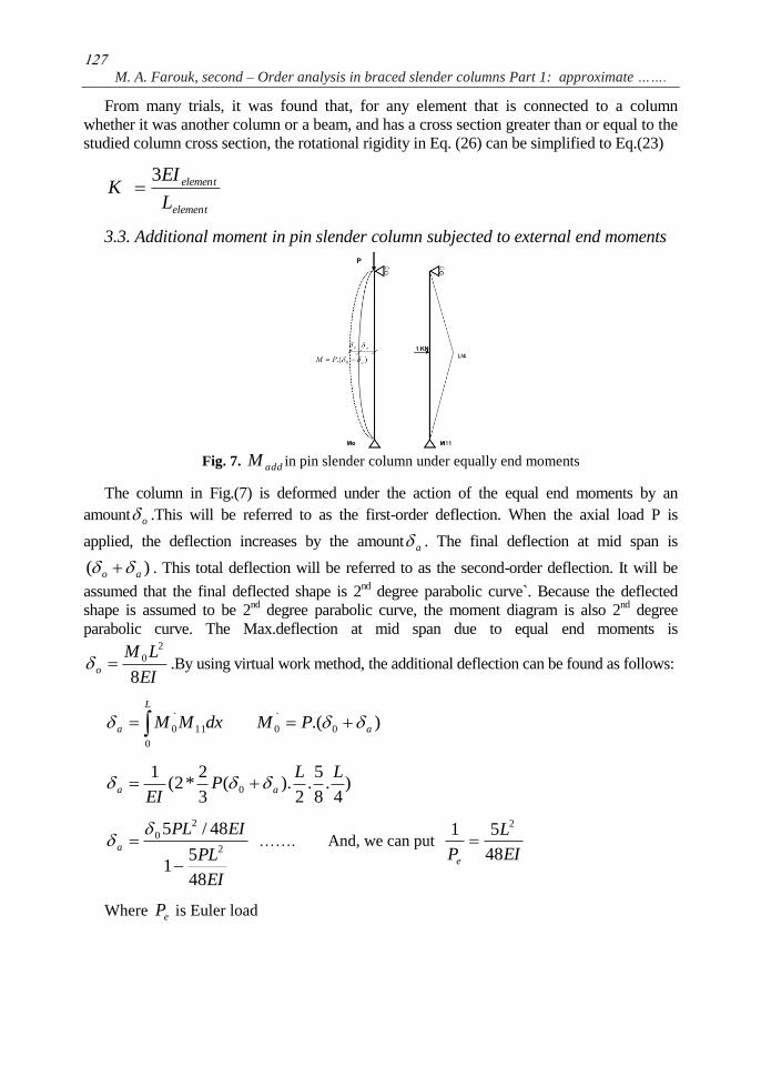
3.3. Additional moment in pin slender column subjected to external end moments
Fig. 7. addM in pin slender column under equally end moments
The column in Fig.(7) is deformed under the action of the equal end moments by an
amount o .This will be referred to as the first-order deflection. When the axial load P is
applied, the deflection increases by the amount a . The final deflection at mid span is
)( ao . This total deflection will be referred to as the second-order deflection. It will be
assumed that the final deflected shape is 2nd
degree parabolic curve`. Because the deflected
shape is assumed to be 2nd
degree parabolic curve, the moment diagram is also 2nd
degree
parabolic curve. The Max.deflection at mid span due to equal end moments is
EI
LMo
8
2
0 .By using virtual work method, the additional deflection can be found as follows:
L
a dxMM0
11
`
0 ).( 0
`
0 aPM
)4
.8
5.
2).(
3
2*2(
10
LLP
EIaa
EI
PL
EIPLa
48
51
48/52
2
0
……. And, we can put EI
L
Pe 48
51 2
Where eP is Euler load
128
JES, Assiut University, Faculty of Engineering, Vol. 45, No. 2, March 2017, pp.118–141
e
a
P
P
1
0 …… with putting
eP
P
1
1
Then, oadd PM … 2nd
parabolic curve (27)
Similarly, when the column is deformed under unequal end moments, the moments are
divided into two parts MMM 0 .The deflection curve of M is 3rd
degree
parabolic curve, and the maximum deflection occurs when 0dx
d. The maximum
deflection in this case is at 0.54L from the smaller moment. Thus Max. deflection due
to M is given by EI
ML
56.15
2`
0
.
Thus, the additional deflection is
e
a
P
P
94.01
`
0`
(28)
By rounding the term
eP
P
94.01
1
to , it is considered that the total additional
deflection in the case of unequal end moments is at distance equal to 0.54L from the
smaller moment, and is expressed as:
)( `
ooat (29)
So, when the column is deformed under unequal end moments, the maximum addM
through the middle of the span can be considered as:
)56.158
(22
0
.EI
ML
EI
LMPM add
(30)
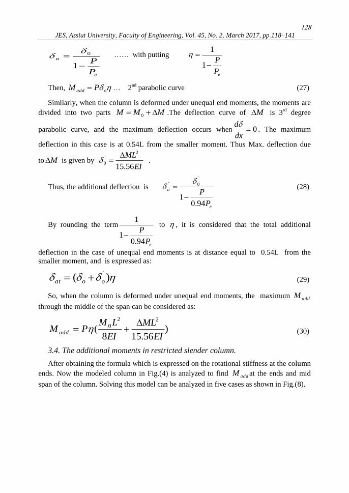
3.4. The additional moments in restricted slender column.
After obtaining the formula which is expressed on the rotational stiffness at the column
ends. Now the modeled column in Fig.(4) is analyzed to find addM at the ends and mid
span of the column. Solving this model can be analyzed in five cases as shown in Fig.(8).
129
M. A. Farouk, second – Order analysis in braced slender columns Part 1: approximate …….
Fig. 8. addM in restricted slender column
where:-
case 1:- )56.158
(22
0
.EI
ML
EI
LMPM add
:- addM at mid span
due to the axial force and the deflections from moments.
Case 2:- 1M is the induced moments at the spring support "1"
Case 3:- )( `
1 aP is addM at mid span due to the axial force and the deflections from 1M .
Case 4:- 12 MMM is the difference between the larger moments induced at
spring support "1" and the smaller moments induced at spring support "2".
Case 5:- )( `̀
2 aP is addM at mid span due to the axial force, the deflections
from M and its additional deflection.
Using the moment area method to solve these cases as follows:-
`
.
21 .. xEI
Ax
col
m
aba (31)
where mA is the area of moments between the nodes1,2.
3..
2
1
256.15*46.0*65.0
8.
2
1.
3
2
56.15*46.0*65.0
8*2.
3
2
..
2
.
1
2
.1
2
.1
2
.1
2
0
.
2
.0
.
2
.
.
1
.1
colcolcol
col
col
col
col
col
col
colcol
b
col
LM
LM
EI
LM
EI
LM
EI
LM
EI
LM
EI
LPL
K
EIM (32)
130
JES, Assiut University, Faculty of Engineering, Vol. 45, No. 2, March 2017, pp.118–141
3..
2
1
2)
56.15*46.0*65.0
8.
2
1.
3
2
56.15*46.0*65.0
8*2.
3
2(..
1.
.
2
.
1
2
.1
2
.1
2
.1
2
0
.
2
.02
.
.
1
1
colcolcol
col
col
col
col
col
col
col
b LM
LM
EI
LM
EI
LM
EI
LM
EI
LMLP
EIL
K
M
(33)
col
col
col
col
colcol
col
colcol
b
col
EI
MLLP
MLQLPLP
EI
LMM
L
K
LM 2
2
2
22
2
1
1
2
1
1 31.0
6.
242
(34)
By putting col
col
col
col
EI
LM
EI
LMQ
56.15315.0
24
2
0
2
0 (35)
col
colcol
col
colcol
b
colcolEI
LPLMQLP
EI
LPL
K
EILM
56.15
315.0
6(.
242
142
2
42
.
1
1
(36)
)242
(....2
.
2
1
..
1
col
colcol
b
colcol
EI
LL
K
EILZputting (37)
1
421
).100
94.16
(ZEI
LPLA colcol
(38)
MAQLPZ
M col
2
1
1 .1
(39)
.
21
col
m
EI
A
)56.15
65.083
2(
56.15.65.0
28.
3
2
)(.
2
0
2
0
.
3
.
3
.1
.1
1
.
2
.
1
2
.
EI
LM
EI
LMLP
EI
MLPML
EI
LMPLM
K
EI
K
EIM
K
EIM
col
col
col
colcol
col
col
col
b
col
b
col
b
col
(40)
)56.15
65.0
2()
12(
2
3
*
3
12
1
b
col
col
colcol
col
col
col
col
bb K
EI
EI
LPLMQLP
EI
LPL
K
EI
K
EIM
(41)
Where col
col
col
col
EI
LM
EI
LMQ
56.15656.0
8.
3
22
0
2
0* (42)
And putting
131
M. A. Farouk, second – Order analysis in braced slender columns Part 1: approximate …….
2
3
12 12)
11( Z
EI
LPL
KKEI
col
col
col
bb
col
(43)
)56.15
*67.05.0(2
8.
3
2
2
33
1
.
2
.
1
b
col
col
col
colcol
col
col
col
b
col
b
col
K
EI
EI
LPLMPQL
EI
LPL
K
EI
K
EIM
(44)
)
56.15
*67.05.0(2
1
2
3
2
1
b
col
col
col
colcolK
EI
EI
LPLMPQL
ZM
(45)
By solving equations 36 and 45
6100
201
1000
67.41
2
1
.22
1
2
3
2
1
2
2
*
col
col
col
b
col
col
colcol
col
L
EI
LP
Z
K
EI
EI
LPL
Z
Z
LQP
Z
LPQM
(46)
And putting
2
3
2 1000
67.41
2
1.
b
col
col
colcol
K
EI
EI
LPL
ZB
(47)
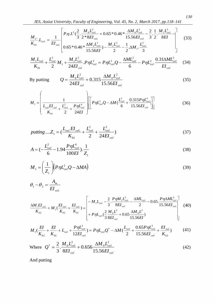
The additional moment can be obtained in the final formulas as follows:
MBZ
LPQM col
2
.
*
1
(48)
BAZ
QL
Z
QLPM col
col
1.
1
2
.
2
*
. (49)
MMM 12 (50)
Where 1M at the beam which has the smaller rigidity and 2M at the beam this has
higher rigidity. And the terms of equation 2
*
1 ,,,, ZQAZQ and B are shown in equations
(35, 37, 38, 42, 43 and 47), respectively.
MMPM momid 58.0).( 1
**
. (51)
Where
midM is the additional moments through the middle of column length.
*)56.158
(.
2
0
.
2
0*
0
col
col
col
col
EI
LM
EI
LM (52)
132
JES, Assiut University, Faculty of Engineering, Vol. 45, No. 2, March 2017, pp.118–141
*)56.158
(.
2
.
2
1*
col
col
col
col
mEI
ML
EI
LM (53)
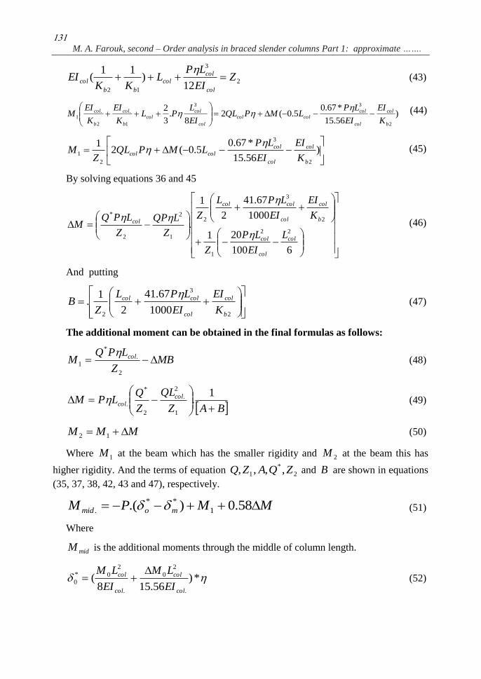
3.5 Effect of additional moment in the adjacent columns on the studied column
From the proved previous equations, additional moments at the ends and at mid span of
the column can be computed. These equations are proved hence there are no addM
considered in the adjacent columns.
To take into consideration the effect of addM of other columns on the studied column,
assuming in the example in Fig.(3) that the addM induced in the right column are
determined according to Eqs. (48 to 51). Also, as shown in Fig.(9), part of these moments
will transfer to the studied left column through the beams. By considering one of the ends of
these beams is subjected to addM which are coming from the ends of the right column, and
the other end of the beams is rotationally restrained by the studied left column as shown in
Fig.(9). The force method can be used to find the transferred moments to the studied column.
Fig. 9. The effect of addM in the adjacent columns
133
M. A. Farouk, second – Order analysis in braced slender columns Part 1: approximate …….
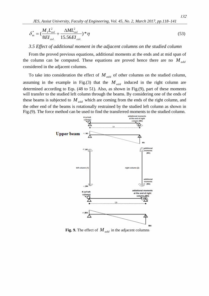
Fig. 10. The transferred moments to the lower end of column 1
For example to find the transferred moments to the bottom end of column 1,
colK
MM
*
11
*
10 (54)
where *M is The moments at lower of col. 1 due to 4M
.
**
4 ))3
2*5.0(
3
1*5.0(
1
col
bb
b K
MMLLM
EI (55)
424
2
1.
2
2*
3
6/MM
L
K
EI
LM
b
col
b
b
(56)
3
6.
2
1
2
2
2
b
col
b
b
L
K
EI
L (57)
Similarly for the upper beam
3
1
1
1
1
31
3
6. M
L
K
EI
LM
b
col
b
b
, (58)
where
3
6.
1
1
1
1
1
b
col
b
b
L
K
EI
L
(59)
134
JES, Assiut University, Faculty of Engineering, Vol. 45, No. 2, March 2017, pp.118–141
Thus the total additional moments induced in the upper and lower ends of the studied
column respectively are as follows:
3111 MMM t (60)
4222 MMM t (61)
where:- 1M is addM at the weakest column end without considering the effect of
transferred moments from other columns.
2M is addM at the strongest column end without considering the effect of
transferred moments from other columns.
43 and MM are addM at adjacent column ends without considering the effect of
transferred moments from other columns.
21 and are the ratios of transferred moments from the other columns.
It is found from many proceeded trials that as the inertia moment of beams is greater
than the column inertia moment, the factors 1 , 2 will be small values, and in this case the
effect of additional moments from other columns can be neglected . Also the additional
moments can be simplified to Eqs. (48 to 51).
The suggested equation in this paper can be applied manually or easily by any
computational program.
3.6. Summary for the suggested equation by solving example
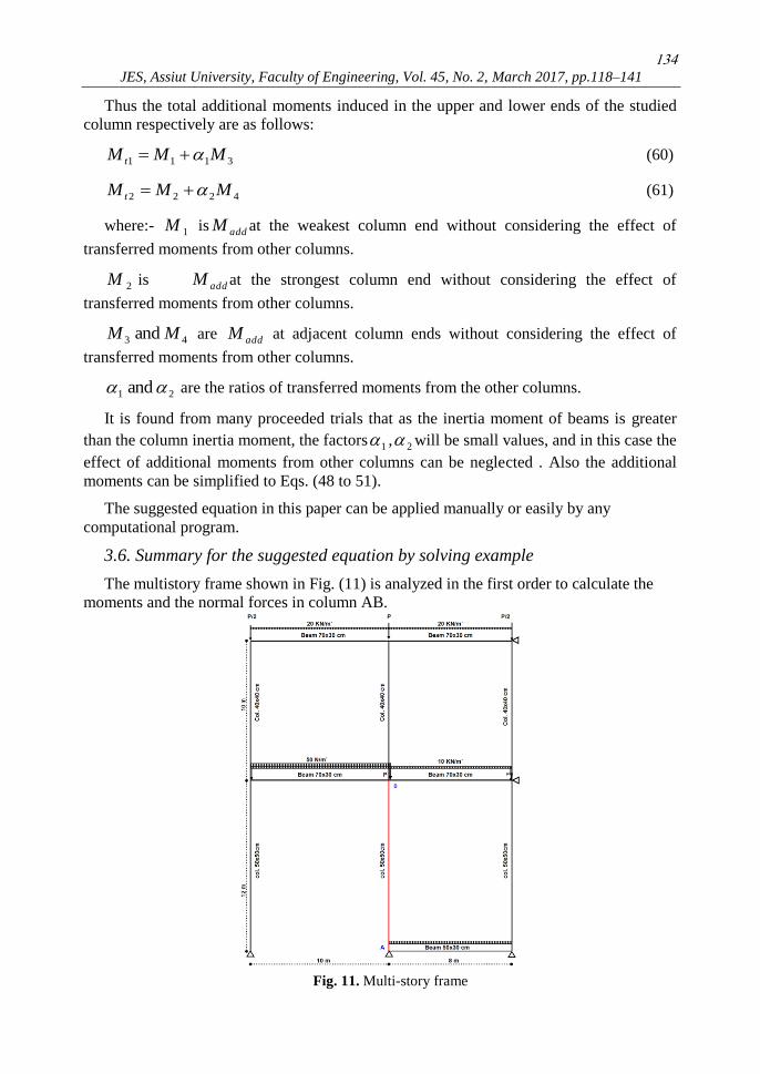
The multistory frame shown in Fig. (11) is analyzed in the first order to calculate the
moments and the normal forces in column AB.
Fig. 11. Multi-story frame
135
M. A. Farouk, second – Order analysis in braced slender columns Part 1: approximate …….
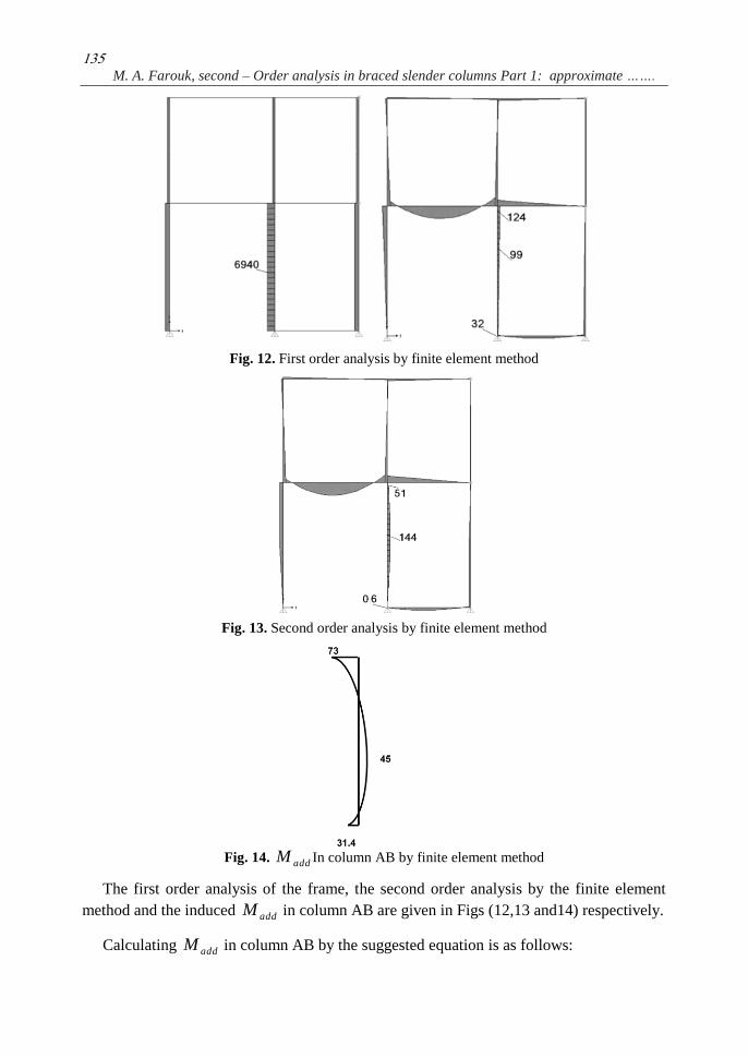
Fig. 12. First order analysis by finite element method
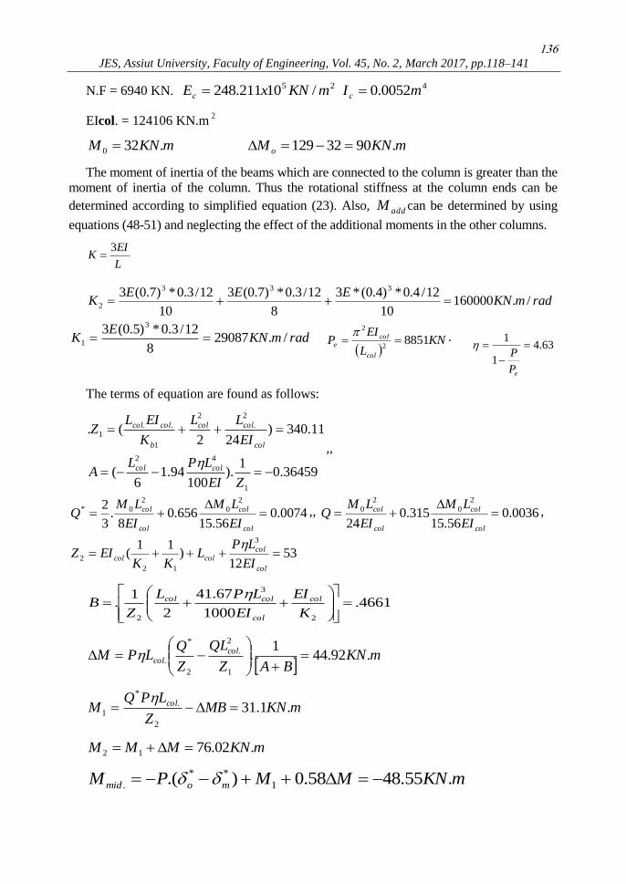
Fig. 13. Second order analysis by finite element method
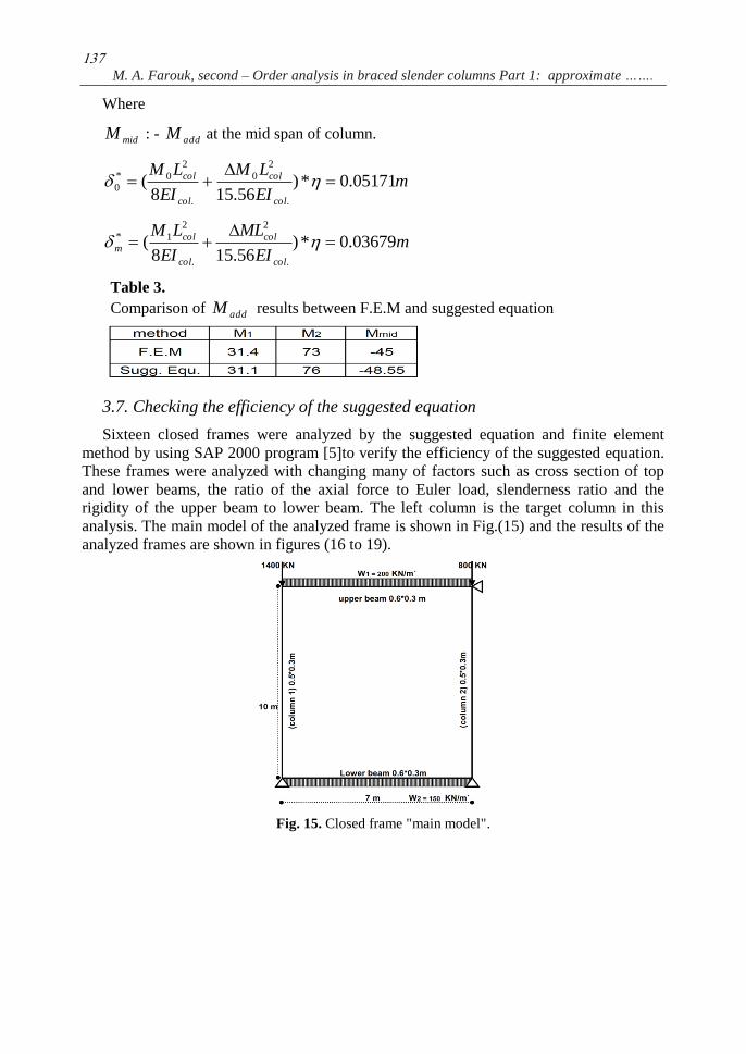
Fig. 14. addM In column AB by finite element method
The first order analysis of the frame, the second order analysis by the finite element
method and the induced addM in column AB are given in Figs (12,13 and14) respectively.
Calculating addM in column AB by the suggested equation is as follows:
136
JES, Assiut University, Faculty of Engineering, Vol. 45, No. 2, March 2017, pp.118–141
N.F = 6940 KN. 25 /10211.248 mKNxEc
40052.0 mI c
EIcol. = 124106 KN.m2
mKNM .320 mKNM o .9032129
The moment of inertia of the beams which are connected to the column is greater than the
moment of inertia of the column. Thus the rotational stiffness at the column ends can be
determined according to simplified equation (23). Also, addM can be determined by using
equations (48-51) and neglecting the effect of the additional moments in the other columns.
L
EIK
3
radmKNEEE
K /.16000010
12/4.0*)4.0(*3
8
12/3.0*)7.0(3
10
12/3.0*)7.0(3 333
2
radmKNE
K /.290878
12/3.0*)5.0(3 3
1
KNL
EIP
col
col
e 88512
2
.
63.4
1
1
eP
P
The terms of equation are found as follows:
36459.01
).100
94.16
(
11.340)242
(.
1
42
2
.
2
1
..
1
ZEI
LPLA
EI
LL
K
EILZ
colcol
col
colcol
b
colcol
,,
0074.056.15
656.08
.3
22
0
2
0*
col
col
col
col
EI
LM
EI
LMQ ,, 0036.0
56.15315.0
24
2
0
2
0
col
col
col
col
EI
LM
EI
LMQ ,
5312
)11
(3
12
2 col
col
colcolEI
LPL
KKEIZ
4661.1000
67.41
2
1.
2
3
2
K
EI
EI
LPL
ZB col
col
colcol
mKN
BAZ
QL
Z
QLPM col
col .92.441
.1
2
.
2
*
.
mKNMBZ
LPQM col .1.31
2
.
*
1
mKNMMM .02.7612
mKNMMPM momid .55.4858.0).( 1
**
.
137
M. A. Farouk, second – Order analysis in braced slender columns Part 1: approximate …….
Where
midM : - addM at the mid span of column.
mEI
LM
EI
LM
col
col
col
col 05171.0*)56.158
(.
2
0
.
2
0*
0
mEI
ML
EI
LM
col
col
col
col
m 03679.0*)56.158
(.
2
.
2
1*
Table 3.
Comparison of addM results between F.E.M and suggested equation
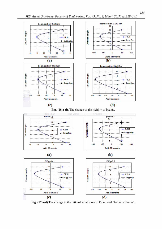
3.7. Checking the efficiency of the suggested equation
Sixteen closed frames were analyzed by the suggested equation and finite element
method by using SAP 2000 program [5[to verify the efficiency of the suggested equation.
These frames were analyzed with changing many of factors such as cross section of top
and lower beams, the ratio of the axial force to Euler load, slenderness ratio and the
rigidity of the upper beam to lower beam. The left column is the target column in this
analysis. The main model of the analyzed frame is shown in Fig.(15) and the results of the
analyzed frames are shown in figures (16 to 19).
Fig. 15. Closed frame "main model".
138
JES, Assiut University, Faculty of Engineering, Vol. 45, No. 2, March 2017, pp.118–141
Fig. (16 a-d). The change of the rigidity of beams.
Fig. (17 a-d) The change in the ratio of axial force to Euler load "for left column".
139
M. A. Farouk, second – Order analysis in braced slender columns Part 1: approximate …….
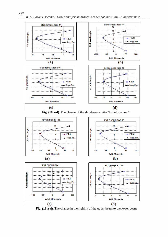
Fig. (18 a-d). The change of the slenderness ratio "for left column".
Fig. (19 a-d). The change in the rigidity of the upper beam to the lower beam
140
JES, Assiut University, Faculty of Engineering, Vol. 45, No. 2, March 2017, pp.118–141
From the results in Figs (16 to 19), it was observed that the suggested equation gives
matching results compared with that of finite element method. By the suggested equation,
we can find the additional moments at the mid length of slender columns and at the
connection between them and the connected beams. Comfortably, this equation can be
modified in future to consider stiffness reduction due to the cracks and the yielding.
4. Conclusions
The following conclusions have been drawn out of the presented study:
Approximate equation for computing the additional moments in braced slender
columns was suggested in this paper. This equation was proved in elastic
analysis and for the cases of single curvature in the slender column.
The additional moments which are induced in the slender column were
considered, not only in the mid span of the columns, but also the rigidity of the
connected beams and the induced additional moments between them and the
columns were also considered.
The suggested equation gave matching values of the induced additional moments of
the slender columns compared with the results of finite element in elastic analysis.
The suggested equation in this paper is as a prelude for the modified equation in
near future. The stiffness reduction in the column and the rotational springs due
to the cracking and yielding will be taken into account in the modified equation.
Then, the results will be compared with accredited equations in different codes.
REFERENCES
[1] ECP committee 203, (The Egyptian code for design and construction of
reinforcement concrete structures, 2007, 403P.
[2] BS8110:1997: Structural Use of Concrete Part 1: Code of Practice for Design and
Construction, 120P.
[3] Prab Bhatt, Thomas J. MacGinly and Ban Seng Choo (Reinforced Concrete,
Design Theory and Examples) Third edition, 2006,767P.
[4] Building Code Requirements for Structural Concrete (ACI 318-14),2014, 519P.
[5] SAP2000 ‘Linear and nonlinear Static and Dynamic Analysis and Design of
Three-Dimension Structures ‘ Computer and Structures, Inc. Berkeley, California,
USA Augest 2004.

141
M. A. Farouk, second – Order analysis in braced slender columns Part 1: approximate …….
إلضافية فى األعمدة النحيفة المقيدة جانبياتحليل العزوم ا
: معادلة مقترحة لحساب العزوم اإلضافية في األعمدة النحيفة األولالجزء
الملخص العربي
هذه الدراسة اختصت بتحليل العزوم اإلضافية في األعمدة النحيفة والناتجة من فعل التشكالت الحاثةكة مك
يختص بنقطتين رئيسيتين. النقطة األولي وهى إلقاء الضوء على المعاثال القوة الداخلية العموثية. هذا البحث
الموصى بها في الالوثا المختلفة والتي من ختلها يتم الحصول على العكزوم اإلضكافية المتولكدة فكي األعمكدة
لمعكاثال . ممكا النقطكة النحيفة وكيفيكة التعامكل مك هكذه المعكاثال والفكألوس واألسكب التكي بنيكت عليهكا هكذه ا
الثانية في هذا البحث هي اقتألاح معاثلة تقأليبية يتم من ختلها حسكا العكزوم اإلضكافية المتولكدة فكي األعمكدة
النحيفة. هذه المعاثلة تأخذ في االعتبار الجساءة الدورانية للالمألا بالنسبة لألعمدة والعزوم اإلضافية المتولكدة
مكألا . هكذه المعاثلكة المقتألحكة قكد تكم إةباتهكا فكي هكذا البحكث علكى مسكا التحليكل عند اتصال األعمدة بهكذه الال
المألن وفي الحاال ذا االنحنكاء األحكاثل لألعمكدة. وقكد تكم التحقكف مكن كفكاءة هكذه المعاثلكة بحكل العديكد مكن
األمثلة والحصول على نتائج متوافقة م التحليل بطأليقة العناصأل المحدوثة.