second millennium benchmark for metrohartford
TRANSCRIPT

The Second MetroHartford Regional Performance
Benchmark
By
Fred Carstensen, Director William Lott, Director of Research
Stan McMillen, Manager, Research Projects Hulya Varol, Research Assistant
Edward Zolnik, Research Assistant Na Li Dawson, Research Assistant
September 11, 2001
CONNECTICUT CENTER FOR ECONOMIC ANALYSIS
University of Connecticut 341 Mansfield Road
Unit 1063 Storrs, CT 06269-1063
Voice: 860-486-0485 Fax: 860-486-4463 http://ccea.uconn.edu

Executive Summary
The MetroHartford Growth Council has again contracted with the Connecticut Center for
Economic Analysis (CCEA) to produce a second benchmark of greater Hartford’s
regional performance. As in the first benchmark, attached as Appendix 1, we compare
MetroHartford with 55 other Metropolitan Statistical Areas that we judged to be similar
to MertroHartford.
Benchmarks have relevance to policy formation and institutional change only if they are
replicated. If the metric is meaningful, that is, it characterizes regional performance
reasonably well, then it can be used to assess the impacts of policy and other endogenous
changes, as well as exogenous shocks (national or international recessions or booms) on
the region. Untangling causes and effects of changes in benchmark results may therefore
not be easy. Our task here is simpler: replicate the first benchmark and compare results
without untangling the complicated web of causes and effects.
In the first analysis we identified 39 variables and four categories in a focus group of
economists, educators, and civic group leaders (see The First Annual MetroHartford
Benchmark, January 12, 1999 in Appendix 1). We have maintained those four categories
or concepts for grouping variables characterizing regional performance. They are:
Business Climate, Quality of Life, Human Capital, and Infrastructure. We have added
six new variables to better assess regional performance and recalculated the first
benchmark at two different dates using a different methodology. Thus we refer to the
first benchmark and two iterations of the second benchmark. The comparison below
refers to the two iterations of the second benchmark using data from different eras. The
full report compares the first and second benchmark results. The literature review
surveys recent benchmarking papers and describes the relevance of these categories as
measures of regional performance.
i

Comparing MetroHartford’s performance from the first period to the second using
current methods, we see that it slipped from 12th to 22nd in the Business Climate category,
is relatively unchanged in the Quality of Life category (19th to 23rd), and shows a
significant improvement in the Human Capital category (40th to 18th). There is some
slippage in the Infrastructure category as well (9th to 21st). The overall rank for
MetroHartford improves from 23rd to 22nd between the first and second iteration. This is
primarily attributable to the ten variables that changed from the first to the second. These
are demographic variables and are probably not good representatives for regional
performance changes per se. Moreover, MetroHartford may even have improved more
than indicated over time, but some of the 55 other MSAs improved more than
MetroHartford. For example, we know that other regions recovered sooner than
MetroHartford from the 1991/1992 recession. Connecticut has only recently recovered
the jobs it had in 1989. MetroHartford probably has not. Policies and institutional
changes effected years ago have their impacts felt only recently. That is to say that
MetroHartford has not yet felt the impact of policies such as the tax credit for brownfield
development, or the impacts of Adriaen’s Landing and other construction projects and
their resulting economic growth and fiscal enrichment. The lack of such realized changes
in MetroHartford and their evidence in other MSAs partly accounts for its relative
slippage in three out of four categories.
We focus on the seven MSAs selected for detailed policy analysis compared to
MetroHartford: Austin, TX; Harrisburg, PA; Albany, NY; Providence, RI; Des Moines,
IA; and, Raleigh-Durham, NC, and Columbus, OH (please refer to our report, ‘A Tale of
Eight Metros: Comparative Policy Analysis of MetroHartford and Similar MSAs’,
November 3, 1999). We selected these metros because they are similar in population size
and other salient characteristics to each other (state capitols, close to rivers, cultural and
educational assets).
ii

TABLE 4: Relative Ranks of Comparison Metros
BUSINESS CLIMATE QUALITY OF LIFE HUMAN CAPITAL INFRASTRUCTURE OVERALL
1994 1996 1994 1996 1994 1996 1994 1996 1994 1996
Raleigh-
Durham(1)
Austin(1) Austin(4) Des Moines
(1)
Austin(1) Raleigh-
Durham(1)
Raleigh-
Durham(2)
Raleigh-
Durham(5)
Raleigh-
Durham(1)
Raleigh-
Durham(1)
Des
Moines(4)
Raleigh-
Durham(2)
Des
Moines(5)
Austin (2) Raleigh-
Durham(2)
Austin(2) Hartford
(9)
Columbus
(15)
Austin(2)
Austin(2)
Hartford
(12)
Des
Moines(10)
Harrisburg
(9)
Harrisburg(9) Des
Moines(3)
Columbus
(3)
Albany(19) Hartford(21) Des
Moines(3)
Des Moines(6)
Providence
(18)
Hartford (22) Hartford
(19)
Raleigh-
Durham(11)
Columbus
(4)
Des Moines
(4)
Des
Moines(27)
Albany(26) Columbus
(10)
Columbus(10)
Austin(21) Providence(24) Raleigh-
Durham(20)
Albany(16) Harrisburg Hartford(18)
(17)
Harrisburg
(30)
Austin(30) Harrisburg
(14)
Hartford(22)
Harrisburg
(23)
Columbus (26) Columbus
(23)
Columbus(21) Albany
(18)
Albany(21) Columbus
(32)
Providence
(38)
Hartford
(23)
Harrisburg(27)
Columbus
(25)
Harrisburg(30) Albany(27) Hartford(23) Hartford
(40)
Harrisburg
(27)
Providence
(34)
Harrisburg
(41)
Albany
(27)
Albany(31)
Albany
(50)
Albany (48) Providence
(30)
Providence(28) Providence
(41)
Providence
(41)
Austin(37) Des
Moines(45)
Providence
(36)
Providence(37)
iii
Table 4 above shows the relative ranks of the eight metros in both benchmark studies.
The ranks arise from a composite rank for each category and overall ranks based on
average scores (see Tables 5 and 6 below). The important observation from this portrayal
is that Austin, Raleigh-Durham and Des Moines rank consistently higher than Hartford,
Albany and Providence. Albany and Providence appear lower ranked than Hartford in
several categories across both benchmarks. The detailed comparison of these metros
suggests the many development, structural, political and jurisdictional differences among
them that account in part for their relative ranking.
MetroHartford has apparently fallen behind some of its competitors over the last few
years according to the metric established to assess its performance. This is accountable
by its later recovery from the early 1990s recession, its paucity of development projects
relative to other areas (see the comparative cities report cited below) in the middle 1990s,
and, the lag of the effects of (local) policy and institutional changes. It is essential that
local changes be recorded and described such that their effects can be tracked via the
benchmark process. There are lags as well in the effects of economic development,
policy and institutional changes as they manifest in the benchmark variables we assemble
(some variables are annual, others biannual, quadrennial, and some, decennial).
Future work will employ more sophisticated time series analysis (dynamic factor
analysis) to create more objective variable weights and have greater temporal stability.
iv

Literature Review I. Introduction Measuring the performance of metropolitan areas in the U.S. has been an important topic
for state and local governments, policy makers, business firms, and individuals in recent
years. One of the major goals of state and local governments is to develop their cities and
towns in a way that makes them attractive not only to individuals but also to business
firms. Few cities or towns can thrive without business activity to increase employment,
income tax revenues, and the overall welfare of its residents. Because business firms are
central players in the development of a city or town, policy makers can design policies
that attract business firms to locate in the area by enhancing factors such as business
climate, quality of life, infrastructure, and the availability and quality of human capital.
Most often, the decision of individuals and firms to locate in a particular area may largely
depend upon existing information regarding that particular region or location. There are
several sources by which individuals and business firms can access relevant information
about a town or city. Some of the popular sources of information are rankings of towns,
cities and Metropolitan Statistical Areas (MSAs) in the U.S. published by business
institutions and popular media. These comparisons rank towns and cities in the U.S.
annually on the basis of some key socio-economic factors such as crime, housing,
education, employment, air quality, economy, leisure activities and the arts. This type of
ranking of town and cities, however, may not accurately reflect the true business and
living climates of the towns and cities under consideration. The reason is that when
ranking towns and cities these studies construct an overall index created by assigning
different weights to different factors depending upon the perceived significance of each
factor to the investigator. There is no general consensus or set of rules that precisely
postulates what factors should be taken into account and how much weight should be
given to each factor. As a result, the conclusions of these studies are often different, even
contradictory. For example, the results from a study of a town or city focusing on
individual preferences may be completely different from a similar study focusing on the
preferences of business firms. For the former, pleasant weather, excellent schools and
colleges, proficient hospital care and low living costs are some of the most important
1

factors; for the latter, low corporate taxes, highly developed and well-maintained
infrastructure, high quality human capital, and sophisticated communication networks are
crucial.
Another drawback of these studies is that some of the factors included in the studies are
static and thus can not explain trends and potential changes in the factors. For example,
policy variables such as sales tax, property tax, public spending on education and
infrastructure are endogenous factors that state and local governments control. These
kinds of policy variables can easily change over time and are likely to affect other factors
as well. A state or local government with a positive attitude toward business could imply
liberal sales and property tax policy in the future. This may in turn lead to a more
favorable business climate for firms and a higher quality of life for residents. As a result,
given the potential changes in state and local government policies, today’s lowest rated
town may not necessarily remain so in a few years and vice versa. This means that
ranking MSAs based solely on static quantities fails to predict meaningfully how changes
in the policies of a state or local government might significantly affect the existing
business climate, quality of life and other factors in a particular MSA over a period of
time. In such circumstances, it is critical for business firms to exercise good judgment
about the potential changes in the business environment due to changes in the policies of
state and local governments before they make a final decision on where to invest.
Similarly, the role of state and local governments becomes equally important in attracting
more business firms by reevaluating existing policies and designing more favorable ones.
Few studies have attempted to focus specifically on examining the performance of cities
or MSAs over a period of time. A study measuring relative performance of MSAs over a
period of time using appropriate statistical tools may therefore provide more reliable and
accurate information for business firms and individuals. In addition, understanding the
changes in economic performance of an MSA over time can help policy makers shape
future infrastructure investment and social and economic development policy. This
literature review investigates earlier studies evaluating and measuring the performance of
MSAs in the U.S. during the past few years in an attempt to provide a background for
2

consistently and accurately evaluating MSAs relative to one another and themselves over
time.
II. Literature Review Discussion about which cities in the U.S. have performed relatively well and whether city
residents have benefited is limited. In addition, each study uses different data and criteria
to analyze cities and so there are as many different results as there are studies. In general,
however, one can view the performance of a city in terms of improvement in a variety of
economic, social and physical conditions such as increased business investment, physical
redevelopment, reduction in crime and infant mortality rates, and increases in educational
achievement and human capital.
It is important for policy makers to examine which MSAs are growing fastest and which
are experiencing slower growth and investigate the reasons for differing growth rates
among them. An index of economic performance can be a useful tool to measure the
relative performance of cities. Coomes and Olson (1990) attempt to develop a
methodology to measure the economic performance of metropolitan areas in the United
States. Their motivation for constructing an economic performance index is to measure
economic performance in a timely basis and examine the value of jobs lost or created in
the MSA during a specific time period. A good proxy for the economic performance of
cities is the personal income data produced by the Bureau of Economic Analysis (BEA).
However, this data is only available with a two-year lag. To overcome this and be able to
measure the recent economic performance of cities the authors construct an economic
performance index that combines the timeliness of the job data with the completeness of
wage and income data to provide a measure of recent economic growth in urban areas.
The earnings data mainly consists of wages and salaries, while income data consists of
income other than wages and salaries, e.g., rent and profit. The index is then constructed
by weighting total jobs in each industry in a city using monthly Bureau of Labor
Statistics (BLS) data of the latest available estimates of average annual earnings for that
industry in that city (using historical BEA data). In other words, the earnings-weighted
job data construct an economic performance index to compare economic growth among
3

metropolitan areas. Coomes and Olson use 1990 as a base year, rather than current
earnings weights, to construct their economic performance index, which reflects real
earnings growth. The methodology to construct the economic price index is similar to
that used to construct the U.S. Consumer Price Index, or CPI. The index constructed for
metropolitan area j in time period t is:
EPIjt = 100*
1.
1.
∑
∑
=
=n
iiBiB
n
iitiB
JE
JE,
where Jit and JiB are the number of jobs in industry i in the period t and base period B
respectively. Similarly, EiB represents the average earnings or wages in metropolitan area
industry i (i =1,2,...n) in the base period. To lessen the impact of seasonality and
problems arising from occasional outliers, the authors chose to use average metropolitan
area earnings by industry over the most recent three years as the weights, EiB (Coomes
and Olson 1990).
Coomes and Olson (1990) then compare the economic performance index with other
measures of economic growth. They find that the ranking of cities based on an economic
performance index (earning income growth) and personal income growth are quite
different in high cost of living areas. For example, Boston ranked 7th in terms of
personal income growth and 60th in terms of earnings growth. Similarly, Hartford
ranked 17th in terms of personal income growth and 65th in terms of earnings growth.
The authors also point out the geographic incompatibility between the BLS and BEA data
set in the six New England states in which MSAs are not limited to one state. For
example, the Boston CMSA (Consolidated Metropolitan Statistical Area) is composed of
six PMSAs (Primary Metropolitan Statistical Area), of which the Nashua PMSA belongs
to New Hampshire. PMSAs consist of a large urbanized county or cluster of counties
that demonstrate strong internal economic and social links in addition to close ties to
other portions of the larger area. The CMSA is as a larger area that consists of several
PMSAs. Monthly BLS job data for the PMSAs aggregates to arrive at Boston CMSA
totals. However, the BEA annual earnings data for the Boston NECMA (New England
4
Consolidated Metropolitan Area) refer to the sum over five Massachusetts counties. To
solve this problem, the authors drop the Nashua PMSA job data from the calculation of
job growth in the NECMA.
In another study, Duncomber and Wong (1997) attempt to measure the trend of economic
performance of Onondaga County, New York, and compare the county’s performance to
other metropolitan areas and regions in New York State and several fast growing MSAs
in the South. They do not construct any kind of measurement index; rather, they simply
look at the trend in some key economic indicators of Onondaga County and compare
these indicators to other regions in New York. The key economic indicators used in their
study include income, employment, earnings and wages. More specifically, they look at
the source of income growth, the composition of employment growth, changes in
employment structure and structural changes in earnings. They also measure the
competitiveness of local industries by using a location quotient that compares the relative
size of an industry in a local area to that industry’s share of national employment. This is
a measure of industry mix and captures an element of regional economic stability.
Other studies attempt to test the outcomes of earlier studies that measured the
performance of MSAs. Wolman, Ford, and Hill (1994) evaluate some earlier studies
regarding the performance of MSAs between 1980 and 1990 and question the story of so-
called “successful cities” in the U.S. They focus on the economic wellbeing of some
cities that have undergone urban revitalization. By developing their own urban distress
index using the unemployment rate, poverty rate, median household income, percentage
change in per capita income and percentage change in population, they compare the
economic wellbeing of the residents of the target cities. They make comparisons between
twelve ‘successfully revitalized cities’ and the 38 other ‘unsuccessful cities’. They find
the ‘unsuccessful’ cities on some of the indicators actually outperformed ‘successfully’
revitalized cities. The ‘unsuccessful’ cities did better in terms of the unemployment rate
and greater improvement in median income than the ‘successful’ cities.
5
Wolman, Ford and Hill (1994) also construct an overall index of economic well being as
a summary measure of the change in resident economic wellbeing from 1980 to 1990.
The index is constructed by summing the standard scores of the five indicators
(percentage change in each of the following: unemployment rate, labor force participation
rate, poverty rate, median household income and per capita income). They also find that
the ‘unsuccessful’ cities outperformed the ‘most successfully revitalized’ cities on all of
the five indicators of resident wellbeing.
They also suggest possible future research by examining the factors that account for the
performance of those distressed cities that actually improved the economic wellbeing of
their residents. Two important questions that arise in their study are what factors
accounted for superior city performance and to what extent can that performance be
attributed to policy choices made by these cities, rather than to regional and national
economic factors. They also suggest that by using the same data set, it is possible to
examine the relative performance of central cities and their metropolitan areas.
There are a few other studies that attempt to identify the specific factors that largely
determine the growth and performance of MSAs. One study by Gittell (1992) examines
the effect of public, private, and community based local economic development
initiatives on the local economic performance of four medium sized, declining cities in
the northeast United States: Lowell and New Bedford, MA, Jamestown, NY, and
McKeesport, PA. Using shift-share analysis, which distinguishes between national and
regional effects on local growth, this study measures the difference in local economic
performance as measured by employment change, and also compares the city’s
performance relative to the state’s. The study finds that Lowell, compared to New
Bedford, achieved significant employment growth in the late 1970s and early 1980s even
after considering industry mix, production costs, and other factors. Similarly,
Jamestown, compared to McKeesport, experienced significant economic vitality in the
1970s that can not be fully explained by regional economic change, industry mix and
factor costs. These findings suggest that the late 1970s and early 1980s in Lowell and
New Bedford and the 1970s in Jamestown and McKeesport might be particularly useful
6

time periods to look beyond shift-share and other traditional regional development
factors, and to focus instead on the potential role of local development initiatives in these
cities.
A study by Cadwallader (1991) analyzes the factors determining metropolitan growth and
decline in the U.S. He attempts to explain the variation in growth rates among cities by
focusing on the role of migration. He uses discriminant analysis, which identifies the
major variables that differentiate between growing and declining urban areas. Similarly,
by using a simultaneous equation model, he examines the interrelationships between
migration rates for cities and other variables such as income, unemployment, taxes,
public spending, housing costs, crime rate and climatic attractiveness, which are all
proxies for quality of life. He finds a substantial difference between growing and
declining cities in manufacturing employment, with declining cities being more heavily
oriented towards manufacturing activity. His study finds that housing costs and various
kinds of local taxes are uniformly higher for the declining cities. In contrast, he finds
similarities in the two groups of cities in terms of local government expenditures, with
growing cities having slightly higher rates for the first period, but slightly lower rates for
the second period. Cadwallader argues that manufacturing activity and taxes contribute
most to the discriminating function, while spending on education makes a somewhat less
important contribution to the discriminating process. Similarly, using simultaneous
equation models, he finds a negative relation between property taxes and net migration,
but a positive relation between educational spending and housing values.
The evaluation of particular MSAs by incorporating both economic and non-economic
factors is likely to draw an overall picture of the MSA. However, it is hard to make any
kind of judgment on a location decision for business firms or individuals without
specifically looking into the most critical factors that describe their preferences. From
the point of view of a business firm, business climate, infrastructure and human capital
are the major factors that influence its location decision, while from an individual point
of view, quality of life is the most important factor. A focus group of economists arrived
at the conclusion that these four major categories, (business climate, human capital,
7

quality of life and infrastructure) taken together, can be considered to encompass the
main factors that largely influence the location decisions of both enterprises and
individuals. There are some studies that attempt to evaluate MSAs on the basis of each
of these factors separately. The following section will briefly review these factors and
explore the earlier studies that mainly focus upon these factors.
Business Climate Business climate is one of the most important factors that determine the location of
business enterprises. What constitutes a favorable business climate is not entirely clear,
but it is usually associated with suitability of investment, low state and local taxes,
amenable right to work laws, little union activity and a cooperative governmental
structure (Plaut and Pluta, 1983). Because the objective of firms is to maximize profit
with minimum risk, selection of a location with a favorable business climate is of central
importance.
Business climate can be best reflected by factors such as cost of doing business, access to
markets, and corporate and property tax rates. Other factors listed by some business
magazines that may also represent business climate include government attitude toward
business, business performance, (as measured by company failure rates and payment
delinquencies), economic growth (employment growth and growth in the average wage
per job), risk (the chances of business failure over the next 18 months, the amount of time
in business, history of principals, and record of paying suppliers) and affordability
(increases in the cost of living index, as well as growth in wages).
On the basis of some key factors that represent business climate, some business
magazines (e.g., Financial World, Fortune, Site Selection, and Entrepreneur) produce
rankings of metropolitan areas in the U.S. The rankings in Financial World are based on
four common yardsticks: major services, financial strength, tax status and operating tools.
The Fortune magazine rankings have been the most popular among business firms and
are widely used. They are based on a survey of more than 1000 U.S. business executives
8

on business costs, availability and skills of workers, cost of workers, social conflicts,
transportation and other factors in different metropolitan areas of the U.S.
Because most of these studies have their own methodology and criteria to produce
rankings, they are not directly comparable to each other. Some studies are based only on
hard statistics, while others are based on subjective input such as survey responses. Some
studies use a combination of both. Furthermore, these studies differ significantly from
each other in terms of the economic and social factors being measured. As a result, it is
not an easy task to judge which of these studies is the most reliable or suitable to a
location decision.
Among other studies, Grant Thornton (1986) produces rankings of manufacturing
climates of the forty-eight contiguous states in the U.S. Grant Thornton’s ranking system
is somewhat different from the other ranking systems. In his study, a state is considered
to be “manufacturing intensive” if it has contributed an average of more than 2 percent of
the value of manufacturing shipments in the country over the last four years or has had an
average of 16.5% or more of its work force engaged in manufacturing over the last four
years (this percentage is the four-year national average, according to Bureau of Labor
Statistics data). However, some researchers on a number of grounds have criticized the
Grant Thronton rankings.
Lane, Glennon, and McCabe (1989) analyze the volatility of the Grant Thornton rankings
and the relationship between states’ rankings and gross state product. They use cluster
analysis to determine the underlying similarity of states and to determine whether the
factors used by Grant Thornton provide insight into the best and worst performing states.
By sucessively regressing percentage change in output of manufacturing industries,
percentage change in GSP, and GSP level on a ranking of states by business climate
produced by Grant Thornton, they find virtually no relationship between ranking of states
by business climate and actual health of the manufacturing sector measured by output
data available from BEA. They suggest that the actual growth rates of states as a
measure of business climate makes more sense than some artificial construction.
9

Other than ranking MSAs or states by business climate, there are some studies that
attempt to link the business climate with state industrial growth in the U.S. as well. A
study by Plaut and Pluta (1983) tests the relationship between a wide range of both non-
economic and economic factors including business climate and multiple measures of
industrial growth. Using principal components analysis and a multiple regression model
on pooled data for forty-eight contiguous states, they test the effects of four groups of
variables (accessibility to markets, cost and availability of factors of production, climate
and environment, and business climate and state and local taxes and expenditures) on
three separate measures of industrial growth. Among other findings, their study shows
that business climate, tax, and expenditure variables, as a group, were significantly
related to state employment and capital stock growth. Similarly, poor business climate
and high tax rates both appear to have a negative effect on employment growth.
Quality of Life Quality of life is one of the most critical, and also one of the most nebulous, factors in the
location decision for individuals. For business firms this factor is equally significant if
not dominant when making location decisions. While the quality of life can be defined in
several ways, it mainly implies the wellbeing of people as determined by health, welfare,
freedom of choice, availability of food, clothing and shelter, educational facilities,
security and income.
The issue of quality of life has been adequately analyzed in the literature. Developing a
methodology to measure quality of life, however, has not been easy. The major problem
for researchers in constructing a quality of life index has been developing a method for
weighting different amenities. Some researchers produce quality of life indexes by
weighting amenities in an atheoretic manner (Liu, 1976), and some develop a bundle of
wages, rents, and amenities (Rosen, 1979).
10

Blomquist, Berger, and Hoehn (1988) construct a quality of life index by incorporating
wages and rent effects. They allow for amenity variation both within and across urban
areas. They argue that agglomeration effects due to productivity effects of city size
provide a key linkage between firms of given urban areas. They estimate hedonic rent
and wage equations using 1980 U.S. Bureau of Census data matched with amenity data
on climatic, environmental, and urban conditions. Using a hedonic model, they estimate
implicit amenity prices and weigh them in a quality of life index that is computed for 253
urban counties within 185 MSAs in the U.S. The hedonic model disaggregates the prices
of the goods into more basic units (the characteristics) and provides estimates of prices
for the characteristics.
A study by Kahn (1995) develops a new method for ranking city by quality of life. Using
a revealed preference approach, he finds that Los Angeles and San Francisco had higher
quality of life than Chicago and Houston in both 1980 and 1990 and that the quality of
life in New York City fell during the 1980s.
Human Capital While business climate and quality of life remain important factors that affect both
business firm’s and individual’s choice of location, availability of human capital in a
particular location is another factor that significantly affects the location decisions of
business firms. Without skilled human capital, other physical and financial capital
becomes less productive. In recognition of the fact that the availability of human capital
can therefore be considered an important aspect of business climate, there are several
studies that primarily focus on human capital and its impact on the growth and
performance of MSAs in the U.S.
In a 1988 paper, Lucas rightly argues that economic growth depends crucially on the
ability to absorb existing knowledge and create new knowledge, both of which are
directly related to the existing stock of human capital and both of which may be more
costly the more geographically distant the source of human capital. Cities in which firms
can communicate more cheaply with people whose job it is to absorb, create, transmit,
11

and implement knowledge - that is, cities with greater concentrations of highly educated
individuals - should become relatively more productive and, hence, attract population at a
faster rate. Access to educated individuals is particularly important in a world of
technical change, much of which has been biased in favor of individuals with higher
levels of skill. In addition, cities with higher concentrations of educated individuals
should also generate more localized spillovers.
In various studies, human capital is usually measured in terms of some measure of
educational level. For example, the percentage of the population who have graduated
from high school, the percentage of the population who have graduated from college, the
mean or median years of total education, or a combination of these are generally used as
a measure of human capital. As noted by Simon (1998), however, no studies dealing
with human capital and the economic performance of MSAs have attempted to adjust
these scales for the quality of education received. This may be an important factor in
accurately measuring human capital in an area.
Most of the studies done related to human capital primarily focus on the impact of human
capital on the growth and development of MSAs. However, almost no study has
attempted to measure or rank the performance of MSAs solely on the basis of human
capital.
In a recent study, Simon (1998) attempts to test empirically the relationship between
human capital and metropolitan employment growth in MSAs in the U.S. Using data on
all U.S. MSAs for the period of 1940-86, he finds a robust positive relationship between
average level of human capital and employment growth. In the same paper, Simon also
examines the spillover effects of human capital between cities within MSAs. He finds
that there exists a definite positive relationship between human capital elsewhere in an
MSA and employment growth within a city of an MSA. However, he also finds that the
relationship is limited – human capital existing within the city causes higher economic
growth in the city than human capital from other areas within the MSA. Hence, the
spillover effects exist, but the benefits tend to be spatially specific.
12

Infrastructure The last important category in measuring the status and relative performance of MSAs in
the U.S. over the past few years is infrastructure. Sufficient investment in infrastructure
is widely recognized as necessary to economic development and an important indicator of
economic growth. In recognition of this, many studies have examined the link between
investment in infrastructure and economic performance. No studies have attempted to
rank MSAs based on infrastructure alone, however. The literature examining the various
components of infrastructure and the effects of infrastructure investment on economic
performance provides some useful information and conclusions nevertheless. As
expected, the conclusions vary because the exact components of infrastructure studied
and the relative importance assigned to them varies from study to study.
The term infrastructure generally refers to the underlying network supporting the
activities of the city or MSA being studied. As noted by Cain (1997), older studies of
infrastructure focused mainly on transportation (railroads, roads, canals and highways)
and sanitation (both water supply and sewage removal) in measuring infrastructure.
More recently, however, non-transportation or sanitation factors such as the availability
of education, health facilities, energy, and communications systems have been added into
the infrastructure equation. All of these factors are considered to have both direct and
indirect effects on economic performance. Infrastructure can affect production as well as
the productivity of labor and private capital directly, or can have an indirect effect by
attracting labor and private capital from other areas (Bell et al, 1997).
Although the literature examining infrastructure varies with respect to its focus and the
data and approach used, most studies of infrastructure and its effects on economic
progress show a positive relationship between the two. A study by Aschauer (1989)
examines the individual effects of investing in infrastructure, labor, and private capital on
economic performance. Using an aggregate production function and time series data for
the U.S. from 1949-85, he concludes that investment in infrastructure has not only a
positive effect on economic performance, but a greater effect than that of investing in
13
either labor or private capital. In the same paper, Aschauer also looks into the relative
effects of the various components of infrastructure. In this area he concludes that
investment into ‘core’ infrastructure such as transportation, energy, water and sewage
systems has a greater positive effect on economic performance than investment into other
components of infrastructure such as hospitals and buildings.
Numerous other studies find relationships between specific individual components of
infrastructure and the relative ‘attractiveness’ of areas in terms of location decisions,
though none specifically rank cities or MSAs according to these components. For
example, in a state-level study Fox and Murray (1990) conclude that the availability of
interstate highways is a major factor in determining where firms locate, while Fox,
Herzog and Schlottman (1989) find that the quality of infrastructure services positively
affects residential migration to an area.
III. Conclusion
Measuring the performance of metropolitan areas in the U.S. has been and continues to
be an important issue for state and local governments, policymakers, firms and
individuals alike. Several studies have attempted to rank MSAs relative to one another
on the basis of one to many different factors. However, the factors considered to be
important vary from one study to the next and as a result no consistent set of criteria to be
considered has emerged. In addition, few studies have attempted to measure the relative
performance of MSAs over time. The presence of these limitations in the current
research provides a promising direction for further research. This literature review has
attempted to provide a background useful for designing a methodology to measure the
status and relative performance of MSAs in the U.S. over time by focusing on four major
categories that affect regional economic performance and hence influence firm and
individual decisions to locate in an area. These categories are business climate, quality of
life, human capital and infrastructure. Each one is an important part of a consistent,
comprehensive system for analyzing MSAs relative to one another and to themselves
14

over time. By carefully considering the important components and relative importance of
each of these factors, a consistent and successful measure of MSAs relative to one
another and to themselves over time may emerge. This review has attempted to provide
the background necessary for such an endeavor.
15

References
Aschauer, D. (1989) “Is Public Expenditure Productive,” Journal of Monetary
Economics, Vol. 23, pp 177-200.
Bell, M., McGuire, T. et al (1997) “Macroeconomic Analysis of the Linkages Between
Transportation Investments and Economic Performance”, National Cooperative
Highway Research Program Report No. 389.
Blomquist, G., Berger, M., Hoehn, J. (1988) “New Estimates of Quality of Life in Urban
Areas”, The American Economic Review, Vol.78, No. 1, pp 89-107.
Cadwallader, M. (1991) “Metropolitan Growth and Decline in the United States: an
Empirical Analysis”, Growth and Change, Summer, pp. 1-16.
Cain, L. (1997) “Historical Perspective on Infrastructure and US Economic
Development”, Regional Science and Urban Economics, 27, pp. 117-138
Coomes, P. and Olson, D. (1990) “Using BEA and BLS Data to Monitor Metropolitan
Area Economic Performance” Journal of Economic and Social Measurement, 16,
pp. 167-183.
Crihfield, J. and McGuire, T. (1997) “Infrastructure, Economic Development, and Public
Policy”, Regional Science and Urban Economics, 27, pp. 113-116.
Duncomber, W. and Wong, W. (1997) “Onondaga County’s Economic Performance
Since 1980 and Prospects for the Next Decade,” Metropolitan Studies Program
Series Occasional Paper No. 183.
Fox, W., Herzog, H. and Schlottman, A. (1989) “Metropolitan Fiscal Structure and
Migration”, Journal of Regional Science, Vol. 29, pp. 523-536.
Fox, W. and Murray, M. (1990) “Local Public Policies and Interregional Business
Development”, Southern Economic Journal, Vol. 57.
Gittell, R. (1992) “Renewing Cities”, Princeton University Press, Princeton, New Jersey.
Grant Thornton (1986) “General Manufacturing Climates of the Forty-Eight Contiguous
States of America”, Chicago, June.
Kahn, M. (1995) “A Revealed Preference Approach to Ranking City Quality of Life”,
Journal of Urban Economics, 38, pp. 221- 235.
16

Lane, J., Glennon, D., and McCabe, J., (1989) “Measures of Local Business Climate:
Alternative Approaches”, Regional Science Perspective, Vol. 19(1), pp. 89-106.
Lucas, R.E. Jr., (1988) “On the Mechanics of Economic Development”, Journal of
Monetary Economics, 22, pp. 3-42
Liu, B.C., (1976) “Quality of Life Indicators in U.S. Metropolitan Areas,” New York:
Praeger Publishers.
Plaut, T. and Pluta, J., (1983) “Business Climate, Taxes and Expenditures, and State
Industrial Growth in the United States,” Southern Economic Journal, July, pp. 99-
119.
Rosen, S., (1979) “Wage-Based Indexes of Urban Quality of Life” in Peter Mieszkowski
and Mahlon Straszheim, eds., Current Issues in Urban Economics, Baltimore: Johns
Hopkins University Press.
Simon, C., (1998) “Human Capital and Metropolitan Employment Growth”, Journal of
Urban Economics, 43, pp. 223-243
Wolman, H., Ford, C. and Hill, E., (1994), “Evaluating the Success of Urban Success
Stories”, Urban Studies, 31, June, pp. 835-850
17

Second Millennium Benchmark for MetroHartford Introduction
The MetroHartford Growth Council has contracted with the Connecticut Center for
Economic Analysis (CCEA) to produce a second benchmark of greater Hartford’s
regional performance. Our geography of interest is the Hartford Metropolitan Statistical
Area and our timeframe is 1999 or the most recently available data. As in the first
benchmark, attached as Appendix 1, we compare MetroHartford with 55 other MSAs that
we judged to be similar to MertroHartford on a population basis (500,000 to 1,500,000
people), and in spatial and economic structure.
Benchmarks have relevance to policy formation only if they are replicated. If the metric
is meaningful, that is, it characterizes regional performance reasonably well, then it can
be used to assess the impacts of policy and other endogenous changes, as well as
exogenous shocks (national or international recessions or booms) on the region.
Untangling causes and effects of changes in benchmark results may therefore not be easy.
Our task is simpler: replicate the first benchmark and compare results without untangling
the complicated web of causes and effects.
In doing so, we noticed that slight changes in a few variables altered the (static factor
analysis) results of the first benchmark significantly. Comparability across time therefore
becomes untenable with the first approach. We needed a different approach that would
ensure comparability across time to have a useful metric. A traditional approach is to use
linear combinations of variables that characterize regional performance. These
combinations may have equally weighted variables or subjectively weighted variables.
The advantage of this approach is stability (comparability) across time. The disadvantage
is that a weighting scheme introduces bias, ostensibly absent in the statistical factor
(latent variable) analysis used in the first benchmark. Given these tradeoffs and the
simplicity of linear combinations (latent variables always introduce interpretational
problems), we chose linear combinations as our primary methodology. We therefore had
18

to redo the first benchmark using linear combinations. Given this opportunity, we added
six new variables to the mix (see Methodology below) to enhance our characterization of
regional performance. The difference between the two benchmarks is the dates of the
variables.
Methodology
As mentioned, our methodology in the first benchmark was factor analysis, a statistical
technique that uncovers latent variables around which several observed variables cluster
in relation to their statistical correlation. The latent variables or factors can be interpreted
as concepts or characteristics of an abstract phenomenon such as regional performance or
manufacturing competitiveness. In the first analysis we identified 39 variables and four
categories in a focus group of economists, educators, and civic group leaders (see The
First Annual MetroHartford Benchmark, January 12, 1999 in Appendix 1). We have
maintained those four categories or concepts for grouping variables characterizing
regional performance. They are: Business Climate, Quality of Life, Human Capital, and
Infrastructure. Business Climate includes such variables as per capita housing starts; real
income growth per capita; government, manufacturing and white collar shares of
employment; corporate tax burden; output per capita; employment growth in
manufacturing, construction and white collar sectors; and, the bankruptcy rate. Human
Capital includes such variables as total population; its growth rate; the dependent
population ratio (under 12 and over 65); labor force participation rate; unemployment
rate; percent foreign born; percent with high school diploma or GED; and, percent with
college degree. Quality of Life includes such variables as percent population in poverty;
percent female-headed households; air quality index; death rate; birth rate; heating and
cooling degree days; housing affordability index; violent and property crime rates; and,
the single family home price growth rate. Infrastructure includes such variables as FAA
airport classification; hospital beds per capita; land areas; number of interstate highways;
physicians per capita; population density; and, patents per capita. Appendix 2 contains a
complete list of the 45 current variables in each category. The earlier factor analysis
produced three meaningful factors or categories we called: Economic Vitality, Quality of
19

Life, and Socio-Economic Productivity. We felt comfortable with these as reasonable
approximations to our original group of four categories until we replicated the benchmark
using later data. Only a few variables changed and these only slightly, but the impact on
the factor analysis was significant. These perturbations elicited different factors and
correlations (weights) than in the first analysis and rendered comparability impossible.
We decided therefore to use linear combinations of variables artificially grouped into our
four original categories. We would use equal weights, subjective weights and weights
suggested by the factor analysis (discretion was used in assigning these) to generate
rankings by category and overall for the earlier dated variables and for the most recently
available (1999) data set [not all variables are available at the same date].
As the term implies, equal weighting applies a weight of 1/n (n=number of variables)
applied to each variable in calculating their scores. The process works as follows: in each
category, each variable for the 56 MSAs is assumed to come from a normal distribution
for which we calculate the sample mean and variance; and, the cumulative probability
(score) for each variable for each MSA in each category is calculated. We average (or
total) the scores for the variables in each category and their score in each category ranks
each MSA. We sum category scores and produce overall ranks. For the weighted cases,
we apply the weights to the total scores (cumulative probabilities) of the variables and the
weighted average scores rank the MSAs.
For the subjective weights, we calculated the agreement of the ten respondents to the
weighting exercise (the survey form is in Appendix 2). Using Kendall’s measure of
concordance (with no ties), the test statistic is 3.52 (P<0.0002). Therefore, we reject the
null hypothesis of no agreement among the respondents. We looked at measures of
agreement among the three ranking schemes. According to Table 1, there is substantial
pairwise agreement between the methods and overall for both data sets (Phase 1 is the
earlier data set).
20
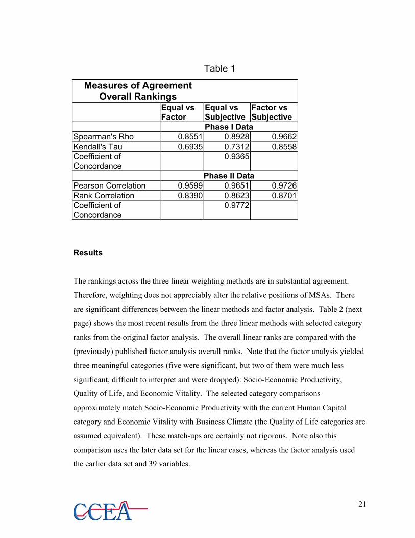
Table 1
Measures of Agreement Overall Rankings
Equal vs Factor
Equal vs Subjective
Factor vs Subjective
Phase I Data Spearman's Rho 0.8551 0.8928 0.9662 Kendall's Tau 0.6935 0.7312 0.8558 Coefficient of Concordance
0.9365
Phase II Data Pearson Correlation 0.9599 0.9651 0.9726 Rank Correlation 0.8390 0.8623 0.8701 Coefficient of Concordance
0.9772
Results
The rankings across the three linear weighting methods are in substantial agreement.
Therefore, weighting does not appreciably alter the relative positions of MSAs. There
are significant differences between the linear methods and factor analysis. Table 2 (next
page) shows the most recent results from the three linear methods with selected category
ranks from the original factor analysis. The overall linear ranks are compared with the
(previously) published factor analysis overall ranks. Note that the factor analysis yielded
three meaningful categories (five were significant, but two of them were much less
significant, difficult to interpret and were dropped): Socio-Economic Productivity,
Quality of Life, and Economic Vitality. The selected category comparisons
approximately match Socio-Economic Productivity with the current Human Capital
category and Economic Vitality with Business Climate (the Quality of Life categories are
assumed equivalent). These match-ups are certainly not rigorous. Note also this
comparison uses the later data set for the linear cases, whereas the factor analysis used
the earlier data set and 39 variables.
21

Using Phase 2 Data
Central City(-ies)/County(-ies), State(s) (P)MSA
Selected MSA
Published Ranks
(Economic Vitality)
Selected MSA
Published Ranks
(Quality of Life)
Selected MSA
Published Ranks (Socio-
Economic Productivity)
Equal Weight
Subjective Weight
F/A Weight
Equal Weight
Subjective Weight
F/A Weight
Equal Weight
Subjective Weight
F/A Weight
Equal Weight
Subjective Weight
F/A Weight
Equal Weight
S
Albany-Schenectady-Troy, NY MSA 51 48 45 44 12 12 26 8 22 19 17 50 26 27 30 31Albuquerque, NM MSA 41 36 32 46 51 35 20 15 13 28 26 31 39Allentown-Bethlehem-Easton, PA MSA 37 31 38 31 29 45 43 45 45 50 48 44 43Austin-San Marcos, TX MSA 1 1 1 2 2 2 1 5 2 2 2 17 33 31 26 2Bakersfield, CA MSA 50 53 51 50 49 27 54 54 55 55 56 56 56Baton Rouge, LA MSA 44 44 43 34 45 50 38 49 38 32 25 15 54 50 50 47Birmingham, AL MSA 23 30 23 56 54 56 34 35 31 17 20 21 36Buffalo-Niagara Falls, NY MSA 52 51 52 48 47 54 49 48 49 12 11 10 44Charlotte-Gastonia-Rock Hill, NC-SC MSA 6 4 7 34 41 30 9 11 10 13 9 11 8Chattanooga, TN-GA MSA 40 39 40 53 53 55 50 50 48 52 54 54 51Cincinnati, OH-KY-IN PMSA 21 15 25 38 35 42 25 31 30 3 2 2 14Columbus, OH MSA 25 33 19 30 21 27 18 3 3 3 16 17 15 10Dayton-Springfield, OH MSA 35 38 41 11 17 15 40 40 38 14 15 16 23Des Moines, IA MSA 10 12 11 9 1 1 3 1 4 4 4 28 45 43 47 9El Paso, TX MSA 43 50 49 40 40 12 55 55 54 34 33 27 50Fresno, CA MSA 56 56 56 54 55 39 48 49 53 49 51 49 54Grand Rapids-Muskegon-Holland, MI MSA 36 34 37 5 4 4 15 17 23 44 38 40 24Greensboro--Winston-Salem--High Point, NC MSA 16 11 20 32 36 32 21 29 22 23 29 24 22
Greenville-Spartanburg-Anderson, SC MSA 30 28 36 28 31 23 31 39 32 36 35 36 35Harrisburg-Lebanon-Carlisle, PA MSA 26 29 31 37 9 8 17 9 24 28 27 7 38 39 43 28Hartford, CT MSA 22 21 22 54 20 22 37 4 17 26 16 39 22 19 18 20Indianapolis, IN MSA 38 35 26 16 14 16 7 8 11 1 1 1 4Jacksonville, FL MSA 13 17 10 23 24 20 32 30 37 15 16 17 19Kansas City, MO-KS MSA 18 7 17 25 26 25 6 5 7 2 4 4 5Knoxville, TN MSA 48 45 50 13 47 46 47 36 41 41 33 26 31 32 34 45Las Vegas, NV-AZ MSA 5 2 4 42 45 31 12 22 28 32 25 28 21Little Rock-North Little Rock, AR MSA 31 18 27 39 39 34 37 33 35 27 36 39 37Louisville, KY-IN MSA 29 23 30 41 32 44 28 36 34 19 21 20 29Memphis, TN-AR-MS MSA 27 24 28 55 56 53 46 43 44 9 10 13 40Milwaukee-Waukesha, WI PMSA 12 8 21 44 44 43 13 16 19 11 12 8 16Mobile, AL MSA 32 20 34 51 43 49 52 51 50 46 45 51 49Nashville, TN MSA 19 10 8 29 25 24 8 10 6 6 7 7 7New Orleans, LA MSA 39 37 42 52 52 52 44 46 43 10 14 12 38Norfolk-Virginia Beach-Newport News, VA-NC MSA 42 41 39 13 19 10 23 24 14 37 46 38 32
Oklahoma City, OK MSA 34 40 33 38 15 10 11 40 26 25 24 8 8 8 9 15Omaha, NE-IA MSA 3 5 6 6 5 5 11 6 8 42 47 45 11Orlando, FL MSA 7 9 5 8 11 13 5 7 12 18 13 14 6Providence-Fall River-Warwick, RI MSA 24 25 29 51 26 23 36 25 36 44 39 30 39 42 32 33Raleigh-Durham-Chapel Hill, NC MSA 2 3 2 4 10 18 8 13 1 1 1 18 7 5 5 1Richmond-Petersburg, VA MSA 14 26 14 39 27 33 33 29 10 9 5 29 20 22 22 13Rochester, NY MSA 46 43 47 17 15 21 19 18 20 24 23 23 30Sacramento, CA PMSA 20 27 12 19 21 19 14 14 15 21 18 19 17Salt Lake City-Ogden, UT MSA 8 14 13 3 6 2 16 13 21 4 3 3 3San Antonio, TX MSA 17 32 15 27 14 13 7 47 35 37 41 33 5 6 6 12Sarasota-Bradenton, FL MSA 4 6 3 30 34 48 39 34 42 35 28 29 26Scranton--Wilkes-Barre--Hazleton, PA MSA 53 52 54 33 28 46 51 52 51 43 49 48 52Springfield, MA MSA 54 49 46 43 48 50 47 47 47 41 34 35 48Stockton-Lodi, CA MSA 45 46 48 37 42 29 56 56 56 56 55 55 55Syracuse, NY MSA 55 55 53 18 9 22 42 38 40 47 44 46 46Toledo, OH MSA 33 42 44 35 30 40 45 42 46 30 37 37 42Trenton, NJ PMSA 28 22 16 55 24 20 41 6 30 23 18 48 40 40 41 34Tucson, AZ MSA 47 47 35 36 37 28 27 21 26 25 24 25 41Tulsa, OK MSA 11 16 18 22 16 14 33 27 36 29 30 33 25Wichita, KS MSA 15 19 24 7 7 6 29 20 29 51 52 52 27Wilmington-Newark, DE-MD PMSA 9 13 9 47 4 3 9 11 18 12 9 38 48 41 42 18Youngstown-Warren, OH MSA 49 54 55 29 49 38 51 44 53 53 52 35 53 53 53 53
Business Climate ranking
Ov
Quality of Life ranking Human Capital ranking Infrastructure ranking
Table 2
Published Factor
Analysis
ubjective Weight
F/A Weight
34 34 3832 29 2042 46 372 2 156 53 5446 40 4038 41 3147 49 279 11 1750 51 3612 20 2411 7 1131 28 418 4 352 47 5254 54 5620 19 19
26 26 6
35 37 2327 31 822 23 395 6 1618 18 163 10 1344 43 1815 17 533 35 1430 36 2536 39 3514 21 3348 50 457 9 1541 42 53
39 22 46
19 16 2810 8 106 5 7
40 38 471 1 417 13 3229 32 4016 14 424 3 223 15 4425 27 1251 55 5149 48 4855 52 5545 45 5043 44 2128 30 4937 33 2621 25 2224 24 913 12 3453 56 43
erall Rank
22
T
l
v
a
u
W
a
c
a
e
L
4
a
y
f
e
Q
i
c
p
M
m
t
a
I
T
d
he most significant observation to glean from Table 2 is that 19 of the 56 MSAs had
ower rankings (some significant) under factor analysis than with linear combinations of
ariables, whereas 17 of the 56 MSAs had higher ranking (some significant) under factor
nalysis than with the linear approach. Twenty MSAs have approximately the same rank
nder all four schemes.
hile certainly debatable, the results of the linear approach seem to be in large
greement with the panel’s judgement. As one example, in the Business Climate
ategory, the Hartford MSA ranks 22, 21 and 22 for the equal-, subjective- and factor
nalysis-weighted cases respectively. In its approximate categorical neighbor in the
arlier factor analysis, Economic Vitality, the Hartford MSA ranks 54. For Quality of
ife the linear method yields ranks of 20, 22 and 37, while factor analysis yields a rank of
. In the Human Capital category, the ranks for the Hartford MSA for equal-, subjective-
nd factor analysis-weighted cases are 17, 26, and 16. The original factor analysis
ielded a rank of 39 in its allied category Socio-economic Productivity. The overall rank
or the Hartford MSA is 20, 22, and 23 for the linear approach, while it is 39 for the
arlier factor analysis method. While we would like to believe, for example, that the
uality of Life in the Hartford MSA is quite high, we have trouble accepting its rank of 4
n the factor analysis. Similarly, in examining the overall ranks, we feel more
omfortable with Hartford’s mid 20s rank with the linear approach than with its 39th
osition out of 56 in the earlier factor analysis. Such is our overall impression with the
SAs whose ranks changed (up or down) significantly from factor analysis to the linear
ethod. That is not to say that our earlier factor analysis result is meaningless: 20 out of
he 56 MSAs were essentially unchanged, so there is evidence to accept the earlier result
s reasonable. Its problem as stated is replicability.
ssues
able 2 contains the essential results of the benchmark using the most recently available
ata (approximately from 1990 through 1998) at the time of data gathering (early 2000).
23

Table 3 contains the same structure but presents results using data from the earlier study
(approximately 1990-1994). There are several immediate concerns:
1) Many variables do not change every year (e.g., Census data, land area);
2) If the benchmark is replicated at intervals less than those at which a broad spectrum
of variables change, the results, ostensibly measuring regional performance, will not
capture meaningful changes;
3) Changes in policy take years to reflect in variables associated with regional
performance, and, several essential variables are available only with significant lags;
4) Changes in local variables may be the result of federal policy changes and global
economic changes;
5) The nation is moving away from the SIC taxonomy to the NAICS method of
classifying firms. There will at some point be a break in the comparability of past
benchmarks.
The obvious recommendation is to replicate the benchmark every two or three years.
Census and other federal agencies are constructing parallel time series (SIC and NAICS)
back to 1992 so that the last concern becomes problematic only for dynamic factor
analysis for which we ideally need 15-20 years of time series, cross-sectional data.
These concerns notwithstanding, Tables 2 and 3 show the changes in rankings for the
earlier and more recent data sets. We focus on the seven MSAs selected for detailed
policy analysis compared to MetroHartford: Austin, TX; Harrisburg, PA; Albany, NY;
Providence, RI; Des Moines, IA; and, Raleigh-Durham, NC, and Columbus, OH (please
refer to our report, ‘A Tale of Eight Metros: Comparative Policy Analysis of
MetroHartford and Similar MSAs’, November 3, 1999). We selected these metros
because they are similar in population size and characteristics to each other (state
capitols, close to rivers, cultural and educational assets).
24

Table 3
Using Phase 1 data
Central City(-ies)/County(-ies), State(s) (P)MSA
Business Climate
Composite Ranking
Quality of Life Composite
Ranking
Human Capital
Composite Ranking
Infrastructure Composite
Ranking
Overall Composite
Rank
Published Factor
Analysis
Equal Weight
Subjective Weight
F/A Weight
Equal Weight
Subjective Weight
F/A Weight
Equal Weight
Subjective Weight
F/A Weight
Equal Weight
Subjective Weight
F/A Weight
Equal Weight
Subjective Weight
F/A Weight
Albany-Schenectady-Troy, NY MSA 50 51 46 50 27 17 40 27 19 18 17 18 19 17 24 19 30 25 30 27 38Albuquerque, NM MSA 33 38 21 28 32 47 17 34 20 15 20 20 16 15 10 14 22 23 13 24 20Allentown-Bethlehem-Easton, PA MSA 41 40 43 41 31 18 44 31 46 47 45 47 32 31 27 31 42 42 44 44 37Austin-San Marcos, TX MSA 23 27 6 21 3 7 2 4 1 1 1 1 42 32 38 37 3 3 2 2 1Bakersfield, CA MSA 56 56 56 56 46 51 23 46 54 54 54 54 54 55 56 54 55 56 55 56 54Baton Rouge, LA MSA 29 31 33 30 33 45 35 40 40 33 29 37 41 38 40 41 39 39 37 40 40Birmingham, AL MSA 27 23 31 26 55 55 56 55 43 43 41 43 9 20 20 16 41 41 45 43 31Buffalo-Niagara Falls, NY MSA 47 44 48 48 45 38 52 48 44 45 47 45 27 21 21 24 48 45 48 47 27Charlotte-Gastonia-Rock Hill, NC-SC MSA 10 10 8 9 44 41 38 45 11 13 11 11 30 24 30 29 15 13 17 15 17Chattanooga, TN-GA MSA 34 30 35 32 54 46 54 54 52 52 50 52 36 45 41 40 53 51 51 53 36Cincinnati, OH-KY-IN PMSA 11 9 17 11 38 34 39 35 25 29 25 26 15 6 11 12 17 17 28 20 24Columbus, OH MSA 25 28 22 25 24 26 19 23 5 4 4 4 31 29 34 32 11 10 7 10 11Dayton-Springfield, OH MSA 35 32 40 36 13 16 12 13 42 42 39 42 14 11 13 13 27 29 32 30 41Des Moines, IA MSA 5 4 7 4 5 2 5 5 3 3 3 3 25 27 26 27 2 2 3 3 3El Paso, TX MSA 43 45 52 45 12 32 8 12 55 55 55 55 39 35 33 35 49 53 47 48 52Fresno, CA MSA 52 54 53 53 47 53 25 47 49 50 53 50 53 52 54 53 54 54 53 54 56Grand Rapids-Muskegon-Holland, MI MSA 14 15 23 15 2 1 4 2 14 17 18 14 56 54 55 56 18 18 14 11 19Greensboro--Winston-Salem--High Point, NC MSA 7 7 13 8 37 31 33 33 16 24 19 19 48 51 51 50 24 24 25 21 6Greenville-Spartanburg-Anderson, SC MSA 4 5 18 7 51 44 43 50 29 37 26 33 51 49 50 51 37 36 39 35 23Harrisburg-Lebanon-Carlisle, PA MSA 22 24 20 23 9 5 18 9 15 19 15 17 29 33 31 30 13 15 15 14 8Hartford, CT MSA 12 16 10 12 14 21 30 19 38 38 42 40 11 10 6 9 16 22 26 23 39Indianapolis, IN MSA 16 18 11 16 20 11 20 18 12 11 13 12 2 2 4 3 7 7 9 8 16Jacksonville, FL MSA 38 41 27 35 41 39 45 41 30 30 36 32 24 22 25 23 36 34 38 38 16Kansas City, MO-KS MSA 17 13 12 14 28 20 31 26 6 5 6 6 6 9 15 7 6 5 8 7 13Knoxville, TN MSA 42 42 45 43 52 50 51 51 31 32 27 31 33 37 35 33 46 44 43 46 18Las Vegas, NV-AZ MSA 3 2 3 3 48 42 32 44 27 31 38 29 50 47 48 48 33 28 23 25 5Little Rock-North Little Rock, AR MSA 28 25 26 27 49 48 46 49 22 22 21 21 18 30 22 21 28 30 27 29 14Louisville, KY-IN MSA 20 14 28 20 43 36 41 42 34 36 33 34 23 26 28 26 31 31 35 34 25Memphis, TN-AR-MS MSA 24 22 25 24 56 56 55 56 47 46 46 46 8 13 14 10 45 46 46 45 35Milwaukee-Waukesha, WI PMSA 8 11 14 10 34 35 28 32 9 9 9 9 22 14 16 18 9 9 10 9 33Mobile, AL MSA 31 33 32 29 53 52 50 52 51 51 51 51 35 42 39 39 50 52 49 50 45Nashville, TN MSA 39 36 19 33 42 40 42 43 10 10 10 10 1 3 3 1 10 14 12 12 15New Orleans, LA MSA 32 37 44 38 50 54 53 53 50 49 49 49 12 16 19 15 44 48 50 49 53Norfolk-Virginia Beach-Newport News, VA-NC MSA 49 49 47 51 8 15 9 8 36 34 37 36 52 53 52 52 47 47 36 39 46Oklahoma City, OK MSA 37 35 34 37 21 22 21 22 24 25 23 23 5 8 9 6 19 21 21 22 28Omaha, NE-IA MSA 6 6 5 5 4 4 3 3 8 6 5 7 34 44 36 38 5 6 5 5 10Orlando, FL MSA 9 8 4 6 10 14 15 11 4 8 8 5 47 40 45 46 8 8 6 6 7Providence-Fall River-Warwick, RI MSA 13 20 24 18 30 30 37 30 39 39 43 41 37 39 32 34 32 35 40 36 46Raleigh-Durham-Chapel Hill, NC MSA 1 1 1 1 25 25 11 20 2 2 2 2 3 1 1 2 1 1 1 1 4Richmond-Petersburg, VA MSA 15 17 9 13 26 24 26 24 17 16 14 15 21 25 29 25 14 16 11 16 48Rochester, NY MSA 40 39 41 40 15 8 27 15 13 12 12 13 43 36 42 42 25 19 24 19 40Sacramento, CA PMSA 48 53 37 46 17 29 10 17 21 20 28 22 46 41 46 45 38 38 31 37 42Salt Lake City-Ogden, UT MSA 18 21 16 19 1 3 1 1 7 7 7 8 10 4 5 8 4 4 4 4 2San Antonio, TX MSA 45 47 39 44 7 23 7 7 32 40 40 38 7 7 8 5 23 37 22 28 44Sarasota-Bradenton, FL MSA 2 3 2 2 35 33 49 37 23 23 32 25 26 19 12 20 12 12 18 13 12Scranton--Wilkes-Barre--Hazleton, PA MSA 55 52 55 54 23 13 36 25 48 48 48 48 45 48 47 47 51 49 52 51 51Springfield, MA MSA 53 50 50 52 19 37 34 28 45 44 44 44 13 12 7 11 40 43 41 41 48Stockton-Lodi, CA MSA 54 55 54 55 36 49 24 36 56 56 56 56 55 56 53 55 56 55 56 55 55Syracuse, NY MSA 46 46 51 49 22 12 29 21 37 35 34 35 44 43 44 44 43 40 42 42 50Toledo, OH MSA 26 26 42 31 11 9 16 10 41 41 35 39 20 28 23 22 26 33 34 31 21Trenton, NJ PMSA 44 43 30 42 39 28 48 39 35 27 24 28 4 5 2 4 35 26 29 32 49Tucson, AZ MSA 51 48 36 47 29 43 22 29 18 14 16 16 17 18 17 17 29 27 19 26 26Tulsa, OK MSA 36 29 38 34 16 19 13 16 33 28 30 30 38 34 37 36 34 32 33 33 22Wichita, KS MSA 21 19 29 22 6 6 6 6 28 26 31 27 40 46 43 43 21 20 20 18 9Wilmington-Newark, DE-MD PMSA 19 12 15 17 18 10 14 14 26 21 22 24 28 23 18 28 20 11 16 17 34Youngstown-Warren, OH MSA 30 34 49 39 40 27 47 38 53 53 52 53 49 50 49 49 52 50 54 52 43
Overall Rank
Business Climate Ranking Quality of Life Ranking Human Capital Ranking Infrastructure Ranking
25

TABLE 4: Relative Ranks of Comparison Metros
BUSINESS CLIMATE QUALITY OF LIFE HUMAN CAPITAL INFRASTRUCTURE OVERALL
1994 1996 1994 1996 1994 1996 1994 1996 1994 1996
Raleigh-
Durham(1)
Austin(1) Austin(4) Des Moines
(1)
Austin(1) Raleigh-
Durham(1)
Raleigh-
Durham(2)
Raleigh-
Durham(5)
Raleigh-
Durham(1)
Raleigh-
Durham(1)
Des
Moines(4)
Raleigh-
Durham(2)
Des
Moines(5)
Austin (2) Raleigh-
Durham(2)
Austin(2) Hartford
(9)
Columbus
(15)
Austin(2)
Austin(2)
Hartford
(12)
Des
Moines(10)
Harrisburg
(9)
Harrisburg(9) Des
Moines(3)
Columbus
(3)
Albany(19) Hartford(21) Des
Moines(3)
Des Moines(6)
Providence
(18)
Hartford (22) Hartford
(19)
Raleigh-
Durham(11)
Columbus
(4)
Des Moines
(4)
Des
Moines(27)
Albany(26) Columbus
(10)
Columbus(10)
Austin(21) Providence(24) Raleigh-
Durham(20)
Albany(16) Harrisburg Hartford(18)
(17)
Harrisburg
(30)
Austin(30) Harrisburg
(14)
Hartford(22)
Harrisburg
(23)
Columbus (26) Columbus
(23)
Columbus(21) Albany
(18)
Albany(21) Columbus
(32)
Providence
(38)
Hartford
(23)
Harrisburg(27)
Columbus
(25)
Harrisburg(30) Albany(27) Hartford(23) Hartford
(40)
Harrisburg
(27)
Providence
(34)
Harrisburg
(41)
Albany
(27)
Albany(31)
Albany
(50)
Albany (48) Providence
(30)
Providence(28) Providence
(41)
Providence
(41)
Austin(37) Des
Moines(45)
Providence
(36)
Providence(37)
26

Table 4 above shows the relative ranks of the eight metros in both linear benchmark
studies. The ranks arise from a composite rank for each category and overall ranks based
on average scores (see Tables 5 and 6). The important observation from this portrayal is
that Austin, Raleigh-Durham and Des Moines consistently rank higher than Hartford,
Albany and Providence. Albany and Providence appear lower ranked than Hartford in
several categories across both benchmarks.
Comparing MetroHartford’s performance from the first period to the second using the
linear methods and Tables 5 and 6, we see that it slipped from 12th to 22nd in the Business
Climate category, is relatively unchanged in the Quality of Life category (19th to 23rd),
and shows a significant improvement in the Human Capital category (40th to 18th). There
seems to be some slippage in the Infrastructure category as well (9th to 21st). The overall
rank for MetroHartford improves from 23rd to 22nd between the first and second
benchmarks using linear methods. This is primarily attributable to the ten variables that
changed from the first benchmark to the second. These are demographic variables and
are probably not good representatives for regional performance changes per se.
Moreover, MetroHartford may even have improved more than indicated over time, but
some of the 55 other MSAs improved more than MetroHartford. For example, we know
that other regions recovered sooner than MetroHartford from the 1991/1992 recession.
Connecticut has just now recovered the jobs it had in 1989. MetroHartford probably has
not. Policies and institutional changes effected years ago have their impacts felt only
recently. That is to say that MetroHartford has not yet felt the impact of policies such as
the tax credit for brownfield development, or the impacts of Adriaen’s Landing and other
construction projects and their resulting economic growth and fiscal enrichment. The
lack of such realized changes in MetroHartford and their evidence in other MSAs partly
accounts for its relative slippage.
27
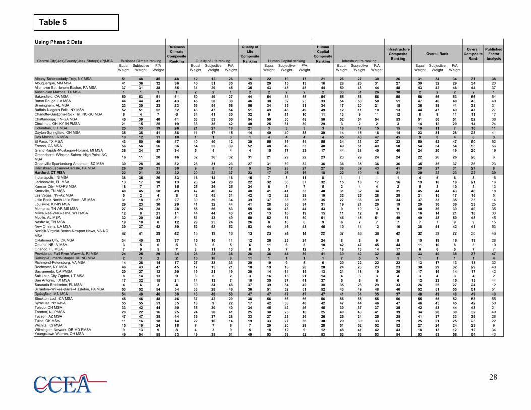
Table 5
Using Phase 2 Data
Central City(-ies)/County(-ies), State(s) (P)MSA
Business Climate
Composite Ranking
Quality of Life
Composite Ranking
Human Capital
Composite Ranking
Infrastructure Composite
Ranking
Overall Composite
Rank
Published Factor
Analysis
Equal Weight
Subjective Weight
F/A Weight
Equal Weight
Subjective Weight
F/A Weight
Equal Weight
Subjective Weight
F/A Weight
Equal Weight
Subjective Weight
F/A Weight
Equal Weight
Subjective Weight
F/A Weight
Albany-Schenectady-Troy, NY MSA 51 48 45 48 12 12 26 16 22 19 17 21 26 27 30 26 31 34 34 31 38Albuquerque, NM MSA 41 36 32 36 46 51 35 45 20 15 13 16 28 26 31 27 39 32 29 34 20Allentown-Bethlehem-Easton, PA MSA 37 31 38 35 31 29 45 35 43 45 45 44 50 48 44 48 43 42 46 44 37Austin-San Marcos, TX MSA 1 1 1 1 2 2 1 2 2 2 2 2 33 31 26 30 2 2 2 2 1Bakersfield, CA MSA 50 53 51 51 50 49 27 44 54 54 55 54 55 56 56 55 56 56 53 56 54Baton Rouge, LA MSA 44 44 43 43 45 50 38 46 38 32 25 33 54 50 50 51 47 46 40 45 40Birmingham, AL MSA 23 30 23 23 56 54 56 56 34 35 31 34 17 20 21 18 36 38 41 38 31Buffalo-Niagara Falls, NY MSA 52 51 52 52 48 47 54 51 49 48 49 49 12 11 10 13 44 47 49 47 27Charlotte-Gastonia-Rock Hill, NC-SC MSA 6 4 7 6 34 41 30 32 9 11 10 11 13 9 11 12 8 9 11 11 17Chattanooga, TN-GA MSA 40 39 40 41 53 53 55 54 50 50 48 50 52 54 54 53 51 50 51 52 36Cincinnati, OH-KY-IN PMSA 21 15 25 19 38 35 42 40 25 31 30 29 3 2 2 3 14 12 20 14 24Columbus, OH MSA 25 33 19 26 21 27 18 21 3 3 3 3 16 17 15 15 10 11 7 10 11Dayton-Springfield, OH MSA 35 38 41 38 11 17 15 14 40 40 38 39 14 15 16 14 23 31 28 28 41Des Moines, IA MSA 10 12 11 10 1 1 3 1 4 4 4 4 45 43 47 45 9 8 4 6 3El Paso, TX MSA 43 50 49 47 40 40 12 30 55 55 54 55 34 33 27 32 50 52 47 50 52Fresno, CA MSA 56 56 56 56 54 55 39 52 48 49 53 48 49 51 49 50 54 54 54 55 56Grand Rapids-Muskegon-Holland, MI MSA 36 34 37 34 5 4 4 4 15 17 23 17 44 38 40 40 24 20 19 20 19Greensboro--Winston-Salem--High Point, NC MSA 16 11 20 16 32 36 32 31 21 29 22 23 23 29 24 24 22 26 26 26 6
Greenville-Spartanburg-Anderson, SC MSA 30 28 36 32 28 31 23 27 31 39 32 36 36 35 36 36 35 35 37 36 23Harrisburg-Lebanon-Carlisle, PA MSA 26 29 31 30 9 8 17 9 24 28 27 27 38 39 43 41 28 27 31 27 8Hartford, CT MSA 22 21 22 22 20 22 37 23 17 26 16 18 22 19 18 21 20 22 23 22 39Indianapolis, IN MSA 38 35 26 33 16 14 16 15 7 8 11 8 1 1 1 1 4 5 6 3 16Jacksonville, FL MSA 13 17 10 13 23 24 20 22 32 30 37 32 15 16 17 16 19 18 18 21 16Kansas City, MO-KS MSA 18 7 17 15 25 26 25 24 6 5 7 5 2 4 4 2 5 3 10 5 13Knoxville, TN MSA 48 45 50 49 47 46 47 48 41 41 33 40 31 32 34 31 45 44 43 46 18Las Vegas, NV-AZ MSA 5 2 4 3 42 45 31 42 12 22 28 19 32 25 28 28 21 15 17 16 5Little Rock-North Little Rock, AR MSA 31 18 27 27 39 39 34 39 37 33 35 35 27 36 39 34 37 33 35 35 14Louisville, KY-IN MSA 29 23 30 29 41 32 44 41 28 36 34 31 19 21 20 19 29 30 36 33 25Memphis, TN-AR-MS MSA 27 24 28 28 55 56 53 55 46 43 44 43 9 10 13 9 40 36 39 40 35Milwaukee-Waukesha, WI PMSA 12 8 21 11 44 44 43 43 13 16 19 15 11 12 8 11 16 14 21 18 33Mobile, AL MSA 32 20 34 31 51 43 49 50 52 51 50 51 46 45 51 49 49 48 50 48 45Nashville, TN MSA 19 10 8 12 29 25 24 26 8 10 6 9 6 7 7 7 7 7 9 9 15New Orleans, LA MSA 39 37 42 39 52 52 52 53 44 46 43 46 10 14 12 10 38 41 42 41 53Norfolk-Virginia Beach-Newport News, VA-NC MSA 42 41 39 42 13 19 10 13 23 24 14 22 37 46 38 42 32 39 22 30 46
Oklahoma City, OK MSA 34 40 33 37 15 10 11 12 26 25 24 24 8 8 9 8 15 19 16 19 28Omaha, NE-IA MSA 3 5 6 5 6 5 5 6 11 6 8 10 42 47 45 44 11 10 8 8 10Orlando, FL MSA 7 9 5 7 8 11 13 8 5 7 12 7 18 13 14 17 6 6 5 7 7Providence-Fall River-Warwick, RI MSA 24 25 29 24 26 23 36 28 36 44 39 41 39 42 32 38 33 40 38 37 47Raleigh-Durham-Chapel Hill, NC MSA 2 3 2 2 10 18 8 11 1 1 1 1 7 5 5 5 1 1 1 1 4Richmond-Petersburg, VA MSA 14 26 14 17 27 33 33 29 10 9 5 6 20 22 22 22 13 17 13 13 32Rochester, NY MSA 46 43 47 45 17 15 21 18 19 18 20 20 24 23 23 23 30 29 32 29 40Sacramento, CA PMSA 20 27 12 20 19 21 19 20 14 14 15 13 21 18 19 20 17 16 14 17 42Salt Lake City-Ogden, UT MSA 8 14 13 9 3 6 2 3 16 13 21 14 4 3 3 4 3 4 3 4 2San Antonio, TX MSA 17 32 15 21 14 13 7 10 35 37 41 37 5 6 6 6 12 23 15 15 44Sarasota-Bradenton, FL MSA 4 6 3 4 30 34 48 37 39 34 42 38 35 28 29 33 26 25 27 24 12Scranton--Wilkes-Barre--Hazleton, PA MSA 53 52 54 54 33 28 46 36 51 52 51 52 43 49 48 46 52 51 55 51 51Springfield, MA MSA 54 49 46 50 43 48 50 47 47 47 47 47 41 34 35 37 48 49 48 49 48Stockton-Lodi, CA MSA 45 46 48 46 37 42 29 38 56 56 56 56 56 55 55 56 55 55 52 53 55Syracuse, NY MSA 55 55 53 55 18 9 22 17 42 38 40 42 47 44 46 47 46 45 45 42 50Toledo, OH MSA 33 42 44 40 35 30 40 34 45 42 46 45 30 37 37 35 42 43 44 43 21Trenton, NJ PMSA 28 22 16 25 24 20 41 25 30 23 18 25 40 40 41 39 34 28 30 32 49Tucson, AZ MSA 47 47 35 44 36 37 28 33 27 21 26 26 25 24 25 25 41 37 33 39 26Tulsa, OK MSA 11 16 18 14 22 16 14 19 33 27 36 30 29 30 33 29 25 21 25 25 22Wichita, KS MSA 15 19 24 18 7 7 6 7 29 20 29 28 51 52 52 52 27 24 24 23 9Wilmington-Newark, DE-MD PMSA 9 13 9 8 4 3 9 5 18 12 9 12 48 41 42 43 18 13 12 12 34Youngstown-Warren, OH MSA 49 54 55 53 49 38 51 49 53 53 52 53 53 53 53 54 53 53 56 54 43
Overall Rank
Business Climate ranking Quality of Life ranking Human Capital ranking Infrastructure ranking
28

Table 6
Using Phase 1 data
Central City(-ies)/County(-ies), State(s) (P)MSA
Business Climate
Composite Ranking
Quality of Life Composite
Ranking
Human Capital
Composite Ranking
Infrastructure Composite
Ranking
Overall Composite
Rank
Published Factor
Analysis
Equal Weight
Subjective Weight
F/A Weight
Equal Weight
Subjective Weight
F/A Weight
Equal Weight
Subjective Weight
F/A Weight
Equal Weight
Subjective Weight
F/A Weight
Equal Weight
Subjective Weight
F/A Weight
Albany-Schenectady-Troy, NY MSA 50 51 46 50 27 17 40 27 19 18 17 18 19 17 24 19 30 25 30 27 38Albuquerque, NM MSA 33 38 21 28 32 47 17 34 20 15 20 20 16 15 10 14 22 23 13 24 20Allentown-Bethlehem-Easton, PA MSA 41 40 43 41 31 18 44 31 46 47 45 47 32 31 27 31 42 42 44 44 37Austin-San Marcos, TX MSA 23 27 6 21 3 7 2 4 1 1 1 1 42 32 38 37 3 3 2 2 1Bakersfield, CA MSA 56 56 56 56 46 51 23 46 54 54 54 54 54 55 56 54 55 56 55 56 54Baton Rouge, LA MSA 29 31 33 30 33 45 35 40 40 33 29 37 41 38 40 41 39 39 37 40 40Birmingham, AL MSA 27 23 31 26 55 55 56 55 43 43 41 43 9 20 20 16 41 41 45 43 31Buffalo-Niagara Falls, NY MSA 47 44 48 48 45 38 52 48 44 45 47 45 27 21 21 24 48 45 48 47 27Charlotte-Gastonia-Rock Hill, NC-SC MSA 10 10 8 9 44 41 38 45 11 13 11 11 30 24 30 29 15 13 17 15 17Chattanooga, TN-GA MSA 34 30 35 32 54 46 54 54 52 52 50 52 36 45 41 40 53 51 51 53 36Cincinnati, OH-KY-IN PMSA 11 9 17 11 38 34 39 35 25 29 25 26 15 6 11 12 17 17 28 20 24Columbus, OH MSA 25 28 22 25 24 26 19 23 5 4 4 4 31 29 34 32 11 10 7 10 11Dayton-Springfield, OH MSA 35 32 40 36 13 16 12 13 42 42 39 42 14 11 13 13 27 29 32 30 41Des Moines, IA MSA 5 4 7 4 5 2 5 5 3 3 3 3 25 27 26 27 2 2 3 3 3El Paso, TX MSA 43 45 52 45 12 32 8 12 55 55 55 55 39 35 33 35 49 53 47 48 52Fresno, CA MSA 52 54 53 53 47 53 25 47 49 50 53 50 53 52 54 53 54 54 53 54 56Grand Rapids-Muskegon-Holland, MI MSA 14 15 23 15 2 1 4 2 14 17 18 14 56 54 55 56 18 18 14 11 19Greensboro--Winston-Salem--High Point, NC MSA 7 7 13 8 37 31 33 33 16 24 19 19 48 51 51 50 24 24 25 21 6Greenville-Spartanburg-Anderson, SC MSA 4 5 18 7 51 44 43 50 29 37 26 33 51 49 50 51 37 36 39 35 23Harrisburg-Lebanon-Carlisle, PA MSA 22 24 20 23 9 5 18 9 15 19 15 17 29 33 31 30 13 15 15 14 8Hartford, CT MSA 12 16 10 12 14 21 30 19 38 38 42 40 11 10 6 9 16 22 26 23 39Indianapolis, IN MSA 16 18 11 16 20 11 20 18 12 11 13 12 2 2 4 3 7 7 9 8 16Jacksonville, FL MSA 38 41 27 35 41 39 45 41 30 30 36 32 24 22 25 23 36 34 38 38 16Kansas City, MO-KS MSA 17 13 12 14 28 20 31 26 6 5 6 6 6 9 15 7 6 5 8 7 13Knoxville, TN MSA 42 42 45 43 52 50 51 51 31 32 27 31 33 37 35 33 46 44 43 46 18Las Vegas, NV-AZ MSA 3 2 3 3 48 42 32 44 27 31 38 29 50 47 48 48 33 28 23 25 5Little Rock-North Little Rock, AR MSA 28 25 26 27 49 48 46 49 22 22 21 21 18 30 22 21 28 30 27 29 14Louisville, KY-IN MSA 20 14 28 20 43 36 41 42 34 36 33 34 23 26 28 26 31 31 35 34 25Memphis, TN-AR-MS MSA 24 22 25 24 56 56 55 56 47 46 46 46 8 13 14 10 45 46 46 45 35Milwaukee-Waukesha, WI PMSA 8 11 14 10 34 35 28 32 9 9 9 9 22 14 16 18 9 9 10 9 33Mobile, AL MSA 31 33 32 29 53 52 50 52 51 51 51 51 35 42 39 39 50 52 49 50 45Nashville, TN MSA 39 36 19 33 42 40 42 43 10 10 10 10 1 3 3 1 10 14 12 12 15New Orleans, LA MSA 32 37 44 38 50 54 53 53 50 49 49 49 12 16 19 15 44 48 50 49 53Norfolk-Virginia Beach-Newport News, VA-NC MSA 49 49 47 51 8 15 9 8 36 34 37 36 52 53 52 52 47 47 36 39 46Oklahoma City, OK MSA 37 35 34 37 21 22 21 22 24 25 23 23 5 8 9 6 19 21 21 22 28Omaha, NE-IA MSA 6 6 5 5 4 4 3 3 8 6 5 7 34 44 36 38 5 6 5 5 10Orlando, FL MSA 9 8 4 6 10 14 15 11 4 8 8 5 47 40 45 46 8 8 6 6 7Providence-Fall River-Warwick, RI MSA 13 20 24 18 30 30 37 30 39 39 43 41 37 39 32 34 32 35 40 36 46Raleigh-Durham-Chapel Hill, NC MSA 1 1 1 1 25 25 11 20 2 2 2 2 3 1 1 2 1 1 1 1 4Richmond-Petersburg, VA MSA 15 17 9 13 26 24 26 24 17 16 14 15 21 25 29 25 14 16 11 16 48Rochester, NY MSA 40 39 41 40 15 8 27 15 13 12 12 13 43 36 42 42 25 19 24 19 40Sacramento, CA PMSA 48 53 37 46 17 29 10 17 21 20 28 22 46 41 46 45 38 38 31 37 42Salt Lake City-Ogden, UT MSA 18 21 16 19 1 3 1 1 7 7 7 8 10 4 5 8 4 4 4 4 2San Antonio, TX MSA 45 47 39 44 7 23 7 7 32 40 40 38 7 7 8 5 23 37 22 28 44Sarasota-Bradenton, FL MSA 2 3 2 2 35 33 49 37 23 23 32 25 26 19 12 20 12 12 18 13 12Scranton--Wilkes-Barre--Hazleton, PA MSA 55 52 55 54 23 13 36 25 48 48 48 48 45 48 47 47 51 49 52 51 51Springfield, MA MSA 53 50 50 52 19 37 34 28 45 44 44 44 13 12 7 11 40 43 41 41 48Stockton-Lodi, CA MSA 54 55 54 55 36 49 24 36 56 56 56 56 55 56 53 55 56 55 56 55 55Syracuse, NY MSA 46 46 51 49 22 12 29 21 37 35 34 35 44 43 44 44 43 40 42 42 50Toledo, OH MSA 26 26 42 31 11 9 16 10 41 41 35 39 20 28 23 22 26 33 34 31 21Trenton, NJ PMSA 44 43 30 42 39 28 48 39 35 27 24 28 4 5 2 4 35 26 29 32 49Tucson, AZ MSA 51 48 36 47 29 43 22 29 18 14 16 16 17 18 17 17 29 27 19 26 26Tulsa, OK MSA 36 29 38 34 16 19 13 16 33 28 30 30 38 34 37 36 34 32 33 33 22Wichita, KS MSA 21 19 29 22 6 6 6 6 28 26 31 27 40 46 43 43 21 20 20 18 9Wilmington-Newark, DE-MD PMSA 19 12 15 17 18 10 14 14 26 21 22 24 28 23 18 28 20 11 16 17 34Youngstown-Warren, OH MSA 30 34 49 39 40 27 47 38 53 53 52 53 49 50 49 49 52 50 54 52 43
Overall Rank
Business Climate Ranking Quality of Life Ranking Human Capital Ranking Infrastructure Ranking
29

Conclusion MetroHartford has apparently fallen behind some of its competitors over the last few
years according to the metric established to assess its performance. This is accountable
by its later recovery from the early 90s recession, its paucity of development projects
relative to other areas (see the comparative cities report cited above) in the middle 90s,
and, the lag of the effects of (local) policy and institutional changes. It is essential that
local changes be recorded and described such that they can be tracked via the benchmark
process. There are lags as well in the effects of economic development, policy and
institutional changes as they manifest in the benchmark variables we assemble (some
variables are annual, others biannual, quadrennial, and some, decennial).
Future Work
The linear methods employed here are not as good as they get. There is much benchmark
work proceeding using dynamic factor analysis (BEA is researching these methods for
various indicators). This time series technique offers the ostensibly unbiased approach of
statistical correlation (weighting) and stability over time because changes in variables are
conditioned on their history. We are researching dynamic factor analysis as a viable
alternative to the linear methods and expect to produce the next benchmark using both.
30

Appendix 1:
First Annual Report: The MetroHartford Benchmarking Project
31

F
THE METROHA
ConnectiConnecti
U
IRST ANNUAL REPORT —
RTFORD BENCHMARKING PROJECT©
by
Thomas J. Cooke Fred Carstensen
William Lott Stan McMillen
Joel Corona Hulya Varol
cut Metropolitan Studies Initiative cut Center for Economic Analysis
niversity of Connecticut
January 12, 1999

EXECUTIVE SUMMARY This report from the Connecticut Metropolitan Studies Initiative of the Connecticut Center for Economic Analyisis, University of Connecticut presents a series of indices and rankings comparing the MetroHartford metropolitan area with 56 similar metropolitan areas throughout the United States. We emphasize that the analysis is based upon the Metropolitan Statistical Area (MSA) as the unit of analysis because the MSA is a federal standard for the comparison of urban areas. The indices and rankings are designed to serve as benchmarks for the MetroHartford Millennium Project in three ways: 1) to evaluate the efficacy of current policy by comparing changes in MetroHartford’s ranking over time, 2) to explain MetroHartford’s current competitive standing by comparing MetroHartford’s ranking to competitors, and 3) to identify effective economic development policies by examining the policies of the top-ranked metropolitan areas. The analysis identified three factors - Economic Vitality, Quality of Life, Socio-Economic Productivity - and a Summary Index which describe the performance of metropolitan areas.
None of the top six metropolitan areas are in the Rust Belt.
Among the nineteen Rust Belt metropolitan areas, twelve, including MetroHartford, are in the bottom half.
MetroHartford Ranks 54th out of 56 comparable metropolitan areas in terms of Economic Vitality.
MetroHartford Ranks 4th out of 56 comparable metropolitan areas in terms of Quality of Life.
MetroHartford Ranks 39th out of 56 comparable metropolitan areas in terms of Socio-Economic Productivity.
MetroHartford Ranks 39th out of 56 comparable metropolitan areas in terms of the Summary Index.
The results do not indicate causal relationships, rather they indicate correlations. The results thus suggest and support certain policy initiatives where MetroHartford is ranked relatively low. For example, across all MSA’s Economic Vitality is inversely related to corporate income tax burden, and positively related to manufacturing employment growth, and Quality of Life is inversely related to
-i-

violent crime, and positively related to educational attainment. To improve the current analysis, we should extend the benchmark from the early 1980s to the present to place current efforts in their historic context. The exercise described here should be replicated annually as new data become available and as the Project begins to bear fruit. Future work should have separate components, which focus on just the metropolitan areas of New England, and, because metropolitan area variables mask the characteristics of cities and towns, we should replicate this analysis for the core cities, and their components, of the New England region. There are other variables to add that may improve the focus for policy, and, we should include all 360 MSA’s to improve the resolution of MetroHartford’s position nationally.
-ii-

INTRODUCTION
This report from the Connecticut Metropolitan Studies Initiative of the Connecticut Center
for Economic Analysis, University of Connecticut presents a series of indices and rankings
comparing the MetroHartford metropolitan area to similar metropolitan areas throughout the United
States. These indices and rankings are designed to serve as benchmarks for the MetroHartford
economic development community in three ways: 1) to evaluate the efficacy of current policy by
comparing changes in MetroHartford’s ranking over time, 2) to explain MetroHartford’s current
competitive standing by comparing MetroHartford’s ranking to competitors, and 3) to identify
effective economic development policies by focusing on the policies of the top-ranked metropolitan
areas.
DATA AND METHODS
The objective of the analysis is to create a small number of indices, which reflect the
multiple ways in which metropolitan areas differ from each other. This objective was articulated
through extensive meetings with the Economic Advisory Board of the MetroHartford Millennium
Project.1 The advisory board first identified that the units of analysis should be metropolitan
statistical areas (MSA). MSAs consist of large core cities together with adjacent communities that
have a high degree of economic and social integration with that core. The MSA classification is a
statistical standard, developed for use by Federal agencies in the production, analysis, and
publication of data on urban areas. The Economic Advisory Board then identified a set of
1Jeffrey Blodgett, Connecticut Economic Resource Center; Fred Carstensen, University of Connecticut/CCEA; Thomas Cooke, University of Connecticut/CMSI/CCEA; Stan McMillen, University of Connecticut/CCEA; Michael Levin, Connecticut Light & Power; William Lott, University of Connecticut/CCEA; James Moor, The Hartford Financial Services Group; John
-1-
metropolitan areas comparable to MetroHartford in terms of spatial structure, population, economic
structure, and region:
The first screen excluded all Primary Statistical Metropolitan Areas (PMSAs) (these are metropolitan areas that are part of larger urban agglomerations);
The second screen excluded all metropolitan areas with a population less than 500,000 or
greater than 1,500,000;
The third screen added back several PMSAs between 500,000 and 1,500,000, which are comparable to MetroHartford but were not selected in the first two screens: Trenton, NJ; New Haven, CT; Milwaukee, WI; Sacramento, CA; Cincinnati, OH;
The final screen added MSAs and PMSAs either less than 500,000 or greater than 1,500,000
that were judged important for comparison: Bridgeport, CT; Norfolk, VA; Kansas City, MO. Table 1 lists each of these metropolitan areas and their 1996 population.
To identify indices for ranking these metropolitan areas the Economic Advisory Board
identified four broad criteria to guide data collection: 1) Business Climate, 2) Human Capital, 3)
Quality of Life, and 4) Infrastructure. For each of these criteria, the Economic Advisory Board
identified a set of variables considered to reflect various dimensions of the four criteria. Table 2
lists these criteria and the selected variables. The selection of these variables was further based on
the following criteria:
♦ The data must be available for all of the selected metropolitan areas;2 ♦ Newer data is preferred over older data; ♦ Updates should be available frequently; ♦ Projected data should be excluded; ♦ Data reported at the metropolitan level is preferred over city, county, or state data; ♦ Included data are supported by economic or sociological theory. Shemo, Connecticut Capitol Region Growth Council.
2There were a few cases in which data for specific variables were missing for specific metropolitan areas. Various methods were used to impute the missing data. In the case of Bridgeport and New Haven, the large amount of missing data meant that they were ultimately excluded from the study even though they were selected to be part of the study. This occurred because much of the US Census data for Bridgeport and New Haven are rolled together with data for the New York Consolidated Metropolitan Statistical Area.
-2-

The construction of any ranking system confronts the issue of how to combine these
variables to create useful measures.3 Our approach is to use factor analysis. Factor analysis is a
traditional multivariate statistical method for reducing a large number of correlated variables to a
small number of independent indices (or factors).4 The resulting analysis of the selected data
identified three factors - Economic Vitality, Quality of Life, Socio-Economic Productivity.5 These
three factors were also used to construct a Summary Index.
RESULTS
Table 3 lists each of the three factors extracted from the data and those variables which are
most highly correlated with each factor. Table 4 lists the index scores for each factor in two ways:
1) as a ranking, and 2) as a probability level. Table 4 is sorted according to a Summary Index
which is a function of the three factors (see below).
Economic Vitality. The first factor - Economic Vitality - is most highly correlated with growth in
key industries, growth in income, growth in population, number of housing starts, and corporate tax
3Guterbock, T.M. 1997. Why Money Magazine’s “Best Places” keep changing. Public Opinion Quarterly, 61:339-351;
Nissan, E. 1994. A composite index for statistical inference for ranking metropolitan areas. Growth and Change, 25(4):411-427;
Shresha, H., and C. McCue. 1998. Measuring Performance of Metropolitan Areas in the US: A Literature Survey. Storrs, CT: Center for Economic Analysis, University of Connecticut.
4Technically, we use a scree plot from principal factor analysis to extract 5 factors from the data. We then use unweighted least squares factor analysis with a varimax rotation. The 2 smallest factors were not meaningful, thus leaving 3 factors.
5The three factors explain 71% of the variation in the variables across the included metropolitan areas.
-3-

burdens. Metropolitan areas with a high Economic Vitality score are metropolitan areas with
vibrant, expanding economies, good business climates, and high rates of immigration from other
parts of the country. As expected given the economic troubles of the early 1990s, relative to the
other metropolitan areas in the study, MetroHartford ranks 54th out of 56 which places it in the 4th
percentile. In other words, only 4% of metropolitan areas can be expected to score lower in terms
of Economic Vitality than MetroHartford.
Quality of Life. The second factor - Quality of Life - is most highly correlated with income levels,
poverty rates, crime rates, climate, family structure, and educational attainment. Metropolitan areas
with a high Quality of Life score have high incomes, low poverty, low crime, temperate climates,
and high education levels. Indeed, such a description aptly applies to MetroHartford. Relative to
the other metropolitan areas in the study, MetroHartford ranks 4th out of 56 which places it in the
93rd percentile. In other words, fully 93% of metropolitan areas can be expected to fare worse in
terms of Quality of Life than MetroHartford.
Socio-Economic Productivity. The third factor - Socio-Economic Productivity - is most highly
correlated with economic output per capita, personal bankruptcy rates, unemployment rates, quality
of physical infrastructure, educational attainment, and, social dependence. Metropolitan areas with
a high Socio-Economic Productivity score are those in which the economic and social infrastructure
results in high rates of economic activity and productive industries. Relative to the other
metropolitan areas in the study, MetroHartford ranks 39th out of 56, which places it in the 38th
percentile. In other words, only 38% of metropolitan areas can be expected to fare worse in terms
of Socio-Economic Productivity.
-4-

Summary Index. The three individual indices are combined into a Summary Index by weighting
the three factor scores by the percent of the total variance attributed to that factor. Thus, the
summary factor scores give an overall rank and percentile score which largely reflects Economic
Vitality (37% of the total), followed by Quality of Life (36% of the total), and Socio-Economic
Productivity (27% of the total). As expected given the range of scores on the three individual
indices, MetroHartford is in the middle of the pack. Overall, MetroHartford ranks 39th out of 56,
which places it in the 41st percentile.
Regional Patterns. The Summary Index indicates six metropolitan areas which rank significantly
higher than the remaining metropolitan areas (Austin, TX; Salt Lake City, UT; Des Moines, IA;
Raleigh, NC; Las Vegas, NV; Greensboro, NC). None of these metropolitan areas are within the
Rust Belt (Rust Belt metropolitan areas are underlined in Table 4). Economic Vitality and Quality
of Life are significantly higher in this group. Among the nineteen Rust Belt metropolitan areas,
twelve, including Hartford, are in the bottom half of the sample with respect to the Summary Index.
Comparison with Other New England Metropolitan Areas. Only two other New England
metropolitan areas were included in the analysis: Providence, RI and Springfield, MA. Overall,
Providence and Springfield fare significantly worse than MetroHartford. Both Providence and
Springfield are similar to MetroHartford in terms of Economic Vitality (51st, 52nd, and 54th
respectively) and Socio-Economic Productivity (30th, 42nd, and 39th respectively), but
MetroHartford is much better off in terms of Quality of Life (25th, 20th, and 4th respectively). The
higher Quality of Life boosts MetroHartford’s Summary Index to 39th, in comparison to Providence
-5-

(47th) and Springfield (48th).
CONCLUSIONS
This analysis provides the MetroHartford Millennium Management Committee with a broad
set of indices upon which to evaluate past and future economic development policy. In particular,
MetroHartford’s high Quality of Life is overshadowed by its low Economic Vitality and marginal
Socio-Economic Productivity.
There are several ways that these results can be used. First, the results can be used to
explain MetroHartford’s current standing by comparing MetroHartford’s ranking to competitors.
Second, the results can be used to identify effective economic development policies by examining
the policies of the top-ranked metropolitan areas. A third use for the results is to evaluate the
efficacy of current policy by comparing changes in MetroHartford’s ranking over time. The current
results do not now allow such an analysis because they are limited to data from the early- to mid-
1990s, but this will be addressed in subsequent work (see below). Fourth, while the results do not
indicate causal relationships - rather they indicate correlations - the results suggest and support
certain policy initiatives where MetroHartford is ranked relatively low. For example, across all
MSA’s Economic Vitality is inversely related to corporate income tax burden, and positively related
to manufacturing employment growth, and Quality of Life is inversely related to violent crime, and
positively related to educational attainment.
FUTURE WORK
To make the benchmark project truly valuable, however, it must be sustained and enriched.
What we now have is a single snapshot of MetroHartford’s competitive position. But we do not
-6-

know how MetroHartford’s performance has evolved over time, nor how it compared with other
regions five, ten or fifteen years ago. To improve the current analysis we should extend the
benchmark from the early 1980s to the present to place current efforts in their historic context. And
even though we have considered over 100 data series in building the analysis, there are other
relevant series that need to be evaluated, there are important variables (e.g., the availability of local
venture capital) which have not yet been included because usable data is not directly available and
must be constructed or inferred from other data series. There are important regions with which we
should compare MetroHartford (principally similar MSA’s in the Northeast), but for which
appropriate data was not available. The exercise described here should be replicated annually as
new data become available and as the Project begins to bear fruit. Because metropolitan variables
mask the characteristics of cities and towns, we should replicate this analysis for the core cities, and
their components, of the New England region.
-7-

Table 1. Metropolitan Areas Population (1996).
Metropolitan area Pop.
(000s) Metropolitan area Pop.
(000s)Albany-Schenectady-Troy, NY 878 Memphis, TN-AR-MS 1,078
Albuquerque, NM 670 Milwaukee-Waukesha , WI 1,457Allentown-Bethlehem-Easton, PA 614 Mobile, AL 518Austin-San Marcos, TX 1,041 Nashville, TN 1,117Bakersfield, CA 622 New Orleans, LA 1,312Baton Rouge, LA 567 Norfolk-Virginia Beach, VA 1,540Birmingham, AL 894 Oklahoma City, OK 1,026Buffalo-Niagara Falls, NY 1,175 Omaha, NE-IA 681Charlotte-Gastonia-Rock Hill, NC-SC 1,321 Orlando, FL 1,417Chattanooga, TN-GA 446 Providence-Fall River, RI-MA 1,124Cincinnati , OH-KY-IN 1,597 Raleigh-Durham-Chapel Hill, NC 1,025Columbus, OH 1,447 Richmond-Petersburg, VA 935Dayton-Springfield, OH 950 Rochester, NY 1,088 Des Moines, IA 427 Sacramento , CA 1,482El Paso, TX 684 Salt Lake City-Ogden, UT 1,217Fresno, CA 861 San Antonio, TX 1,490Grand Rapids-Muskegon-Holland, MI 1,015 Sarasota-Bradenton, FL 528Greensboro--Winston-Salem, NC 1,141 Scranton—Wilkes Barre—Hazelton, PA 628Greenville-Spartanburg-Anderson, SC 896 Springfield, MA 576Harrisburg-Lebanon-Carlisle, PA 614 Stockton-Lodi, CA 533MetroHartford, CT 1,144 Syracuse, NY 745Indianapolis, IN 1,492 Toledo, OH 611Jacksonville, FL 1,008 Trenton , NJ 330Kansas City, MO-KS 1,690 Tucson, AZ 767Knoxville, TN 649 Tulsa, OK 756Las Vegas, NV-AZ 1,201 Wichita, KS 512Little Rock-North Little Rock, AR 548 Wilmington-Newark , DE-MD 550Louisville, KY-IN 991 Youngstown-Warren, OH 598
-8-

Table 2. Criteria and Variables.
Business Climate Quality of Life Government Share of Employment, 1996 % of Population below Poverty, 1993 Manufacturing Share of Employment, 1996 % of Families headed by Females, 1990 White Collar Share of Employment, 1996 Air Quality Index, 1997 State Corporate Income Tax Burden, 1993 Average Travel Time to Work, 1990 Bankruptcy Rate, 1995 Crude Death Rate, 1992-94 Economic Output per Capita, 1992 Crude Birth Rate, 1992-94 Construction Employment Growth, 1990-96 Heating and Cooling Degree Days,1997 Manufacturing Employment Growth, 1990-96 Housing Affordability Index, 1998 White Collar Employment Growth, 1990-96 Violent Crime Rate, 1997 Real Income per Capita, 1997 Motor Vehicle Death Rate, 1992 Real Income Growth per Capita, 1990-97 Single Family Home Price Growth, 1997 Housing Starts per Capita, 1997 Infrastructure Human Capital # of Hospital Beds per Capita, 1997 Total Population, 1997 FAA Airport Class (4=large, 1=no hub), 1997 Population Growth Rate, 1990-1997 Land Area, 1990 Dependent Population Ratio, 1996 Number of Interstate Highways, 1997 Economic Activity Rate, 1996 Patents & Innovations Per Capita, 1996 Labor Force Participation Rate, 1996 Physicians per Capita, 1993 Unemployment Rate, 1996 Population Density, 1990/1997 % Foreign Born, 1990 % with Diploma or GED, 1990 % with College Degree, 1990
-9-
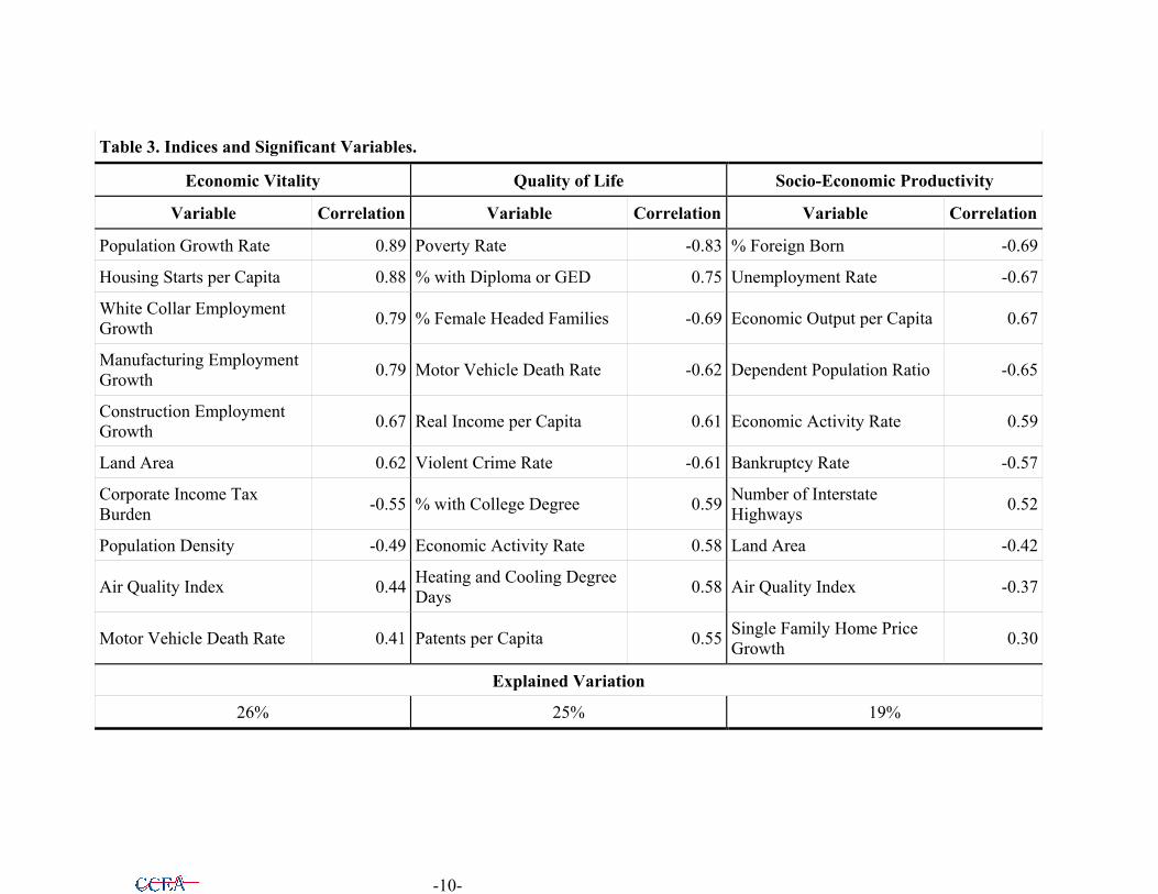
Table 3. Indices and Significant Variables.
Economic Vitality Quality of Life Socio-Economic Productivity
Variable Correlation Variable Correlation Variable Correlation
Population Growth Rate 0.89 Poverty Rate -0.83 % Foreign Born -0.69
Housing Starts per Capita 0.88 % with Diploma or GED 0.75 Unemployment Rate -0.67
White Collar Employment Growth 0.79 % Female Headed Families -0.69 Economic Output per Capita 0.67
Manufacturing Employment Growth 0.79 Motor Vehicle Death Rate -0.62 Dependent Population Ratio -0.65
Construction Employment Growth 0.67 Real Income per Capita 0.61 Economic Activity Rate 0.59
Land Area 0.62 Violent Crime Rate -0.61 Bankruptcy Rate -0.57
Corporate Income Tax Burden -0.55 % with College Degree 0.59 Number of Interstate
Highways 0.52
Population Density -0.49 Economic Activity Rate 0.58 Land Area -0.42
Air Quality Index 0.44 Heating and Cooling Degree Days 0.58 Air Quality Index -0.37
Motor Vehicle Death Rate 0.41 Patents per Capita 0.55 Single Family Home Price Growth 0.30
Explained Variation
26% 25% 19%
-10-

Table 4. Index Scores and Rankings Sorted by Summary Index.
Summary Index
Economic Vitality
Quality of Life
Socio-Economic
ProductivityMSA Rank Score Rank Score Rank Score Rank Score
Austin-San Marcos, TX 1 94 2 99 5 92 17 75 Salt Lake City-Ogden, UT 2 89 5 89 2 96 20 73 Des Moines, IA 3 86 9 83 1 96 28 61 Raleigh-Durham-Chapel Hill, NC 4 84 4 92 13 79 18 74 Las Vegas, NV-AZ 5 83 1 100 16 72 56 0 Greensboro--Winston-Salem, NC 6 82 6 88 23 60 3 92 Orlando, FL 7 72 3 95 24 58 41 36 Harrisburg-Lebanon-Carlisle, PA 8 71 37 40 9 85 7 84 Wichita, KS 9 68 12 79 17 71 34 47 Omaha, NE-IA 10 68 41 28 7 88 6 84 Columbus, OH 11 66 30 48 12 81 24 65 Sarasota-Bradenton, FL 12 64 7 88 19 67 45 20 Kansas City, MO-KS 13 63 31 48 22 65 14 78 Little Rock-North Little Rock, AR 14 61 14 72 37 39 19 74Nashville, TN 15 61 15 71 39 37 16 76 Indianapolis, IN 16 60 35 44 27 53 5 84Charlotte-Gastonia-Rock Hill, NC-SC 17 59 24 55 42 29 2 92
Knoxville, TN 18 59 13 72 36 40 26 63 Grand Rapids, MI 19 58 36 43 15 75 31 53 Albuquerque, NM 20 57 11 79 26 54 44 27 Toledo, OH 21 57 33 45 31 48 10 81 Tulsa, OK 22 57 16 69 38 38 25 63 Greenville-Spartanburg-Anderson, SC 23 55 18 62 46 17 4 91
Cincinnati, OH-KY-IN 24 53 32 46 35 45 21 72 Louisville, KY-IN 25 53 26 52 41 30 11 81 Tucson, AZ 26 53 8 85 32 47 47 14 Buffalo-Niagara Falls, NY 27 52 21 58 34 47 32 50 Oklahoma City, OK 28 51 38 38 40 37 8 84
-11-

Table 4 continued
Summary Index
Economic Vitality
Quality of Life
Socio-Economic
Productivity MSA Rank Score Rank Score Rank Score Rank Score
Jacksonville, FL 29 50 10 80 43 25 36 41 Rochester, NY 30 49 50 8 3 95 37 40 Birmingham, AL 31 49 17 68 45 20 22 66 Richmond-Petersburg, VA 32 48 39 36 29 51 29 60 Milwaukee-Waukesha, WI 33 48 46 21 18 67 27 62 Wilmington-Newark, DE-MD 34 47 47 19 11 83 38 39 Memphis, TN-AR-MS 35 46 19 60 52 5 1 94 Chattanooga, TN-GA 36 45 25 52 48 14 9 82 Allentown-Bethlehem-Easton, PA 37 45 45 23 10 84 46 20 Albany-Schenectady-Troy, NY 38 42 44 23 8 87 50 11 MetroHartford, CT 39 41 54 3 4 93 39 38 Baton Rouge, LA 40 39 34 45 49 13 15 76 Dayton-Springfield, OH 41 39 49 8 28 51 13 80 Sacramento, CA 42 37 23 55 21 65 54 3 Youngstown-Warren, OH 43 37 29 49 44 23 35 42 San Antonio, TX 44 36 27 52 47 15 33 50 Mobile, AL 45 35 20 58 53 3 12 80 Norfolk-Virginia Beach-Newport News, VA 46 34 42 25 30 50 43 29
Providence-Fall River-Warwick, RI-MA 47 33 51 7 25 56 30 57
Springfield, MA 48 30 52 7 20 65 42 33 Trenton, NJ 49 30 55 3 6 91 48 13 Syracuse, NY 50 29 56 3 14 77 40 36 Scranton--Wilkes-Barre--Hazleton, PA 51 22 48 12 33 47 49 12
El Paso, TX 52 13 22 56 54 3 52 3 New Orleans, LA 53 12 53 5 55 3 23 66 Bakersfield, CA 54 12 28 50 50 9 55 0 Stockton-Lodi, CA 55 11 43 24 51 6 51 6 Fresno, CA 56 9 40 33 56 3 53 3
-12-

Appendix 2: Four Categories and Variables: Subjective Weighting Exercise

Millennium Benchmark Study In the following table you will find the 45 variables used to calculate the index in this study. In the first blank column, please rank these variables in a way that the most important variable to you is number 1, IRRESPECTIVE OF ITS CATEGORY. Then in the score column, please assign scores to these variables, where the most important variable gets the highest score. For scoring, you have 100 points to distribute among the variables in each category. You may use tick marks for each point you give to one variable, and the total score has to add up to 100 for each category. You may give the same score to different variables. The result establishes subjective weights for the variables in the analysis.
Category VARIABLES RANK SCORE
Infrastructure 100 points
1 City Land Area (sq. miles) 2 FAA Airport Classification6 3 Hospital Beds per 1000 pop. 4 No. of Interstate Highways 5 Metropolitan Land Area (MSA
sq. miles) 6 Patents per 1000 nonfarm
businesses 7 Physicians per 1000 pop. 8 Population Density
Total 100 Business Climate 100 points
1 Bankruptcy Rate 2 Construction Employment
Growth 3 Government Share of
Employment 4 Housing Start Rate 5 Manufacturing Employment
Growth 6 Real Gross State Product Per
Capita 7 Real Personal Income
Growth Per Capita 8 Real Personal Income Per
Capita
6 FAA's classification for the metro area: large=4, medium=3, small=2, and none=1.

9 State Corporate Income Tax Burden
10 White Collar Employment Growth
11 White Collar Share of Employment
12 Manufacturing Share of Employment
Total 100
Quality of Life 100 Points RANK SCORE
1 Heating & Cooling Degree Days
2 Housing Affordability Index 3 Birth Rate 4 Infant Mortality rate 5 Average Daily Commute
(round trip) 6 Death Rate 7 Voter Turnout (1996
presidential) 8 Motor Vehicle Death Rate 9 Particulate Matter
10 % of Female Headed Households
11 % of Population Below Poverty
12 Violent + Property Crimes per 1000 pop
13 Transfer Payments Per Capita
14 Single Family Home Price Growth
Total 100
Human Capital 100 Points
1 % of Population With Secondary Education
2 Adolescent Birth Rate 3 % of Population in 25 to 44
Cohort 4 Population Growth 5 1998 Population Level

6 Dependent Population Ratio (pop<16+pop>65/total pop)
7 Economically Active Population (16<=pop<65/total pop)
8 % of Population With Bachelors Degree
9 Unemployment Rate 10 Labor Force Participation
Rate 11 % of Foreign Born Population
Total 100
Now that you have scored the variables within each category, please score the categories. You have 100 points to assign among the four categories. Category Rank Points Infrastructure Business Climate Quality of Life Human Capital Total 100