NBER WORKING PAPER SERIES

TEMPORARY TERMS OF TRADE DISTURBANCES, THE REAL EXCHANGE RATE

AND THE CURRENT ACCOUNT

Sebastian Edwards

Working Paper No. 2629

NATIONAL BUREAU OF ECONOMIC RESEARCH 1050 Massachusetts Avenue

Cambridge, MA 02138 June 1988

A version of this paper was written while the author was visiting the Research Department of the International Monetary Fund. I want to thank

many colleagues at the Fund for providing an exciting atmosphere for under-

taking research on international economics. I have benefitted from discus- sions with Joshua Aizenman, Mohain Khan, Peter Montiel, Miguel Savastano and

Sweder van Wijnbergen. I am particularly grateful to two anonymous referees for very helpful suggestiona that greatly helped improve this paper. This research is part of NBER's research program in International Studies. Any opinions expressed are those of the author not those of the National Bureau of Economic Research.

NBER Working Paper #2629 June 1988

TEMPORARY TERMS OF TRADE DISTURBANCES, THE REAL EXCHANGE RATE

AND THE CURRENT ACCOUNT

ABSTRAct

In this paper a general equilibrium intertemporal model with optimizing

consumers and producera ia developed to analyze how the temporary term's of

trade diaturbances affect the path of real exchange rates and the current

account. Changes in the internal terms of trade (due to tariff changes) and

to the external terms of trade are considered. The model is completely

real, and considera a small open economy that produces and consumes three

goods each period. It is shown that, without imposing rigidities or adjust-

ment costs, interesting paths for the equilibrium real exchange rate can be

generated. In particular "equilibrium overshooting" can be observed:

Precise conditions under which a temporary import tariff will worsen the

current account in period 1 are derived. The way in which temporary and

permanent external terms of trade shocks will affect the current account are

analyzed. Several ways in which the model can be extended are discussed.

The results obtained from this model have important implications for the

design of balance of payments policy and for the analysis of real exchange

rate misalignrent and overvaluarion.

Sebastian Edwards

Department of Economics

University of California, Los Angeles

Los Angeles, CA 90024

(213) 825-5304

I. Introduction

The recent behavior of the external sector in a number of countries,

including the United States, has generated concern among policymakers and

academics. In fact, in the last few years policy analyses have increasingly

focused on issues related to the evolution of the trade and current

accounts, and some proposals aimed at altering some countries external posi-

tions have been intensively discussed. Perhaps one of the most hotly

debated policy measures consists of the imposition of (temporary) import

tariffs as a way of improving the internal terms of trade and, thus, a

I country's current account,

Historically, a number of countries have many times resorted to

protectionism as a means to face external payments difficulties; the imposi-

ti . of temporary impediments to trade -- in the form of import tariffs or

quotas, for example -- has in fact been a common prsctice aimed at improving

the current account and/or at changing the behavior of the real exchange

rate. In particular, this has been a very common feature of the Latin

American countries, which have recurrently tried to use temporary

protectionist measures as a way to influence the behavior of the external

sector. Many times, however, these protectionist policies hsve failed to

achieve their objectives, and in spite of increased levels of import tariffs

the current account balance has not experienced any improvements.2 Tradi-

tional trade theory has explained this phenomenon claiming that in some

cases the elasticities of demand for imports and exports can be very low.

These explanations, however, fail to recognize the fact that the current

account basically responds to intettempotal considerations, and that for any

policy measures to have an effect on its balance, it necessarily has to have

an impact on the country's savings and/or investment decisions,

The purpose of this paper is to develop s fully real optimizing

intertemporsl general equilibrium model to analyze how disturbances to terms

of trade - - both internal (due to tariff changes) and external - - affect the

current sccount. The analysis focuses on the cases of temporary import

tariffs and temporary external terms of trade shocks. In the Section IV,

however, the cases of permanent disturbances is also briefly discusaed. The

model considers a two-periods economy that produces and consumes three goods

-- exporrables, importablea and nonrradsbles. Consumers maximize intertemp-

oral utility, while producers maximize present value of profits. In this

three goods setting changes in the equilibrium real exchange rate - - or

equilibrium relative price of nontradables - - becomes a key intertemporal

channel through which the terms of trade disturbances impacr on the current

account. Although in recent years it has become customary to emphasize the

intertemporal nature of the current account, a large number of policy

discussions have in practice ignored this proposition and have proceeded

along the lines of traditional static textbook models. Also, a number of

applied papers have recently discussed the effects of tariffs on current

account behavior without acknowledging any interremporal factors. On the

other hand, many of the papers that have explicitly used an inttrtemporsl

setting have either used ad-hoc assumptions regarding consumers or

producers, or have only considered a two-goods world, being unable to deal

with the effects of import tariffs on the real exchange rare.3

II. The Model

In this section a real general equilibrium intertemporal model of a

small open economy is derived to analyze the way in which different

disturbances affect the current account. The model is based on Edwards

3

(1988c) and extends in several directions the intertemporal models of

Svenason and Razin (1983) and Edwards and van Wijnbergen (1986).

Conaider rhe case of a amall country that produces and conaumes three

goods - - importablea (N) , exporrables (X) and nontradablea (N) . There

are two periods - - the pcesent (period I) and the future (period 2)

Foreign borrowing and lending is allowed at the exogenoualy given world

interest rate r*. The country faces an intertemporal budget constraint

that atatea that the diacounted aum of the current account balances ia zero.

(Thiaa assumes that the initial debt commitment is zero.) There are a large

number of producers and (identical) consumers, and perfect competition

prevails. Consumers maximize utility subject to their intertemporal budget

constraint, whereas firma maxithize profits subject to existing technology

and availability of factora of production. In orc : to simplify the

exposition in the firat part of the paper it ia assumed that there ia no

investment. In Section V.2, however, investment is incorporated into the

analysis.

Assuming that the utility function ia time separahle, with each

subutility function homothetic and identical, the representative consumer

problem can be stated as follows:

max Q(u(cNcMcX); U(CNCMCXH.

subject to:

c + PcM + qc + &*(Cx+PCM+QCN)

S Wealth, (1)

where the lower case lettera refer to first period vatiablea and the upper

caae letters refer to second period variables. The price of the exportable

has been taken to be the numotaire (2 is the intertemporal welfare

function; u and U are periods l and 2 aubutility functions assumed, as

pointed out, to be homorhetic and identical. cx CM cN (Cx. CM and CN)

are consumption of K, H and N in period one (two). p and P are the

domestic prices of importable relative to exportablea in periods 1 and 2. q

and Q are prices of nontradables relative to exportahles in periods 1 and

2, and 5* is the world discount factor equal to (l+r*)1. It is assumed

that imports are subject to a tariff. Denoting periods 1 and 2 tariffs as

t and T, domestic prices of importables are related to world prices in

the following way (where an asterisk refers to a foreign variable):

p — p* + t; — '* + T (2)

Wealth is the discounted sum of consumer's income in both periods.

Income, in turn, is given in each period by three components: (1) income

from labor services rendered to firms; (2) income from the renting of

capital stock that consumers own to domestic firms; and (3) income obtain-

ed from government transfers. These, in turn, correspond to the proceeds

from import tariffs which the government hands back to the public. In this

model, then, as in most of the international trade literature, the govern-

ment plays no active role besides imposing import tariffa, and handing their

proceeds back to households in a nondiarortionary way.4

Given the nature of preferences, the consumer optimization process can

be thought of as taking place in two stages. First, the consumer decides

how to allocate his(her) wealth across periods. Second, he(she) decides how

to distribute each period (optimal) expenditure across the three goods. The

solution to the consumers optimizing problem is conveniently summarized by

the following intertemporal expenditure function:5

E — E(a(l,p,q), It(l,P,Q),Q}. (3)

where it and fl are exact price indexes for periods I and 2. Under the

5

assumptions of homotheticity and separability these price indexes correspond

to unit expenditure functions (Svensson and Razin, 1983) . A convenient

property of the expenditure function is that its derivative with respect to

each price is equal to the compensated demand curve for that good. For

instance, the compensat,d demand function for nontradables in period 1

(where a subindex refers to a partial derivative with respect to that vari-

able) is given by:

S —Em. q irq

Another important property of expenditure functions is that they are con-

cave. Moreover, given our assumption of a time separable utility function,

expenditure in periods I and 2 are substitutes. As a result, all intertemp-

oral cross demand effects are positive (i.e., E , E , E , S > pQ qP qQ pP

It is assumed that firms use conventional technology to produce N, X

and M. There are three factors of production - - capital, labor and natural

resources. Consequently, factor price equalization does not hold in either

period. At this point it is assumed that there is no investment, and that

all factor prices are fully flexible. Later, in Section V, however, both

assumptions will be relaxed. The producers' maximization problem can be

stated, in each period, in the following way (where v and V are vectors

of factors of production; w and are vectors of their rewards, and s.

and S. are outputs of good j in periods 1 and 2.)

period 1 max profits — (ps÷qs+s) - (4)

period 2 max Profits — (PSN.4QSNsSx)

-

The outcome of this optimization process can be conveniently summarized by

two revenue functions - - r for period 1 and R for period 2 - - which are

functions of prices and factor endowments.

r — r(l,p,q;v) (5)

R — R(l,P,Q;V)

Revenue functions have a number of useful properties that will be used

extensively below. First, they sre convex. Second, their partial deriva-

tive with respect to each price is the supply function of that psrticulsr

good. And third, their partial derivative with respect to the endowment of

a psrticulsr factor is equal to the marginal product of that factor (Dixit

and Norman, 1980).

Equilibrium in this economy is obtained by the simultaneous solutions

of the consumers and producers optimization problems, snd by the require-

ments that the nontrsdable market clears every period end that full

emoloyment prevails. The' solution to this problem will determine the

equiibrium path of nontrsdsble prices, equilibrium real exchange rates in

both periods, qusnrities produced and consumed of K', 81 and N, the

current sccount, snd factors rewards. This equilibrium is fully captured by

a set of three equations. The first is the intertemporsl budget constraint

thst states that the present vslue of income has to equate the present value

of expenditure:

r(1,p,q;v) + 8*R(l,P,Q;V) + r(E-r) + T(E-R9) (6)

= E(ir(l,p,q) 5fl(lFQ) (fl

whera t(E-r) snd T(E-R) sre tsriff revenues in periods I and 2.

Notice thst in (6) we have used the world discount factor 5* implying thst

there are no impediments (taxes) on foreign borrowing. For models with

controls on capital movements see Edwards and van lw'ijnbergen (1986), Edwards

(1988c), van tiijnbergen (1985b), snd Edwards (forthcoming).

The other two equations are the nontradables market equilibrium

conditions for periods I and 2:

E —r (7) q q

EQ —

RQ. (8)

Since we have assumed that this country can borrow from abroad,

expenditure in any period can exceed income; that is, the current account

can be different from zero. Moreover, since in this model it is assumed

that the initial foreign debt is zero, the amount of foreign borrowing is

equal to the stock of foreign debt at the end of period 1. However,

equation (6) imposes the restriction that if in period 1 there is a current

account deficit, in period 2 there should be a current.account surplus large

enough to pay the debt.

The current account in period I is defined as income minus expenditure

in that period.

ca — r(l,p,q;v) ÷ t(E-r) - irE (9)

Given that we have assumed that there is no investment, this equation

corresponds to savings in period I. In Section V.2 below, however, the more

general case with investment is briefly discussed.

11.1 Terms of Trade, the Eouilibrium Real Exchange Rate and the Current Account

Intertemporal models of the current account have emphaized that in

order for policy measures (or other disturbances) to affect the current

account they shou].d have an effect on savings and/or investment decisions.

In models such as the ones developed by Svensson and Razin (1933), Razin and

Svensson (1983) and Edwards and van Wijnbergen (1986), terms of trade

changes have a direct effect on intertemporal consumption decisions. The

8

model developed in this paper goes beyond this direct effect and incorpor-

ates an important, indeed crucial, additional channel through which terms of

trada (internal and external) disturbances have an effect on the current

account. This additional channel is the real exchange rate or relative

price of nontradables. Terms of trade shocks will have an impact on the

equilibrium real exchange rate and, in turn, this will have an additional

effect on intertemporal expenditure and investment decisions. In fact, when

this additional channel is incorporated into the analysis it is possible to

obtain some results that have usually been ruled out in more simple

discussions.

In this particular model there are two real exchange rates (RERs) in

each period: the relative price of importables to noncradables (p/q),

(P/Q) , and the relative price of exportables to nontradablea (l/q) , (l/Q)

In order to simplify the exposition, in this paper we will focus on the

(inverse) of real exchange rate for exports (q and Q). The eouilibrium

(exportable) RER in a particular period is defined as the relative price of

exports that, for given values of other variables such as world prices,

technology and tariffs, epuilibrates simultaneously the external and inter-

nal (i.e., nonttadables) sectors.7 In terms of the model, the vector of

equilibrium RERs is given by those relative prices of N that

simultaneously satisfy equations (6), (7) and (8), for given values of the

other fundamental variables.

III. Temporary Import Tariffs. Eouilibrium Real Exchange Rates and the

Current Account

This section investigates how temporary changes in the intarnal terms

of trade, generated by changes in import tariffs in period I, affect the

current account. The discussion proceeds by steps, investigating first the

9

effect of temporary tariffs on equilibrium real exchange rates, and then

analyzing the current accounts reaction to the change in internal terms of

trade, In order to simplify the discussion and to use a diagramatical

analysis it is first assumed that initial import tariffs are equal to zero:

t — T — 0. In this way first order income effects can be ruled out.

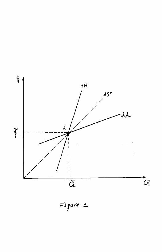
Figure 1 summarizes the initial equilibrium in the noritradables market

in periods 1 and 2.8 Schedule hh depicts the combination of q and Q

consistent with equilibrium in the nontradable goods market in period 1.

Its slope is equal to:

dhh > 0 (10)

qq qq

where EqQ

is an intertemporal cross demand term that captures the reaction

of the demand for N in period 1 (Eq)

to an increase in nontradables

prices in period 2. Given the time separable nature of the utility function

this term is positive.9 rqq

is the slope of the supply curve of N in

period I and Eqq

is the slope of the compensated demand curve in that per-

iod. Consequently the term (r - E ) is also positive. The intuition qq qq

behind the positive slope of hh is the following: an increase in the

price of N in period 2 will affect the consumption discount factor

(6*fI)/m, making consumption in that period relatively more expensive. As a

result, there will be a substitution away from period 2 and towards period 1

expenditure. This will put pressure on the market for N in period 1, and

an incipient excess demand for N in that period will develop. The

reestablishment of nontradable equilibrium in period 1 will require an

increase the relative price ofnontradables.

Schedule HH depicts the locus of qQ compatible with nontradable

market equilibrium in period 2. Its slope is positive and equal to:

7

-Q

/ / / /

V

/ / 1

10

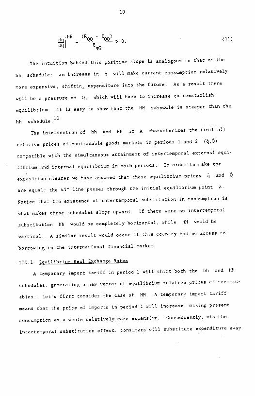
HR (R - E

E >0. (11)

qQ

The intuition behind this positive slope is analogous to that of the

hh schedule: an increase in q will make current consumption relatively

more expensive, shiftir expenditure into the future. As a result there

will be a pressure on Q, which will have to increase to reestablish

equilibrium. It is easy to show that the HR schedule is steeper than the

hh schedule.1°

The intersection of hh and RH at A characterizes the (initial)

relative prices of nontradable goods markets in periods 1 and 2

compatible with the simultaneous attainment of intertemporal external equi-

librium and internal equilibrium in both periods. In order to make the

exposition clearer we have assumed that these equilibrium prices and Q

are equal; the 45 line passes through the initial equilibrium point A.

Notice that the existence of intertemporal substitution in consumption is

what makes these schedules slope upward. If there were no intertemporal

substitution hh would be completely horizontal, while HR would be

vertical. A similar result would occur if this country had no access to

borrowing in the international financial market.

111.1 Etuilibrium Real Exchange Rates

A temporary import tariff in period 1 will shift both the hh and RH

schedules, generating a new vector of equilibrium relative prices of nontrad-

ables. Let's first consider the case of HR. A temporary import tariff

means that the price of imports in period 1 will increase, making present

consumption as a whole relatively more expensive. Consequently, via the

intertemporal substitution effect, consumers will substitute expenditure away

11

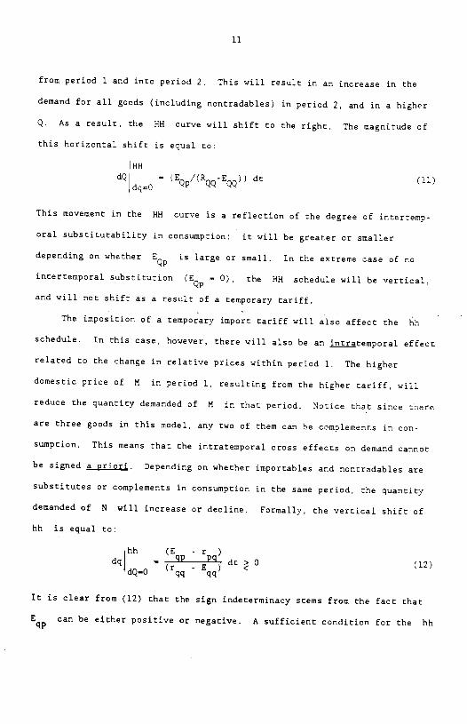
from period I and into period 2. This will result in an increase in the

demand for all goods (including nontrsdsblea) in period 2, and in a higher

Q. As a result, the HR curve will shift to the right. The magnitude of

this horizontal shift is equal to:

RH dQ —

(EQ /(RQQ-EQQ)) dt (11)

dq=O

This movement in the HR curve is a reflection of the degree of intertemp-

oral substitutability in consumption: it will be greater or smaller

depending on whether EQ

is large or small. In the extreme case of no

intertemporsl substitution (EQ

— 0), the RH schedule will be vertical,

and will not shift as a result of a temporary tariff.

The imposition of a temporary import tsriff will also sffect the hh

schedule. In this case, however, there will also be an j.gtemporsl effect

related to the change in relative prices within period 1. The higher

domestic price of M in period 1, resulting from the higher tariff, will

reduce the quantity demanded of M in that period. Notice that since there

are three goods in this model, any two of them can be complements in con-

sumption. This means that the intrstemporal cross effects on demand cannoc

be signed a priori. Depending on whether importables and nontradables are

substitutes or complements in consumption in the same period, the quantity

demanded of N will increase or decline. Formally, the vertical shift of

hh is equsl to:

hh (E -r )

dq — gp - E) dt > 0 (12)

dQ—0 rqq qq

It is clear from (12) that the sign indeterminacy stems from the fsct thst

E can be either positive or negative. A sufficient condition for the hh qp

12

schedule to shift up is that N and M are substitutes, so that Epq

> 0.

On the other hand, a necessary condition for the hh to shift down is that

£ <0. pq

At this level of aggregation, however, the most plausible case corres-

ponds to all goods being substitutes. Notice that even in this case it is

not possible to know whether the hh or the HH schedules will

shift by more (compare (Il) with (12)). In terms of the diagram, if

E > 0, the new equilibrium can be above or below the 4Y line. This pq

gives rise to the possibility of some interesting equilibrium paths for the

RER5. For example, it is possible to observe an "equilibrium overshooting",

where (relative to the no-tariff case) increases by more than . This

would be the case if the hh shifts up by more than what HH shifts to

the right. In such a case the new equilibrium point would be above the 45

line, as illustrated in Figure 2.

Figure 3 illustrates two alternative new equilibria. Point A

characterizes the initial equilibrium. Point B corresponds to the case

when N and M are substitutes and the intrateriiporal effect is strong

enough to shift up the hh schedule significantly. The new (after tariff

imposition) equilibrium schedules are hh and HH. In this case the

temporary import tariff results in a higher relative price of nontradables

in periods 1 and 2. That is, the equilibrium exportables RER appreciates in

both periods, as a result of the temporary tariff. Point C in Figure 3 is

the new equilibrium under the assumption that nontradables and importables

are complements in consumption in period 1 and that this effect dominates so

that the hh schedule will shift down to a position such as RH. Under

this assumption Figure 3 shows that as a result of a temporary tariff the

equilibrium path of the real exchange rate will be characterized by wide

-t

/ / / / / /

/ /

1t,

Nb'

/ /

/

Hk / 452

Fipre

GL

'ti / A

13

swings: it will depreciate in period 1, and it will appreciate

significantly in period 2. Although this path is clearly characterized by

equilibrium movements in each period, observers may think that the RER has

moved in the "wrong direction" in period 1.

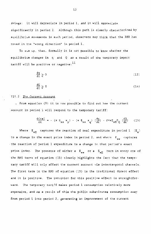
To sum up, then, formally it is not possible to know whether the

equilibrium changes in q and Q as a result of the temporary import

tariff will be positive or negative:11

(13)

(14)

111.2 The Current Account

From equation (9) it is now possible to find out how the current

account in period 1 will respond to the temporary tariff:

- .m E m - (irE ir - 5*irE ii (15) dt irir p inc q dt irflQ dt

Where E11 captures the reaction of real expenditure in period 1 (E)

to a change in the exact price index in period 2, and where E captures

the reaction of period 1 expenditure to a change in that period's exact

price index. The presence of either a E or a E term in every one of inc rr

the RHS terms of equation (15) clearly highlights the fact that the tempo-

rary tariff will only affect the current account via intertemporal channels.

The first term in the RHS of equation (15) is the traditional direct effect

and it is positive. The intuition for this positive effect is straightfor-

ward. The temporary tariff makes period I consumption relatively more

expensive, and as a result of this the public substitutes consumption away

from period 1 into period 2, generating an improvement of the current

14

account balance in period I. The magnitude of this effect will depend both

on the term E and on the initial share of imports on period 1 mm

expenditure m.

The second and third terms on the RHS of equation (15) are indirect

effects, that operate via changes in periods I and 2 equilibrium real

exchange rates. Since, as was established above, the signs of (dq/dc) and

(dQ/dt) cannot be determined a priori., the signs of these two terms in (15)

are generally undetermined, as will be the sign of the current account

equation (15) as a whole. However, the interpretation of these two indirect

terms is quite straightforward. If the temporary tariff results in an

equilibrium real appreciation in period 1, (dq/dt) > 0, there will be an

additional force towards a current account improvement. The reasoning is

again simple. If the temporary tariff results in a higher equilibrium price

of nontradables in period 1 (i.e., in a real appreciation in 1), there will

be substitution away from period 1 expenditure, generating an improvement in

the current account in that period. The third term on the RHS relates the

change in period 2's RER to period l's current account. If as a consequence

of the temporary tariff Q increases, there will be a tendency to substi-

tute expenditure away from period 2 into period 1, generating forces that

will tend to worsen the current account in period 1. Notice that the

presence of these two terms involving the real exchange rate introduce

important differences to the more traditional intertemporal analysis, as the

one pioneered by Svensson and Razin (1983).

The total effect of the temporary import tariff on period l's current

account will depend on the strength of the intertemporal price effects, on

the initial expenditure on imports and nontradables, and on the effects of

the tariff on the RER vector. It is possible, however, that as a

15

consequence of the temporary import tariff the current account will worsen

in the period when the tariffs are imposed, generating a quasi-perverse

effect. This result suggests that policy makers should be very careful when

imposing temporary trade restrictions as a way to improve the current

account.

IV. External Terms of Trade, Real Exchange Rates and the Current Account

The discussion in Section III has concentrated exclusively on

substitution channels, ignoring income effects. This was possible thanks to

the simplifying assumption of a zero initial tariff. However, in real world

situations income effects are important and can have an important influence

on the current account. There,are two circumstances when income effects

will be particularly important: when there are tariff changes in the pre-

sence of large initial tariffs, and when there are discurbancesto external

terms of trade -- the world price of importables relative to exportables.

In this section we analyze the way in which the temporary disturbances to

the external terms of trade affect the current account. The analyais

focuaes on the role of income effecta and the results obtained are compared

to those of Section III. As in the previous section, the discussion

proceeds by steps: we first inquire how a temporary shock to the external

terms of trade affects the vector of equilibrium real exchange rates. 1e

then discuss how period 1 current account is affected by this shock.

IV.l Equilibrium Real Exchange Rstes

When there are income effects the diagrammstic apparatus of Section III

cannot be usedto analyze the behavior of equilibrium RERs. Still sssurning

that t — T — 0, a temporsry shock in the external terms of trade will

affect the vector of equilibrium RERs in the following way:12

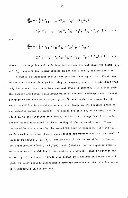
16

-r 'R -E )+E E dp* A pg pq QQ QQ QpQq

+ () (E - r) (EqQ rrQ E11 +

1tqElti(RQQ -

EQQ)) 0 (16)

and

-r )E +E (r -E )) dp* A pq pq qQ Qp qq qq

+ (E - r) [q EQq E, + (rqq

-

Eqq) tIQEII& 0 (17)

where A is negative and is defined in footnote 11, and where the terms E

and E0 capture the income effects in periods 1 and 2, and are positive.

A number of important results emerge from these equations. First, due

to the existence of foreign borrowing, a temporary terms of trade shock that

only increases the current international price of imports, will affect both

the current and future equilibrium value of the real exchange rate. Second,

contrary to the case of a temporary tariff, even under the assumption of

substitutability in demand everywhere, the change in the relative price of

nontradables cannot be signed. The reason for this is, of course, that in

addition to the substitution effects, we now have a (negative) first order

income effect associated to the worsening of the terms of trade. These

income effects are given by the second RI1S term in equations (16) and (17)

As is usually the case these income effects are proportional to the level of

imports in period 1 (E-r), Notice that if the income effect dominates

the substitution effect, (dq/dp*) and (dQ/dp*) can be negative even if

we assume substitutability in consumption everywhere. This is because the

worsening of the terms of trade will result in a decline in demand for all

goods in every period, generating a downward pressure on the relative price

of nontradables in all periods.

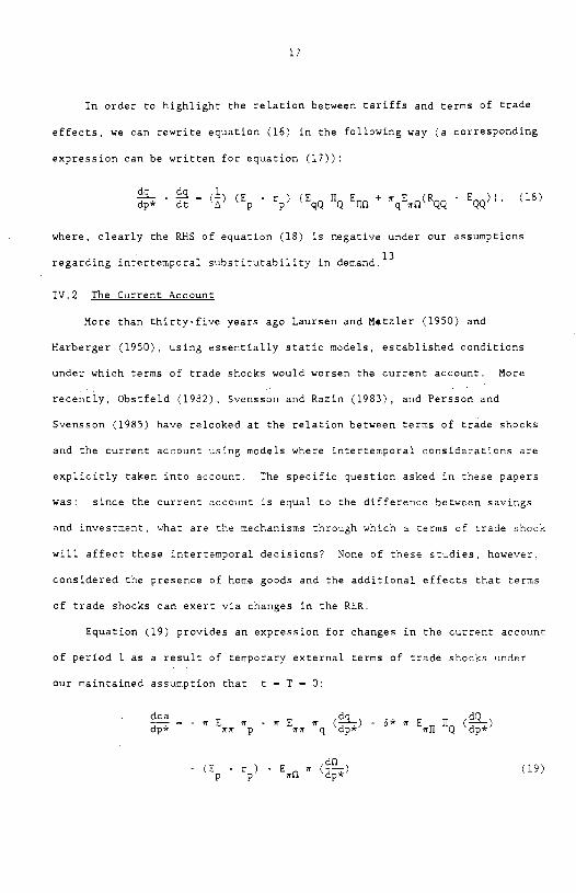
17

In order to highlight the relation between tariffs and terms of trade

effects, we can rewrite equation (16) in the following way (a corresponding

expression can be written for equation (1?)):

- — () (5 - r) (EqQ fl E + tqEQ(RQQ - E)), (18)

where, clearly the Ri-IS of equation (18) is negative under our assumptions

regsrding intertemporal substitutability in demand.13

IV.2 The Current Account

More than thirty-five years ago Lsursen and Metzler (1950) snd

Harberger (1950), using essentially static models, established conditions

under which terms of trade shocks would worsen the current account. More

recently, Obstfeld (1982), Svensson and Razin (1983), snd Persson and

Svensson (1985) have relooked at the relation between terms of trade shocks

and the current account using models where incercemporsl considerations are

explicitly taken into account. The specific question asked in these papers

was: since the current account is equsl to the diffetence between savings

and investment, what are the mechanisms through which a terms of trade shock

will affect these intercemporsl decisions? None of these studies, however,

considered the presence of home goods and the additional effects that terms

of trade shocks can exert via changes in the RER.

Equation (19) provides an expression for changes in the current account

of period 1 as a result of temporary external terms of trade shocks under

our maintained assumption that t — T — 0:

42! - E - E (42-) - 5* E r (42_) dp* its p irs q dp* itO Q dp*

dO - (E - r ) - E it

p p itO dpw

18

It is clear from equation (19) , that in the present model it is not

possible to know with certainty whether a temporary worsening in the terms

of trade will improve or worsen the current account. The first three R}{S

terms of equation (19) are equivalent to those in equation (15) for the

temporary tariff case, and their economic interpretation is virtually the

same. The fourth RHS term in (19) is equal to period 1 imports and s.ce it

is preceded by a minus sign, it is negative. The last R1-{S term in (19) cap-

tures the (negative) income effect generated by a deterioration of the terms

of trade, and is positive since (di2/dp*) < 0 (i.e., the negative terms of

trade shock reduces aggregate utility and real income) . These last two terms

capture the effects of the reduction in expenditure in both periods on the

current account in period 1: the decline in wealth prompted by the terms of

trade shock will generate forces towards improving the current account in

that period.

It is interesting to compare the effects of a temporary external terms

of trade shock to those obtained from a permanent disturbance to the world

relative price of imports. In the case in which dp* — dP* the change in

the current account of period 1 will be:

dca dca — (_.-) - (5*m E0 fIr) permanent temporary

Notice that, as before, the response of the current account in period I

to a mermanent terms of trade shock cannot be signed unequivocally. In this

model, even if there is a permanent terms of trade shock we cannot know

priori whether the first period current account will improve or worsen.

What we do know from (20), however, is that, whatever the sign is, the

magnitude of the change will be different than in the case of a temporary

shock. Naturally, this is due to the fact that the term (6*irEfl) is

19

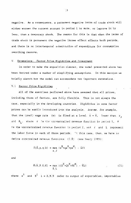
negative. As a consequence, a permanent negative terms of trade shock will

either worsen the current account in period 1 by more, or improve it by

less, than s temporary shock. The reason for this is that when the terms of

trade shock is permanent the negative income effect affects both periods,

and there is no intertemporsl substitution of expenditure for consumption

smoothing reasons.

V. Extensions: Factor Price Rigidities and Investment

In order to make the exposition clearer, the model presented above has

been derived under a number of simplifying assumptions. In this section we

briefly sketch how the model can accommodate two important extensions.

V.1 Factor Price Rigidities

All of the exercises performed above have assumed that all prices,

including those of factors, are fully flexible. This is not always the

case, especially in the developing countries. Rigidities in some factor

prices can be easily introduced into the analysis. Assume, for example,

that the (real) wage rate (w) is fixed at a level — , lower than

and RL where r is the unconstrained revenue function in period 1, R

is the unconstrained revenue function in period 2, and 9 and L represent

the labor force in each of those periods. n this case, then, we have to define constrained revenue functions (8,R) (see Neary 1985):

— max {5Xq5Np5M) - w2) si and

a(w,P,Q;K) — max ((5XQ5N÷85M) - WL) S,L

where 5 and Si i — X,M,N refer to output of exportables, importables

20

and nontradables in periods 1 and 2. Now the nontradable market equilibrium

conditions need to be replaced by:

r —E. (22) q q

Neary (1905) has shown that under fixed factor prices the following relation

exists between restricted and unrestricted revenue functions:

— r[p,q,.2(w,p,q,k)] - w2(w,p,q,k) (23)

where .2 is the amount of labor employed in the constrained case. Once the

revenue functions have been redefined in this way it is easy to find how the

relative price of nontradables reacts to a tariff change in an economy with

fixed real wages. After this effect has been found the way the current

account will react can be derived in the same way as in Sect-ion IV above.

For a number of years trade theorists have been preoccupied with the

relation between tariffs and employment (van Wijnbergen 1987). In the model

developed in this paper, if wages are flexible, tariffs have no effects on

aggregate employment. However, if there is real wage rigidity tariffs will

indeed have an effect on the level of total employment in the economy. For

example, equation (24) gives the response of labor employed in period I to a

temporary tariff in that period:

— - (2/r) - (jq/) (dq/dt) (24)

where the term (dq/dt) captures the change in the relative price of N in

period 1 to that period's tariff increase. Both and rjq

are

Rybczinski type terms whose signs will depend on factor intensities.

Depending on the sign of (dq/dc) and on factor intensities in the

different sectors (d2/dr) can be positive or negative.

21

V.2 Investment

Since the discussion presented above has ignored investment, the

current account in each period is equal to savings in that particular

period. Investment, however, can be introduced in a straightforward

fashion. Once investment is added to the analysis, the intertemporal budget

constraint has to be altered and an equation describing the process govern-

ing investment decisions has to be added to our system. Denoting investment

by I and aaauming that there is time to build, the intertemporal budget

constraint becomes (where v is now the vector of factors of production

other than capital):

r(l,p,q;k,v) + 5*R(l,P,Q;k+I,v) + t(E-r) +

- 1(5*) — E(x(l,p,q),S*fl(l,P,Q),O] (25)

Possibly the simplest way to deal with investment is by assuming that

investment decisions are governed by the condition that in equilibrium

Tobin's "q" equals 1. Further assuming that investment goods correspond to

the numeraire good, the investment equation can be written in the following

way:

1 (26)

The manipulation of (25) and (26) and the two conditions for equilibrium in

the nontraded goods market in period 1 and 2 will now yield the correspond-

ing expressions for changes in the RERs and the current account. In this

case the current account equation should be modified by subtracting I to

the RHS of equation (9).

22

VI. Concluding Remarks

In this paper I have developed an intertemporal, fully optimizing model

of a small open economy with nontradable goods to analyze how temporary

terms of trade shocks affect the current account. The analysis distinguish-

ed between disturbances to the internal terms of trade, generated by tariff

changes, and disturbances to the external terms of trade. In this general

setting changes in the (equilibrium) real exchange rate - - or relative price

of nontradables - - provided an important channel through which a change in

the terms of trade will influence the current account, For this reason the

analysis of the current account behavior was preceded by an analysis of the

determinants of real exchange rates. It was shown that in this intertempor-

al setting a temporary tariff will affect the equilibrium real exchange rate

both in the current and future periods. However, it is not possible to know

a priori the direction of this effect. In fact, it is possible that,

contrary to popular belief, a temporary tariff will result in a real

exchange rate depreciation in the current period, which is later reversed.

The analysis has shown that it is possible for a temporary import

tariff to worsen the current account in the period when it is imposed. This

indicates that policy makers should be particularly careful when using

temporary protectionist policies for balance of pavntents purposes. Not only

wIll these policies result in welfare reducing inefficiencies, but may very

well fail to achieve their intended objective of improving the current

account and the degree of competitiveness.

The model can be expanded in several way The cases of anticipated

and permanent terms of trade shocks follow directly from the analysis

presented here. Two interesting extensions are related to increasing the

dimensioriality of the model either in terms of periods and/or countries.

23

The case of more than two periods is analytically straightforward; the

algebra, however, is messier. In that case the scope for unconventional

results is expanded, since with mote than two periods it is possible to have

intertemporal complementarity in demand. The case of two (large) countries

is slightly more difficult, since world market clearing conditions have to

be incorporated. An interesting feature of the large country case is that

even if tariffs are initially zero, tariff changes will still result in

first order income effects. The reason, of course, is that in the large

country case tariff changes will affect the international terms of trade.

24

FOOTNOTES

10n the recent discussions on protectionism in the U.S. see, for

example, the aI1 Street Journal, Monday, May 16, 1988, page 1.

2See Edwards (1988a) for a detailed analysis of the effects of tariffs

and exchange controls on the balance of payments in a group of Latin

American countries.

3Svensson and Razin (1983) van Wijnbergen (1984) and Edwards and van

Wijnbergen (1986), among others, have emphasized the intertemporal nature of

the current account, These papers, however, have only dealt with two goods

economies. On intertemporal models of the current account with nontradables

see Frenkel and Razin (1986, 1987), Edwards (1987) and Ostry (1988).

4See, however, Edwards (forthcoming) for a related model where the

government uses tariffs proceeds to finance its own consumption.

5See Dixit and Norman (1980) for the use of duality in static trade

models. Svensson and Razin (1983) and Edwards and van Wijnbergen (1986) use

duality in intertemporal models without nontradables.

we allow some of the goods to enter as an input in the production

of another good, some of these cross derivatives could be negative.

However, in order to maintain the analysis at a simple level, in what

follows we ignore that possibility.

7Notice that implicit in this definition is the requirement of full

employment.

8Thjs type of diagram has a long tradition in international economics.

See, for example, Dornbusch (1980), Llaaparanta and Kahkonen (1986), and van

Wijnbergen (1987).

25

9The exact expreaaion for EQ ia obtained after taking the derivative

of the equation E — E it

q itq

10See, for inatance, Edwards (1987), Edwards (forthcoming) and Ostroy

(1988).

11 Formally,

— - () ((Epq -

rpq)(R - E) + EQpEqQ)

— - (i) CE (E - r ) + E (r - E )) dt A Qq pq pq Qp qq qq

where A — ((rqq -

Eqq)(RQQ - E) -

EQqEqQ} < O

12Naturally, when there is an external terms of trade shock, even if

initial tariffs are equal to zero there will be s non-zero income effect.

13Edwards (1987) develops anslogous expressions for the effect of

anticipated and permanent external terms of trade shocks on the vector of

equilibrium RERs.

26

References

Dixit, A., and V. Norman (1980), Theory of International Trade, Cambridge

University Press.

Dornbusch, R. (1980), Open Economy Macroeconomics, New York: Basic Books.

Edwards, S. (1987), "Anticipated Protectionist Policies, Real Exchange Rates

and the Current Account," NBER Working Paper No. 2214.

_________ (1988a), "Exchange Controls, Devaluations and Real Exchange

Rates: The Latin American Experience," Economic Development and Cultural

Change (forthcoming)

__________ (1988b), "Economic Liberalization and the Real Exchange Rate in

Developing Countries," in R. Findlay (ed.), Debt. Stabilization and

justment; Essays in Memory of Carlos Diaz-A1eandrp, Oxford: Black'well

(forthcoming)

_________ (1988c), "Tariffs, Capital Controls and Equilibrium Real Exchange

Rates," revised version of NBER Working Paper No, 2162 (UCLA Dept. of

Economics)

(forthcoming), Real Exchange Rates. Devaluation and Adlustment.

Edwards, S., and S. van Wijnbergen (1986), "The Welfare Effects of Trade and

Capital Market Liberalization," International Economic Review vol. 27,

No. 1, February: 147-148.

_________ (1987), "Tariffs, The Real Exchange Rate and the Terms of Trade:

On Two Popular Propositions in International Economics," Oxford Economic

Papers, vol. 39, No. 3, September: 458-464.

Frenkel, J. and A. Razin (1986), "Fiscal Policies and Real Exchange Rates in

the World Economy,' NEER Working Paper No. 2065 (December).

_________ and _________ (1987), FIscal Policy and the World Economy,

Cambridge, MA: MIT Press.

Haaparanta, P., and J. Kahkonen (1986), "Liberalization of Capital Movements

and Trade: Real Appreciation, Employment and Welfare," Wider Working

Paper.

Narberger, AC. (1950), "Currency Depreciation, Income, and the Balance of

Trade," Journal of Political Economy, vol. 58, No. 1, February: 47-60.

Laursen, S., and L. Metzler (1950), "Flexible Exchange Rates and the Theory

of Employment," Review of Economics and Statistics, vol. 32, No. 4,

November: 281-299.

27

Neary, P. (1985), "International Factor Mobility, Minimum Wage Races and

Factor-Price Equalization: A Synthesis," quarterly Journal of Economics,

vol. 100, No. 3, August: 551-570.

Obstfeld, N. (1982), "Aggregste Spending and the Terms of Trade: Is There a

Laursen Metzler Effect?" Quarterly Journal of Economics, vol. 97, No. 2,

May: 251-270.

Ostry, J. (1988), "Terms of Trade and the Current Account in an Optimizing

Model," Working Paper, IMF.

Persson, T. , and LEO. Svensaon (1985), "Current Account Dynamics and the Terms of Trade: Harberger-Laursen-Metzler Two Generations Later,"

Journal of Political Economy, vol. 93; February: 43-65.

Razin, A., and LEO. Svenson (1983), "Trade Taxes and the Current Account," Economics Letters, vol. 13, No. 1: 55-57.

Svensson, LEO., and A. Razin (1983), "The Terms of Trade and the Current Account: The Harberger-Laursen-Metzler Effect," Journal of Political

Economy, vol. 91, No. 1, February: 97-125.

van Wijnbergen, S. (1984), "The Dutch Disease: A Disease After All?"

Economic Journal, vol. 94, No. 373, March: 41-55.

_________ (l985a), "Taxation of International Capital Flows, the

Intertemporal Terms of Trade and the Real Price of Oil," Oxford Economic

Papers, vol. 37, No. 3, November: 382-390.

_________ (l985b), "Capital Controls and the Real Exchange Rate," CPD WP

el985-52, World Bank.

<1987), "Tariffs, Employment and the Current Account: Real Wage Resistance and the Macroeconomics of Protectionism,

" International Economic Review, vol. 28, No. 3, October: 691-706.