seasonal forecasts of sea ice - candac · 2017-07-19 · cansips skill of sea ice area forecasts...
TRANSCRIPT

https://weather.gc.ca/saisons/image_e.html?img=s123pfe1t_cal_comb

Outline:
• Why care about forecasting sea ice 1-12 months ahead?
• Potential sources of sea ice predictability
• Tools used to predict sea ice
• Forecast skill quantification
• Some recent progress (CanSISE)

Increased marine accessibilitySept. 2012Sept. 1980
Top: nsidc.orgBottom: Sigmond et al. 2016, Geophys. Res. Lett.
Observed trends (1979-2010)
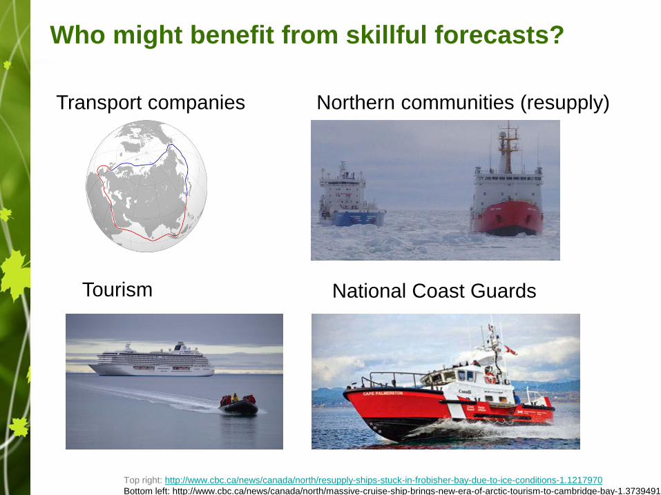
Who might benefit from skillful forecasts?
National Coast Guards
Transport companies Northern communities (resupply)
Tourism
Top right: http://www.cbc.ca/news/canada/north/resupply-ships-stuck-in-frobisher-bay-due-to-ice-conditions-1.1217970Bottom left: http://www.cbc.ca/news/canada/north/massive-cruise-ship-brings-new-era-of-arctic-tourism-to-cambridge-bay-1.3739491
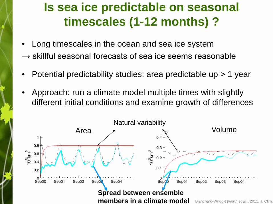
Is sea ice predictable on seasonal timescales (1-12 months) ?
• Long timescales in the ocean and sea ice system → skillful seasonal forecasts of sea ice seems reasonable
• Potential predictability studies: area predictable up > 1 year
• Approach: run a climate model multiple times with slightly different initial conditions and examine growth of differences
Spread between ensemble members in a climate model
Area Area Volume Natural variability
Blanchard-Wrigglesworth et al. , 2011, J. Clim.

Potential sources of predictability:
1) Long term trend due to external forcings
2) Persistence of sea ice anomalies (~months)
3) Advection (mean circulation)
Guemas et al, 2016, Q.J.R. Meteorol. Soc.
1) Beaufort gyre2) Transpolar Drift Stream3) Laptev Sea Gyre4) East Siberian circulation
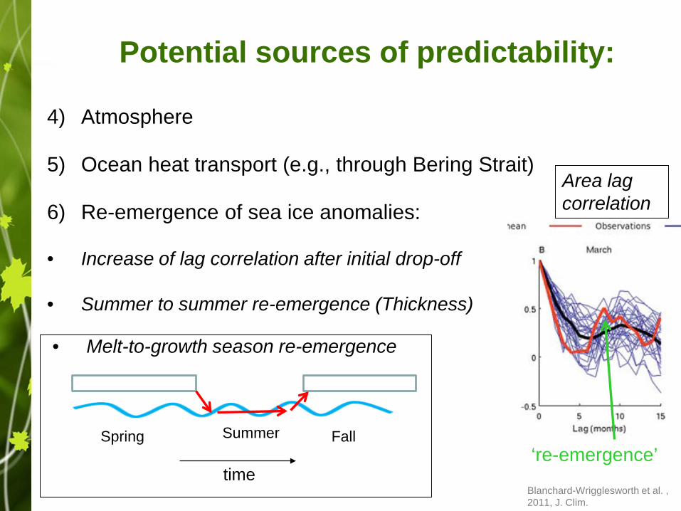
Potential sources of predictability:
4) Atmosphere
5) Ocean heat transport (e.g., through Bering Strait)
6) Re-emergence of sea ice anomalies:
• Increase of lag correlation after initial drop-off
• Summer to summer re-emergence (Thickness)
Blanchard-Wrigglesworth et al. , 2011, J. Clim.
Summer FallSpring
time
• Melt-to-growth season re-emergence
‘re-emergence’
Area lag correlation

Tools/methods used to produce forecasts:1) Analog year method
2) Statistical models (Multi Linear Regression models)• Built upon statistical relationships derived from historical observations• May not be valid today (future) because of rapidly changing Arctic
• look for year with similar conditions like freeze-up date, ice thickness, summer air temperature outlook
• Ran out of analog years by 2007

Dynamical models:
• Global climate models (numerical models that represent interactions between atmosphere, ocean, sea ice)
• Initialized with observed climate state
• Aspects of weather forecasting (initial value problem) and long-term climate projections (boundary value problem, interactive ocean)
• Dynamical models used for seasonal forecasting (temperature, precipitation) since ~1990s, but not suitable for sea ice forecasts (not interactive)

Canadian Season to Inter-annual prediction System (CanSIPS)
• ECCC’s operational seasonal forecasting system since Dec 2011
• One of the first to include interactive sea ice
• Based on 2 global climate models (CanCM3/4, cancellation of errors improved skill)
• Seasonal forecasting is a probablistic problem run multiple realizations (10 for each model) with slightly different initial conditions

Hindcast dataset - a key ingredient
• Purposes of Hindcasts (re-forecasts of past):1) Skill quantification2) Statistical bias correction (mean, distribution)
• CanSIPS: hindcasts initialized at start of each month since 1979 (forecast range: 12 months)
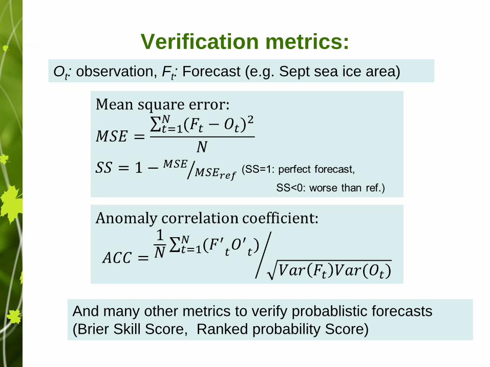
Verification metrics:Ot: observation, Ft: Forecast (e.g. Sept sea ice area)
And many other metrics to verify probablistic forecasts (Brier Skill Score, Ranked probability Score)
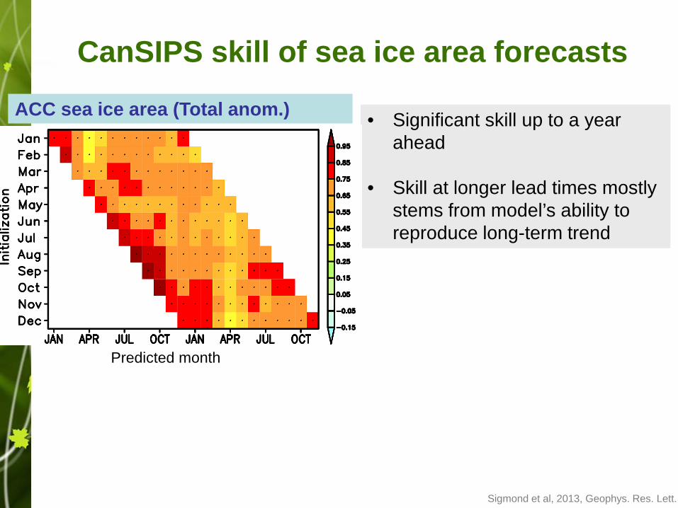
CanSIPS skill of sea ice area forecasts
• Significant skill up to a year ahead
• Skill at longer lead times mostly stems from model’s ability to reproduce long-term trend
ACC sea ice area (Total anom.)
Predicted month
Sigmond et al, 2013, Geophys. Res. Lett.

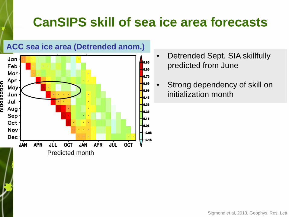
CanSIPS skill of sea ice area forecasts
• Detrended Sept. SIA skillfully predicted from June
• Strong dependency of skill on initialization month
• Substantial skill at long lead times for winter predictions
• Model beats persistence
ACC sea ice area (Detrended anom.)
Predicted month
Sigmond et al, 2013, Geophys. Res. Lett.

CanSIPS skill of sea ice area forecasts
• Detrended Sept. SIA skillfully predicted from June
• Strong dependency of skill on initialization month
• Substantial skill at long lead times for winter predictions
• Model beats persistence
ACC sea ice area (Detrended anom.)
Predicted month
• These features appeared to be robust for other systems (CFSv2: Wang et al. 2013, MetOffice: Peterson et al. 2014, GFDL: Msadek et al 2014)
• But not clear if dynamical model provide skillful seasonal forecasts of user-relevant sea ice quantities

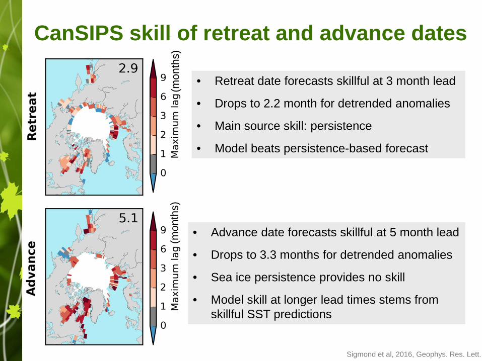
CanSIPS skill of retreat and advance dates
• Retreat date: First calendar day with SIC < 50%
• Advance date: First calendar day with SIC > 50%
• Maximum lead time with skill:
[climatological date] – [earliest initialization month with skill]
ACC>0.3 (p=0.05)
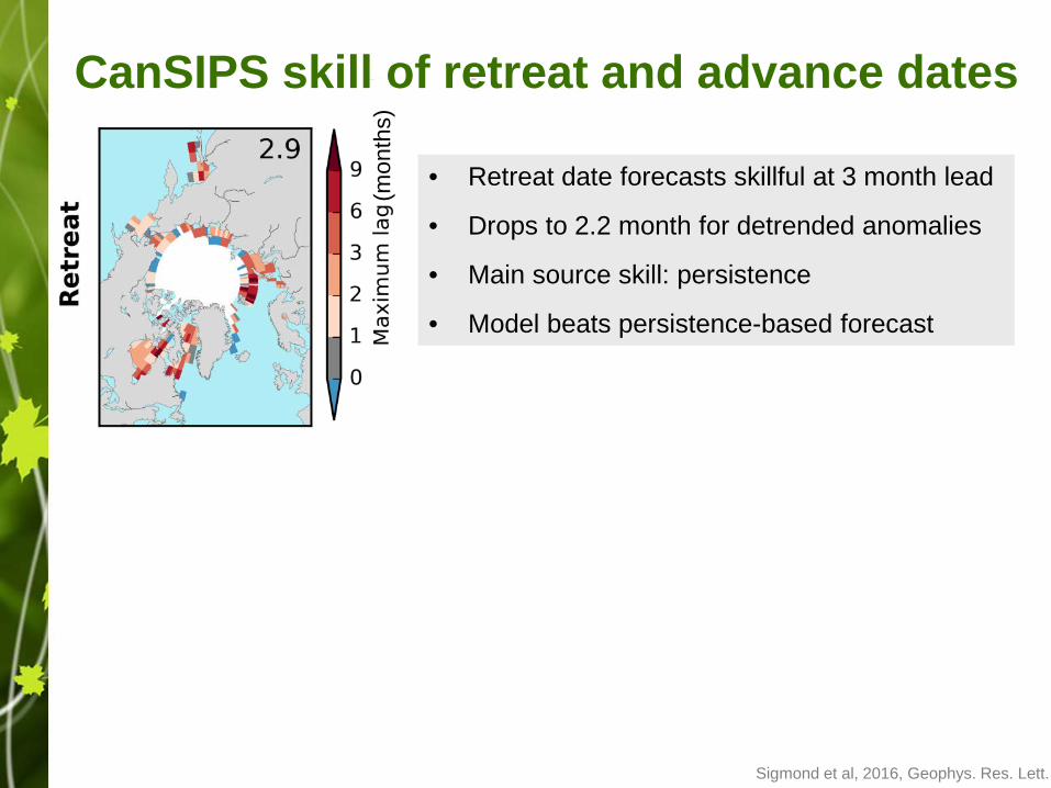
• Retreat date forecasts skillful at 3 month lead
• Drops to 2.2 month for detrended anomalies
• Main source skill: persistence
• Model beats persistence-based forecast
• Advance date forecasts skillful at 5 month lead
• Drops to 3.3 months for detrended anomalies
• Sea ice persistence provides no skill
• Model skill stems from skillful SST predictions
CanSIPS skill of retreat and advance dates
(mon
ths)
(mon
ths)
Sigmond et al, 2016, Geophys. Res. Lett.
• Retreat date forecasts skillful at 3 month lead
• Drops to 2.2 month for detrended anomalies
• Main source skill: persistence
• Model beats persistence-based forecast
• Advance date forecasts skillful at 5 month lead
• Drops to 3.3 months for detrended anomalies
• Sea ice persistence provides no skill
• Model skill at longer lead times stems from skillful SST predictions
CanSIPS skill of retreat and advance dates
(mon
ths)
(mon
ths)
Sigmond et al, 2016, Geophys. Res. Lett.

Recent developments under CanSISE (Dirkson, Merryfield)
• Development of methods to post-process CanSIPS output to obtain calibrated sea ice probability forecasts
• Resolving issue with operational forecasts (inconsistency between hindcasts and operational forecasts)
SIT climatology (original)Reconstructed PIOMAS
• Improved sea ice thickness initialization (time-varying instead of climatology)
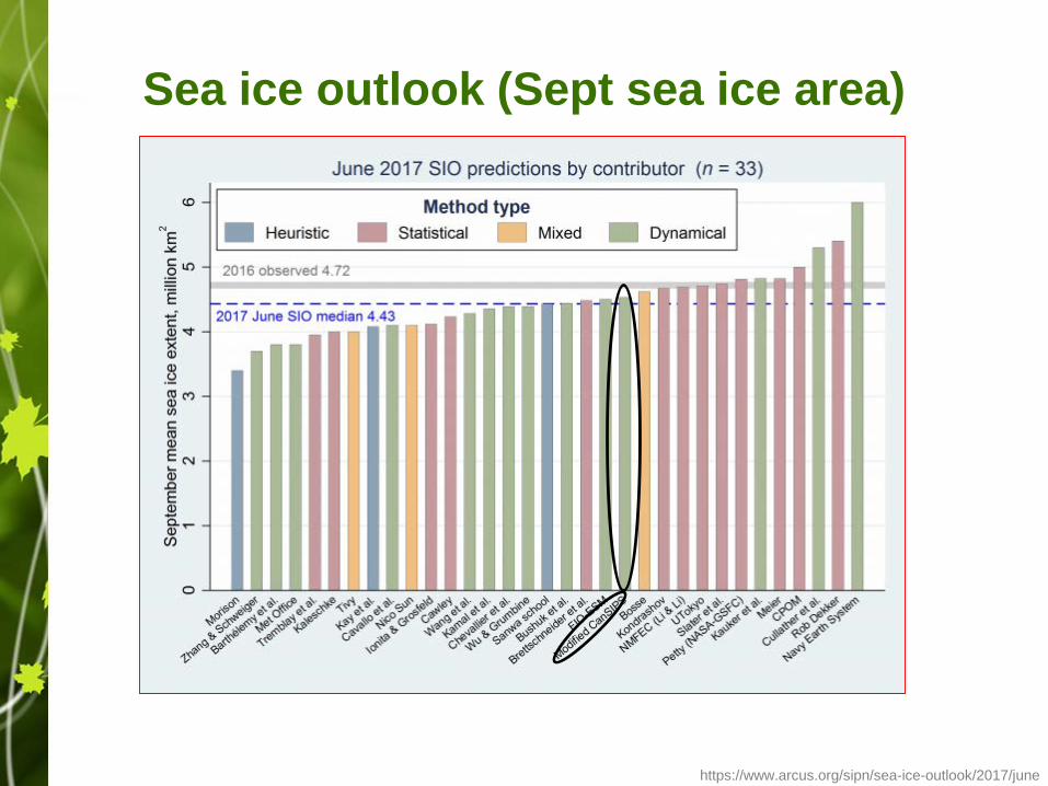
Sea ice outlook (Sept sea ice area)
https://www.arcus.org/sipn/sea-ice-outlook/2017/june

Sea ice outlook (Sept sea ice probability)
https://www.arcus.org/sipn/sea-ice-outlook/2017/june
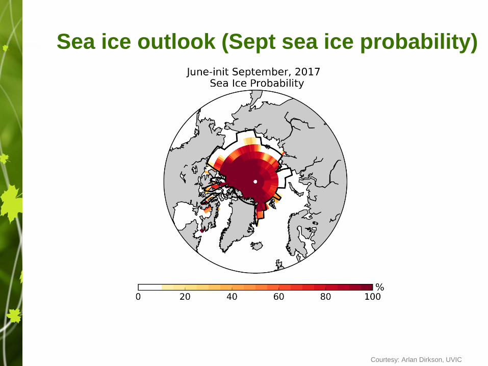
Sea ice outlook (Sept sea ice probability)
Courtesy: Arlan Dirkson, UVIC

Future developments
• Improve models (new ocean/ice model, higher resolution, better parameterization of relevant processes such as melt ponds)
• Improve observations (verification, initialization)
• Improve bias correction and calibration procedures
• Interact with end-users to come up with more user-relevant sea ice products (balance between desires and feasibility)