Seasonal Asset Allocation:

Evidence from Mutual Fund Flows

Abstract

Investment managers and finance researchers alike are interested in the flow of invest-ments into and out of mutual funds. Fund managers have a financial incentive to attractcapital under their management, while academic researchers are interested in mutual fundflows partly due to their fascination with the relationship between fund flows and fundperformance. In light of the interest, we closely examine the determinants of fund flows,revealing a substantial regularity in mutual fund investment patterns that has previouslygone unnoticed: seasonally varying flows between funds of different risk characteristics. Theseasonality in flows is shown to be consistent with the influence of seasonal affective disorder,SAD, on investor sentiment. According to extensive clinical research on SAD, many millionsof people suffer from depression or “winter blues” when the hours of daylight shrink in thefall, and recover as the days lengthen in the winter. Furthermore, experimental evidenceshows that depression is in turn associated with increased risk aversion. This SAD / riskaversion linkage implies movements of funds from riskier to safer investments as risk aversionrises in the fall, and from safer to riskier investments as risk aversion subsides in the winter.This paper examines seasonality in the movement of investment dollars into and out of bothrisky equity mutual funds and safe bond mutual funds to see if they correspond to the impli-cations of SAD. We find economically and statistically significant seasonal patterns in mutualfund flows consistent with the SAD hypothesis, and we find that modeling the SAD-relatedseasonal adds considerably to our ability to explain flows. Overall, this provides powerfulnon-return-based evidence of the importance of SAD for seasonality in financial markets ingeneral, and potentially for helping to explain fund return persistence in particular. Further,the results have implications for the timing of advertisements by the mutual fund industrywhich spends over half a billion dollars each year encouraging investors to purchase mutualfunds.

The mutual fund industry spends more than half a billion dollars a year advertising to

attract investment inflows. (See Pozen, 2002.) The benefits to attracting capital are clear: a

conservative estimate of the management fees collected by mutual funds in the United States

in 2003 is 50 billion dollars on close to 7.5 trillion dollars under management.1 Jain and Wu

(2000) demonstrate that advertised funds attract significantly more new investments than

the average fund. Gallaher, Kaniel, and Starks (2004) show that advertising is significantly

related to fund family flows. Given the formidable magnitudes of advertising budgets and

the even grander scale of the management fees they seek to attract, it is conceivable that if

fund managers had access to more information about determinants of flows of mutual fund

investment, they would be keen to use it to tailor their promotion efforts.

Among academics, interest in mutual fund flows extends beyond the influence of adver-

tising. For instance, in a growing literature, researchers have documented a relationship

between mutual fund flows and subsequent mutual fund performance. Gruber (1996) and

Zheng (1999) find that funds with recent inflows subsequently perform better than those

with recent outflows. Wermers (2003) demonstrates this phenomenon, known as the smart

money effect, may arise because money that flows into the hands of managers of a fund

that has performed well is often used to purchase more well-performing stocks (which are

themselves persistent), leading to further good performance for the fund. Given the evidence

that performance may depend on prior flows, it is essential to understand the determinants

of fund flows to fully understand the predictability of fund performance.

In light of the commercial and academic interest in the flow of capital into and out of

mutual funds, in this study we dig deeply into the determinants of mutual fund flows them-

selves. Prior research has found fund flows are partly explained by past or contemporaneous

returns (either returns to the fund or returns to the market as a whole). See, for instance,

Ippolito (1992) and Sirri and Tufano (1998). Some studies, including Del Guercio and Tkac

1According to the Investment Company Institute (2003), the average expense ratio charged across 46large equity mutual funds is 0.7 percent, while according to the Securities and Exchange Commission (2000),the average may be closer to 1 percent across all funds.

1

(2001) and Bergstresser and Poterba (2002), have found various fund-specific characteristics

help explain fund flows. Further, many researchers have noticed that a prominent feature of

all classes of fund flows is persistence, as documented by Warther (1995), Karceski (2002),

and others.

We examine the possibility of a regularity in mutual fund flows that has gone hitherto

unnoticed. The motivation for the regularity is based on work by Kamstra, Kramer, and Levi

(2003, 2004) demonstrating novel seasonal patterns in returns to publicly traded stocks and

bonds that are economically and statistically significant, and very robust. As we discuss in

detail below, if KKL’s rationale for the seasonal patterns in stock and bond returns is valid,

we should observe seasonal patterns in the flow of funds between stock and bond mutual

funds that correspond to those documented in this paper.

KKL suggest the pattern they find in stock and bond returns arises as a consequence

of seasonal depression among investors. Medical evidence firmly demonstrates that as the

number of hours of daylight drops in the fall, about ten percent of the population becomes

depressed with a condition known as seasonal affective disorder, or SAD.2 It has further

been shown that depression leads to risk averse behavior, both in general and in the con-

text of making financial decisions in particular.3 Given the links between seasonal cycles in

daylight, depression, and risk aversion, it is conceivable that with the reduction of daylight

in the fall, SAD-affected investors sell risky stocks and buy safer assets like bonds. When

daylight becomes more abundant in the new year and SAD-influenced investors begin revert-

ing to normal levels of risk aversion, those investors would then sell bonds and resume risky

holdings. KKL (2003) and Garrett, Kamstra, and Kramer (2004) find evidence consistent

with this hypothesis in international stock market returns, and KKL (2004) find support in

US Treasury bond returns, even after controlling for established market seasonalities such

as tax- loss selling. On average, stock market returns are lowest and bond returns are high-

2The nature, incidence, and cause of SAD are discussed in a wide range of articles in the medical andpsychology literatures well surveyed by Lee et. al. (1998).

3Examples include Harlow and Brown (1990) and Wong and Carducci (1991).

2

est during the fall months when the number of hours of daylight is falling toward its annual

minimum. Mean stock returns are then highest and bond returns lowest as daylight becomes

more plentiful through winter. That is, stock and bond returns display reverse seasonal pat-

terns, something that is difficult to explain without seasonal variations in risk aversion. We

expect fund flows to exhibit similar seasonality, with opposing flows of investment into and

out of mutual funds at opposite extremes of the risk spectrum as investors act on seasonal

changes in their risk aversion.

In this paper we consider whether there is evidence from mutual fund flows to support

the SAD hypothesis. By studying flow of funds instead of asset returns, we examine a set of

data unrelated to KKL’s prior findings. In particular, we consider whether there are seasonal

regularities in the flow of investments into and out of safe and risky mutual funds that are

consistent with the SAD-based argument and with previously documented seasonal patterns

in stock and bond returns. We hypothesize that capital is flowing out of risky equity mutual

funds and into safe bond mutual funds when reduced daylight leads to higher levels of risk

aversion for some investors, and that capital is flowing out of bond funds and back into

stock funds when daylight becomes more abundant. We find evidence supporting such flows,

reinforcing the importance of seasonal depression and hence time-varying risk aversion in

determining individuals’ portfolio choices and for financial markets in general.

The remainder of the paper is organized as follows. In Section 1, we describe seasonal

affective disorder and explain how it can translate into an economically significant influence

on a SAD-affected investor’s choice of assets. In Section 2, we briefly define the measures we

use to capture the impact of SAD on investment decisions. In Section 3 we present evidence

that the flow of capital into and out of mutual funds follows a seasonal pattern consistent

with SAD. We provide a broad range of robustness checks in Section 4. Section 5 concludes.

3

1 The Link between Daylight and Risk Aversion

The link between daylight and investment choices is based on two elements. First, seasonal

variation in daylight results in depression during the fall and winter among a sizable segment

of the population. Second, depression is associated with increased risk aversion. Both of these

connections are based on widely accepted behavioral and biochemical evidence. Further, they

have been extensively studied in both clinical and experimental studies.

As for the first element of the link between daylight and risk aversion, namely the causal

connection between hours of daylight and seasonal depression, evidence has been documented

in many studies, including Molin et. al. (1996) and Young et. al (1997). Over the last couple

of decades, a large industry has emerged informing people how to deal with the disorder,

and offering products that create “natural” light to help sufferers cope with symptoms.4

According to Rosenthal (1998), about ten percent of the American population begins to

suffer the depressive effects of SAD or winter blues during the fall, recovering in the new

year as the days lengthen. Other researchers have documented similar proportions around

the world. The evidence on and interest in SAD make it clear that the condition is a very

real and pervasive problem.

Regarding the second element of the link between daylight and risk aversion mentioned

above, there is substantial clinical evidence on the negative influence depression has on

individuals’ risk-taking behavior. Psychologists measure risk inclination using a scale they

call “sensation seeking.” (One who seeks risk would obtain a high score on sensation seeking

scales, while someone who is risk averse would score low.) Many studies in psychology

have sought to determine whether depressed individuals are more or less likely to expose

themselves to risk, and there is strong evidence that depressed people take fewer chances.

That is, depression is associated with a low sensation seeking tendency.5

4Examples of popular books by leading SAD researchers that are devoted to approaches for dealing withSAD are Rosenthal (1998) and Lam (1998).

5Evidence supporting the tendency for depression to lead to reduced sensation seeking includes Zuckerman(1980, 1983, 1984), Carton et. al. (1992), and Eisenberg, Baron, and Seligman (1998). A book by Zuckerman(1994) provides an excellent survey of the voluminous sensation seeking literature.

4

Papers exploring sensation seeking / risk inclination among individuals in financial con-

texts include Sciortino, Huston, and Spencer (1987), Harlow and Brown (1990), Wong and

Carducci (1991), and Horvath and Zuckerman (1993). Harlow and Brown document the

connection between sensation seeking and financial risk tolerance in an experimental setting

involving a first price sealed bid auction. They find that one’s willingness to accept financial

risk is significantly related to sensation seeking score and to blood level of neurochemicals

associated with sensation seeking.6 In another experimental study, Sciortino, Huston, and

Spencer (1987) use a panel study of 85 participants to examine the precautionary demand

for money. They show that after controlling for various relevant factors such as income and

wealth, those individuals who score low on sensation seeking scales (i.e., those who are risk

averse) hold larger cash balances, about a third more than the average person, to meet un-

foreseen future expenditures. Further evidence in the financial realm is provided by Wong

and Carducci (1991) who show that people with low sensation seeking scores display greater

risk aversion in making financial decisions, including decisions to purchase stocks, bonds,

and automobile insurance. Additionally, Horvath and Zuckerman (1993) studied about a

thousand individuals in total, and found that sensation seeking scores were significantly

positively correlated with the tendency to take financial risks. Together, the evidence on

lack of daylight leading to SAD, SAD leading to depression, and depression leading to risk

aversion give us reason to consider whether daylight influences choices between alternative

investments of different risk and hence the dollar flows between assets of differing risk.

2 Measuring SAD

Since the impact of SAD worsens as the number of hours of daylight decreases (or equiva-

lently, as the number of hours of night increases), and since the seasonal cycle in hours of

daylight varies by latitude, we define our SAD measure based on New York’s latitude, 41

6See Zuckerman (1983, 1994) for details on the biochemistry of depression and sensation seeking.

5

degrees north.7 In principle, one could use any latitude in the Northern Hemisphere, since

all locations in a given hemisphere follow the same cycle in the length of the day, differing

only in amplitude.8

Evidence in the medical and psychology literatures suggests that depression and other

symptoms of SAD occur in the fall and winter, with symptoms starting as early as autumn

equinox and persisting as late as spring equinox for some individuals. Thus our SAD measure

takes on non-zero values in the fall and winter only.9 Defining Ht as the number of hours of

night, SADt measures the length of night in fall and winter relative to the annual average

number of hours of night, 12:10

SADt =

{Ht − 12 for trading days in the fall and winter0 otherwise.

(1)

SADt equals zero at the fall equinox and spring equinox, and takes on positive values

(equal to the number of hours of night in excess of 12) throughout the fall and winter months.

Consistent with the view that investors become increasingly risk averse in the fall, we should

observe investment funds accumulating in bond funds and leaving stock funds in the fall. On

the other hand, we should observe investment funds exiting bond funds and accumulating

in stock funds in the new year as risk aversion returns to normal with the lengthening of the

day. The SAD measure is symmetric around winter solstice, December 21, being the same

for a given number days prior to the longest night of the year as for the same number of

days that follow. This feature of the SAD variable prevents it from capturing the pattern we

7Studies that find prevalence of SAD correlates with latitude include Lingjaerde et. al. (1986), Potkinet. al. (1986), and Rosen et. al. (1990).

8Note that KKL (2003) find empirical evidence that the driving force behind the SAD effect they documentis length of night (the time between sunset and sunrise), not number of hours of direct sunshine (whichdepends on the presence of cloud cover). They find that additionally controlling for hours of sunshinedoes not materially change the sign or significance of SAD-related variables or any other variables in theirregressions.

9We set the fall to start on September 21 and the winter to end on March 20, the equinoxes. Whenworking with monthly data, as we do here, we set the fall to start with October and winter to end withMarch.

10Note that defining the SAD measure in terms of hours of night versus hours of daylight leaves inferenceunchanged, affecting only the sign of coefficient estimates on SAD-related variables.

6

expect to see: opposing flows across the fall and winter seasons. Therefore, we additionally

use a dummy variable for the fall:11

DFALLt =

{1 for trading days in the fall0 otherwise.

(2)

This dummy variable allows but does not require the impact of SAD on flows to differ across

the fall and winter seasons. The effect of the fall variable is to shift the mean during the fall

(September 21 to December 20, the onset period of SAD) relative to the winter (December 21

to March 20, the period of recovery from SAD), allowing asymmetry in flows across these

two seasons, consistent with what we expect.

3 Seasonality in Mutual Fund Flows

While prior work has studied the influence of SAD on asset returns, the SAD hypothesis also

has implications for the flow of capital between different classes of assets. Thus we investigate

whether investors adjust the riskiness of their portfolios by shuffling funds between risk

classes of assets. According to the Investment Company Institute and the Security Industry

Association (2002), 52.7 million (of over 100 million) US households owned some type of

equity in 2002, 25.4 million owned individual stock, and 47.0 million owned equity mutual

funds. According to the Investment Company Institute (2002), individuals held 76 percent

of mutual fund assets at the end of 2001, with the remainder held by banks, trusts, and

other institutional investors. The implication of all these statistics is that mutual fund flows

predominantly reflect the investment decisions of individual investors. That is, if SAD has

an influence on individuals’ investment decisions, it is reasonable to expect the effects would

be apparent in mutual fund flows.12

11We define the fall as September 21 through December 20 in the context of daily data, and Octoberthrough December when working with monthly data.

12In general, there must be an investor on the other side of every purchase or sale of bonds or equities,with the possible exception of purchases (sales) by fund holders for which the fund manager simply builds up(draws down) cash reserves. Implicit in our argument that the effects of SAD would show up in mutual fundflows is the assumption that risk averse investors, in particular those predisposed to SAD, prefer investmentsin mutual funds over direct investment in securities that underlie mutual funds.

7

Relative to mutual fund flows, our questions are twofold. First, does the risk aversion

that some investors experience with diminished length of day in the fall lead to a shift from

risky stock funds into low-risk bond funds? Second, do investors move capital from bond

funds back into stock funds after winter solstice, coincident with increasing daylight and

diminishing risk aversion?

Various studies have investigated empirical regularities in mutual fund flows. There have

been several studies of the causal links between fund flows and past or contemporaneous

returns (either of the fund or the market as a whole).13 Some researchers have looked for

fund-specific characteristics that might explain fund flows.14 A prominent feature of all

classes of fund flows is autocorrelation, so following Warther (1995), Remolona, Kleiman,

and Gruenstein (1997), and Karceski (2002), among others, we adopt an AR(3) model for

fund flows.

The mutual fund flow data we study are from the CRSP Survivor-Bias Free US Mutual

Fund Database. We consider no-load funds which do not penalize investors for deposits or

withdrawals.15 Following Remolona, Kleiman, and Gruenstein (1997), Fortune (1998), Sirri

and Tufano (1998), and Gemmill and Thomas (2002), we consider fund flows as a percentage

of last period’s total net assets. (In aggregating percentage flows across funds, we weight

by last period’s fund value, analogous to value-weighted stock market returns produced by

CRSP.) An alternate method, proposed by Warther (1995), is to divide the fund flows by the

prior month’s ending dollar value for the entire stock market (NYSE, AMEX, and NASDAQ).

As we report below, our results are similar using either measure.

13Ippolito (1992) and Sirri and Tufano (1998) find that investor capital is attracted to funds that haveperformed well in the past. Edwards and Zhang (1998) study the causal link between bond and equity fundflows and aggregate bond and stock returns, and the Granger (1969) causality tests they perform indicatethat asset returns cause fund flows, but not the reverse. Warther (1995) finds no evidence of a relationbetween flows and past aggregate market performance, however, he does find that mutual fund flows arecorrelated with contemporaneous aggregate returns, with stock fund flows showing correlation with stockreturns, bond fund flows showing correlation with bond returns, and so on.

14See for instance Sirri and Tufano (1998), Del Guercio and Tkac (2001), and Bergstresser and Poterba(2002), who variously study the impact on fund flows of fund-specific characteristics including fund age,investment style, and Morningstar rating.

15No-load funds tend to have relatively larger flows than funds with load fees; see Chordia (1996) andRemolona, Kleiman, and Gruenstein (1997), for instance.

8

The fund flows are computed as a percentage of last period’s total net assets as follows:

FLOWi,t =TNAi,t − (1 + ri,t)TNAi,t−1

TNAi,t−1, (3)

where i references bond or equity funds, TNAi,t is the total net asset value of fund i at the end

of period t, and ri,t is the return on fund i over period t. There is an extensive literature that

describes various forms of survivorship bias that can affect mutual fund returns even in the

CRSP survivor-bias free data set.16 To the extent that any of these biases affect fund flows,

the impact on bond and equity funds would be in the same direction (biasing both bond and

equity fund flows either upward or downward, depending on the specific type of survivorship

bias). As we document below, in practice we observe conditional bond and equity fund flows

that move in opposite directions in the fall and winter, suggesting the influence of SAD on

fund flows dramatically dominates any potential influence of survivorship bias.

In order to determine whether there is a SAD-induced seasonal in mutual fund flows,

we select from the CRSP mutual fund database those funds which are either explicitly risk-

seeking in their investment objectives or inherently very safe. Our equity funds include

only those which state capital growth as an objective, permit short-selling, invest in new or

unregistered securities, allow borrowing over 10 percent of the value of the portfolio, permit

a portfolio turnover rate over 100 percent per year, or invest at least 25 percent of the fund

value in foreign securities. Based on these sorting criteria, we consider an average of 1633

individual equity funds each month (ranging from a minimum of 436 funds to a maximum of

2800). At the end of 2002, the total net asset value of the equity funds we consider was 1.16

trillion dollars. The bond funds we consider are those which invest in corporate bonds rated

BBB or better or US government-backed securities (including Ginnie Mae securities). The

average number of bond funds in the resulting data set is 1010, with a monthly minimum of

450 and a maximum of 1238. The total net asset value of the bond funds we consider was

16Recent examples of papers studying mutual fund returns survivorship bias include Elton, Gruber, andBlake (2001), Carhart, Carpenter, Lynch, and Musto (2002), and Evans (2003).

9

810 billion dollars at the end of 2002.17

In Table 1 we report summary statistics on the aggregate monthly fund flows for the

bond and equity mutual funds. As previously mentioned, fund flows are reported as a

percentage of the funds’ last period total net assets. The flow data we use span January

1992 through December 2002. The mean monthly equity fund flow is 0.972 percent of the

previous period’s total equity fund value, while for bond funds the mean flow is 0.557 percent

of the last month’s bond fund value. The two flow series are similarly variable. The minimum

and maximum fund flows are similar across the fund categories at well under 10 percent in a

month, and both bond and equity fund flows display little skewness, although equity funds

show some leptokurtosis.

In Figure 1 we consider unconditional patterns in mutual fund flows. We plot the devia-

tion of the monthly average percentage flow from the annual average percentage flow for each

of equity mutual funds and bond mutual funds. Thus values above zero represent above av-

erage flows and values below zero correspond to below average flows. We focus our attention

on months in the fall and winter, the seasons during which there is theoretical motivation

for and clinical evidence of SAD having an impact on human sentiment. Monthly bond

flows, indicated with an asterisk, are well above average in the autumn months (October,

November, and December), and then drop sharply in the new year, reaching their minimum

in March, the last month of winter. Monthly equity mutual fund flows, marked with solid

dots, are below average and declining in the fall months, and then they rise sharply in Jan-

uary, remaining above average for the rest of winter. These patterns are consistent with

SAD-affected investors shifting their portfolios towards safer assets in the fall, then towards

risky assets in the winter.18

To more formally investigate seasonal patterns in mutual fund flows, we consider the

17The CRSP codes for the equity mutual funds we consider are AG, GE, GI, IE, and LG, and the codes forthe bond funds we use are BQ, GS, GM, MG. CRSP obtains the monthly data from Investment CompanyData, Inc., now owned by Micropal.

18Figure 1 uses fund flows as a percentage of the value of the equity or bond funds. We also computedthe flows as a percentage of all mutual funds in the CRSP database and found the resulting plot, availablefrom the authors on request, to be qualitatively identical.

10

following model,

Model 1: FLOWi,t = μi + μi,SADSADt + μi,FALLDFALLt + μri,t−1

ri,t−1

+ ρi,1FLOWi,t−1 + ρi,2FLOWi,t−2 + ρi,3FLOWi,t−3 + εi,t,

where i references bond funds or equity funds, FLOWi,t is the month t fund flow expressed

as a percentage of last period’s total net assets, SADt is the SAD variable as defined in

Equation 1, DFALLt is the fall dummy variable as defined in Equation 2, and ri,t−1 is the

prior month’s return to the set of funds (either the stock funds or the bond funds). Con-

sistent with previous studies, we include three lags of the dependent variable to control for

autocorrelation. (Note that while Jain and Wu (2000) show that a fund having advertised is

a significant determinant of inflows to that particular fund and Gallaher, Kaniel, and Starks

(2004) show that advertising is related to fund family flows, we do not control for advertising

in our analysis of aggregate flows. Certainly it is true that at least some of the funds we con-

sider are advertising at any point in time. Since Jain and Wu show that past performance is

an excellent indicator of current advertising expenditure, our inclusion of past fund returns

should instrument for any aggregate impact of advertising in our sample.) We estimate the

models for bond fund flows and equity fund flows jointly in a GMM framework. Results of

estimating Model 1 are shown in Table 2.

In Panel A we present coefficient estimates and two-sided t-tests based on Newey and

West (1987) heteroskedasticity and autocorrelation consistent (HAC) standard errors. The

SAD and fall coefficient estimates are shown in bold. Considering the equity fund flows first,

we find that the SAD estimate is significantly positive and the fall estimate is significantly

negative, consistent with risk averse investors shunning risky assets in the fall and then

resuming risky holdings as daylight becomes more plentiful. The signs are reversed for the

bond fund flows: the SAD coefficient is significantly negative and the estimate on the fall

dummy is significantly positive, again consistent with what we expect.19

19Since we claim that SAD-affected investors alter their portfolios seasonally on the basis of the riskiness

11

In Panel B we present several diagnostic statistics. First, the value of adjusted R2 is

provided for each estimation. By comparing the adjusted R2 values to those that arise

from estimating a model that differs from Model 1 only in its exclusion of the SADt and

DFALLt variables, we can evaluate whether controlling for the influence of SAD meaningfully

contributes to our ability to explain flows. In unreported results, we find that estimating

Model 1 without SADt and DFALLt yields an adjusted R2 of 0.091 for equities and 0.148

for bonds. The values in Table 2 based on the model that includes SADt and DFALLt are

0.159 for equities and 0.202 for bonds. The fact that the explanatory power has risen by at

least a third in both cases suggests our ability to understand capital flows is enhanced by

modeling the SAD effect. Next in Panel B we provide an F-test on the joint significance of

the regression (labeled Test B1) and a χ2 statistic for testing the null that the SAD and fall

variables are jointly zero (labeled Test B2). Based on Test B1 we conclude that the variables

in Model 1 are strongly jointly significant, and based on Test B2 we strongly reject the null

that the SAD and fall variables are jointly zero. Finally in Panel B we present Lagrange

Multiplier test statistics for up to 12 lags, i.e. a year, of autocorrelation or ARCH. Our use

of HAC standard errors is justified by the mostly significant evidence of ARCH, a commonly

observed feature of financial data.20

In Panel C of Table 2 we present χ2 statistics to investigate the possibility that the

individually significant coefficient estimates from Panel A are jointly insignificant across the

bond and equity estimations, perhaps due to spurious correlations with other variables in

the model. P-values are shown below the test statistics in parentheses. We strongly reject

of the underlying securities, we verified that the bond mutual funds we study are considerably safer thanthe equity mutual funds in terms of conventional risk measures. Indeed, the beta of the bond fund returnsis 0.006 versus a beta of 0.97 for the equity fund returns. Furthermore, the bond fund returns are an orderof magnitude less volatile than the equity fund returns.

20Significant evidence of autocorrelation is absent for the bond flow data, but appears for most modelspecifications of equity flows, at the 5% or 10% level of significance. As lags of the dependent variable areinstruments in our GMM estimation, parameter estimate inconsistency can result if residual autocorrelationis in fact a feature of the data or model and not just an artifact of the particular period of data we work with.To guard against this possibility, we also estimated augmented models that remove all significant evidence ofautocorrelation. These augmented models yielded little or no change in our results. In the interest of brevitywe omit the results of the augmented models and report only the results based on the model specificationtypically adopted in the literature (with three lags of the dependent variable).

12

Test C1, the hypothesis that the individually significant SAD and fall coefficient estimates

are jointly zero across the bond and equity fund estimations. We also strongly reject Test

C2, that the SAD coefficients are equivalent across the bond and equity fund estimations,

and Test C3, that the fall coefficient estimates are the same across the two cases. Overall,

we can safely assume that the individually significant coefficients in Panel A maintain their

joint significance across the bond and equity estimations.

Relative to the average monthly mutual fund flows shown in Table 1 (around 1 percent

for equity funds and about half a percent for bond funds), the SAD-related flows (that is, the

SAD and fall coefficient estimates from Table 2) are of a comparable magnitude, as large as

three quarters of a percent for equity funds and up to almost a full percent for bond funds.

In Table 3 we present a detailed analysis of the economic significance of the flows due to the

SAD and fall variables.

In Panel A of Table 3 we translate the equity mutual fund flows into monetary flows

based on the aggregate December 2002 value of all the equity mutual funds we consider,

which is 1.16 trillion dollars. The value of the fall dummy in October, 1, multiplied by

the fall coefficient estimate, -0.752, yields the first value shown in the top line of the first

column. The value indicates that, all else constant, more than three quarters of a percent of

the equity mutual funds’ value flows out of equity mutual funds on average during October.

This represents an outflow exceeding 8 billion dollars, as shown in parentheses in the same

cell of the table. The economic impact of the fall variable is the same in each month of

the fall, and of course there is no impact in the winter months when the fall dummy equals

zero. The economic impact of the SAD variable is shown in the next column. Multiplying

the SAD coefficient from Table 2, 0.240, by the value of the SAD variable each month yields

the set of figures shown on the left side of the SAD column.21 For instance, the value of

the SAD variable in October, 1.14, times the SAD coefficient of 0.240, equals 0.274. That

21The value of the SAD variable, shown in Equation 1, during the fall and winter months is as follows:1.14 in October, 2.38 in November, 2.94 in December, 2.60 in January, 1.52 in February, and 0.13 in March.This is the median number of hours of night for each month, minus 12.

13

is, the average inflow of funds that can be attributed to the SAD variable that month, all

else constant, is over a quarter a percent of the value of equity funds. This represents more

than three billion dollars, as shown in parentheses. The total net effect of the SAD and fall

variables is shown in the final column. For instance, the net outflow due to the fall variable

in October, -0.752 percent, plus the net inflow due to the SAD variable in October, 0.274

percent, yields a net outflow of -0.478 percent that month, which equates to over five billion

dollars net. Notice that the net effect of the fall and SAD variables is negative in all the fall

months and positive in all the winter months, consistent with our expectations.

Turning to Panel B, we can analyze the economic magnitude of the bond fund flows,

based on the December 2002 aggregate value of 809 billion dollars for the particular bond

funds we consider. The fall dummy coefficient estimate of 0.971 translates into over 7 billion

dollars in monthly flows into bond funds during October, November, and December. The

economic impact of the SAD variable alone varies from under a billion dollars to over five

billion dollars in average monthly outflows. The net effect of the fall and SAD variables

is positive during the fall months and negative during the winter months, again, consistent

with our expectations.

Overall, the evidence suggests that when funds are flowing out of equity funds, they are

flowing into bond funds. For instance in October, the SAD/fall-related flow out of equity

funds is 5.55 billion dollars, while the flow into bond funds is 5.83 billion dollars. Similarly,

in months when funds are flowing into equity funds, they are flowing out of bond funds.

4 Robustness of Results

In this section we discuss the robustness of our results to various modifications of Model 1

estimated in the previous section. We vary components of that model one at a time, and

later two at a time, to see whether the sign and significance of the SAD and fall variables

are affected.

Some studies of mutual fund flows, including Remolona, Kleiman, and Gruenstein (1997)

14

and Fortune (1998), have used past market returns instead of past mutual fund returns to

explain flows. In Model 2, we replace Model 1’s lagged fund return regressor with the lagged

market return (defined as rMt−1, using the total return on NYSE, AMEX, and NASDAQ

reported by CRSP).

Model 2: FLOWi,t = μi + μi,SADSADt + μi,FALLDFALLt + μrM

t−1rMt−1

+ ρi,1FLOWi,t−1 + ρi,2FLOWi,t−2 + ρi,3FLOWi,t−3 + εi,t

Studies including Warther (1995) and Remolona, Kleiman, and Gruenstein (1997), ex-

amine the relationship between fund flows and contemporaneous returns. Thus, in Model

3 we replace the lagged returns regressor with an instrument for contemporaneous fund re-

turns, ri,t, and in Model 4 we replace the lagged returns regressor with an instrument for

contemporaneous market returns, rMi,t . (To avoid endogeneity problems that arise from re-

gressing flows on simultaneously determined returns, we do not use actual contemporaneous

returns as a regressor in Models 3 and 4. Instead take the forecasted returns obtained from

a regression of returns on three lags of returns, with the forecasts denoted ri,t and rMi,t , and

we use them as instruments for contemporaneous returns in Models 3 and 4.)

Model 3: FLOWi,t = μi + μi,SADSADt + μi,FALLDFALLt + μri,t

ri,t

+ ρi,1FLOWi,t−1 + ρi,2FLOWi,t−2 + ρi,3FLOWi,t−3 + εi,t

Model 4: FLOWi,t = μi + μi,SADSADt + μi,FALLDFALLt + μrM

trMt

+ ρi,1FLOWi,t−1 + ρi,2FLOWi,t−2 + ρi,3FLOWi,t−3 + εi,t

Model 5 excludes returns altogether from the set of regressors.

Model 5: FLOWi,t = μi + μi,SADSADt + μi,FALLDFALLt

+ ρi,1FLOWi,t−1 + ρi,2FLOWi,t−2 + ρi,3FLOWi,t−3 + εi,t

15

Warther (1995) finds that money market funds display significant outflows in December

and inflows in January. While we don’t focus exclusively on money market funds in this

study, we are obliged to investigate whether similar patterns might drive our results for bond

and equity fund flows by including December and January dummy variables as additional

regressors. If Warther’s findings for money market funds extend more generally, we may

observe flows out of bond funds (and perhaps into equity funds in December) and flows into

bond funds (and perhaps out of equity funds) in January. Thus, Model 6 is exactly like

Model 1 plus two additional regressors: DDECt is a dummy variable that equals one for the

month of December and zero otherwise, and DJANt is a dummy variable that equals one for

the month of January and zero otherwise.

Model 6:

FLOWi,t = μi + μi,SADSADt + μi,FALLDFALLt + μri,t−1

ri,t−1 + μi,DECDDECt

+ μi,JANDJANt + ρi,1FLOWi,t−1 + ρi,2FLOWi,t−2 + ρi,3FLOWi,t−3 + εi,t

To explore the possibility that the seasonality in flows we attribute to SAD is actually

driven by end-of-year distributions of equity fund capital gains being parked in bond funds

for a period of time by some investors, we estimate Model 7. In this model we replace the

fall dummy variable with dummies for each of the months in the fall (October, November,

and December), plus we incorporate the January dummy to simultaneously allow for the

possibility of January inflows which Warther (1995) documents in money market funds.

Model 7:

FLOWi,t = μi + μi,SADSADt + μri,t−1ri,t−1 + μi,OCTDOCT

t + μi,NOV DNOVt + μi,DECDDEC

t

+ μi,JANDJANt + ρi,1FLOWi,t−1 + ρi,2FLOWi,t−2 + ρi,3FLOWi,t−3 + εi,t

We report results from estimating each of these regression models in Table 4. As before,

each model is composed of a pair of regressions, one for equity flows and another for bond

flows. This pair of regression equations is estimated jointly using GMM as in the previous

16

section, allowing joint hypothesis tests on the significance of the SAD and fall coefficients

and of the differences between these coefficients across the bond and equity asset classes.

Panel A of Table 4 contains parameter estimates with HAC two-sided t-statistics in

parentheses. Parameter estimates for the SAD and fall variables are shown in bold. We see

that for all the models, μSAD and μFALL maintain their expected signs: μSAD is consistently

negative for equity funds and positive for bond funds, and μFALL is everywhere positive

for equities and negative for bonds. All of the estimates are roughly the same order of

magnitude relative to the values obtained for Model 1 (shown in Table 2), suggesting the

economic impact of the SAD effect is robust to the alternate model specifications we explore.

In spite of including dummy variables for up to four of the six months during which SADt

is working, the magnitude of the SAD estimates for Models 6 and 7 has risen for both

equity and bond funds relative to estimates in Table 2 and relative to other models shown

in Table 4. Further, the SAD and fall estimates are almost everywhere significant.22

Panel B contains diagnostic statistics. The value of adjusted R2 for each regression

has everywhere risen relative to the value of adjusted R2 that arises in estimating Model 1

without SADt and DFALLt , suggesting SADt and DFALL

t contribute remarkably to our ability

to explain flows.23 Test B1, the F-test on the joint significance of the regression, is everywhere

significant at the 1 percent level or better, and Test B2 everywhere strongly rejects the null

that the SAD and fall coefficient estimates are jointly zero (note Test B2 is undefined for

Model 7).

Panel C contains χ2 test statistics for several joint tests. Notice that for all of the cases

in Table 4 where the tests are defined, we continue to reject at the five percent level or better

the following: Test C1 that the SAD and fall coefficient estimates are jointly zero across the

equity and bond estimations for a given model, Test C2 that the SAD estimates are equal

22The only two instances where the SAD estimate is not significant at the ten percent level (for bondfunds under the specifications of Models 6 and 7) are cases where the use of extra monthly dummy variablesleads to multicollinearity and hence reduced power. We note the sign and magnitude are unchanged; onlythe standard error has increased, leading to insignificant tests, which is classic evidence of multicollinearity.

23Recall that for the estimation of Model 1 excluding SADt and DFALLt as regressors led to adjusted R2

values of 0.091 for equities and 0.148 for bonds.

17

across bond and equity funds for a given model, and Test C3 that the fall estimates are equal

across bond and equity funds for a given model.

Note that results for the October, November, December, and January dummy variables

in Models 6 and/or 7 do not detract support from the SAD hypothesis. Recall that we

included two extra monthly dummies in Model 6 because Warther (1995) found evidence

of flows out of money market funds in December and flows into money market funds in

January. If Warther’s findings for money market funds extend to our bond funds (which

include money market funds as well as other types of safe assets), we would expect flows

out of bond funds in December (and possibly into equity funds) and flows into bond funds

in January (and possibly out of equity funds). We actually find the reverse pattern in our

data: the December dummy coefficient estimates for Model 6 suggest funds are flowing out

of equity funds in December and into bond funds. There are no significant flows into or out

of either equities or bonds in January, aside from what the SAD variable itself picks up. In

Model 7, we included four extra monthly dummies to allow for the possibility that year-end

capital gains in equity funds are placed in bond funds for a period by some investors. We

do see evidence consistent with such distributions in October, November, and December

(though the evidence is indistinguishable from the SAD hypothesis itself, since the October,

November, and December dummies are now picking up what was previously measured by

the fall dummy variable). However, in spite of the fact that we are using dummy variables

for four of the six months the SAD coefficient maintains its magnitude and expected sign.

Until this point, our dependent variable has been monthly flows defined as a proportion

of the value of the funds themselves, FLOWi,t =TNAi,t−(1+ri,t)TNAi,t−1

TNAi,t−1. For the next set of

robustness checks we adopt an alternate definition employed in the literature (see Warther,

1995, for instance), flows defined as a proportion of the total market capitalization:

FLOW ∗i,t =

TNAi,t − (1 + ri,t)TNAi,t−1

MKTt−1

. (4)

As before, i references bond or equity funds, TNAi,t is the total net asset value of fund i at

18

the end of month t, and ri,t is the return on fund i over period t. Now MKTt−1 is the total

market capitalization at time t− 1, based on NYSE, AMEX, and NASDAQ, as provided by

CRSP.

We re-estimate Model 1 using the new definition of fund flows as the dependent variable.

The new model is called Model 1∗.

Model 1∗: FLOW ∗i,t = μi + μi,SADSADt + μi,FALLDFALL

t + μri,t−1ri,t−1

+ ρi,1FLOW ∗i,t−1 + ρi,2FLOW ∗

i,t−2 + ρi,3FLOW ∗i,t−3 + εi,t

We also re-estimate Models 2-7 with the new dependent variable. Results appear in Ta-

ble 5. Panel A contains coefficient estimates and HAC robust t-statistics (two-sided). Once

again, the SAD and fall coefficient estimates appear in bold. Magnitudes have dropped by

roughly an order of magnitude simply because the dependent variable is now expressed as

a proportion of a much larger number (the value of the total stock market versus what we

previously used, the value of the equity or bond funds being considered). The signs of the

SAD estimates are unchanged, taking on positive values for equity funds and negative values

for bond funds. These estimates are significant in the majority of cases. The fall coefficients

are correctly signed and always significant: negative for equities and positive for bonds. The

results for Models 6 and 7 in Table 5 mirror what was presented for these models in Table 4.

The joint tests shown in Panel C uniformly reject all three null hypotheses that the SAD

and fall coefficient estimates are jointly zero within each model, and that the SAD or fall

estimates are equivalent across the bond and equity funds within each model.

Panel B contains the value of adjusted R2 for each estimation, an F-test on the joint

significance of the regression (Test B1), a χ2 statistic for testing the null that the SAD and

fall coefficient estimates are jointly zero (Test B2), and χ2 test statistics for autocorrelation

and ARCH. Results are similar to those shown in previous tables. The adjusted R2 values

in Table 5 can be compared to the adjusted R2 values that emerge from the unreported

estimation of Model 1∗ without using the SADt and DFALLt variables as regressors: 0.010 for

equities and 0.214 for bonds. In each case, including SADt and DFALLt yields a considerably

19

higher value of adjusted R2, suggesting, as before, that our ability to explain flows is enhanced

by modeling the potential influence of time-varying risk aversion due to seasonal depression.

Panel C contains Wald χ2 statistics for our three sets of joint tests across the bond and

equity estimations, Tests C1 - C3. In all cases where the tests are defined, we strongly reject

the null, as before.

To sum up, there appears to be strong support for the existence of a strong seasonal

in fund flows, consistent with SAD-influenced investors moving funds between asset classes

as their preferences for risk time-vary, and consistent with seasonal movements in returns

documented by KKL (2003, 2004) and Garrett, Kamstra, and Kramer (2004). Our results

are invariant to the inclusion/exclusion of fund returns and market returns as regressors,

both lagged and contemporaneous. Our findings are robust to including both December

and January dummy variables, as well as to simultaneously including dummies for each of

October, November, December, and January (which is striking, given these specifications

dummy out up to four of the six months for which we aim to explain fund flow seasonality).

Even modifying the way we define fund flows leaves the qualitative nature of the results

unchanged.

When the SAD and fall coefficient estimates shown in Tables 4 and 5 for Models 1 - 7

are converted into monthly net dollar flows (analogous to Table 3), we consistently observe

total net outflows for equities and inflows for bonds in the fall when days are shortening and

the incidence of SAD is increasing. Likewise, we consistently observe total net inflows for

equities and outflows for bonds in the winter as days lengthen and as SAD subsides. In the

interest of brevity, we omit the detailed monthly net dollar flows based on the robustness

results, though they are available from the authors on request.

5 Conclusions

Seasonal Affective Disorder is a serious medical condition that afflicts millions of people

during the seasons when daylight is scarce. The depression associated with SAD in turn

20

adversely affects the willingness of influenced investors to engage in activities involving risk.

It is therefore not surprising that SAD affects choices made by investors in capital markets.

Studies done to date have found economically and statistically significant evidence of a

systematic influence on stock and bond returns related to seasonal cycles in daylight and

depression. In this paper, we have documented a cycle in mutual fund investment flows

consistent with the implications of SAD.

By examining the movement of capital into and out of mutual funds at opposing ends of

the risk spectrum during the fall and winter, we find that money moves out of stock funds

and into bond funds in fall as the days shorten. The flow is reversed in the new year as

the days lengthen. The seasonal flows are statistically significant and quantitatively large,

representing billions of dollars. The cycle in fund flows is consistent with seasonal patterns

in daylight and risk aversion affecting portfolio allocation decisions among SAD-influenced

investors. It would be difficult to explain the observed opposing flows between stock and

bond funds without seasonal variation in risk aversion. Our confidence in the relevance of

SAD is increased by learning that returns (that is, price-based data) and funds flow (that is,

quantity-based data) confirm the same seasonality predicted by the impact of the condition

on risk aversion.

The findings add to our understanding of investor behavior, suggesting that the mutual

fund industry, which spends in total more than half a billion dollars per year on advertising,

would be well-advised to time their promotion efforts to the seasons. The most fruitful

ad campaign may be one that aggressively pushes safe classes of funds in the fall when

many investors are more risk averse than usual and then promotes riskier funds through

the winter and into spring when risk aversion is reverting to normal levels. The findings

also contribute to our appreciation of the determinants of flows of capital into and out of

mutual funds. Given prior research has established close links between fund flows and fund

performance, a natural next step would be to explore the extent to which SAD-linked flows

explain subsequent fund performance. This is left for future research.

21

References

Bergstresser, Daniel and James Poterba. Do after-tax returns affect mutual fund inflows?Journal of Financial Economics, 2002, 63, 381-414.

Carhart, Mark M., Jennifer N. Carpenter, Anthony W. Lynch, and David K. Musto. MutualFund Survivorship. Review of Financial Studies, Winter 2002, 15(5), 1439-1463.

Carton, Solange, Roland Jouvent, Catherine Bungenera, and D. Widlocher. Sensation Seek-ing and Depressive Mood. Personality and Individual Differences, July 1992, 13(7),pp. 843-849.

Chordia, Tarun. The structure of mutual fund charges. Journal of Financial Economics,1996, 41, 3-39.

Del Guercio, Diane, and Paula A. Tkac. The Effect of Morningstar Ratings on Mutual FundFlows. Mimeo, Federal Reserve Bank of Atlanta, 2001.

Edwards, Franklin R. and Xin Zhang. Mutual Funds and Stock and Bond Market Stability.Journal of Financial Services Research, 1998, 13(3), 257-282.

Eisenberg, Amy E., Jonathan Baron, and Martin E.P. Seligman. Individual Differencesin Risk Aversion and Anxiety. Mimeo, University of Pennsylvania Department ofPsychology, 1998.

Elton, Edwin J., Martin J. Gruber, and Christopher R. Blake. A First Look at the Accuracyof the CRSP Mutual Fund Database and a Comparison of the CRSP and MorningstarMutual Fund Databases. Journal of Finance, December 2001, 61(6), 257-282.

Evans, Richard B. Mutual Fund Incubation and Termination: The Endogeneity of Survivor-ship Bias. Mimeo, Wharton School of Business, 2003.

Fortune, Peter. Mutual Funds, Part II: Fund Flows and Security Returns. Federal ReserveBank of Boston’s New England Economic Review, January/February 1998, 47(2),3-22.

Gallaher, Steven, Ron Kaniel, and Laura Starks. Mutual Funds and Advertising. Mimeo,University of Texas at Austin, 2004.

Garrett, Ian, Mark Kamstra, and Lisa Kramer. Winter Blues and Time Variation in thePrice of Risk. Journal of Empirical Finance, Forthcoming 2004.

Gemmill, Gordon and Dylan C. Thomas. Noise Trading, Costly Arbitrage, and Asset Prices:Evidence from Closed-end Funds. Journal of Finance, December 2002, 57(6) 2571-2594.

Granger, Clive. Investigating Causal Relations by Econometric Models and Cross SpectralMethods. Econometrica, April 1969, 37, 424-438.

Harlow, W.V. and Keith C. Brown. Understanding and Assessing Financial Risk Tolerance:A Biological Perspective, Financial Analysts Journal, November-December 1990, 6(6),50-80.

Horvath, Paula and Marvin Zuckerman. Sensation Seeking, Risk Appraisal, and RiskyBehavior. Personality and Individual Differences, January 1993, 14(1), 41-52.

22

Investment Company Institute. Mutual Fund Fact Book: A Guide to Trends and Statisticsin the Mutual Fund Industry, 42nd Edition, 2002.

Investment Company Institute. Fundamentals: ICI Research in Brief, 12(2), August 2003.

Investment Company Institute and the Security Industry Association. Equity Ownership inAmerica, 2002.

Ippolito, Richard A. Consumer reaction to measures of poor quality: Evidence from themutual fund industry. Journal of Law and Economics, 1992, 35, 45-70.

Jain, Prem C. and Joanna Shuang Wu. Truth in Mutual Fund Advertising: Evidence onFuture Performance and Fund Flows, Journal of Finance, April 2000, 55(2), 937-958.

Kamstra, Mark J., Lisa A. Kramer, and Maurice D. Levi, Winter Blues: A SAD StockMarket Cycle, American Economic Review, March 2003, 93(1) 324-343.

Kamstra, Mark J., Lisa A. Kramer, and Maurice D. Levi, SAD Days on the Bond Market:Evidence on Seasonality in Bond Returns, Mimeo, University of British Columbia,2004.

Karceski, Jason. Returns-Chasing Behavior, Mutual Funds, and Beta’s Death. Journal ofFinancial and Quantitative Analysis, December 2002, 37(4) 559-594.

Lam, Raymond W., Ed., Seasonal Affective Disorder and Beyond: Light Treatment for SADand Non-SAD Conditions, Washington DC: American Psychiatric Press, 1998.

Lee, T.M.C., E.Y.H. Chen, C.C.H. Chan, J.G. Paterson, H.L. Janzen, and C.A. Blashko.Seasonal Affective Disorder. Clinical Psychology: Science and Practice, 1998, 5(3),275-290.

Lingjaerde, O., T. Bratlid, T. Hansen, and K.G. Gotestam. Seasonal affective disorder andmidwinter insomnia in the far north: studies on two related chronobiological disordersin Norway. Clinical Neuropharmacology, 1986, 9 187-189.

Molin, Jeanne, Erling Mellerup, Tom Bolwig, Thomas Scheike, and Henrik Dam. The Influ-ence of Climate on Development of Winter Depression. Journal of Affective Disorders,April 1996, 37(2-3), 151-155.

Newey, Whitney K. and Kenneth D. West. A Simple, Positive, Semi-Definite, Heteroscedas-ticity and Autocorrelation Consistent Covariance Matrix, Econometrica, 1987, 55,703-708.

Potkin, S.G., M. Zetin, V. Stamenkovic, D. Kripke, and W.E. Bunney. Seasonal affectivedisorder: prevalence varies with latitude climate. Clinical Neuropharmacology, 1986,9, 181- 183.

Pozen, Robert C. The Mutual Fund Business, 2nd edition. Cambridge: Houghton Mifflin,2002.

Remolona, Eli M., Paul Kleiman and Debbie Gruenstein. Market Returns and Mutual FundFlows. Federal Reserve Bank of New York’s Economic Policy Review, July 1997,33-52.

Rosen, Leora N., Steven D. Targum, Michael Terman, Michael J. Bryant, Howard Hoffman,Siegried F. Kasper, Joelle R. Hamovit, John P. Docherty, Betty Welch, and Norman

23

E. Rosenthal. Prevalence of Seasonal Affective Disorder at Four Latitudes. PsychiatryResearch, 1990, 31(2), 131-144.

Rosenthal, Norman E. Winter Blues: Seasonal Affective Disorder: What is It and How toOvercome It, 2nd Edition. New York: Guilford Press, 1998.

Sciortino, John J., John H. Huston, and Roger W. Spencer, Perceived Risk and the Precau-tionary Demand for Money, Journal of Economic Psychology, September 1987, 8(3),339-346.

Securities and Exchange Commission. Report on Mutual Fund Fees and Expenses, December2000.

Sirri, Erik R. and Peter Tufano. Costly Search and Mutual Fund Flows. Journal of Finance,October 1998, 53(5), 1589- 1622.

Warther, Vincent A. Aggregate mutual fund flows and security returns. Journal of FinancialEconomics, 1995, 39, 209-235.

Wermers, Russ. Is Money Really “Smart”? New Evidence on the Relation Between MutualFund Flows, Manager Behavior, and Performance Persistence. Mimeo, University ofMaryland, 2003.

Wong, Alan and Bernardo Carducci. Sensation Seeking and Financial Risk Taking in Ev-eryday Money Matters. Journal of Business and Psychology, Summer 1991, 5(4),525-530.

Young, Michael A., Patricia M. Meaden, Louis F. Fogg, Eva A. Cherin, and CharmaneI. Eastman. Which Environmental Variables are Related to the Onset of SeasonalAffective Disorder? Journal of Abnormal Psychology, November 1997, 106(4), 554-562.

Zheng, Lu. Is Money Smart? A Study of Mutual Fund Investors’ Fund Selection Ability.Journal of Finance, June 1999, 54(3), 901-933.

Zuckerman, Marvin, Monte S. Buchsbaum, and Dennis L. Murphy. Sensation Seeking andits Biological Correlates. Psychological Bulletin, January 1980, 88(1), 187-214.

Zuckerman, Marvin. Biological Bases of Sensation Seeking, Impulsivity and Anxiety. Hills-dale, NJ: Lawrence Erlbaum Associates, Inc., 1983.

Zuckerman, Marvin. Sensation Seeking: A Comparative Approach to a Human Trait. Be-havioral and Brain Science, 1984, 7, 413-471.

Zuckerman, Marvin. Behavioral Expressions and Biosocial Bases of Sensation Seeking. NewYork, NY: Cambridge University Press, 1994.

24

Table 1: Summary Statistics on Monthly Percentage Mutual Fund Flows

We present summary statistics on monthly mutual fund flows for a total of 132 months using data provided by CRSP. TheCRSP codes for the equity mutual funds we consider are AG, GE, GI, IE, and LG, and the codes for the bond funds we use

are BQ, GS, GM, MG. The flows are computed as FLOWi,t =TNAi,t−(1+ri,t)TNAi,t−1

TNAi,t−1, where the i index references bond or

equity funds, TNAi,t is the total net asset value of fund i at the end of period t, and ri,t−1 is the return on fund i over periodt. For each set of fund flows we present the number of monthly observations (N), the mean monthly flow (Mean), standarddeviation (Std), minimum (Min), maximum (Max), skewness (Skew) and kurtosis (Kurt).

Details on the number of individual funds available in these categories each month are as follows: for equity funds theminimum is 436, the maximum is 2800, and the mean is 1633; for bond funds the minimum is 450, the maximum is 1238, andthe mean is 1010.

Mutual Fund Data SetStart Date - End Date N Mean Std Min Max Skew Kurt

Equity 132 0.972 1.06 -4.54 5.83 -0.081 7.611992-01-31 - 2002-12-31

Bonds 132 0.557 1.44 -3.33 6.47 0.316 1.991992-01-31 - 2002-12-31

25

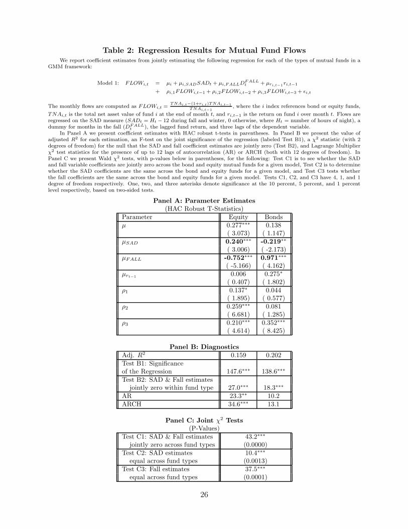
Table 2: Regression Results for Mutual Fund FlowsWe report coefficient estimates from jointly estimating the following regression for each of the types of mutual funds in a

GMM framework:

Model 1: FLOWi,t = μi + μi,SADSADt + μi,F ALLDF ALLt + μri,t−1ri,t−1

+ ρi,1FLOWi,t−1 + ρi,2FLOWi,t−2 + ρi,3FLOWi,t−3 + εi,t

The monthly flows are computed as FLOWi,t =TNAi,t−(1+ri,t)TNAi,t−1

TNAi,t−1, where the i index references bond or equity funds,

TNAi,t is the total net asset value of fund i at the end of month t, and ri,t−1 is the return on fund i over month t. Flows areregressed on the SAD measure (SADt = Ht − 12 during fall and winter, 0 otherwise, where Ht = number of hours of night), adummy for months in the fall (DF ALL

t ), the lagged fund return, and three lags of the dependent variable.In Panel A we present coefficient estimates with HAC robust t-tests in parentheses. In Panel B we present the value of

adjusted R2 for each estimation, an F-test on the joint significance of the regression (labeled Test B1), a χ2 statistic (with 2degrees of freedom) for the null that the SAD and fall coefficient estimates are jointly zero (Test B2), and Lagrange Multiplierχ2 test statistics for the presence of up to 12 lags of autocorrelation (AR) or ARCH (both with 12 degrees of freedom). InPanel C we present Wald χ2 tests, with p-values below in parentheses, for the following: Test C1 is to see whether the SADand fall variable coefficients are jointly zero across the bond and equity mutual funds for a given model, Test C2 is to determinewhether the SAD coefficients are the same across the bond and equity funds for a given model, and Test C3 tests whetherthe fall coefficients are the same across the bond and equity funds for a given model. Tests C1, C2, and C3 have 4, 1, and 1degree of freedom respectively. One, two, and three asterisks denote significance at the 10 percent, 5 percent, and 1 percentlevel respectively, based on two-sided tests.

Panel A: Parameter Estimates(HAC Robust T-Statistics)

Parameter Equity Bondsμ 0.277∗∗∗ 0.138

( 3.073) ( 1.147)μSAD 0.240∗∗∗ -0.219∗∗

( 3.006) ( -2.173)μFALL -0.752∗∗∗ 0.971∗∗∗

( -5.166) ( 4.162)μrt−1 0.006 0.275∗

( 0.407) ( 1.802)ρ1 0.137∗ 0.044

( 1.895) ( 0.577)ρ2 0.259∗∗∗ 0.081

( 6.681) ( 1.285)ρ3 0.210∗∗∗ 0.352∗∗∗

( 4.614) ( 8.425)

Panel B: DiagnosticsAdj. R2 0.159 0.202Test B1: Significanceof the Regression 147.6∗∗∗ 138.6∗∗∗

Test B2: SAD & Fall estimatesjointly zero within fund type 27.0∗∗∗ 18.3∗∗∗

AR 23.3∗∗ 10.2ARCH 34.6∗∗∗ 13.1

Panel C: Joint χ2 Tests(P-Values)

Test C1: SAD & Fall estimates 43.2∗∗∗

jointly zero across fund types (0.0000)Test C2: SAD estimates 10.4∗∗∗

equal across fund types (0.0013)Test C3: Fall estimates 37.5∗∗∗

equal across fund types (0.0001)

26

Table 3: Economic Magnitude of Mutual Fund Flowsbased on Coefficient Estimates from Table 2

We translate the SAD and fall coefficient estimates from Table 2 into economically meaningful values based on the December2002 aggregate value of the equity mutual funds we consider ($1.16 trillion) and the bond mutual funds we consider ($809 billion).The first value presented in each cell is the percentage mutual fund flow that can be attributed to the variable(s) specifiedin the column header, and the second value in each cell, in parentheses, is the economic equivalent of the percentage flow inreference to the aggregate value of the funds we consider. Panel A reports equity mutual fund flows and bond funds flows areshown in Panel B.

Panel A: Equity Mutual Fund Flows:Marginal Effect of Marginal Effect of Total Net Effect of Both

Month Fall Variable: SAD Variable: Fall and SAD Variables:% Flows ($ Flows) % Flows ($ Flows) % Flows ($ Flows)

October -0.752 (-$8.72 billion) 0.274 ($3.17 billion) -0.478 (- $5.55 billion)November -0.752 (-$8.72 billion) 0.571 ($6.63 billion) -0.181 (- $2.10 billion)December -0.752 (-$8.72 billion) 0.706 ($8.18 billion) -0.046 (- $0.53 billion)January 0 ($0) 0.624 ($7.24 billion) 0.624 ($7.24 billion)February 0 ($0) 0.365 ($4.24 billion) 0.365 ($4.24 billion)March 0 ($0) 0.031 ($0.36 billion) 0.031 ($0.36 billion)

Panel B: Bond Mutual Fund FlowsMarginal Effect of Marginal Effect of Total Net Effect of Both

Month Fall Variable: SAD Variable: Fall and SAD Variables:% Flows ($ Flows) % Flows ($ Flows) % Flows ($ Flows)

October 0.971 ($7.86 billion) -0.250 (-$2.02 billion) 0.721 ($5.83 billion)November 0.971 ($7.86 billion) -0.521 (-$4.22 billion) 0.450 ($3.64 billion)December 0.971 ($7.86 billion) -0.644 (-$5.21 billion) 0.327 ($2.65 billion)January 0 ($0) -0.570 (-$4.61 billion) -0.570 (-$4.61 billion)February 0 ($0) -0.333 (-$2.69 billion) -0.333 (-$2.69 billion)March 0 ($0) -0.028 (-$0.23 billion) -0.028 (-$0.23 billion)

27

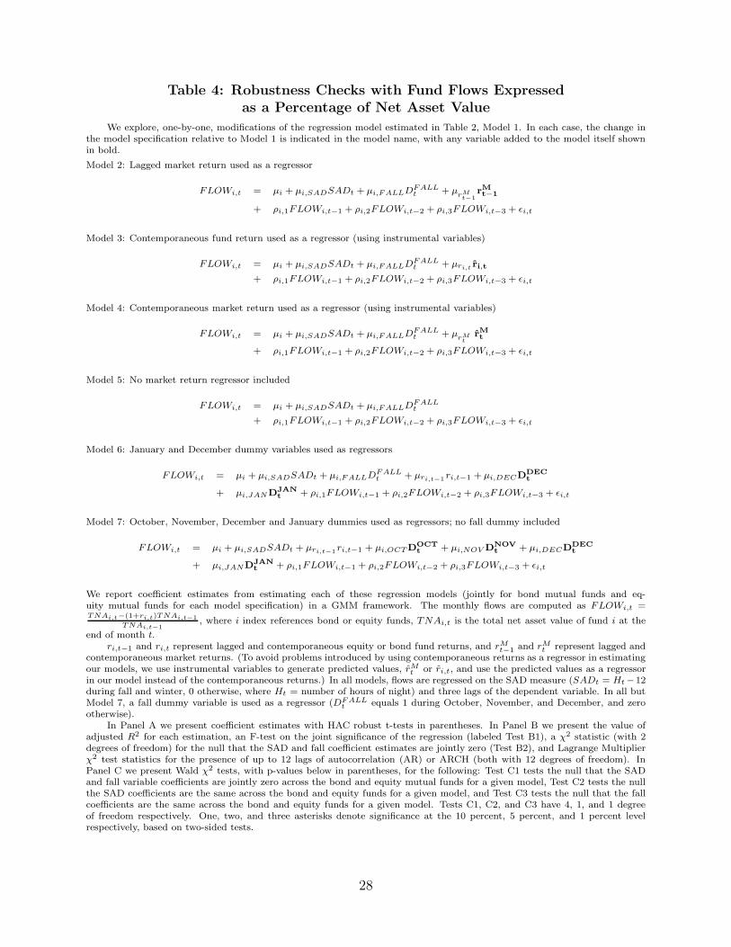
Table 4: Robustness Checks with Fund Flows Expressedas a Percentage of Net Asset Value

We explore, one-by-one, modifications of the regression model estimated in Table 2, Model 1. In each case, the change inthe model specification relative to Model 1 is indicated in the model name, with any variable added to the model itself shownin bold.

Model 2: Lagged market return used as a regressor

FLOWi,t = μi + μi,SADSADt + μi,F ALLDF ALLt + μrM

t−1rMt−1

+ ρi,1FLOWi,t−1 + ρi,2FLOWi,t−2 + ρi,3FLOWi,t−3 + εi,t

Model 3: Contemporaneous fund return used as a regressor (using instrumental variables)

FLOWi,t = μi + μi,SADSADt + μi,F ALLDF ALLt + μri,t ri,t

+ ρi,1FLOWi,t−1 + ρi,2FLOWi,t−2 + ρi,3FLOWi,t−3 + εi,t

Model 4: Contemporaneous market return used as a regressor (using instrumental variables)

FLOWi,t = μi + μi,SADSADt + μi,F ALLDF ALLt + μrM

trMt

+ ρi,1FLOWi,t−1 + ρi,2FLOWi,t−2 + ρi,3FLOWi,t−3 + εi,t

Model 5: No market return regressor included

FLOWi,t = μi + μi,SADSADt + μi,F ALLDF ALLt

+ ρi,1FLOWi,t−1 + ρi,2FLOWi,t−2 + ρi,3FLOWi,t−3 + εi,t

Model 6: January and December dummy variables used as regressors

FLOWi,t = μi + μi,SADSADt + μi,F ALLDF ALLt + μri,t−1 ri,t−1 + μi,DECDDEC

t

+ μi,JANDJANt + ρi,1FLOWi,t−1 + ρi,2FLOWi,t−2 + ρi,3FLOWi,t−3 + εi,t

Model 7: October, November, December and January dummies used as regressors; no fall dummy included

FLOWi,t = μi + μi,SADSADt + μri,t−1ri,t−1 + μi,OCT DOCTt + μi,NOV DNOV

t + μi,DECDDECt

+ μi,JANDJANt + ρi,1FLOWi,t−1 + ρi,2FLOWi,t−2 + ρi,3FLOWi,t−3 + εi,t

We report coefficient estimates from estimating each of these regression models (jointly for bond mutual funds and eq-uity mutual funds for each model specification) in a GMM framework. The monthly flows are computed as FLOWi,t =TNAi,t−(1+ri,t)TNAi,t−1

TNAi,t−1, where i index references bond or equity funds, TNAi,t is the total net asset value of fund i at the

end of month t.ri,t−1 and ri,t represent lagged and contemporaneous equity or bond fund returns, and rM

t−1 and rMt represent lagged and

contemporaneous market returns. (To avoid problems introduced by using contemporaneous returns as a regressor in estimatingour models, we use instrumental variables to generate predicted values, rM

t or ri,t, and use the predicted values as a regressorin our model instead of the contemporaneous returns.) In all models, flows are regressed on the SAD measure (SADt = Ht −12during fall and winter, 0 otherwise, where Ht = number of hours of night) and three lags of the dependent variable. In all butModel 7, a fall dummy variable is used as a regressor (DF ALL

t equals 1 during October, November, and December, and zerootherwise).

In Panel A we present coefficient estimates with HAC robust t-tests in parentheses. In Panel B we present the value ofadjusted R2 for each estimation, an F-test on the joint significance of the regression (labeled Test B1), a χ2 statistic (with 2degrees of freedom) for the null that the SAD and fall coefficient estimates are jointly zero (Test B2), and Lagrange Multiplierχ2 test statistics for the presence of up to 12 lags of autocorrelation (AR) or ARCH (both with 12 degrees of freedom). InPanel C we present Wald χ2 tests, with p-values below in parentheses, for the following: Test C1 tests the null that the SADand fall variable coefficients are jointly zero across the bond and equity mutual funds for a given model, Test C2 tests the nullthe SAD coefficients are the same across the bond and equity funds for a given model, and Test C3 tests the null that the fallcoefficients are the same across the bond and equity funds for a given model. Tests C1, C2, and C3 have 4, 1, and 1 degreeof freedom respectively. One, two, and three asterisks denote significance at the 10 percent, 5 percent, and 1 percent levelrespectively, based on two-sided tests.

28

Table 5: Robustness Checks with Fund Flows Expressedas a Percentage of Lagged Total Market Capitalization

We explore modifications of the regression model estimated in Table 2, Model 1. The first change, affecting all modelsestimated in the table, is to the dependent variable. While Table 4 examined flows as a percentage of total net asset value ofthe fund, in this table we examine flows as a percentage of total market capitalization:

FLOW ∗i,t =

TNAi,t − (1 + ri,t)TNAi,t−1

MKTt−1(4)

The index i references bond or equity funds, TNAi,t is the total net asset value of fund i at the end of month t, ri,t is thereturn on fund i over period t, and MKTt−1 is the lagged total market value of NYSE, AMEX, and NASDAQ.

Changes in each model specification relative to Model 1 are indicated in the model name, with any variable added to themodel itself shown in bold.

Model 1∗: FLOW ∗ is dependent variable

FLOW ∗i,t = μi + μi,SADSADt + μi,F ALLDF ALL

t + μri,t−1 ri,t−1

+ ρi,1FLOW ∗i,t−1 + ρi,2FLOW ∗

i,t−2 + ρi,3FLOW ∗i,t−3 + εi,t

Model 2∗: FLOW ∗ is dependent variable and lagged market return used as a regressor

FLOW ∗i,t = μi + μi,SADSADt + μi,F ALLDF ALL

t + μrMt−1

rMt−1

+ ρi,1FLOW ∗i,t−1 + ρi,2FLOW ∗

i,t−2 + ρi,3FLOW ∗i,t−3 + εi,t

Model 3∗: FLOW ∗ is dependent variable and contemporaneous fund return used as a regressor (using instrumental variables)

FLOW ∗i,t = μi + μi,SADSADt + μi,F ALLDF ALL

t + μri,t ri,t

+ ρi,1FLOW ∗i,t−1 + ρi,2FLOW ∗

i,t−2 + ρi,3FLOW ∗i,t−3 + εi,t

Model 4∗: FLOW ∗ is dependent variable and contemporaneous market return used as a regressor (using instrumental variables)

FLOW ∗i,t = μi + μi,SADSADt + μi,F ALLDF ALL

t + μrMt

rMt

+ ρi,1FLOW ∗i,t−1 + ρi,2FLOW ∗

i,t−2 + ρi,3FLOW ∗i,t−3 + εi,t

Model 5∗: FLOW ∗ is dependent variable and no market return regressor included

FLOW ∗i,t = μi + μi,SADSADt + μi,F ALLDF ALL

t

+ ρi,1FLOW ∗i,t−1 + ρi,2FLOW ∗

i,t−2 + ρi,3FLOW ∗i,t−3 + εi,t

Model 6∗: FLOW ∗ is dependent variable and January and December dummy variables used as regressors

FLOW ∗i,t = μi + μi,SADSADt + μi,F ALLDF ALL

t + μri,t−1 ri,t−1 + μi,DECDDECt

+ μi,JANDJANt + ρi,1FLOW ∗

i,t−1 + ρi,2FLOW ∗i,t−2 + ρi,3FLOW ∗

i,t−3 + εi,t

Model 7∗: FLOW ∗ is dependent variable; October, November, December and January dummies used as regressors; no falldummy included

FLOW ∗i,t = μi + μi,SADSADt + μri,t−1ri,t−1 + μi,OCT DOCT

t + μi,NOV DNOVt + μi,DECDDEC

t

+ μi,JANDJANt + ρi,1FLOW ∗

i,t−1 + ρi,2FLOW ∗i,t−2 + ρi,3FLOW ∗

i,t−3 + εi,t

We report coefficient estimates from estimating each of these regression models (jointly for bond mutual funds and equitymutual funds for each model specification) in a GMM framework. ri,t−1 and ri,t represent lagged and contemporaneous equityor bond fund returns, and rM

t−1 and rMt represent lagged and contemporaneous market returns. (To avoid problems introduced

by using contemporaneous returns as a regressor in estimating our models, we use instrumental variables to generate predictedvalues, rM

t or ri,t, and use the predicted values as a regressor in our model instead of the contemporaneous returns.) In allmodels, flows are regressed on the SAD measure (SADt = Ht − 12 during fall and winter, 0 otherwise, where Ht = numberof hours of night) and three lags of the dependent variable. In all but Model 7, a fall dummy variable is used as a regressor(DF ALL

t equals 1 during October, November, and December, and zero otherwise).In Panel A we present coefficient estimates with HAC robust t-tests in parentheses. In Panel B we present the value of

adjusted R2 for each estimation, an F-test on the joint significance of the regression (labeled Test B1), a χ2 statistic (with 2degrees of freedom) for the null that the SAD and fall coefficient estimates are jointly zero (Test B2), and Lagrange Multiplierχ2 test statistics for the presence of up to 12 lags of autocorrelation (AR) or ARCH (both with 12 degrees of freedom). InPanel C we present Wald χ2 tests, with p-values below in parentheses, for the following: Test C1 tests the null that the SADand fall variable coefficients are jointly zero across the bond and equity mutual funds for a given model, Test C2 tests the nullthe SAD coefficients are the same across the bond and equity funds for a given model, and Test C3 tests the null that the fallcoefficients are the same across the bond and equity funds for a given model. Tests C1, C2, and C3 have 4, 1, and 1 degreeof freedom respectively. One, two, and three asterisks denote significance at the 10 percent, 5 percent, and 1 percent levelrespectively, based on two-sided tests.

PanelA

:Param

ete

rEst

imate

s(H

AC

Robust

T-S

tati

stic

s)M

odel

2M

odel

3M

odel

4M

odel

5M

odel

6M

odel

7E

quity

Bonds

Equity

Bonds

Equity

Bonds

Equity

Bonds

Equity

Bonds

Equity

Bonds

μ0.2

85∗∗

∗0.2

59∗∗

0.4

18∗∗

∗−1

.957∗∗

∗0.3

91∗∗

∗0.1

47

0.2

81∗∗

∗0.2

38∗∗

0.2

50∗∗

∗0.1

14

0.1

93∗∗

0.1

26

(3.1

36)

(2.1

53)

(6.4

03)

(-7

.661)

(4.2

38)

(1.0

45)

(3.0

86)

(2.1

07)

(2.9

08)

(0.9

79)

(2.4

02)

(1.0

10)

μS

AD

0.2

29∗∗

∗-0

.199∗

0.2

87∗∗

∗-0

.135∗∗

∗0.2

97∗∗

∗-0

.214∗∗

∗0.2

48∗∗

∗-0

.200∗

0.3

56∗∗

-0.1

69

0.6

68∗∗

∗-0

.175

(2.7

07)

(-1

.890)

(11.3

62)

(-3

.892)

(5.5

49)

(-3

.571)

(3.0

32)

(-1

.934)

(2.2

02)

(-1

.007)

(3.9

76)

(-0

.751)

μF

AL

L-0

.758∗∗

∗0.9

15∗∗

∗-0

.806∗∗

∗0.9

16∗∗

∗-0

.831∗∗

∗0.9

78∗∗

∗-0

.784∗∗

∗0.9

28∗∗

∗-0

.644∗∗

∗0.7

12∗∗

..

(-4

.454)

(3.5

73)

(-1

4.8

5)

(10.4

39)

(-7

.309)

(6.2

12)

(-

4.8

72)

(3.7

83)

(-2

.596)

(2.4

06)

..

μr

t−

1.

..

..

..

.0.0

03

0.2

93∗

−0.0

01

0.2

91∗

..

..

..

..

(0.2

19)

(1.8

84)

(-0

.071)

(1.8

79)

μr

M t−

10.0

21∗

−0.0

06

..

..

..

..

..

(1.7

16)

(-0

.271)

..

..

..

..

..

μr

t.

.−0

.082

5.0

63∗∗

∗.

..

..

..

..

.(

-1.0

17)

(7.9

63)

..

..

..

..

μr

M t.

..

.−0

.041

0.0

52

..

..

..

..

..

(-0

.532)

(0.3

63)

..

..

..

μO

CT

..

..

..

..

..

−0.6

72∗∗

∗0.6

84∗∗

..

..

..

..

..

(-3

.052)

(2.3

74)

μN

OV

..

..

..

..

..

−1.6

58∗∗

∗0.8

78∗

..

..

..

..

..

(-4

.460)

(1.6

97)

μD

EC

..

..

..

..

−0.9

03∗∗

∗0.5

59∗

−2.4

23∗∗

∗1.3

75∗∗

..

..

..

..

(-4

.039)

(1.7

68)

(-5

.294)

(2.1

65)

μJ

AN

..

..

..

..

−0.0

15

−0.3

50

−0.8

17

−0.4

65

..

..

..

..

(-0

.030)

(-0

.619)

(-1

.581)

(-0

.643)

ρ1

0.1

11

0.0

73

0.0

37∗∗

−0.0

66∗∗

0.0

51∗

0.0

19

0.1

38∗

0.0

79

0.0

83

0.0

07

0.0

33

−0.0

00

(1.4

25)

(0.9

76)

(2.1

20)

(-2

.150)

(1.8

47)

(0.3

78)

(1.9

27)

(1.0

54)

(1.0

03)

(0.0

92)

(0.3

98)

(-0

.004)

ρ2

0.2

62∗∗

∗0.0

77

0.2

47∗∗

∗−0

.068∗∗

0.2

58∗∗

∗0.0

14

0.2

66∗∗

∗0.0

76

0.2

77∗∗

∗0.0

38

0.3

01∗∗

∗0.0

45

(6.1

24)

(1.1

68)

(28.1

76)

(-2

.083)

(13.0

52)

(0.3

21)

(6.5

42)

(1.1

74)

(6.4

76)

(0.6

32)

(6.6

63)

(0.7

00)

ρ3

0.2

18∗∗

∗0.3

56∗∗

∗0.2

62∗∗

∗0.3

51∗∗

∗0.2

61∗∗

∗0.3

83∗∗

∗0.2

07∗∗

∗0.3

53∗∗

∗0.2

40∗∗

∗0.3

72∗∗

∗0.2

71∗∗

∗0.3

65∗∗

∗(

4.7

01)

(7.7

63)

(16.7

27)

(19.3

89)

(10.0

28)

(13.8

06)

(4.6

31)

(7.9

45)

(5.0

14)

(8.7

60)

(5.7

92)

(8.4

47)

PanelB

:D

iagnost

ics

Adj.

R2

0.1

69

0.1

96

0.1

63

0.3

18

0.1

62

0.1

96

0.1

68

0.2

04

0.2

07

0.2

18

0.2

37

0.2

09

Tes

tB

1124.0

∗∗∗

123.3

∗∗∗

1306.0

∗∗∗

2832.6

∗∗∗

320.3

∗∗∗

378.6

∗∗∗

122.6

∗∗∗

125.0

∗∗∗

219.3

∗∗∗

153.7

∗∗∗

225.4

∗∗∗

166.4

∗∗∗

Tes

tB

220.0

∗∗∗

13.4

∗∗∗

225.3

∗∗∗

121.2

∗∗∗

54.0

∗∗∗

38.6

∗∗∗

23.8

∗∗∗

15.1

∗∗∗

6.7

∗∗9.3

∗∗∗

..

AR

23.7

∗∗11.2

19.9

∗12.4

20.3

∗12.6

22.0

∗∗10.5

20.9

∗15.8

16.2

15

AR

CH

38.4

∗∗∗

13.6

41.3

∗∗∗

10.5

39.8

∗∗∗

13.6

32.3

∗∗∗

13.5

37.4

∗∗∗

12.9

35.7

∗∗∗

13.3

PanelC

:Join

tχ

2Test

s(P

-valu

es)

Tes

tC

133.8

506.2

139.3

41.5

13.1

.(0

.0000)

(0.0

000)

(0.0

000)

(0.0

000)

(0.0

110)

.Tes

tC

28.6

97.9

46.3

10.3

4.4

8.4

(0.0

035)

(0.0

000)

(0.0

000)

(0.0

013)

(0.0

356)

(0.0

038)

Tes

tC

330.3

282.6

112.2

36.4

9.7

.(0

.0000)

(0.0

000)

(0.0

000)

(0.0

000)

(0.0

019)

.

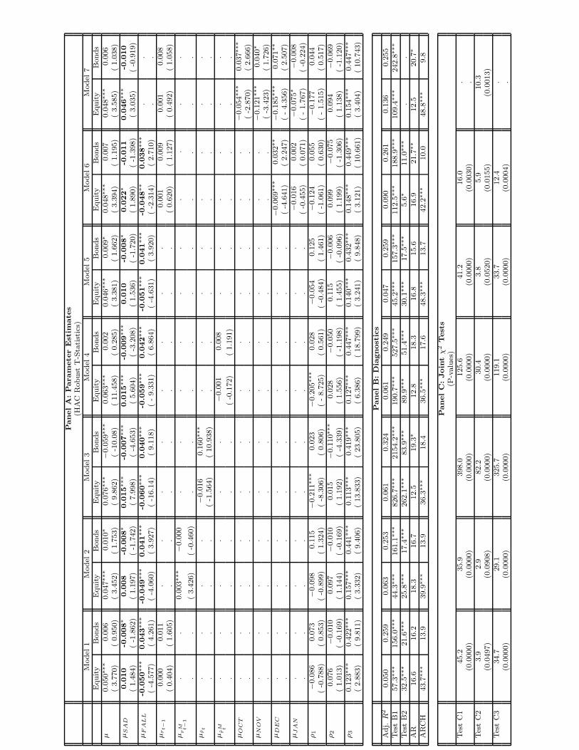
PanelA

:Param

ete

rEst

imate

s(H

AC

Robust

T-S

tati

stic

s)M

odel

1M

odel

2M

odel

3M

odel

4M

odel

5M

odel

6M

odel

7E

quity

Bonds

Equity

Bonds

Equity

Bonds

Equity

Bonds

Equity

Bonds

Equity

Bonds

Equity

Bonds

μ0.0

50∗∗

∗0.0

06

0.0

47∗∗

∗0.0

10∗

0.0

76∗∗

∗−0

.059∗∗

∗0.0

63∗∗

∗0.0

02

0.0

46∗∗

∗0.0

09∗

0.0

48∗∗

∗0.0

07

0.0

48∗∗

∗0.0

06

(3.7

70)

(0.9

50)

(3.4

52)

(1.7

53)

(9.8

62)

(-1

0.0

8)

(11.4

58)

(0.2

85)

(3.3

81)

(1.6

62)

(3.3

94)

(1.1

95)

(3.5

85)

(1.0

38)

μS

AD

0.0

10

-0.0

08∗

0.0

08

-0.0

08∗

0.0

15∗∗

∗-0

.007∗∗

∗0.0

15∗∗

∗-0

.009∗∗

∗0.0

10

-0.0

08∗

0.0

22∗

-0.0

11

0.0

46∗∗

∗-0

.010

(1.4

84)

(-1

.862)

(1.1

97)

(-1

.742)

(7.9

98)

(-4

.653)

(5.6

04)

(-3

.208)

(1.5

36)

(-1

.720)

(1.8

90)

(-1

.398)

(3.0

35)

(-0

.919)

μF

AL

L-0

.050∗∗

∗0.0

43∗∗

∗-0

.049∗∗

∗0.0

41∗∗

∗-0

.060∗∗

∗0.0

40∗∗

∗-0

.059∗∗

∗0.0

42∗∗

∗-0

.051∗∗

∗0.0

41∗∗

∗-0

.048∗∗

0.0

38∗∗

∗.

.(

-4.5

77)

(4.2

61)

(-4

.060)

(3.9

27)

(-1

6.1

4)

(9.1

18)

(-

9.3

31)

(6.8

64)

(-4

.631)

(3.9

20)

(-2

.314)

(2.7

10)

..

μr

t−

10.0

00

0.0

11

..

..

..

..

0.0

01

0.0

09

0.0

01

0.0

08

(0.4

04)

(1.6

05)

..

..

..

..

(0.6

20)

(1.1

27)

(0.4

92)

(1.0

58)

μr

M t−

1.

.0.0

03∗∗

∗−0

.000

..

..

..

..

..

..

(3.4

26)

(-0

.460)

..

..

..

..

..

μr

t.

..

.−0

.016

0.1

60∗∗

∗.

..

..

..

..

..

.(

-1.5

64)

(10.9

38)

..

..

..

..

μr

M t.

..

..

.−0

.001

0.0

08

..

..

..

..

..

..

(-0

.172)

(1.1

91)

..

..

..

μO

CT

..

..

..

..

..

..

−0.0

54∗∗

∗0.0

37∗∗

∗.

..

..

..

..

..

.(

-2.8

70)

(2.6

66)

μN

OV

..

..

..

..

..

..

−0.1

21∗∗

∗0.0

40∗

..

..

..

..

..

..

(-3

.423)

(1.7

26)

μD

EC

..

..

..

..

..

−0.0

69∗∗

∗0.0

32∗∗

−0.1

85∗∗

∗0.0

71∗∗

..

..

..

..

..

(-4

.641)

(2.2

47)

(-

4.3

56)

(2.5

07)

μJ

AN

..

..

..

..

..

−0.0

16

0.0

02

−0.0

75∗

−0.0

08

..

..

..

..

..

(-0

.455)

(0.0

71)

(-

1.7

67)

(-0

.224)

ρ1

−0.0

86

0.0

73

−0.0

98

0.1

15

−0.2

11∗∗

∗0.0

23

−0.2

05∗∗

∗0.0

28

−0.0

54

0.1

25

−0.1

24

0.0

55

−0.1

77

0.0

44

(-0

.788)

(0.8

53)

(-0

.899)

(1.3

24)

(-8

.306)

(0.8

06)

(-

8.7

25)

(0.5

61)

(-0

.484)

(1.4

61)

(-1

.061)

(0.6

30)

(-

1.5

15)

(0.5

17)

ρ2

0.0

76

−0.0

10

0.0

97

−0.0

10

0.0

15

−0.1

10∗∗

∗0.0

28

−0.0

50

0.1

15

−0.0

06

0.0

99

−0.0

75

0.0

94

−0.0

69

(1.0

13)

(-0

.169)

(1.1

44)

(-0

.169)

(1.1

92)

(-4

.339)

(1.5

56)

(-1

.198)

(1.4

55)

(-0

.096)

(1.1

99)

(-1

.306)

(1.1

38)

(-1

.120)

ρ3

0.1

23∗∗

∗0.4

22∗∗

∗0.1

57∗∗

∗0.4

41∗∗

∗0.1

13∗∗

∗0.4

19∗∗

∗0.1

27∗∗

∗0.4

47∗∗

∗0.1

40∗∗

∗0.4

32∗∗

∗0.1

48∗∗

∗0.4

49∗∗

∗0.1

54∗∗

∗0.4

47∗∗

∗(

2.8

83)

(9.8

11)

(3.3

32)

(9.4

06)

(13.8

33)

(23.8

05)

(6.3

86)

(18.7

99)

(3.2

41)

(9.8

48)

(3.1

21)

(10.6

61)

(3.4

04)

(10.7

43)

PanelB

:D

iagnost

ics

Adj.

R2

0.0

50

0.2

59

0.0

63

0.2

53

0.0

61

0.3

24

0.0

61

0.2

49

0.0

47

0.2

59

0.0

90

0.2

61

0.1

36

0.2

55

Tes

tB

157.3

∗∗∗

156.0

∗∗∗

44.3

∗∗∗

161.1

∗∗∗

826.7

∗∗∗

2154.2

∗∗∗

190.7

∗∗∗

527.5

∗∗∗

45.2

∗∗∗

157.3

∗∗∗

112.5

∗∗∗

188.9

∗∗∗

109.4

∗∗∗

242.8

∗∗∗

Tes

tB

232.5

∗∗∗

21.6

∗∗∗

25.8

∗∗∗

17.4

∗∗∗

262.1

∗∗∗

83.9

∗∗∗

89.9

∗∗∗

51.4

∗∗∗

30.1

∗∗∗

17.5

∗∗∗

5.6

∗11.0

∗∗∗

..

AR

16.6

16.2

18.3

16.7

12.5

19.3

∗12.8

18.3

16.8

15.6

16.9

21.7

∗∗12.5

20.7

∗A

RC

H43.7

∗∗∗

13.9

39.9

∗∗∗

13.9

36.3

∗∗∗

18.4

36.5

∗∗∗

17.6

48.3

∗∗∗

13.7

42.2

∗∗∗

10.0

48.8

∗∗∗

9.8

PanelC

:Join

tχ

2Test

s(P

-valu

es)

Tes

tC

145.2

35.9

398.0

125.6

41.2

16.0

.(0

.0000)

(0.0

000)

(0.0

000)

(0.0

000)

(0.0

000)

(0.0

030)

.Tes

tC

23.9

2.9

82.2

30.4

3.8

5.9

10.3

(0.0

497)

(0.0

908)

(0.0

000)

(0.0

000)

(0.0

520)

(0.0

155)

(0.0

013)

Tes

tC

334.7

29.1

325.7

119.1

33.7

12.4

.(0

.0000)

(0.0

000)

(0.0

000)

(0.0

000)

(0.0

000)

(0.0

004)

.

Figure 1:

Average Monthly Equity and Bond Fund FlowsPercentage of Last Period Total Market Value, Deviation from Mean

Deviations of average monthly flows from average annual flows for bond mutual fundsand equity mutual funds. The flows upon which the averages are based are computed as apercentage of the prior period’s aggregate market value for the appropriate fund. We use data forequity funds and bond funds provided by CRSP over January 1992 through December 2002.