searching for wages in an estimated labor matching...
TRANSCRIPT

Searching for Wages in an Estimated Labor
Matching Model∗
Ryan Chahrour†
Boston College
Sanjay K. Chugh‡
Ohio State University
Kiel Institute
Tristan Potter§
Drexel University
March 12, 2018
Abstract
We estimate a real business cycle economy with search frictions in the labor market
in which the latent wage follows a non-structural ARMA process. The estimated model
does an excellent job matching a broad set of quantity data and wage indicators. Under
the estimated process, wages respond immediately to shocks but converge slowly to
their long-run levels, inducing substantial variation in labor’s share of surplus. These
results are not consistent with either a rigid real wage or flexible Nash bargaining.
Despite inducing a strong endogenous response of wages, neutral shocks to productivity
account for the vast majority of aggregate fluctuations in the economy, including labor
market variables.
Keywords: Search and Matching, Wages, Unemployment, Business Cycles
JEL Classification: E32, E24
∗We thank Susanto Basu, Fabio Schiantarelli, John Seater, Rosen Valchev, and seminar participantsat Boston College, Boston University, CREI, the Society for Economic Dynamics Meetings (2017), theEconometric Society North American Summer meetings (2017), the Toulouse School of Economics, andSimon Fraser University for many helpful comments and suggestions.†Department of Economics, Boston College, Chestnut Hill, MA 02467. Telephone: 617-552-0902. Email:
[email protected].‡Department of Economics, Ohio State University, Columbus, OH 43210. Telephone: 614-247-8718.
Email: [email protected].§School of Economics, LeBow College of Business, Drexel University, Philadelphia, PA 19104. Telephone:
215-895-2540. Email: [email protected].

1 Introduction
Over the past decade, researchers have debated the theoretical and empirical merits of al-
ternative structural models of wage determination in labor search and matching models.
This paper steps back from that debate, initiated by Shimer (2005) and Hall (2005), and
instead asks: What properties of a generic wage-determination process are needed to match
the historical comovements of output, consumption, investment, unemployment, labor-force
participation, and job creation in the US? To answer this question, we estimate a search and
matching model that is structural in every way except for the determination of wages, which
we link to the fundamental shocks in the economy via a non-structural ARMA process. Be-
cause we do not take an a priori stance on how wages are determined, our specification nests
a variety of possible structural models of wage determination. Estimation of the model de-
livers a striking result: The estimated wage process is not consistent with either a rigid real
wage or Nash bargaining, yet productivity shocks account for the vast majority of aggregate
fluctuations in the economy, including labor market variables and observed wage measures.
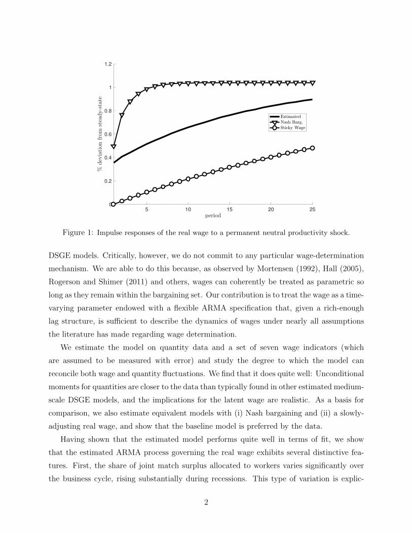
Figure 1 depicts the response of our estimated wage process to a permanent neutral pro-
ductivity shock, which our estimation determines is the principal driver of business cycles.1
The impact response of the wage to a productivity shock is nearly as large as under Nash
bargaining, inconsistent with most models of real wage rigidity. However, while the Nash
wage continues to rise in the periods just after the shock, the estimated wage approaches
its new long-run level only gradually, with full adjustment taking several years. This combi-
nation of a strong impact response, but slow convergence—accommodated by our agnostic
approach to modeling wages—is the key feature that allows productivity shocks to simultane-
ously match the empirical properties of real quantities, labor market variables, and observed
wage measures. Our results thus provide new guidance in the ongoing search for structural
foundations of wage determination and offer strong support for technology as an important
driver of business cycle fluctuations.
We estimate a real dynamic stochastic general equilibrium (DSGE) model, endowed with
external habit formation, adjustment costs in investment, variable capital utilization, and
search and matching frictions in the labor market. More or less complicated versions of this
basic model underlie the vast majority of the recent literature on structural estimation of
1In addition to permanent total factor productivity, our model allows for fundamental shocks toinvestment-specific technology, labor supply, government spending, labor tax rates, and a non-fundamentalshock directly impacting only wages.
1
5 10 15 20 25
0
0.2
0.4
0.6
0.8
1
1.2
Figure 1: Impulse responses of the real wage to a permanent neutral productivity shock.
DSGE models. Critically, however, we do not commit to any particular wage-determination
mechanism. We are able to do this because, as observed by Mortensen (1992), Hall (2005),
Rogerson and Shimer (2011) and others, wages can coherently be treated as parametric so
long as they remain within the bargaining set. Our contribution is to treat the wage as a time-
varying parameter endowed with a flexible ARMA specification that, given a rich-enough
lag structure, is sufficient to describe the dynamics of wages under nearly all assumptions
the literature has made regarding wage determination.
We estimate the model on quantity data and a set of seven wage indicators (which
are assumed to be measured with error) and study the degree to which the model can
reconcile both wage and quantity fluctuations. We find that it does quite well: Unconditional
moments for quantities are closer to the data than typically found in other estimated medium-
scale DSGE models, and the implications for the latent wage are realistic. As a basis for
comparison, we also estimate equivalent models with (i) Nash bargaining and (ii) a slowly-
adjusting real wage, and show that the baseline model is preferred by the data.
Having shown that the estimated model performs quite well in terms of fit, we show
that the estimated ARMA process governing the real wage exhibits several distinctive fea-
tures. First, the share of joint match surplus allocated to workers varies significantly over
the business cycle, rising substantially during recessions. This type of variation is explic-
2

itly precluded by constant-share Nash bargaining. Second, the estimated wage process is
remarkably flexible in certain respects. In particular, wages respond strongly on impact to
permanent productivity shocks, but adjust slowly to their long-run level. Responses to other
shocks, including investment-specific technology, labor supply, and government spending also
exhibit strong impact effects followed by gradual reversion to long-run levels. There is little
in our estimation to suggest that the data call for hump-shaped responses to shocks.2
Given the apparent flexibility of wages, our model has a surprising implication regarding
the sources of business cycles: the vast majority of variation in both standard aggregate quan-
tities and labor market variables is driven by productivity shocks. In particular, roughly 70
percent of the variation in output, consumption, unemployment, and vacancies is accounted
for by permanent neutral productivity shocks. This result stands in sharp contrast with
other estimated labor search and matching models, which find a much smaller role for pro-
ductivity shocks.3 Importantly, we arrive at this result despite estimating a high impact
elasticity of wages to productivity shocks and a relatively low value of non-market activity.4
The estimated process for wages is tied to seven wage indicator series via a factor struc-
ture similar to that of Boivin and Giannoni (2006): real compensation per worker, real
compensation per hour, real weekly compensation, two Employment Cost Index measures
(one that includes benefits and one that excludes benefits) and two quality-adjusted wage
series from Haefke et al. (2013a) (one for all workers and one for new hires only). Because
the correspondence of the model wage concept with the data is imperfect and because we
have little reason to prefer any single measure, we let each series load differently on the
underlying model wage and assume that each is measured with error. We tie the model
closely to the wage data, however, by imposing tight priors that each wage series does in
fact contain substantial information regarding the wage in the model. Since the wage series
have very different dynamics, no single factor can capture them all. We find that the model
prefers, by a substantial margin, the compensation per worker measure of wages. While they
have a short history and the magnitude of their fluctuation is muted, the Employment Cost
2Whether stickiness is real or nominal is not especially important, since nominal wage stickiness mattersonly to the extent that it induces a sluggishness in real wages. Both types of frictions are potentiallyencompassed by our ARMA specification of the wage process.
3Gertler et al. (2008) find that productivity shocks explain roughly one third of the variation in the growthrate of output, and less than half of labor market outcomes. Lubik (2009) finds that productivity shocks arecritical for explaining output, but do not explain any of the variation in unemployment and vacancies.
4Hall (2005) generates volatility in unemployment by dispensing with Nash bargaining and assumingwages are inelastic with respect to productivity. Hagedorn and Manovskii (2008) achieve a similar effectunder Nash bargaining by assuming that workers have low bargaining power and that their outside optionis very close to the bargained wage. We estimate a replacement rate of roughly 25 percent.
3

Index measures also do a good job capturing the cyclical patterns of our estimated wage
process.
This paper contributes to a growing empirical literature on equilibrium search and match-
ing models of the labor market based on the seminal work of Diamond (1982), Mortensen
(1982), and Pissarides (1985). Early contributions include Mortensen and Pissarides (1994),
Merz (1995), and Andolfatto (1996). Following the Shimer (2005) critique, the literature
has modeled wage determination in many different ways. A few prominent examples include
Hall (2005), Farmer and Hollenhorst (2006), Hall and Milgrom (2008), Gertler et al. (2008),
Kennan (2010) and Christiano et al. (2016).
Parametric process for wage have also occasionally appeared in this literature. Michaillat
(2012) assumes a log-linear relationship between wages and current productivity. Our ap-
proach here builds on this work, treating the wage as a time-varying parameter that responds
dynamically — and potentially with a lag — to several fundamental shocks. Motivated by
the results of Haefke et al. (2013b), Michaillat (2012) calibrates a relatively high elasticity
of the real wage with respect to productivity shocks and finds that cyclical job rationing
leads to substantial fluctuations in unemployment. Our estimate of a large impact response
of wages to technology is consistent with his calibration. Christiano et al. (2016) also briefly
introduce a reduced-form wage process and perform an exercise similar to ours as a way to
offer support for their structural wage process. Relative to this paper, our full-information
likelihood-based approach allows us (i) to make weaker assumptions about the data ana-
logue to the model wage, and (ii) to perform the unconditional variance decomposition that
underlies our conclusion about the importance of technology shocks.
Methodologically, our approach belongs to a broader literature that integrates non-
structural components within otherwise structural models. Structural models with non-
structural blocks have been estimated by Sargent (1989), Altug (1989), Ireland (2004), and
Boivin and Giannoni (2006). The advantage of these approaches is that they allow the re-
searcher to avoid making strong structural assumptions when the a priori grounds for such
assumptions are unclear. Of course, care must be taken if such models are to be used to
analyze changes in policy, and we do not attempt to do so here. Nevertheless, we view
the methodology as a valuable strategy for identifying patterns in the data that candidate
models should match. Also related is the literature initiated by McGrattan (1994), Hall
(1996), and Chari et al. (2007), which uses dynamic models as measurement tools to infer
the non-structural “wedges” driving the economy. Cheremukhin and Restrepo-Echavarria
4

(2014) use a labor search and matching model with (variable-share) Nash bargaining in order
to examine the sources of the RBC labor wedge.
The remainder of the paper is organized as follows: Section 2 develops the model, Section
3 outlines our estimation strategy, and Section 4 describes the results and their implications
for modeling the real wage. Section 5 concludes.
2 The Model
The economy consists of a representative household and a representative firm who each
trade in markets for consumption, labor, and capital. Consumption and capital markets are
competitive, while transactions in labor markets are subject to search and matching frictions
in the spirit of Mortensen and Pissarides (1994).
2.1 Households
The representative household consists of a continuum of ex-ante identical members each of
whose unit time endowment can be allocated to working, searching for work, or leisure.5 The
household derives utility at time t from consumption and leisure (non-participation) accord-
ing to the period utility function u(ct, ft;Ct−1, ιt), where ct is household consumption, ft is
the household’s labor force participation, Ct−1 is lagged aggregate consumption capturing
the habit stock in the economy, and ιt is a preference shock shifting the marginal disutility
of labor.6 Each period, the household dedicates a portion st of its members to search for a
match in the labor market. Searching members match with probability pt, which the house-
hold takes as given. Moreover, newly-created matches become productive within the period,
so that the total labor force participation of the representative household is given by
ft = nt + (1− pt) st, (1)
where ft denotes the measure of household members in the labor force, nt denotes the measure
of currently matched workers, and (1− pt) st denotes the measure of household workers who
5Consistent with the labor search literature incorporating a participation margin, we interpret non-participation in the labor force as leisure in the representative household’s optimization problem.
6As is common in the literature, we assume external habits. Since both aggregate consumption Ct−1
and ιt are exogenous to the representative household, we suppress the dependence of u(·) on Ct−1 and ιt insubsequent expressions. Henceforth, we denote by capitalized letters aggregate counterparts to household-and firm-specific variables.
5

Period t-1 Period t+1Period t
Aggregate state
realized
nt-1 nt
Production (using nt employees and kt units
of capital), goods markets and capital
markets clear
Employment separation
occurs (ρnt-1 employees separate)
Search and matching in labor market
nt = (1-ρ)nt-1 + m(st, vt)yields
Firms post vt job
vacancies
Optimal labor-force
participation decisions: st individuals search for
jobs
(1-ρ)nt-1 individuals counted as employed, st individuals counted as searching and
unemployed
Figure 2: Timing of events in labor markets.
search but fail to find a match in period t.7 Each period, previously productive matches
dissolve with exogenous probability λ, so that the law of motion for matched workers faced
by the household is
nt = (1− λ)nt−1 + ptst. (2)
The unemployment rate in the economy is therefore given by
urt =(1− pt)st
nt + (1− pt)st. (3)
Figure 2 displays the timing of events in labor markets.
In addition to choosing its consumption and labor force participation, each period the
household must also choose a level of capacity utilization for the current capital stock and
a new level of investment subject to an investment adjustment cost as in Christiano et al.
(2005). The law of motion for the stock of capital is given by
kt+1 = (1− δ(ut))kt + it, (4)
7This timing convention is consistent with the evidence on labor market flows at quarterly frequency. SeeDavis et al. (2006).
6
where δ(ut) is the depreciation rate of the capital stock, which is an increasing and convex
function of capacity utilization, denoted ut.
The household budget constraint is given by
ct + itZt
(1 + Φ
(itit−1
))+ τt = Rtutkt + (1− τnt )Wtnt + (1− pt)stκt + dt. (5)
In equation (5), households take the rental rate of capital, the wage rate of labor, the
relative price of investment in consumption units, and benefits paid to unemployed workers
(Rt,Wt, Zt and κt respectively), as given. They also receive dt, lump-sum dividends from
firms to the household, pay τnt , an exogenous distortionary tax on labor income, and pay
τt, a lump-sum tax used to finance any exogenous stream of government expenditure and
unemployment benefits that remain unfunded after labor income tax revenue is collected. In
order to maintain balanced growth, we assume that the benefit paid to unemployed workers
gradually adjusts towards current wages,
κt = (κWt−1)φκ κ1−φκt−1 . (6)
Substituting the expression for ft in equation (1) into the utility function, the represen-
tative household’s problem may be expressed as
maxct,st,it,ut,nt,kt+1
E0
∞∑t=0
βtu(ct, nt + (1− pt)st) (7)
subject to (2), (4), (5) and (6).
The first-order conditions for investment, it, and capital next period, kt+1, are given by
µKt = uc,tZt
[1 + Φ
(itit−1
)+
(itit−1
)Φ′(
itit−1
)]− Et
βuc,t+1Zt+1
(it+1
it
)2
Φ′(it+1
it
)(8)
µKt = Et
β
[(1− δ(ut+1)
)µKt+1 + uc,t+1Rt+1ut+1
](9)
where µKt denotes the Lagrange multiplier on the law of motion for capital in (4). Equation
(8) states that the utility gain from supplying an additional unit of capital must equal the
marginal utility of current consumption, taking into consideration the costs associated with
changing the level of investment. Equation (9) states that the utility gained from taking an
7
additional unit of capital into the next period is the sum of its after-depreciation continuation
value and the utility gained from consumption of future rental income. Observe that, absent
investment adjustment costs and a utilization margin, (8) implies that µKt = uc,tZt ∀t, and
so from (9) we recover the familiar real business cycle Euler equation.
Optimality of capacity utilization requires
uc,tRt = δ′(ut)µ
Kt . (10)
Finally, after some simplification, the household’s labor force participation condition may be
expressed as
−uf,tuc,t
= pt
[(1− τnt )Wt + (1− λ)Et
Ωt,t+1
(1− pt+1
pt+1
)(−uf,t+1
uc,t+1
− κt+1
)]+ (1− pt)κt,
(11)
where Ωt,t+1 ≡ β uc,t+1
uc,t. This condition states that the utility gained from keeping one more
person out of the labor force (i.e. the marginal utility of leisure) is, at the optimum, equated
to the utility gained from sending one more person to search for a job. The utility from
joining the labor force to search, in turn, depends on the utility derived from consuming
out of the earned wage in the same period, plus the asset value of the job, both discounted
according to the exogenous job-finding probability. Note that as the matching probability
and separation rate tend to unity, equation (11) becomes the RBC labor supply condition.
2.2 Firms
The representative firm chooses labor, capital, and vacancy postings so as to maximize the
present value of real dividends, discounted according to the consumer’s stochastic discount
factor. The firm produces output with a production function of the form,
yt = F (utkt, Xtnt), (12)
where Xt is a non-stationary, labor-augmenting technology shock, with long-run growth rate
γx.
The law of motion of employed labor from the firm’s perspective is given by
nt = (1− λ)nt−1 + qtvt (13)
8

where vt denotes vacancies posted in the labor market, while qt denotes the probability of a
vacancy posting returning a match. Firm profits are given by the expression
dt = AtF (utkt, Xtnt)−Wtnt −Rtutkt − anvt. (14)
where an governs the cost of posting a vacancy.
The problem of the firm may therefore be expressed as
maxvt,nt,kt
E0
∞∑t=0
βtuc,tdt (15)
subject to (13) and (14). The first order condition for capital is given by
AtFk,t = utRt. (16)
The first-order condition for vacancies is given by µNt = an/qt and the first-order condition
for labor is given by
µNt = AtFn,t −Wt + (1− λ)Et
Ωt,t+1µNt+1
. (17)
Equation (17) constitutes the vacancy posting condition, which states that the firm optimally
posts vacancies until the marginal cost of doing so is equalized with the marginal product of
labor net of the wage bill, plus the continuation value of a match. Note that as an tends to
zero and the separation rate tends to unity, the vacancy posting condition approaches the
standard RBC labor demand condition.
2.3 Government
The government runs a balanced budget, financing an exogenous stream of aggregate pur-
chases Gt through a combination of distortionary labor taxes τnt and lump-sum tax revenues
τt net of unemployment benefit transfers to households (1 − pt)stκt. The government’s re-
source constraint is thus given by
Gt = τt + τnt Wtnt − (1− pt)stκt. (18)
9
We follow Schmitt-Grohe and Uribe (2012) in assuming that government spending consists
of a trend and stationary component
Gt = GTt G
St . (19)
The trend component gradually adjusts to restore the long-run share of government spending
in the economy,
GTt = GT
t−1
(GTt−1
g
)φg,y, (20)
while transient changes in government expenditure follow an AR(1) process, specified below.
2.4 Wages
In order to close the model, we must make an assumption regarding wage determination in
the economy. Rather than take a particular stand on the microeconomic foundations of wage
determination in frictional markets, our baseline specification builds on the observation of
Hall (2005) that prices can be treated as parameters in markets characterized by search and
matching frictions. However, instead of taking the level of wages as fixed, as do Michaillat
and Saez (2013) for example, we treat the statistical process by which wages evolve in the
economy as parametric, and it is this process that we seek to estimate.
The starting point of our exercise, therefore, is a representation of equilibrium wages as
log (Wt) = βW (L)εt. (21)
Here, βW (L) is an infinite-lag polynomial and εt potentially includes all shocks affecting the
economy. Equation (21) is generic, but in our implementation we restrict the wage process
in two ways. First, we assume that equilibrium wages are cointegrated with the stochastic
trends in the economy. This assumption is necessary in order to ensure the economy has a
balanced growth path, and is consistent with all of the wage-determination mechanisms that
we are aware of in the literature. Second, we need to assume that, when making their vacancy
posting decisions, firms take as given the eventual wage a hired worker earns. With single-
worker firms, or constant returns to scale production, there is very little loss of generality
with this assumption.8 If we could estimate the infinity of coefficients implied in βW (L),
8With multiple worker firms and decreasing returns, firms may internalize the effect on surplus, andtherefore wages, created by hiring additional workers. In some contexts this leads to an inefficiency in which
10

we would therefore directly nest the vast majority of wage-determination mechanisms that
appear in the literature. Of course, in practice, such an estimation is infeasible. In Section
3, we discuss the parametric restrictions we place on equation (21) in order to implement
our empirical strategy.
For comparison, we contrast our baseline specification of wages with two alternatives.
The first alternative we consider is the model of a “wage norm”, or sticky real wage, as
suggested by Hall (2005). Hall (2005) shows that a deterministic and commonly known
trend can easily be incorporated into the norm without changing the implications. With our
stochastic trend, the case is not quite so straightforward, since the wage norm needs to adjust
to surprise shocks at some horizon in order to stay within the bargaining set. Accordingly,
we assume that wages adjust slowly to permanent shocks according to the equation
W stickyt = c
(XtZ
α1−αt
)φh (W stickyt−1
)1−φhWw,t, (22)
where the constant c depends on the steady-state labor share of the economy, φ captures the
rate of adjustment, or error-correction, of the wage norm, and Ww,t is a stationary function
of an exogenous shock to wages so that the structural wage model need not hold exactly
in all periods.9 In the rigid-wage version of our economy, we assume φh = 0.025, or an
error-correction of 2.5 percent-per-quarter.
We also consider a version of the economy where the wage is determined by Nash bar-
gaining. Following a standard derivation (reproduced in Appendix C) the Nash-bargained
wage is given by
WNBt =
(1− η)κt + η
[AtFn,t + (1− λ)Et
Ωt,t+1pt+1µ
Nt+1
]Ww,t. (23)
This version of the model explicitly allows for a calibration of low worker bargaining power
and high outside options, which Hagedorn and Manovskii (2008) argue can address the
challenge to Nash bargaining posed by Shimer (2005). As in equation (22), we allow for
independent shocks to the wage via Ww,t, which generate exogenous fluctatuations in the
split of surplus between workers and firms.
firms hire excess labor in order to suppress marginal products and therefore all wages.9The introduction of this error term allows for the sticky wage (and Nash) models to be compared directly
with our reduced-form wage model, which also contains direct shocks to the wage. We elaborate on thispoint below.
11

2.5 Equilibrium
The number of matches formed in the labor market is governed by a constant returns match-
ing function m(Vt, St).St represents the aggregate mass of job-seekers and Vt represents the
aggregate mass of vacancies posted by firms. The probabilities of forming a match in the
labor market, which both the consumer and firm take as given, are respectively
pt =m(Vt, St)
St(24)
qt =m(Vt, St)
Vt. (25)
Substituting out the matching probability definitions in (24) and (25), equilibrium is
described by a set of allocations Ct, St, It, Nt, Vt, Kt+1, the capital rental rate Rt, the
capital utilization rate ut, and a Lagrange multiplier µKt that satisfy consumer optimality
conditions (8), (9), (10) and (11), firm optimality conditions (16) and (17), the aggregate
laws of motion for labor and capital
Nt = (1− λ)Nt−1 +m(Vt, St) (26)
Kt+1 = (1− δ(ut))Kt + It (27)
and the aggregate resource constraint
Ct + ItZt
(1 + Φ
(ItIt−1
))+Gt = AtF (utKt, XtNt)− anVt (28)
taking as given the exogenous processes for Xt, Zt, ιt, Gt, τnt , as well as the parametric wage
process described in equation (21).
3 Empirical Strategy
3.1 Functional Forms
The representative household derives utility at time t from the utility function
u(ct, ft) =
[(ct − hCt−1) · ν(ft; ιt)
]1−σ − 1
1− σ(29)
12

where h represents the degree of external habit formation with respect to last period’s ag-
gregate consumption Ct−1, and
ν(ft; ιt) = ψ(1− ft)1−ιt − 1
1− ιt(30)
where ιt controls the curvature of the disutility of labor and is allowed to vary stochasti-
cally.10 Output is produced using capital and labor according to a standard Cobb-Douglas
production function
F (utkt, Xtnt) = (utkt)α(Xtnt)
1−α. (31)
The investment adjustment cost is given by
Φ
(itit−1
)=φ
2
(itit−1
− γxγ1
α−1z
)2
(32)
so that in the steady state Φ(γxγ1
α−1z ) = Φ
′(γxγ
1α−1z ) = 0, and Φ
′′(γxγ
1α−1z ) = φ > 0.11 The
depreciation rate depends on utilization according to
δ(ut) = δ0 + δ1(ut − u) +δ2
2(ut − u)2 (33)
so that δ(u) = δ0, δ′(u) = δ1 > 0 and δ
′′(u) = δ2 > 0. Finally, we assume a standard
Cobb-Douglas matching function
m(Vt, St) = χSεtV1−εt , (34)
confirming ex post that matching probabilities remain between zero and one.
10In the log-linearized model used in estimation, shocking ι is isomorphic to shocking ψ, which is used tocalibrate the steady state.
11Our investment adjustment cost function is a special case of the form specified in Christiano et al. (2005).
13

There are five fundamental exogenous processes hitting the economy:
log(γx,t/γx) = ρx log(γx,t−1/γx) + εxt (35)
log(γz,t/γz) = ρz log(γz,t−1/γx) + εzt (36)
log(ιt/ι) = ρι log(ιt−1/ι) + ειt (37)
log(GSt ) = ρg log(GS
t−1) + εgt (38)
log(τnt ) = ρτn log(τnt−1) + ετn
t . (39)
In the above γx,t ≡ Xt/Xt−1 and γz,t ≡ Zt/Zt−1 describe the growth rates of the two stochas-
tic trends in the economy. In preliminary estimations, we consistently find ρx and ρz close
to zero, and therefore fix these equal to zero in our baseline estimation. The preferences and
technology described here are consistent with balanced growth. Since we will linearize the
economy around a steady state, we must first stationarize the first-order conditions of the
economy. The details of these steps are given in Appendix A.
3.2 A Process for Wages
Because it is not feasible to estimate the infinity of coefficients of the MA representation
of the wage in equation (21), we seek a more compact representation that spans, as much
as possible, the same set of possible dynamics for wages. A large variety of representations
is feasible, and the most appropriate one is not a priori obvious. In order to maximize the
transparency of the estimated parameters, we proceed to directly parameterize the impulse
response of wages to each shock. Formally, we assume the log of the wage evolves as the
sum of six independent components
wt = w + wx,t + wz,t + wι,t + wg,t + wτn,t + ww,t. (40)
Each term in the sum evolves according to a univariate ARMA(p, q) process, with a form that
depends on the specification of the underlying shock. For transitory shocks j ∈ ι, g, τn, w,we assume a level-stationary process,
wj,t = ρj(L)wj,t−1 + ψj(L)εj,t. (41)
14

For the non-stationary shocks, j ∈ x, z, we assume growth-stationary processes
∆wx,t = ρx(L)∆wx,t−1 + ψx(L)εx,t − φx (wx,t−1 − log(Xt−1)) (42)
∆wz,t = ρz(L)∆wz,t−1 + ψz(L)εz,t − φz(wz,t−1 −
α
α− 1log(Zt−1)
)(43)
where ∆wx,t ≡ ∆wx,t− log(γx), ∆wz,t ≡ ∆wz,t− αα−1
log(γz) and the terms multiplied by the
φj ∈ (0, 1] represent error-correction terms that ensure the level of the wage converges to a
constant ratio with the other trending variables in the economy.
Note that (40) contains an additional term, ww,t, that follows the same ARMA process as
the other terms but does not correspond to one of the fundamental shocks in the economy.
The presence of this term is important for the interpretation of our results. If this term plays
a large role in driving wages, we would conclude that the data demand large disturbances
to the wage-determination arrangement itself, and that causality in the economy runs from
wages to other labor market variables and aggregate quantities. Conversely, if our estimates
indicate that wages largely respond to the other fundamental shocks hitting the economy,
then we can conclude that the data are consistent with a strong endogenous response of
wages to economic conditions, with causality running from those fundamental shocks to
wages. As noted above, we also include this term in the rigid-wage and Nash wage processes,
thus allowing for temporary deviations from those wage-determination arrangements in our
estimated versions of those economies.
We also estimate the model using our two alternative specifications of the wage. Rear-
rangement of equation (22) shows that the slow-adjustment specification is actually nested
in our ARMA specification when φx = φz = φh and the remaining ARMA parameters are set
to zero. The Nash-wage specification is not explicitly nested in our ARMA process, and so
requires specification of an additional parameter, η, that is not present in either of our other
estimations. In order to ensure that our model comparison is not driven by prior choices on
non-nested parameters, we use the least-restrictive priors that prove feasible for parameters
related to wage determination. See Appendix D.2 for details on the prior choices.
We have also considered another natural candidate for the (stationarized) log-wage,
namely
wt = Ψxt, (44)
where xt represents the state vector, which includes both exogenous and endogenous vari-
ables. The advantage of this approach is that the endogenous states contain a summary of
15

the full history of past shocks, and in a linear combination that is by construction relevant
to the economy. This approach also directly nests many wage-determination mechanisms,
such as Nash bargaining, that do not themselves introduce additional states into the system.
This approach has drawbacks, however. First, it is hard to formulate priors on the pa-
rameter vector Ψ and, in practice, the endogeneity of some elements of xt makes it especially
difficult to constrain the Bayesian sampler (or any other search algorithm) to regions in
which equilibrium both exists and is unique. The endogenous elements of xt also mean that
it is quite difficult to characterize the restrictions implied by the representation in equation
(44) on possible dynamics for wages. These challenges notwithstanding, we have explored
representation (44) using a reliable global optimizer and found that it offers no advantage in
terms of model fit relative to the representation we adopt above.12
3.3 Data
We estimate the model using quarterly data from 1972Q1 to 2013Q4, with an additional six
years of data used to initialize the Kalman filter. We classify the data used into two groups.
The first set of observations, Y1,t, consists of real quantity indicators for which we have a
single measure. For these variables, the link between the model and data is uncontroversial,
and measurement errors are generally considered modest. Accordingly, with the exception
of output, we assume the data are a perfect measure of the corresponding model concept.
The vector Y1,t consists of log-changes in real per-capita output, consumption, investment,
and government expenditure, as well as the unemployment rate, per-capita employment, and
labor tax rates. The measurement equation linking observables with model analogues is
Y1,t =
∆ log yt
∆ log ct
∆ log it
∆ log gt
∆ log urt
∆ log nt
∆ log τnt
+
εy,t
0
0
0
0
0
0
. (45)
12The above discussion of determinacy contrasts with the common finding that exogenously specifying aprice — e.g. the interest rate in New Keynesian models — often leads to indeterminacy of equilibrium.In the labor search and matching model, the endogenous adjustment of market tightness clears markets,thereby pinning down equilibrium.
16

Table 1: Summary Moments - Data
∆y ∆c ∆i ∆g ∆ur ∆n
σ(X) 0.82 0.53 2.15 0.92 5.06 0.48σ(X)/σ(∆Y ) 1.00 0.64 2.62 1.12 6.15 0.58ρ(Xt, Xt−1) 0.35 0.46 0.47 0.17 0.66 0.62ρ(X,∆Y ) 1.00 0.62 0.74 0.23 -0.68 0.62
The covariance properties of these series are summarized in Table 1.
The inclusion of the measurement error in the output equation is necessary because the
resource constraint of the economy implies a fixed relation between output, consumption,
investment, government expenditure and vacancy postings. Since our model counterfactually
assumes balanced trade, the data do not exactly respect this relation. Nevertheless, this
measurement error is estimated to be quite small.
To these “basic” data, we then append an additional set of variables Y2,t, for which the
link to the model concepts, as well as the quality of measurement, is far less clear. In this
vector, we include two measures of vacancy postings as well as seven diverse measures of
the aggregate wage. The first measure of vacancies comes from the BLS JOLTS survey,
and is first available in 2001Q1. The second vacancy measure is given by the “Help-wanted”
advertising index produced by the Conference Board through 2009. This series demonstrates
a secular downward trend associated with the popularization of the internet and web-based
job search, so we therefore drop all observations from 2000Q1 onward. Summary statistic for
these series are included in Table 2. Given the rather different inputs into these two series,
we assume each represents a potentially rescaled version of the model concept, vt, measured
with error.
The choice of an appropriate empirical counterpart for the model wage is not obvious
for at least two reasons. First, the failure of standard measures of the wage to account for
unobserved worker heterogeneity can impart a countercyclical compositional bias upon real
wages, an issue noted by Alan Stockman and subsequently studied by Solon et al. (1994). In
recessions, unemployment should occur disproportionately among the low-skilled who earn
low wages. Average measured wages thus exhibit a countercyclical bias due to the changing
composition of the workforce, a fact that cannot be accounted for without comprehensive
individual-level data. Second, much recent literature has emphasized a distinction between
the wage of new hires in the economy and the wage of ongoing matches. In many search and
17

Table 2: Moments - Vacancy-posting Measures (Estimated Model)
JOLTS Help-Wanted Model
σ(X) 6.27 10.17 4.78σ(X)/σ(∆Y ) 7.63 12.38 5.37ρ(Xt, Xt−1) 0.49 0.68 0.59ρ(X,∆Y ) 0.38 0.78 0.78Signal Power 0.58 0.91 1.00
matching contexts it is the wage of new hires which plays the primary allocative role in the
economy.13
For the reasons cited above, we incorporate seven different real wage series in our es-
timation. The properties of these data are provided in Table 3. The first three series are
somewhat standard measures of compensation. The first is total real compensation per
worker. Given the lack of an explicit hours margin in our model, and the growing impor-
tance of non-wage compensation in the US economy, we view this as conceptually the closest
match to the real wage in our model economy. We add to this an index of compensation per
hour and real weekly compensation. These two measures are both somewhat more volatile
than our preferred measure of the wage. To address concerns about composition bias, we in-
clude four additional series: two composition-adjusted series of the Employment Cost Index
(ECI), and two quality-adjusted series from Haefke et al. (2013a). The Employment Cost
Index, compiled by the BLS, seeks to follow wages holding constant the sectoral distribution
of labor in the economy. We consider the standard ECI and the ECI adjusted to include
benefits. The quality-adjusted series, constructed by Haefke et al. (2013a), seek to adjust for
individual-level characteristics to better account for the cyclical variation in the quality of
workers. We consider their standard quality-adjusted series for all workers, as well as their
quality-adjusted series for new hires only. Several of the aforementioned series do not exist
for the full sample period, and so the wage data constitute an unbalanced panel. As with the
vacancy data, we assume each series represents a potentially rescaled version of the model
concept Wt measured with error.
13For some recent theory and empirical work on the issue see Pissarides (2009) and Kudlyak (2014), amongothers.
18

Table 3: Moments - Wage Measures (Estimated Model)
cmp/wrkr cmp/hr wkly cmp ECI ECI+ben HSV HSV-new modl
σ(X) 0.61 0.79 1.11 0.29 0.29 1.06 5.25 0.58σ(X)/σ(∆Y ) 0.74 0.96 1.35 0.35 0.35 1.29 6.39 0.65ρ(Xt, Xt−1) -0.01 -0.18 0.25 0.29 0.11 -0.12 -0.19 0.26ρ(X,∆Y ) 0.33 -0.01 0.03 0.11 0.19 0.03 -0.02 0.49Signal Power 0.28 0.16 0.13 0.39 0.41 0.13 0.01 1.00
In summary, the vector Y2,t is related to the model according to the measurement equation
Y2,t =
γv,1∆ log vt
γv,2∆ log vt
γw,1∆ logwt
γw,2∆ logwt
γw,3∆ logwt
γw,4∆ logwt
γw,5∆ logwt
γw,6∆ logwt
γw,7∆ logwt
+
εv1,t
εv2,t
εw1,t
εw2,t
εw3,t
εw4,t
εw5,t
εw6,t
εw7,t
. (46)
This approach to measurement is similar to the integration of DSGE and factor-based meth-
ods proposed by Boivin and Giannoni (2006). Further details on the data construction are
in Appendix D.2.
3.4 Identification
We log-linearize the model economy around the non-stochastic steady state and estimate it
using Bayesian methods. To do this, we first calibrate a subset of parameters according to the
values listed in Table 4. These parameters are either set to standard values, or to match long
run relationships found in the data. In particular, the compensation-to-output share µw/y
is used to pin down the long-run wage in the economy, F pins down the scaling parameter
of the disutility of labor ψ, the long-run employment rate, ur, determines the separation
parameter λ, and the long-run firm matching probability q pins down the vacancy cost an,
which is exactly neutral to dynamics in the economy.
Model dynamics are driven by shocks to five fundamental exogenous AR(1) processes:
19

Table 4: Calibrated Parameters
Parameter Concept Value
β Discount factor 0.992ι Curvature of v(·) 5.000σ Risk aversion 2.500µw/y Compensation share of output 0.700α Capital share of output 0.250q Labor matching prob., firm side 0.500ur Steady-state unempl. rate 0.062F Steady-state LFP rate 0.603δ0 Average depreciation rate 0.025δ2 Curvature of depreciation rate 0.005g/y Government share of GDP 0.205τn Steady-state labor tax rate 0.224γx Long-run TFP growth 1.002γz Long-run RPI growth 0.996
the growth rate of total factor productivity (γx,t), the growth rate of the relative price of
investment (γz,t), labor supply (ιt), government spending (GSt ), and the labor tax rate (τnt ).
We proceed to estimate the parameters governing these fundamental exogenous processes,
the preference and technology parameters,
Θ1 = h, φ, ε, p, κ, φκ, φg,y , (47)
and the parameters describing the ARMA wage processes.
In order to implement the procedure, we need to select the order of the ARMA processes
underlying wages in the economy. For this we fix ex ante an ARMA(2,1) to describe the wage
response to each shock. We have experimented with adding subsequent autoregressive and
moving average terms, but find very little improvement of fit. In principle, one could estimate
the ARMA orders of each process within the Bayesian context following the strategy of
Meyer-Gohde and Neuhoff (2014). Given the complication involved and the modest increase
in fit that we find for models with higher order ARMAs, this step does not seem warranted.
We impose priors that enforce two additional identification assumptions on the estimated
parameters of the AR process. First, we impose the natural restriction that the impact
response of the wage to an innovation in permanent productivity is non-negative. Second,
we impose the restriction that the first autoregressive coefficient of the polynomial Γj(L)
20

is non-negative for stationary shocks j ∈ ι, g, τn, w. This latter restriction prevents wage
responses from exhibiting periodic “zig-zags”, a feature we believe is unlikely to be implied by
structural models of wage determination. These restrictions do not come close to binding at
the posterior mode, but rather they help to prevent the MCMC algorithm from engaging in
occasional diversions into regions of the state space that we believe are reasonably excluded
on a priori grounds. See appendix D.2 for a detailed description of our choices for prior
distributions.
Given the relatively large number of parameters required to parameterize the exogenous
wage process, it is natural to wonder whether indeed the data contain sufficient informa-
tion to identify the relevant parameters in the context of the model. We therefore test
local identification using the method proposed by Iskrev (2010), which examines whether
a set of model moments displays linearly independent variation for a marginal adjustment
of parameters.14 The model passes this test. We also check global identification within the
posterior distribution using a numerical optimizer that employs a genetic algorithm to dis-
cover a broad range of initial values, then completes the search for each starting value with a
hill-climbing procedure. We consistently find that the optimizer delivers the same posterior
mode regardless of starting point.
4 Results
Table 5 reports estimates of deep parameters of our model economy. The estimated values
of these parameters are generally consistent with values found elsewhere in the literature.
In particular, we estimate reasonable values for the extent of habit formation h, investment
adjustment costs φ, and the household’s matching probability p (a quarterly matching prob-
ability of 0.96 is consistent with average unemployment duration of just over three months).
Notably, we estimate a relatively low value for the replacement rate of benefits κ. The latter
suggests that our estimated model does not require a Hagedorn and Manovskii (2008)-style
calibration to match the data. Table 5 also reports estimated autoregressive coefficients and
standard deviations of innovations for the fundamental driving processes in our model. Our
estimates of these parameters are broadly in line with those found in the DSGE estimation
literature.15
14Because it relies only on the model moments, the outcome of this test is independent of our prior choice.15See, e.g., Christiano et al. (2005), Smets and Wouters (2007), Gertler et al. (2008).
21

Table 5: Posterior Estimates of Model Parameters, Part I.
Parameter Concept Median 5% 95%
h Habit formation 0.77 0.73 0.80φ Investment adj. cost 2.91 2.23 3.86ε S share in matching fcn. 0.05 0.04 0.06p Labor matching prob., consumer side 0.96 0.95 0.97κ UI benefit replacement rate 0.24 0.07 0.53φκ UI benefit adjustment rate 0.49 0.17 0.83φg,y Reversion to long-run government share 0.11 0.08 0.16ρι AR(1) coeff. on labor supply 0.99 0.99 1.00ρg AR(1) coeff. on government exp. 0.95 0.92 0.97ρτ AR(1) coeff. on labor tax 0.98 0.93 1.00σx 100 × std. dev. of εx 1.05 0.94 1.19σz 100 × std. dev. of εz 2.16 1.96 2.41σι 100 × std. dev. of ει 0.45 0.41 0.49σg 100 × std. dev. of εg 0.93 0.85 1.02στ
n100 × std. dev. of ετ
n2.57 2.34 2.83
Table 6 reports the estimated reduced-form parameters governing the evolution of the
real wage. Interpreting these values in isolation is somewhat difficult. However, it is worth
observing that only contemporaneous shocks have statistically significant effects on the wage
process: All impact coefficients are statistically significant, whereas none of the MA(1)
coefficients are. Furthermore, with the exception of TFP and the relative price of investment,
which are estimated to be pure random walks, the autoregressive elements of the wage process
for each of the remaining shocks only have significant first-order components. Our decision
to allow each component of the wage process to evolve according to an ARMA(2,1) therefore
seems to be allowing the model more than enough flexibility to match the data.
Because we use a reduced-form model of wages, we need to check if the estimated model
ever implies negative surplus for firms or households. In simulations, the estimated wage
never violates the participation constraint of households (i.e. the wage never falls below the
reservation wage) or firms.
4.1 Model Fit
The model does an exceptionally good job at matching moments from the data. Table 7
reports unconditional moments from the model for the corresponding series from Table 1.
22
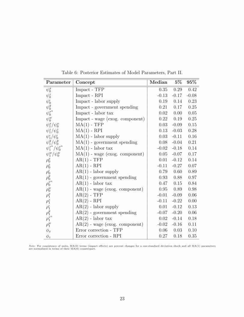
Table 6: Posterior Estimates of Model Parameters, Part II.
Parameter Concept Median 5% 95%
ψx0 Impact - TFP 0.35 0.29 0.42ψz0 Impact - RPI -0.13 -0.17 -0.08ψι0 Impact - labor supply 0.19 0.14 0.23ψg0 Impact - government spending 0.21 0.17 0.25ψτ
n
0 Impact - labor tax 0.02 0.00 0.05ψw0 Impact - wage (exog. component) 0.22 0.19 0.25ψx1/ψ
x0 MA(1) - TFP 0.03 -0.09 0.15
ψz1/ψz0 MA(1) - RPI 0.13 -0.03 0.28
ψι1/ψι0 MA(1) - labor supply 0.03 -0.11 0.16
ψg1/ψg0 MA(1) - government spending 0.08 -0.04 0.21
ψτn
1 /ψτn
0 MA(1) - labor tax -0.02 -0.18 0.14ψw1 /ψ
w0 MA(1) - wage (exog. component) 0.05 -0.07 0.17
ρx0 AR(1) - TFP 0.01 -0.12 0.14ρz0 AR(1) - RPI -0.11 -0.27 0.07ρι0 AR(1) - labor supply 0.79 0.60 0.89ρg0 AR(1) - government spending 0.93 0.88 0.97ρτ
n
0 AR(1) - labor tax 0.47 0.15 0.84ρw0 AR(1) - wage (exog. component) 0.95 0.89 0.98ρx1 AR(2) - TFP -0.01 -0.09 0.06ρz1 AR(2) - RPI -0.11 -0.22 0.00ρι1 AR(2) - labor supply 0.01 -0.12 0.13ρg1 AR(2) - government spending -0.07 -0.20 0.06ρτ
n
1 AR(2) - labor tax 0.02 -0.14 0.18ρw1 AR(2) - wage (exog. component) -0.02 -0.16 0.11φx Error correction - TFP 0.06 0.03 0.10φz Error correction - RPI 0.27 0.18 0.35
Note: For consistency of units, MA(0) terms (impact effects) are percent changes for a one-standard deviation shock and all MA(1) parametersare normalized in terms of their MA(0) counterpart.
23
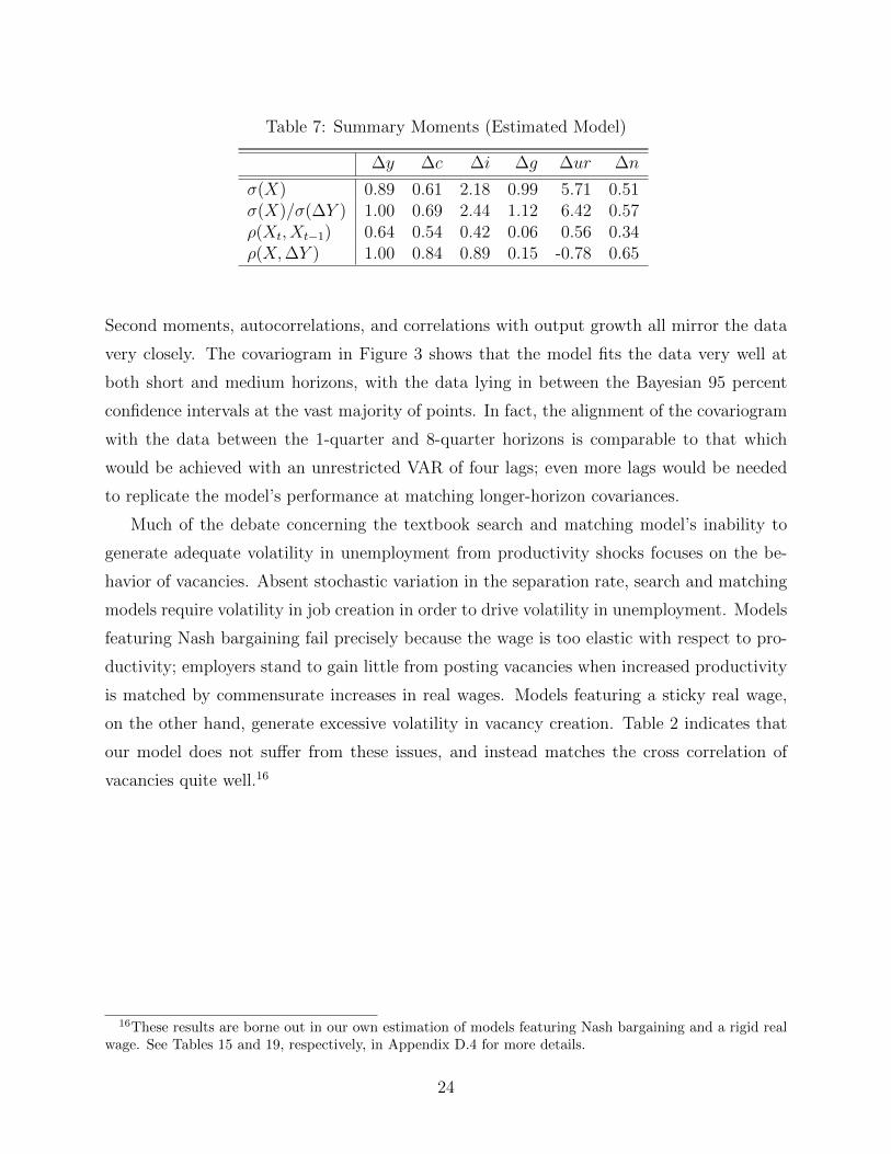
Table 7: Summary Moments (Estimated Model)
∆y ∆c ∆i ∆g ∆ur ∆n
σ(X) 0.89 0.61 2.18 0.99 5.71 0.51σ(X)/σ(∆Y ) 1.00 0.69 2.44 1.12 6.42 0.57ρ(Xt, Xt−1) 0.64 0.54 0.42 0.06 0.56 0.34ρ(X,∆Y ) 1.00 0.84 0.89 0.15 -0.78 0.65
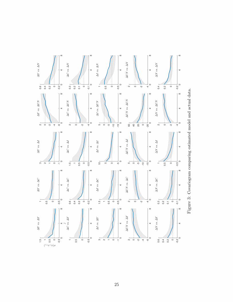
Second moments, autocorrelations, and correlations with output growth all mirror the data
very closely. The covariogram in Figure 3 shows that the model fits the data very well at
both short and medium horizons, with the data lying in between the Bayesian 95 percent
confidence intervals at the vast majority of points. In fact, the alignment of the covariogram
with the data between the 1-quarter and 8-quarter horizons is comparable to that which
would be achieved with an unrestricted VAR of four lags; even more lags would be needed
to replicate the model’s performance at matching longer-horizon covariances.
Much of the debate concerning the textbook search and matching model’s inability to
generate adequate volatility in unemployment from productivity shocks focuses on the be-
havior of vacancies. Absent stochastic variation in the separation rate, search and matching
models require volatility in job creation in order to drive volatility in unemployment. Models
featuring Nash bargaining fail precisely because the wage is too elastic with respect to pro-
ductivity; employers stand to gain little from posting vacancies when increased productivity
is matched by commensurate increases in real wages. Models featuring a sticky real wage,
on the other hand, generate excessive volatility in vacancy creation. Table 2 indicates that
our model does not suffer from these issues, and instead matches the cross correlation of
vacancies quite well.16
16These results are borne out in our own estimation of models featuring Nash bargaining and a rigid realwage. See Tables 15 and 19, respectively, in Appendix D.4 for more details.
24
04
8
j
-0.50
0.51
1.5
σ(xt,xt+j)
∆Y
vs.∆Y
04
8
-0.50
0.51
∆Y
vs.∆C
04
8
-1
0123∆Y
vs.∆I
04
8
-6-4-2
02∆Y
vs.∆UN
04
8
-0.20
0.2
0.4
0.6
∆Y
vs.∆N
04
8
-0.50
0.51
∆C
vs.∆Y
04
8
-0.20
0.2
0.4
0.6
∆C
vs.∆C
04
8
-0.50
0.51
1.5
∆C
vs.∆I
04
8
-4-2
02∆C
vs.∆UN
04
8
-0.10
0.1
0.2
0.3
∆C
vs.∆N
04
8
-1
0123∆Ivs.∆Y
04
8
-0.50
0.51
1.5
∆Ivs.∆C
04
8
-5
05
10
∆Ivs.∆I
04
8
-15
-10
-5
05∆Ivs.∆UN
04
8
-0.50
0.51
∆Ivs.∆N
04
8
-6-4-2
02∆UN
vs.∆Y
04
8
-4-2
02∆UN
vs.∆C
04
8
-15
-10
-5
05∆UN
vs.∆I
04
8
-200
20
40
60
∆UN
vs.∆UN
04
8
-4-2
02∆UN
vs.∆N
04
8
-0.20
0.2
0.4
0.6
∆N
vs.∆Y
04
8
-0.10
0.1
0.2
0.3
∆N
vs.∆C
04
8
-0.50
0.51
∆N
vs.∆I
04
8
-4-2
02∆N
vs.∆UN
04
8
-0.20
0.2
0.4
∆N
vs.∆N
Fig
ure
3:C
ovar
iogr
amco
mp
arin
ges
tim
ated
mod
elan
dac
tual
dat
a.
25

Table 3 compares the moments of the model-implied wage with the set of seven empirical
wage measures. The final row provides a summary measure of the precision of the information
contained in each wage series.17 These moments suggest that the compensation per worker
measure of the wage, as well as both ECI measures, are the most consistent with observed
quantities, given the model. The standard deviation, autocorrelation, and correlation with
output growth for compensation per worker are all quite close to the model-based wage. The
signal power in the final row suggests that both ECI measures also conform closely to the
model wage.
Figure 4 delves a bit deeper into the wage measurement relationships by comparing the
compensation per worker measure of cumulative wage growth with the model-implied wage
over the same period. Inspection of the figure confirms the results in Table 3: Compensation
per worker tracks the model-implied wage quite closely over the sample period. The figure
indicates that, while the series can differ in non-trivial ways over short horizons, the match
between the two series improves over longer time periods.
1972 1976 1980 1984 1988 1992 1996 2000 2004 2008 20122013
Year
-0.08
-0.06
-0.04
-0.02
0
0.02
0.04
0.06Measured
Smoothed
Figure 4: Compensation per worker and the smoothed model wage.
17We define the signal power of a particular wage measure i asV ar(γw,i∆ logwt)V ar(∆ log wi,t)
where wi,t denotes the
observation on empirical wage series i at time t.
26

4.2 Impulse Responses
Figure 5 documents impulse responses of the real wage and labor’s share of match surplus to
each of the six shocks in the model (five fundamental shocks plus the residual wage shock)
for three cases: our estimated model, Nash bargaining, and our rigid-wage model.18 By
construction, the wage in the rigid-wage model only responds to growth rate shocks and the
residual shock to wages. Furthermore, as expected, the share of match surplus accruing to
labor in the Nash bargaining model only responds to the residual shock to wages, as this may
be thought of as the wedge between the model wage and the structural Nash wage which
implies constant surplus shares.
The responses of the estimated wage process differ significantly from both the rigid-wage
model and the Nash bargaining model. The estimated wage responds to permanent shocks on
impact—more rapidly than the rigid-wage model—but is slightly muted relative to the Nash
bargaining wage response in the case of permanent technology shocks. Furthermore, the
estimated wage responds to investment-specific technology shocks and labor supply shocks
in a manner that is broadly consistent with the Nash bargaining responses, but deviates
from the Nash bargaining responses markedly for the government spending, labor tax, and
residual wage shocks. Indeed, there is no consistent similarity between the wage responses
in the estimated model, the rigid-wage model, and the Nash bargaining model. Moreover,
there is no evidence in our estimated process for wages that the data call for hump-shaped
responses of the real wage. Instead, in response to both permanent and temporary shocks, the
pattern is that of a substantial impact response of the wage followed by gradual adjustment
to its long-run level.
The impulse responses of labor’s share of match surplus demonstrate, in part, how the
estimated model achieves realistic volatility in labor market variables without requiring a
sticky real wage. Because of dynamic decision making on the part of firms and households,
the surplus shares depicted depend on the full path of future wages. Thus, despite the fact
that the two processes indicate very different impact effects for wages, both the rigid and
estimated wage processes result in a strong initial increase in the household’s share of surplus.
The estimated wage process is therefore simultaneously capturing both the impact effects of
real wages and the fluctuations in labor’s surplus share needed to deliver fluctuations in
18In computing impulse responses, we fix fundamental parameters at their values estimated in the baselineeconomy. Thus, differences in impulse responses in these figures are driven only by different assumptionsregarding wage determination.
27

5 10 15 20 25
0
0.2
0.4
0.6
0.8
1
1.2
5 10 15 20 25
-0.8
-0.6
-0.4
-0.2
0
5 10 15 20 25
0
0.05
0.1
0.15
0.2
5 10 15 20 25
-0.05
0
0.05
0.1
0.15
0.2
0.25
5 10 15 20 25
0
0.02
0.04
0.06
0.08
0.1
0.12
5 10 15 20 25
0
0.2
0.4
0.6
0.8
1
(a) Wage Level
5 10 15 20 25
-1
0
1
2
3
4
5
6
5 10 15 20 25
-2.5
-2
-1.5
-1
-0.5
0
0.5
1
5 10 15 20 25
-1
-0.5
0
0.5
1
1.5
2
5 10 15 20 25
-1
-0.5
0
0.5
1
1.5
5 10 15 20 25
-1
-0.5
0
0.5
5 10 15 20 25
-8
-6
-4
-2
0
2
(b) Surplus Share
Figure 5: Impulse responses to each of the six shocks.
28
5 10 15 20 25
0
0.5
1
1.5
2
5 10 15 20 25
0
0.2
0.4
0.6
0.8
1
1.2
5 10 15 20 25
0
0.5
1
1.5
2
2.5
3
3.5
5 10 15 20 25
0
0.2
0.4
0.6
0.8
1
1.2
5 10 15 20 25
-15
-10
-5
0
5
5 10 15 20 25
-5
0
5
10
15
Figure 6: Impulse responses to permanent neutral productivity shock.
vacancies and unemployment. This is possible because of the sluggish adjustment of wages
(relative to Nash bargaining) following the flexible initial response. Over time, the rigid-
wage model demonstrates a counterfactually large share of surplus accruing to firms, but
the qualitative response of the surplus share continues to resemble that of the rigid-wage
model. In short, while wages appear in many cases to roughly approximate the flexible Nash
benchmark, the implications for the division of surplus more closely resemble those of the
rigid-wage model.
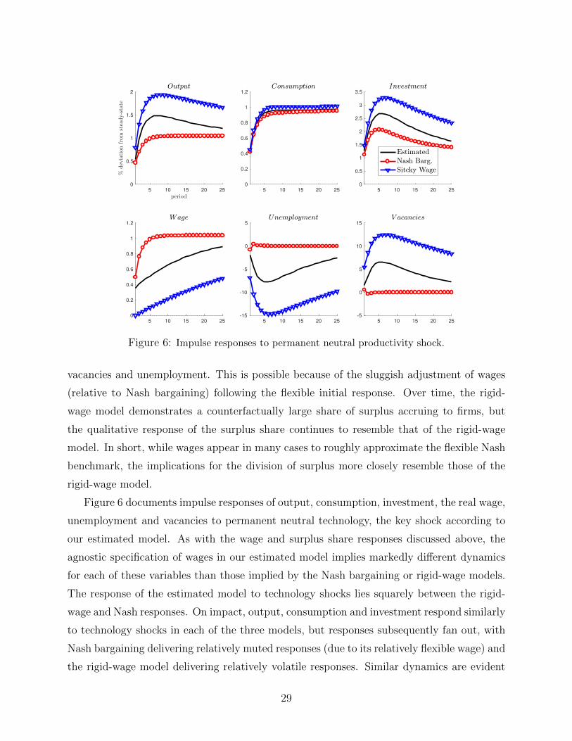
Figure 6 documents impulse responses of output, consumption, investment, the real wage,
unemployment and vacancies to permanent neutral technology, the key shock according to
our estimated model. As with the wage and surplus share responses discussed above, the
agnostic specification of wages in our estimated model implies markedly different dynamics
for each of these variables than those implied by the Nash bargaining or rigid-wage models.
The response of the estimated model to technology shocks lies squarely between the rigid-
wage and Nash responses. On impact, output, consumption and investment respond similarly
to technology shocks in each of the three models, but responses subsequently fan out, with
Nash bargaining delivering relatively muted responses (due to its relatively flexible wage) and
the rigid-wage model delivering relatively volatile responses. Similar dynamics are evident
29
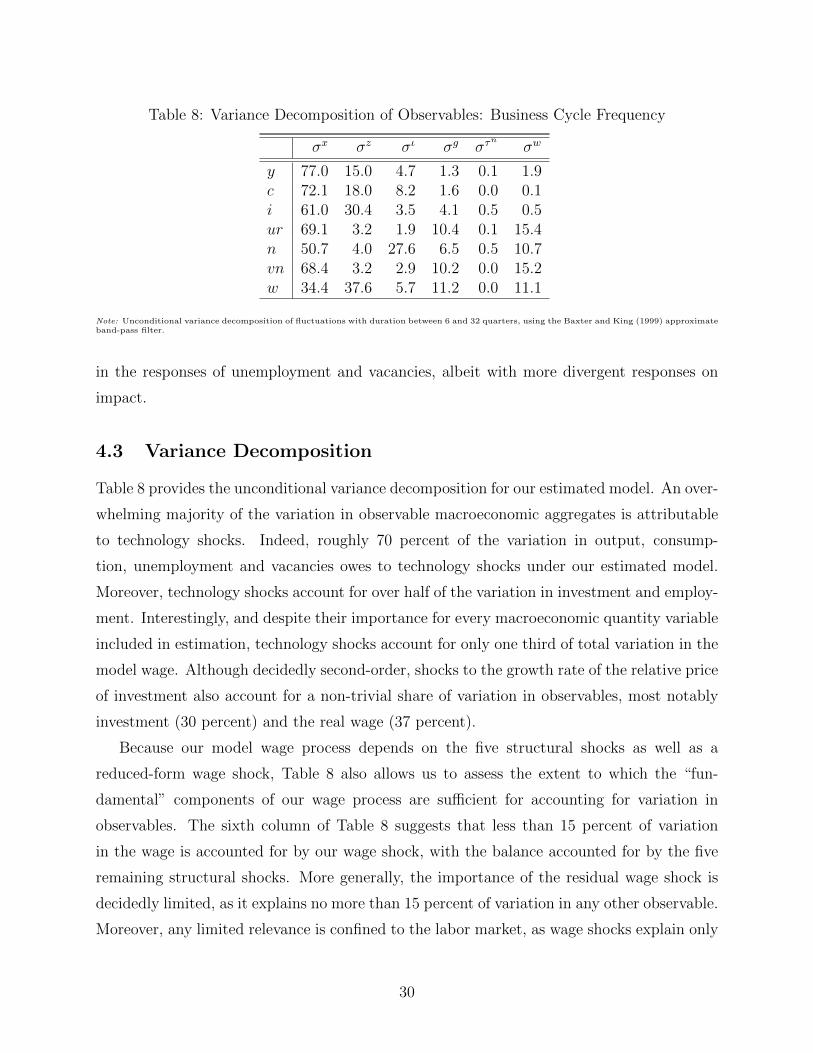
Table 8: Variance Decomposition of Observables: Business Cycle Frequency
σx σz σι σg στn
σw
y 77.0 15.0 4.7 1.3 0.1 1.9c 72.1 18.0 8.2 1.6 0.0 0.1i 61.0 30.4 3.5 4.1 0.5 0.5ur 69.1 3.2 1.9 10.4 0.1 15.4n 50.7 4.0 27.6 6.5 0.5 10.7vn 68.4 3.2 2.9 10.2 0.0 15.2w 34.4 37.6 5.7 11.2 0.0 11.1
Note: Unconditional variance decomposition of fluctuations with duration between 6 and 32 quarters, using the Baxter and King (1999) approximateband-pass filter.
in the responses of unemployment and vacancies, albeit with more divergent responses on
impact.
4.3 Variance Decomposition
Table 8 provides the unconditional variance decomposition for our estimated model. An over-
whelming majority of the variation in observable macroeconomic aggregates is attributable
to technology shocks. Indeed, roughly 70 percent of the variation in output, consump-
tion, unemployment and vacancies owes to technology shocks under our estimated model.
Moreover, technology shocks account for over half of the variation in investment and employ-
ment. Interestingly, and despite their importance for every macroeconomic quantity variable
included in estimation, technology shocks account for only one third of total variation in the
model wage. Although decidedly second-order, shocks to the growth rate of the relative price
of investment also account for a non-trivial share of variation in observables, most notably
investment (30 percent) and the real wage (37 percent).
Because our model wage process depends on the five structural shocks as well as a
reduced-form wage shock, Table 8 also allows us to assess the extent to which the “fun-
damental” components of our wage process are sufficient for accounting for variation in
observables. The sixth column of Table 8 suggests that less than 15 percent of variation
in the wage is accounted for by our wage shock, with the balance accounted for by the five
remaining structural shocks. More generally, the importance of the residual wage shock is
decidedly limited, as it explains no more than 15 percent of variation in any other observable.
Moreover, any limited relevance is confined to the labor market, as wage shocks explain only
30

Table 9: Model Comparison
Model P (M) Bayes Factor
Baseline 7471.5 exp(0)Nash Bargaining 7339.0 exp(132.5)Sticky Wage 7318.2 exp(153.3)
two percent of variation in output, and less than one percent of variation in consumption
and investment.
4.4 Model Comparison
We have suggested that our baseline model provides a substantial improvement in fit relative
to prominent structural models of wage determination. To make this comparison rigorous, we
estimate otherwise identical models with (i) a flexible Nash-bargained wage and (ii) a rigid
wage that adjusts only slowly in response to permanent shocks. For both of the alternative
models, we allow for exogenous ARMA(2,1) deviations from the underlying model of wage
determination, exactly analogous to the reduced-form wage shock in our baseline model. We
then perform a Bayesian model comparison, computing marginal likelihoods for the three
models we wish to consider. An important feature of this statistic is that it penalizes free
parameters, so that (nested) models with relatively more degrees of freedom are not always
preferred.19 Table 9 shows that, while the Nash bargaining model outperforms the sticky
real wage model, both are clearly dominated by our reduced-form specification for the wage,
with a Bayes factor on the order of exp(140).
The reasons for the failure of these two models are rather different, and in ways that
corroborate previous observations about these two wage-determination mechanisms. In par-
ticular, the model estimated with Nash bargaining is unable to generate sufficiently large
variation in vacancies, on account of an excessively volatile real wage. Interestingly, the data
do not seek a calibration that is consistent with Hagedorn and Manovskii’s (2008) sugges-
tion of a low bargaining power combined with a high replacement rate of benefits (median
estimates are η = 0.41 and κ = 0.46, respectively). Conversely, the tables in Appendix D.4
show that the rigid-wage economy delivers counterfactually high volatility of unemployment
19Since our estimation relies very little any of the MA(1) or AR(2) terms we have included in the baselinemodel of the wage, our comparison actually implicitly penalizes it.
31

and, to a lesser extent, output growth.
4.5 Discussion
We believe our results deliver several important insights that can guide future researchers
considering alternative models of wage determination. First, our results — in particular
the comparison to the alternative models — provide strong evidence that the endogenous
response of wages to fundamental shocks is crucial for our model to match the data. If causal-
ity in the economy was passing from exogenous shocks in wage determination to the broader
economy, then the alternative models could easily account for such fluctuations through the
exogenous component of the wage process. Instead, the large role of fundamental shocks (and
relatively small role of exogenous wage shocks) in the baseline economy supports the conclu-
sion that wages are an endogenous outcome. The orthogonal wage shocks in our model may
then be thought of as deviations from an underlying wage-determination paradigm through
which fundamental shocks drive wages. Unable to account for the endogenous pattern of
wage fluctuations, the alternative models rely far more heavily on the exogenous component
of wages to best-fit the data, and do so without approaching the fit provided by the baseline
model.
Second, we have shown that the data are consistent with relatively flexible real wages
and demand an important role for productivity shocks in driving both real quantities and
labor market variables. In Appendix D.4, we provide variance decompositions for the esti-
mated models featuring Nash bargaining and a rigid real wage, respectively. Interestingly,
the data do not demand a dominant role for productivity shocks in either case. In the case of
Nash bargaining, productivity shocks account for non-labor market variables—output, con-
sumption, and investment—but fail to account for any significant variation in labor market
quantities. This is consistent with the critique of Shimer (2005). Perhaps more surprisingly,
in the case of the rigid wage model, productivity shocks play a substantial but smaller role
than in the baseline economy. By construction, productivity shocks can account for very
little of the variation in the real wage, leading the model to depend largely on residual wage
shocks to explain wage fluctuations, and thus to a strongly counterfactual countercyclical
real wage.
By contrast, when the model is estimated with our more general wage specification,
the data demand a central role for productivity shocks. Our wage specification allows for
this precisely because it can accommodate wage fluctuations that are significantly correlated
32
1972 1976 1980 1984 1988 1992 1996 2000 2004 2008 20122013
Year
0.9
0.91
0.92
0.93
0.94
0.95
0.96
0.97
Smoothed Labor Surplus Share
Figure 7: Labor’s share of surplus.
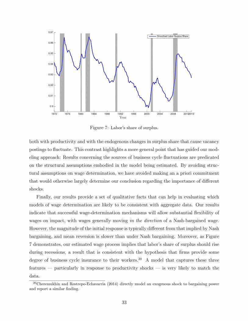
both with productivity and with the endogenous changes in surplus share that cause vacancy
postings to fluctuate. This contrast highlights a more general point that has guided our mod-
eling approach: Results concerning the sources of business cycle fluctuations are predicated
on the structural assumptions embodied in the model being estimated. By avoiding struc-
tural assumptions on wage determination, we have avoided making an a priori commitment
that would otherwise largely determine our conclusion regarding the importance of different
shocks.
Finally, our results provide a set of qualitative facts that can help in evaluating which
models of wage determination are likely to be consistent with aggregate data. Our results
indicate that successful wage-determination mechanisms will allow substantial flexibility of
wages on impact, with wages generally moving in the direction of a Nash-bargained wage.
However, the magnitude of the initial response is typically different from that implied by Nash
bargaining, and mean reversion is slower than under Nash bargaining. Moreover, as Figure
7 demonstrates, our estimated wage process implies that labor’s share of surplus should rise
during recessions, a result that is consistent with the hypothesis that firms provide some
degree of business cycle insurance to their workers.20 A model that captures these three
features — particularly in response to productivity shocks — is very likely to match the
data.
20Cheremukhin and Restrepo-Echavarria (2014) directly model an exogenous shock to bargaining powerand report a similar finding.
33

5 Conclusion
The search and matching framework has become a popular modeling device in mainstream
macroeconomics. But no consensus has been reached on the nature of wage determination in
such markets. We draw upon search theory for what we consider to be critical components
for realistically representing market interactions–costly search, nontrivial job-finding rates,
equilibrium unemployment–while dispensing with a priori wage-determination mechanisms.
Instead, we model wages as evolving according to an ARMA process, thus approximately
nesting most structural wage-determination mechanisms used in the literature. We can do
this because the search and matching framework per se requires nothing of wages except that
they remain within the bargaining set. The flexibility of our approach allows us to study
the empirical properties of the search and matching framework constraining ourselves to a
particular theory of wages. The wage process that we estimate sheds light on the properties
that a data-consistent theory of the wage must have.
Our model is able to match the data remarkably well. We match key business cycle
frequency moments of output, consumption, investment, employment and the unemployment
rate with a high level of accuracy relative to existing DSGE estimation literature. The
dynamics of our estimated model are driven primarily by permanent shocks to productivity
while our estimated process for the wage suggests that real wages can be relatively flexible,
while still generating empirically realistic cyclical fluctuations. This result stands in marked
contrast with a large literature seeking amplification by way of nominal rigidities or other
partial adjustment mechanisms.
References
Altug, S. (1989). Time-to-build and aggregate fluctuations: Some new evidence. Interna-
tional Economic Review 30 (4), pp. 889–920.
Andolfatto, D. (1996, March). Business cycles and labor-market search. American Economic
Review 86 (1), 112–32.
Arseneau, D. M. and S. K. Chugh (2012). Tax Smoothing in Frictional Labor Markets.
Journal of Political Economy 120 (5), 926–985.
34

Baxter, M. and R. G. King (1999). Measuring Business Cycles: Approximate Band-Pass
Filters For Economic Time Series. The Review of Economics and Statistics 81 (4), 575–593.
Boivin, J. and M. Giannoni (2006, December). DSGE Models in a Data-Rich Environment.
Working Paper 12772, National Bureau of Economic Research.
Chari, V. V., P. J. Kehoe, and E. R. McGrattan (2007). Business cylce accounting. Econo-
metrica 75 (3), pp. 781–836.
Cheremukhin, A. A. and P. Restrepo-Echavarria (2014). The labor wedge as a matching
friction. European Economic Review 68 (0), 71 – 92.
Christiano, L. J., M. Eichenbaum, and C. L. Evans (2005). Nominal Rigidities and the
Dynamic Effects of a Shock to Monetary Policy. Journal of Political Economy 113 (1),
1–45.
Christiano, L. J., M. S. Eichenbaum, and M. Trabandt (2016). Unemployment and business
cycles. Econometrica 84 (4), 1523–1569.
Davis, S. J., R. J. Faberman, and J. Haltiwanger (2006, April). The flow approach to labor
markets: New data sources and micro-macro links. Working Paper 12167, National Bureau
of Economic Research.
Diamond, P. A. (1982). Aggregate demand management in search equilibrium. Journal of
Political Economy 90 (5), pp. 881–894.
Farmer, R. E. A. and A. Hollenhorst (2006, October). Shooting the Auctioneer. NBER
Working Papers 12584, National Bureau of Economic Research, Inc.
Gertler, M., L. Sala, and A. Trigari (2008). An estimated monetary dsge model with unem-
ployment and staggered nominal wage bargaining. Journal of Money, Credit and Bank-
ing 40 (8), 1713–1764.
Haefke, C., M. Sonntag, and T. van Rens (2013a). Wage rigidity and job creation. Journal
of Monetary Economics 60 (8), 887 – 899.
Haefke, C., M. Sonntag, and T. van Rens (2013b). Wage rigidity and job creation. Journal
of Monetary Economics 60 (8), 887 – 899.
35

Hagedorn, M. and I. Manovskii (2008, September). The Cyclical Behavior of Equilibrium
Unemployment and Vacancies Revisited. American Economic Review 98 (4), 1692–1706.
Hall, G. J. (1996). Overtime, effort, and the propagation of business cycle shocks. Journal
of Monetary Economics 38 (1), 139 – 160.
Hall, R. E. (2005). Employment fluctuations with equilibrium wage stickiness. The American
Economic Review 95 (1), 50–65.
Hall, R. E. and P. R. Milgrom (2008, September). The Limited Influence of Unemployment
on the Wage Bargain. American Economic Review 98 (4), 1653–74.
Ireland, P. N. (2004). A Method For Taking Models to the Data. Journal of Economic
Dynamics and Control 28 (6), 1205 – 1226.
Iskrev, N. (2010). Local Identification in DSGE Models. Journal of Monetary Eco-
nomics 57 (2), 189 – 202.
Kennan, J. (2010). Private Information, Wage Bargaining and Employment Fluctuations.
Review of Economic Studies 77 (2), 633–664.
Kudlyak, M. (2014). The cyclicality of the user cost of labor. Journal of Monetary Eco-
nomics (0), –.
Lubik, T. (2009). Estimating a search and matching model of the aggregate labor market.
FRB Richmond Economic Quarterly 95 (2), 101–120.
McGrattan, E. R. (1994, June). The macroeconomic effects of distortionary taxation. Journal
of Monetary Economics 33 (3), 573–601.
Merz, M. (1995, November). Search in the labor market and the real business cycle. Journal
of Monetary Economics 36 (2), 269–300.
Meyer-Gohde, A. and D. Neuhoff (2014). Generalized exogenous processes in dsge: A
bayesian approach. Technical report, Humboldt University.
Michaillat, P. (2012). Do matching frictions explain unemployment? not in bad times.
American Economic Review 102 (4).
36
Michaillat, P. and E. Saez (2013, February). A model of aggregate demand and unemploy-
ment. Working Paper 18826, National Bureau of Economic Research.
Mortensen, D. T. (1982). Property rights and efficiency in mating, racing, and related games.
The American Economic Review 72 (5), pp. 968–979.
Mortensen, D. T. (1992). Search theory and macroeconomics: A review essay. Journal of
Monetary Economics 29 (1), 163 – 167.
Mortensen, D. T. and C. A. Pissarides (1994, July). Job Creation and Job Destruction in
the Theory of Unemployment. Review of Economic Studies 61 (3), 397–415.
Pissarides, C. A. (1985). Short-run equilibrium dynamics of unemployment, vacancies, and
real wages. The American Economic Review 75 (4), pp. 676–690.
Pissarides, C. A. (2009). The unemployment volatility puzzle: Is wage stickiness the answer?
Econometrica 77 (5), 1339–1369.
Rogerson, R. and R. Shimer (2011). Chapter 7 - search in macroeconomic models of the
labor market. Volume 4, Part A of Handbook of Labor Economics, pp. 619 – 700. Elsevier.
Sargent, T. J. (1989, April). Two models of measurements and the investment accelerator.
Journal of Political Economy 97 (2), 251–87.
Schmitt-Grohe, S. and M. Uribe (2012). What’s News in Business Cycles. Econometrica 80,
2733–2764.
Shimer, R. (2005). The cyclical behavior of equilibrium unemployment and vacancies. The
American Economic Review 95 (1), pp. 25–49.
Smets, F. and R. Wouters (2007, June). Shocks and Frictions in US Busines Cycle: a
Bayesian DSGE Approach. American Economic Review 97 (3), 586–606.
Solon, G., R. Barsky, and J. A. Parker (1994). Measuring the cyclicality of real wages: How
important is composition bias. The Quarterly Journal of Economics 109 (1), pp. 1–25.
37
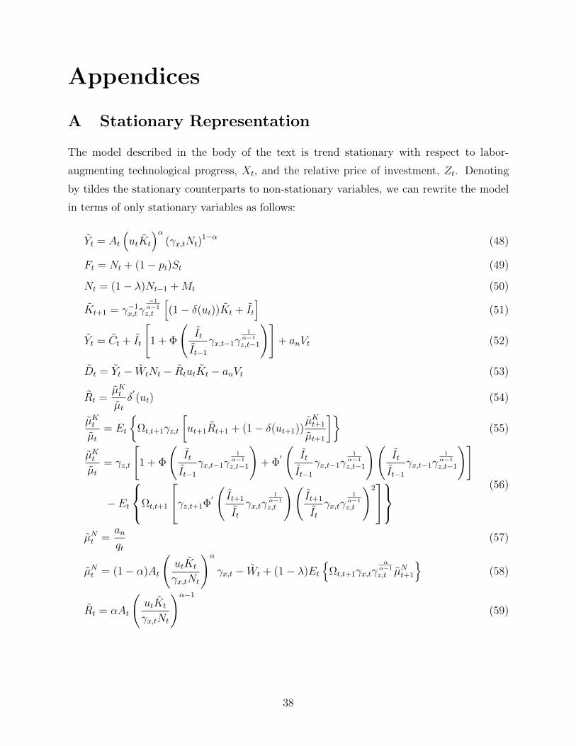
Appendices
A Stationary Representation
The model described in the body of the text is trend stationary with respect to labor-
augmenting technological progress, Xt, and the relative price of investment, Zt. Denoting
by tildes the stationary counterparts to non-stationary variables, we can rewrite the model
in terms of only stationary variables as follows:
Yt = At
(utKt
)α(γx,tNt)
1−α (48)
Ft = Nt + (1− pt)St (49)
Nt = (1− λ)Nt−1 +Mt (50)
Kt+1 = γ−1x,tγ
−1α−1
z,t
[(1− δ(ut))Kt + It
](51)
Yt = Ct + It
[1 + Φ
(It
It−1
γx,t−1γ1
α−1
z,t−1
)]+ anVt (52)
Dt = Yt − WtNt − RtutKt − anVt (53)
Rt =µKtµtδ′(ut) (54)
µKtµt
= Et
Ωt,t+1γz,t
[ut+1Rt+1 + (1− δ(ut+1))
µKt+1
µt+1
](55)
µKtµt
= γz,t
[1 + Φ
(It
It−1
γx,t−1γ1
α−1
z,t−1
)+ Φ
′
(It
It−1
γx,t−1γ1
α−1
z,t−1
)(It
It−1
γx,t−1γ1
α−1
z,t−1
)]
− Et
Ωt,t+1
γz,t+1Φ′
(It+1
Itγx,tγ
1α−1
z,t
)(It+1
Itγx,tγ
1α−1
z,t
)2
(56)
µNt =anqt
(57)
µNt = (1− α)At
(utKt
γx,tNt
)α
γx,t − Wt + (1− λ)Et
Ωt,t+1γx,tγ
αα−1
z,t µNt+1
(58)
Rt = αAt
(utKt
γx,tNt
)α−1
(59)
38

− uf,tuc,t
= pt
[Wt + (1− λ)Et
Ωt,t+1(γx,tγ
αα−1
z,t )1−σ(
1− pt+1
pt+1
)(−uf,t+1
uc,t+1
− κt+1
)]+ (1− pt)κt
(60)
where
Ωt,t+1 ≡ βµt+1
µt
(γx,tγ
αα−1
z,t
)−σ(61)
µt =µt(
Xt−1Zαα−1
t−1
)−σ (62)
µKt =µKt(
Xt−1Zαα−1
t−1
)−σZt−1
(63)
µNt =µNt
Xt−1Zαα−1
t−1
(64)
and variables are detrended according to ∆t ≡ ∆t
Xt−1Zαα−1t−1
for ∆t ∈ Yt, Ct, Dt,Wt, ∆t ≡∆t
Xt−1Z1
α−1t−1
for ∆t ∈ Kt, It, and Rt ≡ RtZt
.
B Steady State and Calibration
We use the restrictions imposed by the deterministic steady-state of the model, together
with long-run values for p, q, N , un, φN , u taken from the data, to analytically solve for
values for all remaining endogenous variables, as well as χ, λ, ψ, an, δ1 and W . In what
follows, we make reference only to detrended variables, though we neglect tildes for ease of
notation.
The first-order conditions for investment and utilization, evaluated at the deterministic
steady state, imply
µK/µ = γz (65)
R = (µK/µ)δ1. (66)
Substituting these expressions into the household’s first-order condition for period-ahead
capital and solving for δ1, we obtain
δ1 =[(Ωγz)
−1 − 1 + δ0
]/u (67)
39

from which we recover
R = γzδ1. (68)
From the firm’s first-order condition for capital, we obtain
K =[αAuα−1(γxN)1−αr−1
] 11−α (69)
from which, in turn, we can solve for output
Y = A(uK)α(γxN)1−α. (70)
The definition of the unemployment rate, together with its long-run value and that of total
employment, can be used to solve for steady-state labor force participation
F =N
1− un. (71)
The definition of the labor force, in turn, allows us to solve for the mass of searching workers,
S =F − N1− p
. (72)
The law of motion for employment (from the perspective of the household and the firm,
respectively) yield
λ =pS
N(73)
V =λN
q. (74)
From the definition of the matching function, we obtain
θ =p
q(75)
which in turn allows us to solve for χ,
χ = pθ−ε. (76)
Next, from the definition of labor’s share, together with its steady state value φN , we can
40

solve for the real wage,
W = φNN−αA(uK)αγ1−αx . (77)
With the steady-state real wage in hand, we use the vacancy posting condition to solve for
the vacancy posting cost
an =q
1− (1− λ)Ωγxγαα−1z
[(1− α)A
(uK
Nγx
)α−W
](78)
where Ω = β(γxγ
αα−1z
)−σ. The law of motion for capital and the aggregate resource con-
straint imply, respectively,
I = K
1− (1− δ0)γ−1x γ
−1α−1z
γ−1x γ
−1α−1z
(79)
and
C = Y −G− anV − γzI. (80)
Finally, making use of the labor force participation condition, we obtain
ψ =
W
[p+ (1− p)κ− κ(1− λ)β (1− p)
(γxγ
αα−1z
)1−σ]
(1− (1− λ)β (1− p)
(γxγ
αα−1z
)1−σ)(
(1− F )−ιC(1− h(γxγαα−1z )−1)
) . (81)
C Match Surplus and Nash Bargaining
In order to compare the dynamics of our estimated model with those implied by Nash
bargaining, we first use the expressions for household and firm match surpluses to derive
the wage associated with Nash bargaining in our model. This also yields expressions for
household and firm match surplus shares, which we discuss in the body of the text.
The wage that results from Nash bargaining between firms and workers is given by
WNBt = arg max
Wt
[Wt(Wt)−Ut]η[Jt(Wt)−Vt]
1−η (82)
where Wt denotes the value of a match for the household, Ut denotes the value of unem-
ployment for the household, Jt denotes the value of a match for the firm, and Vt denotes the
41

value of a vacancy for the firm. Free-entry of firms implies that Vt = 0, and our specification
of unemployment benefits, combined with the existence of a search margin for households,
implies that Ut = κt. Thus, the standard Nash sharing rule reduces to
Wt −Ut =
(η
1− η
)Jt. (83)
The household match surplus (in units of consumption) may be expressed as the sum of the
wage payment earned in the period of the match (due to our timing assumption) and the
continuation value of the match, less the lump-sum transfer to the unemployed,
Wt −Ut = Wt(1− τnt )− κt + (1− λ)Et (1− pt+1)Ωt,t+1(Wt+1 −Ut+1) . (84)
The value of a match to the firm (again, in units of consumption) is given by the current
marginal product of the match net of the wage bill plus the continuation value,
Jt = AtFn,t −Wt + (1− λ)Et Ωt,t+1Jt+1 . (85)
Note that the firm’s first-order conditions imply
Jt = µNt . (86)
To solve for the wage associated with Nash bargaining, begin by substituting the expressions
for Wt and Ut into the Nash sharing rule,
WNBt (1− τnt )− κt + (1− λ)Et (1− pt+1)Ωt,t+1(Wt+1 −Ut+1) =
η
1− ηJt. (87)
Iterating the sharing rule forward and substituting in for Wt+1 −Ut+1,
WNBt (1− τnt )− κt + (1− λ)Et
(1− pt+1)Ωt,t+1
(η
1− η
)Jt+1
=
η
1− ηJt. (88)
Replacing Jt with the firm’s first-order condition for labor and then Jt+1 with the time t+ 1
42
Lagrange multiplier,
WNBt (1− τnt )− κt + (1− λ)Et
(1− pt+1)Ωt,t+1
(η
1− η
)µNt+1
=
η
1− η(AtFn,t −WNB
t + (1− λ)Et
Ωt,t+1µNt+1
).
(89)
Solving for WNBt , we obtain
WNBt =
1− ηη + (1− η)(1− τnt )
κt +η
η + (1− η)(1− τnt )
[AtFn,t + (1− λ)Et
Ωt,t+1pt+1µ
Nt+1
].
(90)
From here, dividing by Xt−1Zαα−1
t−1 yields the stationary representation,
WNBt =
1− ηη + (1− η)(1− τnt )
κt+η
η + (1− η)(1− τnt )
[AtFn,t + (1− λ)γx,tγ
αα−1
z,t Et
Ωt,t+1pt+1µNt+1
].
(91)
Then, for a given wage-determination mechanism, the standard expression for the house-
hold’s share of match surplus is given by
SSH =W −U
W −U + J−V(92)
and the expression for the firm’s share of match surplus is
SSF =J−V
W −U + J−V= 1− SSH . (93)
D Estimation Details
D.1 Data Construction
Nominal quantity variables are converted to their real per capita counterparts by dividing
by the seasonally-adjusted chain-weighted GDP deflator and the civilian non-institutional
population. Consumption is measured as the sum of personal consumption expenditures on
non-durables and services, while investment is measured as the sum of personal consumption
expenditure on durables and total private fixed investment. Unemployment is measured as
the number of unemployed persons as a percentage of the civilian non-institutional labor
force. The labor tax series is constructed by Arseneau and Chugh (2012), and ends in
2009Q4.
43
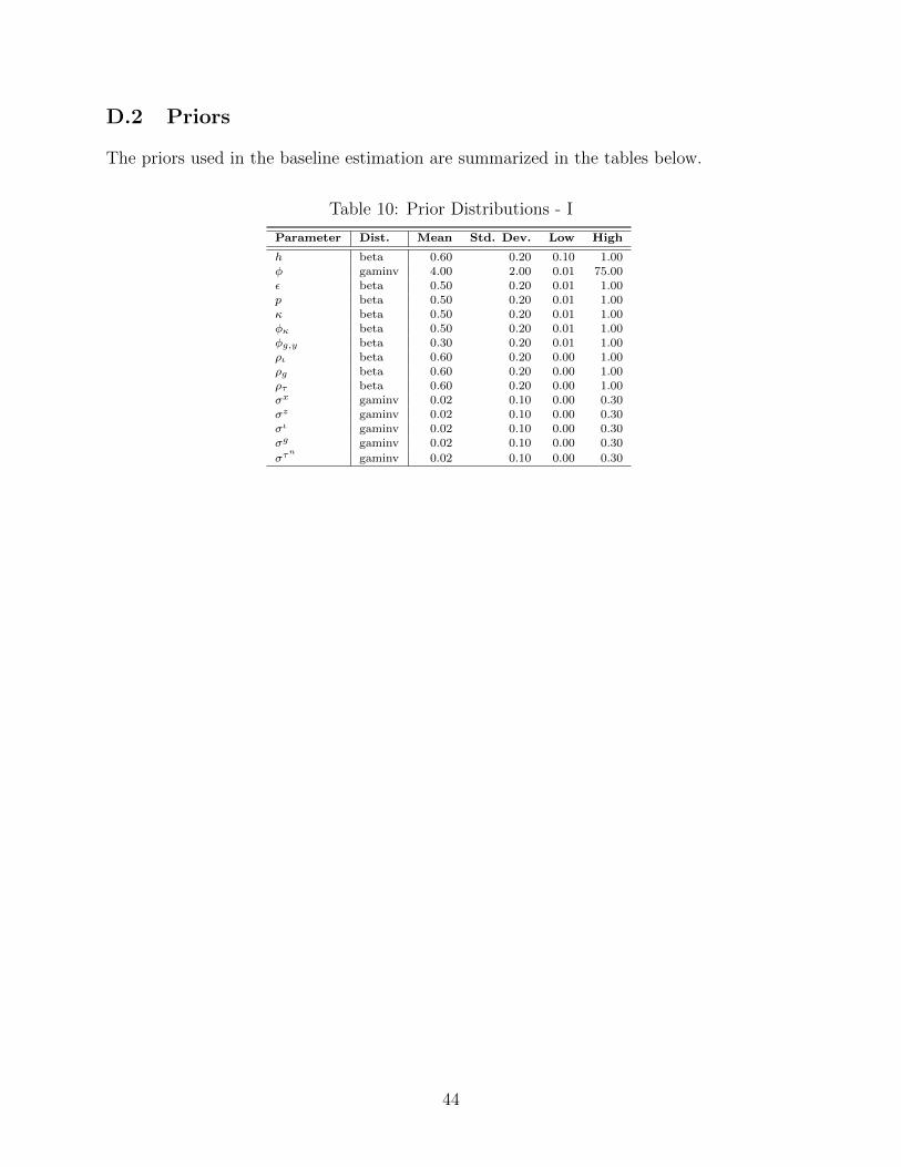
D.2 Priors
The priors used in the baseline estimation are summarized in the tables below.
Table 10: Prior Distributions - I
Parameter Dist. Mean Std. Dev. Low High
h beta 0.60 0.20 0.10 1.00φ gaminv 4.00 2.00 0.01 75.00ε beta 0.50 0.20 0.01 1.00p beta 0.50 0.20 0.01 1.00κ beta 0.50 0.20 0.01 1.00φκ beta 0.50 0.20 0.01 1.00φg,y beta 0.30 0.20 0.01 1.00ρι beta 0.60 0.20 0.00 1.00ρg beta 0.60 0.20 0.00 1.00ρτ beta 0.60 0.20 0.00 1.00σx gaminv 0.02 0.10 0.00 0.30σz gaminv 0.02 0.10 0.00 0.30σι gaminv 0.02 0.10 0.00 0.30σg gaminv 0.02 0.10 0.00 0.30
στn
gaminv 0.02 0.10 0.00 0.30
44

Table 11: Prior Distributions - II
Parameter Dist. Mean Std. Dev. Low High
ψx0 gaminv 1.00 1.00 0.00 5.00ψz0 norm 0.00 1.00 -5.00 5.00ψι0 norm 0.00 1.00 -5.00 5.00ψg0 norm 0.00 1.00 -5.00 5.00
ψτn
0 norm 0.00 1.00 -5.00 5.00ψw0 gaminv 1.00 1.00 0.00 5.00ψx1 /ψ
x0 norm 0.00 0.10 -0.99 0.99
ψz1/ψz0 norm 0.00 0.10 -0.99 0.99
ψι1/ψι0 norm 0.00 0.10 -0.99 0.99
ψg1/ψg0 norm 0.00 0.10 -0.99 0.99
ψτn
1 /ψτn
0 norm 0.00 0.10 -0.99 0.99ψw1 /ψ
w0 norm 0.00 0.10 -0.99 0.99
ρx0 norm 0.00 0.10 -0.99 0.99ρz0 norm 0.00 0.10 -0.99 0.99ρι0 beta 0.50 0.20 0.00 1.00ρg0 beta 0.50 0.20 0.00 1.00
ρτn
0 beta 0.50 0.20 0.00 1.00ρw0 beta 0.50 0.20 0.00 1.00ρx1 norm 0.00 0.10 -0.99 0.99ρz1 norm 0.00 0.10 -0.99 0.99ρι1 norm 0.00 0.10 -0.99 0.99ρg1 norm 0.00 0.10 -0.99 0.99
ρτn
1 norm 0.00 0.10 -0.99 0.99ρw1 norm 0.00 0.10 -0.99 0.99φx beta 0.50 0.20 0.00 1.00φz beta 0.50 0.20 0.00 1.00
Table 12: Prior Distributions - III
Parameter Dist. Mean Std. Dev. Low High
γw,1 gaminv 1.00 0.20 0.00 5.00γw,2 gaminv 1.00 0.20 0.00 5.00γw,3 gaminv 1.00 0.20 0.00 5.00γw,4 gaminv 1.00 0.20 0.00 5.00γw,5 gaminv 1.00 0.20 0.00 5.00γw,6 gaminv 1.00 0.20 0.00 5.00γw,7 gaminv 1.00 0.20 0.00 5.00γv,1 gaminv 1.00 0.20 0.00 5.00γv,2 gaminv 1.00 0.20 0.00 5.00σy gaminv 0.00 0.03 0.00 0.20σw,1 gaminv 0.00 0.03 0.00 0.20σw,2 gaminv 0.00 0.03 0.00 0.20σw,3 gaminv 0.00 0.03 0.00 0.20σw,4 gaminv 0.00 0.03 0.00 0.20σw,5 gaminv 0.00 0.03 0.00 0.20σw,6 gaminv 0.00 0.03 0.00 0.20σw,7 gaminv 0.00 0.03 0.00 0.20σv,1 gaminv 0.01 0.03 0.00 2.00σv,2 gaminv 0.01 0.03 0.00 2.00
45

D.3 Estimated Model
We compute the posterior parameter distribution using the MCMC algorithm with 12 chains
of 1.5 million draws each and dropping the first 25% of each chain. This appendix summarizes
the estimated parameters for the measurement equations (45)-(46), and provides impulses re-
sponses for the main quantities and labor market variables for each of the model’s six shocks.
The final figure also plots prior and posterior distributions for the estimated parameters.
Table 13: Posterior Estimates of Model Parameters, Part III.
Parameter Concept Median 5% 95%
γw,1 Wage loading - Total comp. per worker 0.62 0.53 0.73γw,2 Wage loading - Comp. per hour index 0.60 0.50 0.72γw,3 Wage loading - Real weekly comp. 0.74 0.60 0.93γw,4 Wage loading - ECI (wages) 0.41 0.35 0.46γw,5 Wage loading - ECI (wages and benefits) 0.42 0.37 0.49γw,6 Wage loading - Quality-adj. wage (HSvR) 0.73 0.58 0.92γw,7 Wage loading - Quality-adj. wage for new workers (HSvR) 0.93 0.70 1.28γv,1 Vacancy loading - JOLTS survey 1.01 0.82 1.25γv,2 Vacancy loading - Help-wanted 2.23 1.89 2.65σy Meas. error - GDP 0.00 0.00 0.01σw,1 Measurement error - Total comp. per worker 0.01 0.01 0.01σw,2 Measurement error - Comp. per hour index 0.01 0.01 0.01σw,3 Measurement error - Real weekly comp. 0.01 0.01 0.01σw,4 Measurement error - ECI (wages) 0.00 0.00 0.00σw,5 Measurement error - ECI (wages and benefits) 0.00 0.00 0.00σw,6 Measurement error - Quality-adj. wage (HSvR) 0.01 0.01 0.01σw,7 Measurement error - Quality-adj. wage for new workers (HSvR) 0.05 0.05 0.06σv,1 Measurement error - JOLTS survey 0.04 0.04 0.05σv,2 Measurement error - Help-wanted 0.03 0.03 0.04
46
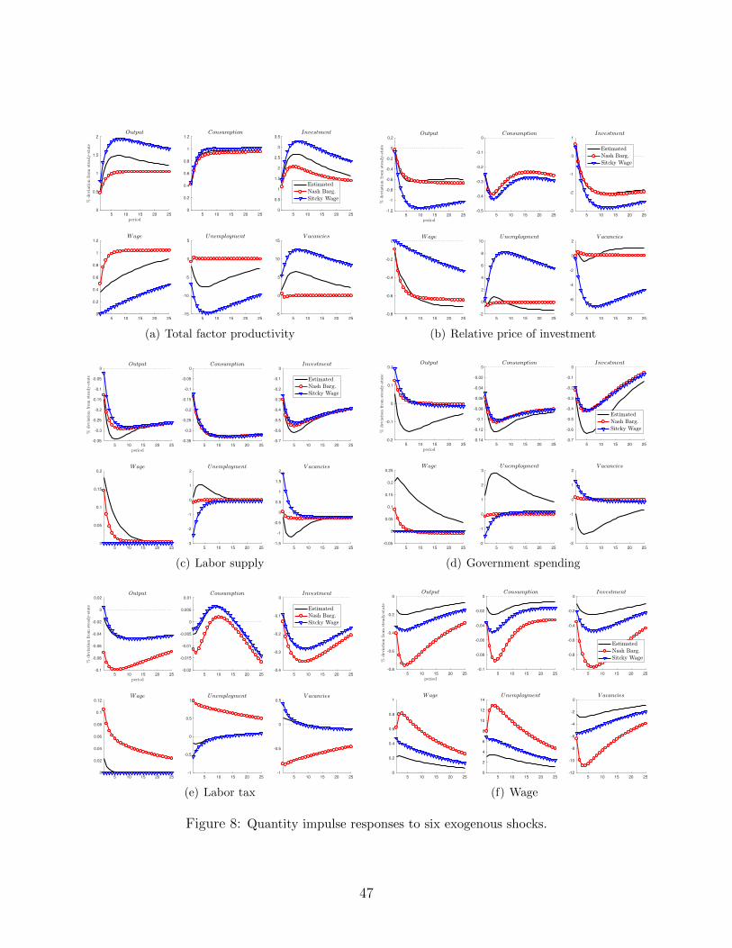
5 10 15 20 25
0
0.5
1
1.5
2
5 10 15 20 25
0
0.2
0.4
0.6
0.8
1
1.2
5 10 15 20 25
0
0.5
1
1.5
2
2.5
3
3.5
5 10 15 20 25
0
0.2
0.4
0.6
0.8
1
1.2
5 10 15 20 25
-15
-10
-5
0
5
5 10 15 20 25
-5
0
5
10
15
(a) Total factor productivity
5 10 15 20 25
-1.2
-1
-0.8
-0.6
-0.4
-0.2
0
0.2
5 10 15 20 25
-0.5
-0.4
-0.3
-0.2
-0.1
0
5 10 15 20 25
-3
-2
-1
0
1
5 10 15 20 25
-0.8
-0.6
-0.4
-0.2
0
5 10 15 20 25
-2
0
2
4
6
8
10
5 10 15 20 25
-8
-6
-4
-2
0
2
(b) Relative price of investment
5 10 15 20 25
-0.35
-0.3
-0.25
-0.2
-0.15
-0.1
-0.05
0
5 10 15 20 25
-0.35
-0.3
-0.25
-0.2
-0.15
-0.1
-0.05
0
5 10 15 20 25
-0.7
-0.6
-0.5
-0.4
-0.3
-0.2
-0.1
0
5 10 15 20 25
0
0.05
0.1
0.15
0.2
5 10 15 20 25
-3
-2
-1
0
1
2
5 10 15 20 25
-1.5
-1
-0.5
0
0.5
1
1.5
2
(c) Labor supply
5 10 15 20 25
-0.2
-0.1
0
0.1
0.2
5 10 15 20 25
-0.14
-0.12
-0.1
-0.08
-0.06
-0.04
-0.02
0
5 10 15 20 25
-0.7
-0.6
-0.5
-0.4
-0.3
-0.2
-0.1
0
5 10 15 20 25
-0.05
0
0.05
0.1
0.15
0.2
0.25
5 10 15 20 25
-2
-1
0
1
2
3
5 10 15 20 25
-3
-2
-1
0
1
2
(d) Government spending
5 10 15 20 25
-0.1
-0.08
-0.06
-0.04
-0.02
0
0.02
5 10 15 20 25
-0.02
-0.015
-0.01
-0.005
0
0.005
0.01
5 10 15 20 25
-0.4
-0.3
-0.2
-0.1
0
5 10 15 20 25
0
0.02
0.04
0.06
0.08
0.1
0.12
5 10 15 20 25
-1
-0.5
0
0.5
1
5 10 15 20 25
-1
-0.5
0
0.5
(e) Labor tax
5 10 15 20 25
-0.8
-0.6
-0.4
-0.2
0
5 10 15 20 25
-0.1
-0.08
-0.06
-0.04
-0.02
0
5 10 15 20 25
-1
-0.8
-0.6
-0.4
-0.2
0
5 10 15 20 25
0
0.2
0.4
0.6
0.8
1
5 10 15 20 25
0
2
4
6
8
10
12
14
5 10 15 20 25
-12
-10
-8
-6
-4
-2
0
(f) Wage
Figure 8: Quantity impulse responses to six exogenous shocks.
47

0.20.40.60.8 1
h
0 20 40 60
φ
0.20.40.60.8 1
ε
0.20.40.60.8 1
p
0.20.40.60.8 1
κ
0.20.40.60.8 1
φκ
0.20.40.60.8 1
φg,y
0 0.20.40.60.8 1
ρι
0 0.20.40.60.8 1
ρg
0 0.20.40.60.8 1
ρτ
0 0.1 0.2 0.3
σx
0 0.1 0.2 0.3
σz
0 0.1 0.2 0.3
σι
0 0.1 0.2 0.3
σg
0 0.1 0.2 0.3
στn
0 2 4
·10−2
ψx0
−4−2 0 2 4
·10−2
ψz0
−4−2 0 2 4
·10−2
ψι0
−4−2 0 2 4
·10−2
ψg0
−4−2 0 2 4
·10−2
ψτn
0
0 2 4
·10−2
ψw0
−0.50 0.5
ψx1 /ψx0
−0.50 0.5
ψz1/ψz0
−0.50 0.5
ψι1/ψι0
−0.50 0.5
ψg1/ψ
g0
−0.50 0.5
ψτn
1 /ψτn
0
−0.50 0.5
ψw1 /ψw0
−0.50 0.5
ρx0
−0.50 0.5
ρz0
0 0.20.40.60.8 1
ρι0
0 0.20.40.60.8 1
ρg0
0 0.20.40.60.8 1
ρτn
0
0 0.20.40.60.8 1
ρw0
−0.50 0.5
ρx1
−0.50 0.5
ρz1
−0.50 0.5
ρι1
−0.50 0.5
ρg1
−0.50 0.5
ρτn
1
−0.50 0.5
ρw1
0 0.20.40.60.8 1
φx
0 0.20.40.60.8 1
φz
0 2 4
γw,1
0 2 4
γw,2
0 2 4
γw,3
0 2 4
γw,4
0 2 4
γw,5
0 2 4
γw,6
0 2 4
γw,7
0 2 4
γv,1
0 2 4
γv,2
05 · 10−20.10.150.2
σy
05 · 10−20.10.150.2
σw,1
05 · 10−20.10.150.2
σw,2
05 · 10−20.10.150.2
σw,3
05 · 10−20.10.150.2
σw,4
05 · 10−20.10.150.2
σw,5
05 · 10−20.10.150.2
σw,6
05 · 10−20.10.150.2
σw,7
0 0.5 1 1.5 2
σv,1
0 0.5 1 1.5 2
σv,2
Figure 9: Prior (dashed) and posterior (solid) distributions for estimated parameter values.
D.4 Alternative Models
This appendix summarizes the implications of the estimated versions of the Nash-bargaining
and the rigid-wage economies.
48

Table 14: Summary Moments (Nash Bargaining)
∆y ∆c ∆i ∆g ∆ur ∆n
σ(X) 0.75 0.62 2.03 0.96 5.32 0.45σ(X)/σ(∆Y ) 1.00 0.82 2.72 1.29 7.11 0.60ρ(Xt, Xt−1) 0.51 0.46 0.41 0.05 0.39 0.28ρ(X,∆Y ) 1.00 0.78 0.82 0.20 -0.40 0.40
Table 15: Moments - Vacancy-Posting Measures (Nash Bargaining)
JOLTS Help-Wanted Model
σ(X) 6.27 10.17 5.18σ(X)/σ(∆Y ) 7.63 12.38 6.92ρ(Xt, Xt−1) 0.49 0.68 0.40ρ(X,∆Y ) 0.38 0.78 0.41
Table 16: Moments - Wage Measures (Nash Bargaining)
cmp/wrkr cmp/hr wkly cmp ECI ECI+ben HSV HSV-new modl
σ(X) 0.61 0.79 1.11 0.29 0.29 1.06 5.25 0.79σ(X)/σ(∆Y ) 0.74 0.96 1.35 0.35 0.35 1.29 6.39 1.06ρ(Xt, Xt−1) -0.01 -0.18 0.25 0.29 0.11 -0.12 -0.19 0.44ρ(X,∆Y ) 0.33 -0.01 0.03 0.11 0.19 0.03 -0.02 0.54
Table 17: Nash Model, Variance Decomposition of Observables: Business Cycle Frequency
σx σz σι σg στn
σw
y 54.6 23.5 5.2 0.5 0.7 15.6c 69.8 20.0 8.7 1.4 0.0 0.1i 47.0 43.8 3.3 2.6 1.2 2.1ur 0.1 0.1 0.0 0.0 1.0 98.8n 0.8 1.4 24.7 0.2 3.8 69.1vn 0.1 0.1 0.1 0.0 1.2 98.5w 55.9 21.7 0.5 0.2 0.4 21.3
Note: Unconditional variance decomposition of fluctuations with duration between 6 and 32 quarters, using the Baxter and King (1999) approximateband-pass filter.
49

Table 18: Summary Moments (Sticky Wage)
∆y ∆c ∆i ∆g ∆ur ∆n
σ(X) 1.17 0.57 2.10 0.97 9.03 0.60σ(X)/σ(∆Y ) 1.00 0.49 1.79 0.82 7.70 0.51ρ(Xt, Xt−1) 0.48 0.46 0.39 0.06 0.21 0.26ρ(X,∆Y ) 1.00 0.71 0.82 0.21 -0.90 0.85
Table 19: Moments - Vacancy-Posting Measures (Sticky Wage)
JOLTS Help-Wanted Model
σ(X) 6.27 10.17 12.38σ(X)/σ(∆Y ) 7.63 12.38 10.54ρ(Xt, Xt−1) 0.49 0.68 0.25ρ(X,∆Y ) 0.38 0.78 0.90
Table 20: Moments - Wage Measures (Sticky Wage)
cmp/wrkr cmp/hr wkly cmp ECI ECI+ben HSV HSV-new modl
σ(X) 0.61 0.79 1.11 0.29 0.29 1.06 5.25 0.50σ(X)/σ(∆Y ) 0.74 0.96 1.35 0.35 0.35 1.29 6.39 0.43ρ(Xt, Xt−1) -0.01 -0.18 0.25 0.29 0.11 -0.12 -0.19 -0.00ρ(X,∆Y ) 0.33 -0.01 0.03 0.11 0.19 0.03 -0.02 -0.24
Table 21: Sticky Wage Model, Variance Decomposition of Observables: Business CycleFrequency
σx σz σι σg στn
σw
y 67.3 27.0 2.2 0.6 0.1 2.9c 66.3 20.5 11.1 1.8 0.0 0.2i 48.5 44.4 3.5 2.5 0.9 0.1ur 59.5 21.7 1.3 0.5 0.1 16.8n 49.6 23.4 11.4 0.9 0.4 14.2vn 59.4 21.9 1.3 0.6 0.1 16.8w 6.4 3.5 0.0 0.0 0.0 90.1
Note: Unconditional variance decomposition of fluctuations with duration between 6 and 32 quarters, using the Baxter and King (1999) approximateband-pass filter.
50