Search, product variety and monopolistic competition in a pure monetaryeconomy

Mario Silva

Abstract

In order to capture the demand externalities associated with taste for variety and firm entry, we integrate

monopolistic competition and preferences for variety in the decentralized market of a Lagos-Wright setting,

with an ex ante division of buyers and sellers. Matching is multilateral in that each buyer accesses a range of

sellers who each supply a unique variety of the good. We investigate the efficiency properties of equilibrium,

firm size, and welfare cost of inflation in a pure monetary economy. Markups arise from the taste for variety

and create a rent-sharing externality which amplifies the cost of holding money induced by inflation. But

with scale economies markups also help pay fixed costs of entry and thereby enable more variety. In the basic

model without entry, consumption and firm size is too low and the Friedman rule is the optimal policy, though

it implements the first best only as the taste for variety (and markups) approach zero. I extend the model

in three important ways: free entry of sellers, free entry and variable markups, and variable search intensity.

Equilibrium exists for each model under mild conditions and is generally unique except for the CES model

with free entry. There, uniqueness fails to hold if taste for a variety is too high. In that case, with sufficiently

low entry costs, there is a stable high-variety equilibrium and an unstable low-variety equilibrium, where

the former Pareto dominates the latter. With CES and free entry, the optimal scale of a firm lies between

the efficient scale and the equilibrium level depending on the elasticity of the matching function. The Dixit

Stiglitz result that the optimal measure of sellers exceeds the equilibrium measure holds with sufficiently low

search frictions, high nominal interest rates, and high elasticity of substitution, but does not hold generally.

I compute the welfare costs of inflation in the former case using a compensated measure and use parameter

values obtained by fitting the theoretical money demand to its empirical counterpart. For markups of 30%,

the estimates are about 7.24% without entry and 9.25% with entry. Under variable markups introduced

via additively separable preferences, markups decrease with interest rates and attenuate the welfare costs of

inflation.

Keywords: money, inflation, search, matching, monopolistic competition, taste for variety, free entry

1. Introduction

Taste for variety can be formalized in many ways but is most naturally conceived in terms of the convexity

of indifference curves. This innovation, which follows from a basic property of consumer theory, was the

novel feature of Dixit and Stiglitz (1977), and brought about a monopolistic competition revolution in much

of macroeconomics. Some of the most interesting implications are the product of the general equilibrium

implications of an otherwise simple microeconomic idea. One especially interesting implication is the strategic

complementarity between variety of goods and firm entry: if sellers which offer specialized products enter

the market, this boosts demand for existing products because of complementarity. This higher demand, in

Preprint submitted to Elsevier May 17, 2015

turn, makes the entry of firms more profitable. Thus, variety and free entry together bring about demand

externalities and hence creates a multiplier effect. Moving one level further, taste for variety is an equilibrium

object–as opposed to an intrinsic property of preferences–whenever the elasticity of the marginal rate of

substitution (and demand) varies with quantity. This equilibrium level of taste of variety plays an important

(unique in the case of DS) role in (1) the determination of markups and (2) explaining the extent to which

goods are imperfect substitutes. Furthermore, monopolistic competition is consistent with firms posting

prices to an anticipated mass of consumers, which reasonably describes a very high fraction of trade. Given

that monetary theory is extensively concerned with equilibrium trade, firm entry, market power, and price

setting, it stands to reason that taste for variety and monopolistically competitive firms selling differentiated

products should be an important part of the story. Yet these ingredients do not feature prominently in new

monetarist models.

A major reason is that monetary theory is primarily concerned with carefully describing the social role

of money in terms of essential frictions. Specifically, in the presence of limited commitment and anonymity,

money is essential because it overcomes a double coincidence of wants problem (Kocherlakota 2005). For the

most part, the new monetarist framework follows the approach of Diamond (1982) and describes an economy

with pairwise meetings and search frictions. Prices are typically determined through bargaining, though

alternative approaches have been studied. In particular, there is competitive search (Moen 1997, Mortensen

and Wright 2002, Faig and Jerez 2006, and Rocheteau and Wright 2005,2009) and auctions (Galenianos

and Kircher 2008). Furthermore, Rocheteau and Wright (2005), henceforth, RW; and Laing, Li, and Wang

(2007), hereafter LLW, show that frictions which render money essential are compatible with competitive

pricing and monopolistic competition, respectively.

The key innovation of this paper, which is partially anticipated by LLW, is the integration of the frictions

which make money useful in equilibrium alongside search, taste for variety and specialization, and free entry.

Said otherwise, we integrate the insights of DS–and the concomitant demand externalities–with a deep model

of money. In so doing, we pave the way for a more extensive integration of monetary theory into other parts

of macroeconomics that have heavily built on Dixit-Stiglitz monopolistic competition: international trade,

new Keynesian theory, growth theory and economic geography.1

We illustrate this framework by using it to reexamine the welfare costs of inflation, building on the seminal

work of Lucas (2000), as well as how monetary policy affects number of varieties (and firm entry), firm size,

and efficiency properties of equilibrium. We find that the Friedman rule is optimal both with and without

entry for CES and that the welfare costs of inflation associated with 30% markups are about are about 7.24%

without entry and 9.25% with entry. This is among the highest obtained in the literature. For instance, in

Rocheteau Wright 2009, the estimated welfare cost is 7.41% if θ = 0.2 and 3.10% if θ = 0.5.

The paper is organized as follows. Section 2 reviews the related literature. Section 3 presents the basic

environment, and Section 4 analyzes the equilibrium and social optimum. Section 5 follows DS and allows

for free entry of producers with an entry cost. In contrast to the findings of Shi (1997) and Rocheteau

Wright (2005), the Friedman rule maximizes equilibrium welfare. The equilibrium measure of producers

satisfies the condition that expected profit equals the entry cost. Section 6 examines equilibrium under

additively separable preferences, which eliminate complementarity and give rise to variable markups. Section

1Classic references include Krugman (1979), Krugman (1991), Woodford (2003), Romer (1990) and many others.

2

7 summarizes environments with regard to the optimality of the Friedman rule. Section 8 analyzes the welfare

costs of inflation using a compensated measure. Section 9 concludes. Appendix A.1 considers variable search

intensity, Appendix A.2 provides some important derivations, Appendix A.3 checks the second order condition

of the buyer’s problem among the two free entry equilibria, and Appendix A.4 derives the money demand

functions for different versions of the model.2

2. Related literature

This paper builds on a rich body of work on monetary theory and the model of monopolistic competition

developed by Dixit and Stiglitz (1977). A major benchmark for monetary theory is Lagos and Wright (2005),

hereafter LW. LW develop a tractable model of divisible money in which each period is divided into two

subperiods, one with a decentralized market (DM) and one with a centralized market (CM). Quasilinear

utility in the CM pins down the quantity of the CM good and eliminates wealth effects. Thus, there is

a degenerate distribution of real balances across agents. LW show that efficiency under generalized Nash

bargaining requires the Friedman rule (setting the nominal interest rate to zero) and setting the bargaining

power of buyers to one (buyers take all). The first condition arises because the Friedman rule leads to a zero

cost of holding real balances, and the second arises because of a holdup problem. The holdup problem is

that buyers bring assets from the CM to the DM, and they only invest optimally if they can appropriate the

full return.3 In this setting, with buyers obtaining only a portion of the surplus, the first best is generally

not implementable unless instruments besides interest rates are available.

A major advantage of the LW environment is that it is compatible with a variety of market structures.

Hence, the LW formalism is useful for constructing a taxonomy of market structures, allowing for deeper

integration into the rest of macroeconomics. One can incorporate different types of bargaining, as proportional

bargaining (Aruoba, Rocheteau, and Waller 2007); mechanism design (Hu, Kennan, and Wallace 2009) for

the purposes of normative analysis; competitive search (Rocheteau and Wright 2005, 2009); auctions; and

Walrasian price taking.

RW examine bargaining, Walrasian price taking, and competitive search in detail. In each of these models,

they expand upon LW by allowing entry of sellers and dividing buyers and sellers ex ante, which serves as

a simple way to incorporate the extensive margin. They compare equilibrium to the social optimum under

these different market structures. Under bargaining, the quantity traded and entry are inefficient. Inflation

implies a first-order welfare loss. Under competitive equilibrium, the Friedman rule implies efficiency along

the intensive margin but not the extensive margin. Efficiency would only hold under the extensive margin

under a Hosios-like condition in which the congestion externality balances out the thick market externality.

In competitive search, the Friedman rule achieves the first best: the welfare loss due to inflation, however, is

of second order.

The case of Walrasian price taking in RW, in which search frictions arise from a queue of buyers and

sellers, is especially relevant for our purposes. As I later show, the model I develop is an extension of RW

2Furthermore, in a separate working paper, available upon request, I endogenize the number of varieties per firm in a way

similar to Dong (2010). Firms specializing in one variety just keeps the entry margin as easy as possible, but the extension to

measures of varieties per firm is straightforward and does not affect the results of the current paper substantively.3More precisely, the surplus of the buyer is not a monotonic function of the total surplus for θ < 1.

3

with Walrasian price taking. The key differences are both the relaxation of price taking behavior and the

incorporation of search frictions along consumption variety.

Of the two major monetary models with monopolistic competition, neither has integrated monopolistic

competition and search frictions in the DM of a LW-type model. Laing, Li, and Wang (2007), henceforth

LLW, use multilateral matching between a continuum of buyers and sellers. Search frictions arise in terms

of limited consumption variety rather than probability of participation. LLW do not consider idiosyncratic

uncertainty and hence focus on the monopolistic goods sector. Households provide labor competitively to

firms. LLW take CES preferences over goods and leisure where labor and search effort satisfy a time resource

constraint. As we do here, they consider fixed search effort and variable search effort. However, they do

not consider the role of congestion in search: higher search by other buyers does not have a negative effect

on the measure of sellers a given buyer can contact. They have two primary findings in the case where the

matching depends on search. First, if there is sufficient complementarity between goods and labor, there is a

unique steady state equilibrium where inflation reduces labor, search effort, and output. If labor and goods

are highly substitutable, then there is a unique steady state in which inflation increases labor, search effort,

and output if there is sufficient taste for variety and decreases them otherwise.

The other major approach is that of Aruoba and Schorfheide (2009). They use monopolistic competition

in the CM rather than the DM. They modify the CM as a variant of the new Keynesian model, including

monopolistic competition and nominal rigidities. Their primary problem is to integrate the welfare costs

of inflation from in terms of its productive activity (the Friedman channel) and relative price distortions

(the new Keynesian channel). The project represents a bold effort at integration. One problem is that in

keeping search frictions in the DM and nominal rigidities in the CM, they do not fully integrate the effects

of monopolistic competition with monetary search frictions. For instance, the setup does not allow money

growth to influence the variety of monopolistic goods purchased.

Dong (2010) models inflation and variety in an LW-type environment in which buyers receive i.i.d prefer-

ence shock each period for a specific type of variety and sellers produce a unique set of special goods, which

is increasing in investment in the CM. Product variety is endogenous through firm investment instead of firm

entry. In effect, buyers have a stochastic taste for variety across periods rather than a deterministic taste

for variety within a period, when goods are bought and sold. Dong considers both Nash bargaining and

directed search with price posting as trading mechanisms. In both cases, inflation reduces both quantity and

variety. The Friedman rule is the best policy in both mechanisms and attains the first best for price posting.

This means that Dong’s model cannot generate price posting and markups simultaneously. Furthermore, the

welfare costs of inflation due specifically to loss in variety are substantial for Nash bargaining but negligible

for price posting. The model I present features price posting with markups from goods that results directly

from the taste for variety.

The benchmark model of monopolistic competition is by Dixit and Stiglitz (1977). Contrary to earlier

models, they formalized buyers having a taste for variety in terms of the convexity of indifference curves. The

core model uses CES preferences, which has become an integral part of many branches of macroeconomics due

to its tractability. Under CES, they find that firm quantity is optimal but that there are too few firms (too

few varieties). They also considered a form of variable markups and showed that if optimal firm production

is less than the equilibrium production,then the optimal number of firms exceeds the equilibrium number.

Depending on preferences, the optimum may have more firms and larger firms. Variable markups were used

by Krugman (1979) in additively separable form to analyze growth, trade, and factor mobility. Crucial to his

4

analysis is that the price elasticity of demand increases with price. Zhelobodko, Kokovin, Parenti, and Thisse

have analyzed additively separable utility in depth to provide a complete market characterization with free

entry. Two other forms of variable markups are quasilinear quadratic preferences (Ottaviano, Tabuchi, and

Thisse 2002), and translog preferences (Feenstra 2003). Melitz (2003) uses quasilinear quadratic preferences

to analyze trade flows under heterogeneous firms. Additively separable preferences, translog preferences,

and quasilinear quadratic preferences can be generalized to a class of preferences considered by Arkolakis,

Costinot, Donaldson, and Rodriguez-Clare (2012). Bilbiie, Ghironi, and Melitz (2007) use general homothetic

preferences, which nest CES and translog to study business cycle dynamics with product variety and entry.

These class of preferences can be summarized in terms of quantity and price indices. I am not aware of any

study of the interplay of monetary theory and monopolistic competition with variable elasticity of demand

to date.

3. Basic environment

The environment builds on the new monetarist model by Rocheteau and Wright (2005) and Lagos and

Rocheteau (2005). Time is discrete and the horizon is infinite. Each period has two subperiods: in the first

subperiod there is a decentralized market (DM) and in the second subperiod there is a centralized market

(CM). In the decentralized market a continuum of goods (DM goods) indexed on [0, 1] are consumed and

produced. In the CM a general good is consumed and produced using labor hours h, where h produces x

units of the CM good. The period utility function of the buyer is given by

U b(x, h, q(j)) = ψu

(∫j∈[0,1]

q(j)η−1η dj

) ηη−1

+ U(x)− h

where u(0) = 0, u′(0) =∞, u′(q) > 0, and u′′(q) < 0 for q > 0. U(·) satisfies the same conditions as u(·) and

ψ is a preference shock. I consider Prob(ψ = 1) = σ and Prob(ψ = 0) = 1−σ. Moreover, η ∈ (1,∞).4 These

preferences imply constant elasticity of substitution of the individual DM goods. Notice that the CM good

is analogous to the outside sector in DS.5

The period utility function of the seller is

Us(x, q) = −c(q) + U(c)− h

where c(0) = c′(0) = 0, c′(q) > 0, c′′(q) ≥ 0 for q > 0.

Matching is multilateral: each buyer matches with a measure of sellers, and each seller produces goods for

a measure of buyers. There is a mass of measure 1 of buyers and a mass of measure µ of sellers. Each buyer

matches with a set of measure α(κ) ≤ µ of sellers (and varieties), where κ = µ/σ. The measure of buyers

serviced by each firm is given by α(κ)/κ. The probability that a particular seller is chosen by a particular

4It is immediate that the Dixit-Stiglitz aggregator, the quantity in brackets, is concave with respect to q(j). The restriction

η > 1 is necessary for demand to be elastic (so that marginal revenue of firms is positive). As η → ∞, the DM goods become

perfect substitutes with each other.5One restriction between this setup and DS is that here there are quasilinear preferences between the monopolistic competitive

sector and the outside sector, whereas in DS there are general homothetic preferences. The restriction, as in LW, serves to make

distributions of real balances degenerate across agents.

5

buyer is given by α(κ)/µ. I require that limµ→0 α(κ)/µ = 1. By L’Hopital’s rule, this requires α′(0) = 1.

In this section we fix µ (and hence κ). In Section 5, we allow the measure of sellers µ to vary. Note that

search frictions depend on an idiosyncratic component through σ and a non-idiosyncratic component through

α. α = σ = 1 leads to Dixit-Stiglitz with CES preferences as a special case. σ < 1 and η = ∞ leads to

Rocheteau Wright with competitive pricing and a fixed set of sellers.

Buyers and sellers differ in their preferences and production possibilities. During the CM both have the

ability to produce and wish to consume. In the DM, buyers want to consume but cannot produce whereas

sellers are able to produce but do not wish to consume.6

I assume agents are anonymous and that there are no forms of commitment or public memory that

would render money inessential. Fiat money is costless to produce, intrinsically useless, perfectly divisible,

and storable. The ex ante division between buyers and sellers together with anonymity rule out double

coincidence of wants, generating an essential role for money. The gross growth rate of the money supply

is constant over time and equal to γ: Mt+1 = γMt. New money is injected (or withdrawn if γ < 1) by

lump-sum transfers (or taxes). These transfers take place during the CM and without loss of generality they

go only to buyers. 7

4. Equilibrium and the social optimum

It is useful to write utility of the consumer as a function of aggregate consumption in the DM (which

depends on trading frictions) and the CM. This is possible because constant elasticity of substitution among

DM goods means that the consumer is indifferent to any subset of goods with the same measure. With no

loss of generality, I relabel the index of the α measure of goods consumed by a buyer on [0, α].

q =

[∫ α

0

q(j)η−1η dj

] ηη−1

This definition is the integral form of the quantity index in DS with the upper limit of integration reflecting the

search friction. The marginal utility of consuming greater variety is given by u′(q) ∂q∂α = ηη−1u

′(q)[qq(α)η−1]1η ,

which approaches u′(q)q(α) as η → ∞ and infinity as η → 1. In the former case, there is a pure quantity

effect.

I can rewrite the preferences of the buyer as

U b(q, x) = u(q) + U(x)− h

Consider first the problem of a buyer holding z balances when entering the centralized market. A lump-

sum transfer equal to T = φt(Mt+1 −Mt) is given to buyers, where φt is the value of money. I focus on

steady state equilibria where aggregate real balances are constant: φtMt = φt+1Mt+1. In order to hold z′

next period, the buyer must accumulate γz′, where γ is the gross inflation rate φtφt+1

. The consumer allocates

real balances and transfers into spending on the general good and savings for the following DM. Hence, the

value function takes W (z) in the CM satisfies

W (z) = maxz′,x,h≥0

[U(x)− h+ βV (z′)] s.t. x+ γz′ = h+ z + T (1)

6This version thus differs from Lagos and Wright (2005) in that buyers and sellers are ex ante different.7Quasilinear utility in the CM implies no wealth effects from the lump-sum transfer and thereby makes the allocation of

transfers immaterial.

6

Substituting the constraint we can rewrite the value function as

W (z) = z + T + maxx≥0U(x)− x+ max

z′≥0βV (z′)− γz′ (2)

From quasilinear preferences the value function is linear in z and that the choice of real balances z′ is

independent of z. The first order condition with respect to h after substituting the constraint for x yields

U ′(x∗) = 1. Note that T = z(γ − 1) and from the budget constraint h∗ = x∗.

The value function in the DM V (z) can be expressed as

V (z) = maxq(j)

σu(q) + σW

(z −

∫ α

0

p(j)q(j)dj

)+ (1− σ)W (z)

s.t.

∫ α

0

p(j)q(j)dj ≤ z (3)

where the resource constraint reflects lack of credit. If φt+1

φt< 1

β (γ > β), then money is costly to hold

and the constraint∫ α

0p(j)q(j)dj ≤ z binds. The value function for the DM can be written as The objective

function of the buyers boils down to

maxq(j)σ[u(q)− z]− iz (4)

where 1 + i = γβ . The interpretation is that buyers face an opportunity cost of i on real balances brought in

DM regardless of whether the face a preference shock or not. The first order condition yields(1 +

i

σ

)p(j) = u′(q)

[q

q(j)

]1/η

(5)

Thus the buyer equates (1 + i/σ)p(j), the cost of acquiring the good taking into account the monetary wedge

due to inflation, with the marginal benefit of the good, which is higher with more consumption of the other

DM varieties.

Note from (5) we have the relationship

q(j)

q(i)=

[p(i)

p(j)

]ηwhere η represents the elasticity of substitution and elasticity of demand. Following Mrazova and Neary

(2013), hereafter MN, we define the curvature of demand of variety j as ξ(qj) = −p′′[q(j)]q(j)p′[q(j)] . It is easy to

directly show that ξ(qj) = η+1η . As MN discuss, elasticity and curvature are sufficient statistics for many

comparative statics, a point we will revisit.

Let us now turn to the maximization problem of the monopolistic competitor in the DM. Each firm j

produces a unique type j and quantity q(j) for a given consumer. The measure of consumers which match

with the firm is α(κ)/κ. Hence, each firm produces α(κ)κ q(j) overall, which we denote qs(j).

maxq(j),p(j)

p(j)qs − c[qs(j)]

subject to the inverse demand function given by (5) and given q. The solution is given by

p(j) =η

η − 1c′[qs(j)] (6)

There is a constant markup of price to marginal cost that depends negatively on the elasticity of substitution

(positively on product differentiation).8 Perfect competition is the limiting case as η → ∞. From (5) the

8It is well known that, if feasible, nonlinear pricing schemes are more profitable for the firm than linear pricing (i.e. Stiglitz

7

problem of the firm is strictly concave and thereby admits a unique solution q(j).9 that each firm faces the

same problem10, q(j) = q. Furthermore, given identical production, q = qα(κ)η/(η−1), and p(j) = p for all j:

p =u′(q)

1 + i/σα(κ)

1η−1 (7)

I next turn to the social optimum. The formal social planning problem is to choose quantities of variety j

for consumer i qi,j to maximize aggregate welfare net of production costs, weighing each individual equally.

Let Ψ denote the set of buyers which has a preference shock (of measure σ), Ai denote the set of sellers

who buyer i contacts (of measure α(µ)), and Bj denote the set of buyers who approach seller j (of measure

α(κ)/κ). The social planning problem is thus given by

Ω(qi,j) = maxqi,j

∫i∈Ψ

u

[(∫Ai

qη−1η

i,j dj

) ηη−1

]di−

∫ µ

0

c

(∫Bj

qi,jdi

)dj

(8)

Given the convexity of the cost function, it is socially optimal for each firm to produce the same quantity

qs. Furthermore, given the concavity of q with respect to q(j), it is optimal to have q(j) = q for al j. Given

concavity of u(·) it is optimal to set q(j) = q for all j. Noting that aggregate costs are given by µc(qs), and

writing q = α1

η−1 µσ qs the social welfare can be defined simply as a function of qs:

W (qs) = σu[α

1η−1

µ

σqs

]− µc(qs) (9)

The strict concavity of the social welfare function defines a unique solution qs given by α(κ)1/(η−1)u′[α(κ)1

η−1 µqs]c′(qs)

=

1. We define the left hand side, the ratio of marginal utility to marginal cost, as the marginal markup. Thus,

efficiency holds if and only if the marginal markup equals one.

We next turn to the equilibrium.

Definition 1. A (steady state) equilibrium is a list (qs, p) satisfying

α(κ)1/(η−1)

u′[α(κ)1/(η−1)κqs]

c′(qs)=

η

η − 1

(1 +

i

σ

)(10)

p =η

η − 1c′ (qs) (11)

Equation (10) determines the equilibrium level of qs.

Proposition 1 (Existence and uniqueness). There is a unique equilibrium.

1977). For instance, a firm would like to set two-part pricing p(q) = A + c′(q)q, where A is the consumer surplus. This both

increases profits and eliminates the inefficiency from monopolistic competition. In practice, however, we observe sizeable markups

and few fixed fees. One problem is that this provides consumers an incentive to combine purchases into as few transactions

as possible and resell goods. For the problem at hand, linear pricing is a reasonable approximation, but nonlinear pricing can

be included in a multisector model to take into account that the feasibility thereof depends strongly on the industry. In this

particular setting, however, two-part pricing which fully extracts consumer surplus would drive real balances to and lead to a

breakdown of trade.9The second order condition is 2p′(qs) + qsp′′(qs)− c′′(qs) < 0, which simplifies to η > 1 after using ξ = η+1

ηand inserting

the first order condition.10This is a result of the fact the elasticity of substitution is independent of specific varieties of the DM good and that the

costs functions are the same for each firm.

8

Proof. Define the left hand side of (10) as G(z). Because u′(·) < 0, c′(·) > 0, G(z) is decreasing. Due to the

Inada conditions, G(0) =∞ and G(∞) = 0. Hence, there is a unique value z∗ for which G(z∗) = ηη−1

(1 + i

σ

).

q∗ is given by z∗ = αηη−1 q∗. Given q∗, p∗, is uniquely defined by (11).

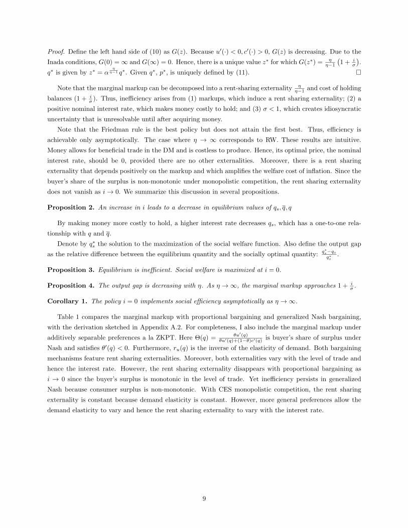
Note that the marginal markup can be decomposed into a rent-sharing externality ηη−1 and cost of holding

balances (1 + iσ ). Thus, inefficiency arises from (1) markups, which induce a rent sharing externality; (2) a

positive nominal interest rate, which makes money costly to hold; and (3) σ < 1, which creates idiosyncratic

uncertainty that is unresolvable until after acquiring money.

Note that the Friedman rule is the best policy but does not attain the first best. Thus, efficiency is

achievable only asymptotically. The case where η → ∞ corresponds to RW. These results are intuitive.

Money allows for beneficial trade in the DM and is costless to produce. Hence, its optimal price, the nominal

interest rate, should be 0, provided there are no other externalities. Moreover, there is a rent sharing

externality that depends positively on the markup and which amplifies the welfare cost of inflation. Since the

buyer’s share of the surplus is non-monotonic under monopolistic competition, the rent sharing externality

does not vanish as i→ 0. We summarize this discussion in several propositions.

Proposition 2. An increase in i leads to a decrease in equilibrium values of qs, q, q

By making money more costly to hold, a higher interest rate decreases qs, which has a one-to-one rela-

tionship with q and q.

Denote by q∗s the solution to the maximization of the social welfare function. Also define the output gap

as the relative difference between the equilibrium quantity and the socially optimal quantity:q∗s−qsq∗s

.

Proposition 3. Equilibrium is inefficient. Social welfare is maximized at i = 0.

Proposition 4. The output gap is decreasing with η. As η →∞, the marginal markup approaches 1 + iσ .

Corollary 1. The policy i = 0 implements social efficiency asymptotically as η →∞.

Table 1 compares the marginal markup with proportional bargaining and generalized Nash bargaining,

with the derivation sketched in Appendix A.2. For completeness, I also include the marginal markup under

additively separable preferences a la ZKPT. Here Θ(q) = θu′(q)θu′(q)+(1−θ)c′(q) is buyer’s share of surplus under

Nash and satisfies θ′(q) < 0. Furthermore, ru(q) is the inverse of the elasticity of demand. Both bargaining

mechanisms feature rent sharing externalities. Moreover, both externalities vary with the level of trade and

hence the interest rate. However, the rent sharing externality disappears with proportional bargaining as

i → 0 since the buyer’s surplus is monotonic in the level of trade. Yet inefficiency persists in generalized

Nash because consumer surplus is non-monotonic. With CES monopolistic competition, the rent sharing

externality is constant because demand elasticity is constant. However, more general preferences allow the

demand elasticity to vary and hence the rent sharing externality to vary with the interest rate.

9

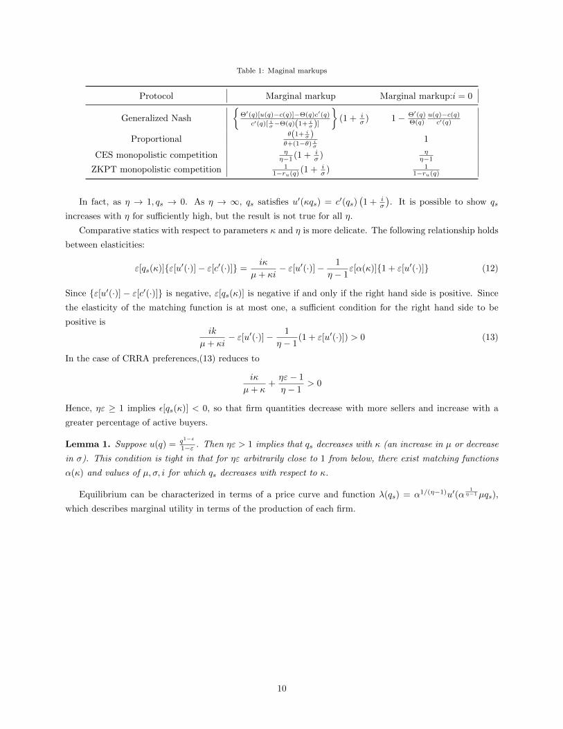
Table 1: Maginal markups

Protocol Marginal markup Marginal markup:i = 0

Generalized Nash

Θ′(q)[u(q)−c(q)]−Θ(q)c′(q)

c′(q)[ iσ−Θ(q)(1+ iσ )]

(1 + i

σ ) 1− Θ′(q)Θ(q)

u(q)−c(q)c′(q)

Proportionalθ(1+ i

σ )θ+(1−θ) iσ

1

CES monopolistic competition ηη−1 (1 + i

σ ) ηη−1

ZKPT monopolistic competition 11−ru(q) (1 + i

σ ) 11−ru(q)

In fact, as η → 1, qs → 0. As η → ∞, qs satisfies u′(κqs) = c′(qs)(1 + i

σ

). It is possible to show qs

increases with η for sufficiently high, but the result is not true for all η.

Comparative statics with respect to parameters κ and η is more delicate. The following relationship holds

between elasticities:

ε[qs(κ)]ε[u′(·)]− ε[c′(·)] =iκ

µ+ κi− ε[u′(·)]− 1

η − 1ε[α(κ)]1 + ε[u′(·)] (12)

Since ε[u′(·)] − ε[c′(·)] is negative, ε[qs(κ)] is negative if and only if the right hand side is positive. Since

the elasticity of the matching function is at most one, a sufficient condition for the right hand side to be

positive isik

µ+ κi− ε[u′(·)]− 1

η − 1(1 + ε[u′(·)]) > 0 (13)

In the case of CRRA preferences,(13) reduces to

iκ

µ+ κ+ηε− 1

η − 1> 0

Hence, ηε ≥ 1 implies ε[qs(κ)] < 0, so that firm quantities decrease with more sellers and increase with a

greater percentage of active buyers.

Lemma 1. Suppose u(q) = q1−ε

1−ε . Then ηε > 1 implies that qs decreases with κ (an increase in µ or decrease

in σ). This condition is tight in that for ηε arbitrarily close to 1 from below, there exist matching functions

α(κ) and values of µ, σ, i for which qs decreases with respect to κ.

Equilibrium can be characterized in terms of a price curve and function λ(qs) = α1/(η−1)u′(α1

η−1µqs),

which describes marginal utility in terms of the production of each firm.

10

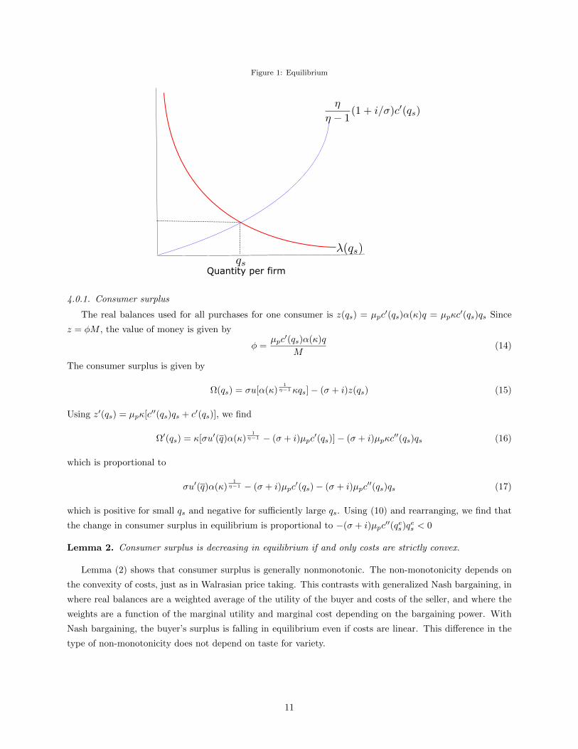
Figure 1: Equilibrium

Quantity per firm

4.0.1. Consumer surplus

The real balances used for all purchases for one consumer is z(qs) = µpc′(qs)α(κ)q = µpκc

′(qs)qs Since

z = φM , the value of money is given by

φ =µpc′(qs)α(κ)q

M(14)

The consumer surplus is given by

Ω(qs) = σu[α(κ)1

η−1κqs]− (σ + i)z(qs) (15)

Using z′(qs) = µpκ[c′′(qs)qs + c′(qs)], we find

Ω′(qs) = κ[σu′(q)α(κ)1

η−1 − (σ + i)µpc′(qs)]− (σ + i)µpκc

′′(qs)qs (16)

which is proportional to

σu′(q)α(κ)1

η−1 − (σ + i)µpc′(qs)− (σ + i)µpc

′′(qs)qs (17)

which is positive for small qs and negative for sufficiently large qs. Using (10) and rearranging, we find that

the change in consumer surplus in equilibrium is proportional to −(σ + i)µpc′′(qes)q

es < 0

Lemma 2. Consumer surplus is decreasing in equilibrium if and only costs are strictly convex.

Lemma (2) shows that consumer surplus is generally nonmonotonic. The non-monotonicity depends on

the convexity of costs, just as in Walrasian price taking. This contrasts with generalized Nash bargaining, in

where real balances are a weighted average of the utility of the buyer and costs of the seller, and where the

weights are a function of the marginal utility and marginal cost depending on the bargaining power. With

Nash bargaining, the buyer’s surplus is falling in equilibrium even if costs are linear. This difference in the

type of non-monotonicity does not depend on taste for variety.

11

5. Entry of sellers

In this section we endogenize the measure of sellers, denoted µ. Given that there is a unit measure of

buyers, µ is also the ratio of sellers to buyers. The dependence of α and αs on µ reflects search externalities.

As µ increases, the measure of sellers per shopper increases: there is a thick market externality (buyers can

purchase a larger share of DM goods) and a congestion externality (each seller is approached by a smaller

measure of buyers). The thick market externality considered here is different from the one in RW where

buyers have a greater probability of being matched. Here, there is an expansion of the measure of matches

(which occur with probability 1). To emphasize this point and more cleanly compare with DS, I abstract

from preference shocks: σ = 1. We compare our results DS, which analyzes the problem of scale versus

diversity with free entry of sellers. I examine the same tradeoff but generalized to a monetary economy with

search frictions between agents. Hence, κ = µ, and the measure of sellers contacted by each buyer is just

α(µ). The CES version of DS arises by setting α(µ) = µ, i = 0, c(·) = c. The first constraint removes search

frictions, the second removes cost of holding real balances, and the third captures scale economies in the

simplest way: a fixed cost and constant marginal cost.

Sellers can choose to enter the market in the following DM by paying a cost a in the current CM. The

cost must be paid each CM period for continued entry. The opportunity cost of entry is thus k = (1 + ρ)a,

where ρ is the discount rate 1−ββ .

The measure of the varieties of the DM good a buyer can purchase is given by α(µ), where α(0) =

0, α′(µ) > 0, α′′(µ) < 0 and α(µ) ≤ µ. Similarly, the measure of buyers for each seller is αs = α/µ, and we

assume limµ→0 αs = 1.11

5.1. Socially efficient allocations

As in the basic model, firms produce the same quantity qs in the social optimum. Using q = α(µ)1/(η−1)µqs,

we can write social welfare as a function of qs and µ:

W (qs, µ) = u[α1/(η−1)µqs]− µ [c(qs) + k] (18)

This is the utility of DM consumption of buyers minus the production cost of the sellers and their entry cost.

The first order conditions are

[qs] α1

η−1u′[α1/(η−1)µqs] = c′(qs) (19)

[µ]k + c(qs)

qsc′(qs)=

[ε[α(µ)]

η − 1+ 1

](20)

where ε[α(µ)] is the elasticity of the matching function with respect to the measure of sellers. Note that the

elasticity is decreasing and bounded above by 1.12

Equation (19) says that the marginal utility of consuming a particular variety equals the marginal costs of

producing that particular variety. Equation (20) characterizes the optimal scale of production. As Dixit and

Stiglitz (1977) stressed, the optimal point of production is not in general at the efficient scale, where average

11A general function that satisfies these conditions is α(µ) = µ

(µb+1)1b

. The elasticity is given by 1µb+1

.

12This follows easily from the concavity of α(·). If f : R+ 7→ R is increasing, differentiable, and concave, then f ′(x∗) ≤ f(x∗)x∗ ,

so thatx∗f ′(x∗)f(x∗) ≤ 1, or ε[f(x)] ≤ 1. Furthermore, xf ′(x)/f(x) is decreasing with x.

12

cost is minimized, because of the value of variety. Here we introduce an important innovation: the optimal

scale depends on the effectiveness of forming new matches out of new sellers. In particular, the optimal

ratio of average cost to marginal cost is given by the elasticity of the matching function with respect to the

measure of sellers divided by η − 1, which reflects the taste for variety, plus unity. Note that for α(µ) = µ

the right hand side equals ηη−1 . Also as η →∞, the socially optimal scale becomes the efficient scale.

The ratio of average to marginal cost is an important quantity, so define Γ(qs) = k+c(qs)qsc′(qs)

. It is straightfor-

ward to show that given µ, the relationship Γ(qs) =[ε[α(µ)]η−1 + 1

]holds for a unique qs(µ). Γ(qs) is decreasing

everywhere, tends to ∞ as qs → 0, and tends to 0 as qs → ∞. Note that this holds even if c(·) = c. Thus

(20) defines an implicit decreasing function qs(µ). It is evident that if there is no taste for variety (η →∞)

and scale economies, then the optimal measure of firms shrinks to zero, as fixed costs are positive.

5.2. Equilibrium

The problem of the buyers and sellers are identical to the basic case except for the new entry margin. In

equilibrium,

k = qsp(j)− c(qs) (21)

Note that, in contrast to RW, qs does not depend on the ratio of sellers to buyers, and thus monetary policy

cannot affect firm size. This will have important implications for optimal policy, as we shall see. Because

sellers face identical problems that admit a unique solution, q(j) = q for all j. This implies q = αηη−1 q. As a

result, the DM output level solves

α1/(η−1)u′[α1/(η−1)µqs]

c′(qs)=

(η

η − 1

)(1 + i) (22)

I define equilibrium for the model with entry.

Definition 2. An equilibrium is a list (p, qs, µ) that solves (10) (modified with σ = 1),(11), and (21).

I reduce equilibrium to a pair of equations for (qs, µ):

Γ(qs) =η

η − 1(23)

α1/(η−1)u′(α1

η−1µqs)

c′(qs)=

η

η − 1(1 + i) (24)

Equation (23) says that in equilibrium average cost is a constant markup over marginal cost. This determines

qs. Equation (24) describes a markup relationship that determines µ given qs. Equilibrium has a recursive

structure. I first determine qs from (23) and then determine µ from qs and (24).

13

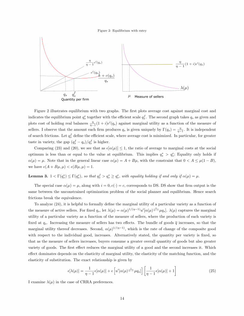
Figure 2: Equilibrium with entry

Measure of sellersQuantity per firm

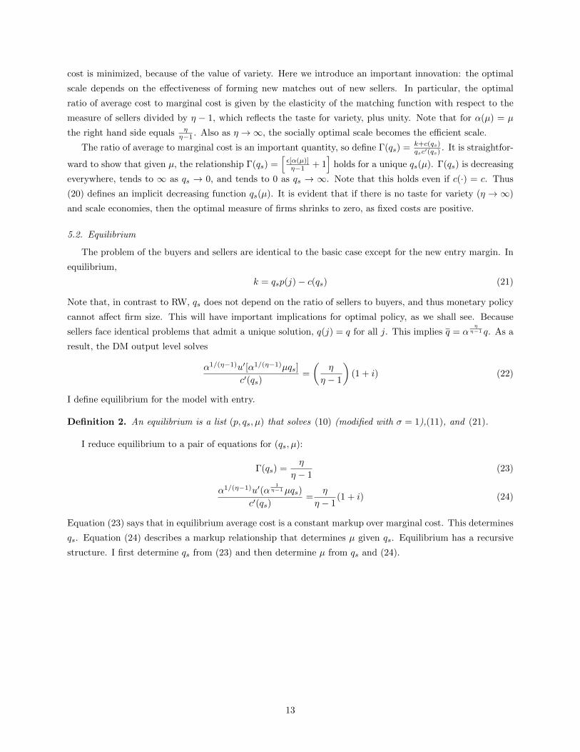
Figure 2 illustrates equilibrium with two graphs. The first plots average cost against marginal cost and

indicates the equilibrium point qes together with the efficient scale qfs . The second graph takes qs as given and

plots cost of holding real balances ηη−1 (1 + i)c′(qs) against marginal utility as a function of the measure of

sellers. I observe that the amount each firm produces qs is given uniquely by Γ(qs) = ηη−1 . It is independent

of search frictions. Let qfs define the efficient scale, where average cost is minimized. In particular, for greater

taste in variety, the gap (qfs − qs)/qfs is higher.

Comparing (23) and (20), we see that as ε[α(µ)] ≤ 1, the ratio of average to marginal costs at the social

optimum is less than or equal to the value at equilibrium. This implies q∗s > qes ; Equality only holds if

α(µ) = µ. Note that in the general linear case α(µ) = A+ Bµ, with the constraint that 0 < A ≤ µ(1− B),

we have ε(A+Bµ, µ) < ε(Bµ, µ) = 1.

Lemma 3. 1 < Γ(q∗s ) ≤ Γ(qes), so that qfs > q∗s ≥ qes, with equality holding if and only if α(µ) = µ.

The special case α(µ) = µ, along with i = 0, c(·) = c, corresponds to DS. DS show that firm output is the

same between the unconstrained optimization problem of the social planner and equilibrium. Hence search

frictions break the equivalence.

To analyze (24), it is helpful to formally define the marginal utility of a particular variety as a function of

the measure of active sellers. For fixed qs, let λ(µ) = α(µ)1/(η−1)u′[α(µ)1

η−1µqs]. λ(µ) captures the marginal

utility of a particular variety as a function of the measure of sellers, where the production of each variety is

fixed at qs. Increasing the measure of sellers has two effects. The bundle of goods q increases, so that the

marginal utility thereof decreases. Second, α(µ)1/(η−1), which is the rate of change of the composite good

with respect to the individual good, increases. Alternatively stated, the quantity per variety is fixed, so

that as the measure of sellers increases, buyers consume a greater overall quantity of goods but also greater

variety of goods. The first effect reduces the marginal utility of a good and the second increases it. Which

effect dominates depends on the elasticity of marginal utility, the elasticity of the matching function, and the

elasticity of substitution. The exact relationship is given by

ε[λ(µ)] =1

η − 1ε[α(µ)] + ε

[u′[α(µ)

1η−1µqs]

] [ 1

η − 1ε[α(µ)] + 1

](25)

I examine λ(µ) in the case of CRRA preferences.

14

Example 1. Let u(·) = q1−ε/(1− ε). Then λ(µ) = α(µ)1−εη−1µ−εq−εs . Hence, ε[λ(µ)] = 1−ε

η−1ε[α(µ)]− ε. Since

ε[α(µ)] is bounded above by 1, ε[λ(µ)] ≤ 1−ηεη−1 .

I state this and some limiting results in a lemma.

Lemma 4. Let u(q) = q1−ε/(1 − ε) for 0 < ε < 1. If ηε > 1 then λ′(µ) < 0. As η → ∞, ε[λ(µ)] → −ε,the elasticity of marginal utility of consumption. As ε → 0 (utility becomes linear in the composite good),

ε[λ(µ)]→ ε[α(µ)]/(η − 1).

In words, as the measure of sellers increase, there is diminishing marginal utility for the marginal good

unless there is sufficiently high taste for variety and/or a high enough elasticity of the marginal utility of the

composite good.

If ηε < 1, then the behavior of the matching function depends on µ, as the following example shows.

Example 2. If α(µ) = µ/(1 + µ), then ε[λ(µ)] = 1−εη−1

11+µ − ε, which is positive for µ sufficiently low if

ηε < 1.

I state results on comparative statics of equilibrium:

Proposition 5. The comparative statics are provided by Table 2.

Table 2: Comparative statics

(a) λ′(µ) < 0

Parameter qs p µ

i 0 0 ↓k ↑ ↑ ↓η ↑ − ↓

(b) λ′(µ) > 0

Parameter qs p µ

i 0 0 ↑k ↑ ↑ ↑η ↑ − ↑

Proof. I examine the comparative statics of equilibrium. Consider an increase in k. Equation (23) shows

that the quantity sold by sellers to all consumers, qs, is increasing. Hence, p = ηη−1c

′(qs) is increasing as

well. Consider now an increase in η. This implies a lower markup. In order for the right hand side of (23) to

remain constant, qs must rise. As we have seen, a rise in qs does not imply a fall in µ. To see the effect on

p, write p = k+c(qs)qs

, for which

∂p

∂qs=qsc′(qs)− [k + c(qs)]

q2s

which is positive for k sufficiently low and negative for k sufficiently high. Hence, it is ambiguous.

Finally, suppose i increases. Then the left hand side of (24) must increase. qs is determined independently

of i, so that µ must adjust. As we have seen, the effect on µ is ambiguous.

To complete the analysis with respect to µ we consider the cases λ′(µ) > 0 and λ′(µ) < 0. Suppose

λ′(µ) < 0. Then µ falls whenever the cost of holding real balances increases. As already shown, increases in

i or k shifts the cost of holding real balances up. Suppose instead that λ′(µ) > 0. Then µ increases whenever

the cost of holding real balances decreases.

15

By (23), (24), necessary conditions for equilibrium to be efficient are

ε[α(µ)] =1 (26)

η

η − 1(1 + i) =1 (27)

Equation (26) says that the elasticity of the matching rate with respect to the sellers equals unity. This is

a version of the Hosios condition (1990),which balances the thick market and congestion externalities. The

entry of a new firm increases the variety of goods for consumes but reduces the buyers of other firms.

As previously, discussed, the matching elasticity is strictly bounded above by unity, so the Hosios condition

cannot be satisfied. Similarly, as η > 1, the second necessary condition is inconsistent.

Proposition 6. Every equilibrium is inefficient.

These inconsistent systems, however, make it clear that the only way a deviation from the Friedman rule

could be welfare improving is by reducing the measure of sellers and thereby raising the elasticity of the

matching function. However, we show in general that the Friedman rule maximizes equilibrium welfare.

Proposition 7. Let (qs, µ) be an equilibrium. Then welfare is maximized at i = 0.

Proof. Consider a social planner who takes qs as given and chooses µ to maximize social welfare. Then we

check that the corresponding i from (24) is never satisfied with i > 0. The planner solves

maxµ

u(α1/(η−1)µqs)− µ[c(qs) + k]

given qs satisfying (23). The first order condition is

u′[α1/(η−1)µqs][1

η − 1α(2−η)/(η−1)α′(µ)µ+ α(µ)1/(η−1)] =

c(qs) + k

qs(28)

In general, (28) is not sufficient. Let µs denote the welfare maximizing root. Using (24) and (23) we write

c(qs) + k

qs=α(µs)1/(η−1)u′(α(µs)1/(η−1)µsqs)

1 + i

Hence we can rewrite (28) in terms of the interest rate as

(1 + i)

[1

η − 1α(µs)(2−η)/(η−1)α′(µs)µs + α(µs)1/(η−1)

]= α(µs)1/(η−1)

This simplifies to

1 + i =η − 1

ε[α(µs)] + η − 1< 1

This is a contradiction because i ≥ 0. This of course results from the fact that we considered a social planner

which can control the measure of sellers directly, whereas the monetary authority can only affect the measure

of sellers by varying the nominal interest rate. The relevant implication is that i = 0 maximizes social

welfare.

The optimality of the Friedman rule contrasts with competitive equilibrium in RW. The essential difference

is that in RW there is a positive probability of sellers paying a fixed cost to enter and not matching with any

buyers. This results in marginal cost exceeding average cost in equilibrium, so that firms operate beyond

16

efficient scale even with no taste in variety.13 Reducing sellers reduces probability of non-trade and brings

trade closer to efficient scale, so inflation may be useful. Hence, the details of search frictions can are

important with respect to the welfare properties of inflation.

5.2.1. Non-monotonicity of consumer surplus

From the basic model, we know that the change in consumer surplus is given by −µ(σ + i)µpc′′(qes)q

es .

Since Γ(qes) = µp, we can rewrite this as

Ω′(qes) = −µe(σ + i)µpc′′[Γ−1(µp)]Γ

−1(µp) (29)

Noting that Γ−1′(µp) = 1Γ′(qs)

> 0, and Ω′(qes) is more negative, provided λ′(µe) < 0. Higher markups

increase qs, which interact with convex costs to make the change in consumer surplus more negative unless

the measure of sellers decreases sufficiently. The behavior of consumer surplus is sensitive to firm entry in

two ways: it depends directly on the measure of sellers, and it depends on quantities provided by each firm

given by (23).

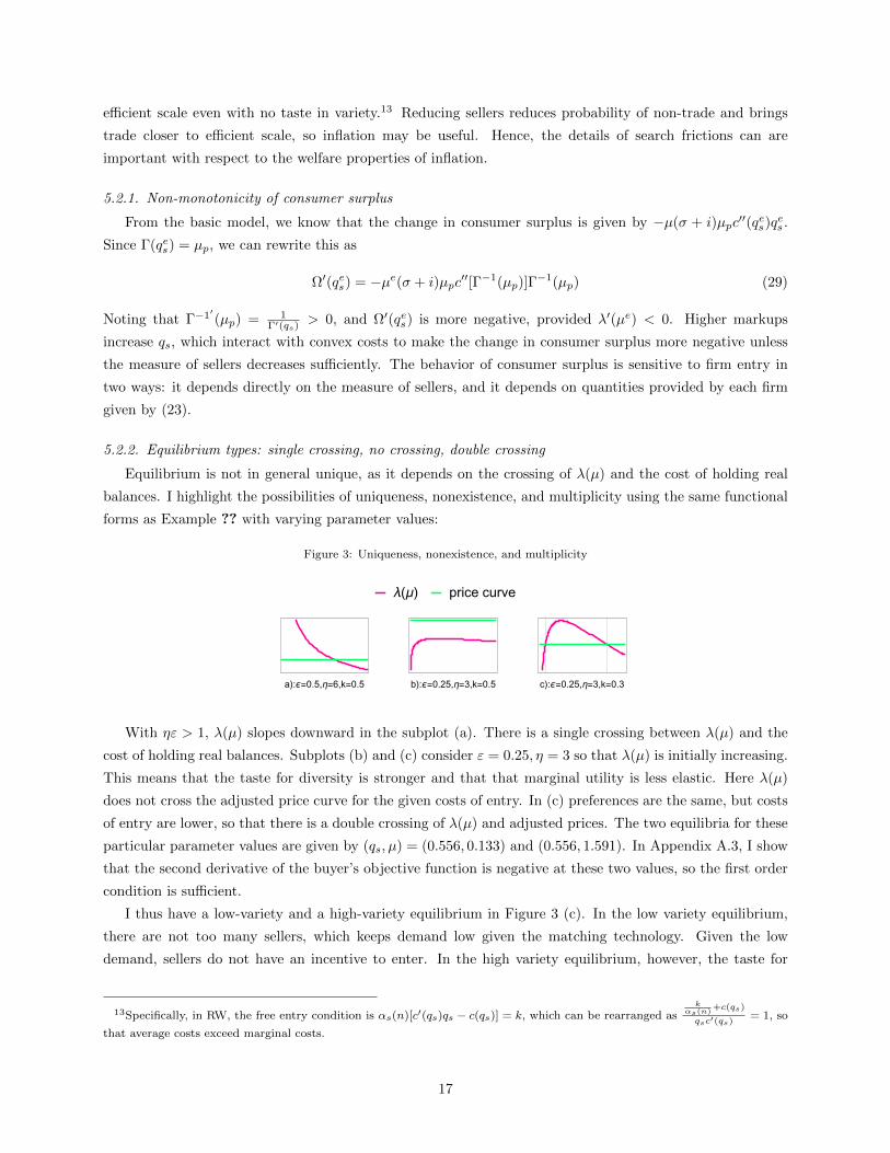
5.2.2. Equilibrium types: single crossing, no crossing, double crossing

Equilibrium is not in general unique, as it depends on the crossing of λ(µ) and the cost of holding real

balances. I highlight the possibilities of uniqueness, nonexistence, and multiplicity using the same functional

forms as Example ?? with varying parameter values:

Figure 3: Uniqueness, nonexistence, and multiplicity

λ(μ) price curve

a):ϵ=0.5,η=6,k=0.5 b):ϵ=0.25,η=3,k=0.5 c):ϵ=0.25,η=3,k=0.3

With ηε > 1, λ(µ) slopes downward in the subplot (a). There is a single crossing between λ(µ) and the

cost of holding real balances. Subplots (b) and (c) consider ε = 0.25, η = 3 so that λ(µ) is initially increasing.

This means that the taste for diversity is stronger and that that marginal utility is less elastic. Here λ(µ)

does not cross the adjusted price curve for the given costs of entry. In (c) preferences are the same, but costs

of entry are lower, so that there is a double crossing of λ(µ) and adjusted prices. The two equilibria for these

particular parameter values are given by (qs, µ) = (0.556, 0.133) and (0.556, 1.591). In Appendix A.3, I show

that the second derivative of the buyer’s objective function is negative at these two values, so the first order

condition is sufficient.

I thus have a low-variety and a high-variety equilibrium in Figure 3 (c). In the low variety equilibrium,

there are not too many sellers, which keeps demand low given the matching technology. Given the low

demand, sellers do not have an incentive to enter. In the high variety equilibrium, however, the taste for

13Specifically, in RW, the free entry condition is αs(n)[c′(qs)qs − c(qs)] = k, which can be rearranged ask

αs(n)+c(qs)

qsc′(qs)= 1, so

that average costs exceed marginal costs.

17

variety induces a higher demand, which is enough to sustain a greater measure of sellers. Note that we

can compare social welfare between the low-variety equilibrium and high-variety equilibrium by comparing

u[α(µ)1

η−1µqs]−µµpc′(qs). Social welfare turns out to be higher in the second case. Since sellers are indifferent

in either equilibrium due to the zero profit condition, the low-variety equilibrium is Pareto inferior to the

high-variety equilibrium. Thus, there is a coordination problem. If a sufficiently great mass of sellers entered,

the extra variety would push up marginal utility and raise demand enough for the sellers to break even.

However, an individual seller has no incentive to enter unilaterally. However, this multiplicity requires very

low elasticity of substitution.

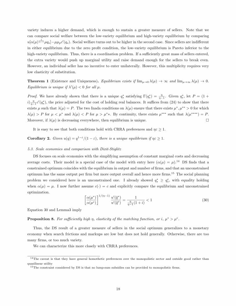
Theorem 1 (Existence and Uniqueness). Equilibrium exists if limµ→0 λ(µ) → ∞ and limµ→∞ λ(µ) → 0.

Equilibrium is unique if λ′(µ) < 0 for all µ.

Proof. We have already shown that there is a unique q∗s satisfying Γ(q∗s ) = ηη−1 . Given q∗s , let P = (1 +

i) ηη−1c

′(q∗s ), the price adjusted for the cost of holding real balances. It suffices from (24) to show that there

exists µ such that λ(µ) = P . The two Inada conditions on λ(µ) ensure that there exists µ∗, µ∗∗ > 0 for which

λ(µ) > P for µ < µ∗ and λ(µ) < P for µ > µ∗∗. By continuity, there exists µ∗∗∗ such that λ(µ∗∗∗∗) = P .

Moreover, if λ(µ) is decreasing everywhere, then equilibrium is unique.

It is easy to see that both conditions hold with CRRA preferences and ηε ≥ 1.

Corollary 2. Given u(q) = q1−ε/(1− ε), there is a unique equilibrium if ηε ≥ 1.

5.3. Scale economies and comparison with Dixit-Stiglitz

DS focuses on scale economies with the simplifying assumption of constant marginal costs and decreasing

average costs. Their model is a special case of the model with entry here (α(µ) = µ).14 DS finds that a

constrained optimum coincides with the equilibrium in output and number of firms, and that an unconstrained

optimum has the same output per firm but more output overall and hence more firms.15 The social planning

problem we considered here is an unconstrained one. I already showed q∗s ≥ qes , with equality holding

when α(µ) = µ. I now further assume c(·) = c and explicitly compare the equilibrium and unconstrained

optimization. [α(µ∗)

α(µe)

]1/(η−1)u′(q∗)

u′(qe)=

1ηη−1 (1 + i)

< 1 (30)

Equation 30 and Lemma3 imply

Proposition 8. For sufficiently high η, elasticity of the matching function, or i, µ∗ > µe.

Thus, the DS result of a greater measure of sellers in the social optimum generalizes to a monetary

economy when search frictions and markups are low but does not hold generally. Otherwise, there are too

many firms, or too much variety.

We can characterize this more closely with CRRA preferences.

14The caveat is that they have general homothetic preferences over the monopolistic sector and outside good rather than

quasilinear utility15The constraint considered by DS is that no lump-sum subsidies can be provided to monopolistic firms.

18

[α(µ∗)

α(µe)

] 1−εη−1

[µ∗

µe

]ε =

(q∗sqes

)ε1

µp(1 + i)(31)

The comparison between µ∗ and µe depends on whether the right hand side exceeds 1. Suppose ηε > 1. If

the right hand side exceeds 1 then µ∗ > µe. Otherwise, µ∗ < µe. In the frictionless benchmark, α(µ) = µ,

and using qes = q∗s we obtainµ∗

µe= [µp(1 + i)]

η−1ηε−1

In the case of frictionless matching, ηε > 1 implies µ∗ > µe. With search frictions, it depends on whether the

right hand side exceeds 1. There is no general way to bound q∗s/qes because it becomes arbitrarily large as

ε[α(µ)]η−1 → 0, which can happen if the elasticity of the matching function approaches zero or as goods become

perfectly substitutable. In that case, it is socially optimal to have very few sellers producing many goods.

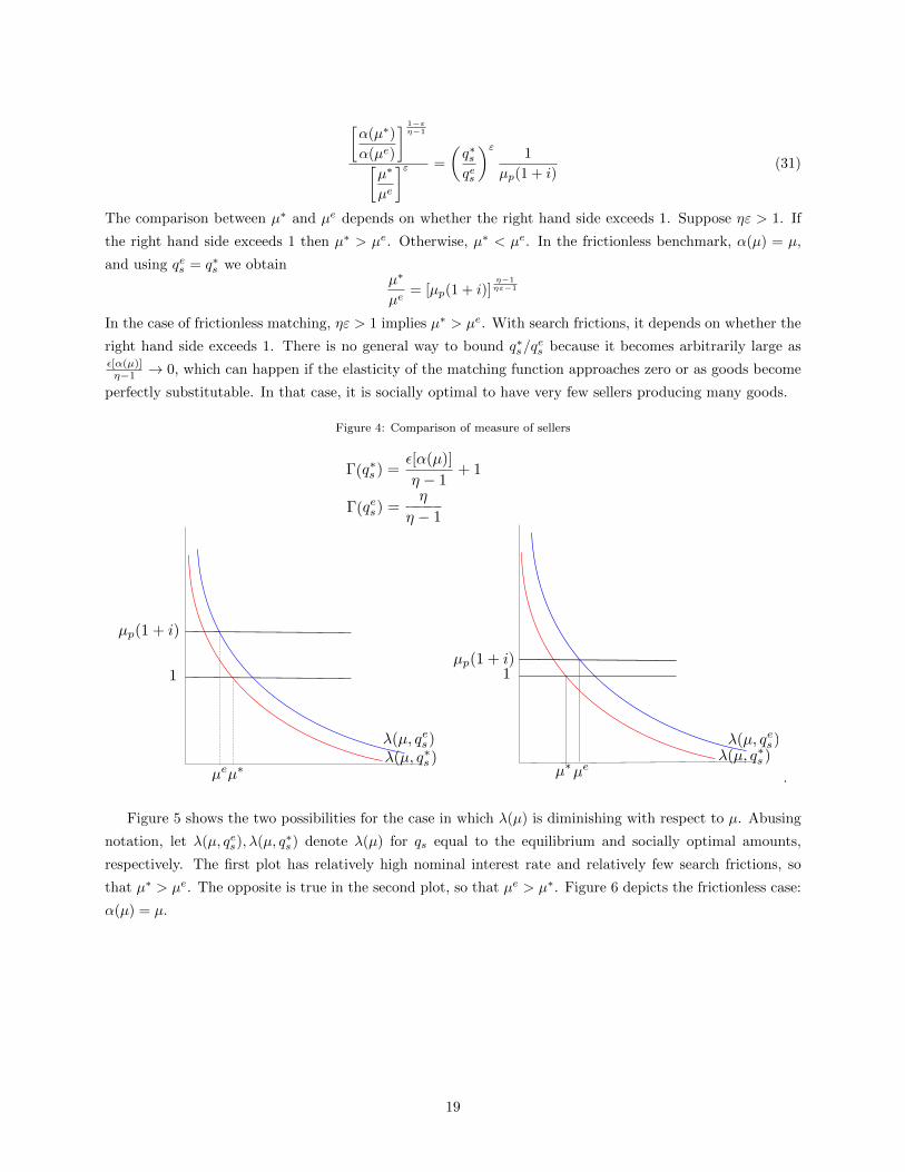
Figure 4: Comparison of measure of sellers

.

Figure 5 shows the two possibilities for the case in which λ(µ) is diminishing with respect to µ. Abusing

notation, let λ(µ, qes), λ(µ, q∗s ) denote λ(µ) for qs equal to the equilibrium and socially optimal amounts,

respectively. The first plot has relatively high nominal interest rate and relatively few search frictions, so

that µ∗ > µe. The opposite is true in the second plot, so that µe > µ∗. Figure 6 depicts the frictionless case:

α(µ) = µ.

19

Figure 5: Comparison of measure of sellers: α(µ) = µ

.

In this case, there is no congestion externality, but there is reduced demand from both the inflation wedge

and price markups. Hence, µ∗ > µe. The case considered in DS arises simply from setting i = 0, in which

case price markups would be the only inefficiency.

6. Variable markups and the role of complementarity

I emphasized CES preference because of simplicity and to facilitate comparison with Dixit Stiglitz. But

there are well known problems with CES. Zhelobodko, Kokovin, Parenti, and Thisse (2012), hearafter ZKPT,

identify two important deficiencies: (1) markups and prices are independent of firm entry and market size

and (2) the lack of a scale effect (the size of firms and markups are independent of the number of consumers).

The free entry of sellers makes (1) particularly salient in this context. Furthermore, the marginal utility

of a variety u′(q)α(µ)1

η−1 decreases with fewer sellers because of complementarity, yet there is no change

in markup. We investigate the importance of these channels by relaxing complementarity with additively

separable preferences and introducing variable markups. This enables us to decompose the change in welfare

costs of inflation into (1) complementarity effects and (2) variable markup effects.

Variable markups require changing the preferences, and we adopt additively separable preferences over

varieties a la ZKPT in the DM.

6.1. The buyer’s problem

The preferences of the buyer in the DM are given by∫ Ω

0

u(qi)di (32)

where Ω is the potential set of varieties. Hence, the period utility function of the buyer is given by

U b(x, h, q(j)) =

∫ Ω

0

u(qi)di+ U(x)− h (33)

where u(0) = 0, u′(0) =∞, u′(q) > 0, and u′′(q) < 0 for q > 0. U(·) satisfies the same conditions as u(·).

20

The concavity of u(·) reflects taste for variety. Consumers prefer to spread consumption over all varieties

than a small mass of varieties. There is a formal equivalence between decision-making by consumers with

taste for variety and the Arrow-Pratt theory of risk aversion. Consumers’ taste for variety can be measured

from the relative love for variety (RLV)

ru(q) = −qu′′(q)

u′(q)> 0 (34)

which is the familiar elasticity of marginal utility, or inverse of elasticity of substitution in the case qi = q ∀i.Preferences which display an increasing RLV mean that consumers perceive varieties as being less substi-

tutable when they consume more. Preferences may also display a decreasing RLV and be more substitutable

with higher consumption. We assume ru′(q) < 2 ∀q > 0, which we shall see makes the producers’ problem

concave.

Figure 6

0.0 0.5 1.0 1.5 2.00.0

0.2

0.4

0.6

0.8

1.0Relative love for variety

q1-ϵ

1-ϵ

q1-ϵ

1-ϵ+B q

q1-ϵ

1-ϵ-B q

1-exp[-γ q]

q

2+2 log[1+q]

Figure 6 depicts the RLV for several functional forms.

The problem for the buyer is given by

maxqi

∫ α(µ)

0

u(qi)di− (1 + i)z

(35)

where z =∫ α(µ)

0piqidi as before. The solution is given by

u′(qi) = (1 + i)pi (36)

where an interior solution is guaranteed because of the Inada condition. pi(qi) is strictly decreasing because

u(·) is strictly concave. The elasticity of the inverse demand εp(qi) and the price elasticity of demand are

related to the RLV as1

εq(p)= εp(q) = ru(q) (37)

Hence, the price elasticity of demand is just the reciprocal of the RLV. This implies that RLV increases if

and only if demand for a variety becomes less elastic with quantity (more elastic with price). Intuitively,

consumers are less willing to substitute goods with higher consumption. Hence, as with CES, taste for variety,

elasticity of substitution, and price elasticity of demand are interchangeable, but in contrast to CES they

depend on the consumption level of qi.16

16The preceding is a special case of the discussion in Mrazova and Neary (2013). Elasticity of demand decreases with sales

21

Furthermore, suppose that there are more available varieties, and consumers spread out consumption

among the greater set of varieties. Then q is lower for each variety, so that with increasing RLV, ru(q) is lower.

Hence, there is more substitutability between varieties. This confirms the intuition that the substitutability

of varieties increases with the number of varieties, all else constant.

6.2. The producers’ problem

The producer j produces qj for measure αs = α(κ)κ consumers. As before, let qs(j) = αsq(j)

maxpj ,qjp(j)qs(j)− c(qs) (38)

where p(j) is given by (36). The solution equates marginal revenue u′(q)[1−ru(q)]1+i to marginal cost c′(qs), and

yields

ru(qi) =u′(qi)− (1 + i)c′(qs)

u′(qi)(39)

Notice that the right-hand side of (39) is equal to the net markup. Hence, with µ given, a firm chooses qs

such that the markup equals the RLV. Furthermore, ru(q) < 1 (firm produces in the elastic region).

The solution is unique provided the profit function is concave. Differentiating (39) with respect to qi,

dividing by u′(qi), and rearranging shows that the second order condition is equivalent to

[2− ru′(qi)]ru(qi)− [1− ru(qi)]rc(qs) > 0 (40)

where rc = −qc′′/c′ is the negative elasticity of marginal cost. By construction, rc < 0, so that the second

term in (40) is positive. ru′(qi) measures the convexity of demand for qi, so the second order condition requires

that demand not be too convex. ru′(qi) < 2 ∀q ≥ 0 is sufficient because the second term is nonnegative.

Note that, in the CES case u(q) = q1−ε

1−ε , ru = ε, and ru′ = 1 + ε, so that ε < 1 is a sufficient condition.

The condition that marginal revenue equals marginal cost can be expressed as p(qs) + qsp′(qs) = c′(qs),

which implies that p−c′(qs)p(qs)

= − qsp′(qs)

p(qs)= 1

εp(qs). Hence, an increase in marginal cost c, which must lower

sales, is associated with a higher elasticity. It is useful to define the curvature of demand ξ(q) = − qp′′(q)p′(q) .

Following Mrazova and Neary (2013), by differentiating the firm FOC with respect to c′(qs),dpdc′ = 1

2−ξ , which

implies dpdc′ − 1 = ξ−1

2−ξ . Hence, there is more than 100% pass-through of costs to prices if and only if ξ > 1.

As the model with entry, producers enter in the CM at cost k up to the point until profits are zero:

k + c(qs) = p(j)qs (41)

Since each seller faces the same problem, which is concave and thereby admits a unique solution, qi = q ∀i.An equilibrium can be defined as prices p, quantities (qs, q), and measure of sellers µ which satisfy

Γ(qs) =1

1− ru(q)(42)

u′(q)

c′(qs)=

1 + i

1− ru(q)(43)

p =c′(qs)

1− ru(q)(44)

qs =α(κ)

κq (45)

if and only if the inverse demand p(q) is subconvex, which means that log p(q) is concave in log q. Alternatively, demand is

superconvex if elasticity of demand increases with sales. These notions will be important for the producers’ problem.

22

Since ru(q) is also the net markup, this means that the ratio of average to marginal costs equals the gross

markup in equilibrium.

Equilibrium can be described in (p, q) space in terms of the following equations:

p =u′(q)

1 + i(46)

p =c′[φ(q)]

1− ru(q)(47)

(48)

where φ(q) = Γ−1

[1

1− ru(q)

]and satisfies φ′(q) < 0. Equation (46) is a demand curve, which depends on

the cost of holding money, and Equation (47) is price setting rule, which reflects the markup directly and

also indirectly via the effect on marginal costs expressed by c′[φ(q)].

Figure 7: Free entry equilibrium with variable markups

p

q

Existence and uniqueness of equilibrium holds generally.

Proposition 9. Equilibrium exists and is unique.

Proof. First, we show that there is a unique crossing of demand and the price setting rule. It suffices to show

that u′(q)[1−ru(q)](1+i)c′[φ(q)] = 1 for unique q. The denominator is increasing and strictly bounded below by zero. The

numerator approaches zero because limq→∞ u′(q) = ∞ and ru(q) < 1 from firm optimization. This defines

unique values p∗ and q∗. In turn, q∗s = φ(q∗) and µ∗ is defined implicitly from q∗s = α(µ∗)µ∗ q∗

Note that, in contrast to CES preferences, the Inada conditions on u(·) suffice for existence and uniqueness

because there is a lack of strategic complementarity of varieties: having more varieties does not increase the

marginal utility of a particular variety. Hence, the marginal utility of a variety approaches zero as the number

of sellers approaches infinite without any further assumptions.

We show that higher interest rates lead to lower overall consumption and larger and fewer firms.

Lemma 5. If r′u(q) > 0 in the neighborhood of equilibrium, then a small increase in i leads to higher qs,

lower q, lower µ, and lower markups.

Proof. An increase in i shifts demand downward and does not change the price setting rule, resulting in lower

p and q. Hence, markups ru(q) are lower. qs = φ(q) is higher. The measure of sellers satisfies α(µ)µ = φ(q)

q .

The right hand side is higher, so that µ is lower.

23

It may seem counterintuitive there can be lower markups with fewer firms. The reasoning is as follows. A

higher nominal interest rate makes it more costly to use money, lowering consumption. Lower demand leads

to lower sales and lower markups on those sales since the taste for variety is lower. Hence, fewer firms enter.

Lemma 6. If r′u(q) > 0 in the neighborhood of equilibrium, then a small decrease in k leads to higher q,

lower qs, higher µ, and higher markups.

Proof. Lower k implies a rightward shift of the supply curve. This can be seen from the fact that Γ is shifted

down and hence φ is shifted up, so that qs = φ(q) is lower (φ is negative). Hence firms have lower marginal

costs c′(φ(q)). Demand is unaffected, so equilibrium occurs at higher q and lower p. Thus, ru(q) and markups

are lower. qsq is lower, so more sellers enter.

Table 3: Comparative statics: r′u(q) > 0

Parameter qs q ru(q) µ

↑ i ↑ ↓ ↓ ↓↑ k ↑ ↓ ↓ ↓

In Figure 8, we consider a rise from i = 0 to i = 0.13 for u(q) = q1−ε

1−ε +Bq, so that ru(q) = ε1+Bqε . This

leads to a sharp decrease in q and increase in qs, reducing welfare significantly.

Figure 8: A rise in the nominal interest rate

6.2.1. Social welfare

The social welfare function can be written as

W (qs, µ) = α(µ)u(q)− µ[k + c(qs)] (49)

24

which has first order conditions17

u′(q) = c′(qs) (50)

Γ(qs) = εα(µ)

(1

εu(q)− 1

)+ 1 (51)

This is a generalization of a result in Vives (1999). Without search frictions, note that Γ(qs) = 1εu(q) , or

εTC(qs) = εu(q), which is the result in Vives (1999). More generally, the optimal deviation of average costs

from the efficient scale increases with a more concave utility function and a less concave matching function.

Comparing (50)-(51) to (42) and (43), we find the one-way comparison q∗s < qes ⇒ q∗ > qe and henceq∗sq∗ <

qesqe ⇔ µ∗ > µe. Thus, as in DS with variable elasticity of demand, if optimal firm size is smaller then the

optimal number of firms is greater. Note that the relationship between q∗s an qes can go either way, because

the former depends on the elasticity of utility and the elasticity of the matching function whereas the latter

depends on the elasticity of demand. Compared to DS, however, qes is higher if i > 0 because of the inflation

wedge and q∗s is lower because the social planner takes into account search frictions.

Proposition 10. Equilibrium is inefficient.

Proof. From (50)-(51) and (46)-(47), necessary and sufficient conditions for equilibrium to implement the

social optimum are 1+i1−ru(q) = 1 and 1−ru(q) = ε[u(q)]

ε[α(µ) . This requires i = 0, ru(q∗) = 0 and ε[u(q∗)] = ε[α(µ∗)].

But ru(q) = 0 is inconsistent with firm optimization. Hence, equilibrium is inefficient.

However, the Friedman rule is not necessarily optimal, as Figure 9 demonstrates.

Figure 9: Social welfare

In this example, social welfare is maximized at i = 0.0173, 0.0361, and 0.0303 across subpanels a),b), and

c), respectively. There are two benefits of inflation in equilibrium. It reduces price markups, and it reduces

average costs of production. The reduction of price markups mitigates the inefficiency on the intensive

margin. Higher inflation reduces product variety, but this is less important for welfare when product variety

is already very high. A lower level or higher elasticity of costs shift the optimal nominal interest rate higher.

It is instructive to compare this optimal deviation from the Friedman rule to that of competitive equilibrium

in RW. Inflation there reduces sellers and hence reduces congestion, which in turn lowers average costs by

increasing the probability that sellers match with buyers. Here, lower congestion does not reduce average

costs directly. Instead, average costs decrease because markups decrease. The reduction in average costs here

rests on variable elasticity of demand, whereas in RW it results from the matching technology.

17For (51) we obtain α′(µ)u(q) + u′(q)[1− εα(µ)]qs = k + c(qs) using ∂q∂qs

=1−εα(µ)α(µ)

. Then we divide both sides by qsc′(qs)

and use the fact that u′(q) = c′(qs) and rearrange in terms of εα, εu, and Γ.

25

Inflation hence reduces sellers’ market whenever ru is increasing. The idea that inflation can reduce

sellers’ market power is not new. In Diamond (1993) or in a basic new Keynesian model, inflation reduces

markups with sticky prices, but here the result instead results from changes in equilibrium taste of variety

and without any nominal rigidity.

The ratio of average costs to marginal costs in the social optimum and equilibrium are given by Γ(q∗s ) =ε[α(µ)]ε[u(q)] and Γ(qes) = 1

1−ru(q) . In words, the socially optimal quantity is uniquely determined by the elasticity

of utility and elasticity of the matching, whereas the equilibrium quantity is determined by the elasticity of

demand (or equivalently the RLV). In general, firms can be either too big or too small relative to the social

optimum.

6.2.2. The elasticity of the markup and augmented HARA preferences

Taking ru(q) = −u′′(q)qu′(q) , applying logs and differentiating, we obtain the elasticity of the markup:

εru = 1 + ru(q)− ξ(q) (52)

where ξ(q) ≤ 2. This says that the elasticity of the markup equals the gross markup minus the curvature

of demand. Since ru(q) = 1εp(q) , the elasticity of the markup is the negative elasticity of the elasticity of

demand. One major task for calibration and estimation is the identification of a suitable choice of utility

functions. In the working paper by ZKPT (2012), the authors consider a an extension of HARA preferences

that is consistent with both increasing and decreasing taste of variety. They dub it ‘augmented HARA’:

u(q) = 1ρ [(a + hq)ρ − aρ] + bq, where a ≥ 0, h ≥ 0, b ≥ 0, 0 < ρ < 1. CES arises with a = b = 0, and HARA

arises with b = 0.18 Furthermore, a > 0 bounds the marginal utility at zero consumption.

RLV takes the form ru(q) = h2(1−ρ)(a+hq)ρ−2qh(a+hq)ρ−1+b . With a = 0, as we wish to include an Inada condition, this

becomes ru(q) = (1−ρ)hρqρ−1

hρqρ−1+b . A crucial question regards the behavior of the elasticity of the taste of variety

(elasticity of markups in equilibrium). Denoting this by εru , we have

εru =(ρ− 1)b

hρqρ−1 + b(53)

For augmented HARA preferences, ξ(q) = (2−ρ)hqa+hq , which is positive and increasing unless a = 0. At a = 0,

this simplifies to 2− ρ. Hence, at a = 0, εru = ρ− 1 + ru(q), which is increasing with q for r′u > 0.

7. Optimality of Friedman rule

Table 4 summarizes the optimality properties of the Friedman rule under various market structures.

Here, ‘first best’ refers to the implementation of the social planning problem, and ‘second best’ refers to the

maximization of equilibrium welfare. For the first four market structures, I refer to the analysis in Rocheteau

Wright (2005). The next two are from the variety model in Dong (2010). The last three are the subject of

this paper.

18If b = 0, the coefficient of absolute risk aversion satisfies −u′′(q)u′(q) =

h(ρ−1)1+hq

, which is hyperbolic. Furthermore, ru(q) is

decreasing for a > 0 and constant for a = 0. This explains the need to modify HARA to be consistent with increasing RLV.

26

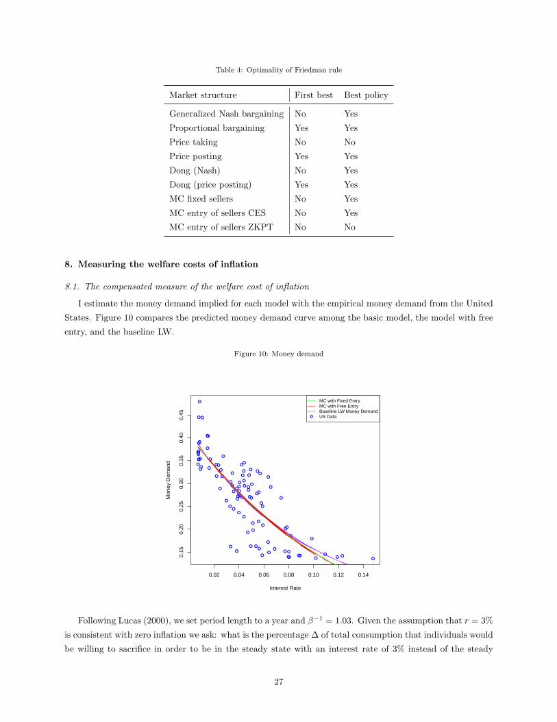
Table 4: Optimality of Friedman rule

Market structure First best Best policy

Generalized Nash bargaining No Yes

Proportional bargaining Yes Yes

Price taking No No

Price posting Yes Yes

Dong (Nash) No Yes

Dong (price posting) Yes Yes

MC fixed sellers No Yes

MC entry of sellers CES No Yes

MC entry of sellers ZKPT No No

8. Measuring the welfare costs of inflation

8.1. The compensated measure of the welfare cost of inflation

I estimate the money demand implied for each model with the empirical money demand from the United

States. Figure 10 compares the predicted money demand curve among the basic model, the model with free

entry, and the baseline LW.

Figure 10: Money demand

0.02 0.04 0.06 0.08 0.10 0.12 0.14

0.15

0.20

0.25

0.30

0.35

0.40

0.45

Interest Rate

Mon

ey D

eman

d

MC with Fixed EntryMC with Free EntryBaseline LW Money DemandUS Data

Following Lucas (2000), we set period length to a year and β−1 = 1.03. Given the assumption that r = 3%

is consistent with zero inflation we ask: what is the percentage ∆ of total consumption that individuals would

be willing to sacrifice in order to be in the steady state with an interest rate of 3% instead of the steady

27

state associated with r (Craig and Rocheteau 2006). I use three observables: money stock (M), nominal

GDP (PY), and the nominal interest rate, which are taken from the dataset by Ireland (2009), compiled from

several different sources. The time range is from 1900-2006. Empirical money demand is defined as M/PY .

i is measured as the short-term commercial paper rate and M1RS is the measure of money demand. 19

I use the same functional forms as Craig and Rocheteau (2006): c(q) = q and u(q) = q1−ε

1−ε . I also take

U(x) = A ln(x) in the CM and the matching function α(µ) = µ/(1 + µ). For the basic model,we normalize

µ = 1 so that α = 12 .

I use the money demand data to match the first four moments of money demand for different values of

η. Estimation is with respect to (ε,A) in the basic model and (ε,A, k) in the free entry model. We calculate

the cost ∆ of 10% inflation, which corresponds to r = 0.03. The formulas for ∆ are given by the following.

In the basic model, sellers make equilibrium profits, which we distribute back to the buyers without loss of

generality because of quasilinear utility. With entry, equilibrium profits are zero. Furthermore, we rewrite

the αq units purchased by the buyer in the DM as α−1

η−1 q.

q0.031−ε

1− ε(1−∆)1−ε +A ln(1−∆)− η

η − 1α−

1η−1 q0.03 =

qr1−ε

1− ε− η

η − 1α−

1η−1 qr (54)

q0.031−ε

1− ε(1−∆)1−ε +A ln(1−∆)− η

η − 1α(µ0.03)−

1η−1 q0.03 =

qr1−ε

1− ε− η

η − 1α(µr)

− 1η−1 qr (55)

For additively separable preferences, the welfare cost ∆ is given by

α(µ0.03)u[q0.03(1−∆)] +A ln(1−∆)− α(µ0.03)q0.03c′(qs,0.03)

1− ru(q0.03)= α(µr)u(qr)− α(µr)qr

c′(qs,r)

1− ru(qr)(56)

Table 5: Welfare costs of inflation

no entry entry

µp ∆ ε A ∆ ε A k

1.01 0.0190 0.0578 0.9857 0.0184 0.0734 1.0324 0.0174

1.05 0.0282 0.0578 0.3328 0.0282 0.0908 0.5353 0.0250

1.1 0.0388 0.0578 0.0885 0.0403 0.1220 0.3805 0.0323

1.2 0.0571 0.0578 0.0069 0.0528 0.2278 0.2776 0.1257

1.3 0.0724 0.0578 0.0006 0.0925 0.2527 0.1954 0.0927

From Table 5 the calibration satisfies ηε > 1, so that λ(µ) is decreasing everywhere and equilibrium

is unique. Free entry makes a substantial difference in the estimated values of ε and A that best fit the

money demand moments. Furthermore, there is little divergence in the welfare costs of inflation between

the no-entry and free-entry cases until markups reach 30% in the decentralized market, at which point free

entry is responsible for a full 2 percentage point increase with respect to the no entry case. The economic

19The M1RS aggregate is defined and constructed by Dutkowsky and Cynamon (2003) and Cynamon, Dutkowsky, and Jones

(2006) by correcting for a bias in M1 from the growth of retail deposit sweep programs, in which banks reclassified part of

checkable deposits as money market deposits to avoid statutory reserve requirements.

28

rationale is that inflation reduces entry, which in equilibrium reduces both variety and also reduces the value

of existing varieties due to the complementarity effect.

At µp = 1.01, taste of variety and markups are very low, so the economy resembles Walrasian price taking.

It is instructive to compare this to Rocheteau Wright (2009), who found welfare costs of inflation at 1.54%

without entry and 1.65% with entry. These values are slightly lower but comparable to the present case. Two

important differences are that without markups they need to introduce some convexity in costs; specifically,

they set δ = 1.1 in c(q) = qδ/δ, and that there is still some small taste for variety and market power in our

case.

9. Conclusion

In this paper, I examined the implications of product variety and multilateral matching for firm size,

variety, and the welfare costs of inflation. Markups amplify the costs of holding real balances through a rent

sharing externality but also help induce entry. Firms produce too little under CES (with or without entry).

Furthermore, with entry, there can either be too many or too few firms relative to the social optimum, and

are likely to be too few with a higher nominal interest rate, a more elastic matching function, and lower taste

for variety. With and without entry, the Friedman rule is best policy with CES preferences and attains first

best as η →∞. The estimated welfare costs of inflation under CES are 7% without entry and over 9% with

entry at 30% markups This is much higher than previous estimates by Lucas (2000) and LW. It is in line

with the highest estimates of RW (2009) and Dong under bargaining. Furthermore, the Friedman rule is not

generally optimal with variable elasticity of demand because inflation reduces markups and, in turn, average

costs. This effect also attenuates the inefficiency on the intensive margin. However, the Friedman rule is

still optimal at parameter values obtained from matching money demand. In the appendix, I also extend the

model to variable search intensity and show that the hot potato effect (rising search intensity to inflation)

identified by LLW requires implausible parameter values if there is congestion in search. This, of course, does

not negate the existence of the hot potato effect, but highlights the importance on the role of congestion on

search intensity.

There are many fruitful directions for further research. For one, the estimates from the welfare cost of

inflation derived from the model are likely upward biased from at least two different reasons. Notably, the

framework rests on a pure monetary economy, but credit provides another means of payment and thereby

mitigates the inflation wedge. Second, markups reasonably result from reasons besides taste for variety,

such as imperfect intermediate goods markets (as in a canonical new Keynesian model). Hence, a reasonable

extension is to modify the model with money and credit, with limited commitment or enforcement constraints,

and have an intermediate goods sector. Furthermore, more general specifications of variable markups can be

used to incorporate degrees of complementarity.

29

Appendix A. Appendix

Appendix A.1. Endogenous search intensity

Appendix A.1.1. Environment

I extend the model by endogenizing buyers’ search for sellers. The main motivation is to understand

how shopping effort and output varies in response to interest rates and compare to LLW. LLW, also using

a flexible labor market, find that with enough substitutability of labor and goods in preferences, inflation

increases and labor, search effort, and output increase if taste for variety is high enough. In contrast to LLW,

we consider the congestion effect of search. I find that though it is possible for effort to rise in response to

interest rates, it requires the taste for variety to be implausibly high relative to the elasticity of the marginal

utility of consumption. Typically, we will see that effort falls modestly.

The measure of overall matches is given by α(e), where

e =

∫ 1

0

e(i)di (A.1)

The measure of varieties of the DM good that a buyer can purchase is given by αb = eα(e)/e. Since buyers

can match up with at most measure µ sellers, α(e) ≤ µ. The measure of buyers for each seller is αs = α(e)/µ.

I assume lime→∞ αs(e) = 1

The aggregate good is a function of the measure of contacted sellers, and hence a function of effort

q(e) =

(∫ eα/e

0

q(j)η−1η dj

) ηη−1

Effort yields disutility given by ψ(e), where ψ′(e) > 0, ψ′′(e) > 0 and ψ(0) = ψ′(0) = 0. The buyer’s period

utility function becomes U b(x, h, q, e) = u(q)− ψ(e) + U(x)− h.

Though we do not explicitly introduce a labor-leisure tradeoff as LLW do, we proxy one via the convexity

of ψ(e).

Appendix A.1.2. Equilibrium

The feasibility constraint on the transfer of real balances∫ eα/e

0p(j)q(j)dj ≤ z is binding and the buyer’s

problem is expressible as

maxq(j),e

−(1 + i)

∫ eα/e

0

p(j)q(j)dj − ψ(e) + u(q)

The first order condition with respect to q(j) is

(1 + i)p(j) = u′(q)

[q

q(j)

]1/η

(A.2)

as before.

The first order condition with respect to effort is:

u′(q)

(η

η − 1

)[q

q(j)

]1/η

qα

e− ψ′(e)− (1 + i)p(j)q(j)

α

e= 0

This can be simplified using (A.2) into

ψ′(e) =(1 + i)p(j)q(j)α/e

η − 1(A.3)

30

Equation (A.3) says that the marginal cost of effort is equal to the marginal utility of effort. Note that

(A.3) reflects a ‘hot potato’ effect. A higher interest rate raises the cost of holding unused real balances and

thereby raises search intensity among buyers. However, this is a partial equilibrium effect. I later show that

in general equilibrium effort is likely to fall due to congestion.

The interpretation of (A.3) is as follows. An extra unit of effort enables the buyer to access α/e extra

sellers and hence αe q(j) extra units. These extra units cost (1 + i)p(j) each, which equals their marginal

benefit by (A.2). Since the right hand side is positive and does not depend on e, and since ψ′(e) > 0 with

ψ′(0) and ψ′(∞) = ∞, there is a unique value of e that solves (A.3). As all buyers face the same problem,

e = e.

The problem of seller j is identical to the basic case except that now qs(j) = αs(e)q(j). Similarly, as

buyers face the same problem with a unique solution,q(j) = q for all j and q = αη/(η−1)q. I are now ready

to define equilibrium.

Definition 3. An equilibrium for the model with endogenous search intensity is a list (qs, e) such that

α(e)1/(η−1)u′[α(e)1/(η−1)µqs]

c′(qs)=

η

η − 1(1 + i) (A.4)

eψ′(e) =η

(η − 1)2c′(qs)µqs(1 + i) (A.5)

I prove existence of equilibrium.

Theorem 2 (Existence and uniqueness). There exists a unique equilibrium.

Proof. Fix e in (0,∞). This fixes α(e) ∈ (0, 1). By the standard argument, tending qs → 0 tends the left

hand side of (A.4) to ∞, and tending qs → ∞ tends the left hand side to 0. By the intermediate value

theorem, there is a (positive) qs such that (A.4) holds. Given that the left hand side is decreasing in qs, this

value is unique. By the implicit function theorem, this defines a differentiable function qs = f(e) such that

f ′(e) < 0. Moreover, using the fact that as e → ∞, α/µ → 1, we have lime→∞ f(e) is given by the unique

value q∞s . Also, lime→0 f(e) =∞.

From (A.5), define the function

g(e) = eψ′(e)− η(1 + i)

(η − 1)2c′[f(e)]µf(e)

It suffices to show that there is a unique e > 0 such that g(e) = 0. As f ′(e) < 0, g′(e) < 0. Furthermore, as

e → ∞, f(e) → q∞, so that g(e) → ∞. Second, note that g(e) → −∞ as e → 0. As e → 0, f(e) → ∞. By

the intermediate value theorem, there is a unique e∗ > 0 such that g(e∗) = 0.

I can describe equilibrium in terms of two curves relating e and qs. Equation (A.4) is the marginal markup

condition. (A.5) describes the effort as a function of firm output. Specifically, there is a linear relationship

between the semi-elasticity of effort cost and the semi-elasticity of production cost.

I derive a necessary and sufficient condition for effort to fall in equilibrium with respect to interest rates.

I take the logarithmic transforms of (A.4) and (A.5), totally differentiate with respect to 1+ i, and rearrange:

ε[e(1 + i)] =1 + ε[u′(·)]

[1 + ε[c′(qs)]]1

η−1ε[α(e)][1 + ε[u′(·)]]− [1 + ε[ψ′(e)]][ε[c′(qs)]− ε[u′(·)]](A.6)

31

Example 3. Suppose α(e) = e/(1 + e), u(q) = q1−ε/(1 − ε) for 0 < ε < 1, c(q) = cq for c > 0, ψ(e) = ψe

for ψ > 0. Then the sign of ε[e(1 + i)] is given by the sign of (1−ε)−ε(η−1)(1+e)(η−1)(1+e) This is clearly negative for e

sufficiently high. Note that at e = 0, the relevant sign is that of (1 − ε) − ε(η − 1). In particular if ηε > 1,

then effort falls at a higher nominal interest rate.

Example 4. Let c(q) = q,u(q) = q1−ε/(1 − ε), ψ(e) = e2/2, α = e/(1 + e). Then the two curves can be

characterized as

qs =α(e)

(1−ε)ε(η−1)(

ηη−1

)1/ε

(1 + i)1/εµ

(A.7)

e2 =η

(η − 1)2µqs(1 + i) (A.8)

e cannot be solved in closed form. Instead, we obtain

[eε(2η−1)−1(1 + e)1−ε]1

ε(η−1) (1 + i)(1−ε)/ε =

(η

η − 1

) 2ε−1ε

from which it is clear that e is decreasing with i if ηε > 1. I have

q =

[η

η − 1(1 + i)(e/(1 + e))(εη−1)/(η−1)

]−1/ε

(A.9)

q =

[η

η − 1(1 + i)

]−1/ε

(e/(1 + e))1/(ε(η−1) (A.10)

Hence, for general CRRA preferences, q is decreasing in e as long as ηε > 1. q is always increasing in e.

Example 5. I illustrate a sample equilibrium, choosing η = 6 and ε = 0.5. I consider i = 0.0 and i = 0.13

to highlight the movement from the Friedman rule to 10% inflation (ρ = 0.03). Let the functional forms be

as in Example 4. Then the equilibrium conditions are depicted in A.11:

Figure A.11: Equilibrium

Null

With i = 0.03, the equilibrium (e, qs) is given by (0.3572, 0.5317), and with i = 0.13, it is given by

(0.3344, 0.4123). The decline in qs is relatively sharper than the decline in e.

Example 5 shows that a large movement in the nominal interest rate changes effort by less than 10%.

Appendix A.1.3. Social optimum

I write the (constrained) social planning problem. From an analogous argument to the basic model,

symmetry simplifies the social planning problem into a choice of e and qs so as to maximize the following

welfare function:

W (e, qs) = u[α(e)1/(η−1)µqs]− µc(qs)− ψ(e) (A.11)

The first order conditions are given by

α(e)1/(η−1)u′(q) =c′(qs) (A.12)

µqsα(2−η)/(η−1)α′(e)u′(q) =(η − 1)ψ′(e) (A.13)

32

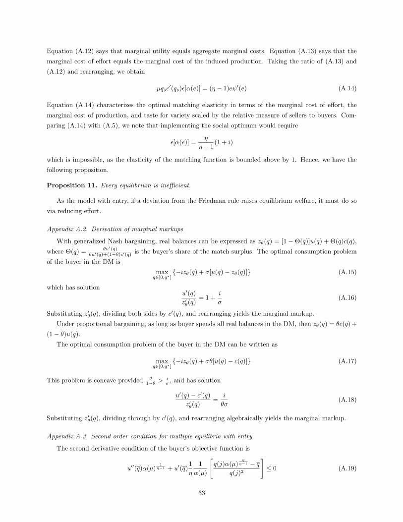
Equation (A.12) says that marginal utility equals aggregate marginal costs. Equation (A.13) says that the

marginal cost of effort equals the marginal cost of the induced production. Taking the ratio of (A.13) and

(A.12) and rearranging, we obtain

µqsc′(qs)ε[α(e)] = (η − 1)eψ′(e) (A.14)

Equation (A.14) characterizes the optimal matching elasticity in terms of the marginal cost of effort, the

marginal cost of production, and taste for variety scaled by the relative measure of sellers to buyers. Com-

paring (A.14) with (A.5), we note that implementing the social optimum would require

ε[α(e)] =η

η − 1(1 + i)

which is impossible, as the elasticity of the matching function is bounded above by 1. Hence, we have the

following proposition.

Proposition 11. Every equilibrium is inefficient.

As the model with entry, if a deviation from the Friedman rule raises equilibrium welfare, it must do so

via reducing effort.

Appendix A.2. Derivation of marginal markups

With generalized Nash bargaining, real balances can be expressed as zθ(q) = [1 − Θ(q)]u(q) + Θ(q)c(q),

where Θ(q) = θu′(q)θu′(q)+(1−θ)c′(q) is the buyer’s share of the match surplus. The optimal consumption problem

of the buyer in the DM is

maxq∈[0,q∗]

−izθ(q) + σ[u(q)− zθ(q)] (A.15)

which has solutionu′(q)

z′θ(q)= 1 +

i

σ(A.16)

Substituting z′θ(q), dividing both sides by c′(q), and rearranging yields the marginal markup.

Under proportional bargaining, as long as buyer spends all real balances in the DM, then zθ(q) = θc(q) +

(1− θ)u(q).

The optimal consumption problem of the buyer in the DM can be written as

maxq∈[0,q∗]

−izθ(q) + σθ[u(q)− c(q)] (A.17)

This problem is concave provided θ1−θ >

iσ , and has solution

u′(q)− c′(q)z′θ(q)

=i

θσ(A.18)

Substituting z′θ(q), dividing through by c′(q), and rearranging algebraically yields the marginal markup.

Appendix A.3. Second order condition for multiple equilibria with entry

The second derivative condition of the buyer’s objective function is

u′′(q)α(µ)1

η−1 + u′(q)1

η

1

α(µ)

[q(j)α(µ)

ηη−1 − q

q(j)2

]≤ 0 (A.19)

33

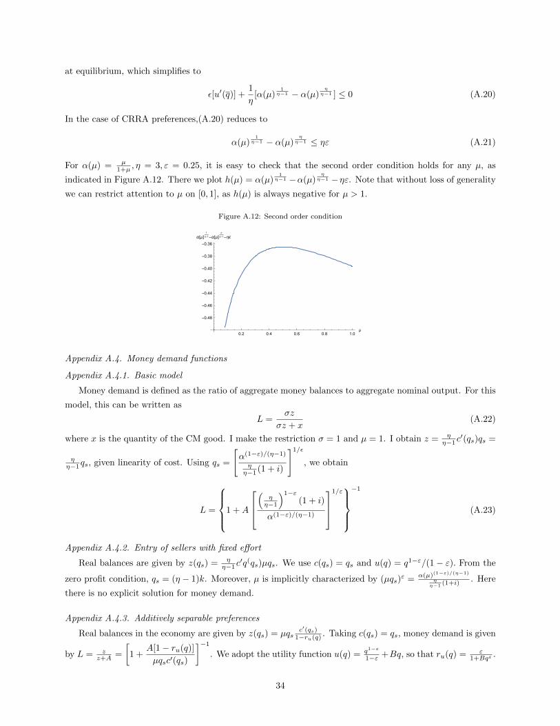
at equilibrium, which simplifies to

ε[u′(q)] +1

η[α(µ)

1η−1 − α(µ)

ηη−1 ] ≤ 0 (A.20)

In the case of CRRA preferences,(A.20) reduces to

α(µ)1

η−1 − α(µ)ηη−1 ≤ ηε (A.21)

For α(µ) = µ1+µ , η = 3, ε = 0.25, it is easy to check that the second order condition holds for any µ, as

indicated in Figure A.12. There we plot h(µ) = α(µ)1

η−1 −α(µ)ηη−1 −ηε. Note that without loss of generality

we can restrict attention to µ on [0, 1], as h(µ) is always negative for µ > 1.

Figure A.12: Second order condition

0.2 0.4 0.6 0.8 1.0μ

-0.48

-0.46

-0.44

-0.42

-0.40

-0.38

-0.36

α[μ]1

η-1-α[μ]η

η-1-ηϵ

Appendix A.4. Money demand functions

Appendix A.4.1. Basic model

Money demand is defined as the ratio of aggregate money balances to aggregate nominal output. For this

model, this can be written as

L =σz

σz + x(A.22)

where x is the quantity of the CM good. I make the restriction σ = 1 and µ = 1. I obtain z = ηη−1c

′(qs)qs =

ηη−1qs, given linearity of cost. Using qs =

[α(1−ε)/(η−1)

ηη−1 (1 + i)

]1/ε

, we obtain

L =

1 +A

(

ηη−1

)1−ε(1 + i)

α(1−ε)/(η−1)

1/ε−1

(A.23)

Appendix A.4.2. Entry of sellers with fixed effort

Real balances are given by z(qs) = ηη−1c

′q(qs)µqs. We use c(qs) = qs and u(q) = q1−ε/(1− ε). From the

zero profit condition, qs = (η − 1)k. Moreover, µ is implicitly characterized by (µqs)ε = α(µ)(1−ε)/(η−1)

ηη−1 (1+i) . Here

there is no explicit solution for money demand.

Appendix A.4.3. Additively separable preferences

Real balances in the economy are given by z(qs) = µqsc′(qs)

1−ru(q) . Taking c(qs) = qs, money demand is given

by L = zz+A =

[1 +

A[1− ru(q)]

µqsc′(qs)

]−1

. We adopt the utility function u(q) = q1−ε

1−ε +Bq, so that ru(q) = ε1+Bqε .

34

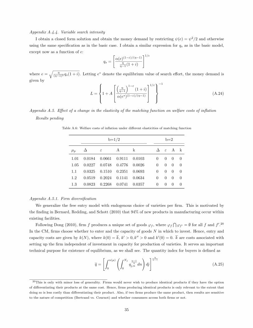
Appendix A.4.4. Variable search intensity

I obtain a closed form solution and obtain the money demand by restricting ψ(e) = ψ2/2 and otherwise

using the same specification as in the basic case. I obtain a similar expression for qs as in the basic model,

except now as a function of e:

qs =

[α(e)(1−ε)/(η−1)

ηη−1 (1 + i)

]1/ε

where e =√

η(η−1)2 qs(1 + i). Letting e∗ denote the equilibrium value of search effort, the money demand is

given by

L =

1 +A

(

ηη−1

)1−ε(1 + i)

α(e∗)(1−ε)/(η−1)

1/ε−1

(A.24)

Appendix A.5. Effect of a change in the elasticity of the matching function on welfare costs of inflation

Results pending

Table A.6: Welfare costs of inflation under different elasticities of matching function

b=1/2 b=2

µp ∆ ε A k ∆ ε A k

1.01 0.0184 0.0661 0.9111 0.0103 0 0 0 0

1.05 0.0227 0.0748 0.4776 0.0026 0 0 0 0

1.1 0.0325 0.1510 0.2351 0.0693 0 0 0 0

1.2 0.0519 0.2024 0.1141 0.0634 0 0 0 0

1.3 0.0823 0.2268 0.0741 0.0357 0 0 0 0

Appendix A.5.1. Firm diversification

We generalize the free entry model with endogenous choice of varieties per firm. This is motivated by

the finding in Bernard, Redding, and Schott (2010) that 94% of new products in manufacturing occur within

existing facilities.

Following Dong (2010), firm f produces a unique set of goods ϕf , where ϕf⋂ϕf ′ = ∅ for all f and f ′.20

In the CM, firms choose whether to enter and the capacity of goods N in which to invest. Hence, entry and

capacity costs are given by k(N), where k(0) = k, k′ > 0, k′′ > 0 and k′(0) = 0. k are costs associated with

setting up the firm independent of investment in capacity for production of varieties. It serves an important

technical purpose for existence of equilibrium, as we shall see. The quantity index for buyers is defined as

q =

[∫ α(µ)

0

(∫ Nj

0

qη−1η

j,n dn

)dj

] ηη−1

(A.25)

20This is only with minor loss of generality. Firms would never wish to produce identical products if they have the option

of differentiating their products at the same cost. Hence, firms producing identical products is only relevant to the extent that

doing so is less costly than differentiating their product. Also, if two firms produce the same product, then results are sensitive

to the nature of competition (Bertrand vs. Cournot) and whether consumers access both firms or not.

35

where qj,n is the quantity of variety n offered by firm j. The problem of the buyer yields

(1 + i)pj,n = [Nα(µ)]1

η−1u′(q)

(q

qj,n

) 1η

(A.26)

Anticipating product symmetry, let q = qn,j for all n, j, so that q = [Nα(µ)]ηη−1 q and the quantity of each

variety is given by qs = α(µ)µ q. This implies q = [Nα(µ)]

1η−1µNqs. q thus consists of total production µNqs

scaled according to the number of varieties each consumer accesses and the taste for variety [Nα(µ)]1

η−1 .

The marginal markup in equilibrium is given by

u′[(Nα(µ))1

η−1µNqs]

c′(qs)=

η

η − 1(1 + i) (A.27)

The maximization problem over the number of varieties is given by

maxN

−k(N) +N

[η

η − 1c′(qs)qs − c(qs)

](A.28)

where qs = αsq, given the inverse demand of the buyer qj . Given the assumptions on k(·), there is an interior

solution given by

k′(N) =η

η − 1c′(qs)qs − c(qs) (A.29)

The firm equates the marginal cost of a new production line with the profits of the associated variety. In

contrast to Dong, the benefit consists of selling greater varieties to the same set of customers rather than

increasing the probability of supplying consumers’ desired variety.

Firm size is given by Nqs, the measure of varieties multiplied by the quantity of each variety. The free

entry condition, in turn, is characterized by

k(N) +Nc(qs) = Nη

η − 1c′(qs)qs (A.30)

Noting that average costs are given by k(N)+Nc(qs)Nqs

, so that the ratio of average to marginal costs is given byk(N)N +c(qs)

qsc′(qs)= η

η−1 , which is the standard free entry condition with k(N)/N in place of k.

Note that (A.29) and (A.30) can be combined to yield

k′(N) =k(N)

N(A.31)

This result is a consequence of free entry, and is independent of CES. In particular, firm entry drives average

costs of investment in capacity to its minimum, which occurs at k′(N) = k(N)N , or εk(N) = 1. Since k(·)

is convex, a solution to (A.31) requires k > 0. Note that, with Ne determined from (A.31), qs can be

determined from (A.30) and µ can be determined from (A.27). Hence, equilibrium is a triple (N, qs, µ)

that satisfies (A.31), (A.30), and (A.30). Due to the recursive structure, the conditions for existence and

uniqueness are identical to the free entry equilibrium. Analogously to the free entry model, define λ(µ) =

[Neα(µ)]1

η−1u′[(Neα(µ))1

η−1µNeqes ], which is marginal utility as a function of the sellers, given N = Ne and

qs = qes .

From the recursive structure of equilibrium, N and qs do not depend on i. A higher nominal interest

rate shifts the cost of holding real balances higher, and through (A.27) reduces the entry of sellers, provided

λ′(µ) < 0. Hence, inflation reduces variety only by affecting the entry of sellers, not by reducing the varieties

of each firm. It is easy to see that in the absence of free entry, however, inflation would reduce the varieties

36

offered by each firm. This arises from the basic model, in which qs decreases inflation. Here, N would be

decreasing with qs and, hence, with inflation. Thus, with a fixed measure of sellers, we recover the result in

Dong that both quantity and variety decrease with inflation.

This generalization provides an account of the tradeoff between firm diversification vs. specialization.

Producing more varieties allows a firm to extract additional profits given by ηη−1c

′(qs)qs − c(qs), but faces

convex costs of investment in capacity.

37

Arkolakis, C., Costinot, A., Donaldson, D., Rodrıguez-Clare, A., 2012. The elusive pro-competitive effects of

trade. Unpublished, MIT.

Aruoba, S. B., Schorfheide, F., 2011. Sticky prices versus monetary frictions: An estimation of policy trade-

offs. American Economic Journal: Macroeconomics 3 (1), 60–90.

Bilbiie, F., Ghironi, F., Melitz, M. J., Nov. 2007. Endogenous Entry, Product Variety, and Business Cycles.

NBER Working Papers 13646, National Bureau of Economic Research, Inc.

URL http://ideas.repec.org/p/nbr/nberwo/13646.html

Craig, B., Rocheteau, G., 2008. Inflation and welfare: A search approach. Journal of Money, Credit and

Banking 40 (1), 89–119.

Dixit, A. K., Stiglitz, J. E., 1977. Monopolistic competition and optimum product diversity. The American

Economic Review, 297–308.

Dong, M., 2010. Inflation and variety*. International Economic Review 51 (2), 401–420.

Faig, M., Jerez, B., 2006. Inflation, prices, and information in competitive search. Advances in Macroeco-

nomics 6 (1), 1–34.

Galenianos, M., Kircher, P., 2008. A model of money with multilateral matching. Journal of Monetary

Economics 55 (6), 1054–1066.

Galı, J., 2009. Monetary Policy, inflation, and the Business Cycle: An introduction to the new Keynesian

Framework. Princeton University Press.

Hosios, A. J., 1990. On the efficiency of matching and related models of search and unemployment. The

Review of Economic Studies 57 (2), 279–298.

Kocherlakota, N. R., 2005. Optimal monetary policy: What we know and what we don’t know*. International

Economic Review 46 (2), 715–729.

Krugman, P., June 1991. Increasing returns and economic geography. Journal of Political Economy 99 (3),

483–99.

URL http://ideas.repec.org/a/ucp/jpolec/v99y1991i3p483-99.html

Krugman, P. R., 1979. Increasing returns, monopolistic competition, and international trade. Journal of

international Economics 9 (4), 469–479.

Lagos, R., Rocheteau, G., 2005. Inflation, output, and welfare*. International Economic Review 46 (2),

495–522.

Lucas Jr, R. E., 2000. Inflation and welfare. Econometrica 68 (2), 247–274.

Melitz, M. J., Ottaviano, G. I., 2008. Market size, trade, and productivity. The review of economic studies

75 (1), 295–316.

Nosal, E., Rocheteau, G., 2011. Money, payments, and liquidity. MIT press.

38

Ottaviano, G. I., Tabuchi, T., Thisse, J.-F., 2002. Agglomeration and trade revisited. International Economic

Review 43, 409–436.

Pissarides, C. A., 1990. Equilibrium unemployment theory. MIT press.

Rocheteau, G., Wright, R., 2005. Money in search equilibrium, in competitive equilibrium, and in competitive

search equilibrium. Econometrica 73 (1), 175–202.

Romer, P. M., 1990. Endogenous technological change. Journal of political Economy, S71–S102.

Zhelobodko, E., Kokovin, S., Parenti, M., Thisse, J.-F., 2012. Monopolistic competition: Beyond the constant

elasticity of substitution. Econometrica 80 (6), 2765–2784.

39