SEARCH FOR POINT-LIKE SOURCES OF COSMIC RAYS WITH ENERGIES ABOVE

1018.5 eV IN THE HIRES–I MONOCULAR DATASET

by

Malina Aurelia Kirn

A thesis submitted in partial fulfillmentof the requirements for the degree

of

Master of Science

in

Physics

MONTANA STATE UNIVERSITYBozeman, Montana

April 2005

c© COPYRIGHT

by

Malina Aurelia Kirn

2005

All Rights Reserved

ii

APPROVAL

of a thesis submitted by

Malina Aurelia Kirn

This thesis has been read by each member of the thesis committee and has been foundto be satisfactory regarding content, English usage, format, citations, bibliographic style, andconsistency, and is ready for submission to the College of Graduate Studies.

Dr. William Hiscock

Approved for the Department of Physics

Dr. William Hiscock

Approved for the College of Graduate Studies

Dr. Bruce McLeod

iii

STATEMENT OF PERMISSION TO USE

In presenting this thesis in partial fulfillment of the requirements for a master’s degree at

Montana State University, I agree that the Library shall make it available to borrowers under

rules of the Library.

If I have indicated my intention to copyright this thesis by including a copyright notice

page, copying is allowable only for scholarly purposes, consistent with “fair use” as prescribed

in the U.S. Copyright Law. Only the copyright holder may grant requests for permission for

extended quotation from or reproduction of this thesis in whole or in parts.

Malina Aurelia Kirn

April 1, 2005

iv

ACKNOWLEDGMENTS

This work is supported by US NSF grants PHY-9321949 PHY-9974537, PHY-9904048,

PHYS-0245428, PHY-0140688, by the DOE grant FG03-92ER40732, and by the Australian

Research Council. M.A.K. thanks the Montana Space Grant Consortium for support through

a fellowship. We gratefully acknowledge the contributions from the technical staffs of our

home institutions and the Utah Center for High Performance Computing. The cooperation

of Colonels E. Fischer and G. Harter, the US Army, and the Dugway Proving Ground staff is

greatly appreciated.

v

TABLE OF CONTENTS

1. INTRODUCTION . . . . . . . . . . . . . . . . . . . . . . . . . . . . . . . . . . . . 1Ultra-High Energy Cosmic Rays . . . . . . . . . . . . . . . . . . . . . . . . . . . . . 1Previous Spectrum and Composition Results . . . . . . . . . . . . . . . . . . . . . . 1Previous Anisotropy Searches . . . . . . . . . . . . . . . . . . . . . . . . . . . . . . 4

2. THE HIGH–RESOLUTION FLY’S EYE . . . . . . . . . . . . . . . . . . . . . . . . 6The HiRes Spectrum . . . . . . . . . . . . . . . . . . . . . . . . . . . . . . . . . . . 7HiRes Anisotropy Searches . . . . . . . . . . . . . . . . . . . . . . . . . . . . . . . . 9

Global Dipole Enhancements . . . . . . . . . . . . . . . . . . . . . . . . . . . . 9Overlap With AGASA Clusters . . . . . . . . . . . . . . . . . . . . . . . . . . 11Autocorrelation Studies . . . . . . . . . . . . . . . . . . . . . . . . . . . . . . 13

Summary: Goals of This Thesis . . . . . . . . . . . . . . . . . . . . . . . . . . . . . 15

3. THE HIRES MONOCULAR DATASET . . . . . . . . . . . . . . . . . . . . . . . . 16Airshower Reconstruction . . . . . . . . . . . . . . . . . . . . . . . . . . . . . . . . 16Density Skymaps . . . . . . . . . . . . . . . . . . . . . . . . . . . . . . . . . . . . . 19

4. ISOTROPIC BACKGROUND, COMPARISON TO REAL DATA, SIMULATIONOF POINT–LIKE SOURCES . . . . . . . . . . . . . . . . . . . . . . . . . . . . . . 23The Monte Carlo Generated Isotropic Background . . . . . . . . . . . . . . . . . . . 23Isotropic Background Corrected Skymaps . . . . . . . . . . . . . . . . . . . . . . . . 25Monte Carlo Simulation of Point–Like Sources . . . . . . . . . . . . . . . . . . . . . 26

5. CRITERIA FOR DECLARATION OF A POINT SOURCE . . . . . . . . . . . . . 31

6. SENSITIVITY, UPPER LIMITS . . . . . . . . . . . . . . . . . . . . . . . . . . . . 35Sensitivity . . . . . . . . . . . . . . . . . . . . . . . . . . . . . . . . . . . . . . . . . 36Upper Limits . . . . . . . . . . . . . . . . . . . . . . . . . . . . . . . . . . . . . . . 36

7. CONCLUSIONS . . . . . . . . . . . . . . . . . . . . . . . . . . . . . . . . . . . . . 39Additional Capabilities of this Analysis Technique . . . . . . . . . . . . . . . . . . . 39

Search for Pointlike Excess in a Small Region . . . . . . . . . . . . . . . . . . 39Search for Small Extended Sources . . . . . . . . . . . . . . . . . . . . . . . . 40Including Charged Particles from Point Sources . . . . . . . . . . . . . . . . . 40

The Future of UHECR Studies . . . . . . . . . . . . . . . . . . . . . . . . . . . . . 41

REFERENCES CITED . . . . . . . . . . . . . . . . . . . . . . . . . . . . . . . . . . . 44

vi

LIST OF TABLES

Table Page

6.1 Declination, right ascension, N.33, N.15, exposure, sensitivity, and flux upperlimit at each grid point . . . . . . . . . . . . . . . . . . . . . . . . . . . . . . . 38

vii

LIST OF FIGURES

Figure Page

1.1 An example shower of secondary particles due to an incident UHECR. . . . . . 1

1.2 The energy spectrum of cosmic rays. . . . . . . . . . . . . . . . . . . . . . . . 3

1.3 Energy vs. propagation distance of several high energy protons shows rapid lossof energy due to collisions with the CMB. . . . . . . . . . . . . . . . . . . . . 3

1.4 Shower penetration depth into atmosphere vs. energy. . . . . . . . . . . . . . . 4

1.5 Cygnus X-3 in x-rays as observed by CHANDRA. . . . . . . . . . . . . . . . . 5

2.1 The HiRes–II detector before installation of the photomultiplier tube arrays. . 6

2.2 A single detector: a mirror and array of photomultiplier tubes. . . . . . . . . . 6

2.3 The “Fly’s Eye,” the grid of photomultiplier tubes used to detect nitrogenfluorescence. . . . . . . . . . . . . . . . . . . . . . . . . . . . . . . . . . . . . . 7

2.4 A cosmic ray shower as seen by the HiRes–I detector. . . . . . . . . . . . . . . 7

2.5 Plot of E3 times the flux of cosmic rays versus energy for AGASA, HiRes–I andHiRes–II monocular data. . . . . . . . . . . . . . . . . . . . . . . . . . . . . . 8

2.6 Plot of E3 times the flux of cosmic rays versus energy for the Fly’s Eye stereo [4],HiRes–I and HiRes–II monocular energy spectrums. . . . . . . . . . . . . . . . 8

2.7 Angular separation of HiRes–I monocular data from the galactic center. . . . . 10

2.8 Angular separation from the galactic center expected from an isotropic distri-bution. . . . . . . . . . . . . . . . . . . . . . . . . . . . . . . . . . . . . . . . . 10

2.9 Background corrected angular separation of HiRes–I monocular data from thegalactic center. . . . . . . . . . . . . . . . . . . . . . . . . . . . . . . . . . . . 10

2.10 Number of overlaps with AGASA clusters for HiRes–I events with energy greaterthan 4 x 1019 eV. . . . . . . . . . . . . . . . . . . . . . . . . . . . . . . . . . . 12

2.11 Number of overlaps with AGASA clusters for HiRes–I events with energy greaterthan 2.65 x 1019 eV. . . . . . . . . . . . . . . . . . . . . . . . . . . . . . . . . 12

2.12 Arrival directions of HiRes–I monocular events and their “error ellipses” (seeChapter 3) with energy greater than 2.65 x 1019 eV shown with AGASA clusters. 12

2.13 Autocorrelation observed in HiRes–I monocular data. . . . . . . . . . . . . . . 14

viii

2.14 Autocorrelation observed in AGASA data. . . . . . . . . . . . . . . . . . . . . 14

2.15 Autocorrelation observed in HiRes stereo data. . . . . . . . . . . . . . . . . . . 14

3.1 The central coordinates of events in the HiRes–I monocular data set: 1,525events with energies exceeding 1018.5 eV. . . . . . . . . . . . . . . . . . . . . . 17

3.2 Diagrams of event reconstruction. . . . . . . . . . . . . . . . . . . . . . . . . . 18

3.3 The energies of events reconstructed using monocular and stereo techniquesseparately. . . . . . . . . . . . . . . . . . . . . . . . . . . . . . . . . . . . . . . 19

3.4 Comparison of HiRes–I data (points) and Monte Carlo (solid histogram) distri-butions in zenith angles (degrees). . . . . . . . . . . . . . . . . . . . . . . . . . 20

3.5 Comparison of HiRes–I data (points) and Monte Carlo (solid histogram) distri-butions in distance to shower core (km). . . . . . . . . . . . . . . . . . . . . . 20

3.6 The geometry of reconstruction for a monocular air fluorescence detector. . . . 20

3.7 Distribution of σSDP for the HiRes–I monocular data set . . . . . . . . . . . . 21

3.8 Distribution of σΨ for the HiRes–I monocular data set . . . . . . . . . . . . . . 21

3.9 “Error ellipses” of a few sample points. . . . . . . . . . . . . . . . . . . . . . . 21

3.10 Skymap of arrival directions of events in the the HiRes–I monocular dataset,plotted in polar projection, equatorial coordinates. . . . . . . . . . . . . . . . . 22

4.1 Comparison of HiRes–I data (points) and Monte Carlo (solid histogram) distri-butions in right ascension (RA). . . . . . . . . . . . . . . . . . . . . . . . . . . 24

4.2 Comparison of HiRes–I data (points) and Monte Carlo (solid histogram) distri-butions in declination (DEC). . . . . . . . . . . . . . . . . . . . . . . . . . . . 24

4.3 σMC (Equation 4.2) distribution, the standard deviation of the Monte Carlo bindensity. . . . . . . . . . . . . . . . . . . . . . . . . . . . . . . . . . . . . . . . 25

4.4 〈NMC〉 distribution graphically demonstrates the effects of summer/winter nightson our exposure. . . . . . . . . . . . . . . . . . . . . . . . . . . . . . . . . . . 25

4.5 χ1 distribution for the HiRes-I monocular data set . . . . . . . . . . . . . . . . 26

4.6 Example distribution of χ1 values for 1,000 MC data sets in the bin located at5 hours RA, 40◦ DEC. . . . . . . . . . . . . . . . . . . . . . . . . . . . . . . . 27

4.7 Skymap of example source without an isotropic background. . . . . . . . . . . 28

ix

4.8 Skymap of arrival directions of events for a Monte Carlo dataset, having thesame overall exposure as the HiRes–I monocular dataset, with a 25 event sourcesuperimposed at 5 hours RA, 40◦ DEC. . . . . . . . . . . . . . . . . . . . . . . 29

4.9 χ1 for NS = 25 event source inserted in a simulated isotropic dataset. . . . . . 30

5.1 F distribution derived from the χ1 map of the example source shown in Figure 4.9. 32

5.2 Occurrence rate of false positives versus F for a 2.5◦ search circle and χ1 thresh-old of 4. . . . . . . . . . . . . . . . . . . . . . . . . . . . . . . . . . . . . . . . 33

5.3 F distribution for the HiRes–I monocular data. . . . . . . . . . . . . . . . . . 34

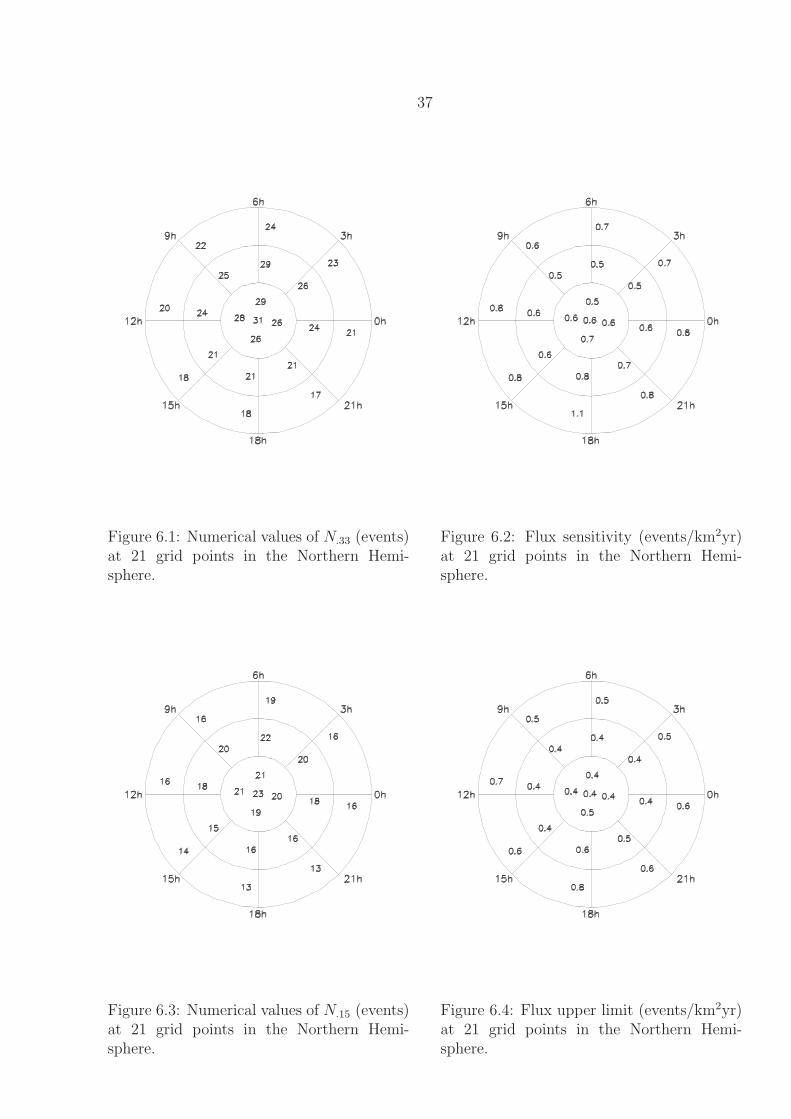
6.1 Numerical values of N.33 (events) at 21 grid points in the Northern Hemisphere. 37

6.2 Flux sensitivity (events/km2yr) at 21 grid points in the Northern Hemisphere. 37

6.3 Numerical values of N.15 (events) at 21 grid points in the Northern Hemisphere. 37

6.4 Flux upper limit (events/km2yr) at 21 grid points in the Northern Hemisphere. 37

7.1 Map of the Pierre Auger Observatory, a hybrid detector in the southern hemi-sphere (Argentina). . . . . . . . . . . . . . . . . . . . . . . . . . . . . . . . . . 42

7.2 Map of the Telescope Array, a proposed hybrid detector. . . . . . . . . . . . . 43

x

ABSTRACT

We report the results of a search for pointlike deviations from isotropy in the arrivaldirections of ultra–high energy cosmic rays in the northern hemisphere, carried out using askymap technique. In the monocular dataset collected by the High–Resolution Fly’s Eye,consisting of 1,525 events with energy exceeding 1018.5 eV, we find no evidence for pointlikeexcesses.

Pointlike excesses at these energies can arise from only a limited number of source scenarios.Galactic and extragalactic magnetic fields are expected to produce large perturbations in thearrival directions of charged particles. A compact arrival direction excess at these energieswould therefore suggest neutral primaries. Neutrons, however, possess a finite lifetime, thusany source of neutrons would have to be located within the Milky Way Galaxy. Results ofstudies of pointlike behavior in arrival direction of UHECR are ambiguous. While pointlikeexcesses have been observed by other experiments, previous studies of HiRes data have yieldednull results and HiRes events do not support evidence for previously identified clusters.

Our technique allows calculation of sensitivity and upper limits using Monte Carlo simu-lated sources. We place an upper limit of 0.8 events/(km2 yr) (90% c.l.) on the flux from suchsources, place more stringent upper limits as a function of position, and determine detectorsensitivity as a function of position in the sky. We also consider the historically significantsource candidate Cygnus X-3, an x-ray binary, as the focus of an a priori search and place anupper limit of 0.5 events/(km2 yr) (90% c.l.) from the direction of Cygnus X-3.

1

CHAPTER 1

INTRODUCTION

Ultra-High Energy Cosmic Rays

Ultra-High Energy Cosmic Rays (UHECR) are cosmic rays with energies exceeding roughly

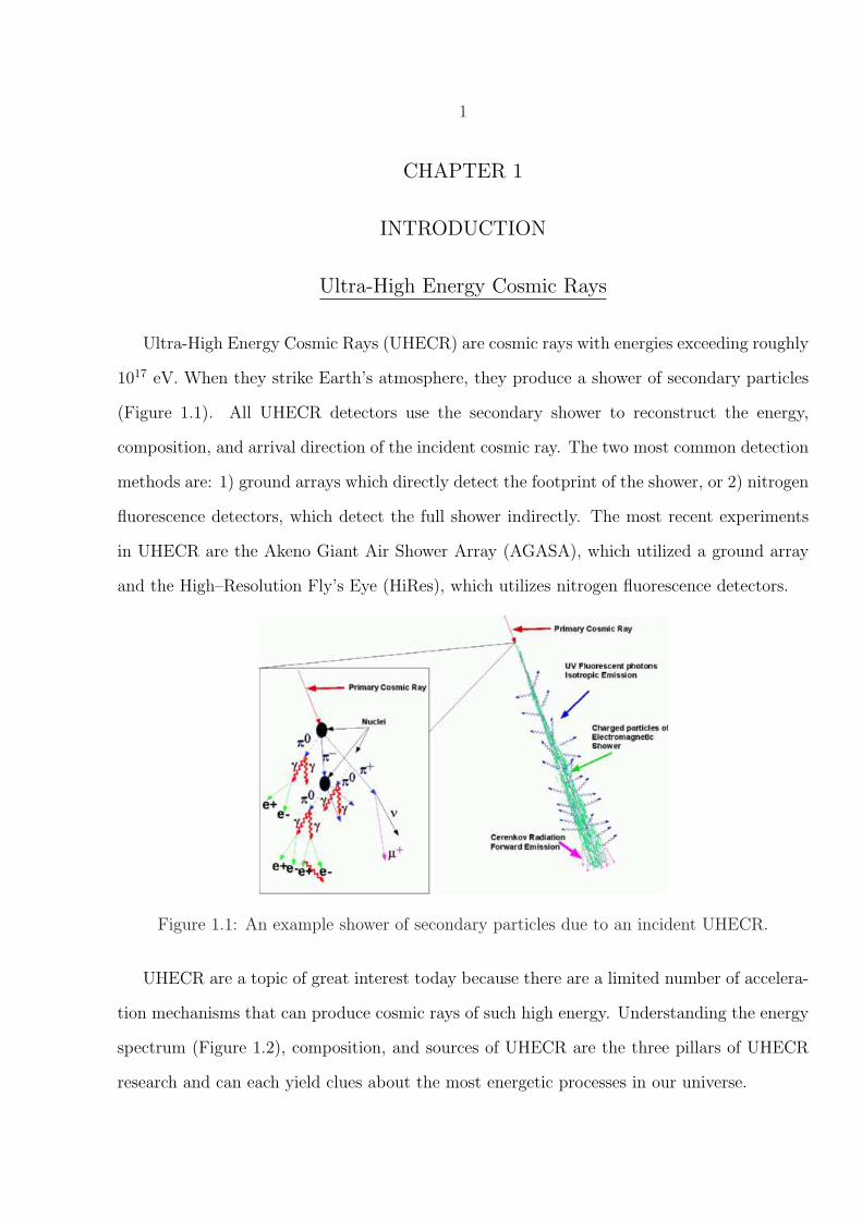
1017 eV. When they strike Earth’s atmosphere, they produce a shower of secondary particles

(Figure 1.1). All UHECR detectors use the secondary shower to reconstruct the energy,

composition, and arrival direction of the incident cosmic ray. The two most common detection

methods are: 1) ground arrays which directly detect the footprint of the shower, or 2) nitrogen

fluorescence detectors, which detect the full shower indirectly. The most recent experiments

in UHECR are the Akeno Giant Air Shower Array (AGASA), which utilized a ground array

and the High–Resolution Fly’s Eye (HiRes), which utilizes nitrogen fluorescence detectors.

Figure 1.1: An example shower of secondary particles due to an incident UHECR.

UHECR are a topic of great interest today because there are a limited number of accelera-

tion mechanisms that can produce cosmic rays of such high energy. Understanding the energy

spectrum (Figure 1.2), composition, and sources of UHECR are the three pillars of UHECR

research and can each yield clues about the most energetic processes in our universe.

2

Previous Spectrum and Composition Results

A topic of great debate in the energy spectrum of UHECR is the GZK cutoff (named for

Greisen, Zatsepin, and Kuzmin), near 6 x 1019 eV [1, 2]. Several experiments leading up to

and including AGASA indicated that the flux of UHECR may be higher than predicted by the

GZK cutoff. As UHECR propagate through the universe, they encounter radiation left from

the Big Bang, known as the Cosmic Microwave Background Radiation (CMB). Ordinarily,

cosmic rays interact infrequently with the CMB, but at these ultra-high energies, relativistic

effects due to blue-shift are a significant contributor to the rate of interaction. UHECR are

expected to dissipate their energy within a fairly short distance due to collisions with the

CMB, as seen in Figure 1.3. The primary interaction is:

p + γ2.7K → ∆+ → p + π0 , n + π+ (1.1)

and is frequently referred to as the pion production threshold. UHECR protons are expected to

dissipate their energy to below the GZK feature within order 100 Mpc and UHECR iron nuclei

within order 10 Mpc (the Milky Way galaxy is roughly 30 kpc in diameter and the nearest

large galaxy, Andromeda, is roughly .9 Mpc away). There are not many highly energetic

astrophysical objects within this distance, so a sharp reduction in the flux of cosmic rays

is expected near 6 x 1019 eV with a “pile-up” of lower energy events just prior to the drop

from events that have lost their super-GZK energies in collisions. A feature near 4 x 1018 eV,

known as the “ankle”, shows a slight change in the slope of flux vs energy (Figure 1.2) and

has been well-measured by numerous experiments [3, 4, 5, 6]. The “ankle” is similar to the

GZK feature, but is due to the electron pair production threshold (at 6 x 1017 eV) instead of

pion production. Finally, the cause of a smaller feature near 3 x 1017 eV, the “second knee,”

is not known, but may be due to the distribution of extragalactic sources or to a change in

the galactic spectrum.

3

Figure 1.2: The energy spectrum of cosmic rays.

Figure 1.3: Energy vs. propagation distance of several high energy protons shows rapid lossof energy due to collisions with the CMB.

4

UHECR are thought to be primarily protons or nuclei because acceleration mechanisms

for neutral or less massive particles do not easily yield these energy scales. Particles with

higher energy penetrate further into our atmosphere, so profiles of shower depth vs. energy

can yield clues to the composition of the incident cosmic ray. Figure 1.4 indicates there may

be a composition change from heavy to light incident cosmic rays near 1018 eV because of the

change in slope.

Figure 1.4: Shower penetration depth into atmosphere vs. energy. The slope change near1018eV is perhaps indicative of a composition change from heavy to light incident cosmic rays.

Previous Anisotropy Searches

In the search for UHECR, a variety of strategies have been employed to detect deviations

from isotropy in event arrival directions. The results of these searches have been ambiguous.

AGASA found evidence for a dipole moment in Right Ascension (RA) at energies above 1018

eV [7]. They attribute the dipole moment to an excess either from the galactic center or Cygnus

X-3, an x-ray binary within our galaxy (Figure 1.5). On smaller angular scales, excesses have

been alternately claimed and refuted in the vicinity of Cygnus X-3 [8, 9, 10, 11], including the

5

report of a possible excess in a point-source search [12]. AGASA also reports six point-like

clusters in their most recent published data set [13, 14, 15], including a cluster with three

events known as the “AGASA Triplet.”

Figure 1.5: Cygnus X-3 in x-rays as observed by CHANDRA. This picture is of size 200” x200” (arcseconds).

6

CHAPTER 2

THE HIGH–RESOLUTION FLY’S EYE

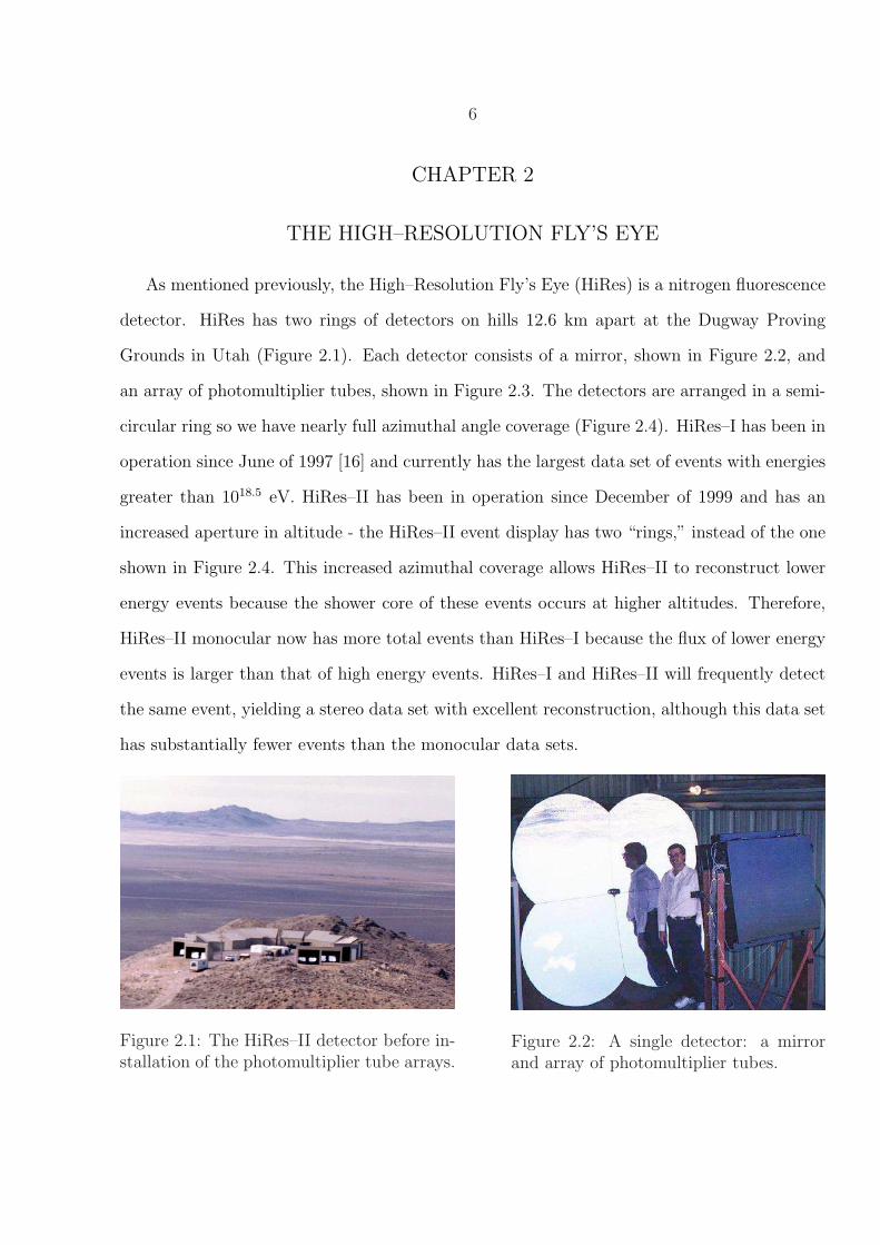
As mentioned previously, the High–Resolution Fly’s Eye (HiRes) is a nitrogen fluorescence

detector. HiRes has two rings of detectors on hills 12.6 km apart at the Dugway Proving

Grounds in Utah (Figure 2.1). Each detector consists of a mirror, shown in Figure 2.2, and

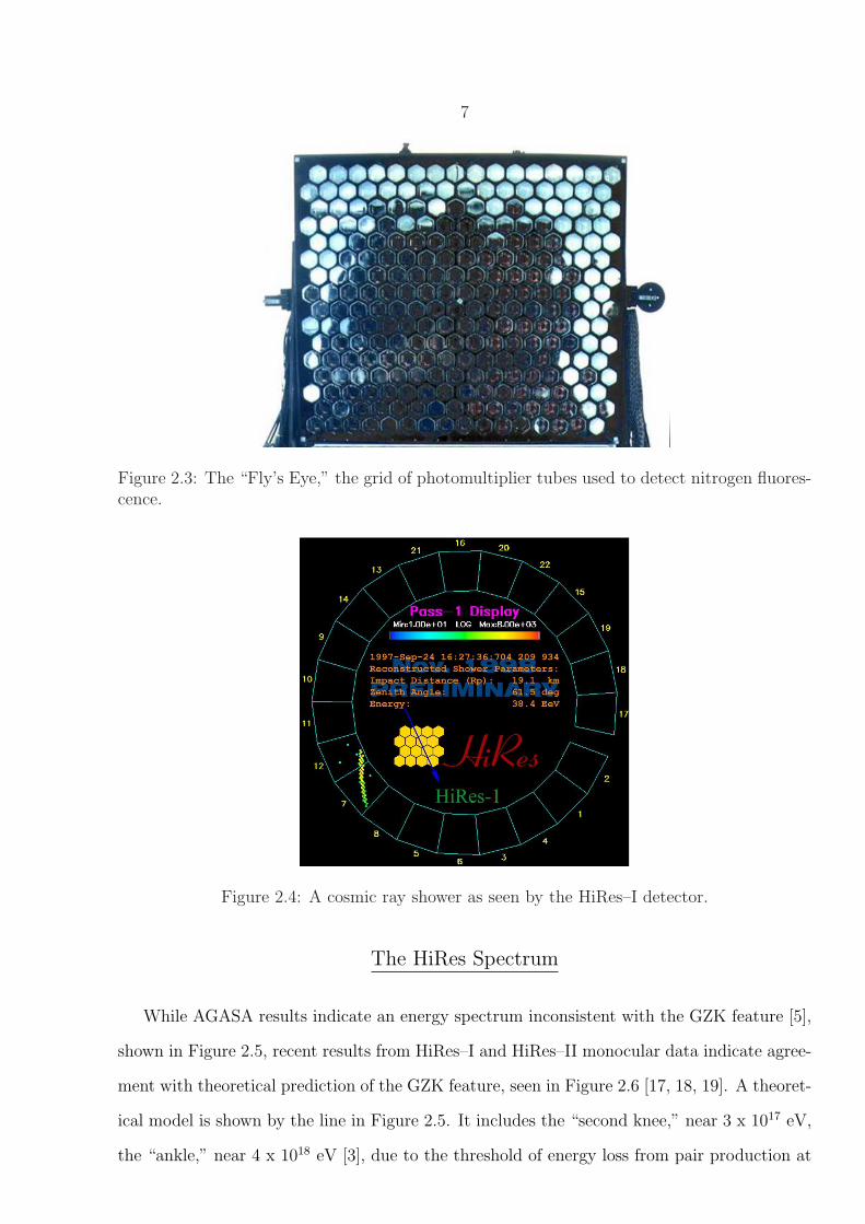
an array of photomultiplier tubes, shown in Figure 2.3. The detectors are arranged in a semi-

circular ring so we have nearly full azimuthal angle coverage (Figure 2.4). HiRes–I has been in

operation since June of 1997 [16] and currently has the largest data set of events with energies

greater than 1018.5 eV. HiRes–II has been in operation since December of 1999 and has an

increased aperture in altitude - the HiRes–II event display has two “rings,” instead of the one

shown in Figure 2.4. This increased azimuthal coverage allows HiRes–II to reconstruct lower

energy events because the shower core of these events occurs at higher altitudes. Therefore,

HiRes–II monocular now has more total events than HiRes–I because the flux of lower energy

events is larger than that of high energy events. HiRes–I and HiRes–II will frequently detect

the same event, yielding a stereo data set with excellent reconstruction, although this data set

has substantially fewer events than the monocular data sets.

Figure 2.1: The HiRes–II detector before in-stallation of the photomultiplier tube arrays.

Figure 2.2: A single detector: a mirrorand array of photomultiplier tubes.

7

Figure 2.3: The “Fly’s Eye,” the grid of photomultiplier tubes used to detect nitrogen fluores-cence.

Figure 2.4: A cosmic ray shower as seen by the HiRes–I detector.

The HiRes Spectrum

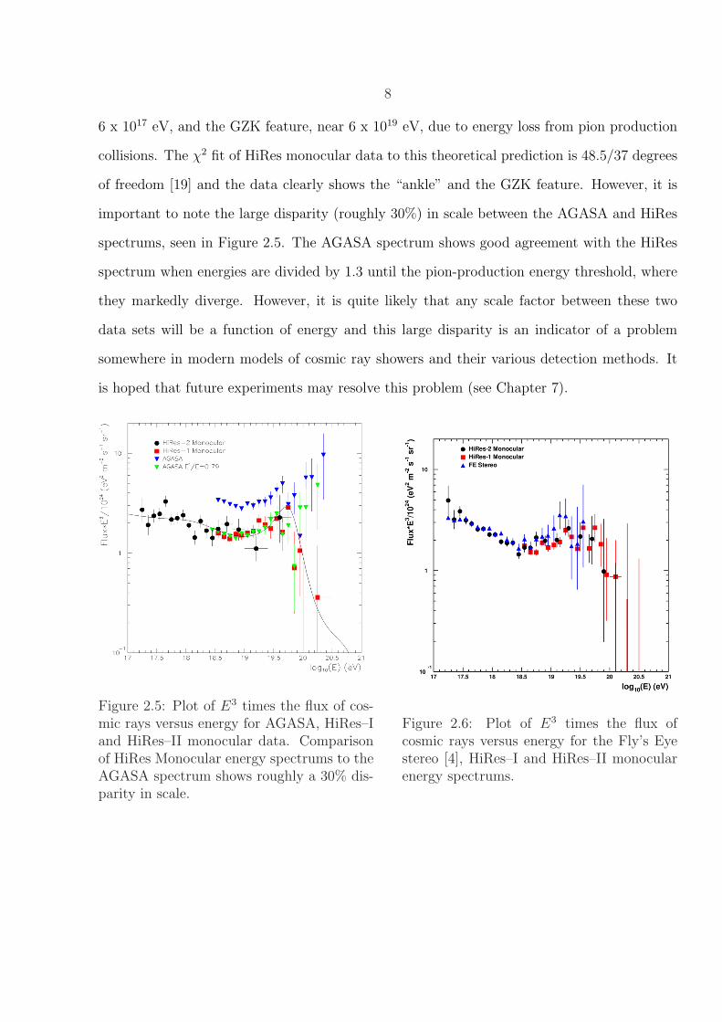
While AGASA results indicate an energy spectrum inconsistent with the GZK feature [5],

shown in Figure 2.5, recent results from HiRes–I and HiRes–II monocular data indicate agree-

ment with theoretical prediction of the GZK feature, seen in Figure 2.6 [17, 18, 19]. A theoret-

ical model is shown by the line in Figure 2.5. It includes the “second knee,” near 3 x 1017 eV,

the “ankle,” near 4 x 1018 eV [3], due to the threshold of energy loss from pair production at

8

6 x 1017 eV, and the GZK feature, near 6 x 1019 eV, due to energy loss from pion production

collisions. The χ2 fit of HiRes monocular data to this theoretical prediction is 48.5/37 degrees

of freedom [19] and the data clearly shows the “ankle” and the GZK feature. However, it is

important to note the large disparity (roughly 30%) in scale between the AGASA and HiRes

spectrums, seen in Figure 2.5. The AGASA spectrum shows good agreement with the HiRes

spectrum when energies are divided by 1.3 until the pion-production energy threshold, where

they markedly diverge. However, it is quite likely that any scale factor between these two

data sets will be a function of energy and this large disparity is an indicator of a problem

somewhere in modern models of cosmic ray showers and their various detection methods. It

is hoped that future experiments may resolve this problem (see Chapter 7).

Figure 2.5: Plot of E3 times the flux of cos-mic rays versus energy for AGASA, HiRes–Iand HiRes–II monocular data. Comparisonof HiRes Monocular energy spectrums to theAGASA spectrum shows roughly a 30% dis-parity in scale.

Figure 2.6: Plot of E3 times the flux ofcosmic rays versus energy for the Fly’s Eyestereo [4], HiRes–I and HiRes–II monocularenergy spectrums.

9

HiRes Anisotropy Searches

As of the date of publication of this thesis, HiRes has detected no pointlike or large–scale

sources in any of the monocular or stereo data sets. Discussion of a few HiRes anisotropy

searches follows.

Global Dipole Enhancements

The most recent results [20] have supported the null hypothesis for large–scale dipole

behavior in arrival directions for particles above 1018.5 eV in the HiRes–I monocular data.

Global dipole enhancements look for a surplus in half of the sky and a deficit in the opposing

half. It is useful for extended objects, such as the galactic core, or for sources with particle

trajectories that experience significant magnetic deflection. To calculate dipole moment, a

potential source is chosen and the angle between the source and each event is calculated.

Figure 2.7 shows the event distribution in cos(θ) for the HiRes–I monocular data, where θ is

the angular separation of events from the galactic center. Figure 2.8 shows the corresponding

plot for a Monte Carlo generated isotropic background and Figure 2.9 for the background

corrected data. The background corrected distribution is then fit with the function [21]:

n =1

2+

α

2cos(θ) (2.1)

where n is the number of events in each bin and α is the dipole moment, given by the fit. α = 1

corresponds to a strong dipole moment from the potential source, α = −1 to a strong dipole

moment opposite the potential source, while α = 0 corresponds to an isotropic distribution

in dipole moment from the potential source. Calculation of α yields −.010 ± .055 for the

galactic core, −.035 ± .060 for Centaurus A, and −.005 ± .045 for M87 [20]. Thus, HiRes–I

measures no global dipole enhancement from the galactic core, Centaurus A, or M87. When

the analysis is done including HiRes–I angular resolution, values of α are nearly unchanged

(see Reference [20]) and are still consistent with the null result for a global dipole enhancement

from these three candidates.

10

Figure 2.7: Angular separation of HiRes–Imonocular data from the galactic center.

Figure 2.8: Angular separation from thegalactic center expected from an isotropicdistribution.

Figure 2.9: Background corrected angular separation of HiRes–I monocular data from thegalactic center.

11

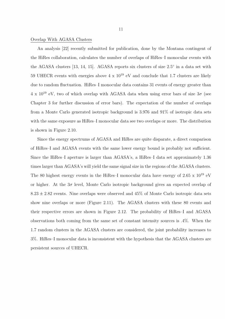
Overlap With AGASA Clusters

An analysis [22] recently submitted for publication, done by the Montana contingent of

the HiRes collaboration, calculates the number of overlaps of HiRes–I monocular events with

the AGASA clusters [13, 14, 15]. AGASA reports six clusters of size 2.5◦ in a data set with

59 UHECR events with energies above 4 x 1019 eV and conclude that 1.7 clusters are likely

due to random fluctuation. HiRes–I monocular data contains 31 events of energy greater than

4 x 1019 eV, two of which overlap with AGASA data when using error bars of size 3σ (see

Chapter 3 for further discussion of error bars). The expectation of the number of overlaps

from a Monte Carlo generated isotropic background is 3.976 and 91% of isotropic data sets

with the same exposure as HiRes–I monocular data see two overlaps or more. The distribution

is shown in Figure 2.10.

Since the energy spectrums of AGASA and HiRes are quite disparate, a direct comparison

of HiRes–I and AGASA events with the same lower energy bound is probably not sufficient.

Since the HiRes–I aperture is larger than AGASA’s, a HiRes–I data set approximately 1.36

times larger than AGASA’s will yield the same signal size in the regions of the AGASA clusters.

The 80 highest energy events in the HiRes–I monocular data have energy of 2.65 x 1019 eV

or higher. At the 3σ level, Monte Carlo isotropic background gives an expected overlap of

8.23 ± 2.82 events. Nine overlaps were observed and 45% of Monte Carlo isotropic data sets

show nine overlaps or more (Figure 2.11). The AGASA clusters with these 80 events and

their respective errors are shown in Figure 2.12. The probability of HiRes–I and AGASA

observations both coming from the same set of constant intensity sources is .4%. When the

1.7 random clusters in the AGASA clusters are considered, the joint probability increases to

3%. HiRes–I monocular data is inconsistent with the hypothesis that the AGASA clusters are

persistent sources of UHECR.

12

Figure 2.10: Number of overlaps withAGASA clusters for HiRes–I events with en-ergy greater than 4 x 1019 eV. Expectation ofthe number of overlaps from a Monte Carlogenerated isotropic background is shown asthe histogram with the actual number ob-served (2) indicated by the arrow.

Figure 2.11: Number of overlaps withAGASA clusters for HiRes–I events with en-ergy greater than 2.65 x 1019 eV. Expectationof the number of overlaps from a Monte Carlogenerated isotropic background is shown asthe histogram with the actual number ob-served (9) indicated by the arrow.

Figure 2.12: Arrival directions of HiRes–I monocular events and their “error ellipses” (seeChapter 3) with energy greater than 2.65 x 1019 eV shown with AGASA clusters. Coordinatesare shown as a polar projection of equatorial coordinates.

13

Autocorrelation Studies

The basic technique of autocorrelation is similar to that of a global dipole search except

separation angles are calculated between every pair of points instead of between a potential

source and the points. Autocorrelation provides a measure of small scale anisotropy and is

useful for determining if pointlike behavior in arrival direction exists within a data set. If

pointlike behavior exists, one would expect a peak for small angles in the distribution of

angular separation between events. A recently published paper [23] applied autocorrelation

techniques to 52 events from the HiRes–I monocular data set with energies exceeding 3 x 1019

eV and the AGASA data set. No peak was observed for HiRes–I data (Figure 2.13) while

a substantial peak for small angles was seen in AGASA data (Figure 2.14). Thus, HiRes–

I monocular data is consistent with the null hypothesis for clustering at small angles. By

simulation of doublets on a Monte Carlo generated isotropic background, it was determined

with 90% confidence that HiRes–I is sensitive to 3.5 doublets above background and no more

than 13% of HiRes–I events share common arrival directions.

Another autocorrelation study was done on stereo data from HiRes as a function of en-

ergy [24]. The analysis included 271 well-reconstructed events with energies greater than

1019 eV. The results of the analysis are shown in Figure 2.15, where the color scale gives the

probability of measuring the same number of event pairs or more with the same energy and

separation angle of each bin. The lower the probability, the more significant the autocorrela-

tion. The most significant autocorrelation measured 10 pairs of events with separation angle

2.2◦ and an energy of 1.69 x 1019 eV, where 1.9% of isotropic data sets with the same exposure

as HiRes stereo also measured 10 pairs or more with the same separation angle and energy.

However, when the same analysis was applied over many Monte Carlo generated isotropic

data sets, 52% measured the same probability of 1.9% or less somewhere in the plot shown in

Figure 2.15. Thus, HiRes stereo data is also consistent with the null hypothesis for small-scale

clustering. Additionally, when two doublets (four events) were inserted into multiple isotropic

data sets and the analysis was repeated for each one, the chance probability with 90% con-

fidence was 9%, substantially smaller than 52%. This indicates HiRes stereo data probably

does not contain two doublets or more.

14

Figure 2.13: Autocorrelation observedin HiRes–I monocular data.

Figure 2.14: Autocorrelation observedin AGASA data.

Figure 2.15: Autocorrelation observed in HiRes stereo data. This plot is of energy vs. au-tocorrelation angle. Color indicates the background corrected density of pairs displaying thesame autocorrelation angle at the same energy. The most significant point has a 52% chanceprobability of being due to statistical fluctuations.

15

Summary: Goals of This Thesis

Pointlike excesses at these energies can arise from only a limited number of source scenarios.

Galactic and extragalactic magnetic fields are expected to produce large perturbations in the

arrival directions of charged particles; a proton of energy 1018.5 eV may be deflected by several

tens of degrees as it traverses the disk of the Milky Way galaxy, with a typical magnetic field of

order 1 microgauss [25]. A compact arrival direction excess at these energies would therefore

suggest neutral primaries. Neutrons, however, possess a finite lifetime and at this energy we

expect them to have a decay length of order 10 kpc. Thus any viable source of standard model

neutral hadronic matter would have to be located within the Milky Way Galaxy.

It is clear that studies of pointlike behavior in arrival direction of UHECR are ambiguous.

While pointlike excesses have been observed by other experiments, autocorrelation studies of

HiRes data have yielded null results and HiRes events do not support evidence for previously

identified clusters. In this thesis, we conduct a systematic search for pointlike behavior in

arrival direction of cosmic ray events above 1018.5 eV in the HiRes–I monocular data set using

a technique developed independent of the autocorrelation study. Additionally, our technique

allows calculation of sensitivity and upper limits using Monte Carlo simulated sources. We

also consider the historically significant source candidate Cygnus X-3 as the focus of an a

priori search.

The density skymap of Chapter 3 and all subsequent material, with the exception of the

isotropic background technique and exposure calculations, are original work of the author.

16

CHAPTER 3

THE HIRES MONOCULAR DATASET

Airshower Reconstruction

The High–Resolution Fly’s Eye (HiRes) consists of two nitrogen fluorescence observatories

— HiRes–I and HiRes–II — separated by 12.6 km and located at Dugway, Utah. HiRes was

conceived as a stereo detector, however due to the larger available statistics it is desirable

to reconstruct extensive airshowers in monocular mode as well. This HiRes–I monocular

dataset consists of 2,820 good–weather detector hours of data, collected between June 1997

and February 2003. A total of 1,525 events with energies exceeding 1018.5 eV were collected

during this time and are included in the present analysis (Figure 3.1).

The HiRes-I monocular dataset and airshower reconstruction by profile constrained fitting

has recently been described in the literature [19]. The fitting technique is graphically demon-

strated for a cosmic ray shower as seen by HiRes–II in Figure 3.2. A single shower is typically

seen in several mirrors, as shown in the upper left corner, and is constructed into one track,

as shown in the upper right corner. Only events showing linear tracks in altitude vs azimuth

(upper right) and time vs azimuth (lower left) pass initial cuts because a shower will develop

in both space and time, where the evolution in both should be near the speed of light. HiRes–I

tracks are too short for direct calculation of energy and shower depth, so a profile constrained

fit is used instead. Events passing initial cuts are fit using the Gaisser-Hillas parametrization

(lower right) [26]. The deposition of energy in a material as a shower develops, called the

shower profile, is a well parameterized phenomenon. The profile, intensity vs. penetration

depth, is fit to measurement and integrated to give the energy of the incident particle. The

maximum point on the curve gives the depth of shower maximum, which allows full recon-

struction of event coordinates in conjunction with the altitude vs. azimuth (upper right) and

azimuth vs. time (lower left) plots.

When the energy of stereo events are reconstructed using the timing fit used by HiRes–

II and HiRes stereo, then compared to the energy reconstructed using using the profile–

17

Figure 3.1: The central coordinates of events in the HiRes–I monocular data set: 1,525 eventswith energies exceeding 1018.5 eV. This plot is a polar projection in equatorial coordinates.

constrained fit implemented by HiRes–I, there is good agreement, as seen in Figure 3.3. When

the distance to the shower core [19] and zenith angle [20] distributions are calculated using

Monte Carlo generated data (see Chapter 4), there is also good agreement, shown in Figures 3.4

and 3.5. This indicates that a profile–constrained fit is a good approximation, particularly at

high energies.

Although the profile–constrained fit technique may be employed to reconstruct monocular

events, a residual effect of the monocular reconstruction is orientation–dependent (elliptical)

uncertainties in the airshower arrival directions. In Figure 3.6, the airshower reconstruction

geometry is illustrated for a monocular air fluorescence detector. In this view, the shower–

detector plane (SDP) for HiRes–I events is well–reconstructed, with angular uncertainty pa-

18

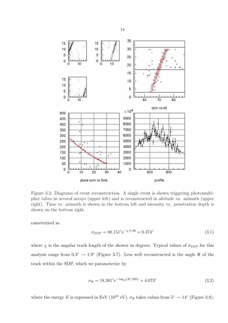
Figure 3.2: Diagrams of event reconstruction. A single event is shown triggering photomulti-plier tubes in several arrays (upper left) and is reconstructed in altitude vs. azimuth (upperright). Time vs. azimuth is shown in the bottom left and intensity vs. penetration depth isshown on the bottom right.

rameterized as

σSDP = 88.151◦e−χ/1.96 + 0.374◦ (3.1)

where χ is the angular track length of the shower in degrees. Typical values of σSDP for this

analysis range from 0.3◦ → 1.9◦ (Figure 3.7). Less well–reconstructed is the angle Ψ of the

track within the SDP, which we parameterize by

σΨ = 18.381◦e− log10(E/.691) + 4.073◦ (3.2)

where the energy E is expressed in EeV (1018 eV). σΨ takes values from 5◦ → 14◦ (Figure 3.8).

19

Figure 3.3: The energies of events reconstructed using monocular and stereo techniques sepa-rately.

Ψ is not as well–reconstructed because of our monocular vision, which experiences more error in

any measurement requiring depth perception. Uncertainties in σSDP and σψ are approximately

7.5% [23]. A few events with their “error ellipses” are shown in Figure 3.9.

Density Skymaps

In Figure 3.10, we plot the skymap formed from the arrival direction of events in the

present dataset. Each event’s “error ellipse” is represented by generating 1,000 points per

event, distributed according to the Gaussian error model of Equations 3.1 and 3.2. Note the

bin size in this plot and in the subsequent analysis is chosen to be constant in the Cartesian

projection of this polar coordinate system, and approximately 1◦ × 1◦.

We next discuss the Monte Carlo technique by which we evaluate the significance of fluc-

tuations in the skymap as well as our sensitivity to pointlike behavior in arrival direction.

20

Figure 3.4: Comparison of HiRes–I data(points) and Monte Carlo (solid histogram)distributions in zenith angles (degrees).

Figure 3.5: Comparison of HiRes–I data(points) and Monte Carlo (solid histogram)distributions in distance to shower core (km).

Figure 3.6: The geometry of reconstruction for a monocular air fluorescence detector.

21

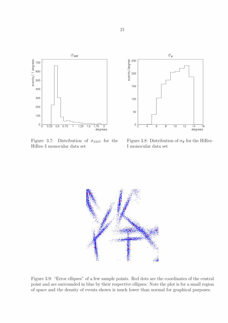
Figure 3.7: Distribution of σSDP for theHiRes–I monocular data set

Figure 3.8: Distribution of σΨ for the HiRes–I monocular data set

Figure 3.9: “Error ellipses” of a few sample points. Red dots are the coordinates of the centralpoint and are surrounded in blue by their respective ellipses. Note the plot is for a small regionof space and the density of events shown is much lower than normal for graphical purposes.

22

Figure 3.10: Skymap of arrival directions of events in the the HiRes–I monocular dataset,plotted in polar projection, equatorial coordinates. Each HiRes event is represented by 1,000points randomly thrown according to the elliptical Gaussian error model of Equations 3.1 and3.2. The bin size in this plot (and all similar plots) is approximately 1◦ × 1◦.

23

CHAPTER 4

ISOTROPIC BACKGROUND, COMPARISON TO REAL DATA,

SIMULATION OF POINT–LIKE SOURCES

To identify a point-like source in Figure 3.10, we must first understand the statistical

fluctuations that might mimic a point-like source in an isotropic sky. We study these fluctua-

tions by using Monte Carlo techniques to create isotropic “data sets” with the same detector

exposure as the HiRes-I monocular data set. Then, we use similar Monte Carlo techniques

to simulate data sets containing pointlike sources, to arrive at a set of criteria by which we

may confidently identify true sources with a small likelihood of obtaining false positives from

background fluctuations.

The Monte Carlo Generated Isotropic Background

To create isotropic background data sets, we first determine the energy of the incident

particle by using the exposure corrected energy spectrum observed by the Fly’s Eye stereo

experiment. By using the Fly’s Eye energy spectrum, we assume the energy spectrum is the

same at all positions in the sky – thus, we assume an isotropic distribution for events possessing

the spectrum and composition reported by the stereo Fly’s Eye experiment [27, 28]. The arrival

directions of these events are then simulated at all possible viewing angles. Showers which

pass the initial cuts and profile–constrained fit discussed in Chapter 3 will possess the same

aperture in both energy and the viewing angles of HiRes–I. We then use a database of detector

on-times, given by the timing of events in the real data, to calculate the time of arrival of the

Monte Carlo events. Mirrors in the ring will sometimes require repairs and be shut off, so

we exclude any events whose arrival direction would only be successfully reconstructed by a

non-functioning mirror at the time.

A total of 1,000 isotropic data sets with the same exposure and number of events as the

HiRes–I monocular data were generated for comparison studies. Further discussion of this

Monte Carlo can be found in the References [20, 29]. Comparison of the real data to our

isotropic background in zenith angle, Figure 3.4, and distance to the shower core, Figure 3.5,

24

show good agreement, indicating successful simulation of an isotropic background. In Fig-

ures 4.1 and 4.2 we compare the data and Monte Carlo distributions of events in the variables

RA and DEC, respectively. Ground arrays typically show an even exposure in RA, but we

do not because our nitrogen fluorescence detector operates only at night. Winter nights at

our latitude (40.2◦) are measurably longer than summer nights. At midnight on the summer

solstice, 17.5 hrs RA is at zenith (approximately), while 5.5 hrs RA is at zenith during the

winter solstice.

Figure 4.1: Comparison of HiRes–I data (points) and Monte Carlo (solid histogram) distribu-tions in right ascension (RA).

Figure 4.2: Comparison of HiRes–I data (points) and Monte Carlo (solid histogram) distribu-tions in declination (DEC).

25

Isotropic Background Corrected Skymaps

In order to understand the significance of the fluctuations in Figure 3.10, we compare the

data on a bin-by-bin basis to the 1,000 simulated datasets. Defining NDATA as the bin density

of the data, NMC as the bin density of the simulated isotropic datasets, and N as the number

of simulated isotropic datasets (1,000), the variable

χ1 =(NDATA − 〈NMC〉)

σMC

(4.1)

provides a measure of the fluctuation per bin, where σMC is the standard deviation of the

Monte Carlo bin density

σMC =

√√√√ 1

N − 1

N∑i=1

(NMC,i − 〈NMC〉)2 (4.2)

(Figure 4.3). 〈NMC〉, Figure 4.4, is the average bin density of the simulated isotropic datasets

and graphically demonstrates HiRes exposure as a function of position.

Figure 4.3: σMC (Equation 4.2) distribution,the standard deviation of the Monte Carlobin density.

Figure 4.4: 〈NMC〉 distribution graphicallydemonstrates the effects of summer/winternights on our exposure.

26

Figure 4.5 shows the distribution of χ1 as a function of position in the sky for the HiRes–

I monocular dataset as extracted from this technique. The bin-by-bin distributions of χ1

are non-Gaussian (Figure 4.6) in a manner that varies as a function of position in the sky.

Thus it is necessary to develop a technique to evaluate the significance of possible sources.

Our technique uses the χ1 information in neighboring bins to pick out significant fluctuations

above background from the skymap. The parameters in the technique are tuned on simulated

pointlike sources.

Figure 4.5: χ1 (Equation 4.1) distribution for the HiRes-I monocular data set. This plot is(Figure 3.10 - Figure 4.4)/Figure 4.3.

27

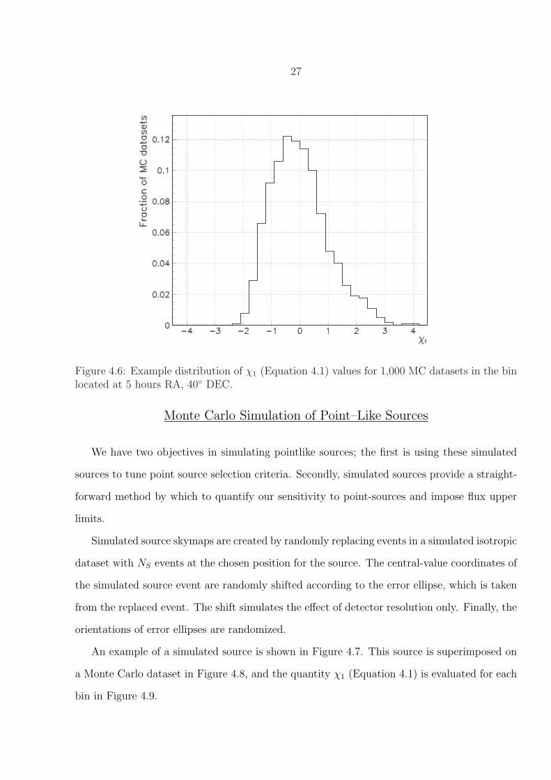
Figure 4.6: Example distribution of χ1 (Equation 4.1) values for 1,000 MC datasets in the binlocated at 5 hours RA, 40◦ DEC.

Monte Carlo Simulation of Point–Like Sources

We have two objectives in simulating pointlike sources; the first is using these simulated

sources to tune point source selection criteria. Secondly, simulated sources provide a straight-

forward method by which to quantify our sensitivity to point-sources and impose flux upper

limits.

Simulated source skymaps are created by randomly replacing events in a simulated isotropic

dataset with NS events at the chosen position for the source. The central-value coordinates of

the simulated source event are randomly shifted according to the error ellipse, which is taken

from the replaced event. The shift simulates the effect of detector resolution only. Finally, the

orientations of error ellipses are randomized.

An example of a simulated source is shown in Figure 4.7. This source is superimposed on

a Monte Carlo dataset in Figure 4.8, and the quantity χ1 (Equation 4.1) is evaluated for each

bin in Figure 4.9.

28

Figure 4.7: Skymap of example source without an isotropic background. The source containsNS = 25 events and has been inserted at 5 hours RA, 40◦ DEC.

29

Figure 4.8: Skymap of arrival directions of events for a Monte Carlo dataset, having the sameoverall exposure as the HiRes–I monocular dataset, with a 25 event source superimposed at 5hours RA, 40◦ DEC.

30

Figure 4.9: χ1 (Equation 4.1) for NS = 25 event source inserted in a simulated isotropicdataset. The source has been inserted at 5 hours RA, 40◦ DEC.

31

CHAPTER 5

CRITERIA FOR DECLARATION OF A POINT SOURCE

We now describe a procedure by which we can identify pointlike behavior in arrival direction

(for example, the simulated source of Figures 4.7, 4.8, and 4.9) while simultaneously rejecting

false positives arising from fluctuations of the background.

Due to detector resolution, it is desirable that we search for sources by considering points

over an extended angular region. We consider a “search circle” of radius R, where R is

expressed as an angle in degrees. Within the search circle, we count the fraction of bins F

having a χ1 value greater than some threshold χTHR. The parameters R and χTHR are chosen

to optimize the signal size, and a cut is chosen on the fraction F which reduces the probability

of false positives to an acceptable level.

Our maximum sensitivity to pointlike behavior in arrival direction, given the HiRes–I

pointing uncertainty, has been determined empirically to require a search circle of R = 2.5◦,

and a value χTHR = 4. (In the case in which the bin densities are normally distributed, this

corresponds to 4 Gaussian σ’s.) The optimum values for these parameters were determined

by simulating sources at various locations in the sky and maximizing our sensitivity to these

sources. The values are found to be largely insensitive to the position in the sky and the

number of events in the source. Additionally, small variations in either of these parameters do

not have a significant impact on our results.

Due to low statistics at the edge of HiRes’ acceptance, we consider only search circles with

centers at declinations greater than 0◦. That is, we only search for sources north of the celestial

equator. Approximately 10% of HiRes events are south of the equator, however these events

can contribute to the search if their error ellipses extend north of DEC = −2.5◦.

In Figure 5.1, we have plotted for each bin the fraction F , for R = 2.5◦ and χTHR = 4,

of the simulated point source of Figure 4.8. The simulated source stands out clearly in this

figure.

32

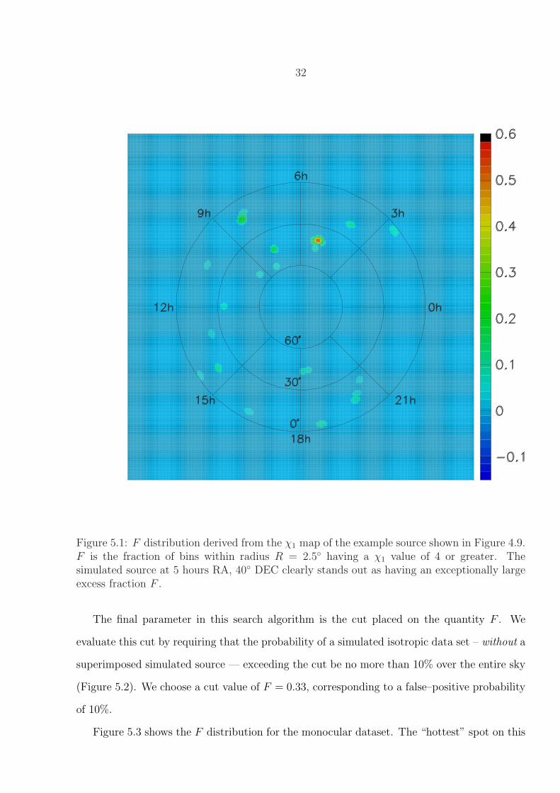
Figure 5.1: F distribution derived from the χ1 map of the example source shown in Figure 4.9.F is the fraction of bins within radius R = 2.5◦ having a χ1 value of 4 or greater. Thesimulated source at 5 hours RA, 40◦ DEC clearly stands out as having an exceptionally largeexcess fraction F .

The final parameter in this search algorithm is the cut placed on the quantity F . We

evaluate this cut by requiring that the probability of a simulated isotropic data set – without a

superimposed simulated source — exceeding the cut be no more than 10% over the entire sky

(Figure 5.2). We choose a cut value of F = 0.33, corresponding to a false–positive probability

of 10%.

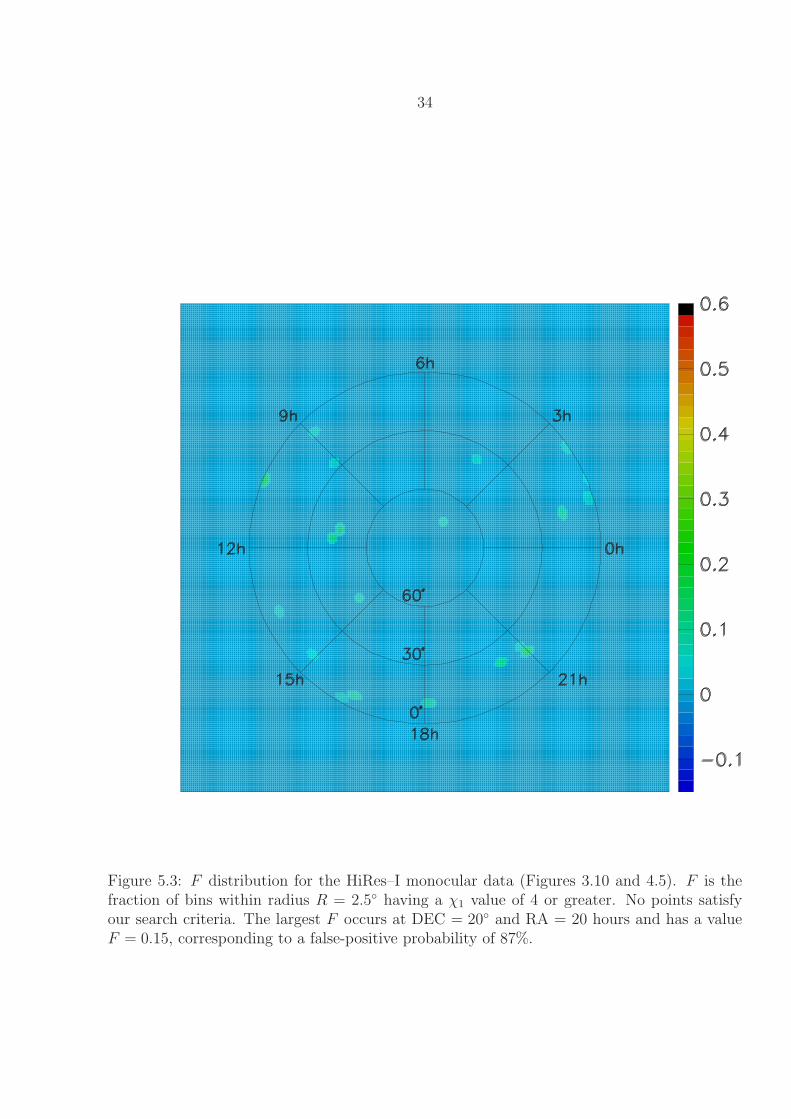
Figure 5.3 shows the F distribution for the monocular dataset. The “hottest” spot on this

33

graph, near DEC = 20◦ and RA = 20 hours, has a value F = 0.15. 87% of simulated isotropic

datasets have F ≥ 0.15 (see Figure 5.2). We conclude that our observation is consistent with

a fluctuation from an isotropic background.

Figure 5.2: Occurrence rate of false positives versus F for a 2.5◦ search circle and χ1 thresholdof 4. A cut at F = 0.33 corresponds to a false-positive probability of 10%. The maximumvalue of F encountered in the real data, .15, corresponds to a false positive probability of 87%.

Next, we evaluate the corresponding sensitivity and flux upper limits as a function of

position in the sky.

34

Figure 5.3: F distribution for the HiRes–I monocular data (Figures 3.10 and 4.5). F is thefraction of bins within radius R = 2.5◦ having a χ1 value of 4 or greater. No points satisfyour search criteria. The largest F occurs at DEC = 20◦ and RA = 20 hours and has a valueF = 0.15, corresponding to a false-positive probability of 87%.

35

CHAPTER 6

SENSITIVITY, UPPER LIMITS

Having determined that no evidence exists in the HiRes–I monocular dataset for pointlike

excesses over isotropy, we now seek to determine our sensitivity and place upper limits on the

flux from such sources as a function of position in the sky.

We chose a grid of locations (Table 6.1) distributed evenly across the Northern Hemisphere,

with lines of RA approximately corresponding to the HiRes solstices and equinoxes. At each

grid point, we generate 400 point like sources superimposed on independent isotropic back-

grounds, where each source data set has the same total number of events as the HiRes data.

The number of events in each source is distributed in a poisson manner, where the mean value

over the 400 sources is termed 〈NS〉. 〈NS〉 is then varied at each location.

We then determine the percentage of trials at each location for which our reconstruction

algorithm “finds” a source of size 〈NS〉. The algorithm will “find” a source if it fluctuates

above the cut on F , where the numerical cut value is dependent on whether we’re calculating

sensitivities or upper limits. The value of 〈NS〉 for which signal was declared for 90% or

better of the trials was termed NF , where F corresponds to the cut value on F . Sensitivity

is given by the value of N.33 that satisfies the criteria for positive signal defined in Chapter 5

(χ1 > 4, r ≤ 2.5◦, F > .33). If a source of size N.33 existed in the real data, our probability of

declaring positive signal would be 90%, yielding the 90% c.l. sensitivity of our experiment.

However, since the real data never fluctuated above F = .33, we calculate the size of source

that yields the F measured in the real data to determine our upper limit. We calculate source

size upper limits by setting our cut on F to the highest value that occurred in the real data,

F = .15. N.15 is the value of 〈NS〉 for which signal was declared for F > .15 in 90% or better

of the trials. N.15 gives the upper limit because a signal of size N.15 was not measured in the

real data. With 90% certainty, experiments identical to HiRes–I will not measure a source

of size greater than this upper limit. We use the maximum value of F = .15 for all the grid

points instead of the value in the real data at each grid point because we want an upper limit

that can be smoothly interpolated between grid points. This results in a higher upper limit

36

than what could be calculated for locations in the sky where F is significantly less than .15

in the real data. The systematic uncertainty in the calculation of NF , due to uncertainties in

the error ellipses, is ≤ 1 event.

To calculate the detector exposure [29] for point sources at the grid points, Monte Carlo

events are generated at the grid points, assigned a time from the distribution of HiRes de-

tector ontimes, and projected towards the detector aperture. Local coordinates and times

are determined, then the event is paired with a shower from the Monte Carlo event library

having similar local coordinates. An attempt is then made to reconstruct the Monte Carlo

event with the profile–constrained fitting technique. The exposure, defined as the fraction of

events reconstructed multiplied by the detector aperture (area) and time, can then be used to

determine sensitivity and flux upper limits for each of the grid locations. These exposures are

listed in Table 6.1. Finally, 90% confidence level flux sensitivities and upper limits are simply

NF divided by the exposure at each grid point.

Sensitivity

The distribution of N.33 at the grid points are illustrated in Figure 6.1. 90% confidence

level flux sensitivities are N.33 divided by the exposure (Table 6.1 and Figure 6.2).

Upper Limits

The distribution of N.15 at the grid points are shown in Figure 6.3. These results allow us

to rule out the existence of pointlike sources of strength N.15 at the grid locations with 90%

confidence level. Flux upper limits are N.15 divided by the exposure (Table 6.1 and Figure 6.4).

The largest flux upper limit across the entire sky is 0.8 events/km2yr. Thus, we rule out

the existence of pointlike behavior in arrival direction of cosmic rays of energy above 1018.5

eV with flux greater than 0.8 events/km2yr at 90% confidence level and place more stringent

limits as a function of position in Figure 6.4.

Finally, Cygnus X-3 (RA 20.5 hours, DEC 40.7◦) is very near the grid point at RA 20.5

hours, DEC 45◦, allowing us to place a flux upper limit from Cygnus X-3 of 0.5 events/km2yr

with 90% confidence.

37

Figure 6.1: Numerical values of N.33 (events)at 21 grid points in the Northern Hemi-sphere.

Figure 6.2: Flux sensitivity (events/km2yr)at 21 grid points in the Northern Hemi-sphere.

Figure 6.3: Numerical values of N.15 (events)at 21 grid points in the Northern Hemi-sphere.

Figure 6.4: Flux upper limit (events/km2yr)at 21 grid points in the Northern Hemi-sphere.

38

DEC RA Exposure Sensitivity Upper Limit

(deg) (hours)N.33 N.15 (km2yr) (events/km2yr) (events/km2yr)

2.5 hrs 23 16 34.2 .7 .55.5 hrs 24 19 36.6 .7 .58.5 hrs 22 16 34.3 .6 .511.5 hrs 20 16 24.5 .8 .7

15◦ 14.5 hrs 18 14 21.9 .8 .617.5 hrs 18 13 16.7 1.1 .820.5 hrs 17 13 21.1 .8 .623.5 hrs 21 16 26.7 .8 .62.5 hrs 26 20 49.7 .5 .45.5 hrs 29 22 56.6 .5 .48.5 hrs 25 20 48.5 .5 .411.5 hrs 24 18 41.2 .6 .4

45◦ 14.5 hrs 21 15 33.5 .6 .417.5 hrs 21 16 24.9 .8 .620.5 hrs 21 16 30.3 .7 .523.5 hrs 24 18 41.5 .6 .45.5 hrs 29 21 59.8 .5 .411.5 hrs 28 21 50.5 .6 .4

75◦ 17.5 hrs 26 19 38.6 .7 .523.5 hrs 26 20 47.2 .6 .4

90◦ N/A 31 23 53.8 .6 .4

Table 6.1: Locations of grid points for flux upper limits, with signal strength N.33 and N.15,exposures (with uncertainty 5% from Monte Carlo statistics), calculated sensitivity, and fluxlimits.

39

CHAPTER 7

CONCLUSIONS

We have conducted a search for pointlike excesses in the arrival direction of ultra–high

energy cosmic rays with energy exceeding 1018.5 eV in the northern hemisphere. We place an

upper limit of 0.8 events/(km2 yr) (90% c.l.) on the flux from such sources across the entire

sky and place more stringent limits as a function of position. We also determine sensitivity as

a function of position in the sky, and place an upper limit on the flux from the a priori chosen

direction of the x-ray binary Cygnus X-3 of 0.5 events/(km2 yr) (90% c.l.). The HiRes–I

monocular data is thus consistent with the null hypothesis for pointlike excesses of neutral

primary cosmic rays in this energy range.

Additional Capabilities of this Analysis Technique

The technique of simulating sources, tuning selection criteria on these sources, and de-

termination of sensitivity and upper limits given a null result can be adapted for multiple

analyses: 1) a focused search for a pointlike excess in a limited region of the sky, 2) a search

for small extended sources, and 3) a search for charged events originating from a pointlike

source.

Search for Pointlike Excess in a Small Region

There are numerous high energy astrophysical objects that could be potential point sources

of neutrally charged UHECR, such as Cygnus X-3, M87, or Centaurus A. The region of the

AGASA “triplet” is also of interest. A simple extension of this analysis would be to perform the

same study around one or more chosen regions. This is perhaps the most powerful and easiest

adaptation of the technique outlined in this thesis. The technique for generating point sources

would be the same. R and χTHR could be tuned to maximize sensitivity to generated pointlike

sources in that region. Over a smaller region, there is a substantial decrease in false positive

probability for given cuts on F, therefore, sensitivity levels could be dramatically increased.

The technique would require simulation of substantially more Monte Carlo isotropic data sets

40

so distributions in F are smooth. Early attempts yielded plots of false positive probability vs.

F (similar to Figure 5.2) with “steps” in the plot - indicating a need for more isotropic data

sets and finer angular resolution. Unfortunately, this focused search can be applied only to a

limited number of potential sources because a heavy statistical penalty is accrued by searching

for too many. However, this extension could provide a powerful way to confirm or refute the

most debated point-like sources.

Search for Small Extended Sources

Another relatively easy search would be for small extended sources. There are a number

of astrophysical objects of interest which subtend a measurable, but small, angle in the sky.

Andromeda, the nearest galaxy to us, subtends approximately 3◦ x 1◦ in our sky. The galactic

core has many interesting features at various angular scales; they subtend the sky anywhere

from 1◦ x 1◦ (often referred to as the galactic nucleus) to 10◦ x 10◦. The most energetic nearby

galaxy, Centaurus A, subtends roughly 1◦ x 1◦. A simple extension to the analysis would

be to simulate sources including detector resolution and astrophysical “smearing,” where the

“smearing” factor is due to the physical size of the object as it appears in our sky. This analysis

should be performed in a specific region because the amount of “smearing” one expects will

be dependent on the candidate source. By performing the analysis in a particular region,

sensitivity would increase from the regionally reduced false-positive probability. Once again,

the analysis would be for contributions from neutral primaries only and the same statistical

penalty applies when the search is performed in too many regions.

Including Charged Particles from Point Sources

Charged events originating from point sources are thought to experience significant mag-

netic deflection as they traverse through the galaxy. This deflection could be modelled as a

“halo” surrounding the source, perhaps with a neutral contribution from the center. Instead

of using one R, the analysis would require an Rmin and Rmax for the “halo” and perhaps an

Rinternal to model neutral particle contributions. Unfortunately, there are many requirements

which are hard to fulfill for simulating this type of source. A general class of source candidate

would have to be chosen because the magnetic fields internal to the galaxy are substantially

41

different than those external. General classes could include sources within the galactic core

or extragalactic sources positioned such that the distance and angle of traverse through the

galaxy is known. It requires specific information about the magnitude of galactic and extra-

galactic magnetic fields – quantities that are not well agreed upon. Additionally, the analysis

would have to be done for a specific particle type as a function of energy because the degree of

bending will be highly dependent on the energy of the particle and its composition. It would

require a data set substantially larger than HiRes–I monocular data because the number of

point-source events would be comparatively small for each energy range, resulting in poor

sensitivity in small data sets. For all these reasons, this possible extension to the analysis is

the least feasible.

The Future of UHECR Studies

The next two projects in UHECR are the Pierre Auger Observatory (Auger) and the

Telescope Array (TA). Auger is an international project hosted through Fermilab and TA is a

collaboration primarily between members of the AGASA and HiRes groups. Both experiments

are hybrid detectors, utilizing the technologies of ground arrays and fluorescence detection. It

is hoped that as hybrid detectors, they will resolve the disparity between AGASA and HiRes

energy spectrums.

Auger, based in Argentina, will be the first experiment with significant UHECR statistics

in the southern hemisphere, allowing coverage of the other half of our sky. Auger is currently

operational (Figure 7.1) and when complete, will boast the largest aperture yet. They project

their data set will contain more events than HiRes monocular at 1019 eV or more some time

during the summer of 2005 [30]. Their detector uses Cerenkov light water tanks to detect

showers on the ground which operate at all times and several nitrogen fluorescence detectors

looking out at the horizon which operate at night. Multiple fluorescence detectors will allow

Auger to have a stereo dataset with better angular resolution than each individual detector.

Auger’s detectable energy range is around 1019 eV and above, allowing them to have excellent

resolution of behavior near the GZK feature. Hopefully, Auger will be able to definitively

state if the GZK feature is there as theory predicts. However, since Auger does not detect

42

lower energy events, they may be unable to resolve the full “ankle” structure (see Chapters 1

and 2), and almost certainly won’t measure the “second knee.”

Figure 7.1: Map of the Pierre Auger Observatory, a hybrid detector in the southern hemisphere(Argentina). Dots show ground detector locations and the green rays show fluorescence detec-tor viewing angles. The blue outline shows components of the observatory that were deployedand mostly operational as of December 2004.

TA will have a smaller aperture than Auger, but is projected to resolve events with energies

lower than 1017 eV and as high as 1020.5 eV, allowing a complete spectrum, although with

reduced statistics at the highest energies compared to Auger. TA obtains this extreme energy

range by using existing geography in Millard County, Utah. The ground detectors, scintillator

plates which detect shower particles directly, are at low elevations in the flat valley floors,

while the nitrogen fluorescence detectors will be on the top of local mountains (Figure 7.2).

This allows detection of shower maximums at low and high altitudes, where the location of

shower maximum is determined by the energy of the incident cosmic ray (see Chapter 1). TA

is projected to resolve the “second knee,” a structure that so far has not been well-measured

by any experiment, the full “ankle” structure, and the GZK feature. TA should also have

better data for determining the compositional changes of UHECR than Auger because it will

be the only single experiment with data for the full energy range shown in Figure 1.4. Finally,

TA angular resolution should be the best achieved yet because of multiple detectors allowing

stereo reconstruction and observation of a significant portion of the shower as it develops (see

Chapter 3).

43

Figure 7.2: Map of the Telescope Array, a proposed hybrid detector. TA uses HiRes fluores-cence detectors at high elevation (red squares) and a ground array at lower elevation (bluedots).

Auger plans to eventually construct a northern hemisphere site for full sky coverage. It is

possible that TA and Auger may merge to defray costs. Construction on the TA ground array

from Japanese grants has begun while funding for the nitrogen fluorescence detectors is being

sought from the USA.

44

REFERENCES CITED

[1] K. Greisen, Phys. Rev. Lett. 16 (1996) 748.

[2] G.T. Zatsepin and V.A. K’uzmin, Pis’ma Zh. Eksp. Teor. Fiz. 4 (1966) 114 [JETP Lett.4 (1966) 78].

[3] R.U. Abbasi et al., astro-ph/0501317, submitted to Phys. Lett. B (2005).

[4] D.J. Bird et al., Phys. Rev. Lett. 71 (1993) 3401.

[5] M. Takeda et al., Astropart. Phys. 19 (2003) 447.

[6] M. Ave et al., Astropart. Phys. 19 (2003) 47.

[7] N. Hayashida et al., Astropart. Phys. 10 (1999) 303.

[8] G.L. Cassiday et al., Phys. Rev. Lett. 62 (1989) 383.

[9] M. Teshima et al., Phys. Rev. Lett. 64 (1990) 1628.

[10] M.A. Lawrence et al., Phys. Rev. Lett. 63 (1989) 1121.

[11] A. Borione et al., Phys. Rev. D55 (1997) 1714.

[12] T. Doi et al., Proc. 24th ICRC (Rome) 2 (1995) 804.

[13] N. Hayashida et al., Phys. Rev. Lett. 77 (1996) 1000.

[14] M. Takeda et al., Proc. 27th ICRC (Hamburg) (2001) 345.

[15] M. Teshima et al., Proc. 28th ICRC (Tsukuba) (2003) 437.

[16] T. Abu Zayyad et al., Proc. 26th ICRC (Salt Lake City) 5 (1999) 349.

[17] T. Abu-Zayyad, Ph.D. Thesis, University of Utah (2000).

[18] X. Zhang, Ph.D. Thesis, Columbia University (2001).

[19] R.U. Abbasi et al., Phys. Rev. Lett. 92 (2004) 151101.

[20] R. Abbasi et al., Astropart. Phys. 21 (2004) 111.

[21] G.R. Farrar and T. Piran, astro-ph/0010370.

[22] R.U. Abbasi et al., submitted to Astropart. Phys. (2005).

[23] R.U. Abbasi et al., Astroparticle Physics 22 (2004) 139.

[24] R.U. Abbasi et al., Astrophys. J. L73 (2004) 610.

[25] L.M. Widrow, Rev. Mod. Phys. 74 (2003) 775.

[26] T. Gaisser and A.M. Hillas, Proc. 15th ICRC (Plovdiv) 8 (1977) 353.

45

[27] D.J. Bird et al., Proc. 23rd ICRC (Calgary) 2 (1993) 38.

[28] D.J. Bird et al., Astrophys. J. 424 (1994) 491.

[29] B. Stokes, Ph.D. Thesis, University of Utah (2005).

[30] http://www.auger.org/