seakeeping enhancement by lengthening a ship
TRANSCRIPT
IN DEGREE PROJECT MECHANICAL ENGINEERING,SECOND CYCLE, 30 CREDITS
, STOCKHOLM SWEDEN 2018
Seakeeping enhancement by lengthening a ship
RÉMI CLAUDEL
KTH ROYAL INSTITUTE OF TECHNOLOGYSCHOOL OF ENGINEERING SCIENCES

© Naval Group SA All rights reserved 2018.
Both the content and the form of this document/software are the property of Naval Group and/or of third party. It is formally prohibited to use, copy, modify, translate, disclose or perform all or part of this document/software without obtaining Naval Group’s prior written consent or authorization. Any such unauthorized use, copying,
modification, translation, disclosure or performance by any means whatsoever shall constitute an infringement punishable by criminal or civil law and, more generally, a breach of Naval Group’s (or name of the relevant subsidiary company) rights.
NON SENSITIVE
MASTER DEGREE PROJECT SEAKEEPING ENHANCEMENT BY LENGTHENING A SHIP
Degree project in Naval Architecture : course code SD271X
Author : Rémi Claudel
Company supervisor : Thierry Guézou
Kungliga Tekniska Högskolan (KTH) supervisor : Anders Rosén
Degree project from 03/07/2017 to 08/12/2017

Master Degree Project Report
Seakeeping enhancement by lengthening a ship
Page 3/83
© Naval Group SA property, 2018, all rights reserved
NON SENSITIVE
Abstract
In this study, a tentative assessment of a passive solution for pitch decrease, namely the increase
in length of the studied ship, is made. The hull form of the lengthened version of the ship is
derived from the reference hull form after utilization of Lackenby’s sectional area curve
transformation through a prismatic coefficient change (Reference [3]), and utilization of a
sectional area curve “swinging” induced by a change of longitudinal position of the centre of
buoyancy. Following this, and after a complementary mass estimate of the lengthened version,
seakeeping calculations are made and show a significant decrease in pitch, from almost 35% for
low sea states to 20% for relatively high sea states. To conclude this study, operability for classic
NATO frigate missions have been calculated and the decrease in pitch induces a slight gain in
operability for the lengthened version.

Master Degree Project Report
Seakeeping enhancement by lengthening a ship
Page 4/83
© Naval Group SA property, 2018, all rights reserved
NON SENSITIVE
Acknowledgments
I would like to express my deep gratitude to Thierry Guézou for having given me the opportunity
to work with him in Naval Group surface ships preliminary projects department for these few
months.
I would also like to thank everyone from the different services who took the time to teach me
and answer my questions, in particular Benoît Fumery, Philippe Fleury, Pierre Vonier, Pierre-
Marie Guillouet and Alex Riu.
Lastly, I would like to thank Pierre Raspic and Roger Le Doussal for enlivening the life at the
office as well as my fellow interns.

Master Degree Project Report
Seakeeping enhancement by lengthening a ship
Page 5/83
© Naval Group SA property, 2018, all rights reserved
NON SENSITIVE
Table of contents
1 LIST OF SYMBOLS .............................................................................................. 7
2 INTRODUCTION ................................................................................................... 9
2.1 Project Topic ................................................................................................................................................... 9
2.2 Motivation ....................................................................................................................................................... 9
2.3 State of the art ................................................................................................................................................ 9
2.4 Study steps .....................................................................................................................................................10
3 LENGTHENED HULL FORM ...............................................................................11
3.1 Reference ship ................................................................................................................................................11
3.2 “Frigate+” hullform main characteristics calculations ..............................................................................11
3.3 Sectional area curve transformation ...........................................................................................................13 3.3.1 Transformation by variation of the prismatic coefficient .......................................................................13 3.3.2 Transformation by variation of the centre of buoyancy .........................................................................16
3.4 Hull form transformations ...........................................................................................................................18 3.4.1 Modification of cross section shapes .....................................................................................................19 3.4.2 Modification of the cross section longitudinal positions .......................................................................21
3.5 Structure ........................................................................................................................................................22 3.5.1 Midship section strengthening ...............................................................................................................22 3.5.2 Displacement estimate ...........................................................................................................................24
4 SEAKEEPING AND OPERABILITY ....................................................................26
4.1 Precal_R seakeeping results .........................................................................................................................26 4.1.1 Transfer functions ..................................................................................................................................27 4.1.2 Pitch .......................................................................................................................................................31
4.2 Calculations et Formulas used in Precal_R output data post processing .................................................35 4.2.1 Wave spectrum ......................................................................................................................................35 4.2.2 Motions and derivatives .........................................................................................................................37 4.2.3 Emergence and Slamming .....................................................................................................................38 4.2.4 Motion Sickness Incidence (MSI) .........................................................................................................40 4.2.5 Motion Induced Interruptions (MII) ......................................................................................................41 4.2.6 Lateral Force Estimator .........................................................................................................................42
4.3 PRECAL_R post processing Excel tool .......................................................................................................43
4.4 Software limitations ......................................................................................................................................47 4.4.1 Transfer functions values .......................................................................................................................47 4.4.2 Roll damping fins implementation .........................................................................................................49

Master Degree Project Report
Seakeeping enhancement by lengthening a ship
Page 6/83
© Naval Group SA property, 2018, all rights reserved
NON SENSITIVE
4.5 Operability results .........................................................................................................................................50 4.5.1 Pitch .......................................................................................................................................................50 4.5.2 Transit and Patrol mission .....................................................................................................................52 4.5.3 Speed maintaining in heavy seas ...........................................................................................................53 4.5.4 Helicopter and drone operations ............................................................................................................54 4.5.5 Helicopter and drone handling and helicopter armament ......................................................................55 4.5.6 Crafts launch by the side ........................................................................................................................56 4.5.7 Replenishment at sea .............................................................................................................................57 4.5.8 Replenishment at sea by helicopter ........................................................................................................58 4.5.9 Vertical launchers operation ..................................................................................................................59 4.5.10 Torpedo tubes operation ....................................................................................................................60 4.5.11 Main gun operation ...........................................................................................................................61
5 RESISTANCE ......................................................................................................63
5.1 Using existing reference measures ...............................................................................................................63
5.2 Fung Method ..................................................................................................................................................65
5.3 Speed and Power ...........................................................................................................................................67
6 COSTS .................................................................................................................70
7 CONCLUSION .....................................................................................................71
8 REFERENCES .....................................................................................................72
9 APPENDICES ......................................................................................................74
9.1 Appendix 1: Proof of the variation of LCB via a « swinging » of the sectional area curve .....................74
9.2 Appendix 2: Formulas for the deformation of a section ............................................................................76
9.3 Appendix 3: Hull girder strengthening effective length .............................................................................81

Master Degree Project Report
Seakeeping enhancement by lengthening a ship
Page 7/83
© Naval Group SA property, 2018, all rights reserved
NON SENSITIVE
1 List of Symbols
Am Midship section underwater area
B Waterline breadth
Boa Overall breadth
C Depth
Cb Block coefficient
Cm Midship section coefficient
Cp Prismatic coefficient
CWS Wetted surface coefficient
D1 Longitudinal motion
D2 Lateral motion
D3 Vertical motion
Fn Froude number
g Gravitational acceleration
h Height of an operator’s centre of gravity
H Significant wave height
IE Deadrise angle
KG Vertical position of the centre of gravity of the ship relatively to the keel
l Half width between an operator’s feet
L Waterline length
Laft Length aft of the midship section
Lfor Length forward of the midship section
Loa Overall length
Lpp Length between perpendiculars
LCB Longitudinal position of the centre of buoyancy from the aft perpendicular
LCG Longitudinal position of the centre of gravity rom the aft perpendicular
LFE Lateral Force Estimator
Mf Bending moment
MII Motion Induced Interruptions
MSI Motion Sickness Incidence
P Power
Rf Viscous resistance

Master Degree Project Report
Seakeeping enhancement by lengthening a ship
Page 8/83
© Naval Group SA property, 2018, all rights reserved
NON SENSITIVE
RR Residuary resistance
Rt Total resistance
Rts Specific resistance
RMS Root Mean Square
S Midship section structure cross section area
S(ω) Wave spectrum
T Draught
Tm Mean wave period
Tp Wave spectrum peak period
V Speed
WS Wetted surface
X Longitudinal position
XG Longitudinal position of the centre of gravity
Y Lateral position
YG Lateral position of the centre of gravity
Z Vertical position
ZG Vertical position of the centre of gravity
Δ Displacement
η Propulsive system efficiency
η1 Surge
η2 Sway
η3 Heave
η4 Roll
η5 Pitch
η6 Yaw
µ Wave heading
ρ Seawater density
σx RMS of x
ω Wave angular frequency
ωe Encounter frequency
∇ Displaced volume

Master Degree Project Report
Seakeeping enhancement by lengthening a ship
Page 9/83
© Naval Group SA property, 2018, all rights reserved
NON SENSITIVE
2 Introduction
2.1 Project Topic
The main objective of this project is to assess the seakeeping, operational and cost impact of
increasing the length of a ship beyond that which results from a traditional spiral design process
whereby a ship inner volume is solely defined by its systems physical integration requirements.
It is proposed that this increase in length is achieved by adding to a ship platform a forward
empty section which sole purposes are to increase the ship waterline length and its forward
reserve of buoyancy. It is not to be outfitted; the ship internal arrangement remains within the
length required for physical integration and constraints.
This study has been undertaken by establishing a comparison between a parent (reference) ship
and a lengthened version such as described above. The other ship parameters are not changed or,
if it cannot be avoided, the least possible.
This length increase leads to a decrease in heave and pitch and so to better seakeeping
characteristics (less slamming, propeller emergence, green water on deck…) which allows the
ship to operate at higher speeds in heavy seas. However, this modification incurs a building cost
increase. So, in addition to quantifying the seakeeping characteristics enhancement of the
modified ship; construction and operational cost increase are also estimated in order to answer
the question: does seakeeping improvement justify cost increases?
2.2 Motivation
Speed at sea is imperative for the diverse missions of the French Navy as it is detailed by
Frigate Captain Laurent Célérier (Reference [1]). Be it for maritime traffic protection via anti-
piracy patrols, for natural resources protection via the interception of poachers and terrorists, for
the fight against illegal traffic, for the reaction to crisis outbreaks or during stabilization stages
or simply for self-defense, the maximum speed that a naval ship can achieve is a key operational
factor. Right now, according to him, this speed is satisfactory in calm water. In heavy seas,
however, ships cannot reach this same maximum speed. This explains the interest for a ship that
would have a better seakeeping and could therefore travel faster in heavy sea and keep on
operating in heavier seas than they currently can. This internship project aims to respond to
French Navy demand.
2.3 State of the art
Studies on the effect of the increase of the length of a reference ship on its operability have
previously been undertaken and their outcome published. Keuning has done a lot of research
around the “Enlarged Ship Concept” (Reference [6], [7] and [8]) and presents the results of a
trade-off analysis between seakeeping characteristics and combined production and operational
costs. The results are encouraging; in spite of the expected construction cost increase incurred
by increasing the ship length, overall life costs have been found to be reduced due to the reduction
of the operational cost which exceeds the initial investment.
Master Degree Project Report
Seakeeping enhancement by lengthening a ship
Page 10/83
© Naval Group SA property, 2018, all rights reserved
NON SENSITIVE
No publication of similar studies for frigates and corvettes has been found or with very few data
with the exception of Reference [10] which details the lengthening of a destroyer, through length
to breadth ratio adjustment, which leads to a significant decrease in heave and pitch of 20 % for
head seas at full speed. A Naval Group study on the “jumboisation” of a frigate, i.e. the increase
of its length and internal volume by the addition of a watertight section amidships included a
comparative seakeeping assessment of the pre and post jumboisation versions of the ship.
However, the jumboisation relative length increase was much lower than those described in
Reference [4] and the study outcome was not found to be useful for this project
2.4 Study steps
The different steps of the study are the following:
- Choice of a reference ship, of the new increased length and of the reference ship
characteristics that should not be modified for the lengthened ship
- Re-designing the enlarged ship: of its main characteristics (other than the ones that should
not be modified when compared to the reference ship), hull shape transformation
(sectional area curve and sections modifications), displacement re-estimation via the
necessary structure strengthening of the hull
- Seakeeping and operability evaluation
- Resistance evaluation
- Costs (preliminary) evaluation
Due to the confidentiality of Naval Group data used for this study, all results provided in this
report have been normalised. Regression formulas used are not given in details either, only the
variables in the formula are given. For example, if 𝑦 is given by a regression formula containing
𝑥1 and 𝑥2, the regression formula will be written 𝑦 = 𝑓(𝑥1, 𝑥2).

Master Degree Project Report
Seakeeping enhancement by lengthening a ship
Page 11/83
© Naval Group SA property, 2018, all rights reserved
NON SENSITIVE
3 Lengthened hull form
3.1 Reference ship
The reference ship, specified by the head of Naval Group surface ship design department, is a
frigate built by the Company which principal characteristics are the following:
- Overall length: 125 m (approximately)
- Overall breadth: 15 m (approximately)
- Displacement: 4000 t (approximately)
This reference ship will be referred to as “Frigate” in the following sections of this report and
the lengthened version as “Frigate+”.
3.2 “Frigate+” hullform main characteristics calculations
An increase in length is decided for Frigate+ but there are still several other parameters that need
to be before obtaining its hull form. Some of these parameters are taken to be the same as those
of the reference ship. As for the others, they are either calculated through naval architecture
equations or through regression formulas.
The Frigate+ main characteristics that are set are the following:
- Waterline length L = Reference frigate waterline length + added length
- Waterline breadth B = Reference frigate waterline breadth
- Depth C = Reference frigate depth
- Midship coefficient Cm = Reference frigate Cm
- Midship section area Am = Reference frigate Am
B, Cm and Am being the same as those of the reference ship, the draught T is also unchanged
since 𝐶𝑚 =𝐴𝑚
𝐵𝑇
The goal is to define a new hull form which is done by using Lackenby’s method (Reference
[3]). This method modifies the sectional area curve once a new prismatic coefficient is defined.
It is this new prismatic coefficient that requires to be determined.
𝐶𝑝 =𝛻
𝐴𝑚𝐿
The new length is set and the amidships sectional area is taken to be that of the reference ship;
the displaced volume ∇ is thus the only parameter left to be estimated in order to calculate Cp.
Since the length is the only main characteristics of reference ship that is modified, the only
change to the weight breakdown of the reference ship is the “hull and structure” Weight Group
(WG) which is designated 𝛥2110 (it is the Weight Group 2110 in Naval Group documents). This
is true because only the waterline length has been increased and not the length of accommodated
part of the ship (the lengthened part remains empty in this concept). The new displacement will
then simply be the reference ship displacement minus the “old” 𝛥2110 to which is added the “new”
𝛥2110. This new 𝛥2110 is calculated by a regression formula:
Master Degree Project Report
Seakeeping enhancement by lengthening a ship
Page 12/83
© Naval Group SA property, 2018, all rights reserved
NON SENSITIVE
∆2110= 𝑓(𝐿, 𝐵𝑜𝑎, 𝐶, ∆)
Since this regression formula depends on the total displacement, it is necessary to iterate the
calculations until the total displacement value converges. It is then given by:
𝛥𝑛𝑒𝑤 = 𝛥𝑜𝑙𝑑 − 𝛥2110 𝑜𝑙𝑑 + 𝛥2110 𝑛𝑒𝑤
After transforming the sectional area curve with a required Cp it is also necessary to transform
it with a required longitudinal position of the centre of buoyancy LCB to match the variation of
LCG. It is thus necessary to determine the LCG and the KG for subsequent stability analyses.
As for the mass, only the block 2110 changes so we only need to calculate LCG2110 et KG2110.
KG2110 is considered to be unchanged since the regression formula used depends only on the
depth C. LCG2110 is calculated thanks to by a regression formula:
𝐿𝐶𝐺2110 = 𝑓(𝐿𝑝𝑝)
We can then obtain KG and LCG by
𝐾𝐺𝑛𝑒𝑤 =𝐾𝐺𝑜𝑙𝑑𝛥𝑜𝑙𝑑 − 𝐾𝐺2110 𝑜𝑙𝑑𝛥2110 𝑜𝑙𝑑 + 𝐾𝐺2110 𝑛𝑒𝑤𝛥2110 𝑛𝑒𝑤
𝛥𝑛𝑒𝑤
=𝐾𝐺𝑜𝑙𝑑𝛥𝑜𝑙𝑑 + 𝐾𝐺2110 𝑜𝑙𝑑(𝛥2110 𝑛𝑒𝑤 − 𝛥2110 𝑜𝑙𝑑)
𝛥𝑛𝑒𝑤
𝐿𝐶𝐺𝑛𝑒𝑤 =𝐿𝐶𝐺𝑜𝑙𝑑𝛥𝑜𝑙𝑑 − 𝐿𝐶𝐺2110 𝑜𝑙𝑑𝛥2110 𝑜𝑙𝑑 + 𝐿𝐶𝐺2110 𝑛𝑒𝑤𝛥2110 𝑛𝑒𝑤
𝛥𝑛𝑒𝑤
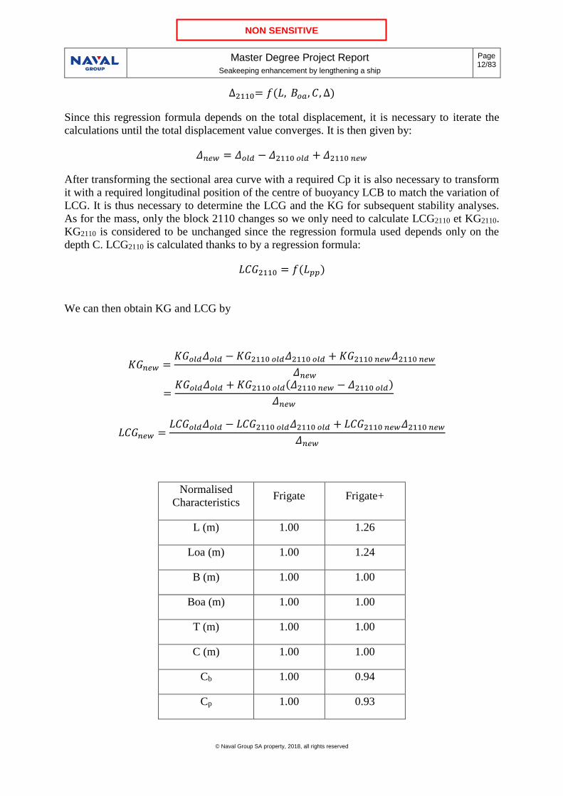
Normalised
Characteristics Frigate Frigate+
L (m) 1.00 1.26
Loa (m) 1.00 1.24
B (m) 1.00 1.00
Boa (m) 1.00 1.00
T (m) 1.00 1.00
C (m) 1.00 1.00
Cb 1.00 0.94
Cp 1.00 0.93

Master Degree Project Report
Seakeeping enhancement by lengthening a ship
Page 13/83
© Naval Group SA property, 2018, all rights reserved
NON SENSITIVE
Normalised
Characteristics Frigate Frigate+
∆2110 (t) 1.00 1.67
KG2110 (m) 1.00 1.00
LCG2110 (m) 1.00 1.29
∆ (t) 1.00 1.18
KG (m) 1.00 0.98
LCG (m) 1.00 1.11
Table 1: Reference frigate and lengthened frigate normalised main characteristics
3.3 Sectional area curve transformation
An Excel VBA (Visual Basic for Applications, the Excel programming language) software
routine has been developed in order to obtain the Frigate+ sectional area curve using Lackenby’s
method (Reference [3]). The routine main input data are the reference frigate sectional area curve
coordinates; its main output data are the modified sectional area curve coordinates in a “.txt” file.
3.3.1 Transformation by variation of the prismatic coefficient
This transformation, only applicable for ships without a parallel middle body, is detailed in
Reference [3]. (Reference [3]). It comprises the following three steps:
The first: split and normalization of the sectional area curve
The second: adjustment of the sectional area curve
The third: setting back to scale of the sectional area curve
The validation of this method is provided in Lackenby’s publication.
Step 1
First of all, the sectional area curve is split into two parts: from x = 0 to amidships and from
amidships to x = L. For each of these two halves, the y coordinates are divided by the midship
section underwater area Am so that the y coordinates for each half vary from 0 to 1. The x
coordinates are divided by the length corresponding to each half so that the x coordinates for
each half vary between 0 and 1.
So we have the following transformations:
For x aft of the midship section: 𝑥1 =𝑥
𝐿𝑎𝑓𝑡
Master Degree Project Report
Seakeeping enhancement by lengthening a ship
Page 14/83
© Naval Group SA property, 2018, all rights reserved
NON SENSITIVE
For x forward of the midship section: 𝑥1 =𝑥−𝐿𝑎𝑓𝑡
𝐿𝑓𝑜𝑟
For all x: 𝑦1 =𝑦
𝐴𝑚
With:
- Laft = length of the first part of the sectional area curve (which corresponds to the
longitudinal position of the amidships section)
- Lfor = length of the second one (Lfor + Laft = L).
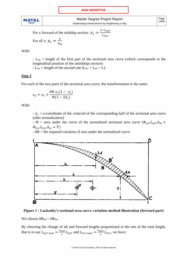
Step 2
For each of the two parts of the sectional area curve, the transformation is the same:
𝑥2 = 𝑥1 +𝛿𝛷 𝑥1(1 − 𝑥1)
𝛷(1 − 2�̅�1)
With:
- �̅�1 = x-coordinate of the centroid of the corresponding half of the sectional area curve
(after normalization)
- Φ = area under the curve of the normalized sectional area curve (𝛷𝑎𝑓𝑡𝐿𝑎𝑓𝑡𝐴𝑚 +
𝛷𝑓𝑜𝑟𝐿𝑓𝑜𝑟𝐴𝑚 = 𝛻)
- δΦ = the required variation of area under the normalized curve.
Figure 1 : Lackenby's sectional area curve variation method illustration (forward part)
We choose δΦaft = δΦfor.
By choosing the change of aft and forward lengths proportional to the one of the total length,
that is to say 𝐿𝑎𝑓𝑡 𝑛𝑒𝑤 =𝐿𝑛𝑒𝑤
𝐿𝐿𝑎𝑓𝑡 and 𝐿𝑓𝑜𝑟 𝑛𝑒𝑤 =
𝐿𝑛𝑒𝑤
𝐿𝐿𝑓𝑜𝑟, we have:

Master Degree Project Report
Seakeeping enhancement by lengthening a ship
Page 15/83
© Naval Group SA property, 2018, all rights reserved
NON SENSITIVE
𝐶𝑝 𝑛𝑒𝑤 =∇𝑛𝑒𝑤
𝐴𝑚 𝑛𝑒𝑤𝐿𝑛𝑒𝑤
=1
𝐴𝑚 𝑛𝑒𝑤𝐿𝑛𝑒𝑤(𝛷𝑎𝑓𝑡 𝑛𝑒𝑤𝐿𝑎𝑓𝑡 𝑛𝑒𝑤𝐴𝑚 𝑛𝑒𝑤 + 𝛷𝑓𝑜𝑟 𝑛𝑒𝑤𝐿𝑓𝑜𝑟 𝑛𝑒𝑤𝐴𝑚 𝑛𝑒𝑤)
=1
𝐿((𝛷𝑎𝑓𝑡 + 𝛿𝛷)𝐿𝑎𝑓𝑡 + (𝛷𝑓𝑜𝑟 + 𝛿𝛷)𝐿𝑓𝑜𝑟)
=1
𝐿(𝛷𝑎𝑓𝑡𝐿𝑎𝑓𝑡 + 𝛷𝑓𝑜𝑟𝐿𝑓𝑜𝑟) + 𝛿𝛷
= 𝐶𝑝 + 𝛿𝛷
So we choose δΦaft = δΦfor = δCp.
It is to be noted that for a δCp > 0, we have, as expected, an increase in the area under the curve
forward of the amidships section as shown in Figure 1. It also occurs aft of the amidships section.
Indeed, aft we have 𝑥2 − 𝑥1 = 𝛿𝑥 < 0 since (1 − 2�̅�1 𝑎𝑓𝑡) < 0 whereas (1 − 2�̅�1 𝑓𝑜𝑟) > 0.
Step 3
The sectional area curve is put back to scale by the following operations:
For x aft of the midship section: 𝑥3 = 𝑥2𝐿𝑎𝑓𝑡 𝑛𝑒𝑤
For x forward of the midship section: 𝑥3 = 𝑥2𝐿𝑓𝑜𝑟 𝑛𝑒𝑤 + 𝐿𝑎𝑓𝑡 𝑛𝑒𝑤
For all x: 𝑦3 = 𝑦2𝐴𝑚 𝑛𝑒𝑤 (= 𝑦2𝐴𝑚 in our case)
Figure 2: Illustration of the sectional area curve transformation by Cp variation

Master Degree Project Report
Seakeeping enhancement by lengthening a ship
Page 16/83
© Naval Group SA property, 2018, all rights reserved
NON SENSITIVE
Figure 3: Excel tool for sectional area curve transformation by Cp variation
Figure 3 shows the Excel tool I coded to use this sectional area curve transformation. There are
four command buttons on this sheet:
• “Clear Excel Sheet” deletes the curves coordinates, the plot and the input parameters. It
clears all data but the layout of the sheet is retained.
• “Import sectional area curve” is used to import the old sectional area curve (on the left)
from a text file.
• “Calculate new sectional area curve” is used to calculate the coordinates of the new
sectional area curve. The input data for this calculation are the reference ship sectional
area curve coordinates and the Cp variation required. The red parameters (Cp variation)
are mandatory whilst the blue ones (new length, new midship section area) are not as
they are set to a default value. The new sectional area curve coordinates are displayed to
the right of the screen and both the old and the new sectional area curves are shown on
the same graph.
• “Export new sectional area curve” is used to export the new sectional area curve
coordinates to a text file.
3.3.2 Transformation by variation of the centre of buoyancy
This transformation is necessary to adjust the variation of the LCB compared to the variation of
Frigate+ LCG. The LCG is determined by a regression formula and the variation of LCB is
obtained by the transformation of the sectional area curve to meet the new prismatic coefficient.
This transformation, called « swinging » of the sectional area curve is:
𝑥𝑛𝑒𝑤 = 𝑥 + 𝛿𝑥 = 𝑥 + 𝑦 tan𝜃
Where:

Master Degree Project Report
Seakeeping enhancement by lengthening a ship
Page 17/83
© Naval Group SA property, 2018, all rights reserved
NON SENSITIVE
- y is y coordinate of the sectional area curve
- tan 𝜃 =𝛿𝐿𝐶𝐵
�̅�
- �̅� is the y coordinate of the centroid of the sectional area curve
θ corresponds to the sweeping of angle of each point going from x to x à xnew (see Figure 4).
Figure 4 : Sectional area curve swinging illustration
The proof of this method is not provided in Reference [3]; one is thus proposed in Appendix 1.
Figure 5: Illustration of the sectional area curve transformation by LCB variation

Master Degree Project Report
Seakeeping enhancement by lengthening a ship
Page 18/83
© Naval Group SA property, 2018, all rights reserved
NON SENSITIVE
Figure 6: Excel tool for sectional area curve transformation by LCB variation
Figure 6 shows the Excel tool I coded to use this sectional area curve transformation. It is
identical to the tool for the Cp variation transformation.
This method has the property of conserving the amidships section area (it only induces a δx), the
length (δx null for x = 0 and x = L) and the displacement. Since these three characteristics are
unchanged, so is the prismatic coefficient.
This transformation does not interfere with the previous one. However, the order in which the
two transformations are applied is important. If this transformation was first applied and the
transformation related to the variation of Cp applied in second, then:
- The resulting Cp would be the one required since the transformation related to the LCB
does not affect Cp.
- The resulting LCB would not be, however, the one required as the Cp variation related
transformation also leads to a change in LCB.
3.4 Hull form transformations
Once the new sectional area curve has been obtained by application of Lackenby’s method, the
reference hull form shape needs to be modified so that its sectional area curve corresponds to
this new sectional area curve. This can be done by modifying the cross sections representing the
hull. These cross sections are defined by their shapes and by their longitudinal positions. There
are thus two possible choices:
- Modifying the sections shapes
- Modifying the sections positions

Master Degree Project Report
Seakeeping enhancement by lengthening a ship
Page 19/83
© Naval Group SA property, 2018, all rights reserved
NON SENSITIVE
A possible third choice would be modifying both at the same time but we would have to choose
which relative weight to give to the modification of the cross section shapes compared to the
modification of positions. Moreover, that would make two transformations instead of one and
there does not seem to be real value to it in our case so this method has not been studied.
3.4.1 Modification of cross section shapes
It is the first method that has been studied since a study on this transformation had already been
undertaken at Naval Group by Benoît Quesson (Reference [2]) in 2104. Improvements of this
method has been made in this study in order to:
- Enhance the accuracy of the new cross sectional shapes obtained by the calculations
- Ensure that there are no restrictions to the possible cross sectional shapes
- And, most of all, ensure that the required shape is correctly generated (e.g. no
discontinuity or local aberrations)
The idea behind this deformation is to make it so that the underwater part of the new section is
a transformation of only the underwater part of the old section and, similarly, that the above
water part of the new section is a transformation of only the above water part of the old section.
So this method takes as input a reference section with its draught and depth, a new waterline
breadth, a new overall breadth, a new draught, a new depth and a new underwater area and gives
as output the new section.
This transformation of a section consists in a multiplication of the two parts (underwater and
above water) of the old section by a polynomial in z of degree 2 for the underwater part and
degree 1 for the above water part and in an adjustment of the z coordinates related to the new
values Tnew et Cnew. This can be written:
• For z ≤ T : 𝐵𝑛𝑒𝑤(𝑧𝑛𝑒𝑤) = 𝐵(𝑧)(𝑐1𝑧𝑛𝑒𝑤2 + 𝑐2𝑧𝑛𝑒𝑤 + 𝑐3)
• For z ≥ T : 𝐵𝑛𝑒𝑤(𝑧𝑛𝑒𝑤) = 𝐵(𝑧)(𝑎𝑧𝑛𝑒𝑤 + 𝑏)
The three conditions used to determine c1, c2 and c3 are related to the function 𝐵𝑛𝑒𝑤(𝑧𝑛𝑒𝑤) while
𝑧𝑛𝑒𝑤 varies between 0 and 𝑇𝑛𝑒𝑤. They are:
1. Underwater area of the new section equals the required area (improvement of existing
work)
2. Continuity in znew = Tnew of the new section that is to say no discontinuity in the hull
(condition already used in existing work)
3. Continuity in znew = Tnew of the slope of the new section that is to say no hard chine in the
hull (improvement of existing work)
The two conditions used to determine a and b are:
1. Waterline breadth satisfied: 𝐵𝑛𝑒𝑤(𝑇𝑛𝑒𝑤) = 𝐵𝑛𝑒𝑤
2. Overall breadth satisfied: 𝐵𝑛𝑒𝑤(𝐶𝑛𝑒𝑤) = 𝐵𝑜𝑎 𝑛𝑒𝑤
For this method, the overall breadth Boa refers to the breadth at a height equal to the depth of the
ship.

Master Degree Project Report
Seakeeping enhancement by lengthening a ship
Page 20/83
© Naval Group SA property, 2018, all rights reserved
NON SENSITIVE
Figure 7 : Illustration of a section transformation
The complete calculations and equations regarding this transformation are detailed in Appendix
2.
Figure 8 : Excel tool for section transformation
Figure 8 shows the Excel tool I coded to use this section transformation. It is similar to the tools
for the sectional area curve transformations except that there is an additional import command
button. Indeed, this transformation requires not only the old section coordinates but the new
sectional area required which is calculated here by interpolation using the new sectional area
curve coordinates (which is imported with the additional import command button). Modification
of the cross section longitudinal positions
Master Degree Project Report
Seakeeping enhancement by lengthening a ship
Page 21/83
© Naval Group SA property, 2018, all rights reserved
NON SENSITIVE
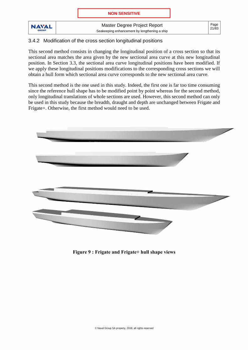
3.4.2 Modification of the cross section longitudinal positions
This second method consists in changing the longitudinal position of a cross section so that its
sectional area matches the area given by the new sectional area curve at this new longitudinal
position. In Section 3.3, the sectional area curve longitudinal positions have been modified. If
we apply these longitudinal positions modifications to the corresponding cross sections we will
obtain a hull form which sectional area curve corresponds to the new sectional area curve.
This second method is the one used in this study. Indeed, the first one is far too time consuming
since the reference hull shape has to be modified point by point whereas for the second method,
only longitudinal translations of whole sections are used. However, this second method can only
be used in this study because the breadth, draught and depth are unchanged between Frigate and
Frigate+. Otherwise, the first method would need to be used.
Figure 9 : Frigate and Frigate+ hull shape views
Master Degree Project Report
Seakeeping enhancement by lengthening a ship
Page 22/83
© Naval Group SA property, 2018, all rights reserved
NON SENSITIVE
3.5 Structure
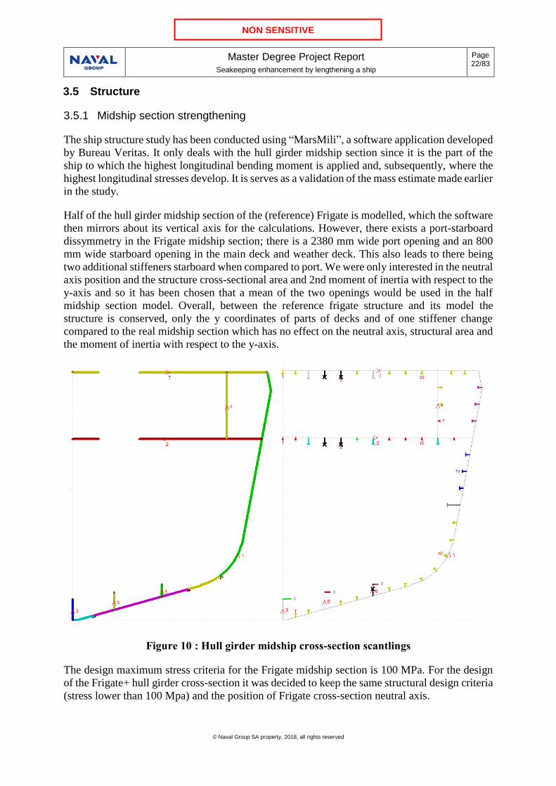
3.5.1 Midship section strengthening
The ship structure study has been conducted using “MarsMili”, a software application developed
by Bureau Veritas. It only deals with the hull girder midship section since it is the part of the
ship to which the highest longitudinal bending moment is applied and, subsequently, where the
highest longitudinal stresses develop. It is serves as a validation of the mass estimate made earlier
in the study.
Half of the hull girder midship section of the (reference) Frigate is modelled, which the software
then mirrors about its vertical axis for the calculations. However, there exists a port-starboard
dissymmetry in the Frigate midship section; there is a 2380 mm wide port opening and an 800
mm wide starboard opening in the main deck and weather deck. This also leads to there being
two additional stiffeners starboard when compared to port. We were only interested in the neutral
axis position and the structure cross-sectional area and 2nd moment of inertia with respect to the
y-axis and so it has been chosen that a mean of the two openings would be used in the half
midship section model. Overall, between the reference frigate structure and its model the
structure is conserved, only the y coordinates of parts of decks and of one stiffener change
compared to the real midship section which has no effect on the neutral axis, structural area and
the moment of inertia with respect to the y-axis.
Figure 10 : Hull girder midship cross-section scantlings
The design maximum stress criteria for the Frigate midship section is 100 MPa. For the design
of the Frigate+ hull girder cross-section it was decided to keep the same structural design criteria
(stress lower than 100 Mpa) and the position of Frigate cross-section neutral axis.

Master Degree Project Report
Seakeeping enhancement by lengthening a ship
Page 23/83
© Naval Group SA property, 2018, all rights reserved
NON SENSITIVE
The bending moment is calculated with the formula:
𝑀𝑓 =𝛥 𝐿𝑜𝑎𝑔
𝑚
Where m is a coefficient computed using formulas defined in Naval Group structural calculation
manual and which is usually around 25. The moment of inertia and the resisting surface are given
by MarsMili. The stresses in the lowest part and the highest part of the section are then given by:
𝜎𝑙𝑝 =𝑀𝑓𝐼𝐷
𝜎ℎ𝑝 =𝑀𝑓𝐼(𝐶 − 𝐷)
Where:
- 𝜎𝑙𝑝 is the stress in the lowest part
- 𝜎ℎ𝑝 is the stress in the highest part
- C is the depth of the ship
- D is the height of the neutral axis.
It was also decided to only change the thickness of the plates to strengthen the midship section
and to keep the stiffeners unchanged.
Table 2 shows the different structural data for Frigate and Frigate+ (Designed Frigate, i.e not the
actual Frigate but its design stage, has a displacement lower than the actual Frigate that is why
the displacement is 0.936 and not 1).
Designed Frigate Frigate+
Displacement used for the bending
moment calculation Δ (t) 0.936 1.136
Bending moment / g (t.m) 0.936 1.404
Midship section structure cross
section area S (m2) 1 1.576
Neutral axis height D (m) 1 1.003
Transverse moment of inertia with
respect to the neutral axis I (m4) 1 1.496
Stress in lowest part (MPa) 1 1.005
Table 2 : Midship section normalised structural data

Master Degree Project Report
Seakeeping enhancement by lengthening a ship
Page 24/83
© Naval Group SA property, 2018, all rights reserved
NON SENSITIVE
3.5.2 Displacement estimate
This structural strengthening due the increase in length and displacement (estimated with a
regression formula at the beginning of study, as explained in Section 3.2) can then be used to
calculate the new displacement (design iteration). If this new displacement calculation is
different from the one previously used to calculate the bending moment then an iteration on the
structural strengthening is necessary with this new displacement as a basis for the bending
moment calculation.
It is estimated that the increase in mass due to strengthening is proportional to the increase in
midship section structure cross section area. The ratio of the new structure mass over the old one
is then taken as the ratio of the new midship section structure cross section area over the old one.
If we consider the structure strengthening over the whole length of the ship then:
𝛥𝑛𝑒𝑤 = (𝛥 − 𝛥2110) + 𝛥2110𝐿𝑜𝑎 𝑛𝑒𝑤𝐿𝑜𝑎
𝑆𝑛𝑒𝑤𝑆
However, only the longitudinal structural members have been reinforced since they are the only
ones modelled in our MarsMili midship section. Their overall weight approximately amounts to
70 % of Weight Group 2110 which leads to the following modified formula:
𝛥𝑛𝑒𝑤 = (𝛥 − 𝛥2110) + 𝛥2110𝐿𝑜𝑎 𝑛𝑒𝑤𝐿𝑜𝑎
(0.3 + 0.7𝑆𝑛𝑒𝑤𝑆)
Nevertheless, this is still an overestimation because the ship structure is not strengthened over
its entire length as much as in the amidships area where the bending moment is maximal. At the
fore and aft ends, for instance, longitudinal strength is not the critical structural criteria and the
structure does not require strengthening. A coefficient lower than 1 needs to be added before 𝑆𝑛𝑒𝑤
𝑆 leading to the final formula:
𝛥𝑛𝑒𝑤 = (𝛥 − 𝛥2110) + 𝛥2110𝐿𝑜𝑎 𝑛𝑒𝑤𝐿𝑜𝑎
(0.3 + 0.7 (𝛼𝑆𝑛𝑒𝑤𝑆+ 1 − 𝛼))
This coefficient α corresponds to an equivalent percentage of the ship length which is reinforced
as much as the midship section. This coefficient has been calculated to be 0.47 for Frigate. This
calculation is detailed in Appendix 3.
The new displacement is obtained by applying this formula. If necessary, an iteration on the
structure strengthening is done until the input and output displacements converge (here a 1%
maximal difference is chosen).

Master Degree Project Report
Seakeeping enhancement by lengthening a ship
Page 25/83
© Naval Group SA property, 2018, all rights reserved
NON SENSITIVE
Frigate Frigate+
Displacement at the beginning of study (t) 1 1.177
Displacement after 1st strengthening of
structure (t)
- 1.136
Number of additional iterations necessary for
a 1 % convergence
- 1
Displacement after iterations (t) - 1.129
Convergence of the last iteration: difference
between last and second last iteration (%)
- 0.56
Table 3 : Frigate+ normalised displacement estimate

Master Degree Project Report
Seakeeping enhancement by lengthening a ship
Page 26/83
© Naval Group SA property, 2018, all rights reserved
NON SENSITIVE
4 Seakeeping and Operability
The seakeeping software used is Precal_R (Reference [17]), developed within the Cooperative
Research Ships (CRS) framework. It uses the frequency domain linear 3D diffraction theory and
can be used to calculate the motion response in regular waves at arbitrary speed and heading.
RAOs (Response Amplitude Operator) and RMS (Root Mean Square) of ship motions can be
given as output.
For each combination of ship speed, wave direction and wave frequency the ship-wave
interaction is described as the superposition of the forces on a fixed ship in incoming waves (the
diffraction part) and the forces on an oscillating ship in calm water (the radiation part).
The wave excitation forces are composed of the incoming wave forces and the diffraction wave
forces which are obtained by integration of the corresponding pressures over the hull surface. In
the same way, the reaction forces are expressed in terms of added mass and damping coefficients.
The assumption of linearity implies that in principle the results are valid for small wave
amplitudes and small motion amplitudes only.
4.1 Precal_R seakeeping results
The hull shapes used for the seakeeping calculations are bare hulls without appendices such as
roll stabilising fins or bilge keel. The linear equivalent roll damping coefficient 𝐵𝑒𝑞𝑣 is taken to
be a percentage 𝛿 of the critical roll damping coefficient 𝐵𝑐𝑟𝑖𝑡 (see Figure 11).
𝐵𝑒𝑞𝑣 = 𝛿 𝐵𝑐𝑟𝑖𝑡
𝐵𝑐𝑟𝑖𝑡 = 2√(𝑀44 + 𝐴44(𝑛𝑎𝑡)
)𝐶44
Where:
- 𝑀44 is the roll moment of inertia
- 𝐴44(𝑛𝑎𝑡)
is the roll-roll added mass coefficient at the roll natural frequency
- 𝐶44 is the roll restoring coefficient.
Precal_R makes this percentage (also called damping ratio) vary with the ship speed:
𝛿 = 𝛿0(1 + 0.8(1 − 𝑒−10 𝐹𝑛))
𝛿0is the input parameter, it has been chosen as 10 % (value usually used by Naval Group
hydrodynamics specialists).

Master Degree Project Report
Seakeeping enhancement by lengthening a ship
Page 27/83
© Naval Group SA property, 2018, all rights reserved
NON SENSITIVE
Figure 11 : Roll damping ratio as a function of the Froude number
4.1.1 Transfer functions
Only the heave, roll and pitch transfer functions are plotted here because heave and pitch, cause
slamming, which we want to reduce, and roll is usually found to be critical for compliance with
warship operating criteria. These transfer functions are plotted for different speeds but only for
a unique wave heading corresponding to the most critical situation. So, the heave and pitch
transfer functions are plotted for a wave relative (compared to the ship forward direction)
heading of 180° and the roll transfer functions are plotted for a wave relative heading of 90°.
Figure 12 : Frigate heave transfer function for a 180° wave heading
0.08
0.1
0.12
0.14
0.16
0.18
0.2
0 0.1 0.2 0.3 0.4 0.5 0.6
Ro
ll d
amp
ing
rati
o
Froude number
0
0.2
0.4
0.6
0.8
1
1.2
1.4
1.6
0 5 10 15 20 25 30 35
He
ave
(m
.m-1
)
Wave period (s)
Frigate
V=0
V=10
V=15
V=20
V=25
V=30
Master Degree Project Report
Seakeeping enhancement by lengthening a ship
Page 28/83
© Naval Group SA property, 2018, all rights reserved
NON SENSITIVE
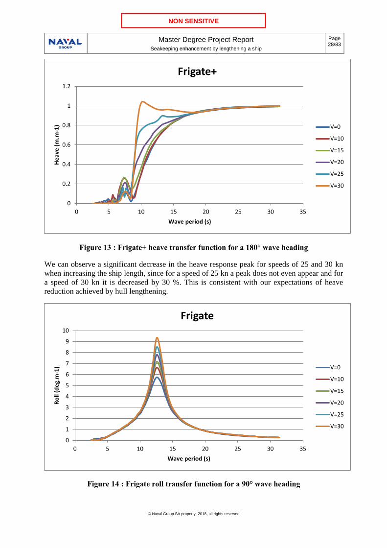
Figure 13 : Frigate+ heave transfer function for a 180° wave heading
We can observe a significant decrease in the heave response peak for speeds of 25 and 30 kn
when increasing the ship length, since for a speed of 25 kn a peak does not even appear and for
a speed of 30 kn it is decreased by 30 %. This is consistent with our expectations of heave
reduction achieved by hull lengthening.
Figure 14 : Frigate roll transfer function for a 90° wave heading
0
0.2
0.4
0.6
0.8
1
1.2
0 5 10 15 20 25 30 35
He
ave
(m
.m-1
)
Wave period (s)
Frigate+
V=0
V=10
V=15
V=20
V=25
V=30
0
1
2
3
4
5
6
7
8
9
10
0 5 10 15 20 25 30 35
Ro
ll (d
eg.
m-1
)
Wave period (s)
Frigate
V=0
V=10
V=15
V=20
V=25
V=30

Master Degree Project Report
Seakeeping enhancement by lengthening a ship
Page 29/83
© Naval Group SA property, 2018, all rights reserved
NON SENSITIVE
Figure 15 : Frigate+ roll transfer function for a 90° wave heading
For roll we can see that Frigate+ peak responses at all speeds are much higher than those of
Frigate. They increase significantly with increasing ship speeds. Indeed, for a speed of 0 kn the
increase is of the order of 20 % and for a speed of 30 kn it is approximately 80 %.
No explanation for these incoherent results has been found by Naval Group hydrodynamics
specialists based in Lorient. Consequently, the operability comparison presented in following
sections of this report use the Frigate roll results for Frigate+ to measure the heave and pitch
variation influence on the operability (not perturbated by this puzzling roll results).
0
2
4
6
8
10
12
14
16
18
0 5 10 15 20 25 30 35
Ro
ll (d
eg.
m-1
)
Wave period (s)
Frigate+
V=0
V=10
V=15
V=20
V=25
V=30

Master Degree Project Report
Seakeeping enhancement by lengthening a ship
Page 30/83
© Naval Group SA property, 2018, all rights reserved
NON SENSITIVE
Figure 16 : Frigate pitch transfer function for a 180° wave heading
Figure 17 : Frigate+ pitch transfer function for a 180° wave heading
We can see a decrease in the pitch response peak at all speeds. This decrease varies between 10
and 12 % throughout the speed range considered except at 30 kn for which it varies by 17 %.
This pitch reduction, like the heave reduction, is consistent with our expectations.
0
0.5
1
1.5
2
2.5
3
0 5 10 15 20 25 30 35
Pit
ch (
de
g.m
-1)
Wave period (s)
Frigate
V=0
V=10
V=15
V=20
V=25
V=30
0
0.5
1
1.5
2
2.5
0 5 10 15 20 25 30 35
Pit
ch (
de
g.m
-1)
Wave period (s)
Frigate+
V=0
V=10
V=15
V=20
V=25
V=30

Master Degree Project Report
Seakeeping enhancement by lengthening a ship
Page 31/83
© Naval Group SA property, 2018, all rights reserved
NON SENSITIVE
4.1.2 Pitch
Pitch is the ship motion we are especially interested in as it is highly dependent of the length of
a ship. The transfer functions for the most critical case (180° wave heading) have already been
presented in Section 4.1.1. This section presents Frigate+ pitch RMS values as percentages of
those of Frigate for 3 speeds (0 kn, 15 kn usual operational speed and 30 kn possible maximum
speed) for 3 sea states: sea state 4/5 (Figure 18), sea state 5 (Figure 19) and sea state 5/6 (Figure
20).
We can see a decrease in the RMS value for Frigate+ at all speeds, wave headings and sea states.
The normalised pitch RMS at 90° and 270° wave headings have been set at 100 % in order to
avoid representing the “freak” normalised pitch RMS results calculated at these values which
distort the overall illustration of the results. Factually, at these wave headings, pitch is almost
zero but the variation in percentage between the RMS calculated for Frigate and Frigate+ can be
extremely important compared to those for other wave headings. For instance, for sea state 4/5,
90° wave heading and 15 kn speed, the RMS value for Frigate is 0.021 °/m and 0.078 °/m for
Frigate+ which corresponds to 367 % of Frigate RMS value. As Frigate+ RMS is between 60
and 100 % of Frigate RMS for the other headings, having a value of 367% in the graph “hides”
the other results due to the change of scale necessary to plot the 367% value.
Figure 18 : Frigate+ pitch RMS as percentage of Frigate pitch RMS for sea state 4/5

Master Degree Project Report
Seakeeping enhancement by lengthening a ship
Page 32/83
© Naval Group SA property, 2018, all rights reserved
NON SENSITIVE
Figure 19 : Frigate+ pitch RMS as percentage of Frigate pitch RMS for sea state 5
Figure 20 : Frigate+ pitch RMS as percentage of Frigate pitch RMS for sea state 5/6

Master Degree Project Report
Seakeeping enhancement by lengthening a ship
Page 33/83
© Naval Group SA property, 2018, all rights reserved
NON SENSITIVE
We can see a 20 to 24 % (depending on the speed) decrease for head seas at sea state 4/5, a 15
to 18 % decrease at sea state 5 and a 7 to 12 % decrease at sea state 5/6. This relative decrease
diminishes as the sea state increases. To confirm this trend, calculations have been undertaken
at higher and lower sea states. The results, are presented in Figures 20, 21 and 22. For an easier
reading of the graphs, one graph corresponds to only one speed. Below are the 0, 15 and 30 kn
results and, as previously, the 90° (and 270°) results have been set at 100 %.
Figure 21 : Frigate+ pitch RMS as percentage of Frigate pitch RMS for V = 0 kn and for
different sea states
50
60
70
80
90
100
110180
165
150
135
120
105
90
75
60
45
30
150
345
330
315
300
285
270
255
240
225
210
195
V = 0 knSS 2
SS 3
SS 4
SS 4/5
SS 5
SS 5/6
SS 6
SS 7
SS 8

Master Degree Project Report
Seakeeping enhancement by lengthening a ship
Page 34/83
© Naval Group SA property, 2018, all rights reserved
NON SENSITIVE
Figure 22 : Frigate+ pitch RMS as percentage of Frigate pitch RMS for V = 15 kn and for
different sea states
Figure 23 : Frigate+ pitch RMS as percentage of Frigate pitch RMS for V = 30 kn and for
different sea states
These results confirm that the higher the sea state is, the lesser is the relative (%) pitch reduction
achieved by lengthening the ship. For head seas, for a speed of 0 kn, the decrease in pitch is 33%
for sea states 2 and 3 and only 5% for sea states 7 and 8. There also appears to be a convergence
50
60
70
80
90
100
110180
165150
135
120
105
90
75
60
45
3015
0345
330
315
300
285
270
255
240
225
210195
V = 15 kn
SS2
SS 3
SS 4
SS 4/5
SS 5
SS 5/6
SS 6
SS 7
SS 8

Master Degree Project Report
Seakeeping enhancement by lengthening a ship
Page 35/83
© Naval Group SA property, 2018, all rights reserved
NON SENSITIVE
toward this 5 % value when the sea state increases. For a speed of 30 kn, the decrease varies
between 33 % and 1 % depending on the sea state.
Precal_R output includes RAOs (Response Amplitude Operator) and RMS (Root Mean Square)
from which it is possible to plot graphs such as the ones above. However, it does not include
operability assessments based on the seakeeping characteristics of a ships against a set of limiting
seakeeping criteria (motions/velocities/accelerations) such as those defined in Reference [5] for
naval ships.
Moreover, Precal_R does not provide RAO and RMS for relative vertical motions, velocities and
accelerations nor does it calculate Motion Sickness Incidence (MSI), Motion Induced
Interruption (MII) and Lateral Force Estimator (LFE).
Thus, the development of a tool for postprocessing Precal_R RAOs in order to calculate
slamming and emergence, MSI, MII and LFE as long as operability graphs was needed. This
tool is an Excel VBA routine.
4.2 Calculations et Formulas used in Precal_R output data post processing
4.2.1 Wave spectrum
The wave spectrum chosen for this study is the JONSWAP (Joint North Sea Wave Project) wave
spectrum which is defined as follows (Reference [17]):
𝑆(𝜔) =𝛼𝑔2
𝜔5𝑒𝑥𝑝 (−
𝛽𝜔𝑝4
𝜔4) 𝛾𝑎
Where:
• g is the gravitational acceleration 9.81 m.s-2
• ω is the (angular) frequency
• 𝛽 =5
4
• 𝜔𝑝 is the spectrum peak frequency
• 𝛾 = 3.3
• 𝑎 = 𝑒𝑥𝑝 (−(𝜔−𝜔𝑝)
2
2𝜔𝑝2𝜎2
)
• 𝜎 = { 0.07 𝑖𝑓 𝜔 ≤ 𝜔𝑝
0.09 𝑖𝑓 𝜔 > 𝜔𝑝
• α is so that 16∫ 𝑆(𝜔)𝑑𝜔 = 𝐻2+∞
0
• H is the significant wave height

Master Degree Project Report
Seakeeping enhancement by lengthening a ship
Page 36/83
© Naval Group SA property, 2018, all rights reserved
NON SENSITIVE
With this spectrum and the RAO transfer functions we can calculate the RMS (Root Mean
Square) of this motion and check if it meets a criteria (most criteria are expressed in RMS).
𝜎 = √∫ |𝑅𝐴𝑂(𝜔)|2𝑆(𝜔)𝑑𝜔+∞
0
The sea states concerned by this study are sea states 4/5, 5 and 5/6 which significant wave heights
and peak periods, defined in accordance with the values specified in Reference [4], are given in
the table below.
Sea State H (m) T (s)
2 0.3 7.5
3 0.88 7.5
4 1.88 8.8
4/5 2.5 9.2
5 3.25 9.7
5/6 4 11
6 5 12.4
7 7.5 15
8 11.5 16.4
Table 4 : Sea states significant wave heights and peak periods
The JONSWAP wave spectra for sea states 4/5, 5 and 5/6 are plotted in Figure 23Erreur !
Source du renvoi introuvable.. These are the spectra used for this study.

Master Degree Project Report
Seakeeping enhancement by lengthening a ship
Page 37/83
© Naval Group SA property, 2018, all rights reserved
NON SENSITIVE
Figure 24 : JONSWAP wave spectrum
4.2.2 Motions and derivatives
The 6 motions of a ship, i.e. surge, sway, heave, roll, pitch and yaw, respectively 𝜂1, 𝜂2, 𝜂3, 𝜂4,
𝜂5 and 𝜂6 in the following motion transfer functions, are calculated at its centre of gravity. The
motions at a given point (longitudinal, lateral and vertical motions 𝐷1, 𝐷2 and 𝐷3) are then
calculated from the ship motions and the position of the given point (the 3 rotations are the same).
These motions transfer functions are given by:
𝐷1 = 𝜂1 − (𝑋 − 𝑋𝐺)(1 − cos 𝜂6) − (𝑌 − 𝑌𝐺) sin 𝜂6 − (𝑋 − 𝑋𝐺)(1 − cos 𝜂5) + (𝑍 − 𝑍𝐺) sin 𝜂5
𝐷2 = 𝜂2 − (𝑌 − 𝑌𝐺)(1 − cos 𝜂6) + (𝑋 − 𝑋𝐺) sin 𝜂6 − (𝑌 − 𝑌𝐺)(1 − cos𝜂4) − (𝑍 − 𝑍𝐺) sin 𝜂4
𝐷3 = 𝜂3 − (𝑍 − 𝑍𝐺)(1 − cos 𝜂4) + (𝑌 − 𝑌𝐺) sin 𝜂4 − (𝑍 − 𝑍𝐺)(1 − cos 𝜂5) − (𝑋 − 𝑋𝐺) sin 𝜂5
The rotation motions being rather small, the first order approximation in rotations can be made.
This approximation is often used, it is the case for the Precal_R software for instance.
𝐷1 ~ 𝜂1 − (𝑌 − 𝑌𝐺)𝜂6 + (𝑍 − 𝑍𝐺)𝜂5
𝐷2 ~ 𝜂2 + (𝑋 − 𝑋𝐺)𝜂6 − (𝑍 − 𝑍𝐺)𝜂4
𝐷3 ~ 𝜂3 + (𝑌 − 𝑌𝐺)𝜂4 − (𝑋 − 𝑋𝐺)𝜂5
To determine the derivatives, that is to say longitudinal, lateral and vertical velocities and
accelerations, the encounter frequency between the waves and the ship must be used.
�̇�𝑖 = −𝑖𝜔𝑒 𝐷𝑖
Master Degree Project Report
Seakeeping enhancement by lengthening a ship
Page 38/83
© Naval Group SA property, 2018, all rights reserved
NON SENSITIVE
�̈�𝑖 = −𝑖𝜔𝑒 �̇�𝑖
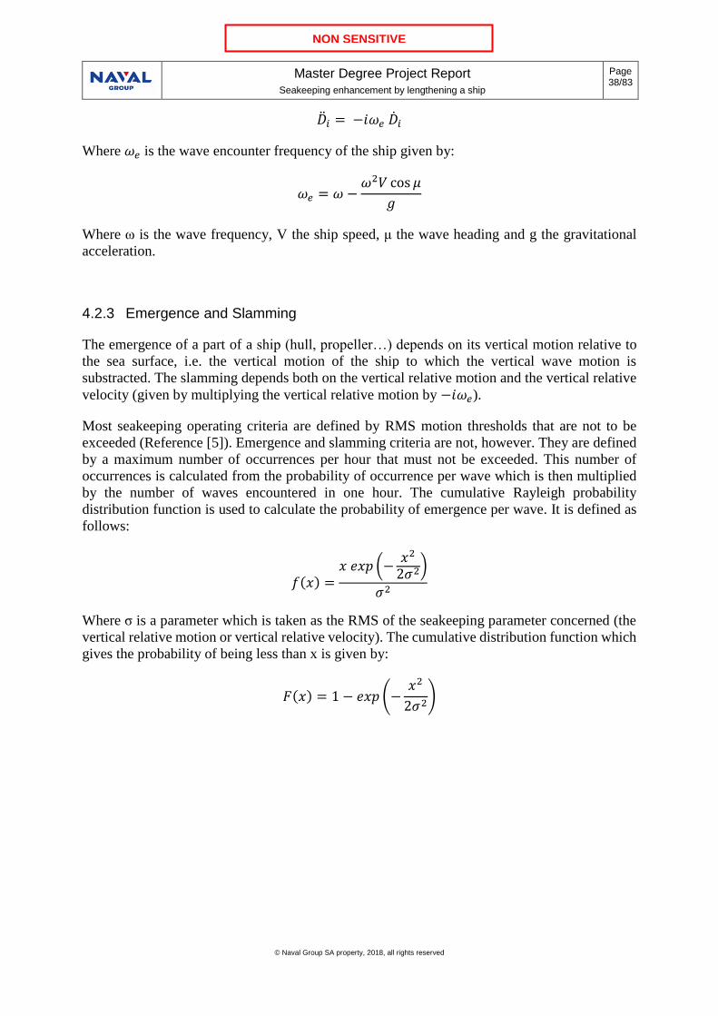
Where 𝜔𝑒 is the wave encounter frequency of the ship given by:
𝜔𝑒 = 𝜔 −𝜔2𝑉 cos 𝜇
𝑔
Where ω is the wave frequency, V the ship speed, μ the wave heading and g the gravitational
acceleration.
4.2.3 Emergence and Slamming
The emergence of a part of a ship (hull, propeller…) depends on its vertical motion relative to
the sea surface, i.e. the vertical motion of the ship to which the vertical wave motion is
substracted. The slamming depends both on the vertical relative motion and the vertical relative
velocity (given by multiplying the vertical relative motion by −𝑖𝜔𝑒).
Most seakeeping operating criteria are defined by RMS motion thresholds that are not to be
exceeded (Reference [5]). Emergence and slamming criteria are not, however. They are defined
by a maximum number of occurrences per hour that must not be exceeded. This number of
occurrences is calculated from the probability of occurrence per wave which is then multiplied
by the number of waves encountered in one hour. The cumulative Rayleigh probability
distribution function is used to calculate the probability of emergence per wave. It is defined as
follows:
𝑓(𝑥) =𝑥 𝑒𝑥𝑝 (−
𝑥2
2𝜎2)
𝜎2
Where σ is a parameter which is taken as the RMS of the seakeeping parameter concerned (the
vertical relative motion or vertical relative velocity). The cumulative distribution function which
gives the probability of being less than x is given by:
𝐹(𝑥) = 1 − 𝑒𝑥𝑝 (−𝑥2
2𝜎2)

Master Degree Project Report
Seakeeping enhancement by lengthening a ship
Page 39/83
© Naval Group SA property, 2018, all rights reserved
NON SENSITIVE
Figure 25 : Rayleigh probability distribution and cumulative functions
The probability of exceeding a given value 𝑥0 is then given by 𝑃(𝑥 ≥ 𝑥0) = 𝑒𝑥𝑝 (−𝑥02
2𝜎2)
For the emergence to occur at a location which vertical position is Z, the vertical relative motion
needs to exceed T-Z where T is the draught of the ship. So, the probability that Z exceeds T-Z is
multiplied by the number of waves encountered per hour to get the number of occurrences per
hour:
𝑁𝑏𝑒𝑚𝑒𝑟𝑔𝑒𝑛𝑐𝑒 = 𝑒𝑥𝑝 (−(𝑇 − 𝑍)2
2𝜎𝑣𝑒𝑟𝑡𝑖𝑐𝑎𝑙 𝑟𝑒𝑙𝑎𝑡𝑖𝑣𝑒 𝑚𝑜𝑡𝑖𝑜𝑛2 )
3600
𝑇𝑚
Where 𝑇𝑚 is the mean period of wave encountering and since it is expressed in s, the number of
waves encountered per hour is 3600
𝑇𝑚.
𝑇𝑚 = 2𝜋𝜎𝑣𝑒𝑟𝑡𝑖𝑐𝑎𝑙 𝑟𝑒𝑙𝑎𝑡𝑖𝑣𝑒 𝑚𝑜𝑡𝑖𝑜𝑛𝜎𝑣𝑒𝑟𝑡𝑖𝑐𝑎𝑙 𝑟𝑒𝑙𝑎𝑡𝑖𝑣𝑒 𝑣𝑒𝑙𝑜𝑐𝑖𝑡𝑦
Where 𝜎𝑥 is the parameter 𝑥 RMS.
Concerning slamming, in addition to emergence, the vertical relative velocity needs to exceed a
minimum value which is taken as 3.66√𝐿
158.5 which is the adaptation of the 12 feet per second
for a 520 feet long vessel threshold using Froude’s law (Reference [12]). So, the two probabilities
need to be multiplied and we get:
𝑁𝑏𝑠𝑙𝑎𝑚𝑚𝑖𝑛𝑔 = 𝑒𝑥𝑝 (−(𝑇 − 𝑍)2
2𝜎𝑣𝑒𝑟𝑡𝑖𝑐𝑎𝑙 𝑟𝑒𝑙𝑎𝑡𝑖𝑣𝑒 𝑚𝑜𝑡𝑖𝑜𝑛2 ) 𝑒𝑥𝑝
(
−
( 3.66√𝐿
158.5)
2
2𝜎𝑣𝑒𝑟𝑡𝑖𝑐𝑎𝑙 𝑟𝑒𝑙𝑎𝑡𝑖𝑣𝑒 𝑣𝑒𝑙𝑜𝑐𝑖𝑡𝑦2
)
3600
𝑇𝑚

Master Degree Project Report
Seakeeping enhancement by lengthening a ship
Page 40/83
© Naval Group SA property, 2018, all rights reserved
NON SENSITIVE
4.2.4 Motion Sickness Incidence (MSI)
The Motion Sickness Incidence index represents the peak percentage of a ship crew being
seasick. It usually occurs after four hours because after several hours the crew tends to
accommodate and the percentage of the crew affected by seasickness decreases. The MSI as a
function of the encountered frequency is given in Reference [13] by:
𝑀𝑆𝐼(𝜔𝑒) = ∫100
𝜎√2
log10 (�̅�)
−∞
𝑒𝑥𝑝 (−(𝑥 − 𝜇(𝜔𝑒))
2
2𝜎2)𝑑𝑥
Which can be re-written (Reference [15])
𝑀𝑆𝐼(𝜔𝑒) = 100 (1
2+1
2𝑒𝑟𝑓 (
log10(�̅�) − 𝜇(𝜔𝑒)
𝜎√2))
σ is a parameter which value has been empirically determined in Reference [13] and 𝜎 =0.4
√2.
�̅� refers to the mean vertical acceleration which has been normalised by 𝑔. For an acceleration
of the form 𝐴 sin𝜔𝑡 (𝐴 > 0) the mean absolute value normalised by 𝑔 equals to:
�̅� =𝐴
𝑔𝜋2
𝜇(𝜔𝑒) is given by the formula (Reference [13]):
𝜇(𝜔𝑒) = 0.654 + 3.697log10 (𝜔𝑒2𝜋) + 2.320 (log10 (
𝜔𝑒2𝜋))
2
There also exists a second formula (Reference [14] and [15]) but both formulas sensibly give the
same values of 𝜇(𝜔𝑒).
𝜇(𝜔𝑒) = −0.819 + 2.320 (log10(𝜔𝑒))2
𝑒𝑟𝑓 is the error function defined as:
𝑒𝑟𝑓(𝑥) = 2
√𝜋∫ 𝑒𝑥𝑝(−𝑢2)𝑑𝑢𝑥
0
The approximation used in this study for the error function is:
𝑒𝑟𝑓(𝑥)~ 𝑆𝑖𝑔𝑛(𝑥)√1 − 𝑒𝑥𝑝 (−4𝑥2
𝜋)

Master Degree Project Report
Seakeeping enhancement by lengthening a ship
Page 41/83
© Naval Group SA property, 2018, all rights reserved
NON SENSITIVE
It is a very satisfying approximation since the difference between the 𝑒𝑟𝑓 function and this
approximation never exceeds 0.7 % as shown in Figure 26.
Figure 26 : erf function approximation precision
This calculation of 𝑀𝑆𝐼(𝜔𝑒) gives a MSI transfer function from which we can calculate the total
MSI (Reference [14]):
𝑀𝑆𝐼 = ∫ 𝑀𝑆𝐼(𝜔𝑒)𝑆(𝜔)𝑑𝜔+∞
0
4.2.5 Motion Induced Interruptions (MII)
The MII calculation consists in calculating the risk of an operator tipping due to the ship motions
which would lead to an interruption of his activities. To evaluate the risk of tipping, we look at
the sum of moments at the operator’s feet (Reference [16]).
Figure 27 : Operator’s geometry for MII calculations

Master Degree Project Report
Seakeeping enhancement by lengthening a ship
Page 42/83
© Naval Group SA property, 2018, all rights reserved
NON SENSITIVE
The forces (in the plane (y, z)) applied to an operator are his weight, the deck reaction force and
the fictitious forces due to the ship lateral and vertical accelerations. The deck reaction force
consists of two components, each one applied to one of the operator’s feet. The one applied at
the foot at which the sum of the moments of the forces applied to the operator is calculated does
not induce any moment. The force applied to the other foot becomes null as soon as there is
tipping since the foot is not in contact with the deck any longer. This explains why the deck
reaction forces do not appear in the following calculations. The sum of moments at OL and OR
(see Figure 27) are:
∑𝑀𝑂𝐿 = 𝑚𝑔𝑙 cos 𝜂4 +𝑚𝑔ℎ sin 𝜂4 − (−𝑚�̈�2)ℎ − (−𝑚�̈�3)𝑙
∑𝑀𝑂𝑅 = −𝑚𝑔𝑙 cos 𝜂4 +𝑚𝑔ℎ sin 𝜂4 − (−𝑚�̈�2)ℎ + (−𝑚�̈�3)𝑙
There is tipping if ∑𝑀𝑂𝐿 < 0 or if ∑𝑀𝑂𝑅 > 0. Using the assumption of small angles, we get
tipping if:
−𝑔𝜂4 − �̈�2 − �̈�3𝑙
ℎ >
𝑔𝑙
ℎ
Or if
𝑔𝜂4 + �̈�2 − �̈�3𝑙
ℎ >
𝑔𝑙
ℎ
The MII are then simply given by the sum of probabilities that −𝑔𝜂4 − �̈�2 − �̈�3𝑙
ℎ exceeds
𝑔𝑙
ℎ
and that 𝑔𝜂4 + �̈�2 − �̈�3𝑙
ℎ exceeds
𝑔𝑙
ℎ . As opposed to the slamming calculations, here it is the
sum of probabilities and not the product because it is the occurrence of an event OR the other
that we are interested in and not an event AND the other. Like previously, it is the Rayleigh
probability that is used.
𝑀𝐼𝐼 = (𝑃 (−𝑔𝜂4 − �̈�2 − �̈�3𝑙
ℎ> 𝑔𝑙
ℎ) + 𝑃 (𝑔𝜂4 + �̈�2 − �̈�3
𝑙
ℎ> 𝑔𝑙
ℎ))3600
𝑇𝑚
𝑀𝐼𝐼 =
(
𝑒𝑥𝑝
(
−(𝑔𝑙ℎ)2
2𝜎−𝑔𝜂4−�̈�2−�̈�3
𝑙ℎ
2
)
+ 𝑒𝑥𝑝
(
−(𝑔𝑙ℎ)2
2𝜎𝑔𝜂4+�̈�2−�̈�3
𝑙ℎ
2
)
)
3600
𝑇𝑚
4.2.6 Lateral Force Estimator
The Lateral Force Estimator (LFE) is, as its name implies, a means to estimate the lateral forces
(by unit of mass). It takes into account the fictitious force due to the lateral motion and the lateral
component of the weight. By making the small angles assumption, we get:
𝐿𝐹𝐸 = −�̈�2 − 𝑔𝜂4

Master Degree Project Report
Seakeeping enhancement by lengthening a ship
Page 43/83
© Naval Group SA property, 2018, all rights reserved
NON SENSITIVE
The criteria associated to LFE are expressed in RMS so there is no calculation using Rayleigh
probabilities for the LFE.
4.3 PRECAL_R post processing Excel tool
The Excel VBA tool I coded is an Excel file with one main sheet, six imported data sheets and
one total operability sheet. The main sheet is shown in Figure 28. In this sheet there are:
• Two command buttons: one to import the surge, sway, heave, roll, pitch and yaw RAOs
Precal_R output files (they are stored in different sheets one for each motion) and the
other one to launch the calculations.
• One table with the list of all available operability parameters for calculations. The user
may fill in three columns. The first column is to select what parameters are to be used.
The second one is to specify the operability criteria which should be used for the selected
parameters. The third one is to select the parameters for which, in addition to a global
operability graph which is generated by default, specific operability graphs should be
produced.
• Several input parameters tables: one for the position of the centre of gravity of the ship
and the position of the point where the calculations should be made, one for the
significant wave height and peak period used for the wave spectrum and one (only used
if the user select the emergence or slamming parameters) with the waterline length and
draught of the ship.
• Additional information displayed through two tables: one with the number of wave
frequencies, wave headings and ship speeds contained in the imported RAOs and one
with significant wave height and peak periods corresponding to different sea states.
Figure 28 : Excel post processing tool main sheet

Master Degree Project Report
Seakeeping enhancement by lengthening a ship
Page 44/83
© Naval Group SA property, 2018, all rights reserved
NON SENSITIVE
Of the seven other sheets, six are used to store the RAOs for surge, sway, heave, roll, pitch and
yaw (one for each motion). Their format is similar to the original files given as output by
Precal_R see Figure 29.
Figure 29 : Excel post processing tool surge sheet
For each ship speed, for each wave heading, there are three columns of data. The first one
corresponds to the wave frequency, the second one to the RAO amplitude and the last one to the
RAO phase angle. Before each set of three columns, the ship speed and wave heading are given.
Once the RAOs have been imported and the user has filled in all that needs to be in the main
sheet, he can press the calculations command button. After this, an additional sheet is created for
each parameter the user has selected for the operability calculations (for surge, sway, heave, roll,
pitch and yaw the existing sheet is used, no additional sheet needs creating). Figure 29 is an
example of the roll sheet after calculations without the user having selected an additional
operability graph.
Master Degree Project Report
Seakeeping enhancement by lengthening a ship
Page 45/83
© Naval Group SA property, 2018, all rights reserved
NON SENSITIVE
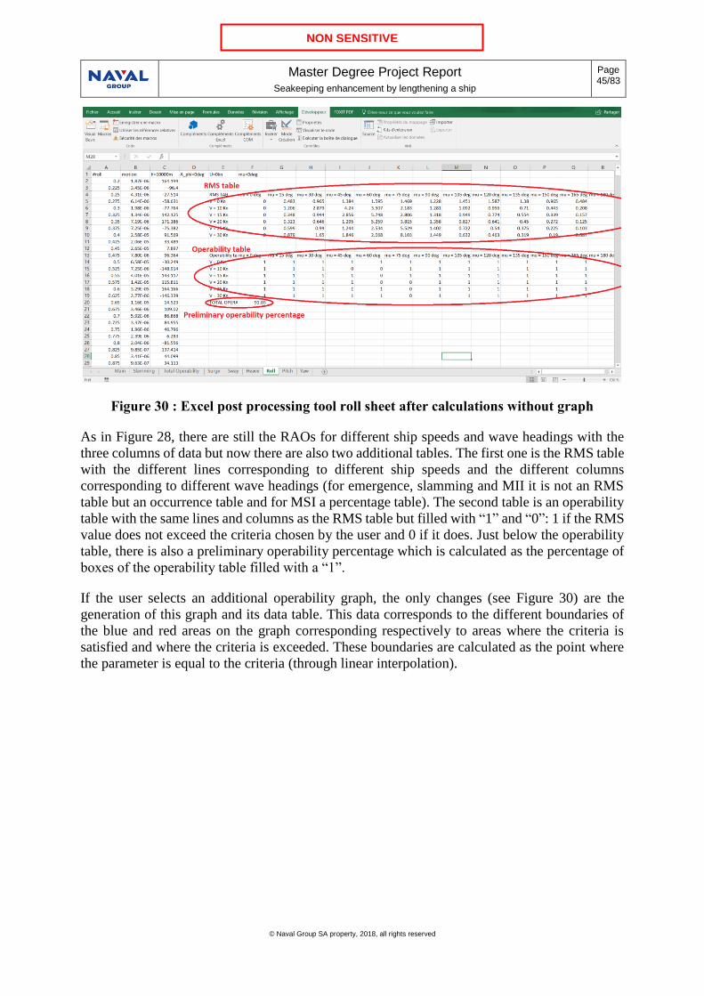
Figure 30 : Excel post processing tool roll sheet after calculations without graph
As in Figure 28, there are still the RAOs for different ship speeds and wave headings with the
three columns of data but now there are also two additional tables. The first one is the RMS table
with the different lines corresponding to different ship speeds and the different columns
corresponding to different wave headings (for emergence, slamming and MII it is not an RMS
table but an occurrence table and for MSI a percentage table). The second table is an operability
table with the same lines and columns as the RMS table but filled with “1” and “0”: 1 if the RMS
value does not exceed the criteria chosen by the user and 0 if it does. Just below the operability
table, there is also a preliminary operability percentage which is calculated as the percentage of
boxes of the operability table filled with a “1”.
If the user selects an additional operability graph, the only changes (see Figure 30) are the
generation of this graph and its data table. This data corresponds to the different boundaries of
the blue and red areas on the graph corresponding respectively to areas where the criteria is
satisfied and where the criteria is exceeded. These boundaries are calculated as the point where
the parameter is equal to the criteria (through linear interpolation).

Master Degree Project Report
Seakeeping enhancement by lengthening a ship
Page 46/83
© Naval Group SA property, 2018, all rights reserved
NON SENSITIVE
Figure 31: Excel post processing tool vertical motion sheet after calculations with graph
An example of an operability radar graph is given in Figure 31. This graph has a radial axis
corresponding to the different ship speeds and an angular axis corresponding to the different
wave headings. As previously said, blue indicates compliance with the operability criteria and
red non-compliance. In addition, the graph title provides the name of the operability criteria that
the graph represents and the ship operability percentage calculated using the boundaries of the
blue and red areas.
Figure 32 : Excel post processing tool operability graph example
0
6
12
18
24
30180
165150
135
120
105
90
75
60
45
3015
0345
330
315
300
285
270
255
240
225
210195
Vertical MotionOperability : 66 %
Master Degree Project Report
Seakeeping enhancement by lengthening a ship
Page 47/83
© Naval Group SA property, 2018, all rights reserved
NON SENSITIVE
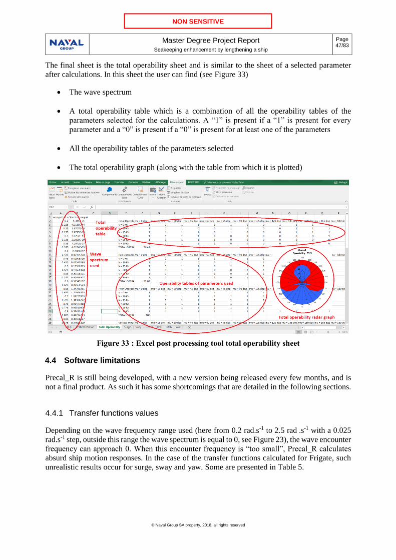
The final sheet is the total operability sheet and is similar to the sheet of a selected parameter
after calculations. In this sheet the user can find (see Figure 33)
• The wave spectrum
• A total operability table which is a combination of all the operability tables of the
parameters selected for the calculations. A “1” is present if a “1” is present for every
parameter and a “0” is present if a “0” is present for at least one of the parameters
• All the operability tables of the parameters selected
• The total operability graph (along with the table from which it is plotted)
Figure 33 : Excel post processing tool total operability sheet
4.4 Software limitations
Precal_R is still being developed, with a new version being released every few months, and is
not a final product. As such it has some shortcomings that are detailed in the following sections.
4.4.1 Transfer functions values
Depending on the wave frequency range used (here from 0.2 rad.s-1 to 2.5 rad .s-1 with a 0.025
rad.s-1 step, outside this range the wave spectrum is equal to 0, see Figure 23), the wave encounter
frequency can approach 0. When this encounter frequency is “too small”, Precal_R calculates
absurd ship motion responses. In the case of the transfer functions calculated for Frigate, such
unrealistic results occur for surge, sway and yaw. Some are presented in Table 5.

Master Degree Project Report
Seakeeping enhancement by lengthening a ship
Page 48/83
© Naval Group SA property, 2018, all rights reserved
NON SENSITIVE
Configuration # 1 2 3 4
V (kn) 10 20 25 30
µ (deg) 15 30 60 45
ω (rad/s) 1.975 1.100 1.525 0.900
ωe (rad/s) 0.00082 0.00096 0.00053 0.0011
Surge RAO (m/m) 3 250 6 53 2 970 7 470
Sway RAO (m/m) 6580 39 200 224 000 110 000
Heave RAO (m/m) 0.030 0.109 0.050 0.169
Roll RAO (deg/m) 0.228 0.974 1.450 0.934
Pitch RAO (deg/m) 0.071 0.341 0.116 0.748
Yaw RAO (deg/m) 60 208 527 439
Table 5 : Examples of Precal_R RAO calculations for Frigate
Such results distort the results of some of the operational assessments such as those related to
lateral motions which calculations include surge, sway and yaw. For instance, for sea state 4/5,
a speed of 25 kn and a wave heading of 60° (see Table 5, “configuration 3” column), the lateral
motion RMS ) is calculated to be 5 652 m which, of course, is not realistic.
It has thus been decided, which is standard practice, to manually « smooth » the surge, sway and
yaw transfer functions in order to remove these abnormal peaks and correct the transfer
functions. An example of such a transfer function, before and after “smoothing” is given in
Figure 34 alongside its smoothed version.

Master Degree Project Report
Seakeeping enhancement by lengthening a ship
Page 49/83
© Naval Group SA property, 2018, all rights reserved
NON SENSITIVE
Figure 34 : Example of an absurd yaw transfer function (left) and its smoothed version
(right)
The smoothing process used simply consists of removing all the peaks and then applying a linear
interpolation between the two points at their base. It is a basic correction of the transfer functions
but it is sufficient as the wave frequency range of the peaks is narrow.
Thanks to this “smoothing”, corrected RMS values can be calculated and used for operability
results. Table 6 is an example of Frigate+ surge RMS values. The RMS in coloured cells are
RMS calculated from transfer functions which will be modified by “smoothing” (other
uncorrected RMS are not shown for confidentiality purpose).
RMS tab µ = 0° µ = 15° µ = 30° µ = 45° µ =60° µ = 75° µ = 90°
V = 0
Nd
V = 10
Nd 207.241 49.239
V = 15
Nd 6.876 12.391 143.467 1.009
V = 20
Nd 9.178 1133.815 848.521 17.274
V = 25
Nd 19.591 74.749 297.21 6401.296
V = 30
Nd 157.609 168.437 5872.585 315.706 13.662
Table 6 : Uncorrected example of RMS calculations from Precal_R RAOs
4.4.2 Roll damping fins implementation
In order to reflect the actual active stabilisation of all modern naval ships, it was decided to add
active stabiliser fins to both Frigate and Frigate+ Precal_R hull form models. These fins are
active which means there is a control law to adjust their incidence angle as a function of roll
amplitude and its derivatives in order to better reduce the ship rolling motions. Fin incidence
0
0.5
1
1.5
2
2.5
3
0 1 2 3
Yaw
(d
eg/
m)
Wave frequency (rad/s)
0
0.5
1
1.5
2
2.5
3
0 1 2 3
Yaw
(d
eg/
m)
Wave frequency (rad/s)

Master Degree Project Report
Seakeeping enhancement by lengthening a ship
Page 50/83
© Naval Group SA property, 2018, all rights reserved
NON SENSITIVE
angle upper and lower limits are to be defined in order to reflect the actual mechanical limits of
active stabiliser fin systems and to avoid the stalling of the fins at high ship speeds. The method
used by Naval Group to bound the fins incident angle is to iterate on the magnitude of the
coefficients of the control law which is a function of the roll angle, its derivative and its second
derivative until the fins incident angle is always between acceptable limits.
However, even though all these calculations are already implemented in Precal_R, the command
to export the fins incidence angle value does not yet exist. So, it is impossible to check whether
the incidence angle exceeds the required limits or not and to iterate on it.
It was then decided to model passive fins which means their incidence angle remains null. It is
not realistic compared to reality but it still reduces roll and is closer to reality than the bare hull.
However, inexplicably, with passive fins all transfer functions output results were “NaN” (Not
A Number) for all motions, all speeds, all wave headings and all wave frequencies within the
range studied.
In conclusion, the active and passive stabiliser fins modelling and results being obviously
unusable, seakeeping calculations have been limited to the bare hulls. The results obtained are
presented in the following sections of this report.
4.5 Operability results
The operability results computed are pure pitch operability to show the effect of pitch reduction,
and classic NATO criteria for generic frigate missions (Reference [5]). These results consist of
figures with two operability graphs: on the left the Frigate graph and on the right the Frigate+
graph. For pure pitch, several sea states have been studied and for classic NATO criteria all
graphs correspond to sea state 4/5. The operability percentage is given for the range of speed
from 0 to 15 kn which corresponds to the frigate reaching its cruise speed and another operability
percentage is given for the range from 0 to 30 kn which corresponds to the frigate reaching a
usual frigates maximum speed.
Since the increase in roll for Frigate+ has not been explained and the implementation of roll
damping fins in the calculations is not possible (fins which would be bigger for Frigate+ than
Frigate and thus have a greater effect on its roll), it has been decided for a better comparison to
use Frigate roll results as Frigate+ roll results for the following operability graphs.
4.5.1 Pitch
In this section, the graphs presented are operability graphs calculated for only one criteria which
is the pitch RMS being lower than 1.5 deg (the lowest pitch NATO criteria). This criteria is only
exceeded by Frigate and Frigate+ for sea state 5/6 and above, lower sea states graphs are thus
not shown here.

Master Degree Project Report
Seakeeping enhancement by lengthening a ship
Page 51/83
© Naval Group SA property, 2018, all rights reserved
NON SENSITIVE
Figure 35 : Frigate (left) and Frigate+ (right) pitch operability graph for sea state 5/6
Figure 35 shows that there is a real improvement of the maximum admissible speed since for the
180° wave heading, the maximum speed doubles (from 9 kn to 18 kn) between Frigate and
Frigate+. For sea state 6 (Figure 36), the improvement is not as much noticeable but the
maximum speed still goes from almost zero to 5 kn for head seas.
Figure 36 : Frigate (left) and Frigate+ (right) pitch operability graph for sea state 6

Master Degree Project Report
Seakeeping enhancement by lengthening a ship
Page 52/83
© Naval Group SA property, 2018, all rights reserved
NON SENSITIVE
For sea state 7 (Figure 37), there is no improvement (in operability no in pitch RMS values) for
head seas. Nevertheless, we can see that following seas also become critical and an improvement
is seen for these following seas.
Figure 37 : Frigate (left) and Frigate+ (right) pitch operability graph for sea state 7
4.5.2 Transit and Patrol mission
The point in which this operability is calculated is the Bridge (same position relative to the aft
perpendicular for Frigate and Frigate+ since the general arrangement remains the same in this
study).
Criteria Limit value Unit
Roll 4 ° RMS
Pitch 1.5 ° RMS
Vertical acceleration 0.2 g RMS
Lateral acceleration 0.1 g RMS
Table 7 : Transit and Patrol mission operability criteria

Master Degree Project Report
Seakeeping enhancement by lengthening a ship
Page 53/83
© Naval Group SA property, 2018, all rights reserved
NON SENSITIVE
Figure 38 : Frigate (left) and Frigate+ (right) transit and patrol mission operability
The critical criteria is roll, all other criteria are below their limit value.
4.5.3 Speed maintaining in heavy seas
The point in which this operability is calculated is the below the keel at 15% of the forward
perpendicular (different for Frigate and Frigate+ because of the length difference) for the
slamming criteria and at the superior quarter of the propeller (same position for Frigate and
Frigate+ since the general arrangement is kept the same in this study) for the emergence criteria.
Criteria Limit value Unit
Slamming at 15% of forward
perpendicular, under the keel
20 Nb/h
Emergence of the superior quarter of the
propeller
90 Nb/h
Table 8 : Speed maintaining in heavy seas operability criteria

Master Degree Project Report
Seakeeping enhancement by lengthening a ship
Page 54/83
© Naval Group SA property, 2018, all rights reserved
NON SENSITIVE
Figure 39 : Frigate (left) and Frigate+ (right) speed maintaining in heavy seas operability
The critical criteria is the propeller emergence, the slamming criteria is always met.
4.5.4 Helicopter and drone operations
The point in which the operability is calculated is the helicopter spot.
Criteria Limit Value Unit
Roll 2.5 ° RMS
Pitch 1.5 ° RMS
Yaw 0.8 ° RMS
Lateral Motion 0.825 m RMS
Vertical speed 1.08 m/s RMS
Lateral speed 0.65 m/s RMS
Table 9 : Helicopter and drone operations operability criteria

Master Degree Project Report
Seakeeping enhancement by lengthening a ship
Page 55/83
© Naval Group SA property, 2018, all rights reserved
NON SENSITIVE
Figure 40 : Frigate (left) and Frigate+ (right) helicopter and drone operations operability
The critical criteria for head seas is the vertical speed for Frigate, for Frigate+ all criteria are met.
For red areas between 285° and 75°, they are due to lateral motion, roll and yaw, yaw being
critical for a wider area for Frigate+ compared to Frigate.
4.5.5 Helicopter and drone handling and helicopter armament
The point in which the operability is calculated it the helicopter spot (same position for Frigate
and Frigate+ since the general arrangement is kept the same in this study).
Criteria Limit value Unit
Roll 1.8 ° RMS
Pitch 1.8 ° RMS
Lateral Force Estimator 0.08 g RMS
Vertical acceleration 0.1 g RMS
Table 10 : Helicopter and drone handling and helicopter armament operability criteria

Master Degree Project Report
Seakeeping enhancement by lengthening a ship
Page 56/83
© Naval Group SA property, 2018, all rights reserved
NON SENSITIVE
Figure 41 : Frigate (left) and Frigate+ (right) helicopter and drone handling and
helicopter armament operability
The critical criteria for head seas is the vertical acceleration. The other red areas are due to roll.
Sometimes LFE also exceeds its limit value but always while roll also does so the LFE
inoperability area is comprised inside the roll inoperability area.
4.5.6 Crafts launch by the side
The point in which the operability is calculated is lateral crafts (RHIB, same position for Frigate
and Frigate+ since the general arrangement is kept the same in this study).
Table 11 : Crafts launch
by the side operability
criteria
Criteria Limit Value Unit
Roll 4 ° RMS
Pitch 1.5 ° RMS
Vertical acceleration 0.2 g RMS
Lateral acceleration 0.1 g RMS
MSI 20 %/4hr
MII 1 nb/min

Master Degree Project Report
Seakeeping enhancement by lengthening a ship
Page 57/83
© Naval Group SA property, 2018, all rights reserved
NON SENSITIVE
Figure 42 : Frigate (left) and Frigate+ (right) crafts launch by the side operability
The critical criteria is roll.
4.5.7 Replenishment at sea
The point in which the operability is calculated is Replenishment At Sea (RAS) area (port, same
position for Frigate and Frigate+ since the general arrangement is kept the same in this study).
Criteria Limit value Unit
Roll 2.2 ° RMS
Pitch 2.2 ° RMS
MII RAS area 0.5 nb/min
MSI RAS area 20 %/4hr
Lateral motion 0.8 m RMS
Lateral Force Estimator 0.08 g RMS
Table 12 : Replenishment at sea operability criteria

Master Degree Project Report
Seakeeping enhancement by lengthening a ship
Page 58/83
© Naval Group SA property, 2018, all rights reserved
NON SENSITIVE
Figure 43 : Frigate (left) and Frigate+ (right) replenishment at sea operability
The critical criteria are roll and LFE for wave headings between 45° and 75° (and between 285°
and 315°) and for wave headings between 30° and 45° for low speeds. Between 30° and 45° for
high speeds the critical criteria is the lateral motion. MII also exceeds its limiting value but for
an area included in the one where LFE exceeds its limiting value.
4.5.8 Replenishment at sea by helicopter
The point in which the operability is calculated is the helicopter spot (same position for Frigate
and Frigate+ since the general arrangement is kept the same in this study).
Criteria Limit Value Unit
Roll 1.6 ° RMS
Pitch 1.6 ° RMS
Vertical Motion 0.7 m RMS
Vertical Velocity 1.05 m/s RMS
Lateral Motion 0.924 m RMS
Lateral Velocity 0.65 m/s RMS
MII 0.5 nb/min
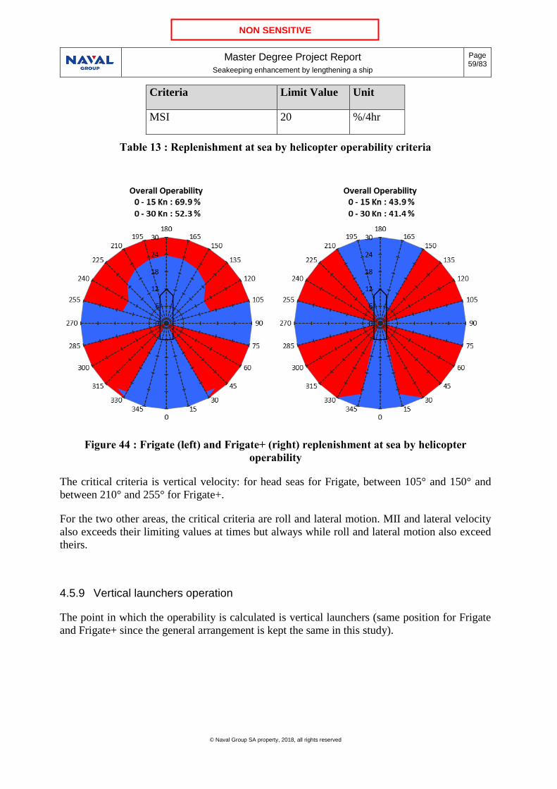
Master Degree Project Report
Seakeeping enhancement by lengthening a ship
Page 59/83
© Naval Group SA property, 2018, all rights reserved
NON SENSITIVE
Criteria Limit Value Unit
MSI 20 %/4hr
Table 13 : Replenishment at sea by helicopter operability criteria
Figure 44 : Frigate (left) and Frigate+ (right) replenishment at sea by helicopter
operability
The critical criteria is vertical velocity: for head seas for Frigate, between 105° and 150° and
between 210° and 255° for Frigate+.
For the two other areas, the critical criteria are roll and lateral motion. MII and lateral velocity
also exceeds their limiting values at times but always while roll and lateral motion also exceed
theirs.
4.5.9 Vertical launchers operation
The point in which the operability is calculated is vertical launchers (same position for Frigate
and Frigate+ since the general arrangement is kept the same in this study).

Master Degree Project Report
Seakeeping enhancement by lengthening a ship
Page 60/83
© Naval Group SA property, 2018, all rights reserved
NON SENSITIVE
Criteria Limit Value Unit
Roll 8.8 ° RMS
Pitch 1.5 ° RMS
Yaw 0.8 ° RMS
Longitudinal acceleration 0.15 g RMS
Lateral acceleration 0.35 g RMS
Vertical acceleration 0.3 g RMS
Table 14 : Vertical launchers operation operability criteria
Figure 45 : Frigate (left) and Frigate+ (right) vertical launchers operation operability
The critical criteria is yaw.
4.5.10 Torpedo tubes operation
The three rotations (roll, pitch and yaw) not being affected by the point of calculation, any point
can be used for this operability calculation (the centre of gravity is taken in this case).

Master Degree Project Report
Seakeeping enhancement by lengthening a ship
Page 61/83
© Naval Group SA property, 2018, all rights reserved
NON SENSITIVE
Criteria Limit Value Unit
Roll 3.8 ° RMS
Pitch 3.8 ° RMS
Table 15 : Torpedo tubes operation operability criteria
Figure 46 : Frigate (left) and Frigate+ (right) torpedo tubes operation operability
The critical criteria is roll.
4.5.11 Main gun operation
The point at which the operability is calculated is the main gun (same position for Frigate and
Frigate+ since the general arrangement is kept the same in this study).
Criteria Limit Value Unit
Roll 3.8 ° RMS
Pitch 3.8 ° RMS
Vertical velocity 0.5 m/s RMS
Table 16 : Main gun operation operability criteria

Master Degree Project Report
Seakeeping enhancement by lengthening a ship
Page 62/83
© Naval Group SA property, 2018, all rights reserved
NON SENSITIVE
Figure 47 : Frigate (left) and Frigate+ (right) main gun operation operability
The critical criteria for a wave heading between 45° and 75° (and between 285° and 315°) is
roll.
For all other wave headings it is vertical velocity.

Master Degree Project Report
Seakeeping enhancement by lengthening a ship
Page 63/83
© Naval Group SA property, 2018, all rights reserved
NON SENSITIVE
5 Resistance
Two different methods have been used to calculate the resistance of the two ships and thus
calculate the increase in maximum speed, with the same propulsive power, following
lengthening.
The first method consists in interpolating the ship specific resistance (total resistance divided by
the displacement) from already existing reference measures. In this instance, this interpolation
is made using the specific resistance of Figure 48 as a function of its Froude number.
The second method is the Fung method.
5.1 Using existing reference measures
Since the lengthened version has a length different from Frigate’s, its Froude number is different
at the same speed and so is its specific resistance.
Figure 48 : Frigate normalised specific resistance
So for a given speed there is a new Froude number and from this new Froude number and from
the reference curve (Figure 48), the new specific resistance is (linearly) interpolated. We can
then compare the specific resistance as a function of the speed (Figure 49).
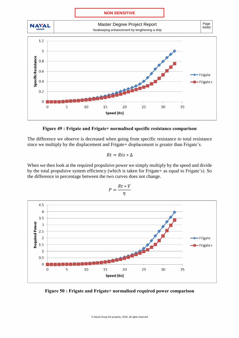
Master Degree Project Report
Seakeeping enhancement by lengthening a ship
Page 64/83
© Naval Group SA property, 2018, all rights reserved
NON SENSITIVE
Figure 49 : Frigate and Frigate+ normalised specific resistance comparison
The difference we observe is decreased when going from specific resistance to total resistance
since we multiply by the displacement and Frigate+ displacement is greater than Frigate’s.
𝑅𝑡 = 𝑅𝑡𝑠 ∗ ∆
When we then look at the required propulsive power we simply multiply by the speed and divide
by the total propulsive system efficiency (which is taken for Frigate+ as equal to Frigate’s). So
the difference in percentage between the two curves does not change.
𝑃 =𝑅𝑡 ∗ 𝑉
𝜂
Figure 50 : Frigate and Frigate+ normalised required power comparison

Master Degree Project Report
Seakeeping enhancement by lengthening a ship
Page 65/83
© Naval Group SA property, 2018, all rights reserved
NON SENSITIVE
5.2 Fung Method
The Fung method (Reference [10]) consists in determining a series of coefficients which then
are summed up to obtain a total coefficient. To each of these coefficients corresponds a
parameter. Fung has calculated the value of each coefficient depending on its corresponding
parameter value and on the additional parameter V/L (which gives a table of coefficient values).
From Fung’s measures we can then calculate by interpolation the coefficient value in our case
and obtain the resistance. The unit system used in Fung’s method is the imperial units system
and not the international units system. These different parameters (of which some are not non-
dimensional) are:
• The displacement to length ratio 𝐷𝐿 =∆
(0.01𝐿)3
• The breadth to draught ratio 𝐵𝑇 =𝐵
𝑇
• The prismatic coefficient 𝐶𝑝
• The midship section coefficient 𝐶𝑚
• The deadrise angle 𝐼𝐸
• The transom area ratio 𝑇𝐴 =𝐴20
𝐴𝑚 which is the ratio between the underwater area of station
20 (see below for station definition) and the midship section underwater area
• The transom breadth ratio 𝑇𝑊 =𝐵20
𝐵 which is the ratio between waterline breadth of
station 20 and the midship section waterline breadth
• The transom depth ratio 𝑇𝑇 =𝑇20
𝑇 which is the ratio between the draught of station 20
and the midship section draught
• The wetted surface coefficient 𝐶𝑊𝑆 =𝑊𝑆
√𝐿∆ with WS the ship wetted surface
• The bow area ratio 𝐵𝐴 =𝐴0
𝐴𝑥 which is the ratio between the underwater area of station 0
and the midship section underwater area
The « station i » used as index in some of Fung’s parameters definition corresponds to the
longitudinal position 𝐿(21−𝑖)
21. Station 0 is thus at position L and station 21 at position 0.
For the parameters TT, IE and CWS, Fung gives the following regression formulas:
𝑇𝑇 = 0.0067 + 0.3502 𝑇𝑊 − 0.4948 𝑇𝑊2 + 1.8239 𝑇𝐴 − 1.9415 𝑇𝐴2
𝐼𝐸 = 120.0192 + 69.2808
𝐷𝐿+ 0.1131
𝐿
𝐵+ 104.864
𝐵
𝐿− 28.5611 𝐶𝑝 −
26.5287
𝐶𝑝
−24.8166 𝐶𝑚 − 16.2033
𝐶𝑚+ 2.6398 𝑇𝑊 − 49.657 𝐹𝐵
𝐶𝑊𝑆 = −6.2263 − 0.0094 𝐷𝐿 + 16.0209 𝐵
𝐿+ 0.9207 𝐵𝑇 +
5.463
𝐵𝑇+ 9.8528 𝐶𝑚
+ 7.1592
𝐶𝑚
+ 0.0201 𝐼𝐸 + 2.1857
𝐼𝐸+ 1.0359 𝑇𝑊 + 2.4925 𝐵𝐴 − 3.7181 𝐹𝐵

Master Degree Project Report
Seakeeping enhancement by lengthening a ship
Page 66/83
© Naval Group SA property, 2018, all rights reserved
NON SENSITIVE
With FB being the ratio 𝐿𝐶𝐵
𝐿.
Once these parameters have been determined, we can use Fung’s data to interpolate the
coefficients. For instance, below is the Fung’s table to determine the coefficient associated to the
parameter BT.
Table 17 : Fung’s residuary resistance coefficient component table
After the different coefficients are determined, they are summed to get a total coefficient 𝐶𝑅.
From this coefficient we can calculate the residuary resistance RR to which we will have to add
the viscous resistance in order to obtain the ship total resistance.
𝑅𝑅 =1
2𝜌 𝑊𝑆 𝑉2 𝐶𝑅

Master Degree Project Report
Seakeeping enhancement by lengthening a ship
Page 67/83
© Naval Group SA property, 2018, all rights reserved
NON SENSITIVE
Figure 51 : Frigate and Frigate+ normalised residuary resistance comparison
5.3 Speed and Power
The viscous resistance is not given by Fung’s method and is calculated with a regression
formula:
𝑅𝑓 = 𝑓(𝑊𝑆, 𝐿, ∆, 𝑉)
We then get the required engine power with the propulsive system efficiency:
𝑃 = (𝑅𝑅 + 𝑅𝑓) 𝑉
𝜂
We can now plot the curves of the two ships propulsive power, calculated with the two methods,
as a function of their speed. This allows us to determine the maximum speed that the ship can
reach for a given installed power.

Master Degree Project Report
Seakeeping enhancement by lengthening a ship
Page 68/83
© Naval Group SA property, 2018, all rights reserved
NON SENSITIVE
Figure 52 : Frigate and Frigate+ normalised required power comparison
If we choose as installed power the power of Frigate’s actual propulsion system, we get the
following maximum speed results:
Maximum Speed (kn) Measures Fung
Frigate 24.0 25.1
Frigate+ 25.2 26.7
Table 18 : Maximum speed comparison for same engine power
So we can increase the speed by 1 kn in both cases (and even 1.5 kn with Fung’s method).
It is also possible to choose to keep the same maximum speed requirement (25 kn) and to
reduce the power to be installed.

Master Degree Project Report
Seakeeping enhancement by lengthening a ship
Page 69/83
© Naval Group SA property, 2018, all rights reserved
NON SENSITIVE
Required Power Measures Fung
Cruise speed : 15 kn
Frigate 0.202 0.172
Frigate+ 0.176 0.175
Variation (%) -12.9 +1.74
Current maximum speed : 25 kn
Frigate 1.205 0.985
Frigate+ 0.975 0.814
Variation (%) -19.1 -17.4
Maximum speed : 27 kn
Frigate 1.796 1.405
Frigate+ 1.287 1.042
Variation (%) -28.3 -25.8
Maximum speed : 30 kn
Frigate 2.858 2.198
Frigate+ 2.163 1.578
Variation (%) -24.3 -28.2
Table 19 : Normalised engine power comparison for same speed
For the cruise speed of 15 kn, the measures data gives a reduction of the required power of 13%
while the Fung method gives a required power approximately equal. For higher speeds, possible
maximum speeds for the lengthened frigate, the reduction given by the two methods is similar.
For 25 kn, the current maximum speed, the reduction is almost 20% and for even higher speeds
it is even more important, it is over 25% and approaches 30%.

Master Degree Project Report
Seakeeping enhancement by lengthening a ship
Page 70/83
© Naval Group SA property, 2018, all rights reserved
NON SENSITIVE
6 Costs
A Naval Group cost engineer has made a first cost estimate of the lengthened hull as 25% more
expensive than the reference one. Usually, hull costs represent about 15% of the total frigate
purchase cost which gives us an increase of total cost of 3.8%. This estimation is close to the
calculations made for a patroller (Reference [7]) which give an increase of 3% of building costs.
Besides this increase in building cost, there is a reduction in operational costs. Indeed, the
reduction in required power for a same speed leads to a decrease in fuel consumption (and may
also lead to the purchase of a smaller and cheaper engine). Knowing the price of fuel, the engine
fuel consumption and the operational profile of the reference frigate it is possible to calculate the
cost reduction. However, at the time of this report, the reference frigate operational profile had
not yet been acquired. Thus, this decrease in operational cost, which may or may not compensate
the increase in building cost overall the frigate lifespan, has not been estimated.

Master Degree Project Report
Seakeeping enhancement by lengthening a ship
Page 71/83
© Naval Group SA property, 2018, all rights reserved
NON SENSITIVE
7 Conclusion
The concept of lengthened version of a reference ship developed in this study requires a few
transformations on the hull form and not just a basic homothety. After having modified the hull
form, and having estimated the lengthened ship mass, seakeeping and operability were
calculated. The seakeeping results showed a significant decrease in pitch, from 35% to 15%
depending on the sea state. However, the operability results do not really show an improvement
which seems to indicate that despite the fact that the sailors regard pitch as the worst motion
which thus has to be reduced, it is not the critical criteria for operability. Moreover, the lack of
roll damping fins implementation in the seakeeping model leads to roll being higher than it is
supposed to be and thus to the appearance of red areas in operability graphs where roll exceeds
its limit value whereas it should not.
With regard to the costs of such a lengthened ship, the building costs increase by a few percent.
The lengthened ship’s resistance is lower than the reference ship’s which means a decrease in
fuel consumption and thus a reduction of operational costs. This reduction still needs to be
estimated and compared to the increase in building costs to see whether or not they balance each
other during the lifespan of the ship. This potential through life cost reduction would come as a
“bonus” to the increased seakeeping performance of the lengthened ship.

Master Degree Project Report
Seakeeping enhancement by lengthening a ship
Page 72/83
© Naval Group SA property, 2018, all rights reserved
NON SENSITIVE
8 References
[1] Frigate Captain Laurent Célérier, Marine de guerre : le retour des navires à grande
vitesse ?, Marine & Océans, February 24th 2012.
[2] Benoît Quesson, Développement d’un outil de prédimensionnement de bâtiments de
surface, Degree Project, Ecole Nationale Supérieure des Techniques Avancées de
Bretagne, 2014.
[3] H. Lackenby, On the Systematic Geometrical Variation of Ship Forms, 1950.
[4] STANAG 4194 Standardized Waves and Wind Environments, Edition 1 including Amdt
5, April 1984
[5] STANAG 4154 Common Procedures for Seakeeping in the Ship Design Process, Edition
3, December 13th 2003.
[6] Alexander Keuning, Serge Toxopeus, Jakob Pinkster, The Effect of Bowshape on the
Seakeeping Performance of a Fast Monohull, 2001.
[7] J.A Keuning, Jakob Pinkster, Further Design and Seakeeping Investigations into
“Enlarged Ship Concept”, Fourth International Conference on Fast Sea Transportation
FAST’97, Sydney, Australia, 21, 22 and 23 July 1997.
[8] J.A Keuning, From Idea to Reality: The “Enlarged Ship Concept”, Schip en Werf De Zee,
May 2000.
[9] Thomas Eefsen & Al, Development of Frigate Designs with good Seakeeping
Characteristics, 9th Symposium on Practical Design of Ships and Other Floating
Structures, Luebeck-Travemuende, Germany, 2004.
[10] Justin C. Hlavin, Hydrostatic and Hydrodynamic analysis of a lengthened DDG-51
Destroyer Modified Repeat, Thesis, Naval Postgraduate School, 2010.
[11] Siu C. Fung, Resistance and Powering Prediction for Transom Stern Hull Forms During
Early Stage Ship Design, SNAME Transactions Vol. 99, 1991, pp. 29-84.
[12] Michel K. Ochi, Lewis E. Motter, Prediction of Slamming Characteristics and Hull
Responses for Ship Design, SNAME Transactions Vol. 81, 1973, pp. 144-176.
[13] James F. O’Hanlon, Michael E. McCauley, Motion Sickness Incidence as a Function of
the Frequency and Acceleration of Vertical Sinusoidal Motion, Humans Factor Research,
1974.
Master Degree Project Report
Seakeeping enhancement by lengthening a ship
Page 73/83
© Naval Group SA property, 2018, all rights reserved
NON SENSITIVE
[14] J.M.Riola, S.Esteban, J.M.Girón-Sierra, J.Aranda, Motion and Seasickness of Fast
Warships, NATO, 2004.
[15] Tomasz Cepowski, The Prediction of the Motion Sickness Incidence Index at the Initial
Design Stage, Scientific Journal of the University of Szczecin, 2012, 31(103) pp. 45-48.
[16] Lauren W.Hanyok, Methods for Calculating Motion Induced Interruptions as Applied to
a Space Capsule After Splashdown, Master Thesis, Virginia Polytechnic Institute and State
University, 2012.
[17] Theory Manual Precal_R version 16.2.0, Marin, June 13th 2017.

Master Degree Project Report
Seakeeping enhancement by lengthening a ship
Page 74/83
© Naval Group SA property, 2018, all rights reserved
NON SENSITIVE
9 Appendices
9.1 Appendix 1: Proof of the variation of LCB via a « swinging » of the sectional area curve
For a required δLCB, the transformation given is: 𝑥𝑛𝑒𝑤 = 𝑥 + 𝛿𝑥 = 𝑥 + 𝑦 tan𝜃 where y is the
y coordinate of the sectional area curve and tan 𝜃 =𝛿𝐿𝐶𝐵
�̅� where �̅� is the y coordinate of the
centroid of the sectional area curve. This transformation has the property to give δx = 0 for x =
0 and x = L (so Lnew = L) since y = 0 for these positions.
A necessary preliminary calculation, which is detailed below, is the proof of the displacement
conservation. Knowing that 𝑦𝑛𝑒𝑤(𝑥𝑛𝑒𝑤) = 𝑦(𝑥) (which will simply be noted y below), we can
write:
𝛻𝑛𝑒𝑤 = ∫ 𝑦𝑛𝑒𝑤(𝑥𝑛𝑒𝑤)𝑑𝑥𝑛𝑒𝑤
𝐿𝑛𝑒𝑤
0
= ∫ 𝑦(1 + 𝑦′𝐿
0
tan 𝜃)𝑑𝑥
= ∫ 𝑦𝑑𝑥𝐿
0
+∫ 𝑦𝑦′ tan 𝜃 𝑑𝑥𝐿
0
= 𝛻 + tan𝜃 [𝑦2
2]0
𝐿
= 𝛻
𝐿𝐶𝐵𝑛𝑒𝑤 =∫ 𝑦𝑛𝑒𝑤(𝑥𝑛𝑒𝑤)𝑥𝑛𝑒𝑤𝑑𝑥𝑛𝑒𝑤𝐿𝑛𝑒𝑤0
∫ 𝑦𝑛𝑒𝑤(𝑥𝑛𝑒𝑤)𝑑𝑥𝑛𝑒𝑤𝐿𝑛𝑒𝑤
0
= 1
𝛻𝑛𝑒𝑤∫ 𝑦𝑛𝑒𝑤(𝑥𝑛𝑒𝑤)𝑥𝑛𝑒𝑤𝑑𝑥𝑛𝑒𝑤
𝐿𝑛𝑒𝑤
0
=1
𝛻∫ 𝑦(𝑥 + 𝑦𝐿
0
tan 𝜃)(1 + 𝑦′ tan 𝜃)𝑑𝑥
=1
𝛻∫ (𝑦𝑥 + 𝑦𝑥𝑦′ tan 𝜃 + 𝑦2 tan 𝜃 + 𝑦2𝑦′ tan2 𝜃)𝐿
0
𝑑𝑥
= 1
𝛻∫ 𝑦𝑥𝑑𝑥𝐿
0
+tan𝜃
𝛻∫ (𝑦𝑥𝑦′ + 𝑦2 + 𝑦2𝑦′ tan 𝜃)𝑑𝑥𝐿
0
= 𝐿𝐶𝐵 +tan 𝜃
𝛻∫ (𝑦𝑥𝑦′ + 𝑦2 + 𝑦2𝑦′ tan 𝜃)𝑑𝑥𝐿
0
Since 𝑦(𝑥 = 0) = 𝑦(𝑥 = 𝐿) = 0. we have:
∫ 𝑦𝑥𝑦′𝑑𝑥 = [𝑥𝑦2
2]0
𝐿
−∫𝑦2
2𝑑𝑥
𝐿
0
𝐿
0
= −∫𝑦2
2𝑑𝑥
𝐿
0

Master Degree Project Report
Seakeeping enhancement by lengthening a ship
Page 75/83
© Naval Group SA property, 2018, all rights reserved
NON SENSITIVE
𝐿𝐶𝐵𝑛𝑒𝑤 = 𝐿𝐶𝐵 +tan 𝜃
𝛻∫ (
𝑦2
2+ 𝑦2𝑦′ tan 𝜃)𝑑𝑥
𝐿
0
= 𝐿𝐶𝐵 +tan 𝜃
𝛻∫𝑦2
2𝑑𝑥
𝐿
0
+tan2 𝜃
𝛻[𝑦3
3]0
𝐿
= 𝐿𝐶𝐵 +tan 𝜃
𝛻∫𝑦2
2𝑑𝑥
𝐿
0
And
�̅� = ∫ ∫ 𝑦𝑑𝑦𝑑𝑥
𝑦(𝑥)
0
𝐿
0
∫ ∫ 𝑑𝑦𝑑𝑥𝑦(𝑥)
0
𝐿
0
= ∫𝑦2
2 𝑑𝑥𝐿
0
∫ 𝑦𝑑𝑥𝐿
0
=∫𝑦2
2 𝑑𝑥𝐿
0
𝛻
So:
𝐿𝐶𝐵𝑛𝑒𝑤 = 𝐿𝐶𝐵 +tan 𝜃
𝛻�̅�𝛻
= 𝐿𝐶𝐵 + 𝛿𝐿𝐶𝐵
After transformation, the variation in LCB is really the required δLCB.

Master Degree Project Report
Seakeeping enhancement by lengthening a ship
Page 76/83
© Naval Group SA property, 2018, all rights reserved
NON SENSITIVE
9.2 Appendix 2: Formulas for the deformation of a section
The idea behind this deformation is to ensure that the new underwater cross-section is a
transformation of the old underwater cross-section only and, similarly, that the new above water
cross-section is a transformation of the old above water cross-section only.
This transformation of a section consists in a multiplication of the two parts (underwater and
above water) of the old section by a polynomial of degree 2 in z for the underwater cross-section
and degree 1 for the above water cross-section and in an adjustment of the z coordinates related
to the new values Tnew et Cnew. This can be written:
• For z ≤ T : 𝐵𝑛𝑒𝑤(𝑧𝑛𝑒𝑤) = 𝐵(𝑧)(𝑐1𝑧𝑛𝑒𝑤2 + 𝑐2𝑧𝑛𝑒𝑤 + 𝑐3)
znew must verify: {𝑧𝑛𝑒𝑤(𝑧 = 0) = 0
𝑧𝑛𝑒𝑤(𝑧 = 𝑇) = 𝑇𝑛𝑒𝑤
By choosing znew as a linear function of z. we get: 𝑧𝑛𝑒𝑤 =𝑧𝑇𝑛𝑒𝑤
𝑇
• For z ≥ T : 𝐵𝑛𝑒𝑤(𝑧𝑛𝑒𝑤) = 𝐵(𝑧)(𝑎𝑧𝑛𝑒𝑤 + 𝑏)
znew must verify: {𝑧𝑛𝑒𝑤(𝑧 = 𝑇) = 𝑇𝑛𝑒𝑤 𝑧𝑛𝑒𝑤(𝑧 = 𝐶) = 𝐶𝑛𝑒𝑤
By choosing znew as a linear function of z. we get: 𝑧𝑛𝑒𝑤 =(𝑧−𝑇)(𝐶𝑛𝑒𝑤−𝑇𝑛𝑒𝑤)
𝐶−𝑇+ 𝑇𝑛𝑒𝑤
The improvement I personally added to this method is as follow. Previously only the a and b
coefficients were determined as well as c2 as a function of c1 and c3. c1 and c3 were then given
an initial default value which was then modified by arbitrary increment until reaching.
theoretically. a satisfying section. This method restricted the range of possible values taken by
c1 and c3 (and so c2 too) and the variation of these coefficients at each increment was done
arbitrarily. For instance. if the underwater area of the section was too high c1 was modified until
it reached a fixed limit after which c3 was modified and then c1 again. After the improvement.
all five coefficients are directly determined. There no longer is an incremental search for a section
which may not be found. The satisfying section is now directly determined which results in a
substantial calculations time reduction.
Determination of a and b
The two conditions used to determine a and b are {𝐵𝑛𝑒𝑤(𝑇𝑛𝑒𝑤) = 𝐵𝑛𝑒𝑤
𝐵𝑛𝑒𝑤(𝐶𝑛𝑒𝑤) = 𝐵𝑜𝑎 𝑛𝑒𝑤
This corresponds to making it so that the above water part of the section respects the new
dimensions required so making the breadth equal to the waterline breadth required for a height
equal to the required draught and the breadth equal to the overall breadth required for a height
equal to the required depth.
For this method. the overall breadth Boa refers to the breadth at a height equal to the depth of the
ship even though for fighting ships the overall breadth is at a height lower than the depth.

Master Degree Project Report
Seakeeping enhancement by lengthening a ship
Page 77/83
© Naval Group SA property, 2018, all rights reserved
NON SENSITIVE
𝑎(𝐶𝑛𝑒𝑤 − 𝑇𝑛𝑒𝑤) =𝐵𝑜𝑎 𝑛𝑒𝑤𝐵𝑜𝑎
−𝐵𝑛𝑒𝑤𝐵
𝑏 =𝐵𝑛𝑒𝑤𝐵
− 𝑎𝑇𝑛𝑒𝑤
𝐶𝑛𝑒𝑤 − 𝑇𝑛𝑒𝑤
=1
𝐶𝑛𝑒𝑤 − 𝑇𝑛𝑒𝑤(𝐵𝑛𝑒𝑤𝐵
(𝐶𝑛𝑒𝑤 − 𝑇𝑛𝑒𝑤) − 𝑇𝑛𝑒𝑤𝐵𝑜𝑎 𝑛𝑒𝑤𝐵𝑜𝑎
+ 𝑇𝑛𝑒𝑤𝐵𝑛𝑒𝑤𝐵)
= 1
𝐶𝑛𝑒𝑤 − 𝑇𝑛𝑒𝑤(𝐵𝑛𝑒𝑤𝐵
𝐶𝑛𝑒𝑤 −𝐵𝑜𝑎 𝑛𝑒𝑤𝐵𝑜𝑎
𝑇𝑛𝑒𝑤)
For z ≥ T we then have:
𝐵𝑛𝑒𝑤(𝑧𝑛𝑒𝑤) =𝐵(𝑧)
𝐶𝑛𝑒𝑤 − 𝑇𝑛𝑒𝑤(𝑧𝑛𝑒𝑤 (
𝐵𝑜𝑎 𝑛𝑒𝑤𝐵𝑜𝑎
−𝐵𝑛𝑒𝑤𝐵) +
𝐵𝑛𝑒𝑤𝐵
𝐶𝑛𝑒𝑤 −𝐵𝑜𝑎 𝑛𝑒𝑤𝐵𝑜𝑎
𝑇𝑛𝑒𝑤)
With 𝑧𝑛𝑒𝑤 =(𝑧−𝑇)(𝐶𝑛𝑒𝑤−𝑇𝑛𝑒𝑤)
𝐶−𝑇+ 𝑇𝑛𝑒𝑤
Determination of c1. c2 and c3
The three conditions used to determine c1. c2 and c3 are:
1. Underwater area of the new section equal to the required area (improvement)
2. Continuity in znew = Tnew of the new section that is to say no discontinuity in the hull
(condition already used in a previous work)
3. Continuity in znew = Tnew of the slope of the new section that is to say no hard chine in the
hull (improvement)
It is not possible to use the condition: same value of z at a breadth equal to 0 for the new and the
old section. This condition corresponds to both sections having the same point on the axis y =
0. However. for most sections. the first coordinate in B(z) is 0. The equation would then become
0 = 0 × (𝑐1𝑧𝑛𝑒𝑤2 + 𝑐2𝑧𝑛𝑒𝑤 + 𝑐3) and would not give any condition on the coefficients.
• Underwater area condition
𝐴𝑥 = ∫ 𝐵𝑛𝑒𝑤(𝑧𝑛𝑒𝑤)𝑑𝑧𝑛𝑒𝑤
𝑇𝑛𝑒𝑤
0
= ∫ 𝐵(𝑧)(𝑐1𝑧𝑛𝑒𝑤2 + 𝑐2𝑧𝑛𝑒𝑤 + 𝑐3)𝑑𝑧𝑛𝑒𝑤
𝑇𝑛𝑒𝑤
0
= ∫ 𝐵(𝑧) (𝑐1 (𝑧𝑇𝑛𝑒𝑤𝑇
)2
+ 𝑐2 (𝑧𝑇𝑛𝑒𝑤𝑇
) + 𝑐3)𝑇𝑛𝑒𝑤𝑇𝑑𝑧
𝑇
0
𝑐1 (𝑇𝑛𝑒𝑤𝑇)3
∫ 𝐵(𝑧)𝑧2𝑑𝑧 + 𝑐2 (𝑇𝑛𝑒𝑤𝑇)2
∫ 𝐵(𝑧)𝑧𝑑𝑧 + 𝑐3𝑇𝑛𝑒𝑤𝑇∫ 𝐵(𝑧)𝑑𝑧𝑇
0
𝑇
0
𝑇
0
= 𝐴

Master Degree Project Report
Seakeeping enhancement by lengthening a ship
Page 78/83
© Naval Group SA property, 2018, all rights reserved
NON SENSITIVE
• Continuity condition
𝐵𝑛𝑒𝑤(𝑇𝑛𝑒𝑤) = 𝐵(𝑇)(𝑐1𝑇𝑛𝑒𝑤2 + 𝑐2𝑇𝑛𝑒𝑤 + 𝑐3)
𝑐1𝑇𝑛𝑒𝑤2 + 𝑐2𝑇𝑛𝑒𝑤 + 𝑐3 =
𝐵𝑛𝑒𝑤𝐵
• Slope continuity condition
𝑑𝐵𝑛𝑒𝑤𝑑𝑧
(𝑧 ≤ 𝑇)
= 𝐵(𝑧)(2𝑐1𝑧 (𝑇𝑛𝑒𝑤𝑇)2
+ 𝑐2 (𝑇𝑛𝑒𝑤𝑇))
+ 𝐵′(𝑧) (𝑐1 (𝑧𝑇𝑛𝑒𝑤𝑇
)2
+ 𝑐2 (𝑧𝑇𝑛𝑒𝑤𝑇
) + 𝑐3)
𝑑𝐵𝑛𝑒𝑤𝑑𝑧
(𝑧 ≥ 𝑇)
= 𝐵(𝑧) (1
𝐶𝑛𝑒𝑤 − 𝑇𝑛𝑒𝑤(𝐵𝑜𝑎 𝑛𝑒𝑤𝐵𝑜𝑎
−𝐵𝑛𝑒𝑤𝐵)𝐶𝑛𝑒𝑤 − 𝑇𝑛𝑒𝑤𝐶 − 𝑇
)
+𝐵′(𝑧)
𝐶𝑛𝑒𝑤 − 𝑇𝑛𝑒𝑤((𝐵𝑜𝑎 𝑛𝑒𝑤𝐵𝑜𝑎
−𝐵𝑛𝑒𝑤𝐵)((𝑧 − 𝑇)(𝐶𝑛𝑒𝑤 − 𝑇𝑛𝑒𝑤)
𝐶 − 𝑇+ 𝑇𝑛𝑒𝑤)
+𝐵𝑛𝑒𝑤𝐵
𝐶𝑛𝑒𝑤 −𝐵𝑜𝑎 𝑛𝑒𝑤𝐵𝑜𝑎
𝑇𝑛𝑒𝑤)
These two expressions must be equal for z = T which gives us:
𝐵 (2𝑐1𝑇𝑛𝑒𝑤2
𝑇+ 𝑐2
𝑇𝑛𝑒𝑤𝑇) + 𝐵′(𝑇)(𝑐1𝑇𝑛𝑒𝑤
2 + 𝑐2𝑇𝑛𝑒𝑤 + 𝑐3)
=𝐵
𝐶 − 𝑇(𝐵𝑜𝑎 𝑛𝑒𝑤𝐵𝑜𝑎
−𝐵𝑛𝑒𝑤𝐵)
+𝐵′(𝑇)
𝐶𝑛𝑒𝑤 − 𝑇𝑛𝑒𝑤(𝑇𝑛𝑒𝑤 (
𝐵𝑜𝑎 𝑛𝑒𝑤𝐵𝑜𝑎
−𝐵𝑛𝑒𝑤𝐵) +
𝐵𝑛𝑒𝑤𝐵
𝐶𝑛𝑒𝑤 −𝐵𝑜𝑎 𝑛𝑒𝑤𝐵𝑜𝑎
𝑇𝑛𝑒𝑤)
𝑐1 (2𝐵𝑇𝑛𝑒𝑤2
𝑇+ 𝐵′(𝑇)𝑇𝑛𝑒𝑤
2 ) + 𝑐2 (𝐵𝑇𝑛𝑒𝑤𝑇+ 𝐵′(𝑇)𝑇𝑛𝑒𝑤) + 𝑐3𝐵
′(𝑇)
=𝐵
𝐶 − 𝑇(𝐵𝑜𝑎 𝑛𝑒𝑤𝐵𝑜𝑎
−𝐵𝑛𝑒𝑤𝐵) +
𝐵′(𝑇)𝐵𝑛𝑒𝑤𝐵
These three conditions can be written in matrix format AC = B:
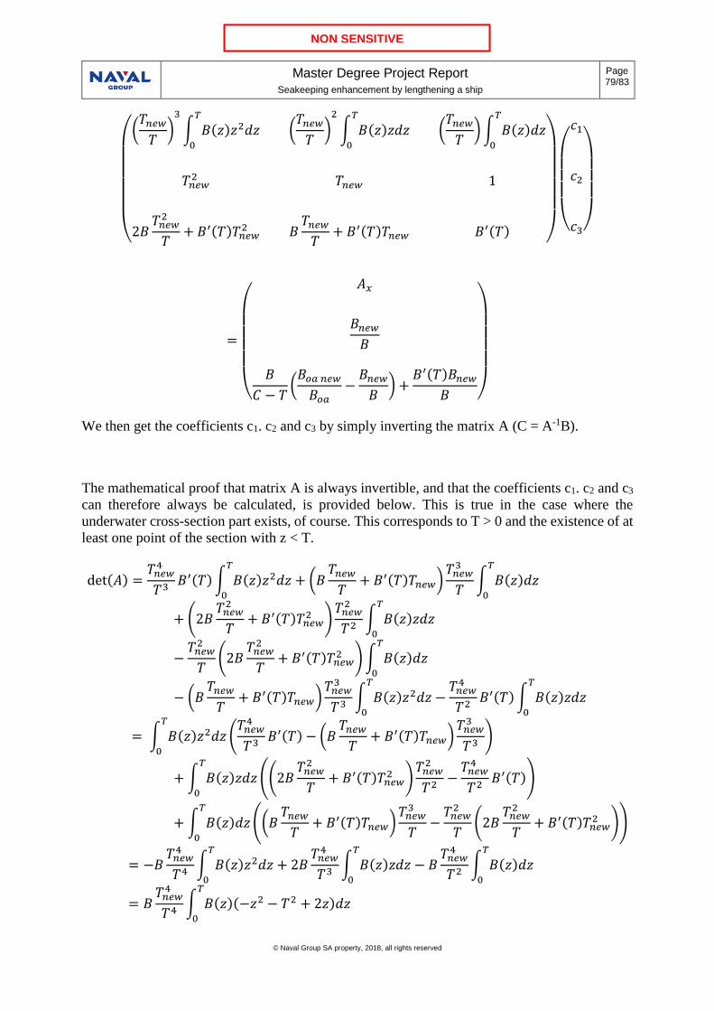
Master Degree Project Report
Seakeeping enhancement by lengthening a ship
Page 79/83
© Naval Group SA property, 2018, all rights reserved
NON SENSITIVE
(
(𝑇𝑛𝑒𝑤𝑇)3
∫ 𝐵(𝑧)𝑧2𝑑𝑧𝑇
0
(𝑇𝑛𝑒𝑤𝑇)2
∫ 𝐵(𝑧)𝑧𝑑𝑧𝑇
0
(𝑇𝑛𝑒𝑤𝑇)∫ 𝐵(𝑧)𝑑𝑧
𝑇
0
𝑇𝑛𝑒𝑤2 𝑇𝑛𝑒𝑤 1
2𝐵𝑇𝑛𝑒𝑤2
𝑇+ 𝐵′(𝑇)𝑇𝑛𝑒𝑤
2 𝐵𝑇𝑛𝑒𝑤𝑇+ 𝐵′(𝑇)𝑇𝑛𝑒𝑤 𝐵′(𝑇) )
(
𝑐1
𝑐2
𝑐3)
=
(
𝐴𝑥
𝐵𝑛𝑒𝑤𝐵
𝐵
𝐶 − 𝑇(𝐵𝑜𝑎 𝑛𝑒𝑤𝐵𝑜𝑎
−𝐵𝑛𝑒𝑤𝐵) +
𝐵′(𝑇)𝐵𝑛𝑒𝑤𝐵 )
We then get the coefficients c1. c2 and c3 by simply inverting the matrix A (C = A-1B).
The mathematical proof that matrix A is always invertible, and that the coefficients c1. c2 and c3
can therefore always be calculated, is provided below. This is true in the case where the
underwater cross-section part exists, of course. This corresponds to T > 0 and the existence of at
least one point of the section with z < T.
det(𝐴) =𝑇𝑛𝑒𝑤4
𝑇3𝐵′(𝑇)∫ 𝐵(𝑧)𝑧2𝑑𝑧
𝑇
0
+ (𝐵𝑇𝑛𝑒𝑤𝑇+ 𝐵′(𝑇)𝑇𝑛𝑒𝑤)
𝑇𝑛𝑒𝑤3
𝑇∫ 𝐵(𝑧)𝑑𝑧𝑇
0
+ (2𝐵𝑇𝑛𝑒𝑤2
𝑇+ 𝐵′(𝑇)𝑇𝑛𝑒𝑤
2 )𝑇𝑛𝑒𝑤2
𝑇2∫ 𝐵(𝑧)𝑧𝑑𝑧𝑇
0
−𝑇𝑛𝑒𝑤2
𝑇(2𝐵
𝑇𝑛𝑒𝑤2
𝑇+ 𝐵′(𝑇)𝑇𝑛𝑒𝑤
2 )∫ 𝐵(𝑧)𝑑𝑧𝑇
0
− (𝐵𝑇𝑛𝑒𝑤𝑇+ 𝐵′(𝑇)𝑇𝑛𝑒𝑤)
𝑇𝑛𝑒𝑤3
𝑇3∫ 𝐵(𝑧)𝑧2𝑑𝑧𝑇
0
−𝑇𝑛𝑒𝑤4
𝑇2𝐵′(𝑇)∫ 𝐵(𝑧)𝑧𝑑𝑧
𝑇
0
= ∫ 𝐵(𝑧)𝑧2𝑑𝑧𝑇
0
(𝑇𝑛𝑒𝑤4
𝑇3𝐵′(𝑇) − (𝐵
𝑇𝑛𝑒𝑤𝑇+ 𝐵′(𝑇)𝑇𝑛𝑒𝑤)
𝑇𝑛𝑒𝑤3
𝑇3)
+ ∫ 𝐵(𝑧)𝑧𝑑𝑧𝑇
0
((2𝐵𝑇𝑛𝑒𝑤2
𝑇+ 𝐵′(𝑇)𝑇𝑛𝑒𝑤
2 )𝑇𝑛𝑒𝑤2
𝑇2−𝑇𝑛𝑒𝑤4
𝑇2𝐵′(𝑇))
+ ∫ 𝐵(𝑧)𝑑𝑧𝑇
0
((𝐵𝑇𝑛𝑒𝑤𝑇+ 𝐵′(𝑇)𝑇𝑛𝑒𝑤)
𝑇𝑛𝑒𝑤3
𝑇−𝑇𝑛𝑒𝑤2
𝑇(2𝐵
𝑇𝑛𝑒𝑤2
𝑇+ 𝐵′(𝑇)𝑇𝑛𝑒𝑤
2 ))
= −𝐵𝑇𝑛𝑒𝑤4
𝑇4∫ 𝐵(𝑧)𝑧2𝑑𝑧𝑇
0
+ 2𝐵𝑇𝑛𝑒𝑤4
𝑇3∫ 𝐵(𝑧)𝑧𝑑𝑧𝑇
0
− 𝐵𝑇𝑛𝑒𝑤4
𝑇2∫ 𝐵(𝑧)𝑑𝑧𝑇
0
= 𝐵𝑇𝑛𝑒𝑤4
𝑇4∫ 𝐵(𝑧)(−𝑧2 − 𝑇2 + 2𝑧)𝑑𝑧𝑇
0

Master Degree Project Report
Seakeeping enhancement by lengthening a ship
Page 80/83
© Naval Group SA property, 2018, all rights reserved
NON SENSITIVE
= −𝐵 (𝑇𝑛𝑒𝑤
𝑇)4
∫ 𝐵(𝑧)(𝑧 − 𝑇)2𝑑𝑧𝑇
0< 0
The determinant of the matrix is not null; the matrix is thus always invertible.

Master Degree Project Report
Seakeeping enhancement by lengthening a ship
Page 81/83
© Naval Group SA property, 2018, all rights reserved
NON SENSITIVE
9.3 Appendix 3: Hull girder strengthening effective length
The effective length 𝐿𝑒𝑓𝑓, as illustrated below, is defined as the length for which the area between
the two bending moment curves 𝑀𝑓𝑛𝑒𝑤(𝑥) and 𝑀𝑓(𝑥) is equal to the area between the curve
𝑀𝑓(𝑥) and the curve equal to 𝑀𝑓(𝑥) to which is added 𝑀𝑓𝑛𝑒𝑤 𝑚𝑎𝑥 −𝑀𝑓𝑚𝑎𝑥 over that length i.e.
equality of the two orange areas shown in Figure 53.
⇕
Figure 53 : Illustration of the effective length definition
∫ (𝑀𝑓𝑛𝑒𝑤(𝑥) − 𝑀𝑓(𝑥))𝑑𝑥𝐿
0
= 𝐿𝑒𝑓𝑓(𝑀𝑓𝑛𝑒𝑤 𝑚𝑎𝑥 −𝑀𝑓𝑚𝑎𝑥)
We then make the assumption that 𝑀𝑓𝑛𝑒𝑤(𝑥) =𝑀𝑓𝑛𝑒𝑤 𝑚𝑎𝑥
𝑀𝑓𝑚𝑎𝑥𝑀𝑓(𝑥) so we have:

Master Degree Project Report
Seakeeping enhancement by lengthening a ship
Page 82/83
© Naval Group SA property, 2018, all rights reserved
NON SENSITIVE
𝐿𝑒𝑓𝑓(𝑀𝑓𝑛𝑒𝑤 𝑚𝑎𝑤 −𝑀𝑓𝑚𝑎𝑥) = ∫ (𝑀𝑓𝑛𝑒𝑤 𝑚𝑎𝑥𝑀𝑓𝑚𝑎𝑥
− 1)𝑀𝑓(𝑥)𝑑𝑥𝐿
0
𝐿𝑒𝑓𝑓 = ∫𝑀𝑓(𝑥)
𝑀𝑓𝑚𝑎𝑥𝑑𝑥
𝐿
0
The effective length does not depend on the variation applied to the bending moment curve
anymore. To one curve we can associate one effective length independent of the applied
variation.
We then study the relation between effective lengths of two curves 1 and 2 so that 𝑀𝑓1 ≤ 𝑀𝑓2
and 𝑀𝑓1 𝑚𝑎𝑥 = 𝑀𝑓2 𝑚𝑎𝑥
Figure 54: Comparison of two bending moments
𝐿𝑒𝑓𝑓1 = ∫𝑀𝑓1(𝑥)
𝑀𝑓1 𝑚𝑎𝑥𝑑𝑥
𝐿
0
≤ ∫𝑀𝑓2(𝑥)
𝑀𝑓1 𝑚𝑎𝑥𝑑𝑥
𝐿
0
= 𝐿𝑒𝑓𝑓2
So, if the Frigate bending moment curve fits between two bending moment curves (having the
same maximum bending moment as Frigate) then we will have a lower and upper boundary for
the effective length associated to the Frigate bending moment curve.
The bending moment is null at 0 and L and its maximum is 𝑀𝑓𝑚𝑎𝑥 at 𝐿
2. The simplest function
verifying these conditions is 𝑓(𝑥) = 𝑀𝑓𝑚𝑎𝑥𝑥(𝐿 − 𝑥)4
𝐿2
We use the indexed family of functions 𝑓𝑛(𝑥) = 𝑀𝑓𝑚𝑎𝑥𝑥𝑛(𝐿 − 𝑥)𝑛 (
2
𝐿)2𝑛
to “surround” the
Frigate bending moment curve.

Master Degree Project Report
Seakeeping enhancement by lengthening a ship
Page 83/83
© Naval Group SA property, 2018, all rights reserved
NON SENSITIVE
The Frigate bending moment curve used is the following one (in light green). It corresponds to
the load case which induces the highest bending moment. Bending moment curves induced by
other load cases are thus not shown on the following graphs.
Figure 55: Frigate highest bending moment curve
Figure 56: Frigate highest bending moment curve and the family of functions curves
We can then calculate:
𝐿𝑒𝑓𝑓𝑛 = (2
𝐿)2𝑛
∫ 𝑥𝑛(𝐿 − 𝑥)𝑛𝑑𝑥𝐿
0
n 1 2 3 4
𝛼 =𝐿𝑒𝑓𝑓
𝐿⁄ 0.666 0.533 0.457 0.406
Table 20 : Effective length to length ratio
Since the Frigate curve is between curves 2 and 3 and much closer to 3, we choose 𝛼𝐹𝐿𝐹 = 0.47

TRITA TRITA-SCI-GRU 2018:020
www.kth.se