arX

iv:1

108.

4372

v1 [

astr

o-ph

.CO

] 22

Aug

201

1Astronomy & Astrophysicsmanuscript no. AA17529 c© ESO 2011August 23, 2011

SDSS DR7 superclustersPrincipal component analysis

M. Einasto1, L.J. Liivamagi1,2, E. Saar1,3, J. Einasto1,3,4, E. Tempel1, E. Tago1, and V.J. Martınez5

1 Tartu Observatory, 61602 Toravere, Estonia2 Institute of Physics, Tartu University, Tahe 4, 51010 Tartu, Estonia3 Estonian Academy of Sciences, EE-10130 Tallinn, Estonia4 ICRANet, Piazza della Repubblica 10, 65122 Pescara, Italy5 Observatori Astronomic, Universitat de Valencia, Apartat de Correus 22085, E-46071 Valencia, Spain

Received .../ Accepted ...

ABSTRACT

Context. The study of superclusters of galaxies helps us to understand the formation, evolution, and present-day properties of thelarge-scale structure of the Universe.Aims. We use data about superclusters drawn from the SDSS DR7 to analyse possible selection effects in the supercluster catalogue,to study the physical and morphological properties of superclusters, to find their possible subsets, and to determine scaling relationsfor our superclusters.Methods. We apply principal component analysis and Spearman’s correlation test to study the properties of superclusters.Results. We have found that the parameters of superclusters do not correlate with their distance. The correlations between the physicaland morphological properties of superclusters are strong.Superclusters can be divided into two populations according to their totalluminosity: high-luminosity ones withLg > 400 1010h−2L⊙, and low-luminosity systems. High-luminosity superclusters form twosets, which are more elongated systems with the shape parameterK1/K2 < 0.5 and less elongated ones withK1/K2 > 0.5. The first twoprincipal components account for more than 90% of the variance in the supercluster parameters. We use principal component analysisto derive scaling relations for superclusters, in which we combine the physical and morphological parameters of superclusters.Conclusions. The first two principal components define the fundamental plane, which characterises the physical and morphologicalproperties of superclusters. Structure formation simulations for different cosmologies, and more data about the local and high redshiftsuperclusters are needed to understand the evolution and the properties of superclusters better.

Key words. cosmology: observations – cosmology: large-scale structure of the Universe; clusters of galaxies

1. Introduction

The large-scale distribution of the dark and baryonic matter inthe Universe can be described as the cosmic web – the net-work of galaxies, groups, and clusters of galaxies connectedby filaments (Joeveer et al. 1978; Gregory & Thompson 1978;Zeldovich et al. 1982; de Lapparent et al. 1986). In this net-work superclusters are the largest density enhancements formedby the density perturbations on a scale of about 100h−1 Mpc(H0 = 100hkm s−1Mpc−1). Numerical simulations show thathigh-density peaks in the density distribution (the seeds of su-percluster cores) are seen already at very early stages of the for-mation and evolution of structure (Einasto 2010). These arethelocations of the formation of the first objects in the Universe(e.g. Venemans et al. 2004; Mobasher et al. 2005; Ouchi et al.2005; Hatch et al. 2011). Studying the properties of superclus-ters helps us to understand the formation, evolution, and proper-ties of the large-scale structure of the Universe (Hoffman et al.2007; Araya-Melo et al. 2009a; Bond et al. 2010, and referencestherein). Comparison of observed and simulated superclusters,especially extreme systems among them, is a test of cosmo-logical models (Kolokotronis et al. 2002; Einasto et al. 2007a,e;Araya-Melo et al. 2009a; Einasto et al. 2011b; Sheth & Diaferio2011).

Send offprint requests to: M. Einasto

The first step in supercluster studies is to compile su-percluster catalogues, which serve as observational databases.Supercluster catalogues have been constructed using the friend-of-friend method or using a smoothed density field of galax-ies. The first method has been applied to the data on rich(Abell) clusters of galaxies to obtain catalogues of superclus-ters of rich clusters, both from observations and simulations(Zucca et al. 1993; Einasto et al. 1994; Kalinkov & Kuneva1995; Einasto et al. 1997, 2001; Wray et al. 2006). Densityfield superclusters have been determined using data of deepsurveys of galaxies (Basilakos 2003; Einasto et al. 2003a;Erdogdu et al. 2004; Einasto et al. 2006, 2007b; Liivamagiet al.2010; Costa-Duarte et al. 2011; Luparello et al. 2011). Theproperties of superclusters have been studied, for ex-ample, by Jaaniste et al. (1998), Kolokotronis et al. (2002),Costa-Duarte et al. (2011), Luparello et al. (2011), Wray etal.(2006), and Einasto et al. (2001, 2007a,c,e, 2011a). These stud-ies show that the properties of superclusters are correlated.More luminous superclusters are richer and larger, containrichergalaxy clusters, and have higher maximum densities of galaxiesthan less luminous systems. High-luminosity superclusters aremore elongated and have more complicated inner structure thanlow-luminosity ones.

In the present paper we use the Spearman’s correlation testand the principal component analysis (PCA), an excellent tool

1

M. Einasto et al.: PCA

for multivariate data analysis, to investigate how strong the cor-relations between the properties of superclusters are. Ourgoalsare to analyse the presence of possible distance-dependentse-lection effects in the supercluster catalogue, to study the cor-relations between the physical and morphological properties ofsuperclusters, to find the possible subsets and outliers of super-clusters, and to determine the scaling relations for the superclus-ters.

Principal component analysis have been used in astron-omy for a number of purposes: the study of the prop-erties of stars (Tiit & Einasto 1964; Deeming 1964), spec-tral classification of galaxies (Sanchez Almeida et al. 2010,and references therein), morphological classification of galax-ies (Coppa et al. 2010), studies of galaxies, galaxy groups,and dark matter haloes (Efstathiou & Fall 1984; Lanzoni et al.2004; Ferreras et al. 2006; Woo et al. 2008; Chang et al. 2010;Ishida & de Souza 2011; Toribio et al. 2011; Skibba & Maccio’2011; Jeeson-Daniel et al. 2011, and references therein), for theHubble parameter reconstruction (Ishida & de Souza 2011, andreferences therein), and for studies of star formation history inthe universe using gamma ray bursts (Ishida et al. 2011). Ourstudy is the first in which the PCA is applied to explore the prop-erties of superclusters of galaxies.

In Sect. 2 we give data about superclusters. In Sect. 3 we de-scribe the PCA and the Spearman’s correlation test, and applythem in Sect. 4 to study the physical and morphological prop-erties of superclusters and to derive scaling relations forthe su-perclusters. We discuss selection effects in Sect. 5 and give ourconclusions in Sect. 6.

We assume the standard cosmological parameters: theHubble parameterH0 = 100 h km s−1 Mpc−1, the matter den-sityΩm = 0.27, and the dark energy densityΩΛ = 0.73.

2. Data

We selected the MAIN galaxy sample of the 7th data release ofthe Sloan Digital Sky Survey (Adelman-McCarthy et al. 2008;Abazajian et al. 2009) with the apparentr magnitudes 12.5 ≤r ≤ 17.77, excluding duplicate entries. The sample is describedin detail in Tago et al. (2010), hereafter T10. We corrected theredshifts of galaxies for the motion relative to the CMB andcomputed the co-moving distances (Martınez & Saar 2002) ofgalaxies.

We calculated the galaxy luminosity density field to recon-struct the underlying mass distribution. To determine superclus-ters (extended systems of galaxies) in the luminosity densityfield we created a set of density contours by choosing a densitythreshold and define connected volumes above a certain densitythreshold as superclusters. In order to choose proper density lev-els to determine individual superclusters, we analysed theden-sity field superclusters at a series of density levels. As a result weused the density levelD = 5.0 (in units of mean density; meanluminosity density of our sample isℓmean= 1.526·10−2 1010h−2L⊙

(h−1Mpc)3 )to determine individual superclusters. At this density level su-perclusters in the richest chains of superclusters in the volumeunder study still form separate systems; at lower density levelsthey join into huge percolating systems. At higher threshold den-sity levels superclusters are smaller and their number decreases.

In our flux-limited catalogue the luminosity-dependent se-lection effects are the smallest at the distance interval 90h−1 Mpc≤ Dcom ≤ 320 h−1 Mpc. For the present study we chose su-perclusters of galaxies in this distance interval. There are 125superclusters in the sample. Even the poorest systems in our

sample contain several groups of galaxies. These systems canbe compared with the Local supercluster containing one clus-ter of galaxies with outgoing filaments. In the Appendix A wegive the details of the calculations of galaxy luminositiesandof the luminosity density field, as well as of the selection ef-fects. The description of the supercluster catalogues is given inLiivamagi et al. (2010, hereafter L10).1

The superclusters can be characterised by the followingphysical parameters: the total weighted luminosity of galaxies ina supercluster,Lg, the volumeVolume, the diameterDiameter,and the number of galaxies in superclusters,Ngal. The super-cluster volume is calculated from the density field as the numberof connected grid cells multiplied by the cell volume:

Volume = Nscl∆3, (1)

where∆ is the grid cell length.The total luminosity of the superclustersLg is calculated as

the sum of weighted galaxy luminosities:

Lg =∑

gal∈scl

WL(dgal)Lgal. (2)

Here theWL(dgal) is the distance-dependent weight of a galaxy(the ratio of the expected total luminosity to the luminositywithin the visibility window). We describe the calculationofweights in Appendix A. The diameter of a supercluster is definedas the maximum distance between its galaxies. The distance ofa supercluster is the distance to it’s density maximum. The peakdensityDpeakis that of the highest density peak within the su-percluster. Usually the highest values of densities coincide withthe richest cluster of galaxies in a supercluster. For details werefer to L10.

The overall morphology of a supercluster is described bythe shapefindersK1 (planarity) andK2 (filamentarity), and theirratio, K1/K2 (the shape parameter). The shapefinders are cal-culated using the volume, area, and integrated mean curvatureof a supercluster; they contain information both about the sizesof superclusters and about their outer shape. Systems with dif-ferent shapes and similar sizes have different shape parameters(Einasto et al. 2008). For the first time the shapefinders wereap-plied in the studies of galaxy systems by Basilakos et al. (2001)who analysed the shapes of the PSCz superclusters. We usethe maximum value of the fourth Minkowski functionalV3 (theclumpiness) to characterise the inner structure of the superclus-ters. The larger the value ofV3, the more complicated the innermorphology of a supercluster is; superclusters may be clumpy,and they also may have holes or tunnels in them (Einasto et al.2007e, 2011b).The formulae for the Minkowski functionals andshapefinders are given in App.B.

The large-scale distribution of superclusters is shown inFig. 1 in cartesian coordinates. These coordinates are definedas in Park et al. (2007) and in Liivamagi et al. (2010):

x = −d sinλ,

y = d cosλ cosη,

z = d cosλ sinη,(3)

whered is the comoving distance, andλ andη are the SDSS sur-vey coordinates. Einasto et al. (2011a) gave detailed descriptionof the large-scale distribution of rich superclusters.

1 The supercluster catalogues can be downloaded from:http://atmos.physic.ut.ee/˜juhan/super/.

2

M. Einasto et al.: PCA

x

y

1

10

11

243855

60

61

64

87

94

129

136152

189

195198

223

228

327332

336349

350

351

366

376

474512

530

827

−300 −200 −100 0 100 200 300

100

200

300

x

z

1

10

11

24

38

55

60

61

6487

94

129

136

152

189

195

198223

228

327

332

336

349350351

366

376

474

512

530

827

−300 −200 −100 0 100 200 300

−200

−100

0

100

200

Fig. 1. The distribution of superclusters in cartesian coordinates, in units ofh−1 Mpc. The filled circles denote superclusters with theluminosityLg > 400 1010h−2L⊙, empty circles denote less luminous superclusters. The numbers are ID’s of luminous superclusterfrom L10 (Table C.1).

Lg

d

−3.0 −1.0 1.0 3.00.0

0.1

0.2

0.3

0.4

Volume

d

−2.0 0.0 2.00.0

0.1

0.2

0.3

Diameter

d

−2.0 0.0 2.0 4.00.0

0.1

0.2

0.3

0.4

D(peak)

d−2.0 0.0 2.0 4.0

0.0

0.1

0.2

0.3

0.4

N(gal)

d

−3.0 −1.0 1.0 3.00.0

0.1

0.2

0.3

0.4

Fig. 2. Distribution of the standardised physical parameters of superclusters. From left to right: the total weighted luminosity ofgalaxiesLg, the volume and the diameter of superclusters, the density of the highest density peak inside superclusters,Dpeak, andthe number of galaxies in superclusters,Ngal.

3. Principal component analysis

The idea of the principal component analysis is to find a smallnumber of linear combinations of correlated parameters to de-scribe most of the variation in the dataset with a small numberof new uncorrelated parameters. The PCA transforms the datato a new coordinate system, where the greatest variance by anyprojection of the data lies along the first coordinate (the first prin-cipal component), the second greatest variance – along the sec-ond coordinate, and so on. There are as many principal compo-nents as there are parameters, but typically only the first few areneeded to explain most of the total variation.

Principal components PCx (x ∈ N, x ≤ Ntot) are a linearcombination of the original parameters:

PCx =Ntot∑

i=1

a(i)xVi (4)

where−1 ≤ a(i)x ≤ 1 are the coefficients of the linear transfor-mation,Vi are the original parameters andNtot is the number ofthe original parameters.

PCA is suitable tool to study simultaneously correlations be-tween a large number of parameters, for finding subsets in data,and detecting outliers. Linear combinations of principal compo-nents can be used to reproduce parameters characterising objectsin the dataset.

Principal components can be used to derive scaling relations.If data points lie along a plane, defined by the first two principalcomponents, then the scaling relations along this plane arede-fined by the third principal component (Efstathiou & Fall 1984).

For the analysis we use standardised parameters, centred ontheirmeans (Vi − Vi) and normalised (divided by their standard devi-ations,σ(Vi)). Therefore we obtain for the scaling relations:

Ntot∑

i=1

a(i)3(Vi − Vi)σ(Vi)

= 0. (5)

For PCA, the parameters should be normally distributed.Therefore we use the logarithms of parameters in most cases;this makes the distributions more gaussian, and the range overwhich their values span are smaller, especially for luminositiesand volumes. We do not use logarithms of morphological data,in order to not to exclude from the analysis those with negativevalues of shapefinders, which may occur in the case of compactsuperclusters with a complex overall morphology (Einasto et al.2008, 2011b). Figures 2 and 3 show the distribution of the val-ues of the standardised parameters. Deviations from the nor-mal distribution are mostly caused by the most luminous (or bythe poorest for the shape parameter) superclusters in our sam-ple. In Table 1 we give the mean values and standard devia-tions of supercluster parameters. For poor superclusters of “spi-der” morphology the shape parameter is not always well defined(Einasto et al. 2011a). For five systems the value of the shapepa-rameter|K1/K2| > 4; therefore we also calculated the mean valueand standard deviation of the shape parameter without thesesys-tems (denoted asK1/K∗2). This effect does not affect the valuesof other parameters, thus we did not exclude these systems fromour calculations.

3

M. Einasto et al.: PCA

We present in tables the values of principal components andthe standard deviations, proportion of variance, and cumula-tive variance of principal components. The values of compo-nents show the importance of the original parameters in eachPCx. We plot the principal planes for superclusters. For thecal-culations we used commandprcomp from R, an open-sourcefree statistical environment developed under the GNU GPL(Ihaka & Gentleman 1996,http://www.r-project.org).

To study correlations between properties of superclusters, weapplied Spearman’s rank correlation test, in which the value ofthe correlation coefficient r shows the presence of correlation(r = 1 for perfect correlation), anticorrelation (r = −1 for perfectanticorrelation), or the absence of correlations whenr ≈ 0.

Table 1. Mean values and standard deviations of superclusterparameters.

(1) (2) (3)Parameter mean sdlog(Lg) 2.367 0.378log(Volume) 2.813 0.571log(Diameter) 1.179 0.258log(Dpeak) 0.856 0.119log(Ngal) 2.219 0.435log(Dist.) 2.379 0.113V3 1.770 1.185K1 0.015 0.031K2 0.027 0.069K1/K2 -0.050 3.701K1/K∗2 0.338 0.756

Notes. Lg – the total weighted luminosity of galaxies in superclustersin units of 1010h−2L⊙; Volume – in units of (h−1Mpc)3; Diameter –in Mpc/h; Ngal – the number of galaxies in superclusters;Dpeak– thedensity of the highest density peak inside superclusters, in units of meandensity;Dist – the distance in Mpc/h; V3 is the maximum value of thefourth Minkowski functional,K1 is the planarity,K2 is the filamentar-ity, and the ratio,K1/K2, is the shape parameter of superclusters (seeSection 2 for definitions).K1/K∗2 denotes the shape parameter for thesupercluster sample from which we excluded five most noisy values asexplained in the text.

V3

d

−2.0 0.0 2.0 4.00.0

0.2

0.4

0.6

K1

d

−2.0 0.0 2.0 4.00.0

0.2

0.4

0.6

K2

d

−2.0 0.0 2.0 4.00.0

0.2

0.4

0.6

0.8

K1/K2*

d

−2.0 0.0 2.0

0.1

0.2

0.3

0.4

0.5

Fig. 3. Distribution of the standardised morphological parame-ters of superclusters. From left to right: the maximum valueofthe fourth Minkowski functionalV3, the planarityK1, the fila-mentarityK2, and the shape parameter of superclusters,K1/K∗2.

4. Results

4.1. PCA with physical parameters of superclusters

We start the calculations of principal components using physicalcharacteristics of superclusters and their distances. Including thesupercluster distances may show possible correlations between

the other parameters of superclusters and their distance, whichwill indicate that the parameters of superclusters are affected bydistance-dependent selection effects.

Table 2. Results of the principal component analysis, with thedistances of superclusters included.

(1) (2) (3) (4)PC1 PC2 PC3

log(Ngal) -0.444 0.264 -0.108log(Lg) -0.455 -0.149 -0.097log(Diameter) -0.441 -0.133 -0.542log(Volume) -0.454 -0.126 -0.042log(Dpeak) -0.427 -0.062 0.825log(Distance) 0.100 -0.932 0.012Importance of components

PC1 PC2 PC3Standard deviation 2.148 1.046 0.466Proportion of Variance 0.769 0.182 0.036Cumulative Proportion 0.769 0.951 0.987

Notes. Notations given in Section 2.

Table 3. Results of the Spearman’s rank correlation test.

(1) (2) (3)Parameters r plog(Dist.) vs. log(Lg) -0.06 0.50log(Dist.) vs. log(Ngal) -0.49 9.8e − 9log(Dist.) vs. log(Diameter) -0.11 0.20log(Dist.) vs. log(Volume) -0.08 0.40log(Dist.) vs. log(Dpeak) -0.09 0.33log(Dist.) vs.V3 -0.03 0.78log(Dist.) vs. K1 -0.08 0.37log(Dist.) vs. K2 0.04 0.70log(Dist.) vs. K1/K2 -0.05 0.58

log(Lg) vs. log(Ngal) 0.88 < 2.2e − 16log(Lg) vs. log(Diameter) 0.95 < 2.2e − 16log(Lg) vs. log(Volume) 0.98 < 2.2e − 16log(Lg) vs. log(Dpeak) 0.94 < 2.2e − 16

log(Lg) vs.V3 0.75 < 2.2e − 16log(Lg) vs. K1 0.89 < 2.2e − 16log(Lg) vs. K2 0.82 < 2.2e − 16log(Lg) vs. K1/K2 0.19 0.04

Notes. Rank correlation coefficient r and the p-valuep. The valuesp < 0.05 mean that the results are statistically of very high significance.

Table 2 presents the results of this analysis. We show thevalues of only the first three principal components, enough forthis test. The coefficients of the first principal component of thephysical parameters are of almost equal value, while the coeffi-cient corresponding to the distance is very small – the first prin-cipal component accounts for most of the variance of the physi-cal parameters of superclusters. The second principal componentaccounts for most of the variance of the distances of superclus-ters. This shows that the physical parameters of superclusters arenot correlated with distance. To ensure that this interpretationis correct we carried out the Spearman’s tests for correlations

4

M. Einasto et al.: PCA

(Table 3). These tests showed a weak anticorrelation betweenthe distance and the number of galaxies in superclusters, with ahigh statistical significance. This is not surprising sincethe cat-alogue of superclusters is based on the flux-limited sample inwhich the number of galaxies in superclusters depends on thedistance. The sample of superclusters was chosen from a rela-tively narrow distance interval, so this dependence is weak. Forother parameters of superclusters (luminosity, diameter,volume,and peak density), the tests showed a very weak correlation withdistance (Spearman’s rankr ≈ 0.1 or less), but with no statisticalsignificance, as thep-values show. Therefore we conclude thatthere are no correlations between the distances and physical pa-rameters of superclusters, and the distance-dependent selectioneffects have been properly taken into account when generatingthe supercluster catalogue and calculating the physical proper-ties of superclusters.

Table 4. Results of the principal component analysis for thephysical parameters.

(1) (2) (3) (4) (5) (6)PC1 PC2 PC3 PC4 PC5

log(Ngal) -0.439 0.056 0.895 -0.036 -0.018log(Lg) -0.460 0.112 -0.217 -0.047 0.851log(Diameter) -0.445 0.557 -0.238 0.561 -0.344log(Volume) -0.458 0.058 -0.268 -0.761 -0.367log(Dpeak) -0.430 -0.818 -0.149 0.319 -0.144Importance of components

PC1 PC2 PC3 PC4 PC5St. deviation 2.139 0.467 0.377 0.193 0.161Prop. Variance 0.915 0.043 0.028 0.007 0.005Cum. Proportion 0.915 0.958 0.987 0.994 1.000

Notes. Notations as in Table 2.

We will proceed with the analysis of superclusters, tak-ing only the physical parameters into account. Table 4, whichpresents the results of this analysis, demonstrates that the co-efficients of the first principal component are almost equal fordifferent parameters of superclusters. Therefore the parameters,which describe the full supercluster (the luminosity, richness,diameter, and volume), are almost equally important in deter-mining the supercluster properties. The cumulative variance inTable 4 shows that the first two principal components accountfor more than 95% of the total variance in this supercluster sam-ple. The first principal component accounts for most of the vari-ance of the overall parameters of superclusters. The valuesofthe second principal component show that the largest remainingvariance in the sample comes from the peak density of super-clusters. The values of the third principal component show thatthe coefficients corresponding to the luminosity, volume, and di-ameter have almost equal negative values, while the number ofgalaxies has large positive coefficients.

The PCA therefore suggests that the physical parameters ofsuperclusters are strongly correlated. We checked for the pres-ence of the correlations between the parameters with Spearman’stests, which showed that the correlations between the parametersof superclusters are statistically of very high significance, bothbetween the overall parameters of superclusters and between theoverall parameters and the peak density inside the superclusters(Table 3). We only present the correlations between the lumi-nosity and other parameters, to keep Table 3 short. The results

of the tests of other correlations are similar. Especially tight arethe correlations between the luminosities, the diameters,and thevolumes of superclusters, as the correlation coefficients show inTable 3.

−5.0

−2.5

0.0

2.5

−5.0 −2.5 0.0 2.5

−5.0 −2.5 0.0 2.5

−5.0

−2.5

0.0

2.5

PC2

PC3

PC1

PC3

Fig. 4. Principal planes for superclusters, PCA with physical pa-rameters. Open circles: high-luminosity superclusters with lu-minosityLg > 400 1010h−2L⊙, grey dots: superclusters of lowerluminosity.

Let us take a look at the locations of superclusters in the prin-cipal planes (Fig. 4). The upper lefthand panel shows the distri-bution of superclusters in the principal plane PC1-PC2. Most su-perclusters form here an elongated cloud with a very small scat-ter. These are low-luminosity superclusters with the luminosityLg < 400 1010h−2L⊙. The scatter of positions of high-luminositysuperclusters is larger. This suggests that we can divide super-clusters into two populations according to their total luminosity.The transition between populations is smooth. We give the dataabout high-luminosity superclusters in Table C.1. The luminoussuperclusters with a high value of the peak density have highernegative values for the second PC, and the supercluster SCl 001has the largest negative value of PC2. The superclusters witha lower value of the peak density have positive values of thesecond PC. The richest supercluster in the sample, SCl 061, isamong them. This supercluster has the highest negative value ofPC1. The lefthand panels of Figure 4 show that the more lumi-nous the supercluster, the higher is the negative value of it’s firstprincipal component. The value of the peak density inside super-clusters determines the location of superclusters along the axisof the second principal component. In PC1-PC3 plane (lowerleft panel of Fig. 4) superclusters also form an elongated cloudwith larger scatter of high-luminosity superclusters. Upper rightpanel (PC3-PC2 plane) shows the third view of this cloud. Suchan elongated, prolate shape is characteristic of the planardistri-bution on PC1-PC2 plane (Woo et al. 2008), which defines thefundamental plane for superclusters.

5

M. Einasto et al.: PCA

Table 5. Results of principal component analysis for the lumi-nosity and morphological properties of superclusters.

(1) (2) (3) (4) (5) (6)PC1 PC2 PC3 PC4 PC5

log(Lg) -0.489 0.004 -0.655 0.373 -0.437V3 -0.490 -0.044 0.596 0.608 0.173K1 -0.511 -0.023 -0.297 -0.331 0.734K2 -0.505 -0.056 0.351 -0.615 -0.488K1/K2 -0.059 0.997 0.042 -0.016 -0.000Importance of components

PC1 PC2 PC3 PC4 PC5St.deviation 1.891 0.996 0.528 0.313 0.235Prop.Variance 0.715 0.198 0.055 0.019 0.011Cum.Proportion 0.715 0.913 0.969 0.988 1.000

Notes. As in Section 2.

4.2. PCA for the morphological parameters of superclusters

Next, we use the PCA to study the morphological and physi-cal properties of superclusters simultaneously. From the phys-ical characteristics we only include the total luminosity,whichis sufficient since the physical parameters of superclusters arestrongly correlated. Table 3 shows that the mophological pa-rameters of superclusters are not correlated with their distances.Table 5 shows the results of PCA for the luminosity and themorphological parameters. Here the absolute values of compo-nents for the luminosity, the clumpiness, and the shapefindersK1 andK2 are almost equal. Therefore the luminosity and thesemorphological parameters are equally important in shapingtheproperties of superclusters. The second principal component ac-counts for most of the variance of the shape parameterK1/K2.The higher the negative value of the PC1 for the supercluster,the more luminous the supercluster, has higher value planari-ties and filamentarities, and higher maximal value of the fourthMinkowski functionalV3, hence a richer inner morphology.

Table 5 shows that the first two principal components ac-count for about 93% of the total variance in the data.

The Spearman’s tests (Table 3) showed that the correlationsbetween the supercluster luminosity and its morphologicalpa-rameters are statistically highly significant. The correlation be-tween the luminosity and the shape parameter of superclusters isweak.

Figure 5 presents the locations of superclusters in the prin-cipal planes, defined by the luminosity and morphological pa-rameters of superclusters. The upper lefthand panel shows thedistribution of superclusters in the principal plane PC1-PC2.Here both high- and low-luminosity superclusters form an elon-gated cloud with very small scatter. The scatter of positions ofthe high-luminosity superclusters in PC1-PC3 plane is greater.Again, the more luminous the supercluster, the higher the nega-tive value of its first principal component. High values of PC1(and the highest values of PC3) correspond to luminous su-perclusters with high values of clumpinessV3 (Table 5). Largescatter along the second principal component PC2 in princi-pal planes correspond to superclusters with high values of theshape parameterK1/K2. These are poor superclusters of “spider”morphology, for which the shape parameter is not well defined(Einasto et al. 2011a). We see that the luminosity and the mor-phological parameters of superclusters also define a fundamentalplane for superclusters, where the physical and morphologicalproperties are combined.

−10.0

−7.5

−5.0

−2.5

0.0

2.5

5.0

−10.0 −7.5 −5.0 −2.5 0.0 2.5 5.0

−10.0 −7.5 −5.0 −2.5 0.0 2.5 5.0−10.0

−7.5

−5.0

−2.5

0.0

2.5

5.0

PC2

PC3

PC1

PC3

Fig. 5. Principal planes for superclusters. PCA with the morpho-logical parameters. Open circles: high-luminosity superclusterswith luminosity Lg > 400 1010h−2L⊙; grey dots: superclustersof lower luminosity.

4.3. Scaling relations for superclusters and the fundamentalplane

Table 6. Results of principal component analysis for luminosity,diameters, and shapefinders.

(1) (2) (3) (4)PC1 PC2 PC3

log(Lg) -0.5713 0.7905 -0.2205K1D -0.5833 -0.2020 0.7867K2D -0.5773 -0.5781 -0.5765

Importance of componentsPC1 PC2 PC3

St.deviation 1.696 0.308 0.165Prop.Variance 0.959 0.031 0.009Cum.Proportion 0.959 0.990 1.000

Notes. log(Lg): logarithm of the total luminosity of superclusters,K1D = (1− K1) · log(Diameter), andK2D = (1− K2) · log(Diameter).

The results of the PCA suggest that the first two princi-pal components define the fundamental plane for superclus-ters. This motivates us to find the scaling relations betweenthe supercluster parameters. The scaling relations have ear-lier been found between the properties of galaxies, of groupsof galaxies and of dark matter haloes (Faber & Jackson 1976;Tully & Fisher 1977; Kormendy 1977; Efstathiou & Fall 1984;Djorgovski & Davis 1987; Dressler et al. 1987; Schaeffer et al.1993; Adami et al. 1998; Lanzoni et al. 2004; D’Onofrio et al.2008; Woo et al. 2008; Araya-Melo et al. 2009b, and referencestherein).

For scaling relations we use Eq. (5) and perform the PCAfor the parameters log(Lg), (1 − K1) · log(Diameter) and (1−K2) · log(Diameter). This set combines the easily detectable di-ameter of superclusters, and morphological parametersK1 andK2, which characterise the sizes and the shapes of superclus-

6

M. Einasto et al.: PCA

−2.5

0.0

2.5

−2.5 0.0 2.5

−2.5 0.0 2.5

−2.5

0.0

2.5

PC2

PC3

PC3

PC1

Fig. 6. Principal planes for superclusters. PCA for the luminos-ity, diameter, and shapefinders as described in the text. Open cir-cles: high-luminosity superclusters with luminosityLg > 4001010h−2L⊙, grey dots: superclusters of lower luminosity.

ters, with the total luminosity of superclusters. For low values ofshapefinders, (1−K1) and (1−K2) are less noisy thanK1 andK2(Einasto et al. 2011a).

log Lg(predicted)

log

Lg(o

bser

ved)

1.5 2.0 2.5 3.0 3.5 4.01.5

2.0

2.5

3.0

3.5

Fig. 7. Lg(observed)vs. Lg(predicted), in units of 1010h−2L⊙. Opencircles denote high-luminosity superclusters with the luminosityLg > 400 1010h−2L⊙ and the shape parameterK1/K2 > 0.5 (lesselongated superclusters), filled squares denote high-luminositysuperclusters with the shape parameterK1/K2 < 0.5 (more elon-gated superclusters), grey dots denote superclusters of lower lu-minosity.

Table 6 and Fig. 6 present the principal components and prin-cipal planes of superclusters. Table 6 shows that the first twoprincipal components account for 99% of the total variance ofthe parameters. The highest positive values of PC3 in Fig. 6come from high-luminosity, very elongated superclusters.Thevalues of PC3 for superclusters SCl 061 and SCl 094 were muchhigher than for other superclusters, therefore we excludedthem

from the calculations as outliers. These are the richest, most lu-minous, and most elongated systems with the largest clumpi-ness in our sample (Table C.1 and Einasto et al. 2011a). Thesupercluster SCl 061 is the richest member of the Sloan GreatWall, an exceptional system in the nearby universe (Einastoet al.2011b; Sheth & Diaferio 2011). The supercluster SCl 094 (theCorona Borealis supercluster) is the richest system in the dom-inant supercluster plane (Einasto et al. 2011a). This system hasbeen studied by Small et al. (1998); look also at the referencesin Einasto et al. (2011a).

Equation (6) and Fig. 7 show the resulting scaling relation.

log(Lg) = (5.11K2 − 5.87K1 − 0.76) · log(D) + 1.29, (6)

whereD denotes diameter. The standard deviation for the rela-tion sd = 0.414. Most of the scatter comes from the parame-ters of luminous superclusters, for themsd = 0.507, for low-luminosity superclusterssd = 0.183.

In Fig. 7 we denote the high-luminosity superclusters withdifferent symbols, according to their shape parameter. Figure 7shows that more elongated and less elongated high-luminositysuperclusters populate theLg(observed)-Lg(predicted) plane differ-ently. This suggests that luminous superclusters can be dividedinto two populations according to their shapes. Our calculationsshow that there is no such difference for low-luminosity super-clusters. The differences between the observed and predicted lu-minosity are the largest for five systems with the highest pre-dicted luminosity in Fig. 7. These are very elongated luminoussuperclusters in the sample, systems of (multibranching) fila-ment morphology, SCl 064, SCl 189, SCl 336, and SCl 474,and a multispider SCl 530 (for morphological classificationofsuperclusters we refer to Einasto et al. 2011a).

Next we derived the scaling relations separately for moreelongated and less elongated high-luminosity superclusters (cor-respondingly, Eq. (7) and Eq. (8)), and for all low-luminositysuperclusters (Eq. (9)):

log(Lg) = (0.22K2 − 1.67K1 + 1.45) · log(D) + 0.69 (7)

log(Lg) = (3.45K2 − 3.95K1 + 0.50) · log(D) + 2.09 (8)

log(Lg) = (63.80K2 − 62.28K1 − 1.52) · log(D) + 3.81 (9)

Figure 8 demonstrates the observed vs. predicted luminos-ity of superclusters found with these relations. Now luminositiesof high-luminosity superclusters are recovered well, witha verysmall scatter (sd = 0.16 andsd = 0.22 for more elongated andless elongated superclusters). Interestingly, this figureshows theabsence of the correlation between the observed and predictedluminosity for low-luminosity superclusters. To understand this,we plot in Fig. 9 the shapefindersK1 − K2 plane for superclus-ters where the size of symbols is proportional to the diame-ters of superclusters. Here the values of shapefinders for high-luminosity superclusters are correlated, and these superclustersalso have larger sizes. Most low-luminosity superclustershavevery low, uncorrelated values of shapefinders (bothK1 andK2< 0.025). For the smallest systems they are even negative. Anexample of such a system is the Virgo supercluster (Einasto et al.2007e). The results of the PCA show that, while pairwise corre-lations between the luminosity and other parameters in Table 3are strong, the correlations between several parameters (diame-ters, shapefinders, and luminosities for most of low-luminositysuperclusters) are almost absent, and so the scaling relation forthem cannot be derived. Correlation between the observed andpredicted luminosity for low-luminosity superclusters inFig. 7

7

M. Einasto et al.: PCA

log Lg(predicted)

log

Lg(o

bser

ved)

1.5 2.0 2.5 3.0 3.5 4.01.5

2.0

2.5

3.0

3.5

Fig. 8. Lg(observed)vs. Lg(predicted), in units of 1010h−2L⊙. Opencircles denote high-luminosity superclusters with the luminosityLg > 400 1010h−2L⊙ and the shape parameterK1/K2 > 0.5 (lesselongated superclusters), squares denote high-luminosity super-clusters with the luminosityLg > 400 1010h−2L⊙ and the shapeparameterK1/K2 < 0.5 (more elongated superclusters), and greydots denote superclusters of lower luminosity.

K1

K2

0.0 0.05 0.10 0.15

0.0

0.1

0.2

0.3

0.4

0.5

Fig. 9. ShapefindersK1−K2 plane for superclusters. The size ofsymbols is proportional to the diameters of superclusters.Opencircles denote high-luminosity superclusters with the luminos-ity Lg > 400 1010h−2L⊙ and the shape parameterK1/K2 > 0.5(less elongated superclusters), squares denote high-luminositysuperclusters with the luminosityLg > 400 1010h−2L⊙ and theshape parameterK1/K2 < 0.5 (more elongated superclusters),grey filled circles denote superclusters of lower luminosity.

comes from the high-luminosity superclusters and from the low-luminosity superclusters with the shape parametersK1 and K2> 0.025.

5. Selection effects

The main selection effect in our study comes from the use ofa flux-limited sample of galaxies to determine the luminositydensity field and superclusters. To have luminosity-dependentselection effects as small as possible, we used data about galaxiesand galaxy systems from a distance interval 90 – 320h−1 Mpc,in which these effects are the least (we refer to T10 for details).We showed above that the parameters of superclusters (exceptthe number of galaxies) do not correlate with distance, whichshows that the distant-dependent selection effects are correctlytaken into account when generating the supercluster catalogue.

If the number of cells used to define superclusters is toosmall then the supercluster catalogue may include objects thatcannot be considered as real superclusters. Moreover, the de-tection of the shape parameter becomes unreliable. If the shapeparameter is determined using the inertia tensor method thensuperclusters have to be defined using at least eight members(Kolokotronis et al. 2001). In our study we determine shapefind-ers with Minkowski functionals, and the minimum number ofcells for defining superclusters is 64 (Appendix A). We anal-ysed systems in a distance interval where the selection effectsare small. Even the poorest systems contain at least 25 to 30galaxies and several groups of galaxies. Therefore the detec-tion of the shape parameter may only be affected weakly bythe selection effects except for the poorest systems of “spider”morphology for which the shapefinders may be noisy. We notethat Costa-Duarte et al. (2011) include systems with at least tenmember galaxies in their supercluster catalogue to study oftheshape parameter of superclusters.

Another selection effect comes from the choice of the thresh-old density to determine superclusters. At the density level usedin the present paper (D = 5.0), rich superclusters do not perco-late yet. If we use a lower threshold density, new galaxies areadded to superclusters, and some superclusters may join to formhuge systems. At a higher density level, galaxies in the outskirtsof the superclusters no longer belong to superclusters, andsu-perclusters become poorer and smaller.

Table 7. Results of the principal component analysis for thethreshold density levelD = 5.5.

(1) (2) (3) (4) (5) (6)PC1 PC2 PC3 PC4 PC5

logNgal -0.437 0.085 0.889 -0.082 0.052logLg -0.460 0.093 -0.146 0.854 -0.166logDiameter -0.447 0.523 -0.282 -0.443 -0.498logVolume -0.461 0.094 -0.298 -0.150 0.816logDpeak -0.428 -0.837 -0.136 -0.208 -0.233Importance of components

PC1 PC2 PC3 PC4 PC5St.deviation 2.127 0.484 0.406 0.214 0.172Prop.Variance 0.904 0.046 0.033 0.009 0.005Cum.Proportion 0.904 0.951 0.984 0.994 1.000

Notes. Notations as in Table 2.

To see the sensitivity of the PCA results to the small differ-ences in the choice of the threshold density, we compared theresults of the PCA for superclusters chosen at higher and lowerthreshold density levels. As an example we show in Table 7the coefficients of the principal components for the superclus-ters chosen at the threshold density levelD = 5.5. At this den-

8

M. Einasto et al.: PCA

Table 8. Results of the Spearman’s rank correlation test for thethreshold density levelD = 5.5.

(1) (2) (3)Parameters r p

log(Lg) vs. log(Ngal) 0.85 < 2.2e − 16log(Lg) vs. log(Diameter) 0.94 < 2.2e − 16log(Lg) vs. log(Volume) 0.98 < 2.2e − 16log(Lg) vs. log(Dpeak) 0.94 < 2.2e − 16

Notes. Rank correlation coefficientr and the p-valuep.

sity level, Luparello et al. (2011) determined superclusters in theSDSS-DR7 for volume-limited samples of galaxies. We usedflux-limited samples, thus the density levels cannot be compareddirectly, but we can still choose this level for the present test.Table 8 shows the results of the Spearman’s correlation testforthis density level. The comparison with Tables 4 and 3 showsthat the coefficients are almost the same. Therefore the resultsof the correlation test and the PCA are not very sensitive to thechoise of the density level.

6. Discussion and conclusions

We studied the properties of superclusters drawn from the SDSSDR7 using the principal component analysis and Spearman’scorrelation test. Several earlier studies have shown that theproperties of superclusters are correlated (see the references inSect. 1). However, it is surprising that the correlations betweenthe various properties of superclusters are so tight. The first twoprincipal components account for most of the variance in thedata. Different physical parameters (the luminosity, volume, anddiameter) and the morphological parameters (the clumpiness andthe shape parameters) are almost equally important in shapingthe properties of superclusters. This suggests that superclusters,as described by their overall physical and morphological prop-erties and by their inner morphology and peak density, are ob-jects that can be described with a few parameters. We derivedthe scaling relation for superclusters in which we combine theirluminosities, diameters, and shapefinders.

We saw in Fig. 7 that more elongated and less elon-gated high-luminosity superclusters populate theLg(observed)-Lg(predicted) plane differently. This suggests that luminous su-perclusters can be divided into two populations according totheir shapes – more elongated systems with the shape param-eter K1/K2 < 0.5 and less elongated ones withK1/K2 > 0.5.Einasto et al. (2011a) got a similar result using multidimensionalnormal mixture modelling. It is remarkable that two differentmultivariate methods reveal information about the data in suchgood agreement. However, there are few high-luminosity super-clusters in our sample. There are 14 systems with the shapeparameterK1/K2 < 0.5 among them, and 17 systems withK1/K2 > 0.5. A larger sample of superclusters has to be anal-ysed to confirm this result.

Parameters used to characterise superclusters in the presentstudy do not reflect all the properties of superclusters.For example, rich superclusters contain high-density coresthat may contain merging X-ray clusters and may be col-lapsing (Small et al. 1998; Bardelli et al. 2000; Einasto et al.2001; Rose et al. 2002; Einasto et al. 2007c, 2008). A su-percluster environment with a wide range of densities af-

fects the properties of galaxies, groups, and clusters lo-cated there (Einasto et al. 2003b; Plionis 2004; Wolf et al.2005; Haines et al. 2006; Einasto et al. 2007d; Porter et al.2008; Tempel et al. 2009; Fleenor & Johnston-Hollitt 2010;Tempel et al. 2011; Einasto et al. 2011b). Einasto et al. (2011b)showed that the dynamical evolution of one of the richest su-perclusters in the Sloan Great Wall (SCL 111, SCl 024 in L10catalogue) is almost finished, while the richest member of theWall, SCl 126 (SCl 061) is still dynamically active. Thereforeour results reflect only certain aspects of the properties ofsuper-clusters.

Systems of galaxies determined in the SDSS have beenstudied by a number of authors (Pandey & Bharadwaj 2005;Gott et al. 2005; Park et al. 2005; Pandey & Bharadwaj 2006;Gott et al. 2008; Pandey & Bharadwaj 2008; Kitaura et al. 2009;Choi et al. 2010; Sousbie et al. 2011; Einasto et al. 2011b,a;Sheth & Diaferio 2011; Pimbblet et al. 2011; Platen et al.2011). The overall shapes of superclusters have been de-scribed by the shape parameters or approximated by tri-axial ellipses (Jaaniste et al. 1998; Basilakos et al. 2001;Kolokotronis et al. 2002; Basilakos 2003; Einasto et al. 2007a,2011b,a; Costa-Duarte et al. 2011; Luparello et al. 2011). Thesestudies showed that elongated, prolate structures dominateamong superclusters. The results obtained using the momentsof inertia tensor (Basilakos et al. 2001; Basilakos 2003) orthe Minkowski functionals are in a good agreement (see alsoEinasto et al. 2007e, 2011a). In addition, Basilakos et al. (2006)analysed correlations between supercluster properties from sim-ulations and find that the amplitude of the supercluster - clusteralignment increases (weakly) with superclusters filamentarity.

The properties of superclusters are determined by their for-mation and evolution. Kolokotronis et al. (2002) show that theshapes of superclusters agree better with aΛCDM model thanwith a τCDM model. Also Luparello et al. (2011) found thatthe shapes of observed superclusters agree with those in theΛCDM model. In theΛCDM concordance cosmological model,the matter densityΩm dominated in the early universe andthe structures formed by hierarhical clustering driven by grav-ity. As the universe expands, the average matter density de-creases. At a certain epoch, the dark energy densityΩΛ becamehigher than the matter density, and the universe started to ex-pand acceleratingly. Simulations of the evolution and the fu-ture of the structure in an accelerating universe show the freez-ing of the web – the large-scale evolution of structures slowsdown (Loeb 2002; Nagamine & Loeb 2003; Dunner et al. 2006;Hoffman et al. 2007; Krauss & Scherrer 2007, and referencestherein). Araya-Melo et al. (2009a) show that this affects thesizes, the shapes, and the inner structure of superclusters, andthey become rounder, smaller, and their multiplicity decreases.According to our present results, this suggests that in the futuresuperclusters become less elongated and the scatter in the scal-ing relation of superclusters may decrease.

Summarising, our study showed that

1) The PCA and Spearman’s correlation test showed the ab-sence of correlations between the physical properties ofsuperclusters and their distance, therefore the distance-dependent selection effects were taken into account properlywhen generating supercluster catalogues.

2) The correlations between the properties of superclusters aretight. Different physical parameters (the luminosity, the vol-ume, and the diameter) and the morphological parameters(the clumpiness and the shapefinders) of superclusters areequally important in shaping the properties of superclusters.

9

M. Einasto et al.: PCA

3) The first two principal components account for more than90% of the variance of the supercluster properties and definethe fundamental plane of superclusters. This suggests thatsuperclusters can be described with a few physical and mor-phological parameters. We derived the scaling relation forsuperclusters using data about their luminosities, diameters,and shapefinders.

4) Superclusters can be divided into two populations accord-ing to their luminosity, using the luminosity limitLg = 4001010h−2L⊙. In agreement with Einasto et al. (2011a), wefind that high-luminosity superclusters can be divided intotwo sets: more elongated systems with the shape parameterK1/K2 < 0.5 and less elongated ones withK1/K2 > 0.5.

For our study we chose a small sample of superclusters leastaffected by selection effects. To understand the properties of su-perclusters better the next step is to study a large sample ofsu-perclusters and high-redshift superclusters. A few superclustersat very high redshifts have already been discovered (Nakataet al.2005; Swinbank et al. 2007; Gal et al. 2008; Tanaka et al. 2009;Planck Collaboration et al. 2011; Schirmer et al. 2011). Deepsurveys like the ALHAMBRA project (Moles et al. 2008) willprovide us with data about (possible) very distant superclusters.We also need more simulations with various cosmologies to un-derstand the evolution and the properties of superclustersin de-tail.

Acknowledgements. We thank the referee, Dr. S. Basilakos, for the com-ments and suggestions that helped to improve the paper. Funding for theSloan Digital Sky Survey (SDSS) and SDSS-II has been the National ScienceFoundation, the U.S. Department of Energy, the National Aeronautics and SpaceAdministration, the Japanese Monbukagakusho, and the Max Planck Society,and the Higher Education Funding Council for England. The SDSS Web site ishttp://www.sdss.org/.

The SDSS is managed by the Astrophysical Research Consortium (ARC)for the Participating Institutions. The Participating Institutions are the AmericanMuseum of Natural History, Astrophysical Institute Potsdam, Universityof Basel, University of Cambridge, Case Western Reserve University, TheUniversity of Chicago, Drexel University, Fermilab, the Institute for AdvancedStudy, the Japan Participation Group, The Johns Hopkins University, the JointInstitute for Nuclear Astrophysics, the Kavli Institute for Particle Astrophysicsand Cosmology, the Korean Scientist Group, the Chinese Academy of Sciences(LAMOST), Los Alamos National Laboratory, the Max-Planck-Institute forAstronomy (MPIA), the Max-Planck-Institute for Astrophysics (MPA), NewMexico State University, Ohio State University, University of Pittsburgh,University of Portsmouth, Princeton University, the United States NavalObservatory, and the University of Washington.

We acknowledge the Estonian Science Foundation for supportunder grantsNo. 8005 and 7146, 7765, and the Estonian Ministry for Education andScience support by grant SF0060067s08. This work has also been supported byICRAnet through a professorship for Jaan Einasto, by the University of Valenciathrough a visiting professorship for Enn Saar and by the Spanish MEC projectAYA2006-14056, “PAU” (CSD2007-00060), including FEDER contributions,and the Generalitat Valenciana project of excellence PROMETEO/2009/064.The density maps and the supercluster catalogues were calculated at the HighPerformance Computing Centre, University of Tartu. In thispaper we useR,an open-source free statistical environment developed under the GNU GPL(Ihaka & Gentleman 1996,http://www.r-project.org).

ReferencesAbazajian, K. N., Adelman-McCarthy, J. K., Agueros, M. A.,et al. 2009, ApJS,

182, 543Adami, C., Mazure, A., Biviano, A., Katgert, P., & Rhee, G. 1998, A&A, 331,

493Adelman-McCarthy, J. K., Agueros, M. A., Allam, S. S., et al. 2008, ApJS, 175,

297Araya-Melo, P. A., Reisenegger, A., Meza, A., et al. 2009a, MNRAS, 399, 97Araya-Melo, P. A., van de Weygaert, R., & Jones, B. J. T. 2009b, MNRAS, 400,

1317Bardelli, S., Zucca, E., Zamorani, G., Moscardini, L., & Scaramella, R. 2000,

MNRAS, 312, 540

Basilakos, S. 2003, MNRAS, 344, 602Basilakos, S., Plionis, M., & Rowan-Robinson, M. 2001, MNRAS, 323, 47Basilakos, S., Plionis, M., Yepes, G., Gottlober, S., & Turchaninov, V. 2006,

MNRAS, 365, 539Blanton, M. R. & Roweis, S. 2007, AJ, 133, 734Bond, N. A., Strauss, M. A., & Cen, R. 2010, MNRAS, 409, 156Chang, Y.-Y., Chao, R., Wang, W.-H., & Chen, P. 2010, ArXiv: 1009.0030Choi, Y.-Y., Park, C., Kim, J., et al. 2010, ApJS, 190, 181Coppa, G., Mignoli, M., Zamorani, G., et al. 2010, ArXiv: 1009.0723Costa-Duarte, M. V., Sodre, Jr., L., & Durret, F. 2011, MNRAS, 411, 1716de Lapparent, V., Geller, M. J., & Huchra, J. P. 1986, ApJL, 302, L1Deeming, T. J. 1964, MNRAS, 127, 493Djorgovski, S. & Davis, M. 1987, ApJ, 313, 59D’Onofrio, M., Fasano, G., Varela, J., et al. 2008, ApJ, 685,875Dressler, A., Lynden-Bell, D., Burstein, D., et al. 1987, ApJ, 313, 42Dunner, R., Araya, P. A., Meza, A., & Reisenegger, A. 2006, MNRAS, 366, 803Efstathiou, G. & Fall, S. M. 1984, MNRAS, 206, 453Einasto, J. 2010, in American Institute of Physics Conference Series, Vol.

1205, American Institute of Physics Conference Series, ed.R. Ruffini &G. Vereshchagin, 72–81

Einasto, J., Einasto, M., Saar, E., et al. 2006, A&A, 459, L1Einasto, J., Einasto, M., Saar, E., et al. 2007a, A&A, 462, 397Einasto, J., Einasto, M., Tago, E., et al. 2007b, A&A, 462, 811Einasto, J., Hutsi, G., Einasto, M., et al. 2003a, A&A, 405,425Einasto, M., Einasto, J., Tago, E., Dalton, G. B., & Andernach, H. 1994,

MNRAS, 269, 301Einasto, M., Einasto, J., Tago, E., Muller, V., & Andernach, H. 2001, AJ, 122,

2222Einasto, M., Einasto, J., Tago, E., et al. 2007c, A&A, 464, 815Einasto, M., Einasto, J., Tago, E., et al. 2007d, A&A, 464, 815Einasto, M., Jaaniste, J., Einasto, J., et al. 2003b, A&A, 405, 821Einasto, M., Liivamagi, L. J., Tago, E., et al. 2011a, A&A, 532, A5Einasto, M., Liivamagi, L. J., Tempel, E., et al. 2011b, ApJ, 736, 51Einasto, M., Saar, E., Liivamagi, L. J., et al. 2007e, A&A, 476, 697Einasto, M., Saar, E., Martınez, V. J., et al. 2008, ApJ, 685, 83Einasto, M., Tago, E., Jaaniste, J., Einasto, J., & Andernach, H. 1997, A&AS,

123, 119Erdogdu, P., Lahav, O., Zaroubi, S., et al. 2004, MNRAS, 352, 939Faber, S. M. & Jackson, R. E. 1976, ApJ, 204, 668Ferreras, I., Pasquali, A., de Carvalho, R. R., de la Rosa, I.G., & Lahav, O. 2006,

MNRAS, 370, 828Fleenor, M. C. & Johnston-Hollitt, M. 2010, in AstronomicalSociety of the

Pacific Conference Series, Vol. 423, Astronomical Society of the PacificConference Series, ed. B. Smith, J. Higdon, S. Higdon, & N. Bastian, 81

Gal, R. R., Lemaux, B. C., Lubin, L. M., Kocevski, D., & Squires, G. K. 2008,ApJ, 684, 933

Gott, J. R. I., Hambrick, D. C., Vogeley, M. S., et al. 2008, ApJ, 675, 16Gott, J. R. I., Juric, M., Schlegel, D., et al. 2005, ApJ, 624, 463Gregory, S. A. & Thompson, L. A. 1978, ApJ, 222, 784Haines, C. P., Merluzzi, P., Mercurio, A., et al. 2006, MNRAS, 371, 55Hatch, N. A., De Breuck, C., Galametz, A., et al. 2011, MNRAS,410, 1537Hoffman, Y., Lahav, O., Yepes, G., & Dover, Y. 2007, J. Cosmology Astropart.

Phys., 10, 16Ihaka, R. & Gentleman, R. 1996, Journal of Computational andGraphical

Statistics, 5, 299Ishida, E. E. O. & de Souza, R. S. 2011, A&A, 527, A49Ishida, E. E. O., de Souza, R. S., & Ferrara, A. 2011, ArXiv: 1106.1745Jaaniste, J., Tago, E., Einasto, M., et al. 1998, A&A, 336, 35Jeeson-Daniel, A., Dalla Vecchia, C., Haas, M. R., & Schaye,J. 2011, MNRAS,

415, L69Joeveer, M., Einasto, J., & Tago, E. 1978, MNRAS, 185, 357Kalinkov, M. & Kuneva, I. 1995, A&AS, 113, 451Kitaura, F. S., Jasche, J., Li, C., et al. 2009, MNRAS, 400, 183Kolokotronis, V., Basilakos, S., & Plionis, M. 2002, MNRAS,331, 1020Kolokotronis, V., Basilakos, S., Plionis, M., & Georgantopoulos, I. 2001,

MNRAS, 320, 49Kormendy, J. 1977, ApJ, 218, 333Krauss, L. M. & Scherrer, R. J. 2007, General Relativity and Gravitation, 39,

1545Lanzoni, B., Ciotti, L., Cappi, A., Tormen, G., & Zamorani, G. 2004, ApJ, 600,

640Liivamagi, L. J., Tempel, E., & Saar, E. 2010, ArXiv: 1012.1989Loeb, A. 2002, Phys. Rev. D, 65, 047301Luparello, H., Lares, M., Lambas, D. G., & Padilla, N. 2011, MNRAS, 415, 964Martınez, V. J., Arnalte-Mur, P., Saar, E., et al. 2009, ApJL, 696, L93Martınez, V. J. & Saar, E. 2002, Statistics of the Galaxy Distribution (Chapman

& Hall /CRC, Boca Raton)Mobasher, B., Dickinson, M., Ferguson, H. C., et al. 2005, ApJ, 635, 832

10

M. Einasto et al.: PCA

Moles, M., Benıtez, N., Aguerri, J. A. L., et al. 2008, AJ, 136, 1325Nagamine, K. & Loeb, A. 2003, New A, 8, 439Nakata, F., Kodama, T., Shimasaku, K., et al. 2005, MNRAS, 357, 1357Ouchi, M., Shimasaku, K., Akiyama, M., et al. 2005, ApJL, 620, L1Pandey, B. & Bharadwaj, S. 2005, MNRAS, 357, 1068Pandey, B. & Bharadwaj, S. 2006, MNRAS, 372, 827Pandey, B. & Bharadwaj, S. 2008, MNRAS, 387, 767Park, C., Choi, Y., Vogeley, M. S., Gott, III, J. R., & Blanton, M. R. 2007, ApJ,

658, 898Park, C., Choi, Y., Vogeley, M. S., et al. 2005, ApJ, 633, 11Pimbblet, K. A., Andernach, H., Fishlock, C. K., Roseboom, I. G., & Owers,

M. S. 2011, MNRAS, 410, 1837Planck Collaboration, Ade, P. A. R., Aghanim, N., et al. 2011, ArXiv: 1101.2024Platen, E., van de Weygaert, R., Jones, B. J. T., Vegter, G., &Aragon-Calvo,

M. A. 2011, MNRAS, 1062Plionis, M. 2004, in IAU Colloq. 195: Outskirts of Galaxy Clusters: Intense Life

in the Suburbs, ed. A. Diaferio, 19–25Porter, S. C., Raychaudhury, S., Pimbblet, K. A., & Drinkwater, M. J. 2008,

MNRAS, 388, 1152Rose, J. A., Gaba, A. E., Christiansen, W. A., et al. 2002, AJ,123, 1216Saar, E. 2009, in Data Analysis in Cosmology, ed. V. J. Martınez & E. Saar &

E. Martınez-Gonzalez & M.-J. Pons-Borderıa (Springer-Verlag, Berlin), 523–563

Saar, E., Martınez, V. J., Starck, J., & Donoho, D. L. 2007, MNRAS, 374, 1030Sahni, V., Sathyaprakash, B. S., & Shandarin, S. F. 1998, ApJL, 495, L5Sanchez Almeida, J., Aguerri, J. A. L., Munoz-Tunon, C., & de Vicente, A. 2010,

ApJ, 714, 487Schaeffer, R., Maurogordato, S., Cappi, A., & Bernardeau, F. 1993, MNRAS,

263, L21Schirmer, M., Hildebrandt, H., Kuijken, K., & Erben, T. 2011, A&A, 532, A57Shandarin, S. F., Sheth, J. V., & Sahni, V. 2004, MNRAS, 353, 162Sheth, R. K. & Diaferio, A. 2011, ArXiv: 1105.3378Silverman, B. W. 1986, Density Estimation for Statistics and Data Analysis

(Chapman & Hall, CRC Press, Boca Raton)Skibba, R. A. & Maccio’, A. V. 2011, ArXiv: 1103.1641Small, T. A., Ma, C., Sargent, W. L. W., & Hamilton, D. 1998, ApJ, 492, 45Sousbie, T., Pichon, C., & Kawahara, H. 2011, MNRAS, 414, 384Swinbank, A. M., Edge, A. C., Smail, I., et al. 2007, MNRAS, 379, 1343Tago, E., Saar, E., Tempel, E., et al. 2010, A&A, 514, A102Tanaka, M., Finoguenov, A., Kodama, T., et al. 2009, A&A, 505, L9Tempel, E., Einasto, J., Einasto, M., Saar, E., & Tago, E. 2009, A&A, 495, 37Tempel, E., Saar, E., Liivamagi, L. J., et al. 2011, A&A, 529, A53Tiit, E. & Einasto, J. 1964, Publications of the Tartu Astrofizica Observatory, 34,

156Toribio, M. C., Solanes, J. M., Giovanelli, R., Haynes, M. P., & Martin, A. M.

2011, ApJ, 732, 93Tully, R. B. & Fisher, J. R. 1977, A&A, 54, 661Venemans, B. P., Rottgering, H. J. A., Overzier, R. A., et al. 2004, A&A, 424,

L17Wolf, C., Gray, M. E., & Meisenheimer, K. 2005, A&A, 443, 435Woo, J., Courteau, S., & Dekel, A. 2008, MNRAS, 390, 1453Wray, J. J., Bahcall, N. A., Bode, P., Boettiger, C., & Hopkins, P. F. 2006, ApJ,

652, 907Zeldovich, I. B., Einasto, J., & Shandarin, S. F. 1982, Nature, 300, 407Zucca, E., Zamorani, G., Scaramella, R., & Vettolani, G. 1993, ApJ, 407, 470

Appendix A: Luminosity density field andsuperclusters

To calculate the luminosity density field, we calculate the lumi-nosities of groups first. In flux-limited samples, galaxies outsidethe observational window remain unobserved. To take into ac-count the luminosities of the galaxies that lie outside the samplelimits also we multiply the observed galaxy luminosities bytheweightWd. The distance-dependent weight factorWd was calcu-lated as

Wd =

∫ ∞

0L n(L)dL

∫ L2

L1L n(L)dL

, (A.1)

whereL1,2 = L⊙100.4(M⊙−M1,2) are the luminosity limits of theobservational window at a distanced, corresponding to the ab-solute magnitude limits of the windowM1 and M2; we took

M⊙ = 4.64 mag in ther-band (Blanton & Roweis 2007). Due totheir peculiar velocities, the distances of galaxies are somewhatuncertain; if the galaxy belongs to a group, we use the groupdistance to determine the weight factor.

Wei

ghts

Distance (h-1Mpc)

1

1.2

1.4

1.6

1.8

2

100 150 200 250 300

Fig. A.1. Weights used to correct for probable group membersoutside the observational luminosity window.

The luminosity weights for the groups of the SDSS DR7 inthe distance interval 90h−1 Mpc≥ D ≤ 320h−1 Mpc are plottedas a function of the distance from the observer in Fig. A.1. Themean weight is slightly higher than unity (about 1.4) withinthesample limits. When the distance is greater, the weights increaseowing to the absence of faint galaxies. Details of the calculationsof weights are given also in Tempel et al. (2011). In the finalflux-limited group catalogue, the richness of groups decreasesrapidly at distancesD > 320 h−1 Mpc due to selection effects(Tago et al. 2010; Einasto et al. 2011a). This is another reasonto choose for our study superclusters from the distance interval90 h−1 Mpc ≤ D ≤ 320h−1 Mpc where the selection effects areweak. Even the poorest systems in our sample contain severalgroups of galaxies being real galaxy systems comparable to theLocal supercluster.

To calculate a luminosity density field, we convert the spa-tial positions of galaxiesri and their luminositiesLi into spatial(luminosity) densities using kernel densities (Silverman1986):

ρ(r) =∑

i

K (r − ri; a) Li, (A.2)

where the sum is over all galaxies, andK (r; a) is a kernel func-tion of a width a. Good kernels for calculating densities on aspatial grid are generated by box splinesBJ. Box splines are lo-cal and they are interpolating on a grid:∑

i

BJ (x − i) = 1, (A.3)

for anyx and a small number of indices that give non-zero valuesfor BJ(x). We use the popularB3 spline function:

B3(x) =(

|x − 2|3 − 4|x − 1|3 + 6|x|3−

−4|x + 1|3 + |x + 2|3)

/12. (A.4)

The (one-dimensional)B3 box spline kernelK(1)B of the widtha

is defined as

K(1)B (x; a, δ) = B3(x/a)(δ/a), (A.5)

whereδ is the grid step. This kernel differs from zero only in theinterval x ∈ [−2a, 2a]. It is close to a Gaussian withσ = 0.6 inthe regionx ∈ [−a, a], so its effective width is 2a (see, e.g., Saar2009). The kernel preserves the interpolation property exactly

11

M. Einasto et al.: PCA

for all values ofa andδ, where the ratioa/δ is an integer. (Thiskernel can be used also if this ratio is not an integer, anda ≫ δ;the kernel sums to 1 in this case, too, with a very small error.)This means that if we apply this kernel toN points on a one-dimensional grid, the sum of the densities over the grid is exactlyN.

The three-dimensional kernelK(3)B is given by the direct

product of three one-dimensional kernels:

K(3)B (r; a, δ) ≡ K(1)

3 (x; a, δ)K(1)3 (y; a, δ)K(1)

3 (z; a, δ), (A.6)

where r ≡ x, y, z. Although this is a direct product, it isisotropic to a good degree (Saar 2009).

In Einasto et al. (2007e) we compared the Epanechnikov, theGaussian, andB3 box spline kernels for calculating the densityfield. The Epanechnikov and theB3 kernels are both compact,while the Gaussian kernel is infinite and has to be cut off at afixed radius, which introduces an extra parameter. We also foundthat both the Epanechnikov and theB3 kernels describe the over-all shape of superclusters well, while theB3 box spline kernelresolves the inner structure of superclusters better. Thisis whywe used this kernel in the present study.

The densities were calculated on a cartesian grid based onthe SDSSη, λ coordinate system, as it allowed the most efficientfit of the galaxy sample cone into a brick. Using the rms veloc-ity σv, translated into distance, and the rms projected radiusσr

from the group catalogue (T10), we suppress the cluster fingerredshift distortions. We divide the radial distances between thegroup galaxies and the group centre by the ratio of the rms sizesof the group finger:

dgal,f = dgroup+ (dgal,i − dgroup) σr/σv. (A.7)

This removes the smudging effect the fingers have on the densityfield.

The grid coordinates are calculated according to Eq.3. Weused an 1h−1 Mpc step grid and chose the kernel widtha =8 h−1 Mpc. This kernel differs from zero within the radius16 h−1 Mpc, but significantly so only inside the 8h−1 Mpc ra-dius. As a lower limit for the volume of superclusters we usedthe value (a/2) h−1 Mpc3 (64 grid cells). In this way we ex-clude small spurious density field objects which include almostno galaxies. Liivamagi et al. (2010) tested the method generatingthe superclusters from the Millenium simulations. This compari-son showed that supercluster algorithms work well, and, in addi-tion, the selection effects have been properly taken into accountwhen generating a supercluster catalogue from flux-limitedsam-ple of galaxies.

Before extracting superclusters we apply the DR7mask constructed by P. Arnalte-Mur (Martınez et al. 2009;Liivamagi et al. 2010) to the density field and convert densitiesinto units of mean density. The mean density is defined asthe average over all pixel values inside the mask. The maskis designed to follow the edges of the survey and the galaxydistribution inside the mask is assumed to be homogeneous.

Appendix B: Minkowski functionals andshapefinders

The supercluster morphology is fully characterised by the fourMinkowski functionalsV0–V3. For a given surface the fourMinkowski functionals (from the first to the fourth) are propor-tional to the enclosed volumeV, the area of the surfaceS , the

integrated mean curvatureC, and the integrated Gaussian curva-tureχ (Sahni et al. 1998; Martınez & Saar 2002; Shandarin et al.2004; Saar et al. 2007; Saar 2009).

With the first three Minkowski functionals, we calculatethe dimensionless shapefindersK1 (planarity) andK2 (fila-mentarity) (Sahni et al. 1998; Shandarin et al. 2004). See alsoBasilakos et al. (2001), in this study the shapefinders were deter-mined with the moments of inertia method. First we calculatetheshapefindersH1–H3 with a combination of Minkowski function-als: H1 = 3V/S (thickness),H2 = S/C (width), andH3 = C/4π(length). Then we use the shapefindersH1–H3 to calculate twodimensionless shapefindersK1 (planarity) andK2 (filamentar-ity): K1 = (H2−H1)/(H2+H1) andK2 = (H3−H2)/(H3+H2). Wecharacterise the overall shape of superclusters using planarity K1and filamentarityK2, and their ratio,K1/K2 (the shape parame-ter).

The fourth Minkowski functionalV3, describes the topol-ogy of the surface and gives the number of isolated clumps,the number of void bubbles, and the number of tunnels (voidsopen from both sides) in the region (see, e.g. Saar et al. 2007).Morphologically the superclusters with low values of the fourthMinkowski functionalV3 can be described as simple spiders orsimple filaments. High values of the fourth Minkowski func-tional V3 suggest a complicated (clumpy) morphology of a su-percluster, described as multispiders or multibranching filaments(Einasto et al. 2007e, 2011a).

Appendix C: Data on luminous ( Lg > 400 1010h−2L⊙)superclusters

12

M. Einasto et al.: PCA

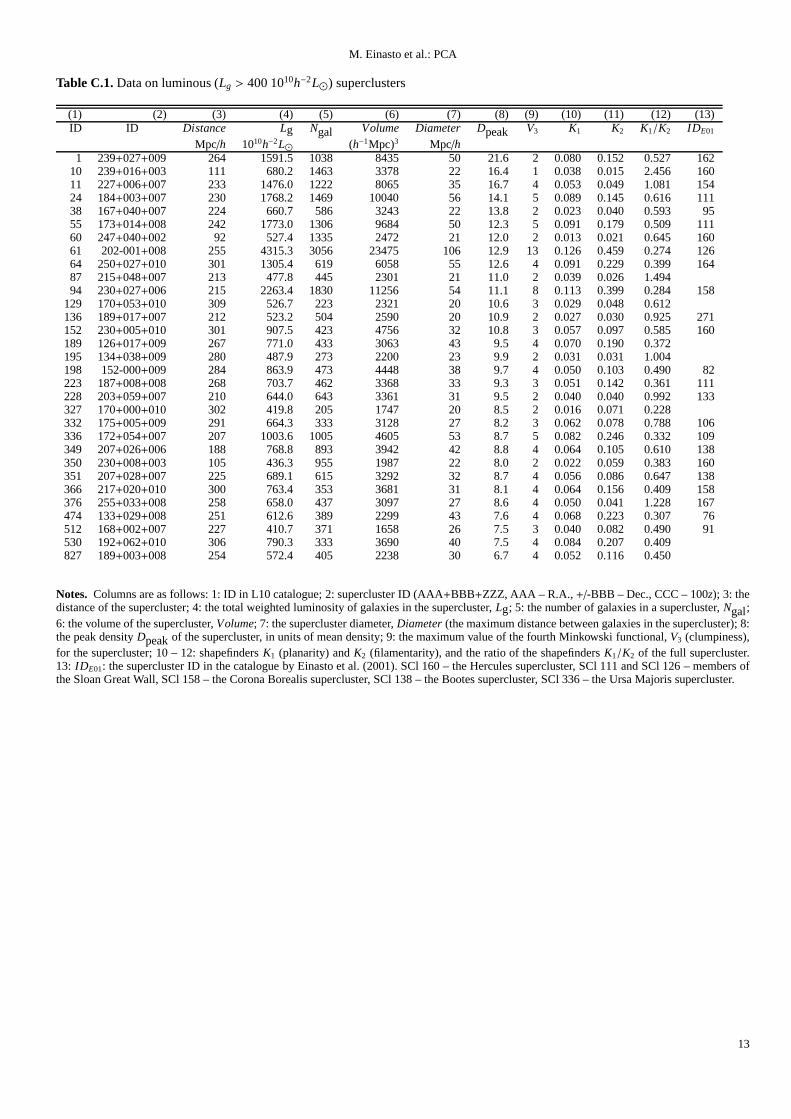
Table C.1. Data on luminous (Lg > 400 1010h−2L⊙) superclusters

(1) (2) (3) (4) (5) (6) (7) (8) (9) (10) (11) (12) (13)ID ID Distance Lg Ngal Volume Diameter Dpeak V3 K1 K2 K1/K2 IDE01

Mpc/h 1010h−2L⊙ (h−1Mpc)3 Mpc/h1 239+027+009 264 1591.5 1038 8435 50 21.6 2 0.080 0.152 0.527 162

10 239+016+003 111 680.2 1463 3378 22 16.4 1 0.038 0.015 2.456 16011 227+006+007 233 1476.0 1222 8065 35 16.7 4 0.053 0.049 1.081 15424 184+003+007 230 1768.2 1469 10040 56 14.1 5 0.089 0.145 0.616 11138 167+040+007 224 660.7 586 3243 22 13.8 2 0.023 0.040 0.593 9555 173+014+008 242 1773.0 1306 9684 50 12.3 5 0.091 0.179 0.509 11160 247+040+002 92 527.4 1335 2472 21 12.0 2 0.013 0.021 0.645 16061 202-001+008 255 4315.3 3056 23475 106 12.9 13 0.126 0.459 0.274 12664 250+027+010 301 1305.4 619 6058 55 12.6 4 0.091 0.229 0.399 16487 215+048+007 213 477.8 445 2301 21 11.0 2 0.039 0.026 1.49494 230+027+006 215 2263.4 1830 11256 54 11.1 8 0.113 0.399 0.284 158

129 170+053+010 309 526.7 223 2321 20 10.6 3 0.029 0.048 0.612136 189+017+007 212 523.2 504 2590 20 10.9 2 0.027 0.030 0.925 271152 230+005+010 301 907.5 423 4756 32 10.8 3 0.057 0.097 0.585 160189 126+017+009 267 771.0 433 3063 43 9.5 4 0.070 0.190 0.372195 134+038+009 280 487.9 273 2200 23 9.9 2 0.031 0.031 1.004198 152-000+009 284 863.9 473 4448 38 9.7 4 0.050 0.103 0.490 82223 187+008+008 268 703.7 462 3368 33 9.3 3 0.051 0.142 0.361 111228 203+059+007 210 644.0 643 3361 31 9.5 2 0.040 0.040 0.992 133327 170+000+010 302 419.8 205 1747 20 8.5 2 0.016 0.071 0.228332 175+005+009 291 664.3 333 3128 27 8.2 3 0.062 0.078 0.788 106336 172+054+007 207 1003.6 1005 4605 53 8.7 5 0.082 0.246 0.332 109349 207+026+006 188 768.8 893 3942 42 8.8 4 0.064 0.105 0.610 138350 230+008+003 105 436.3 955 1987 22 8.0 2 0.022 0.059 0.383 160351 207+028+007 225 689.1 615 3292 32 8.7 4 0.056 0.086 0.647 138366 217+020+010 300 763.4 353 3681 31 8.1 4 0.064 0.156 0.409 158376 255+033+008 258 658.0 437 3097 27 8.6 4 0.050 0.041 1.228 167474 133+029+008 251 612.6 389 2299 43 7.6 4 0.068 0.223 0.307 76512 168+002+007 227 410.7 371 1658 26 7.5 3 0.040 0.082 0.490 91530 192+062+010 306 790.3 333 3690 40 7.5 4 0.084 0.207 0.409827 189+003+008 254 572.4 405 2238 30 6.7 4 0.052 0.116 0.450

Notes. Columns are as follows: 1: ID in L10 catalogue; 2: supercluster ID (AAA+BBB+ZZZ, AAA – R.A., +/-BBB – Dec., CCC – 100z); 3: thedistance of the supercluster; 4: the total weighted luminosity of galaxies in the supercluster,Lg; 5: the number of galaxies in a supercluster,Ngal;6: the volume of the supercluster,Volume; 7: the supercluster diameter,Diameter (the maximum distance between galaxies in the supercluster); 8:the peak densityDpeakof the supercluster, in units of mean density; 9: the maximumvalue of the fourth Minkowski functional,V3 (clumpiness),for the supercluster; 10 – 12: shapefindersK1 (planarity) andK2 (filamentarity), and the ratio of the shapefindersK1/K2 of the full supercluster.13: IDE01: the supercluster ID in the catalogue by Einasto et al. (2001). SCl 160 – the Hercules supercluster, SCl 111 and SCl 126 – members ofthe Sloan Great Wall, SCl 158 – the Corona Borealis supercluster, SCl 138 – the Bootes supercluster, SCl 336 – the Ursa Majoris supercluster.

13