scribe notes proof complexity
TRANSCRIPT
Scribe Notes
Proof ComplexityMath 267A - UCSD, Winter 2002
Instructor: Sam Buss
1

Math 267a - Propositional Proof Complexity Table of Contents
Contents
Lecture #1, Robert Ellis 4
1 Introduction to Propositional Logic 4
2 Propositional Proof Systems 6
Lecture #2, Sashka Davis 10
3 Introduction to Frege Proof Systems 10
4 The Completeness and Implicational Completeness Theorems 12
5 Observations 13
6 P-simulate 13
Lecture #3, Reid Andersen 15
7 p-Simulation 15
8 Extended Frege Sytems 16
Lecture #4, Alan Nash 17
9 The Unification Problem 17
10 Extended Frege Systems (Again) 18
Lecture #5, Tamsen Dunn 20
11 The Pigeon Hole Principle 20
12 Tree-Like versus Non-Tree-Like Proofs 22
Lecture #6, Rosalie Iemhoff 24
13 Substitution Frege systems 24
14 The best known lower bounds on proof lengths 26
15 Resolution 27
2

Math 267a - Propositional Proof Complexity Table of Contents
Lecture #7, Dan Curtis 29
16 Completeness and Soundness of Resolution Proofs 29
Lecture #8, Bryant Forsgren 33
17 Last Time 33
18 Views of Resolution Refutations 33
19 Exponential Lower Bounds on Refutation Proofs of the Pigeon Hole Principle 34
Lecture #9, Nathan Segerlind 37
20 Last Time 37
21 A Size Lower Bound for Resolution Refutations of PHPn+1n 37
22 Lower Bounds for Resolution Proofs of Circuit Lower Bounds 40
Lecture #10, Scribe notes not available. 40
Lecture #11, Liz Arentzen 41
23 Monotone Craig Interpolation 41
Bibliographic citations. 45
3

Math 267a - Propositional Proof Complexity Lecture #1: 14 January 2002
Math 267a - Propositional Proof Complexity
Lecture #1: 14 January 2002
Lecturer: Sam Buss
Scribe Notes by: Robert Ellis
1 Introduction to Propositional Logic
1.1 Symbols and Definitions
The language of propositional logic consists of connectives, propositional variables, parentheses andformulas, shown in the table below. The meanings of the symbols are given by their corresponding
connectives ∨,∧,¬,→variables x1, x2, . . .parentheses (, )formulas (φ ∧ ψ), (φ ∨ ψ), (φ → ψ), (¬φ), etc.
Table 1: Components of Statements of Propositional Logic
truth tables. The ∨ (“logical or”), ∧ (“logical and”) and → (“logical implication”) operators arebinary, while the ¬ (“logical negation”) operator is unary. The truth tables for these operatorsare constructed by exhaustively assigning all possible truth values to the variables and listing theresult defined by the operator.
x1 x2 x1 ∨ x2
T T TT F TF T TF F F
x1 x2 x1 ∧ x2
T T TT F FF T FF F F
x1 x2 x1 → x2
T T TT F FF T TF F T
x1 ¬x1
T FF T
A truth assignmentτ : x1, x2, . . . → T, F
assigns logical truth values to the variables. A truth assignment τ extends to a truth assignmentτ : φ → T, F on the set of formulas φ by assigning truth values to variables in the formulaand determining the truth of the formula by invoking the definitions of the connectives. The truthof a compound formula depends on the truth of its constituents. For example,
τ(φ → ψ) =
T if τ(φ) =F or τ(ψ) =TF otherwise.
4

Math 267a - Propositional Proof Complexity Lecture #1: 14 January 2002
Two other common symbols, ⊕ and |, are the “exclusive or” and “nand” binary operatorsexpressible in terms of the first four symbols. Specifically, x1|x2 := ¬(x1 ∧ x2) and x1 ⊕ x2 :=¬((x1 ∧ x2) ∨ (x1|x2)).
1.2 SAT, TAUT, P and NPStatements in propositional logic, or predicates, which are of special interest are those for whichthere exists a truth assignment for which the predicate is true, and those for which the predicateis true for all truth assignments.
Definition The predicate φ is a tautology if for all truth assignments τ , τ(φ) = T.
Definition The predicate φ is satisfiable if there exists a truth assignment τ such that τ(φ) = T.
Based on their definitions, tautologies and satisfiable predicates are related as follows.
Fact If φ is a tautology then (¬φ) is not satisfiable.
Definition TAUT is the set of all tautologies.
Definition SAT is the set of all satisfiable formulas.
The problem of recognizing a member of SAT is fundamental in computational complexity. Pis defined to be the set of all predicates that are polynomial time recognizable. In this context,a predicate is a decision procedure yielding either ‘T’ or ‘F’. Polynomial time recognizable meansthere exists an algorithm implementing the decision procedure which is bounded in the number ofsteps by a polynomial in the size of the input.
Example Let WFF, the set of well-formed formulas, be defined as the set of strings which arevalidly formed formulas build on connectives, parentheses and variables. Then the predicate WFFis a member of P.
Definition NP is the set of predicates Q which can be expressed as
Q(x) = (∃y, |y| < p(|x|))R(x, y),
where p is a polynomial, |x| is the length of x viewed as a string, y is the “witness” to x, and R isa polynomial time algorithm which verifies that y is a witness to x. Thus Q(x) = T if and only ifa witness y exists such that the time property R(x, y) holds.
To show that SAT is in NP, simply express it in the above form; e.g.,
SAT (X) ≡ (∃y, (|y| ≤ |x|))TRU(x, y),
where TRU(x, y) is the algorithm which verifies that y encodes a truth assignment which satisfiesx. We may take y to be weakly less than x in length, because it can simply encode truth values ofthe variables in the formula x as binary digits.
Homework 1 Turn in a proof of P = NP or P 6= NP for $1,000,000 (from the Clay MathematicsInstitute) and an A+.
5

Math 267a - Propositional Proof Complexity Lecture #1: 14 January 2002
2 Propositional Proof Systems
One purpose of propositional proof systems is to provide evidence of the membership of a formulaφ in the set of tautologies TAUT. Of particular interest is the size of the proof of a tautology.
2.1 Truth Tables
Truth tables provide straightforward but lengthy verifications of tautologies. The proof of a tautol-ogy proceeds by exhaustively writing down all 2n truth assignments for a predicate in n variables,and resolving the truth in each case by the logical rules. The written-out truth table is the actualproof. A proof of the tautology A → (B → A) is given by the following table.
A B B → A A → (B → A)T T T TT F T TF T F TF F T T
We can easily obtain an estimate for the size of a truth table proof for a tautology φ. Letp be the number of distinct variables, and let m be the total number of unary or binary logicaloperators. The the truth table has approximately m2p = 2O(p) entries. The size of such a table forp = 100 would be at least 1000 times the age of the universe in nanoseconds.
The exponential growth rate of the size of the truth table makes this kind of proof infeasiblefor even relatively small numbers of variables. Growth rates like 2n, 2εn and 2nε
are all “too big”in this sense. We prefer growth rates like n, n log n, n2 and n3, which are feasible for large valuesof n.
2.2 Frege Proof Systems
A Frege Proof System consists of axioms, substitution rules and a rule of inference from which alltautologies can be proved in a much more tractable form that that of truth tables. Informally, aproof of a formula φ consists of a sequence of formulas in which each step is either an axiom, asubstitution of a previous step, or derived by inference, and the last step is φ.
2.2.1 Proof System Components
We formalize these notions in the following definitions.
Definition The schematic axiom of a Frege proof system are a list of tautologies called schematictautologies which may be used as the starting point of a Frege proof.
The list of schematic tautologies in a common Frege proof system, which allows any tautologyto be proved, appears in Table 2. Here, A, B and C are variables, and for well-definedness ofassociativity we adopt the shorthand φ → ψ → χ := φ → (ψ → χ).
6

Math 267a - Propositional Proof Complexity Lecture #1: 14 January 2002
A → (B → A) A ∧ B → B(A → B) → (A → B → C) → (A → C) A ∧ B → AA → A ∨ B A → B → A ∧ BB → A ∨ B (A → B) → (A → ¬B) → ¬A(A → C) → (B → C) → (A ∨ B → C) ¬¬A → A
Table 2: Schematic Tautologies for a Frege proof system
Definition A schematic substitution σ is a mapping σ : V → WFF from a set V ⊆ x1, x2, . . .of variables to the set of well-formed formulas, written by
σ = (x1/φ1, . . . , xk/φk),
where φi = σ(xi) = xiσ.
Informally, a schematic substitution σ replaces a variable xi with some formula φi.
Definition Aσ is defined to be the result of replacing (simultaneously) each occurrence of xi inthe formula A by xiσ = σ(xi).
Example Let A = x1 → x2 and let σ = (x1/(x1 ∧ x2), x2/x1). Then
Aσ = (x1 ∧ x2) → x1.
Fact If φ ∈ TAUT , then for all σ, φσ ∈ TAUT .
Definition The schematic rule of inference called modus ponens, or MP, is represented by
x1 x1 → x2
x2,
and is invoked by confirming that x2 is true whenever x1 is true and x1 implies x2.
Definition A schematic inference, denoted
A1, . . . , Ak
B,
means that for all σ, if A1σ, . . . , Akσ have been proved, then Bσ can be inferred. Taking k = 0yields a schematic axiom.
The above definitions are used to develop a schematic proof that some formula φ is a tautology.We formalize this type of Frege proof as follows.
Definition An F0-proof is a sequence of formulas φ1, φ2, . . . , φk such that each φi is either anaxiom or is inferred by modus ponens from some φj and φl, for j, l < i. It is called a proof of φk.
7

Math 267a - Propositional Proof Complexity Lecture #1: 14 January 2002
2.2.2 Proof System Characteristics
In the Frege proof system just described, the properties of soundness and completeness are highlydesirable. Soundness means that no proof exists for a formula that is not a tautology. Completenessmeans that every tautology has a corresponding proof. We introduce the symbolism F0
φ to denotethat F0 is a proof of φ, and use |= φ to denote φ ∈ TAUT .
Theorem 1 (Soundness) If F0φ then φ ∈ TAUT .
Proof The proof is by induction on the number of steps in the F0 proof. The proof starts with aschematic axiom which is a tautology, every step in the proof by substitution is a tautology, andMP preserves tautologies, and so φ is a tautology.
Theorem 2 (Completeness) If φ ∈ TAUT , then F0φ for some proof F0.
Proof The proof of completeness for this Frege proof system is deferred until Lecture #2.
Generally, we require an expanded notion of soundness and completeness than what is outlinedabove. In particular, we may wish to prove a tautology in a proof system starting from an extraset of axiomatically tautological formulas.
Definition Let Γ be a set of formulas. Then Γ |= φ provided that for all truth assignments τ , iffor all γ ∈ Γ we have τ(γ) = T, then τ(φ) = T. We call Γ |= φ a tautological implication.
The corresponding version of a F0-proof is as follows.
Definition Let Γ be a set of formulas. Then Γ F0φ provided there exists a sequence φ1, . . . , φk = φ
such that each φi is in Γ or is an (instance of an) axiom or is inferred by MP. We call the sequencean F0-proof with hypotheses.
We would certainly like to know how to deal with implicational tautologies when Γ is an infiniteset. Fortunately, a compactness result simplifies things.
Theorem 3 (Compactness of tautological implication) If Γ |= φ, then there exists a finitesubset Γ0 ⊆ Γ such that Γ0 |= φ.
Proof The proof is left as an exercise.
Proposition 4 (Derived substitution rule)
1. If F0A and σ is a substitution, then F0
Aσ.
2. If Γ F0φ, then Γσ F0
φσ.
Proof Part 1 proceeds by applying σ to the whole F0-proof. Start with the sequence φ1, φ2, . . . , φk =A and replace φi with φiσ to obtain φ1σ, φ2σ, . . . , φkσ = Aσ. Part 2 proceeds similarly.
8

Math 267a - Propositional Proof Complexity Lecture #1: 14 January 2002
Note that a double substitution into a schematic axiom, such as φi replaced with φiσ can besimplified to a single substitution. Define
σ : xi 7→ xiσ = φi, andτ : xi 7→ xiτ = ψi.
Then the double substitution (Aσ)τ) can be written as A(στ) since
(στ) : xi 7→ φiτ = xiστ.
The implicational soundness and completeness theorems are as follows.
Theorem 5 (Implicational soundness of F0) If Γ F0φ, then Γ |= φ.
Proof The proof proceeds by induction on the number of steps in the F0-proof.
Theorem 6 (Implicational completeness of F0) If Γ |= φ, then Γ F0φ.
Proof The proof is deferred until Lecture #2.
9
Math 267a - Propositional Proof Complexity Lecture #2: 16 January 2002
Math 267a - Propositional Proof Complexity
Lecture #2: 16 January 2002
Lecturer: Sam Buss
Scribe Notes by: Sashka Davis
3 Introduction to Frege Proof Systems
Last time we stated the Completeness and the Soundness theorems for the Frege Proof Systems,today we focus on the Completeness Theorem. The main point of the Completeness Theorem isthat there exists a Frege Proof System which is complete.
We begin with an example of F0-proof. The axioms of the Frege system we will use, are theSchematic Tautologies, defined in the previous lecture (Ax1 denoting the first axiom, Ax2 thesecond, etc.).
Example (A → A) has an F0-proof.
ProofThe following five lines form an F0-proof of (A → A).
A → (A→A) → A, an instance of axiom Ax1A → A → A, an instance of axiom Ax1(A→(A→A)) → (A→(A→A)→A)) → (A→A), an instance of axiom Ax2(A → (A→A) → A) → (A→A), by MPA→A. 2
Proof Complexity The F0-proof has O(1) lines and O(|A|) symbols.
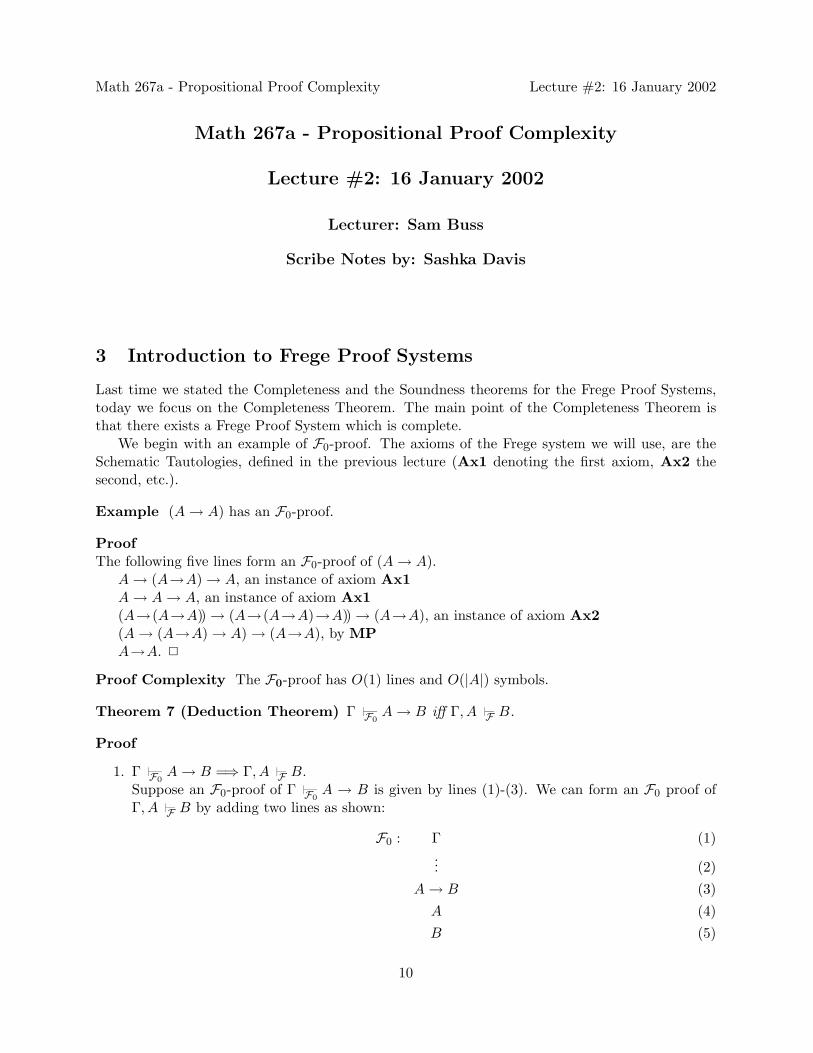
Theorem 7 (Deduction Theorem) Γ F0A → B iff Γ, A F B.
Proof
1. Γ F0A → B =⇒ Γ, A F B.
Suppose an F0-proof of Γ F0A → B is given by lines (1)-(3). We can form an F0 proof of
Γ, A F B by adding two lines as shown:
F0 : Γ (1)... (2)
A → B (3)A (4)B (5)
10

Math 267a - Propositional Proof Complexity Lecture #2: 16 January 2002
Line (4) is the added new hypothesis. Line (5) is derived by MP. Thus we obtain F0-prooffor Γ, A F B.
Proof Complexity O(n) lines and O(nm) symbols.
2. Γ, A F0B =⇒ Γ F A → B.
Proof Idea: Let the F0-proof of Γ, A F0B be a sequence B = ϕ1, . . . , ϕn. We shall use the
substitution rule and replace each ϕi by A→ϕi. The sequence of formulas A→ϕi is not avalid proof, but it can be converted into a valid proof as follows. Each ϕi either is A, or isinferred from A by MP, or is an axiom, or is a member of Γ. Thus to patch the proof weneed to exhaust the following four cases.
• Case 1: ϕi is AThen we re-use the 5-line proof of A→ A.
• Case 2: ϕi is inferred by MP:ϕj ϕk = ϕj → ϕi
ϕi, j, k < i
A → ϕj
A → ϕj → ϕi
(A→ϕj) → (A→(ϕi → ϕj)) → (A → ϕi), by Ax2A → ϕi, by MP.
• Case 3: ϕi is an axiomϕi → (A → ϕi) , by Ax1 .So ϕi can be replaced by the three line proof of A→ϕi.
• Case 4: ϕi ∈ Γϕi → (A → ϕi) , by Ax1 .
2
Proof ComplexityEach line in the original F0-proof becomes either three or five lines in the F0-proof ofΓ F0
A → B. The proof complexity remains O(n) lines and O(nm) symbols.
3.1 Usage of the Deduction Theorem
Let∧∧k
i=1Ai, denotes any parenthesization of the conjunction of A1, . . . , An.
Example Given F0
∧∧ki=1Ai → Ai0, with proof complexity O(k) lines and O(k|B|) symbols,
where B =∧∧k
i=1Ai, prove that∧∧k
i=1Ai F0Ai0.
Proof We follow the F0-proof. Begin with∧∧k
i=1Ai. Repeatedly use the axioms (A ∧ B → B)and (A ∧ B → A) with MP. All the lines are well behaved. 2
11
Math 267a - Propositional Proof Complexity Lecture #2: 16 January 2002
4 The Completeness and Implicational Completeness Theorems
Recall that the Completeness theorem states: φ ∈ TAUT =⇒ F0φ, for some proof F0. Now we
state and prove the Implicational Completeness Theorem.
Theorem 8 (Implicational Completeness Theorem) If Γ |= A then Γ F0 A.
Proof If Γ |= A, then there exists a finite Σ, Σ ⊂ Γ, s.t. Σ |= A. So w.l.o.g. Γ is finite. LetΓ = B1, . . . Bk, then |= B1 → (B2 → (. . . → (Bk → A) . . . )).By the Completeness Theorem there exists an F0-proof of the tautology. By applying the DeductionTheorem k times we obtain Γ F0 A. 2
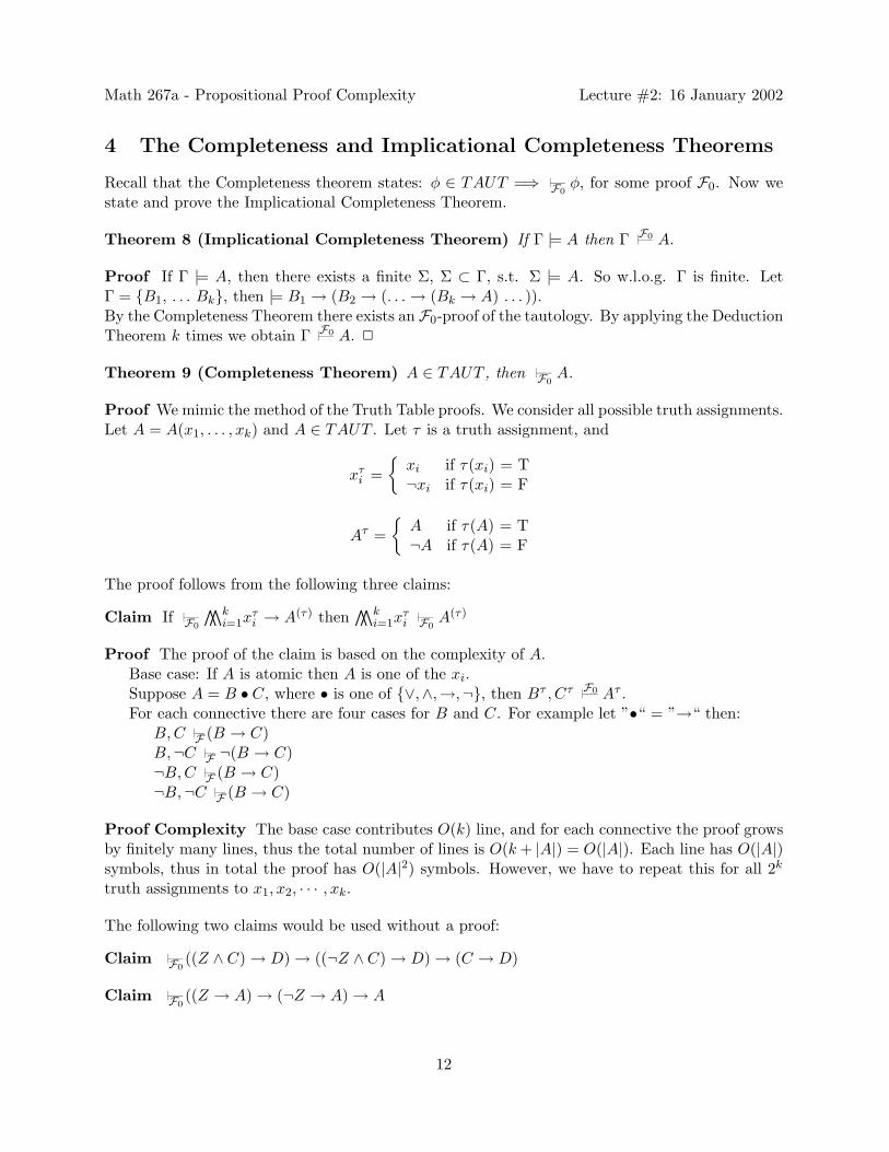
Theorem 9 (Completeness Theorem) A ∈ TAUT , then F0A.
Proof We mimic the method of the Truth Table proofs. We consider all possible truth assignments.Let A = A(x1, . . . , xk) and A ∈ TAUT . Let τ is a truth assignment, and
xτi =
xi if τ(xi) = T¬xi if τ(xi) = F
Aτ =
A if τ(A) = T¬A if τ(A) = F
The proof follows from the following three claims:
Claim If F0
∧∧ki=1x
τi → A(τ) then
∧∧ki=1x
τi F0
A(τ)
Proof The proof of the claim is based on the complexity of A.Base case: If A is atomic then A is one of the xi.Suppose A = B • C, where • is one of ∨,∧,→,¬, then Bτ , Cτ F0 Aτ .For each connective there are four cases for B and C. For example let ”•“ = ”→“ then:
B, C F (B → C)B,¬C F ¬(B → C)¬B, C F (B → C)¬B,¬C F (B → C)
Proof Complexity The base case contributes O(k) line, and for each connective the proof growsby finitely many lines, thus the total number of lines is O(k + |A|) = O(|A|). Each line has O(|A|)symbols, thus in total the proof has O(|A|2) symbols. However, we have to repeat this for all 2k
truth assignments to x1, x2, · · · , xk.
The following two claims would be used without a proof:
Claim F0((Z ∧ C) → D) → ((¬Z ∧ C) → D) → (C → D)
Claim F0((Z → A) → (¬Z → A) → A
12
Math 267a - Propositional Proof Complexity Lecture #2: 16 January 2002
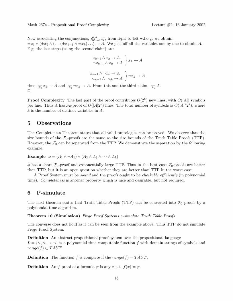
Now associating the conjunctions,∧∧k
i=1xτi , from right to left w.l.o.g. we obtain:
±x1 ∧ (±x2 ∧ (. . . (±xk−1 ∧ ±xk) . . .) → A. We peel off all the variables one by one to obtain A.E.g. the last steps (using the second claim) are:
xk−1 ∧ xk → A¬xk−1 ∧ xk → A
xk → A
xk−1 ∧ ¬xk → A¬xk−1 ∧ ¬xk → A
¬xk → A
thus F0xk → A and F0
¬xk → A. From this and the third claim, F0A.
2
Proof Complexity The last part of the proof contributes O(2k) new lines, with O(|A|) symbolsper line. Thus A has F0-proof of O(|A|2k) lines. The total number of symbols is O(|A|22k), wherek is the number of distinct variables in A.
5 Observations
The Completeness Theorem states that all valid tautologies can be proved. We observe that thesize bounds of the F0-proofs are the same as the size bounds of the Truth Table Proofs (TTP).However, the F0 can be separated from the TTP. We demonstrate the separation by the followingexample.
Example φ = (A1 ∧ ¬A1) ∨ (A2 ∧ A3 ∧ · · · ∧ Ak).
φ has a short F0-proof and exponentially large TTP. Thus in the best case F0-proofs are betterthan TTP, but it is an open question whether they are better than TTP in the worst case.
A Proof System must be sound and the proofs ought to be checkable efficiently (in polynomialtime). Completeness is another property which is nice and desirable, but not required.
6 P-simulate
The next theorem states that Truth Table Proofs (TTP) can be converted into F0 proofs by apolynomial time algorithm.
Theorem 10 (Simulation) Frege Proof Systems p-simulate Truth Table Proofs.
The converse does not hold as it can be seen from the example above. Thus TTP do not simulateFrege Proof System.
Definition An abstract propositional proof system over the propositional languageL = ∨,∧,→,¬ is a polynomial time computable function f with domain strings of symbols andrange(f) ⊂ TAUT .
Definition The function f is complete if the range(f) = TAUT .
Definition An f -proof of a formula ϕ is any x s.t. f(x) = ϕ.
13
Math 267a - Propositional Proof Complexity Lecture #2: 16 January 2002
Definition F0 as an abstract proof system is defined as:
fF0(x) =
ϕ if x codes a valid F0-proof of ϕ(x1 ∨ ¬x1) otherwise
This idea for constructing an abstract proof systems works for many other proof systems too. Forexample, let ZF be the usual theory of set theory, then
fZF (x) =
ϕ if x codes a valid ZF proof of ”ϕ is a tautology“(x1 ∨ ¬x1) otherwise
is an abstract proof system.
14

Math 267a - Propositional Proof Complexity Lecture #3: 23 January 2002
Math 267a - Propositional Proof Complexity
Lecture #3: 23 January 2002
Lecturer: Sam Buss
Scribe Notes by: Reid Andersen
7 p-Simulation
Definition Let f and g be proof systems in the same language. We say f p-simulates g if thereexists a poly-time computable function H(x) such that ∀x, g(x) = f(H(x)). We say f simulates gif there exists a polynomial p(n) such that ∀x∃y, |y| ≤ p(|x|) and f(y) = g(x).
Definition A proof system f is maximal if f simulates g for any proof system g. A proof systemf is super if there exists a polynomial p(n) such that ∀ϕ ∈ TAUT , ∃x such that |x| ≤ p(|ϕ|) andf(x) = ϕ. Note that any super proof system is maximal.
Open Question Is there a super or maximal proof system?
Theorem 11 [3] [Cook] There exists a super proof system ⇐⇒ NP = co − NP .
Homework 2 Prove the above theorem for a homework excercise.
Definition A Frege system is a proof system given by a finite set of of schematic axioms andinference rules, and must be implicationally sound and implicationally complete.
Theorem 12 [4] [Cook-Reckhow] If F1, F2 are Frege systems, then F1 p-simulates F2.
Proof For the proof we will assume F1 and F2 have the same language, but the statement istrue in general. Consider a rule of F2, A1...Ak
B . F1 can prove A1 . . . Ak ` B by the implicationalcompleteness of Frege proof systems. Consider an F2-proof ϕ1 . . . ϕn. We convert to an F1-proofas follows: ϕi follows from an inference rule A1σ...Akσ
Bσ , where A1σ = ϕi1 , . . . , Akσ = ϕik , withi1 . . . ik < i, and Bσ = ϕi. Assuming ϕi1 . . . ϕik already proved, use the substitution σ on theF1-proof A1 . . . Ak ` B to get an F1-proof ϕi1 . . . ϕik ` ϕi. Combining this proof and the proof ofϕi1 . . . ϕik yields an F1-proof of φi.
Proof Complexity This is a polynomial time procedure. For each line of the F2-proof, thereare O(1) lines in the F1-proof. If the F2 proof has n lines and m total symbols, the F1 proof hasO(n) lines, and each line has O(m) symbols. So the F1-proof contains O(n) lines, and O(mn)total symbols. Since n ≤ m, the size of the F1-proof is bounded by a polynomial in the size of theF2-proof.
15

Math 267a - Propositional Proof Complexity Lecture #3: 23 January 2002
Open Question Can the bound of O(mn) symbols in the preceeding proof be improved to O(m)?It can if we assume that F1 has modus ponens, but is it true in general?
Open Question Are Frege systems super? or maximal?
Open Question Is there a “natural” proof system stronger than Frege systems?
8 Extended Frege Sytems
Definition Here we define an extended Frege system, eF . An eF0-proof is the same as an F0-proof, except the size of the proof is computed differently. The size of an extended Frege proof ofA is (# of lines in the proof) + |A|.
Example In a previous lecture we saw that any formula A → A has an F0-proof of five lines. Sothere is an eF0-proof of A → A of size 5 + |A|.
The catch is that an extended Frege system as defined above is not an abstract proof system,since an abstract proof system defines the size of a proof x to be the number of symbols in x. Forthis reason we will present an encoding where an eF0 proof with size n in the extended Frege sensecan be encoded by a string of length O(poly(n)). We also present a polynomial time decodingalgorithm to verify that a string encodes a valid eF0 proof. This decoding algorithm defines anabstract proof system with the notion of size that we desire, within a polynomial.
Encoding [7] [Parikh] Number the rules of inference. The axioms take values 0...9, and modusponens takes 10. We represent an eF0-proof ϕ1, . . . , ϕn = ϕ by a tuple 〈e1, . . . , en, ϕ〉 where ifϕi is an instance of axiom k then ei = k, and if ϕi is inferred from ϕji , ϕki by modus ponens,ei = 〈10, ji, ki〉.
The size of this proof skeleton is O(nlogn + |ϕ|), where n is the size of the eF0 proof.
Claim There is a polynomial time algorithm to decide if an encoding corresponds to a valideF0-proof.
Proof We convert the skeleton into a unification problem which has a solution iff the proof skeletonis valid. We create new “metavariables” y1...yn, and zi
j , and search for a substitution σ : yi 7→ ϕi
which must satisfy the following equations:
1. yn.= ϕ. (means σyn = ϕ)
2. if ei = 〈10, ji, ki〉, we require that yki
.= (yji → yi)
3. for 0 ≤ ei ≤ 9 let A be the ei-th axiom. Replace each xj in A by zij , and denote this instance
of the axiom A by Ai. We require that yi.= Ai.
A substitution σ that satisfies these requirements is called a unifier, and the encoding corre-sponds to a valid eF0-proof of ϕ if and only if such a σ exists. More on this next time.
16

Math 267a - Propositional Proof Complexity Lecture #4: 28 January 2002
Math 267a - Propositional Proof Complexity
Lecture #4: 28 January 2002
Lecturer: Sam Buss
Scribe Notes by: Alan Nash
9 The Unification Problem
9.1 The Problem
Last time we looked at how to solve the system: x = φ, φ = ψ → x. In general, given:
• Variables: x, y, z, . . .
• Function Symbols: f, g, h, . . ., each with specified arity (including constants as 0-ary func-tions)
• Terms: built from variables and function symbols
• Finite sets of equations: si=ti (where si, ti are terms)
the unification problem is to find a substitution σ such that siσ = tiσ where equality here is equalityof symbols.
Example Take the system with a single binary function symbol f and equations:
x1 = f(x2, x2)x2 = f(x3, x3)x3 = f(x4, x4)
a solution is given by σ such that:
σ(x3) = f(x4, x4)σ(x2) = f(f(x4, x4), f(x4, x4))σ(x1) = f(f(f(x4, x4), f(x4, x4)), f(f(x4, x4), f(x4, x4)))
As this example shows, in the worst case the solution’s size is exponential in the size of theproblem (total number of symbols to represent it).
Example The system with the single equation f(x1, x2) = g(x1, x2) is unsolvable: the functionsymbols clash.
Example The system with equations x=g(y) and y=h(x) is unsolvable (the solution must befinite): it yields the derived equation x=g(h(x)) (“occurs check”).
We will see that these are the only two kinds of things that can go wrong.
17
Math 267a - Propositional Proof Complexity Lecture #4: 28 January 2002
9.2 An Algorithm for the Unification Problem
First, notice that terms can be represented by ordered directed acyclic diagrams (ODAGs). By‘ordered’ we mean that there is a total ordering on each set of edges coming out of a vertex. Whenrepresented as ODAGs, the solutions are always polynomial in size.
To solve an unification problem, we first define an equivalence relation ≈ on terms, as follows:
1. s=t → s ≈ t (equation in system)
2. s = t → s ≈ t (equal as strings)
3. f(s1, s2, . . . , sk) ≈ f(t1, t2, . . . , tk) → ∀i(si ≈ ti)
4. s ≈ t → t ≈ s
5. r ≈ s ≈ t → r ≈ t
Example Given the system f(x, g(y))=f(h(y), z) we have x ≈ h(y) and z ≈ g(y)
Claim A unification problem is solvable iff (a) There are no r ≈ s so that r and s have differentprincipal (outermost) function symbols and (b) The ≈-equivalence classes are well-ordered (i.e. nocycles) under the extension of the proper subterm relation to the equivalence classes (i.e., [r] ≺ [s]iff r is a proper subterm of s)
Proof: [⇒] suppose that σ is a solution. Then it is easy to show that r ≈ s implies rσ = sσholds, by induction on the cases defining ≈. Similarly, the relation “rσ is a proper subterm of sσ”is a well-ordering that refines r ≺ s.
[⇐] Define σ by induction along ≺ as follows. The base elements are of the form [x], containingonly variables and at most a single constant c. If c ∈ [x] then define σ(x) = c. Otherwise, defineσ(x) = y where y is a new variable that depends only on [x].
For the rest, i.e. x ∈ [f(s1, . . . , sk)] define σ(x) = (f(s1, . . . , sk))σ = f(s1σ, . . . , skσ).Subclaim: v ≈ s implies rσ = sσ (almost immediate).Partial proof: Suppose r = f(r1, . . . , rk) and s = f(s1, . . . , sk). Then by the induction hypoth-
esis, we have riσ = siσ.What we have just described is a polynomial time algorithm. We can obtain the transitive
closure using, for example, a breadth-first search or some other similar means (linear in size ofgraph). In fact, it is quadratic time. Notice that we have considered so far the decision problem;to provide an output in polynomial time we must output ODAGs.
supply reference: Paterson and Wegman provide a linear-time algorithm.To unify a set of terms r, s, t, . . . means to unify the set r=s, s=t, . . .. Conversely, to unify
ri=si : 1 ≤ i ≤ k is the same as to unify f(r1, r2, . . . , rk) = f(s1, s2, . . . , sk)
10 Extended Frege Systems (Again)
Now we look at an alternative definition of extended Frege systems (eF-systems). An eF-systemis a Frege system (F-system) augmented by the extension rule. That is, an eF-proof consists offormulas φ1, . . . , φn where each φi is:
18

Math 267a - Propositional Proof Complexity Lecture #4: 28 January 2002
• an axiom
• inferred by a rule from previous formulas
• is z ↔ ψ where
– z does not occur in ψ,
– z does not occur in any previous line of the proof, and
– z does not occur in φn.
To convert an eF-proof into a F-proof, proceed as follows:
• Replace z by φ wherever z occurs
• Replace ψ ↔ ψ with a F-proof of it (O(1) lines).
Theorem 13 (Statman [8]) An n-line F-proof of φ can be converted into an eFproof of φ withO(n + |φ|) lines and O(n + |φ|2) symbols.
Theorem 14 Any two eF-systems p-simulate each other
Conjecture 1 F-systems do not simulate eF-systems
Notice that in polynomial-size F-proofs, each line is a polynomial-size formula, while in polynomial-size eF-proofs, each line is equivalent to a polynomial-size circuit. This converts to circuits; everyuse of resolution defines a circuit that is then used as input to subsequent circuits: ψ(x1, . . . , xk, z1, . . . , z`)where zi ↔ χi(x1, . . . , xk, zi, . . . , zi−1).
Open Problem Polynomial size formulas have the same expressive power as polynomial circuits
Not only we do not know whether F systems simulate eF systems and whether p-size formulassimulate p-size circuits, we also do not know how to prove either one of this implications if theother one holds.
Proof Nonuniform Uniform BoundedSystem Complexity Complexity ArithmeticF p-size formulas ALOGTIME TNC1
eF p-size circuits P PV/S12
For references on this table, see Steve Cook’s slides from the Edinburgh Complexity Workshop,October 2001, available at
http://www.cs.toronto.edu/ sacook/edinburgh.ps
19

Math 267a - Propositional Proof Complexity Lecture #5: 29 January 2002
Math 267a - Propositional Proof Complexity
Lecture #5: 29 January 2002
Lecturer: Sam Buss
Scribe Notes by: Tamsen Dunn
11 The Pigeon Hole Principle
Last time we finished our introduction to Frege Proof Systems. In this lecture we will give apropositional formulation of and a proof of the Pigeon Hole Principle. Its an interesting side notethat this theorem was considered self evident until it was brought under the scrutiny of discretemathematicians. Now the Pigeon Hole Principle is considered quite subtle. We will begin byanalyzing the familiar form of the theorem.
11.1 The Familiar Form of the Pigeon Hole Principle
Theorem 15 (Pigeon Hole Principle A)
PHPn+1n : ∀n ∈ N¬∃f : 1, 2, ..., n + 1 → 1, 2, ..., n
The above formulation of the Pigeon Hole Principle is sometimes taken in and of itself as thedefinition of n being finite.
11.2 The Pigeon Hole Principle by Induction
Now, we want to write the Pigeon Hole Principle as a family of propositional tautologies. Fix n ≥ 1and let our variables be Pi,j , where 1 ≤ i ≤ n + 1 and 1 ≤ j ≤ n and Pi,j means f(i) = j. In thisway, we no longer have a set of ordered pairs but a set of graphs.
Theorem 16 (Pigeon Hole Principle B)
PHPn+1n :
n+1∧∧i=1
n∨∨j=1
Pi,j →n∧∧
i=1
n+1∧∧j=i+1
n∧∧m=1
(Pi,m ∧ Pj,m)
This ought to be a tautology. Let’s check:
Example [PHP 21 :] (P1,1 ∨ P1,2) → (P1,1 ∨ P2,1 )
So that works. Now for n = 2.
20
Math 267a - Propositional Proof Complexity Lecture #5: 29 January 2002
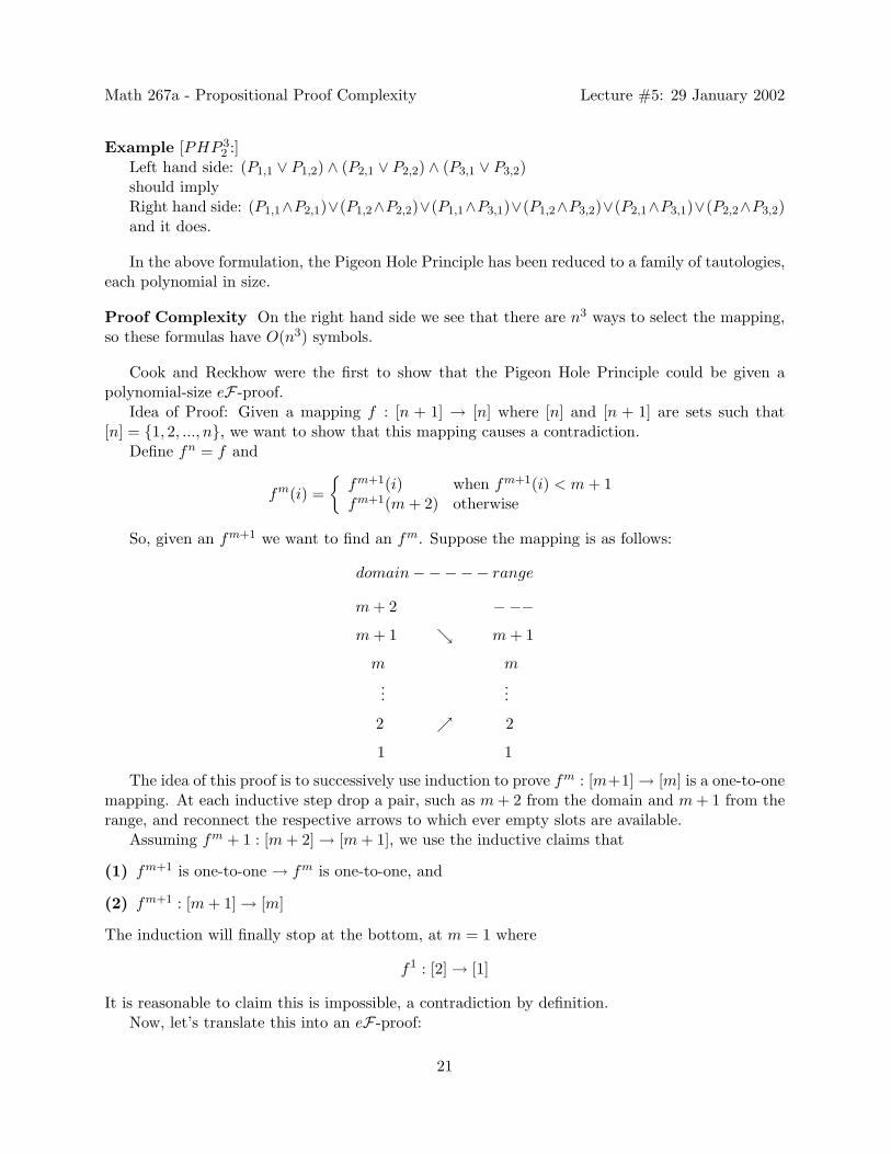
Example [PHP 32 :]
Left hand side: (P1,1 ∨ P1,2) ∧ (P2,1 ∨ P2,2) ∧ (P3,1 ∨ P3,2)should implyRight hand side: (P1,1∧P2,1)∨(P1,2∧P2,2)∨(P1,1∧P3,1)∨(P1,2∧P3,2)∨(P2,1∧P3,1)∨(P2,2∧P3,2)and it does.
In the above formulation, the Pigeon Hole Principle has been reduced to a family of tautologies,each polynomial in size.
Proof Complexity On the right hand side we see that there are n3 ways to select the mapping,so these formulas have O(n3) symbols.
Cook and Reckhow were the first to show that the Pigeon Hole Principle could be given apolynomial-size eF-proof.
Idea of Proof: Given a mapping f : [n + 1] → [n] where [n] and [n + 1] are sets such that[n] = 1, 2, ..., n, we want to show that this mapping causes a contradiction.
Define fn = f and
fm(i) =
fm+1(i) when fm+1(i) < m + 1fm+1(m + 2) otherwise
So, given an fm+1 we want to find an fm. Suppose the mapping is as follows:
domain −−−−− range
m + 2 −−−m + 1 m + 1
m m
......
2 2
1 1
The idea of this proof is to successively use induction to prove fm : [m+1] → [m] is a one-to-onemapping. At each inductive step drop a pair, such as m + 2 from the domain and m + 1 from therange, and reconnect the respective arrows to which ever empty slots are available.
Assuming fm + 1 : [m + 2] → [m + 1], we use the inductive claims that
(1) fm+1 is one-to-one → fm is one-to-one, and
(2) fm+1 : [m + 1] → [m]
The induction will finally stop at the bottom, at m = 1 where
f1 : [2] → [1]
It is reasonable to claim this is impossible, a contradiction by definition.Now, let’s translate this into an eF-proof:
21

Math 267a - Propositional Proof Complexity Lecture #5: 29 January 2002
11.3 eF-Proof of the Pigeon Hole Principle
ProofIdea of Proof: We begin by presuming the hypothesis ¬PHPn+1
n . Then we derive some instanceof ¬PHP 2
1 which can be disproved, and allow that to negate the hypothesis.First introduce some new variables: For ¬PHPn+1
n , we need to have at least the set of Pi,jvariables.
Define ¬PHPm+1m (qm) to have new variables qm
i,j for m = n, ..., 2, 1. Let qni,j ↔ Pi,j . Now the
extension rule is used to introduce qmi,j by
qmi,j ↔ (qm+1
i,j ∨ (qm+1i,m+1 ∧ qm+1
m+2,j))
where 1 ≤ i ≤ m + 1, and 1 ≤ j ≤ m. Since each qm is so defined by the previous qm+1, they areallowed by the extension rule.
Now we claim that eF has polynomial size proofs of ¬PHPm+2m+1 → ¬PHPm+1
m . Proving thisclaim below is equivalent to proving the main theorem.
¬PHPm+2m+1 (qm+1) → ¬PHPm+1
m (qm)
To finish, we need to give an eF-proof of the conjuncts of ¬PHPm+1m (qm) from the conjuncts
of ¬PHPm+2m+1 (qm+1). This is basically a brute-force case analysis. The idea of the case analysis
comes back to the picture we drew earlier. Its simply not possible to map two (or more) elementsof the domain to a single slot in the range. Any time it did would violate one-to-oneness. The fullproof can be found in Cook and Reckhow, JSL 1979.
Proof Complexity All formulas given in this eF-proof are of O(n3) since in the PHP there aren3 steps for that many conjuncts. We step down from n, so that gives us O(n4) lines, and eachline had O(n3) symbols.
Suppose we were instead thinking of an ordinary F-proof. Straightforward conversion failswith exponential blow up. We have to re-express every qi,j in terms of its original variables, thuseliminating all the extension variables from m = n to m = 1. That means we would have roughly3 times as many symbols. For example, qm uses three qm+1 ’s, so by straightforward replacementsubstitution the formulas increase in size by a factor of 3n.
For a different F-proof which is polynomial in size, see Buss, JSL 1978. Buss’s proof rests on acounting argument: “The idea behind the proof is that one can’t [not have the PHP] because thenone set would have more than the other.”
We have very few examples of eF and F size comparisons. However, we still tend to believethe separation is maintained from arguments made in circuit theory. We will come back to this.
12 Tree-Like versus Non-Tree-Like Proofs
Definition A F or eF-proof is tree-like if each formula in the proof is used at most once as ahypothesis of an inference. Other proofs may be dag-like or sequence-like.
Theorem 17 (Krajıcek) Tree-like (extended) F-proofs p-simulate ordinary (extended) F-proofs.
22

Math 267a - Propositional Proof Complexity Lecture #5: 29 January 2002
Intuitively, you might expect the transition to tree-like proofs would cause an an exponentialblow up. But that is not the case.
Proof Given a sequence-like proof, φ1, φ2, ..., φn = φ one wants to create a tree-like proof fromψ1, ψ2, ..., ψn where ψi =
∧∧ij=1 φi . We hope that if multiple formulas are necessary we can use
conjunctions for it once and only once. Now, we claim that the sequence ψ1, ψ2, ..., ψn can be“patched up” to be a tree-like proof. The patching is done by cases:
Case (1) : φi is an axiom.Assume ψi−1 has already been derived. We have the axiom φi. We can derive
ψi−1 → φi → (ψi−1 ∧ φi)
as an instance of A → B → (A ∧ B). So MP twice gave us
ψi−1 ∧ φi
which is equivalent to ψi. And case (1) is proven.Case (2) :φi is inferred from φj and φk by MP. φk is (φj → φi). By assuming we have a proof of ψi−1,
we can complete the rest of the proof by a straightforward unwinding of conjunctions. See theexample below to see how this will work:
Example The following are tautologies: A ∧ B → A and A ∧ B → B, (A → B) ∧ (B → C) →(A → B). Given an instance
(α ∧ β) ∧ γ → (α ∧ β) → α.
(α ∧ β) ∧ γ → (α ∧ β) → ((α ∧ β) → α) → ((α ∧ β) ∧ γ) → α.
Using MP twice, for two conjuncts we have
((α ∧ β) ∧ γ) → α.
Substituting the above equations into our proof, we now have the desired
ψi−1 → φj
andψi−1 → φk
Each of the above is tree like. Now, using a substitution instance of the following tautology:
A → (A → B) → (A → (B → C)) → (A ∧ C)
we can derive from the 3 MP’s that
ψi−1 → (ψi−1 → φj) → (φj−1 → φk) → (ψi−1 ∧ φi)
We are done with case (2) becauseψi−1 ∧ φ = ψi
Therefore, in either case, each ψi can be created for the tree-like proof. That concludes our proofand this lecture.
23

Math 267a - Propositional Proof Complexity Lecture #6: 4 February 2002
Math 267a - Propositional Proof Complexity
Lecture #6: 4 February 2002
Lecturer: Sam Buss
Scribe Notes by: Rosalie Iemhoff
13 Substitution Frege systems
In a previous lecture we encountered certain proof systems for which it is conjectured that they arestronger than Frege systems (in the sense that Frege systems do not p-simulate them). These werethe extended Frege systems. Here we will define other such proof systems: the substitution Fregesystems. We will see that these systems are as strong as extended Frege systems; they p-simulateextended Frege systems and vice versa. As in the case of extended Frege systems, it is an openquestion whether Frege systems p-simulate substitution Frege systems or not.
Definition A substitution Frege system, sF , is a Frege system augmented with a substitution ruleA/Aσ. Thus a proof in a substitution Frege system sF is a sequence ϕ1, . . . , ϕn, where every ϕi isan axiom of F , or inferred from earlier ϕj by a rule of F , or ϕi = ϕjσ, for some j < i and somesubstitution σ.
Note that substitution Frege systems are indeed complete proof systems; it is not difficult to seethat they are sound and complete (the substitution rule is clearly sound, and completeness followsfrom the fact that Frege systems are complete). Note however that they are not implicationallysound. This is not a problem since implicational soundness is not required for a proof system.
Theorem 18 sF-systems and eF-systems p-simulate each other.
Proof We will only show that sF-systems p-simulate eF-systems, the other direction can be foundin [6] or [5] (Lemma 4.5.5). For this proof we consider extended Frege systems of the second type,i.e. with an extension rule. Let ϕ1, . . . , ϕn be a proof in an extended Frege system eF of size k.Thus k = O(n + |ϕn|). W.l.o.g. we can assume that the first m lines in the proof are extensionrules and that the others are not: for i ≤ m, ϕi = zi ↔ χi(x, z1, . . . , zi−1), i.e. ϕi is an instance ofthe extension rule, and for i > m, ϕi is not an instance of the extension rule. Clearly, we have
ϕ1, . . . , ϕm `F ϕn.
Observe that this Frege proof has size at most k. By the Deduction Theorem (Lecture #2) wehave
`F(∧∧m
i=1(zi ↔ χi)
)→ ϕn, (6)
24
Math 267a - Propositional Proof Complexity Lecture #6: 4 February 2002
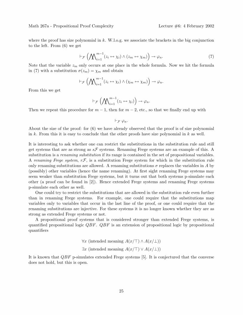
where the proof has size polynomial in k. W.l.o.g. we associate the brackets in the big conjunctionto the left. From (6) we get
`F(∧∧m−1
i=1(zi ↔ χi) ∧ (zm ↔ χm)
)→ ϕn. (7)
Note that the variable zm only occurs at one place in the whole formula. Now we hit the formulain (7) with a substitution σ(zm) = χm and obtain
`F(∧∧m−1
i=1(zi ↔ χi) ∧ (χm ↔ χm)
)→ ϕn.
From this we get
`F(∧∧m−1
i=1(zi ↔ χi)
)→ ϕn.
Then we repeat this procedure for m − 1, then for m − 2, etc., so that we finally end up with
`F ϕn.
About the size of the proof: for (6) we have already observed that the proof is of size polynomialin k. From this it is easy to conclude that the other proofs have size polynomial in k as well.
It is interesting to ask whether one can restrict the substitutions in the substitution rule and stillget systems that are as strong as sF systems. Renaming Frege systems are an example of this. Asubstitution is a renaming substitution if its range is contained in the set of propositional variables.A renaming Frege system, rF , is a substitution Frege system for which in the substitution ruleonly renaming substitutions are allowed. A renaming substitutions σ replaces the variables in A by(possibly) other variables (hence the name renaming). At first sight renaming Frege systems mayseem weaker than substitution Frege systems, but it turns out that both systems p-simulate eachother (a proof can be found in [2]). Hence extended Frege systems and renaming Frege systemsp-simulate each other as well.
One could try to restrict the substitutions that are allowed in the substitution rule even furtherthan in renaming Frege systems. For example, one could require that the substitutions mapvariables only to variables that occur in the last line of the proof, or one could require that therenaming substitutions are injective. For these systems it is no longer known whether they are asstrong as extended Frege systems or not.
A propositional proof systems that is considered stronger than extended Frege systems, isquantified propositional logic QBF . QBF is an extension of propositional logic by propositionalquantifiers
∀x (intended meaning A(x/>) ∧ A(x/⊥))
∃x (intended meaning A(x/>) ∨ A(x/⊥))
It is known that QBF p-simulates extended Frege systems [5]. It is conjectured that the conversedoes not hold, but this is open.
25

Math 267a - Propositional Proof Complexity Lecture #6: 4 February 2002
14 The best known lower bounds on proof lengths
In this section we will discuss the best known lower bounds on Frege and extended Frege proofs. ForFrege proofs we have a linear lower bound on the number of lines and a quadratic lower bound onthe size. Hence for extended Frege proofs we have a linear lower bound on the size of proofs. Sincethe best known upper bounds on Frege proofs are exponential, there is still a large gap betweenthe lower bounds and the upper bounds. To prove the lower bounds we need some terminology.
Definition Given a Frege proof P , a formula A is called active in P if it occurs in P as a subformulain an inference that explicitly uses the principal connective of A. We tacitly assume here that thereis no ambiguity as to what rule is applied in a certain inference; one can always label the rules toavoid ambiguity of this kind.
Example In the rule Modus Ponens
A A → B
B
the formula A → B is the only formula that is made active by this inference. The axiom A →(B → A) makes the formulas A → (B → A) and (B → A) active.
The intuition here is that in a proof the inactive formulas can be changed while the proof remainsvalid. This is the content of the next claim, of which we omit the proof.
Claim If A is not active in a proof P , then if A is everywhere replaced by B, the result is still avalid proof.
Claim Let c be the maximum number of connectives shown in any inference rule or axiom of aFrege system F (for F0, c = 6), and let A1, . . . , Ak be all the distinct active formulas in an F-proofP , then |P | ≥ 1
c (∑k
i=1 |Ai|).
Proof Observe that any inference activates at most c formulas, and that if a subformula of aformula is active, then so is the formula of which it is a subformula. Therefore, given a symbolin the proof P , it lies in at most c activated occurrences of A1, . . . , Ak. Moreover, every Ai isactivated somewhere. This implies that c · |P | ≥ ∑k
i=1 |Ai|. Hence |P | ≥ 1c (
∑ki=1 |Ai|).
Let ϕn be the formula
⊥ ∨ (⊥ ∨ (. . . (⊥ ∨>) . . .)
in which n ⊥’s occur. > denotes “true”: > = x∨¬x. ⊥ denotes “falsum”: ⊥ = x∧¬x (sometimesthese symbols are added to the language of propositional logic).
Claim In any proof of ϕn all the n subformulas of ϕn that are distinct from ⊥ and > are active.
Proof If not, by Claim 14 we could replace such an inactive subformula by ⊥ and obtain a validformula as well. This cannot be, as such a formula would not be a tautology.
By the previous two claims, any Frege proof of ϕn has at least∑n
i=1 i symbols. Thus any Fregeproof of ϕn has Ω(n2) symbols.
26

Math 267a - Propositional Proof Complexity Lecture #6: 4 February 2002
Claim Let c be the maximum number of connectives shown in any inference rule or axiom of aFrege system F . If an F-proof P has k distinct active subformulas, then P has at least k
c lines.
Thus any Frege proof of ϕn has Ω(n) lines. Hence any extended Frege proof of ϕn has size Ω(n).
15 Resolution
Resolution is an algorithm to prove formulas that are of a certain syntactic form. It arose inthe 50’s when people were looking for efficient theorem provers. The algorithm is simple; it hasonly one rule, the so-called Resolution Rule. The drawback is that certain formulas have longResolution proofs compared to their Frege proofs. The Pigeonhole Principle is an example of this.In one of the next lectures we will see that it has no polynomial size Resolution proof, while it haspolynomial size Frege proofs [1]. As said, Resolution can only be applied to formulas of a specialkind. Namely, the formulas in Conjunctive Normal Form (CNF). A formula is said to be in CNFif it is the conjunction of disjunctions of variables and negated variables, i.e. if it is of the form
∧∧i
(∨∨jAij
)where the Aij ’s are of the form x or ¬x, for some variable x. Note that every formula can bewritten in CNF. For example,
(x → y) ↔ (¬x ∨ y)(¬(x ∧ y) ∧ z) ↔ ((¬x ∨ ¬y) ∧ z)(x ∨ (y ∧ z)) ↔ ((x ∨ y) ∧ (x ∨ z))
where the formulas at the right side are in CNF. Observe that in going to CNF the size of a formulacan increase exponentially.
Definition We define what a Resolution Refutation is.Syntax: variables x1, x2, . . .Literals: xi, xi (the intended meaning of xi is ¬xi). If x is a literal, then x is defined so that ¯x = x:x = y, when x = y, and x = x otherwise.A Clause is a set of literals. The intended meaning of a clause is the disjunction of its members.We call a set of clauses Γ satisfiable if there exists a truth-assignment that satisfies all clauses inΓ.
Example
• x, y means ¬x ∨ y.
• x, x is always valid.
• = ∅ is the unsatisfiable clause.
The Resolution Rule: (C and D denote clauses)
C ∪ x D ∪ xC ∪ D
The clause C ∪ D is called the resolvent of the rule. A Resolution Refutation of a set of clauses Γconsists of a sequence of clauses C1, . . . , Cn, where Cn = ∅, and for each i ≤ n either
27

Math 267a - Propositional Proof Complexity Lecture #6: 4 February 2002
1. Ci ∈ Γ
2. Ci is inferred by the Resolution Rule from Cj and Ch, for some j, h < i.
The idea behind a Resolution Refutation is the following. Assuming that Γ is satisfiable we inferother clauses that are also satisfiable till we end up with the empty clause. Since the empty clauseis not satisfiable, the assumption that Γ is satisfiable is refuted. Thus Γ is not satisfiable. Thefollowing claims make this precise. W.l.o.g. we can disallow having both x and x in a clause in aproof.
Claim If the truth-assignment τ satisfies the clauses C ∪ x and D ∪ x, then τ satisfies theresolvent C ∪ D.
Theorem 19 (Soundness Theorem) If there exists a Resolution Refutation for Γ, then Γ isunsatisfiable.
Proof Suppose Γ has a Resolution Refutation C1, . . . , Cn. If there would exist a truth-assignmentτ that satisfies Γ, then by the previous claim τ would satisfy all Ci. Hence τ would satisfy theunsatisfiable empty clause Cn, quod non. Thus Γ is unsatisfiable.
28

Math 267a - Propositional Proof Complexity Lecture #7: 6 February 2002
Math 267a - Propositional Proof Complexity
Lecture #7: 6 February 2002
Lecturer: Sam Buss
Scribe Notes by: Dan Curtis
16 Completeness and Soundness of Resolution Proofs
16.1 Definition of a Resolution Proof
Recall the resolution rule:C ∪ x D ∪ x
C ∪ D.
Definition A set of literals x1, . . . , xn, with xi in Pk or Pk, is called a clause.
Definition Resolution refutes a set of clauses if and only all the clauses cannot be simultaneouslysatisfied.
A clause is a disjunction of literals and a set of clauses is a conjuction of clauses, which canbe thought of as a conjuctive normal form formula. We can view resolution as proving disjunctivenormal form formulas. For right now, resolution can prove tautologies that are in DisjunctiveNormal Form.
Example The Pigeon hole principle (PHPmn ) can be written as
∧∧m
i=1
∨∨n
j=1pij →
∨∨m−1
i=1
∨∨m
j=i+1
∨∨n
k=1(pik ∧ pjk).
The negation of this (¬PHPmn ) is
∧∧m
i=1
∨∨n
j=1pij ∧
∧∧m−1
i=1
∧∧n
j=i+1
∧∧n
k=1(pik ∧ pjk).
which is in conjunctive normal form.Written as a set of clauses:
pi,1, . . . , pi,n, i = 1, . . . , m ← m clausespik, pjk, i = 1, . . . , m − 1; j = i + 1, . . . , n; k = 1, . . . n ←≈ m2 clauses
A resolution “proof” of PHP means a refutation of this set of clauses.
29

Math 267a - Propositional Proof Complexity Lecture #7: 6 February 2002
16.2 Completeness Theorem
Theorem 20 (Completeness Theorem) If C is an unsatisfiable set of clauses, then C has a resolu-tion refutation.
Proof Using induction on the number of variables in C, assume C has zero variables. Theneither C = ∅, in which case it contains the refutation ∅, or C = ∅ which is satisfiable. Thus thehypothesis holds for any clause with zero variables.
Now, let C be an unsatisfiable set of clauses and let x be a variable in some clause in C. Define
Cx = the set of clauses in C that contain xCx = the set of clauses in C that contain xC′ = C − (Cx ∪ Cx).
Then resolve all Cx clauses with all Cx clauses by
D ∪ x E ∪ xD ∪ E
Let D = C′ ∪ all resolvents of the form D ∪ E, where D ∪ x ∈ Cx and E ∪ x ∈ CxSince D has fewer variables than C, then by the induction hypothesis, if D is unsatisfiable, then
D has a refutation. Also, from the construction of D, if D has a refutation, then C has a refutation.Thus, if we can show that D is unsatisfiable, then C has a refutation.
Suppose D is satisfiable and τ is a truth assignment that satisfies D. Define τ+ to be the sameas τ with the addition that τ(x) = T , and define τ− to be the same as τ with the addition thatτ(x) = F .
Suppose τ+ does not satisfy C. Then there is a E ∪ x ∈ C such that τ+ does not satisfyE ∪x. But then τ does not satisfy E. Similarly, if τ− does not satisfy C, then there is a D∪xsuch that τ does not satisfy D. However, since τ satisfies D, τ satisfies D ∪E. So, either τ+ or τ−
satisfies C.
16.3 Size of a Resolution Proof
The size of a resolution proof can be measured in two ways:
a) Total number of literals in all clauses.
b) Number of clauses.
Clearly, (b) ≤ (a) ≤ (b)·(number of distinct variables), so a polynomial size bound on b) impliesa polynomial size bound on a).
16.4 Subsumption Rule
Definition The subsumption rule (weakening rule), for any two clauses C and D with C ⊆ D, isgiven by
C
D.
30

Math 267a - Propositional Proof Complexity Lecture #7: 6 February 2002
Theorem 21 A resolution and subsumption refutation of a set C of clauses can be converted intoa smaller resolution refutation of C.
In practice, a theorem prover has C1, . . . , Ck as input clauses and generates clauses with resolu-tion. At some point, if it has clauses D and E with E ⊆ D, then it is alright to discard D withoutany negative consequences.
Proof Let φ1, . . . , φk = ∅ be a refutation using resolution and subsumption. A new refutationψ1, . . . , ψk = ∅, built recursively in the following way using only resolution, will have the propertythat ψi ⊆ φi for each i ≤ k.
For each i ≤ k, define ψi as follows:
1) If φi ∈ C, then set ψi = φi. In this case, clearly ψi ⊆ φi.
2) If φi is inferred by subsumption φlφi
for some l ≤ i, with φl ⊆ φi, then set ψi = ψl. Here, wehave ψi = ψl ⊆ φl ⊆ φi.
3) If φi is inferred by resolution, for some j, l ≤ i,
φj φl
φi
resolving on x ∈ φj and x ∈ φl, do the following:
a) If x 6∈ ψj , set ψi = ψj ⊆ φi.
b) If x 6∈ ψl, set ψi = ψl ⊆ φi.
c) Otherwise, set ψi = resx(ψj , ψl), where resx is defined to be the resolvent obtained bythe resolution using the literal x. Since ψj ⊆ φj and ψl ⊆ φl, then ψi ⊆ φi.
Clearly, ψk = ∅, since ψk ⊆ φk = ∅. Finally, erase any duplicate ψi’s.
16.5 Refutation Proof of the Pigeon Hole Principle
As a point of notation, throughout this proof, we will use [k] to denote the set 1, . . . , k.Recall that the negation of the Pigeon Hole Principle can be written as:
∧∧m
i=1
∨∨n
j=1pij ∧
∧∧m−1
i=1
∧∧n
j=i+1
∧∧n
k=1(pik ∧ pjk).
For this proof, we will prove the special case PHPn+1n (i.e. m = n + 1). Writing this as a set
of clauses, we get
C = Pi,1, . . . , Pi,n, 1 ≤ i ≤ n ∪ Pi,k, Pj , k, 1 ≤ i ≤ j ≤ m; 1 ≤ k ≤ n
Proof The refutation will proceed in a series of stages, s = n, n − 1, . . . , 0. At stage s, wehave the following clauses: For each injective map π : 1, . . . , s → 1, . . . , n we have the clauseP1,π(1), P2,π(2), . . . , Ps,π(s).
At stage s = 0, the only map is π : ∅ → [n] and the clause is ∅.
31
Math 267a - Propositional Proof Complexity Lecture #7: 6 February 2002
At stage s = n, for any injective map π : [n] → [n], start with the initial clause Pn+1,1, . . . , Pn+1,nand resolve with the initial clauses Pi,π(i), Pn+1,π(i) for each 1 ≤ i ≤ n.
For the induction step, assume we have the stage s + 1 clauses. Given any injective mapπ : [s] → [n] we need to derive P1,π(1), P2,π(2), . . . , Ps,π(s). For j 6∈ Range(π), define πj to beπ ∪ (s + 1) 7→ j. Since πj : [s + 1] → [n], then from stage s + 1 we already have
(∗j) P1,π(1), P2,π(2), . . . , Ps,π(s), Ps+1,j.
To derive the stage s clauses, start with the initial clause Ps+1,1, . . . , Ps+1,n and resolve withthe initial clauses Pi,π(i), Ps+1,π(i) for each 1 ≤ i ≤ s. After resolving with each of the s clauses,we get
P1,π(1), P2,π(2), . . . , Ps,π(s), Ps+1,j1 , . . . , Ps+1,jn−swhere [n] − Range(π) = j1, . . . , jn−s. Finally, resolve with the (∗j) clauses for j = j1, . . . , jn−s
and we get P1,π(1), P2,π(2), . . . , Ps,π(s) as desired.
16.6 Size of Proof of Pigeon Hole Principle
There are n stages for this proof of PHPn+1n . At each stage, there are on the order of O(ns)
injective maps π : [s] → [n]. Also, there are n steps required to derive each clause. Thus, the sizeof this proof is on the order of O(n · n · nn) = 2O(n log n) total number of clauses.
However, a more honest measure of the size of the proof is in terms of the number of variablesv = Ω(n2). In terms of v, the size of the proof is on the order 2O(
√v log
√V ) = 2O(
√v log V ).
16.7 Soundness Theorem
Theorem 22 (Soundness Theorem) If C is a set of clauses with a refutation, then C is unsatisfiable.
Proof Proof of the soundness theorem is deferred until the next lecture.
32
Math 267a - Propositional Proof Complexity Lecture #8: 11 February 2002
Math 267a - Propositional Proof Complexity
Lecture #8: 11 February 2002
Lecturer: Sam Buss
Scribe Notes by: Bryant Forsgren
17 Last Time
In Lecture 7 we proved the “strong” Pigeon Hole Principle (PHPn+1n ) by giving a resolution
refutation of its negation. The refutation was tree-like and had size 2O(n log n). We claim withoutproof that a non-tree-like refutation of size 2O(n) exists. Today our goal is to prove exponentiallower bounds (2Ω(n)) on the size of any refutation of the ¬PHPn+1
n clauses.
18 Views of Resolution Refutations
18.1 Resolution Proof as a Decision dag
Any resolution proof starts with a set of initial clauses C1, C2, . . . Ck, and ends with the emptyclause ∅. Clearly all of the variables need to be eliminated to reach this conclusion. For example,the variable x can be eliminated from two clauses of the form D∪x and E∪x to derive D∪E.In particular, there exists some variable y such that the empty clause ∅ is derived from y andy. We can view this pictorially as follows:
C1 . . . Ck
. . .... . . .
D ∪ x E ∪ xD ∪ E
. . .... . . .
y y∅
Given any such refutation and a truth assignment τ , it is clear that there exists an initial clauseCi such that τ falsifies Ci. We wish to use the refutation as a decision dag to find such a Ci. Westart with ∅, and work toward the initial clauses, making a decision at each clause we encounter.Suppose we are at the clause D ∪ E in the diagram. We do the following:
33
Math 267a - Propositional Proof Complexity Lecture #8: 11 February 2002
If τ(x) = >go to E ∪ x
Elsego to D ∪ x
Our invariant is the following: we are always at a clause C which is falsified by τ . Furthermore,we are guaranteed to eventually reach one of the initial clauses Ci. By our easily verified invariant,Ci is an initial clause which is falsified by τ .
18.2 Resolution Proof as Guiding a Game
The game is played between a Prover and an Adversary . The Prover wishes to find a clause thatis false, and the adversary wishes to prevent this from happening. A round of the game is playedas follows:
1. Prover asks a query “y?”.
2. Adversary answers True (>) or False (⊥).
3. Prover remembers the answer (but is allowed to forget later).
Claim There is an exact correspondence between resolution proofs and winning strategies for theProver.
This is true because at any particular point in the game, the Prover and Adversary are at someclause in the refutation. This clause contains exactly those literals y such that the Prover knows yholds.
19 Exponential Lower Bounds on Refutation Proofs of the PigeonHole Principle
19.1 The “weak” Pigeon Hole Principle
We now define the “weak” Pigeon Hole Principle. Intuitively, it states that
∀m > n @f : [m] 1−1→ [n]
over the natural numbers.
Definition Let m > n; m, n ∈ N
PHPmn :
m∧∧i=1
n∨∨j=1
Pi,j →m−1∨∨i=1
m∨∨j=i+1
n∨∨k=1
(Pi,k ∧ Pj,k)
The clauses of ¬PHPmn are as follows:
Pi,1, . . . , Pi,n for i = 1, . . . , m
Pi,k, Pj,k for 1 ≤ i < j ≤ m, 1 ≤ k ≤ n
Note that it is often easier to prove PHPmn for m >> n, than for m = n + 1.
34

Math 267a - Propositional Proof Complexity Lecture #8: 11 February 2002
Definition The width of a refutation R is max|C| : C is a clause in R.Note that the refutation of ¬PHPn+1
n from the previous lecture had width O(n).
Theorem 23 (Dantchev 2002) Let m > n >> 0. Then any resolution refutation of ¬PHPmn
of width ≤ n2
32 has size ≥ 2n8 (where size is understood to mean the number of clauses in the proof).
Proof Suppose we have a refutation R of width ≤ n2
32 and size < 2n8 , for “large enough” n. Let
H1 = 1, . . . , bn2 c, H2 = bn
2 c + 1, . . . , n. Now fix a π which maps each pigeon i to either H1 orH2. Denote this by i ∈ Hπ(i).
Definition Pigeon i is busy if either:
(1) The Prover knows Pi,j = > for some j ∈ Hπ(i). (call this case busy1)
(2) The Prover knows Pi,j = ⊥ for ≥ n4 many j ∈ Hπ(i). (call this case busy2)
As described above, the Prover views R as a decision dag and chooses the queries accordingly.When the Prover queries a variable Pi,j , the Adversary responds as follows:
(1) If j /∈ Hπ(i), Adversary answers “⊥”.
(2) If j ∈ Hπ(i) and i is not busy, Adversary answers “⊥”.
(3) Otherwise (j ∈ Hπ(i) and i is busy), the Adversary chooses an unassigned hole k ∈ Hπ(i)
for which Pi,k is not known and assigns pigeon i to that hole. The Adversary then answersaccordingly, and remembers this assignment until (if ever) pigeon i becomes unbusy.
Claim The Adversary can keep going as long as there are < n4 busy pigeons.
The game stops when there are ≥ n4 busy pigeons at some clause Cπ. By assumption, Cπ has
width ≤ n2
32 and has n4 busy pigeons.
Notice that each pigeon of type busy2 contributes n4 literals into Cπ. Suppose Cπ has > n
8
pigeons which are busy2. Then Cπ has width > n2
32 which is a contradiction. Therefore, at most n8
of the n4 busy pigeons can be busy2.
So at least n8 i’s in Cπ are of type busy1. In other words, for at least n
8 i’s there exists aj ∈ Hπ(i) such that Pi,j ∈ Cπ. We wish to address the following question: “For how many π’s canthis clause be Cπ?” But this is only possible for ≤ 2(m−n
8) many π’s. So there are ≥ 2
n8 distinct
Cπ’s, contradicting the assumption that size < 2n8 .
19.2 The “strong” Pigeon Hole Principle
Definition A restriction is a partial truth assignment that maps some variables to >,⊥, leavingother variables unassigned (∗). A restriction can be expressed in the following way:
ρ(x) =
> if CondA(x)⊥ if CondB(x)∗ if CondC(x)
Where each Condi is an arbitrary condition.
35

Math 267a - Propositional Proof Complexity Lecture #8: 11 February 2002
Definition If Σ is a set of clauses, Σ¹ρ is the set of clauses constructed as follows:
Foreach C = x1, . . . , xk ∈ ΣIf ∃i such that ρ(xi) = >
discard CElse
put xi : ρ(xi) = ∗ into Σ¹ρ
Theorem 24 If R is a refutation of Σ, then R¹ρ is a refutation of Σ¹ρ (to be precise, it is aresolution and subsumption refutation).
What this means is that size and width do not increase under restrictions.
Theorem 25 For any α ∈ (0, n8 ), any refutation of Σ = ¬PHPn+1
n has size ≥ 2εn where ε = 18 −α
(for large enough n).
Proof Assume there is a refutation R of size < 2εn. We construct a restriction ρ as follows:
Fix β ∈ (0, 1)(note that α and β satisfy this relationship: β = 1 − 8α)
Foreach pigeon ipick i with probability 1 − βIf pigeon i is picked
map it to a unique, randomly selected hole ji
set ρ(Pi,ji) = >Foreach k 6= ji
set ρ(Pi,k) = ⊥Foreach k 6= i
set ρ(Pk,ji) = ⊥
We apply this restriction to Σ, yielding Σ¹ρ. The expected number of holes in Σ¹ρ is
n − (1 − β)(n + 1) = βn − 1 + β
So with some fixed non-zero probability, the number of remaining holes is at least βn. We alsoapply ρ to the refutation R which yields R¹ρ, a refutation of ¬PHP
dβne+1dβne of size ≤ 2εn.
Claim R¹ρ has width ≤ (βn)2
32 with probability approaching 1 as n → ∞. This will be a contra-diction, provided ε > β
8 .
This last claim will be proved next time, finishing the proof of Theorem 3. The idea is thatany clause in R will get mapped to > by ρ and vanish from R¹ρ.
36

Math 267a - Propositional Proof Complexity Lecture #9: 13 February 2002
Math 267a - Propositional Proof Complexity
Lecture #9: 13 February 2002
Lecturer: Sam Buss
Scribe Notes by: Nathan Segerlind
20 Last Time
In this lecture, we prove exponential an lower bound on the sizes of resolution refutations ofPHPn+1
n . We also discuss recent results on the size needed to prove certain formulations of circuitlower bounds in resolution.
21 A Size Lower Bound for Resolution Refutations of PHP n+1n
The main result of this lecture is the proof that resolution refutations of PHPn+1n require size
2Ω(n). We show that clauses of high width are likely to be satisfied by a random restriction selectedaccording to the distribution given in lecture 8. These restrictions transform the refutation into arefutation of a slightly smaller instance of the pigeonhole principle, and by the results of lecture8, this new refutation must have either large width or large size. Because the restricted refutationhas small width, it must have large size. Therefore, the original refutation must also have largesize.
Recall that the width of a clause is the number of variables appearing in the clause, and thewidth of a resolution refutation is the maximum width of a clause in the refutation. We also assumethat in a resolution refutation, there are no clauses that contain both a variable and its negation.
First, we show that clauses of high width must have many pigeons that appear in many literals.
Definition Let s > 0 be given. Let C be a clause. Let i ∈ [n] be a pigeon. We say that i is ans-heavy pigeon of C if |j ∈ [n]|Xi,j ∈ C ∨ ¬Xi,j ∈ C| ≥ s.
Lemma 26 Let n be an integer strictly greater than 1. For any clause C and any γ > 0, if C haswidth at least γn2, then C contains at least γn
2 many γn2 -heavy pigeons.
Proof Let h be the number of γn2 -heavy pigeons in C.
First, we show that h ≥ 1. Because each pigeon that is not γn2 -heavy can contribute at most γn
2
literals to C, if every pigeon were not γn2 -heavy, then there would be at most (n+1)γn
2 = γn2
2 + γn2
many literals in C. Because n > 1, this is quantity is less than γn2/2 and we would have acontradiction to the fact C has width at least γn2.
Moreover, each γn2 -heavy pigeon can contribute at most n literals to C, so we have the following
inequalities.
37

Math 267a - Propositional Proof Complexity Lecture #9: 13 February 2002
γn2 ≤ (n + 1 − h)γn
2+ hn
γn2 ≤ γn2
2+ hn
γn2
2≤ hn
γn
2≤ h
Recall the definition on partial assignments given in lecture 8: for a fixed parameter β ∈ (0, 1),we choose to match each pigeon from [n] with independent probability 1− β. Then, we uniformlychoose a matching between the selected pigeons and the holes. In the sequel of this lecture, thisdistribution will be referred to as Rn,β .
We now show that a clause that has many heavy pigeons is very likely to be satisfied by arestriction chosen according to Rn,β .
Lemma 27 If C is a clause that contains t many αn-heavy pigeons, then
Prρ∈Rn,β
[C¹ρ 6= 1
] ≤ (1 − (1 − β)α/2)t−1
Proof Let F be the set of pigeons from [1, n] that are αn-heavy in C. Notice that |F | ≥ t−1. Foreach i ∈ F , let Hi be the set of holes so that the variable Xi,j occurs in C. For each i ∈ F , j ∈ Hi
notice that exactly one of Xi,j ,¬Xi,j occurs in C: let li,j be this literal. In this notation, C can bewritten as
∨i∈F
∨j∈Hi
li,j ∨ C ′. where C ′ is a clause that contains only literals whose pigeons arenot in F . Furthermore, we may assume without loss of generality that F consists of the pigeons 1through |F | because permuting the first n pigeons does not change the distribution Rn,p.
For each i ∈ F , let Ei be the event that(∨
k∈Fk<i
∨j∈Hk
lk,j
)¹ρ 6= 1.
Now we bound, for each i ∈ F , the probability that, conditioned on Ei, ρ ∈ Rn,β satisfies∨j∈Hi
li,j .First of all, if
∨j∈Hi
li,j contains two or more negative literals, then ρ satisfies∨
j∈Hili,j if and
only if ρ matches the pigeon i to some hole, and this occurs with probability 1 − β.If
∨j∈Hi
li,j contains no negative literals, then at worst the preceding elements of F were each
matched to an element of Hi, and the chance of satisfying∨
j∈Hili,j is at most (1− β)
( |Hi|−i+1n−i+1
).
Because |Hi| ≥ αn and t ≤ αn/2, we have that this probability exceeds (1 − β)α/2.If
∨j∈Hi
li,j contains exactly one negative literal, then∨
j∈Hili,j is satisfied with the probability
that ρ matches i to some hole besides the forbidden hole. At the very worst, ρ did not match anyof the preceding pigeons of F to the forbidden hole, so the probability of satisfaction is at least(1− β)(1− 1/(n− i + 1)). This is equal to (1− β)(n− i)/(n− i + 1) which is at least (1− β)α/2.
Therefore, for any i ∈ F , we have the following inequalities:
Prρ∈Rn,β
(
∨j∈Hi
li,j) ¹ρ= 1 | Ei
≥ (1 − β)α/2
38

Math 267a - Propositional Proof Complexity Lecture #9: 13 February 2002
Prρ∈Rn,β
(
∨j∈Hi
li,j) ¹ρ 6= 1 | Ei
≤ 1 − (1 − β)α/2
Examination of the conditional probabilities of satisfying the literals involved with each heavypigeon reveals the following.
Prρ∈Rn,β[C ¹ρ 6= 1] ≤ Prρ∈Rn,β
(
∨i∈F
∨j∈Hi
li,j) ¹ρ 6= 1
=
∏i∈F
Prρ∈Rn,β
(
∨j∈Hi
li,j) ¹ρ 6= 1 | Ei
≤∏i∈F
(1 − (1 − β)α/2) = (1 − (1 − β)α/2)t−1
We now show that a random restriction will almost certainly satisfy every wide clause of a smallproof.
Lemma 28 Let ε, β ∈ (0, 1) be a constants so that ε < −(β2/64) log2(1 − (1 − β)β2/128). For nsufficiently large, if R is resolution refutation of PHPn+1
n of size at most 2εn, then the followinginequality holds.
Prρ∈Rn,β
[w(R ¹ρ) ≥ β2n2/32
]= o(1)
Proof For each clause C of R that has width at least β2n2/32, by lemma 26, C contains at leastβ2n/64 many β2n/64-heavy pigeons. Therefore, by lemma 27, each clause C of R of width at leastβ2n2/32 is not satisfied with probability at most (1 − (1 − β)β2/128)(β
2n/64)−1. Therefore, by anapplication of the union bound, we have the following inequality.
Prρ∈Rn,β
[w(R ¹ρ) ≥ β2n2/32
] ≤ 2εn(1−(1−β)β2/128)(β2n/64)−1 = 2εn2((β2n/64)−1) log2(1−(1−β)β2/128)
= 2n(ε+((β2/64)−1/n) log2(1−(1−β)β2/128))
Because ε and β are constants with ε < −(β2/64) log2(1 − (1 − β)β2/128), this probability iso(1) as n tends to infinity.
We now combine these lemmas with Danchev’s theorem to prove the size lower bounds forresolution refutations of PHPn+1
n .
Theorem 29 There exists an ε > 0 so that every resolution refutation of PHPn+1n has size at
least 2εn.
ProofWe will show that for constants ε, β ∈ (0, 1) with ε < β/8 and ε < −(β2/64) log2(1 − (1 −
β)β2/128) there is no resolution refutation of PHPn+1n of size 2εn. There are constants satisfying
these bounds because for any β ∈ (0, 1), − log2
(1 − (1 − β)β2/128
)> 0 and therefore we can take
ε to be the minimum of β/8 and −(β2/64) log2(1− (1−β)β2/128), and we will have that ε ∈ (0, 1).For the sake of contradiction, assume that R is a resolution refutation of PHPn+1
n of size lessthan 2εn.
39

Math 267a - Propositional Proof Complexity Lecture #9: 13 February 2002
Let ρ ∈ Rn,β be given. Let M be the set of pigeons matched by ρ, and let m = |M |. Notice thatfor the set of clauses PHPn+1
n , the set of clauses PHPn+1n ¹ρ is is just a renaming of PHPn−m+1
n−m .Because the number of pigeons matched by ρ ∈ Rn,β is distributed according to a binomial
distribution, the expected number of pigeons matched by ρ is (1−β)n. By the central limit theoremas n tends to infinity, the probability that the number of matched pigeons exceeds (1 − β)n tendsto 1/2. Therefore, for sufficiently large n, the probability that ρ leaves at least βn+1 many pigeonsunmatched is at least 1/4.
Lemma 28 tells us that Prρ∈Rn,β
[w(R ¹ρ) ≥ β2n2/32
]is o(1)
Therefore, for sufficiently large n, we may choose ρ ∈ Rn,β so that w(R ¹ρ) < β2n2/32 and ρleaves at least βn many pigeons unmatched.
Because the restriction of a resolution refutation is a resolution refutation (see lecture 8), R ¹ρ isa resolution refutation of PHPn+1
n ¹ρ. Therefore, up to renaming the variables, R ¹ρ is a resolutionrefutation of PHP βn+1
βn with each clause of width strictly less than β2n2/32 and of size at most 2εn.
By Danchev’s theorem, every resolution refutation of PHP βn+1βn requires width at least βn2/32 or
size at least 2βn/8, but because ε < β/8, we have obtained a contradiction.
22 Lower Bounds for Resolution Proofs of Circuit Lower Bounds
Recently, Razborov has shown that certain formulations of circuit lower bounds require exponentialsize refutations in resolution. Given the truth-table of a boolean function, fn : 0, 1n → 0, 1,and a a parameter t ≤ 2n, a CNF Circuitt(fn) is constructed which is satisfiable if and only if fn
can be computed by a circuit of size t. If fn is a function which is not computed by any circuit ofsize ≤ t, then this formula is unsatisfiable. The formula is constructed in a brute force way, withO(t) many variables encoding the circuit, and with O(t2n) many variables representing the valueof each gate on each assignment to the inputs. The clauses state that the output of each gate isconsistent with the output of its inputs.
Razborov’s result shows that for any function fn and size t, Circuitt(fn) has no resolution refu-tation of size less than 2Ω(t/n3). The proof works by reducing the onto-functional weak pigeonholeprinciple to the principle Circuitt(fn).
40

Math 267a - Propositional Proof Complexity Lecture #11: 27 February 2002
Math 267a - Propositional Proof Complexity
Lecture #11: 27 February 2002
Lecturer: Sam Buss
Scribe Notes by: Liz Arentzen
23 Monotone Craig Interpolation
Monotone Craig Interpolation provides another way to obtain exponential lower bounds on Reso-lution proofs.
23.1 Propositional Case
Theorem 30 Let φ = φ(~p, ~q) be a formula in which the ~p variables occur only positively. Also,suppose that |= φ → ψ where ψ(~p, ~r). Then there exists an interpolant C(~p) such that the ~p variablesoccur only positively in C.
Formulae are built with ∧, ∨, ¬.
Definition An occurrence is positive if and only if it is under the scope of an even number of ¬signs.
Note that application of De Morgan’s Laws or the distributive laws does not affect whether aparticular occurrence is positive.
Lemma 31 Let the variables in ~p be p1, p2, . . . , pk and let the variables ~p ′ be p′1, p′2, . . . , p′k. Ifpi → p′i is true ∀i for some truth assignment, then C(~p) is true ⇒ C(~p ′) is true, assuming that thevariables of ~p occur only positively in C. (This last property is called monotonicity.)
Proof By induction on size of C.
Proof (of Theorem 1) φ(~p, ~q) → ψ(~p, ~r) is the same as ∃~q φ(~p, ~q) → ∀~r ψ(~p, ~r). Then let
C(~p) .=∨∨
all T/F settingsof the variables in ~q
φ(~p, ~q). (8)
The p’s occur only positively so we can see that this interpolant has the proper form.Alternately, it can be shown that a fitting interpolant is
C(~p) .=∧∧
all T/F settingsof the variables in ~r
ψ(~p, ~r). (9)
41
Math 267a - Propositional Proof Complexity Lecture #11: 27 February 2002
23.2 Resolution Case
Theorem 32 Let Γ = Γ(~p, ~q) be a set of clauses, and let ∆ = ∆(~p, ~r) be a set of clauses.Assume that the ~p variables occur only positively in ∆ (that is, there are no ¬pi’s in clauses in
∆), or assume that the ~p variables occur only negatively in Γ (that is, there are no pi’s in clausesin Γ). Also assume Γ∪∆ is unsatisfiable (i.e. has a refutation). Then there is an interpolant C(~p)such that ∀ truth assignments τ
if τ(C(~p)) = T , then ∃ clause C ∈ Γ such that τ(C) =False,
if τ(C(~p)) = F , then ∃ clause C ∈ ∆ such that τ(C) =False,
and such that the ~p variables occur only positively in C.
ProofLet
C(~p) .=∧∧
all T/F settingsof the variables in ~q
∨∨C∈Γ
¬C(~p, ~q). (10)
That C(~p) will be a fitting interpolant is immediate from the fact that if ∆ ∪ Γ is unsatisfiable∧∧C∈∆
C ⇒∨∨C∈Γ
¬C. (11)
Alternately we may letC(~p) .=
∨∨all T/F settings
of the variables in ~r
∧∧C∈∆
C(~p, ~r). (12)
Theorem 33 Let R be a refutation of Γ ∪ ∆ of size s. Then C(~p) can be written with monotonecircuit size O(s). If R is tree-like, C(~p) has monotone formula size O(s).
Theorem 34 (Restatement of part of Theorem 33) Let Γ consist of clauses containing ~q’s andnegative occurrences of ~p’s. Let ∆ consist of clauses containing ~r’s and ~p’s. (Note that we make noassumption on whether these ~p occur positively or negatively in the clauses of ∆.) If R is a refutationof Γ ∪ ∆, then there exists an interpolant φ, such that the size of φ is O(number of steps in R).
Definition For C a clause in R, we let φC be defined by
1. φC = T if C ∈ Γ
2. φC = F if C ∈ ∆
3. φC = φC1∪pi ∨ (pi ∧ φC2∪pi) if C is such that
C1 ∪ pi C2 ∪ piC = C1 ∪ C2
4. φC = φC1∪qi ∧ φC2∪qi if C is such that
C1 ∪ qi C2 ∪ qiC = C1 ∪ C2
42
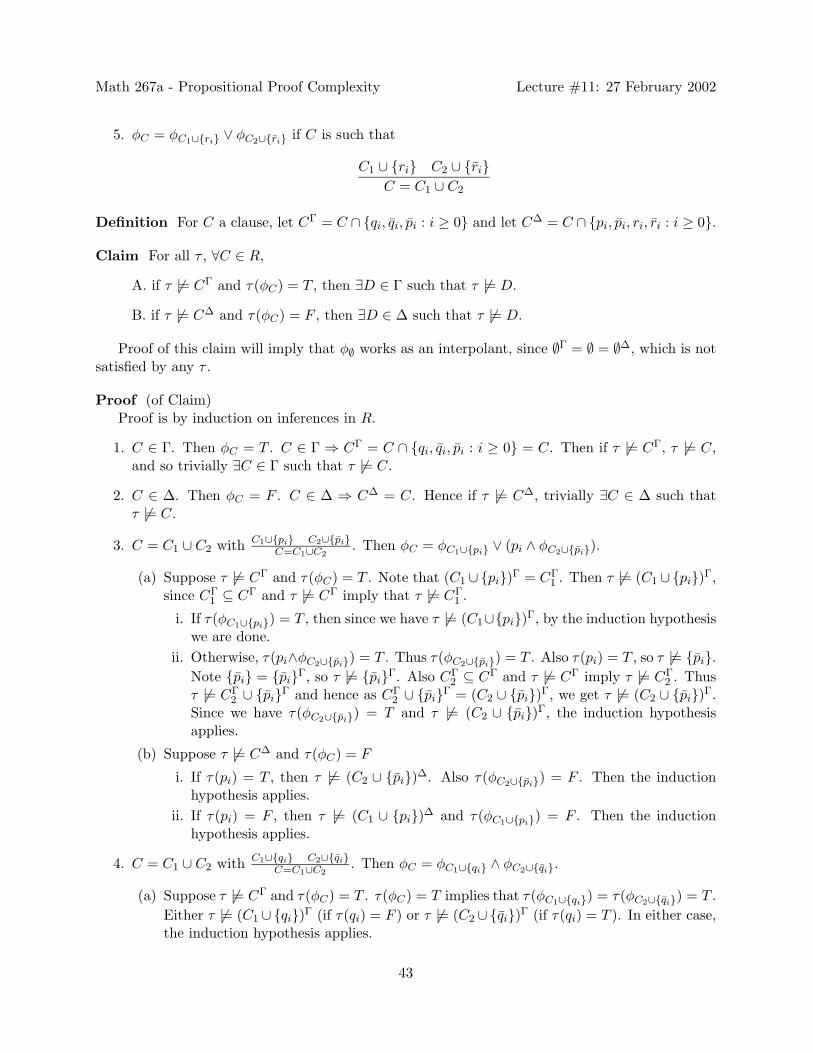
Math 267a - Propositional Proof Complexity Lecture #11: 27 February 2002
5. φC = φC1∪ri ∨ φC2∪ri if C is such that
C1 ∪ ri C2 ∪ riC = C1 ∪ C2
Definition For C a clause, let CΓ = C ∩ qi, qi, pi : i ≥ 0 and let C∆ = C ∩ pi, pi, ri, ri : i ≥ 0.
Claim For all τ , ∀C ∈ R,
A. if τ 6|= CΓ and τ(φC) = T , then ∃D ∈ Γ such that τ 6|= D.
B. if τ 6|= C∆ and τ(φC) = F , then ∃D ∈ ∆ such that τ 6|= D.
Proof of this claim will imply that φ∅ works as an interpolant, since ∅Γ = ∅ = ∅∆, which is notsatisfied by any τ .
Proof (of Claim)Proof is by induction on inferences in R.
1. C ∈ Γ. Then φC = T . C ∈ Γ ⇒ CΓ = C ∩ qi, qi, pi : i ≥ 0 = C. Then if τ 6|= CΓ, τ 6|= C,and so trivially ∃C ∈ Γ such that τ 6|= C.
2. C ∈ ∆. Then φC = F . C ∈ ∆ ⇒ C∆ = C. Hence if τ 6|= C∆, trivially ∃C ∈ ∆ such thatτ 6|= C.
3. C = C1 ∪ C2 with C1∪pi C2∪piC=C1∪C2
. Then φC = φC1∪pi ∨ (pi ∧ φC2∪pi).
(a) Suppose τ 6|= CΓ and τ(φC) = T . Note that (C1 ∪pi)Γ = CΓ1 . Then τ 6|= (C1 ∪pi)Γ,
since CΓ1 ⊆ CΓ and τ 6|= CΓ imply that τ 6|= CΓ
1 .
i. If τ(φC1∪pi) = T , then since we have τ 6|= (C1∪pi)Γ, by the induction hypothesiswe are done.
ii. Otherwise, τ(pi∧φC2∪pi) = T . Thus τ(φC2∪pi) = T . Also τ(pi) = T , so τ 6|= pi.Note pi = piΓ, so τ 6|= piΓ. Also CΓ
2 ⊆ CΓ and τ 6|= CΓ imply τ 6|= CΓ2 . Thus
τ 6|= CΓ2 ∪ piΓ and hence as CΓ
2 ∪ piΓ = (C2 ∪ pi)Γ, we get τ 6|= (C2 ∪ pi)Γ.Since we have τ(φC2∪pi) = T and τ 6|= (C2 ∪ pi)Γ, the induction hypothesisapplies.
(b) Suppose τ 6|= C∆ and τ(φC) = F
i. If τ(pi) = T , then τ 6|= (C2 ∪ pi)∆. Also τ(φC2∪pi) = F . Then the inductionhypothesis applies.
ii. If τ(pi) = F , then τ 6|= (C1 ∪ pi)∆ and τ(φC1∪pi) = F . Then the inductionhypothesis applies.
4. C = C1 ∪ C2 with C1∪qi C2∪qiC=C1∪C2
. Then φC = φC1∪qi ∧ φC2∪qi.
(a) Suppose τ 6|= CΓ and τ(φC) = T . τ(φC) = T implies that τ(φC1∪qi) = τ(φC2∪qi) = T .Either τ 6|= (C1 ∪qi)Γ (if τ(qi) = F ) or τ 6|= (C2 ∪qi)Γ (if τ(qi) = T ). In either case,the induction hypothesis applies.
43

Math 267a - Propositional Proof Complexity Lecture #11: 27 February 2002
(b) Suppose τ 6|= C∆ and τ(φC) = F . Note that (C1∪qi)∆ = C∆1 and (C2∪qi)∆ = C∆
2 .So τ 6|= (C1∪qi)∆ and τ 6|= (C2∪qi)∆. Also, since τ(φC) = F , either τ(φC1∪qi) = For τ(φC2∪qi) = F so in either case the induction hypothesis applies.
5. C = C1 ∪ C2 with C1∪ri C2∪riC=C1∪C2
. Then φC = φC1∪ri ∨ φC2∪ri.
(a) Suppose τ 6|= CΓ and τ(φC) = T . Note that (C1 ∪ ri)Γ = CΓ1 , and (C2 ∪ ri)Γ = CΓ
2 .Hence τ 6|= (C1∪ri)Γ and τ 6|= (C2∪ri)Γ. Also, τ(φC1∪ri) = T or τ(φC2∪ri) = T .Then the induction hypothesis applies to whichever one equals T .
(b) Suppose τ 6|= C∆ and τ(φC) = F . τ(φC) = F implies τ(φC1∪ri) = τ(φC2∪ri) = F .Either τ 6|= (C1 ∪ ri)∆ (if τ(ri) = F ) or τ 6|= (C2 ∪ ri)∆ (if τ(ri) = T ). In eithercase, the induction hypothesis applies.
Notice that φ is monotone in the pi’s.
23.3 Exponential Lower Bounds on Resolution Proofs for Clique and Coloring
Definition A k-coloring of a graph is an assignment of k colors to vertices such that no adjacentvertices have the same color.
Definition A k-clique in a graph is a subset consisting of k nodes such that for any pair of nodesin the subset there is an edge in the graph which joins them.
Theorem 35 A graph cannot have both a k + 1 clique and a k-coloring.
44

Math 267a - Propositional Proof Complexity Lecture #11: 27 February 2002
References
[1] S. R. Buss, Polynomial size proofs of the propositional pigeonhole principle, Journal of Sym-bolic Logic, 52 (1987), pp. 916–927.
[2] , Some remarks on lengths of propositional proofs, Archive for Mathematical Logic, 34(1995), pp. 377–394.
[3] S. A. Cook, Feasibly constructive proofs and the propositional calculus, in Proceedings of theSeventh Annual ACM Symposium on Theory of Computing, 1975, pp. 83–97.
[4] S. A. Cook and R. A. Reckhow, The relative efficiency of propositional proof systems,Journal of Symbolic Logic, 44 (1979), pp. 36–50.
[5] J. Krajıcek, Bounded Arithmetic, Propositional Calculus and Complexity Theory, CambridgeUniversity Press, Heidelberg, 1995.
[6] J. Krajıcek and P. Pudlak, Propositional proof systems, the consistency of first-order the-ories and the complexity of computations, Journal of Symbolic Logic, 54 (1989), pp. 1063–1079.
[7] R. J. Parikh, Some results on the lengths of proofs, Transactions of the American Mathemat-ical Society, 177 (1973), pp. 29–36.
[8] R. Statman, Complexity of derivations from quantifier-free Horn formulae, mechanical intro-duction of explicit definitions, and refinement of completeness theorems, in Logic Colloquium’76, R. Gandy and M. Hyland, eds., Amsterdam, 1977, North-Holland, pp. 505–517.
45