scilab textbook companion for electronic principles by a
TRANSCRIPT

Scilab Textbook Companion forElectronic Principles
by A. Malvino And D. J. Bates1
Created byNidhi Makhijani
B. TechComputer Engineering
IIT MandiCollege Teacher
NACross-Checked by
July 31, 2019
1Funded by a grant from the National Mission on Education through ICT,http://spoken-tutorial.org/NMEICT-Intro. This Textbook Companion and Scilabcodes written in it can be downloaded from the ”Textbook Companion Project”section at the website http://scilab.in

Book Description
Title: Electronic Principles
Author: A. Malvino And D. J. Bates
Publisher: Tata McGraw - Hill, New Delhi
Edition: 7
Year: 2007
ISBN: 978-0-07-063424-4
1

Scilab numbering policy used in this document and the relation to theabove book.
Exa Example (Solved example)
Eqn Equation (Particular equation of the above book)
AP Appendix to Example(Scilab Code that is an Appednix to a particularExample of the above book)
For example, Exa 3.51 means solved example 3.51 of this book. Sec 2.3 meansa scilab code whose theory is explained in Section 2.3 of the book.
2
Contents
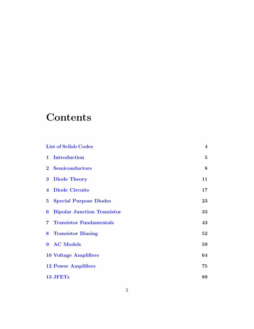
List of Scilab Codes 4
1 Introduction 5
2 Semiconductors 8
3 Diode Theory 11
4 Diode Circuits 17
5 Special Purpose Diodes 23
6 Bipolar Junction Transistor 33
7 Transistor Fundamentals 43
8 Transistor Biasing 52
9 AC Models 59
10 Voltage Amplifiers 64
12 Power Amplifiers 75
13 JFETs 89
3

14 MOSFETs 101
15 Thyristors 111
16 Frequency Effects 116
17 Differential Amplifiers 124
18 Operational Amplifiers 135
19 Negative Feedback 145
20 Linear Op Amp Circuits 154
21 Active Filters 162
22 Non Linear Op Amp Circuits 174
23 Oscillators 181
24 Regulated Power Supplies 190
4
List of Scilab Codes
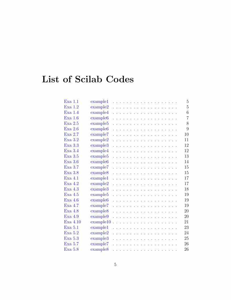
Exa 1.1 example1 . . . . . . . . . . . . . . . . . . . 5Exa 1.2 example2 . . . . . . . . . . . . . . . . . . . 5Exa 1.4 example4 . . . . . . . . . . . . . . . . . . . 6Exa 1.6 example6 . . . . . . . . . . . . . . . . . . . 7Exa 2.5 example5 . . . . . . . . . . . . . . . . . . . 8Exa 2.6 example6 . . . . . . . . . . . . . . . . . . . 9Exa 2.7 example7 . . . . . . . . . . . . . . . . . . . 10Exa 3.2 example2 . . . . . . . . . . . . . . . . . . . 11Exa 3.3 example3 . . . . . . . . . . . . . . . . . . . 12Exa 3.4 example4 . . . . . . . . . . . . . . . . . . . 12Exa 3.5 example5 . . . . . . . . . . . . . . . . . . . 13Exa 3.6 example6 . . . . . . . . . . . . . . . . . . . 14Exa 3.7 example7 . . . . . . . . . . . . . . . . . . . 15Exa 3.8 example8 . . . . . . . . . . . . . . . . . . . 15Exa 4.1 example1 . . . . . . . . . . . . . . . . . . . 17Exa 4.2 example2 . . . . . . . . . . . . . . . . . . . 17Exa 4.3 example3 . . . . . . . . . . . . . . . . . . . 18Exa 4.5 example5 . . . . . . . . . . . . . . . . . . . 19Exa 4.6 example6 . . . . . . . . . . . . . . . . . . . 19Exa 4.7 example7 . . . . . . . . . . . . . . . . . . . 19Exa 4.8 example8 . . . . . . . . . . . . . . . . . . . 20Exa 4.9 example9 . . . . . . . . . . . . . . . . . . . 20Exa 4.10 example10 . . . . . . . . . . . . . . . . . . . 21Exa 5.1 example1 . . . . . . . . . . . . . . . . . . . 23Exa 5.2 example2 . . . . . . . . . . . . . . . . . . . 24Exa 5.3 example3 . . . . . . . . . . . . . . . . . . . 25Exa 5.7 example7 . . . . . . . . . . . . . . . . . . . 26Exa 5.8 example8 . . . . . . . . . . . . . . . . . . . 26
5

Exa 5.10 example10 . . . . . . . . . . . . . . . . . . . 27Exa 5.11 example11 . . . . . . . . . . . . . . . . . . . 28Exa 5.12 example12 . . . . . . . . . . . . . . . . . . . 29Exa 5.13 example13 . . . . . . . . . . . . . . . . . . . 29Exa 5.14 example14 . . . . . . . . . . . . . . . . . . . 30Exa 5.15 example15 . . . . . . . . . . . . . . . . . . . 31Exa 6.1 example1 . . . . . . . . . . . . . . . . . . . 33Exa 6.2 example2 . . . . . . . . . . . . . . . . . . . 34Exa 6.3 example3 . . . . . . . . . . . . . . . . . . . 34Exa 6.4 example4 . . . . . . . . . . . . . . . . . . . 35Exa 6.5 example5 . . . . . . . . . . . . . . . . . . . 36Exa 6.6 example6 . . . . . . . . . . . . . . . . . . . 37Exa 6.7 example7 . . . . . . . . . . . . . . . . . . . 38Exa 6.8 example8 . . . . . . . . . . . . . . . . . . . 39Exa 6.9 example9 . . . . . . . . . . . . . . . . . . . 40Exa 6.11 example11 . . . . . . . . . . . . . . . . . . . 41Exa 6.12 example12 . . . . . . . . . . . . . . . . . . . 41Exa 7.1 example1 . . . . . . . . . . . . . . . . . . . 43Exa 7.2 example2 . . . . . . . . . . . . . . . . . . . 44Exa 7.3 example3 . . . . . . . . . . . . . . . . . . . 44Exa 7.4 example4 . . . . . . . . . . . . . . . . . . . 45Exa 7.5 example5 . . . . . . . . . . . . . . . . . . . 46Exa 7.6 example6 . . . . . . . . . . . . . . . . . . . 47Exa 7.7 example7 . . . . . . . . . . . . . . . . . . . 48Exa 7.8 example8 . . . . . . . . . . . . . . . . . . . 49Exa 7.9 example9 . . . . . . . . . . . . . . . . . . . 50Exa 8.1 example1 . . . . . . . . . . . . . . . . . . . 52Exa 8.3 example3 . . . . . . . . . . . . . . . . . . . 53Exa 8.4 example4 . . . . . . . . . . . . . . . . . . . 54Exa 8.5 example5 . . . . . . . . . . . . . . . . . . . 55Exa 8.6 example6 . . . . . . . . . . . . . . . . . . . 56Exa 8.7 example7 . . . . . . . . . . . . . . . . . . . 57Exa 9.1 example1 . . . . . . . . . . . . . . . . . . . 59Exa 9.2 example2 . . . . . . . . . . . . . . . . . . . 60Exa 9.3 example3 . . . . . . . . . . . . . . . . . . . 60Exa 9.4 example4 . . . . . . . . . . . . . . . . . . . 61Exa 9.5 example5 . . . . . . . . . . . . . . . . . . . 62Exa 9.6 example6 . . . . . . . . . . . . . . . . . . . 63
6
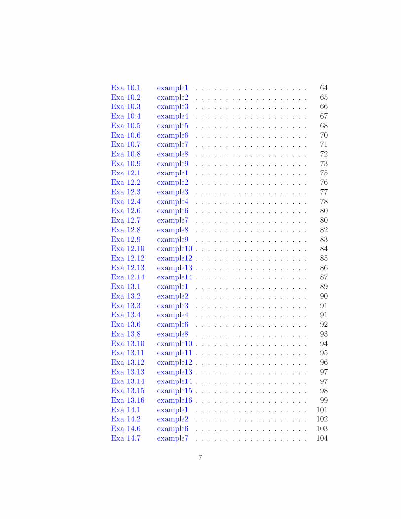
Exa 10.1 example1 . . . . . . . . . . . . . . . . . . . 64Exa 10.2 example2 . . . . . . . . . . . . . . . . . . . 65Exa 10.3 example3 . . . . . . . . . . . . . . . . . . . 66Exa 10.4 example4 . . . . . . . . . . . . . . . . . . . 67Exa 10.5 example5 . . . . . . . . . . . . . . . . . . . 68Exa 10.6 example6 . . . . . . . . . . . . . . . . . . . 70Exa 10.7 example7 . . . . . . . . . . . . . . . . . . . 71Exa 10.8 example8 . . . . . . . . . . . . . . . . . . . 72Exa 10.9 example9 . . . . . . . . . . . . . . . . . . . 73Exa 12.1 example1 . . . . . . . . . . . . . . . . . . . 75Exa 12.2 example2 . . . . . . . . . . . . . . . . . . . 76Exa 12.3 example3 . . . . . . . . . . . . . . . . . . . 77Exa 12.4 example4 . . . . . . . . . . . . . . . . . . . 78Exa 12.6 example6 . . . . . . . . . . . . . . . . . . . 80Exa 12.7 example7 . . . . . . . . . . . . . . . . . . . 80Exa 12.8 example8 . . . . . . . . . . . . . . . . . . . 82Exa 12.9 example9 . . . . . . . . . . . . . . . . . . . 83Exa 12.10 example10 . . . . . . . . . . . . . . . . . . . 84Exa 12.12 example12 . . . . . . . . . . . . . . . . . . . 85Exa 12.13 example13 . . . . . . . . . . . . . . . . . . . 86Exa 12.14 example14 . . . . . . . . . . . . . . . . . . . 87Exa 13.1 example1 . . . . . . . . . . . . . . . . . . . 89Exa 13.2 example2 . . . . . . . . . . . . . . . . . . . 90Exa 13.3 example3 . . . . . . . . . . . . . . . . . . . 91Exa 13.4 example4 . . . . . . . . . . . . . . . . . . . 91Exa 13.6 example6 . . . . . . . . . . . . . . . . . . . 92Exa 13.8 example8 . . . . . . . . . . . . . . . . . . . 93Exa 13.10 example10 . . . . . . . . . . . . . . . . . . . 94Exa 13.11 example11 . . . . . . . . . . . . . . . . . . . 95Exa 13.12 example12 . . . . . . . . . . . . . . . . . . . 96Exa 13.13 example13 . . . . . . . . . . . . . . . . . . . 97Exa 13.14 example14 . . . . . . . . . . . . . . . . . . . 97Exa 13.15 example15 . . . . . . . . . . . . . . . . . . . 98Exa 13.16 example16 . . . . . . . . . . . . . . . . . . . 99Exa 14.1 example1 . . . . . . . . . . . . . . . . . . . 101Exa 14.2 example2 . . . . . . . . . . . . . . . . . . . 102Exa 14.6 example6 . . . . . . . . . . . . . . . . . . . 103Exa 14.7 example7 . . . . . . . . . . . . . . . . . . . 104
7
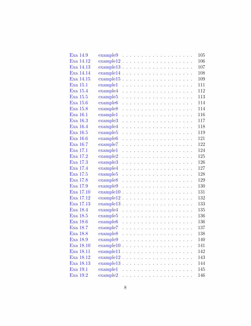
Exa 14.9 example9 . . . . . . . . . . . . . . . . . . . 105Exa 14.12 example12 . . . . . . . . . . . . . . . . . . . 106Exa 14.13 example13 . . . . . . . . . . . . . . . . . . . 107Exa 14.14 example14 . . . . . . . . . . . . . . . . . . . 108Exa 14.15 example15 . . . . . . . . . . . . . . . . . . . 109Exa 15.1 example1 . . . . . . . . . . . . . . . . . . . 111Exa 15.4 example4 . . . . . . . . . . . . . . . . . . . 112Exa 15.5 example5 . . . . . . . . . . . . . . . . . . . 113Exa 15.6 example6 . . . . . . . . . . . . . . . . . . . 114Exa 15.8 example8 . . . . . . . . . . . . . . . . . . . 114Exa 16.1 example1 . . . . . . . . . . . . . . . . . . . 116Exa 16.3 example3 . . . . . . . . . . . . . . . . . . . 117Exa 16.4 example4 . . . . . . . . . . . . . . . . . . . 118Exa 16.5 example5 . . . . . . . . . . . . . . . . . . . 119Exa 16.6 example6 . . . . . . . . . . . . . . . . . . . 121Exa 16.7 example7 . . . . . . . . . . . . . . . . . . . 122Exa 17.1 example1 . . . . . . . . . . . . . . . . . . . 124Exa 17.2 example2 . . . . . . . . . . . . . . . . . . . 125Exa 17.3 example3 . . . . . . . . . . . . . . . . . . . 126Exa 17.4 example4 . . . . . . . . . . . . . . . . . . . 127Exa 17.5 example5 . . . . . . . . . . . . . . . . . . . 128Exa 17.8 example8 . . . . . . . . . . . . . . . . . . . 129Exa 17.9 example9 . . . . . . . . . . . . . . . . . . . 130Exa 17.10 example10 . . . . . . . . . . . . . . . . . . . 131Exa 17.12 example12 . . . . . . . . . . . . . . . . . . . 132Exa 17.13 example13 . . . . . . . . . . . . . . . . . . . 133Exa 18.4 example4 . . . . . . . . . . . . . . . . . . . 135Exa 18.5 example5 . . . . . . . . . . . . . . . . . . . 136Exa 18.6 example6 . . . . . . . . . . . . . . . . . . . 136Exa 18.7 example7 . . . . . . . . . . . . . . . . . . . 137Exa 18.8 example8 . . . . . . . . . . . . . . . . . . . 138Exa 18.9 example9 . . . . . . . . . . . . . . . . . . . 140Exa 18.10 example10 . . . . . . . . . . . . . . . . . . . 141Exa 18.11 example11 . . . . . . . . . . . . . . . . . . . 142Exa 18.12 example12 . . . . . . . . . . . . . . . . . . . 143Exa 18.13 example13 . . . . . . . . . . . . . . . . . . . 144Exa 19.1 example1 . . . . . . . . . . . . . . . . . . . 145Exa 19.2 example2 . . . . . . . . . . . . . . . . . . . 146
8

Exa 19.3 example3 . . . . . . . . . . . . . . . . . . . 147Exa 19.4 example4 . . . . . . . . . . . . . . . . . . . 148Exa 19.6 example6 . . . . . . . . . . . . . . . . . . . 149Exa 19.9 example9 . . . . . . . . . . . . . . . . . . . 150Exa 19.10 example10 . . . . . . . . . . . . . . . . . . . 150Exa 19.11 example11 . . . . . . . . . . . . . . . . . . . 151Exa 19.12 example12 . . . . . . . . . . . . . . . . . . . 152Exa 19.13 example13 . . . . . . . . . . . . . . . . . . . 153Exa 20.2 example2 . . . . . . . . . . . . . . . . . . . 154Exa 20.3 example3 . . . . . . . . . . . . . . . . . . . 155Exa 20.5 example5 . . . . . . . . . . . . . . . . . . . 156Exa 20.6 example6 . . . . . . . . . . . . . . . . . . . 157Exa 20.7 example7 . . . . . . . . . . . . . . . . . . . 158Exa 20.8 example8 . . . . . . . . . . . . . . . . . . . 159Exa 20.9 example9 . . . . . . . . . . . . . . . . . . . 160Exa 20.10 example10 . . . . . . . . . . . . . . . . . . . 160Exa 21.1 example1 . . . . . . . . . . . . . . . . . . . 162Exa 21.2 example2 . . . . . . . . . . . . . . . . . . . 163Exa 21.3 example3 . . . . . . . . . . . . . . . . . . . 164Exa 21.4 example4 . . . . . . . . . . . . . . . . . . . 165Exa 21.5 example5 . . . . . . . . . . . . . . . . . . . 166Exa 21.6 example6 . . . . . . . . . . . . . . . . . . . 167Exa 21.7 example7 . . . . . . . . . . . . . . . . . . . 168Exa 21.9 example9 . . . . . . . . . . . . . . . . . . . 169Exa 21.10 example10 . . . . . . . . . . . . . . . . . . . 170Exa 21.12 example12 . . . . . . . . . . . . . . . . . . . 171Exa 21.13 example13 . . . . . . . . . . . . . . . . . . . 172Exa 22.4 example4 . . . . . . . . . . . . . . . . . . . 174Exa 22.5 example5 . . . . . . . . . . . . . . . . . . . 175Exa 22.6 example6 . . . . . . . . . . . . . . . . . . . 176Exa 22.7 example7 . . . . . . . . . . . . . . . . . . . 177Exa 22.8 example8 . . . . . . . . . . . . . . . . . . . 178Exa 22.10 example10 . . . . . . . . . . . . . . . . . . . 178Exa 22.12 example12 . . . . . . . . . . . . . . . . . . . 179Exa 23.1 example1 . . . . . . . . . . . . . . . . . . . 181Exa 23.2 example2 . . . . . . . . . . . . . . . . . . . 182Exa 23.4 example4 . . . . . . . . . . . . . . . . . . . 183Exa 23.5 example5 . . . . . . . . . . . . . . . . . . . 183
9

Exa 23.6 example6 . . . . . . . . . . . . . . . . . . . 184Exa 23.7 example7 . . . . . . . . . . . . . . . . . . . 185Exa 23.8 example8 . . . . . . . . . . . . . . . . . . . 186Exa 23.10 example10 . . . . . . . . . . . . . . . . . . . 187Exa 23.12 example12 . . . . . . . . . . . . . . . . . . . 188Exa 24.1 example1 . . . . . . . . . . . . . . . . . . . 190Exa 24.2 example2 . . . . . . . . . . . . . . . . . . . 191Exa 24.3 example3 . . . . . . . . . . . . . . . . . . . 192Exa 24.4 example4 . . . . . . . . . . . . . . . . . . . 193Exa 24.6 example6 . . . . . . . . . . . . . . . . . . . 194Exa 24.7 example7 . . . . . . . . . . . . . . . . . . . 195Exa 24.8 example8 . . . . . . . . . . . . . . . . . . . 196Exa 24.10 example10 . . . . . . . . . . . . . . . . . . . 197Exa 24.13 example13 . . . . . . . . . . . . . . . . . . . 198Exa 24.15 example15 . . . . . . . . . . . . . . . . . . . 199Exa 24.16 example16 . . . . . . . . . . . . . . . . . . . 199
10

Chapter 1
Introduction
Scilab code Exa 1.1 example1
1
2 // Example 1−1 , page 93
4 clear;clc; close;
5
6 // Given data7 R(1) =50; // s ou r c e r e s i s t a n c e o f ac v o l t a g e i n ohms8
9 // Ca l c u l a t i o n s10 R(2)=R(1) *100; // minimum load r e s i s t a n c e11 disp(”ohms”, R(2),”Load r e s i s t a n c e =”)
Scilab code Exa 1.2 example2
1
2 // Example 1−2 , page 123
11

4 clear;clc; close;
5
6 // Given data7 i=2; // c u r r e n t source , i n m i l l i amperes8 R=10*10^6; // i n t e r n a l s o u r c e r e s i s t a n c e , i n ohms9
10 // Ca l c u l a t i o n s11 Rlmin =0; // minimum load r e s i s t a n c e i n ohms12 Rlmax =0.01*R; // maximum load r e s i s t a n c e13 disp(”ohms”, Rlmin ,”Minimum Load r e s i s t a n c e =”)14 disp(”ohms”, Rlmax ,”Maximum Load r e s i s t a n c e =”)
Scilab code Exa 1.4 example4
1 // f i n d th ev en i n v o l t a g e and r e s i s t a n c e2 // E l e c t r o n i c P r i n c i p l e s3 // By Albe r t Malvino , David Bates4 // Seventh Ed i t i o n5 // The McGraw−H i l l Companies6 // Example 1−4 , page 147
8 clear;clc; close;
9
10 // Given data11 Vs=72; // s ou r c e v o l t a g e i n v o l t s12
13 // Ca l c u l a t i o n s14 // open l oad r e s i s t o r to g e t th ev en i n v o l t a g e15 Vth =24; // i n v o l t s as 8 mA f l ow s through 6Kohms in
s e r i e s with 3Kohms , no c u r r e n t through 4Kohms16 // r educe s ou r c e to z e r o to g e t th ev en i n r e s i s t a n c e17 Rth =4+((3*6) /(3+6));// i n Kohms18
12
19 disp(” Vo l t s ”, Vth ,”Thevenin Vo l tage =”)20 disp(”ohms”,Rth ,”Thevenin Re s i s t a n c e =”)21
22 // Re su l t23 // Thevenin v o l t a g e i s 24 v o l t s24 // Thevenin r e s i s t a n c e i s 6 Kohms
Scilab code Exa 1.6 example6
1
2
3
4
5
6 // Given data7 Vth =10; // Thevenin v o l t a g e i n v o l t s8 Rth =2000; // Thevenin r e s i s t a n c e i n ohms9
10 // Ca l c u l a t i o n s11 In=Vth/Rth;// Norton c u r r e n t i n amperes12 disp(”Amperes ”,In ,”Norton Current=”)
13

Chapter 2
Semiconductors
Scilab code Exa 2.5 example5
1
2
3
4 // Given data5 V(1) =0.7; // b a r r i e r p o t e n t i a l i n v o l t s at 25 deg r e e
c e l c i u s6 T(1) =25; // t empera tu re i n d eg r e e c e l c i u s at which
v b a r r i e r p o t e n t i a l i s known7 T(2) =100; T(3)=0; // t empera tu r e i n d eg r e e c e l c i u s
at which b a r r i e r p o t e n t i a l has to be found8
9 // C a l c u l a t i o n s10 dT(2)=T(2)-T(1);// d i f f e r e n c e i n t empera tu re11 dT(3)=T(3)-T(1);// d i f f e r e n c e i n t empera tu re12 dV(3) =( -0.002)*dT(3);// b a r r i e r p o t e n t i a l f o r
s i l i c o n d e c r e a s e s by 0 . 0 0 2 v o l t s f o r each deg r e ec e l c i u s r i s e
13 dV(2) =( -0.002)*dT(2) // b a r r i e r p o t e n t i a l f o r s i l i c o nd e c r e a s e s by 0 . 0 02 v o l t s f o r each deg r e e c e l c i u sr i s e
14 V(2)=V(1)+dV(2);// to f i n d b a r r i e r p o t e n t i a l a t T( 2 )
14

15 V(3)=V(1)+dV(3);// to f i n d b a r r i e r p o t e n t i a l a t T( 3 )16 disp(” Vo l t s ”,V(2),” Ba r r i e r P o t e n t i a l a t 100 Degree
c e l c i u s =”)17 disp(” Vo l t s ”,V(3),” Ba r r i e r P o t e n t i a l a t 0 Degree
c e l c i u s =”)18
19 // Re su l t20 // b a r r i e r p o t e n t i a l a t 100 deg r e e c e l c i u s i s 0 . 5 5
v o l t s21 // b a r r i e r p o t e n t i a l a t 0 d eg r e e c e l c i u s i s 0 . 7 5
v o l t s
Scilab code Exa 2.6 example6
1
2 // Example 2−6 , page 513
4 clear;clc; close;
5
6 // Given data7 I(1)=5; // s a t u r a t i o n c u r r e n t at g i v en t empera tu r e i n
nano amperes8 T(1) =25; // t empera tu r e i n d eg r e e c e l c i u s at which
s a t u r a t i o n c u r r e n t i s known9 T(2) =100; // t empera tu re i n d eg r e e c e l c i u s at which
s a t u r a t i o n c u r r e n t i s to be found10
11 // Ca l c u l a t i o n s12 I(2) =(2^7)*I(1);// 7 doub l i n g s between 25 and 95
deg r e e c e l c i u s13 I(3) =((1.07) ^5)*I(2); // a d d i t i o n a l 5 d eg r e e between
95 and 100 deg r e e c e l c i u s14 disp(”Amperes ”,I(3),” S a t u r a t i o n Current =”)
15

15
16 // Re su l t17 // s a t u r a t i o n c u r r e n t at 100 deg r e e c e l c i u s i s 898
nano amperes .
Scilab code Exa 2.7 example7
1
2 // Example 2−7 , page 523
4 clear;clc; close;
5
6 // Given data7 I(1) =2*10^ -9; // s u r f a c e l e a k a g e c u r r e n t i n amperes
at g i v en r e v e r s e v o l t a g e8 V(1) =25; // r e v e r s e v o l t a g e i n v o l t s at which s u r f a c e
l e a k a g e i s known9 V(2) =35; // r e v e r s e v o l t a g e i n v o l t s at which s u r f a c e
l e a k a g e c u r r e n t i s to be found10
11 // Ca l c u l a t i o n s12 I(2)=V(2)*I(1)/V(1);// s u r f a c e l e a k a g e c u r r e n t i s
d i r e c t l y p r o p o r t i o n a l to r e v e r s e v o l t a g e13 disp(”Amperes ”,I(2),” Su r f a c e l e a k a g e Current =”)14
15 // r e s u l t16 // s u r f a c e l e a k a g e c u r r e n t i s 2 . 8 nano amperes .
16

Chapter 3
Diode Theory
Scilab code Exa 3.2 example2
1
2 // Example 3−2 , page 633
4 clear;clc; close;
5
6 // Given data7 v=1.2; // d i ode v o l t a g e i n v o l t s8 i=1.75; // d i ode c u r r e n t i n amperes9 P(1)=5; // power r a t i n g i n watt s
10
11 // Ca l c u l a t i o n s12 P(2)=v*i; // power d i s s i p a t i o n13 disp(”Watts ”,P(2),”Power d i s s i p a t i o n ”)14
15 // Re su l t16 // As power d i s s i p a t i o n i s l owe r than power r a t i n g
the d i ode w i l l not g e t d e s t r o y ed .
17

Scilab code Exa 3.3 example3
1 // to f i n d l oad v o l t a g e and l oad cu r r e n t u s i n g i d e a ld i ode
2
3 // Example 3−3 , page 654
5 clear;clc; close;
6
7 // Given data8 // d i ode i s f o rward b ia s ed , e q u i v a l e n t to a c l o s e d
sw i t ch .9
10 // Ca l c u l a t i o n s11 V=10; // l oad v o l t a g e i n v o l t s12 R=1000; // l oad r e s i s t a n c e i n ohms13 I=V/R;// a l l the s ou r c e v o l t a g e appea r s a c r o s s the
l oad r e s i s t o r14 disp(”Amperes ”,I,”Load Current=”)15 disp(” Vo l t s ”,V,”Load Vo l tage=”)
Scilab code Exa 3.4 example4
1
2 // Example 3−4 , page 65 ‘3
4 clear;clc; close;
5
18

6 // Given data7 // r e f e r to the diagram , t h e v e n i z e the c i r c u i t to
the l e f t o f the d i ode .8 // l o o k i n g at the d i ode back toward the source , we
s e e a v o l t a g e d i v i d e r with 6 k i l l o −ohms and 3k i l l o −ohms .
9 R=2000; // th ev en i n r e s i s t a n c e i n ohms10 V=12; // th ev en i n v o l t a g e i n v o l t s11
12 // Ca l c u l a t i o n s13 disp(”Using Thevenin Thm”)14 // we have a s e r i e s c i r c u i t and the d i ode i s f o rward
b i a s e d .15 // v i s u a l i z e the d i ode as a c l o s e d sw i t ch16 I=V/3000; // l oad c u r r e n t i n amperes17 V(1)=I*1000; // l oad v o l t a g e18 disp(”Amperes ”,I,”Load Current=”)19 disp(” Vo l t s ”,V(1),”Load Vo l tage=”)
Scilab code Exa 3.5 example5
1
2 // Example 3−5 , page 67 ‘3
4 clear;clc; close;
5
6 // Given data7 // the d i ode i s f o rward b ia s ed , e q u i v a l e n t to a
ba t t e r y o f 0 . 7 v o l t s8 V=10; // v o l t a g e o f b a t t e r y i n v o l t s9 Vd=0.7; // d i ode drop i n v o l t s10
11 // Ca l c u l a t i o n s
19

12 Vl=V-Vd;// l oad v o l t a g e i n v o l t s13 R=1000; // l oad r e s i s t a n c e i n ohms14 Il=Vl/R;// l oad c u r r e n t i n amperes15 Pd=Il*Vd;// d i ode power i n watt s16 disp(”Amperes ”,Il ,”Load Current=”)17 disp(” Vo l t s ”,Vl ,”Load Vo l tage=”)18 disp(”Watts ”,Pd ,”Diode power=”)
Scilab code Exa 3.6 example6
1
2 // Example 3−6 , page 67 ‘3
4 clear;clc; close;
5
6 // Given data7 // t h e v e n i z e the c i r c u i t to the l e f t o f the d i ode .8 // l o o k i n g at the d i ode back toward the source , we
s e e a v o l t a g e d i v i d e r with 6 k i l l o −ohms and 3k i l l o −ohms .
9 R=2000; // th ev en i n r e s i s t a n c e i n ohms10 V(1) =12; // th ev en i n v o l t a g e i n v o l t s11
12 // Ca l c u l a t i o n s13 disp(”Using Thevenin Thm”)14 V(2) =0.7; // d i ode v o l t a g e i n v o l t s15 I=(V(1)-V(2))/3000 // l oad c u r r e n t i n amperes16 P=V(2)*I // d i ode power i n watt s17 V=I*1000 // l oad v o l t a g e i n v o l t s18 disp(”Amperes ”,I,”Load Current=”)19 disp(” Vo l t s ”,V,”Load Vo l tage=”)20 disp(”Watts ”,P,”Diode power=”)
20

Scilab code Exa 3.7 example7
1
2 // Example 3−7 , page 683
4 clear;clc; close;
5
6 // Given data7 Vd=0.7; // d i ode drop in v o l t s8 V=10; // s ou r c e v o l t a g e9 R=1000; // r e s i s t a n c e i n ohms10
11 // Ca l c u l a t i o n s12 Vl=V-Vd;// l oad v o l t a g e i n v o l t s13 I=Vl/R;// l oad c u r r e n t i n amperes14 P=(V-Vl)*I;// d i ode power i n watt s15 disp(”Amperes ”,I,”Load Current=”)16 disp(” Vo l t s ”,Vl ,”Load Vo l tage=”)17 disp(”Watts ”,P,”Diode power=”)
Scilab code Exa 3.8 example8
1
2 // Example 3−8 , page 69 ‘3
4 clear;clc; close;
5
6 // Given data
21

7 Rl=10; // l oad r e s i s t a n c e i n ohms8 Rb =0.23; // bulk r e s i s t a n c e i n ohms9 // d i ode drop =0.7 v o l t s10
11 // Ca l c u l a t i o n s12 Rt=Rl+Rb;// t o t a l r e s i s t a n c e i n ohms13 Vt=10 -0.7; // v o l t a g e o f ba t t e ry−d iode drop14 I=Vt/Rt;// l oad c u r r e n t15 Vl=I*10; // l oad v o l t a g e16 Vd=10-Vl;// s ou r c e vo l t a g e−l o ad v o l t a g e17 P=Vd*I;
18 disp(”Amperes ”,I,”Load Current=”)19 disp(” Vo l t s ”,Vl ,”Load Vo l tage=”)20 disp(”Watts ”,P,”Diode power=”)
22

Chapter 4
Diode Circuits
Scilab code Exa 4.1 example1
1 //Theory Example
Scilab code Exa 4.2 example2
1
2 // Example 4−2 , page 953
4 clear;clc; close;
5
6 // Given data7 // r e f e r to the diagram8 // tu rn s r a t i o 5 : 19 V1=120; // pr imary v o l t a g e i n v o l t s10
11 // Ca l c u l a t i o n s12
13 V2=V1/5; // s e conda ry v o l t a g e i n v o l t s
23

14 Vpin=V2 /0.707; // peak s e conda ry v o l t a g e i n v o l t s15 // with i d e a l d i ode16 Vpout=Vpin;
17 Vdc=Vpout/%pi;
18 disp(” Vo l t s ”,Vpout ,”Peak v o l t a g e =”)19 disp(” Vo l t s ”,Vdc ,”dc l oad v o l t a g e=”)20 // with second approx imat i on21
22 Vpout=Vpin -0.7; // peak l oad v o l t a g e i n v o l t s23 Vdc=Vpout/%pi;
24 disp(” Vo l t s ”,Vpout ,”Peak v o l t a g e =”)25 disp(” Vo l t s ”,Vdc ,”dc l oad v o l t a g e=”)
Scilab code Exa 4.3 example3
1
2 // Example 4−3 , page 973
4 clear;clc; close;
5
6 // Given data7 Vrms =120; // i n v o l t s8 // 10 : 1 s t e p down t r a n s f o rme r9
10 // Ca l c u l a t i o n s11
12 Vp1=Vrms /0.707; // peak pr imary v o l t a g e i n v o l t s13 Vp2=Vp1 /10; // peak s e conda ry v o l t a g e i n v o l t s14 // the f u l l wave r e c t i f i e r a c t s l i k e 2 back−to−back
ha l f−wave r e c t i f i e r s . b e caus e o f the c e n t e r tap ,the input v o l t a g e to each ha l f−wave r e c t i f i e r i son ly h a l f the s e condary v o l t a g e
15 Vpin =0.5* Vp2;
24
16 disp(” Vo l t s ”,Vpin ,”Peak input v o l t a g e =”)17
18 Vpout=Vpin;// i d e a l l y19 disp(” Vo l t s ”,Vpout ,”Peak v o l t a g e =”)20
21 Vpout=Vpin -0.7; // u s i n g second approx imat ion22 disp(” Vo l t s ”,Vpout ,”Peak v o l t a g e =”)
Scilab code Exa 4.5 example5
1 //Theory Example
Scilab code Exa 4.6 example6
1 //Theory Example
Scilab code Exa 4.7 example7
1 //Theory Example
25
Scilab code Exa 4.8 example8
1 // c a l c u l a t i n g o f dc l oad v o l t a g e and r i p p l e2 // E l e c t r o n i c P r i n c i p l e s3 // By Albe r t Malvino , David Bates4 // Seventh Ed i t i o n5 // The McGraw−H i l l Companies6 // Example 4−8 , page 1107
8 clear;clc; close;
9
10 // Given data11 V1=120; // rms input v o l t a g e i n v o l t s12 Rl =5000; // dc l oad r e s i s t a n c e i n ohms13 f=60; // f r e qu en cy in h e r t z14 C=100*10^ -6 // c a p a c i t a n c e i n f a r a d s15 // 5 : 1 s t e p down t r a n s f o rme r16
17 // Ca l c u l a t i o n s18 V2=V1/5; // rms s e conda ry v o l t a g e i n v o l t s19 Vp=V2 /0.707; // peak s e conda ry v o l t a g e20 Vl=Vp;// i d e a l d i ode and sma l l r i p p l e21 Il=Vl/Rl;// dc l oad c u r r e n t i n amperes22 Vr=Il/(2*f*C);// r i p p l e i n vpp , b r i d g e r e c t i f i e r23 disp(” Vo l t s ”,Vl ,”dc l oad v o l t a g e =”)24 disp(” Vo l t s ”,Vr ,” r i p l e =”)25
26 // Re su l t27 // dc l oad v o l t a g e i s 34 v o l t s28 // r i p p l e i s 0 . 5 7 Vpp
Scilab code Exa 4.9 example9
26

1 // c a l c u l a t i n g o f dc l oad v o l t a g e and r i p p l e2 // E l e c t r o n i c P r i n c i p l e s3 // By Albe r t Malvino , David Bates4 // Seventh Ed i t i o n5 // The McGraw−H i l l Companies6 // Example 4−9 , page 1117
8 clear;clc; close;
9
10 // Given data11 V1=120; // rms input v o l t a g e i n v o l t s12 Rl=500; // dc l oad r e s i s t a n c e i n ohms13 f=60; // f r e qu en cy in h e r t z14 C=4700*10^ -6 // c a p a c i t a n c e i n f a r a d s15 // 15 : 1 s t e p down t r a n s f o rme r16
17 // Ca l c u l a t i o n s18 V2=V1/15; // rms s e conda ry v o l t a g e i n v o l t s19 Vp=V2 /0.707; // peak s e conda ry v o l t a g e20 Vl=Vp -1.4; // u s i n g second approx imat ion21 Il=Vl/Rl;// dc l oad c u r r e n t i n amperes22 Vr=Il/(2*f*C);// r i p p l e i n vpp , b r i d g e r e c t i f i e r23 disp(” Vo l t s ”,Vl ,”dc l oad v o l t a g e =”)24 disp(” Vo l t s ”,Vr ,” r i p l e =”)25
26 // Re su l t27 // dc l oad v o l t a g e i s 9 . 9 v o l t s28 // r i p p l e i s 35 mVpp
Scilab code Exa 4.10 example10
1
2 // Example 4−10 , page 114
27

3
4 clear;clc; close;
5
6 // Given data7 V1=120; // rms input v o l t a g e i n v o l t s8 // tu rn s r a t i o 8 : 19
10 // Ca l c u l a t i o n s11 V2=V1/8; // rms s e conda ry v o l t a g e i n v o l t s12 Vp=V2 /0.707; // peak s e conda ry v o l t a g e13 PIV=Vp;// peak i n v e r s e v o l t a g e14 disp(PIV)
15 disp(” Vo l t s ”,PIV ,”Peak i n v e r s e v o l t a g e =”)16
17 // Re su l t18 // peak i n v e r s e v o l t a g e i s 2 1 . 2 v o l t s
28

Chapter 5
Special Purpose Diodes
Scilab code Exa 5.1 example1
1 // f i n d minimum and maximum zene r c u r r e n t s2 // E l e c t r o n i c P r i n c i p l e s3 // By Albe r t Malvino , David Bates4 // Seventh Ed i t i o n5 // The McGraw−H i l l Companies6 // Example 1−1 , page 97
8 clear;clc; close;
9
10 // Given data11 R=820; // r e s i s t a n c e i n ohms12 V=10; // breakdown v o l t a g e o f d i ode13 Vinmin =20; // minimum input v o l t a g e i n v o l t s14 Vinmax =40; // maximum input v o l t a g e i n v o l t s15
16 // Ca l c u l a t i o n s17 // v o l t a g e a c r o s s r e s i s t o r=input vo l t a g e−breakdown
v o l t a g e18 Ismin=(Vinmin -V)/R;// minimum zene r c u r r e n t i n
amperes19 Ismax=(Vinmax -V)/R;// maximum zene r c u r r e n t i n
29
amperes20 disp(”Amperes ”,Ismin ,”Minimum zene r c u r r e n t =”)21 disp(”Amperes ”,Ismax ,”Maximum zene r c u r r e n t =”)22
23 // r e s u l t s24 // minimum zene r c u r r e n t i s 1 2 . 2 mAmperes25 // maximum zene r c u r r e n t i s 3 6 . 6 mAmperes
Scilab code Exa 5.2 example2
1 // to check i f z en e r d i ode shown in the f i g u r e i so p e r a t i n g i n the breakdown r e g i o n
2 // E l e c t r o n i c P r i n c i p l e s3 // By Albe r t Malvino , David Bates4 // Seventh Ed i t i o n5 // The McGraw−H i l l Companies6 // Example 5−2 , page 1497
8 clear;clc; close;
9
10 // Given data11 Rl =1*10^3; // i n ohms12 Rs=270; // i n ohms13 Vs=18; // i n v o l t s14 Vz=10; // z en e r v o l t a g e i n v o l t s15
16 // Ca l c u l a t i o n s17 Vth=(Rl/(Rs+Rl))*Vs;// Thevenin v o l t a g e f a c i n g the
d i ode18 disp(” Vo l t s ”,Vth ,”Thevenin v o l t a g e=”)19 disp(”Vth>Vz”)20
21 // Re su l t
30

22 // S i n c e th ev en i n v o l t a g e i s g r e a t e r than z en e rvo l t a g e , z en e r d i ode i s o p e r a t i n g i n the breakdownr e g i o n
Scilab code Exa 5.3 example3
1 // to f i n d z en e r c u r r e n t2 // E l e c t r o n i c P r i n c i p l e s3 // By Albe r t Malvino , David Bates4 // Seventh Ed i t i o n5 // The McGraw−H i l l Companies6 // Example 5−3 , page 1497
8 clear;clc; close;
9
10 // Given data11 Vl=10; // l oad v o l t a g e i n v o l t s12 Rl =1*10^3; // i n ohms13 Rs=270; // i n ohms14 Vs=18; // i n v o l t s15 Vz=10; // z en e r v o l t a g e i n v o l t s16
17 // Ca l c u l a t i o n s18 Is=(Vs-Vz)/Rs; // c u r r e n t through s e r i e s r e s i s t o r i n
amperes19 Il=Vl/Rl;// i n amperes20 Iz=Is-Il;// z en e r c u r r e n t i n amperes21 disp(”Amperes ”,Iz ,” z en e r c u r r e n t =”)22
23 // Re su l t24 // Zener c u r r e n t i s 1 9 . 6 mAmperes
31

Scilab code Exa 5.7 example7
1 // u s i n g second approx imat ion f i n d l oad v o l t a g e2 // E l e c t r o n i c P r i n c i p l e s3 // By Albe r t Malvino , David Bates4 // Seventh Ed i t i o n5 // The McGraw−H i l l Companies6 // Example 5−7 , page 1537
8 clear;clc; close;
9
10 // Given data11 Iz=20*10^ -3; // z en e r c u r r e n t i n amperes12 Rz=8.5; // z en e r r e s i s t a n c e i n ohms13 Vz=10; // breakdown v o l t a g e i n v o l t s14
15 // Ca l c u l a t i o n s16 dVl=Iz*Rz;// change i n l oad v o l t a g e i n v o l t s17 Vl=Vz+dVl;// l oad v o l t a g e i n v o l t s18 disp(” Vo l t s ”,Vl ,” l oad v o l t a g e=”)19
20 // Re su l t21 // l oad v o l t a g e i s 1 0 . 1 7 v o l t s
Scilab code Exa 5.8 example8
1 // f i n d approx imate r i p p l e v o l t a g e a c r o s s l oad2 // E l e c t r o n i c P r i n c i p l e s
32

3 // By Albe r t Malvino , David Bates4 // Seventh Ed i t i o n5 // The McGraw−H i l l Companies6 // Example 5−8 , page 1547
8 clear;clc; close;
9
10 // Given data11 Rs=270; // s e r i e s r e s i s t a n c e i n ohms12 Vrin =2; // input r i p p l e i n v o l t s13 Rz=8.5; // z en e r r e s i s t a n c e i n ohms14 Vz=10; // breakdown v o l t a g e i n v o l t s15
16 // Ca l c u l a t i o n s17 Vrout=(Rz/Rs)*Vrin;// output r i p p l e i n v o l t s18 disp(” Vo l t s ”,Vrout ,” l oad r i p p l e=”)19
20 // Re su l t21 // approx imate l oad r i p p l e i s 63 mVolts
Scilab code Exa 5.10 example10
1 // f i n d maximum a l l ow ab l e s e r i e s r e s i s t a n c e2 // E l e c t r o n i c P r i n c i p l e s3 // By Albe r t Malvino , David Bates4 // Seventh Ed i t i o n5 // The McGraw−H i l l Companies6 // Example 5−10 , page 1577
8 clear;clc; close;
9
10 // Given data11 Rlmin =140; // minimum load r e s i s t a n c e i n ohms
33
12 Vsmin =22; // minimum input v o l t a g e i n v o l t s13 Vz=12; // z en e r v o l t a g e i n v o l t s14
15 // Ca l c u l a t i o n s16 Rsmax =(( Vsmin/Vz) -1)*Rlmin;// maximum s e r i e s
r e s i s t a n c e i n ohms17 disp(”ohms”,Rsmax ,” S e r i e s r e s i s t a n c e=”)18
19 // Re su l t20 // maximum s e r i e s r e s i s t a n c e i s 117 ohms
Scilab code Exa 5.11 example11
1 // f i n d maximum a l l ow ab l e s e r i e s r e s i s t a n c e2 // E l e c t r o n i c P r i n c i p l e s3 // By Albe r t Malvino , David Bates4 // Seventh Ed i t i o n5 // The McGraw−H i l l Companies6 // Example 5−11 , page 1577
8 clear;clc; close;
9
10 // Given data11 Ilmax =20*10^ -3; // maximum load cu r r e n t i n amperes12 Vsmin =15; // minimum input v o l t a g e i n v o l t s13 Vz=6.8; // z en e r v o l t a g e i n v o l t s14
15 // Ca l c u l a t i o n s16 Rsmax=(Vsmin -Vz)/Ilmax;// maximum s e r i e s r e s i s t a n c e
i n ohms17 disp(”ohms”,Rsmax ,” S e r i e s r e s i s t a n c e=”)18
19 // Re su l t
34

20 // maximum s e r i e s r e s i s t a n c e i s 410 ohms
Scilab code Exa 5.12 example12
1 // f i n d approx imate l oad c u r r e n t2 // E l e c t r o n i c P r i n c i p l e s3 // By Albe r t Malvino , David Bates4 // Seventh Ed i t i o n5 // The McGraw−H i l l Companies6 // Example 5−12 , page 1687
8 clear;clc; close;
9
10 // Given data11 Vs=50; // dc input v o l t a g e i n v o l t s12 Vd=2; // fo rward v o l t a g e i n v o l t s13 Rs =2.2*10^3; // s e r i e s r e s i s t a n c e i n ohms14
15 // Ca l c u l a t i o n s16 Is=(Vs-Vd)/Rs;// l oad c u r r e n t i n amperes17 disp(”Amperes ”,Is ,” l oad c u r r e n t =”)18
19 // Re su l t20 // approx imate l oad c u r r e n t i s 2 1 . 8 mAmperes .
Scilab code Exa 5.13 example13
1 // f i n d l oad c u r r e n t2 // E l e c t r o n i c P r i n c i p l e s
35
3 // By Albe r t Malvino , David Bates4 // Seventh Ed i t i o n5 // The McGraw−H i l l Companies6 // Example 5−13 , page 1687
8 clear;clc; close;
9
10 // Given data11 // input t e rm i n a l s a r e s h o r t e d12 Vs=9; // dc input v o l t a g e i n v o l t s13 Vd=2; // fo rward v o l t a g e i n v o l t s14 Rs=470; // s e r i e s r e s i s t a n c e i n ohms15
16 // Ca l c u l a t i o n s17 Is=(Vs-Vd)/Rs;// l oad c u r r e n t i n amperes18 disp(”Amperes ”,Is ,” l oad c u r r e n t =”)19
20 // Re su l t21 // approx imate l oad c u r r e n t i s 1 4 . 9 mAmperes .
Scilab code Exa 5.14 example14
1 // f i n d ave rage LED cur r en t , power d i s s i p a t i o n i ns e r i e s r e s i s t o r
2 // E l e c t r o n i c P r i n c i p l e s3 // By Albe r t Malvino , David Bates4 // Seventh Ed i t i o n5 // The McGraw−H i l l Companies6 // Example 5−14 , page 1697
8 clear;clc; close;
9
10 // Given data
36

11 V=20; // ac s ou r c e rms v o l t a g e i n v o l t s12 Rs=680; // s e r i e s r e s i s t a n c e i n ohms13
14 // Ca l c u l a t i o n s15 Vp=sqrt (2)*V;// peak v o l t a g e i n v o l t s16 Is1=Vp/Rs;// peak c u r r e n t i n amperes17 Is2=Is1/%pi;// ave rage o f the ha l f−wave cu r r n t
through LED18 P=(V)^2/Rs;// power d i s s i p a t e d i n watt s19 disp(”Amperes ”,Is2 ,” ave rage LED cu r r e n t =”)20 disp(”Watts ”,P,” d i s s i p a t e d power=”)21
22 // Re su l t23 // Average LED cu r r e n t i s 1 3 . 1 mAmperes24 // Power d i s s i p a t e d i s 0 . 5 8 8 watt s .
Scilab code Exa 5.15 example15
1 // f i n d ave rage LED cu r r e n t2 // E l e c t r o n i c P r i n c i p l e s3 // By Albe r t Malvino , David Bates4 // Seventh Ed i t i o n5 // The McGraw−H i l l Companies6 // Example 5−15 , page 1707
8 clear;clc; close;
9
10 // Given data11 f=60; // f r e qu en cy in h e r t z12 C=0.68*10^ -6; // c a p a c i t a n c e i n f a r a d ay s13 V=170; // v o l t a g e i n v o l t s14
15 // Ca l c u l a t i o n s
37

16 Xc =1/(2* %pi*f*C);// c a p a c i t i v e r e s i s t a n c e i n ohms17 Is1=V/Xc;// peak c u r r e n t i n amperes18 Is2=Is1/%pi;// ave rage o f the ha l f−wave cu r r n t
through LED19 disp(”Amperes ”,Is2 ,” ave rage LED cu r r e n t =”)20
21 // Re su l t22 // Average LED cu r r e n t i s 1 3 . 9 mAmperes
38
Chapter 6
Bipolar Junction Transistor
Scilab code Exa 6.1 example1
1 // to f i n d c u r r e n t ga in o f the t r a n s i s t o r2 // E l e c t r o n i c P r i n c i p l e s3 // By Albe r t Malvino , David Bates4 // Seventh Ed i t i o n5 // The McGraw−H i l l Companies6 // Example 6−1 , page 1947
8 clear;clc; close;
9
10 // Given data11 Ic=10*10^ -3; // c o l l e c t o r c u r r e n t i n amperes12 Ib=40*10^ -6; // base c u r r e n t i n amperes13
14 // Ca l c u l a t i o n s15 Bdc=Ic/Ib;// c u r r e n t ga in16 disp(Bdc)
17 disp(Bdc ,” c u r r e n t ga in =”)18
19 // Re su l t20 // c u r r e n t ga in i s 2 5 0 .
39

Scilab code Exa 6.2 example2
1 // to f i n d c o l l e c t o r c u r r e n t o f the t r a n s i s t o r2 // E l e c t r o n i c P r i n c i p l e s3 // By Albe r t Malvino , David Bates4 // Seventh Ed i t i o n5 // The McGraw−H i l l Companies6 // Example 6−2 , page 1947
8 clear;clc; close;
9
10 // Given data11 Bdc =175; // c u r r e n t ga in12 Ib =0.1*10^ -3; // base c u r r e n t i n amperes13
14 // Ca l c u l a t i o n s15 Ic=Bdc*Ib;// c o l l e c t o r c u r r e n t i n amperes16 disp(”Amperes ”,Ic ,” c o l l e c t o r c u r r e n t =”)17
18 // Re su l t19 // C o l l e c t o r c u r r e n t i s 1 7 . 5 mAmperes .
Scilab code Exa 6.3 example3
1 // to f i n d base c u r r e n t o f the t r a n s i s t o r2 // E l e c t r o n i c P r i n c i p l e s3 // By Albe r t Malvino , David Bates4 // Seventh Ed i t i o n
40

5 // The McGraw−H i l l Companies6 // Example 6−3 , page 1957
8 clear;clc; close;
9
10 // Given data11 Ic=2*10^ -3; // c o l l e c t o r c u r r e n t i n amperes12 Bdc =135; // c u r r e n t ga in13
14 // Ca l c u l a t i o n s15 Ib=Ic/Bdc;// c o l l e c t o r c u r r e n t i n amperes16 disp(”Amperes ”,Ib ,” base c u r r e n t =”)17
18 // Re su l t19 // Base c u r r e n t i s 1 4 . 8 micro Amperes .
Scilab code Exa 6.4 example4
1 // to f i n d base c u r r e n t2 // E l e c t r o n i c P r i n c i p l e s3 // By Albe r t Malvino , David Bates4 // Seventh Ed i t i o n5 // The McGraw−H i l l Companies6 // Example 6−4 , page 1977
8 clear;clc; close;
9
10 // Given data11 Bdc =200; // c u r r e n t ga in12 Vbb =2; // base s ou r c e v o l t a g e i n v o l t s13 Vbe =0.7; // em i t t e r d i ode i n v o l t s14 Rb =100*10^3; // r e s i s t a n c e i n ohms15
41

16 // Ca l c u l a t i o n s17 Ib=(Vbb -Vbe)/Rb;// c u r r e n t through base r e s i s t o r i n
amperes18 Ic=Ib*Bdc;// c o l l e c t o r c u r r e n t i n amperes19 disp(”Amperes ”,Ic ,” c o l l e c t o r c u r r e n t =”)20
21 // Re su l t22 // c o l l e c t o r c u r r e n t i s 2 . 6 mAmperes
Scilab code Exa 6.5 example5
1 // f i n d Ib , Ic , Vce , Pd2 // E l e c t r o n i c P r i n c i p l e s3 // By Albe r t Malvino , David Bates4 // Seventh Ed i t i o n5 // The McGraw−H i l l Companies6 // Example 6−5 , page 2017
8 clear;clc; close;
9
10 // Given data11 Rc =2*10^3; // r e s i s t a n c e i n ohms12 Bdc =300; // c u r r e n t ga in13 Vbb =10; // base s ou r c e v o l t a g e i n v o l t s14 Vbe =0.7; // em i t t e r d i ode i n v o l t s15 Rb =1*10^6; // r e s i s t a n c e i n ohms16 Vcc =10; // i n v o l t s17
18 // Ca l c u l a t i o n s19 Ib=(Vbb -Vbe)/Rb;// c u r r e n t through base r e s i s t o r i n
amperes20 Ic=Ib*Bdc;// c o l l e c t o r c u r r e n t i n amperes21 Vce=Vcc -(Ic*Rc);// c o l l e c t o r −em i t t e r v o l t a g e i n
42

v o l t s22 Pd=Vce*Ic;// c o l l e c t o r power d i s s i p a t i o n i n watt s23 disp(”Amperes ”,Ib ,” base c u r r e n t =”)24 disp(”Amperes ”,Ic ,” c o l l e c t o r c u r r e n t =”)25 disp(” Vo l t s ”,Vce ,” c o l l e c t o r −em i t t e r v o l t a g e =”)26 disp(” watt s ”,Pd ,” d i s s i p a t e d power=”)27
28 // Re su l t29 // Ib i s 9 . 3 microAmperes , I c i s 2 . 7 9 mAmperes , Vce i s
4 . 4 2 v o l t s , Pd i s 1 2 . 3 mWatts
Scilab code Exa 6.6 example6
1 // c a l c u l a t e c u r r e n t ga in f o r 2N44242 // E l e c t r o n i c P r i n c i p l e s3 // By Albe r t Malvino , David Bates4 // Seventh Ed i t i o n5 // The McGraw−H i l l Companies6 // Example 6−6 , page 2027
8 clear;clc; close;
9
10 // Given data11 Rc=470; // r e s i s t a n c e i n ohms12 Vbb =10; // base s ou r c e v o l t a g e i n v o l t s13 Vbe =0.7; // em i t t e r d i ode i n v o l t s14 Rb =330*10^3; // r e s i s t a n c e i n ohms15 Vce =5.45; // c o l l e c t o r −em i t t e r v o l t a g e i n v o l t s16
17 // Ca l c u l a t i o n s18 V=Vbb -Vce;// v o l t a g e a c r o s s c o l l e c t o r −r e s i s t a n c e i n
v o l t s19 Ic=V/Rc;// c o l l e c t o r c u r r e n t i n amperes
43

20 Ib=(Vbb -Vbe)/Rb;// c u r r e n t through base r e s i s t o r i namperes
21 Bdc=Ic/Ib;// c u r r e n t ga in22 disp(Bdc ,” c u r r e n t ga in ”)23
24 // Re su l t25 // c u r r e n t ga in i s 343
Scilab code Exa 6.7 example7
1 // f i n d c o l l e c t o r −emmiter v o l t a g e2 // E l e c t r o n i c P r i n c i p l e s3 // By Albe r t Malvino , David Bates4 // Seventh Ed i t i o n5 // The McGraw−H i l l Companies6 // Example 6−7 , page 2047
8 clear;clc; close;
9
10 // Given data11 Rb =470*10^3; // r e s i s t a n c e i n ohms12 Vbe =0; // as emmiter d i ode i s i d e a l13 Bdc =100; // c u r r e n t ga in14 Vbb =15; // base s ou r c e v o l t a g e i n v o l t s15 Rc =3.6*10^3; // r e s i s t a n c e i n ohms16 Vcc =15; // c o l l e c t o r −supp ly v o l t a g e i n v o l t s17
18 // Ca l c u l a t i o n s19 Ib=(Vbb -Vbe)/Rb;// c u r r e n t through base r e s i s t o r i n
amperes20 Ic=Ib*Bdc;// c o l l e c t o r c u r r e n t i n amperes21 Vce=Vcc -(Ic*Rc);// c o l l e c t o r −em i t t e r v o l t a g e i n
v o l t s
44

22 disp(” Vo l t s ”,Vce ,” c o l l e c t o r −em i t t e r v o l t a g e =”)23
24 // Re su l t25 // c o l l e c t o r −emmiter v o l t a g e i s 3 . 5 2 Vo l t s
Scilab code Exa 6.8 example8
1 // f i n d c o l l e c t o r −emmiter v o l t a g e2 // E l e c t r o n i c P r i n c i p l e s3 // By Albe r t Malvino , David Bates4 // Seventh Ed i t i o n5 // The McGraw−H i l l Companies6 // Example 6−8 , page 2057
8 clear;clc; close;
9
10 // Given data11 Rb =470*10^3; // r e s i s t a n c e i n ohms12 Vbe =0.7; // u s i n g second approx imat ion13 Bdc =100; // c u r r e n t ga in14 Vbb =15; // base s ou r c e v o l t a g e i n v o l t s15 Rc =3.6*10^3; // r e s i s t a n c e i n ohms16 Vcc =15; // c o l l e c t o r −supp ly v o l t a g e i n v o l t s17
18 // Ca l c u l a t i o n s19 Ib=(Vbb -Vbe)/Rb;// c u r r e n t through base r e s i s t o r i n
amperes20 Ic=Ib*Bdc;// c o l l e c t o r c u r r e n t i n amperes21 Vce=Vcc -(Ic*Rc);// c o l l e c t o r −em i t t e r v o l t a g e i n
v o l t s22 disp(” Vo l t s ”,Vce ,” c o l l e c t o r −em i t t e r v o l t a g e =”)23
24 // Re su l t
45

25 // c o l l e c t o r −emmiter v o l t a g e i s 4 . 0 6 Vo l t s .
Scilab code Exa 6.9 example9
1 // f i n d c o l l e c t o r −emmiter v o l t a g e2 // E l e c t r o n i c P r i n c i p l e s3 // By Albe r t Malvino , David Bates4 // Seventh Ed i t i o n5 // The McGraw−H i l l Companies6 // Example 6−9 , page 2067
8 clear;clc; close;
9
10 // Given data11 Rb =470*10^3; // r e s i s t a n c e i n ohms12 Vbe =1; // v o l t a g e a c r o s s em i t t e r d i ode i n v o l t s13 Bdc =100; // c u r r e n t ga in14 Vbb =15; // base s ou r c e v o l t a g e i n v o l t s15 Rc =3.6*10^3; // r e s i s t a n c e i n ohms16 Vcc =15; // c o l l e c t o r −supp ly v o l t a g e i n v o l t s17
18 // Ca l c u l a t i o n s19 Ib=(Vbb -Vbe)/Rb;// c u r r e n t through base r e s i s t o r i n
amperes20 Ic=Ib*Bdc;// c o l l e c t o r c u r r e n t i n amperes21 Vce=Vcc -(Ic*Rc);// c o l l e c t o r −em i t t e r v o l t a g e i n
v o l t s22 disp(” Vo l t s ”,Vce ,” c o l l e c t o r −em i t t e r v o l t a g e =”)23
24 // Re su l t25 // c o l l e c t o r −emmiter v o l t a g e i s 4 . 2 7 Vo l t s
46

Scilab code Exa 6.11 example11
1 // f i n d power d i s s i p a t i o n2 // E l e c t r o n i c P r i n c i p l e s3 // By Albe r t Malvino , David Bates4 // Seventh Ed i t i o n5 // The McGraw−H i l l Companies6 // Example 6−11 , page 2117
8 clear;clc; close;
9
10 // Given data11 Vce =10; // c o l l e c t o r −emmiter v o l t a g e i n v o l t s12 Ic=20*10^ -3; // c o l l e c t o r −c u r r e n t i n amperes13 T=25; // ambient t empera tu r e14 P=625*10^ -3; // power r a t i n g i n watt s at 25 deg r e e
c e l c i u s15
16 // Ca l c u l a t i o n s17 Pd=Vce*Ic;// power d i s s i p a t i o n i n watt s18 disp(” watt s ”,Pd ,” d i s s i p a t e d power=”)19
20 // Re su l t21 // As power d i s s i p a t i o n i s l e s s than r a t ed power at
ambient temperature , t r a n s i s t o r (2 N3904 ) i s s a f e
Scilab code Exa 6.12 example12
47

1 // f i n d i f t r a n s i s t o r i s s a f e2 // E l e c t r o n i c P r i n c i p l e s3 // By Albe r t Malvino , David Bates4 // Seventh Ed i t i o n5 // The McGraw−H i l l Companies6 // Example 6−12 , page 2127
8 clear;clc; close;
9
10 // Given data11 T1=100; // ambient t empera tu r e12 T2=25; // i n d eg r e e c e l c i u s13 P=625*10^ -3; // power r a t i n g i n watt s at 25 deg r e e
c e l c i u s14 d=5*10^ -3; // d e r a t i n g f a c t o r with r e s p e c t to
t empera tu re15
16 // Ca l c u l a t i o n s17 dT=T1-T2;// d i f f e r e n c e i n t empera tu re18 dP=d*dT;// d i f f e r e n c e i n power19 Pd=P-dP;// maximum power d i s s i p a t e d i n watt s when
ambient t empera tu r e i s 100 deg r e e c e l c i u s20 disp(” watt s ”,Pd ,” d i s s i p a t e d power=”)21
22 // Re su l t23 // I f power d i s s i p a t i o n i s l e s s than r a t ed power at
ambient t empe ra tu r e o r ambient t empera tu r e doe sn ti n c r e a s e , t r a n s i s t o r i s s a f e
48

Chapter 7
Transistor Fundamentals
Scilab code Exa 7.1 example1
1 // c a l c u l a t e s a t u r a t i o n c u r r e n t and c u t o f f v o l t a g e2 // E l e c t r o n i c P r i n c i p l e s3 // By Albe r t Malvino , David Bates4 // Seventh Ed i t i o n5 // The McGraw−H i l l Companies6 // Example 7−1 , page 2287
8 clear;clc; close;
9
10 // Given data11 Vcc =30; // c o l l e c t o r supp ly v o l t a g e i n v o l t s12 Rc =3*10^3; // c o l l e c t o r r e s i s t a n c e i n ohms13
14 // Ca l c u l a t i o n s15 Icsat=Vcc/Rc;// s a t u r a t i o n c u r r e n t i n amperes16 Vcecutoff=Vcc;// c u t o f f v o l t a g e i n v o l t s17 disp(”Amperes ”,Icsat ,” S a t u r a t i o n Current ”)18 disp(” Vo l t s ”,Vcecutoff ,” c u t o f f v o l t a g e ”)19
20 // Re su l t21 // s a t u r a t i o n c u r r e n t i s 10 mAmperes
49

22 // c u t o f f v o l t a g e i s 30 Vo l t s
Scilab code Exa 7.2 example2
1 // c a l c u l a t e s a t u r a t i o n c u r r e n t and c u t o f f v o l t a g e2 // E l e c t r o n i c P r i n c i p l e s3 // By Albe r t Malvino , David Bates4 // Seventh Ed i t i o n5 // The McGraw−H i l l Companies6 // Example 7−2 , page 2287
8 clear;clc; close;
9
10 // Given data11
12 Vcc =9; // c o l l e c t o r supp ly v o l t a g e i n v o l t s13 Rc =3*10^3; // c o l l e c t o r r e s i s t a n c e i n ohms14
15 // Ca l c u l a t i o n s16 Icsat=Vcc/Rc;// s a t u r a t i o n c u r r e n t i n amperes17 Vcecutoff=Vcc;// c u t o f f v o l t a g e i n v o l t s18 disp(”Amperes ”,Icsat ,” S a t u r a t i o n Current ”)19 disp(” Vo l t s ”,Vcecutoff ,” c u t o f f v o l t a g e ”)20
21 // Re su l t22 // s a t u r a t i o n c u r r e n t i s 3 mAmperes23 // c u t o f f v o l t a g e i s 9 Vo l t s
Scilab code Exa 7.3 example3
50

1 // c a l c u l a t e s a t u r a t i o n c u r r e n t and c u t o f f v o l t a g e2 // E l e c t r o n i c P r i n c i p l e s3 // By Albe r t Malvino , David Bates4 // Seventh Ed i t i o n5 // The McGraw−H i l l Companies6 // Example 7−3 , page 2297
8 clear;clc; close;
9
10 // Given data11
12 Vcc =15; // c o l l e c t o r supp ly v o l t a g e i n v o l t s13 Rc =1*10^3; // c o l l e c t o r r e s i s t a n c e i n ohms14
15 // Ca l c u l a t i o n s16 Icsat=Vcc/Rc;// s a t u r a t i o n c u r r e n t i n amperes17 Vcecutoff=Vcc;// c u t o f f v o l t a g e i n v o l t s18 disp(”Amperes ”,Icsat ,” S a t u r a t i o n Current ”)19 disp(” Vo l t s ”,Vcecutoff ,” c u t o f f v o l t a g e ”)20
21
22 // Re su l t23 // s a t u r a t i o n c u r r e n t i s 15 mAmperes24 // c u t o f f v o l t a g e i s 15 Vo l t s
Scilab code Exa 7.4 example4
1 // c a l c u l a t e s a t u r a t i o n c u r r e n t and c u t o f f v o l t a g e2 // E l e c t r o n i c P r i n c i p l e s3 // By Albe r t Malvino , David Bates4 // Seventh Ed i t i o n5 // The McGraw−H i l l Companies6 // Example 7−4 , page 229
51

7
8 clear;clc; close;
9
10 // Given data11 Vcc =15; // c o l l e c t o r supp ly v o l t a g e i n v o l t s12 Rc =3*10^3; // c o l l e c t o r r e s i s t a n c e i n ohms13
14 // Ca l c u l a t i o n s15 Icsat=Vcc/Rc;// s a t u r a t i o n c u r r e n t i n amperes16 Vcecutoff=Vcc;// c u t o f f v o l t a g e i n v o l t s17 disp(”Amperes ”,Icsat ,” S a t u r a t i o n Current ”)18 disp(” Vo l t s ”,Vcecutoff ,” c u t o f f v o l t a g e ”)19
20 // Re su l t21 // s a t u r a t i o n c u r r e n t i s 5 mAmperes22 // c u t o f f v o l t a g e i s 15 Vo l t s
Scilab code Exa 7.5 example5
1 // c a l c u l a t e c o l l e c t o r −em i t t e r r e s i s t a n c e v o l t a g e2 // E l e c t r o n i c P r i n c i p l e s3 // By Albe r t Malvino , David Bates4 // Seventh Ed i t i o n5 // The McGraw−H i l l Companies6 // Example 7−5 , page 2327
8 clear;clc; close;
9
10 // Given data11 Bdc =100
12 Vbb =15; // i n v o l t s13 Vcc =15; // c o l l e c t o r supp ly v o l t a g e i n v o l t s14 Vbe =0.7; // i n v o l t s
52

15 Rb =1*10^6; // base r e s i s t a n c e i n ohms16 Rc =3*10^3; // c o l l e c t o r r e s i s t a n c e i n ohms17
18 // Ca l c u l a t i o n s19 Ib=(Vbb -Vbe)/Rb;// base c u r r e n t i n amperes20 Ic=Bdc*Ib;// c o l l e c t o r c u r r e n t i n amperes21 Vce=Vcc -(Ic*Rc);// c o l l e c t o r −em i t t e r v o l t a g e i n
v o l t s22 disp(” Vo l t s ”,Vce ,” c o l l e c t o r −em i t t e r v o l t a g e ”)23
24 // Re su l t25 // c o l l e c t o r −em i t t e r v o l t a g e i s 1 0 . 7 v o l t s
Scilab code Exa 7.6 example6
1 // f i n d whether t r a n s i s t o r r ema ins i n s a t u r a t e dr e g i o n
2 // E l e c t r o n i c P r i n c i p l e s3 // By Albe r t Malvino , David Bates4 // Seventh Ed i t i o n5 // The McGraw−H i l l Companies6 // Example 7−6 , page 2357
8 clear;clc; close;
9
10 // Given data11 Vcc =20; // c o l l e c t o r supp ly v o l t a g e i n v o l t s12 Vbb =10; // base v o l t a g e i n v o l t s13 Rc =10*10^3; // c o l l e c t o r r e s i s t a n c e i n ohms14 Rb =1*10^6; // base r e s i s t a n c e i n ohms15 Bdc =50;
16
17 // Ca l c u l a t i o n s
53

18 Ib=Vbb/Rb;// base c u r r e n t i n amperes19 Ic=Bdc*Ib;// c o l l e c t o r c u r r e n t i n amperes20 Vce=Vcc -(Ic*Rc);// c o l l e c t o r −em i t t e r v o l t a g e i n
v o l t s21 disp(” Vo l t s ”,Vce ,” c o l l e c t o r −em i t t e r v o l t a g e ”)22
23 // Re su l t24 // as Vce>0 , the t r a n s i s t o r i s not s a t u r a t e d
Scilab code Exa 7.7 example7
1 // f i n d whether t r a n s i s t o r r ema ins i n s a t u r a t e dr e g i o n
2 // E l e c t r o n i c P r i n c i p l e s3 // By Albe r t Malvino , David Bates4 // Seventh Ed i t i o n5 // The McGraw−H i l l Companies6 // Example 7−7 , page 2357
8 clear;clc; close;
9
10 // Given data11 Vcc =20; // c o l l e c t o r supp ly v o l t a g e i n v o l t s12 Vbb =10; // base v o l t a g e i n v o l t s13 Rc =5*10^3; // c o l l e c t o r r e s i s t a n c e i n ohms14 Rb =1*10^6; // base r e s i s t a n c e i n ohms15 Bdc =50;
16
17 // Ca l c u l a t i o n s18 Icsat=Vcc/Rc;// s a t u r a t i o n c u r r e n t i n amperes19 Ib=Vbb/Rb;// base c u r r e n t i n amperes20 Ic=Bdc*Ib;// c o l l e c t o r c u r r e n t i n amperes21 disp(Ic)
54

22 disp(Icsat)
23 disp(” Ic>I c s a t ”)24
25 // Re su l t26 // as Ic>I c s a t , the t r a n s i s t o r i s s a t u r a t e d
Scilab code Exa 7.8 example8
1 // f i n d the 2 v a l u e s o f output v o l t a g e2 // E l e c t r o n i c P r i n c i p l e s3 // By Albe r t Malvino , David Bates4 // Seventh Ed i t i o n5 // The McGraw−H i l l Companies6 // Example 7−8 , page 2367
8 clear;clc; close;
9
10 // Given data11 Vcc =5; // c o l l e c t o r supp ly v o l t a g e i n v o l t s12 Vbb =10; // base v o l t a g e i n v o l t s13 Rc =1*10^3; // c o l l e c t o r r e s i s t a n c e i n ohms14 Rb =10*10^3; // base r e s i s t a n c e i n ohms15 Bdc =50; // c u r r e n t ga in16 Vcesat =0.15; // s a t u r a t i o n v o l t a g e i n v o l t s17 Iceo =50*10^ -9; // c o l l e c t o r l e a k a g e c u r r e n t i n
amperes18
19 // Ca l c u l a t i o n s20 Vce=Vcc -(Iceo*Rc);// c o l l e c t o r −em i t t e r v o l t a g e i n
v o l t s21 disp(” Vo l t s ”,Vcesat ,”Output v o l t a g e ”)22 disp(” Vo l t s ”,Vce ,”Output v o l t a g e ”)23
55

24 // Re su l t25 // the 2 output v o l t a g e s a r e 5 v o l t s and 0 . 1 5 v o l t s
Scilab code Exa 7.9 example9
1 // f i n d v o l t a g e between c o l l e c t o r and ground andbetween c o l l e c t o r and em i t t e r
2 // E l e c t r o n i c P r i n c i p l e s3 // By Albe r t Malvino , David Bates4 // Seventh Ed i t i o n5 // The McGraw−H i l l Companies6 // Example 7−9 , page 2397
8 clear;clc; close;
9
10 // Given data11 Vcc =15; // c o l l e c t o r supp ly v o l t a g e i n v o l t s12 Vbb =5; // base v o l t a g e i n v o l t s13 Rc =2*10^3; // c o l l e c t o r r e s i s t a n c e i n ohms14 Re =1*10^3; // em i t t e r r e s i s t a n c e i n ohms15
16 // Ca l c u l a t i o n s17 Ve=Vbb -0.7; // em i t t e r v o l t a g e i n v o l t s18 Ie=Ve/Re;// em i t t e r c u r r e n t i n amperes19 Ic=Ie;// c o l l e c t o r c u r r e n t i s e qua l to em i t t e r
c u r r e n t20 Vc=Vcc -(Ic*Rc);// c o l l e c t o r v o l t a g e i n v o l t s21 Vce=Vc -Ve;// c o l l e c t o r −em i t t e r v o l t a g e i n v o l t s22 disp(” Vo l t s ”,Vce ,” c o l l e c t o r −em i t t e r v o l t a g e ”)23 disp(” Vo l t s ”,Vc ,” c o l l e c t o r −ground v o l t a g e ”)24
25 // Re su l t26 // c o l l e c t o r −to−ground v o l t a g e i s 6 . 4 v o l t s
56

27 // c o l l e c t o r −em i t t e r v o l t a g e i s 2 . 1 v o l t s
57

Chapter 8
Transistor Biasing
Scilab code Exa 8.1 example1
1 // c a l c u l a t e the c o l l e c t o r −emmitter v o l t a g e2 // E l e c t r o n i c P r i n c i p l e s3 // By Albe r t Malvino , David Bates4 // Seventh Ed i t i o n5 // The McGraw−H i l l Companies6 // Example 8−1 , page 2637
8 clear;clc; close;
9
10 // Given data11
12 Vcc =10; // c o l l e c t o r supp ly v o l t a g e i n v o l t s13 R1 =10*10^3; // i n ohms14 R2 =2.2*10^3; // i n ohms15 Rc =3.6*10^3; // c o l l e c t o r r e s i s t a n c e16 Re =1*10^3; // em i t t e r r e s i s t a n c e17
18 // Ca l c u l a t i o n s19
20 Vbb=R2*Vcc/(R1+R2);// base v o l t a g e i n ohms21 Ve=Vbb -0.7; // em i t t e r v o l t a g e
58
22 Ie=Ve/Re;// em i t t e r c u r r e n t i n amperes23 Ic=Ie;// c o l l e c t o r c u r r e n t i s approx imat e l y equa l to
em i t t e r c u r r e n t24 Vc=Vcc -(Ic*Rc);// c o l l e c t o r −to−ground v o l t a g e i n
v o l t s25 Vce=Vc -Ve;// c o l l e c t o r −em i t t e r v o l t a g e i n v o l t s26 disp(” Vo l t s ”,Vce ,” Co l l e c t o r−Emit te r Vo l tage ”)27
28 // Re su l t29 // c o l l e c t o r −em i t t e r v o l t a g e i s 4 . 9 2 v o l t s .
Scilab code Exa 8.3 example3
1 // f i n d em i t t e r c u r r e n t2 // E l e c t r o n i c P r i n c i p l e s3 // By Albe r t Malvino , David Bates4 // Seventh Ed i t i o n5 // The McGraw−H i l l Companies6 // Example 8−3 , page 2667
8 clear;clc; close;
9
10 // Given data11 R1 =10*10^3; // i n ohms12 R2 =2.2*10^3; // i n ohms13 Rc =3.6*10^3; // i n ohms14 Re =1*10^3; // i n ohms15 Bdc =200; // c u r r e n t ga in16 Vbb =1.8; // base supp ly v o l t a g e i n v o l t s17 Vbe =0.7; // v o l t a g e a c r o s s em i t t e r i n v o l t s18
19 // Ca l c u l a t i o n s20 Rth=(R1*R2)/(R1+R2);// th ev en i n v o l t a g e i n v o l t s (R1
59

| | R2)21 Rin=Bdc*Re;// input r e s i s t a n c e o f base22 // as Rth<0.01∗Rin , v o l t a g e d i v i d e r i s s t i f f23 Ie=(Vbb -Vbe)/(Re+(Rth/Bdc));// em i t t e r c u r r e n t i n
amperes24 disp(”Amperes ”,Ie ,” Emit te r Current ”)25
26 // Re su l t27 // v o l t a g e d i v i d e r i s s t i f f , em i t t e r c u r r e n t i s 1 . 0 9
m i l l i amp e r e s
Scilab code Exa 8.4 example4
1 // f i n d r e s i s t a n c e s to f i t i n the g i v en VDB de s i g n2 // E l e c t r o n i c P r i n c i p l e s3 // By Albe r t Malvino , David Bates4 // Seventh Ed i t i o n5 // The McGraw−H i l l Companies6 // Example 8−4 , page 2697
8 clear;clc; close;
9
10 // Given data11 // 2N390412 Bdc =100; // c u r r e n t ga in13 Vcc =10 ;// supp ly v o l t a g e i n v o l t s14 Ic=10*10^ -3; // c o l l e c t o r c u r r e n t i n amperes15
16 // Ca l c u l a t i o n s17 Ve=0.1* Vcc;// em i t t e r v o l t a g e i n v o l t s18 Ie=Ic;// c o l l e c t o r c u r r e n t i s e qua l to em i t t e r
c u r r e n t19 Re=Ve/Ie;// em i t t e r r e s i s t a n c e i n ohms
60

20 Rc=4*Re;// c o l l e c t o r r e s i s t a n c e i n ohms21 R2max =0.01* Bdc*Re;// i n ohms22 V2=Ve +0.7; // i n v o l t s23 V1=Vcc -V2;// i n v o l t s24 R1=(V1*R2max)/V2;// i n ohms25 disp(”Ohms”,R1 ,”R1=”)26 disp(”Ohms”,R2max ,”R2=”)27 disp(”Ohms”,Rc ,” C o l l e c t o r R e s i s t a n c e=”)28 disp(”Ohms”,Re ,” Emit te r R e s i s t a n c e=”)29
30 // Re su l t31 // R1=488 ohms , R2=100 ohms , Rc=400 ohms , Re=100
ohms
Scilab code Exa 8.5 example5
1 // f i n d c o l l e c t o r v o l t a g e2 // E l e c t r o n i c P r i n c i p l e s3 // By Albe r t Malvino , David Bates4 // Seventh Ed i t i o n5 // The McGraw−H i l l Companies6 // Example 8−5 , page 2717
8 clear;clc; close;
9
10 // Given data11 Re =1.8*10^3; // em i t t e r c u r r e n t i n ohms12 Rc =3.6*10^3; // c o l l e c t o r r e s i s t a n c e i n ohms13 Rb =2.7*10^3; // i n ohms14 Vre =1.3; // v o l t a g e a c r o s s the em i t t e r r e s i s t o r i n
v o l t s15 Vcc =10; // c o l l e c t o r supp ly v o l t a g e i n v o l t s16
61

17 // Ca l c u l a t i o n s18 Ie=Vre/Re;// em i t t e r c u r r e n t i n amperes19 Ic=Ie;// c o l l e c t o r c u r r e n t i s e qua l to em i t t e r
c u r r e n t20 Vc=Vcc -Ic*Rc;// c o l l e c t o r v o l t a g e i n v o l t s21 disp(” Vo l t s ”,Vc ,” C o l l e c t o r Vo l tage ”)22
23 // Re su l t24 // c o l l e c t o r v o l t a g e i s 7 . 4 v o l t s
Scilab code Exa 8.6 example6
1 // f i n d c o l l e c t o r to ground v o l t a g e2 // E l e c t r o n i c P r i n c i p l e s3 // By Albe r t Malvino , David Bates4 // Seventh Ed i t i o n5 // The McGraw−H i l l Companies6 // Example 8−6 , page 2717
8 clear;clc; close;
9
10 // Given data11 Vee =15; // i n v o l t s12 Vcc =15; // i n v o l t s13 Rc =10*10^3; // i n ohms14 Re =20*10^3; // i n ohms15
16 // Ca l c u l a t i o n s17 Ie=(Vee -0.7)/Re;// em i t t e r c u r r e n t i n amperes18 Ic=Ie;// c o l l e c t o r c u r r e n t i s e qua l to em i t t e r
c u r r e n t19 Vc=Vcc -Ic*Rc;// c o l l e c t o r v o l t a g e i n v o l t s20 disp(” Vo l t s ”,Vc ,” C o l l e c t o r Vo l tage ”)
62
21
22 // Re su l t23 // c o l l e c t o r to ground v o l t a g e i s 7 . 8 5 v o l t s
Scilab code Exa 8.7 example7
1 // c a l c u l a t e the 3 t r a n s i s t o r v o l t a g e s f o r pnpc i r c u i t
2 // E l e c t r o n i c P r i n c i p l e s3 // By Albe r t Malvino , David Bates4 // Seventh Ed i t i o n5 // The McGraw−H i l l Companies6 // Example 8−7 , page 2787
8 clear;clc; close;
9
10 // Given data11 Vee =10; // i n v o l t s12 Vcc =10; // i n v o l t s13 Rc =3.6*10^3; // i n ohms14 Re =1*10^3; // i n ohms15 R1 =10*10^3; // i n ohms16 R2 =2.2*10^3; // i n ohms17
18 // Ca l c u l a t i o n s19 V2=(R2/(R2+R1))*Vee;// v o l t a g e a c r o s s R220 Ve=V2 -0.7; // v o l t a g e a c r o s s em i t t e r r e s i s t o r i n
v o l t s21 Ie=Ve/Re;// em i t t e r c u r r e n t i n amperes22 Ic=Ie;// c o l l e c t o r c u r r e n t i s e qua l to em i t t e r
c u r r e n t23 Vc=Ic*Rc;// c o l l e c t o r −ground v o l t a g e i n v o l t s24 Vb=Vcc -V2;// base −ground v o l t a g e i n v o l t s
63
25 Vee=Vcc -Ve;// emi t t e r−ground v o l t a g e i n v o l t s26 disp(” Vo l t s ”,Vc ,” C o l l e c t o r Vo l tage ”)27 disp(” Vo l t s ”,Vb ,”Base Vo l tage ”)28 disp(” Vo l t s ”,Vee ,” Emit te r Vo l tage ”)29
30 // Re su l t31 // c o l l e c t o r −ground v o l t a g e i s 3 . 9 6 v o l t s32 // base−ground v o l t a g e i s 8 . 2 v o l t s33 // emi t t e r−ground v o l t a g e i s 8 . 9 v o l t s
64

Chapter 9
AC Models
Scilab code Exa 9.1 example1
1 // f i n d the va l u e o f c a p a c i t a n c e2 // E l e c t r o n i c P r i n c i p l e s3 // By Albe r t Malvino , David Bates4 // Seventh Ed i t i o n5 // The McGraw−H i l l Companies6 // Example 9−1 , page 2897
8 clear;clc; close;
9
10 // Given data11 R=2*10^3; // r e s i s t a n c e i n ohms12 fmin =20; // l owe r f r e qu en cy range13 fmax =20*10^3; // h i g h e r f r e qu en cy range14
15 // Ca l c u l a t i o n s16 Xc=200; // Xc<0.1∗R at 20 Hertz17 C=1/(2* %pi*fmin*Xc);// i n f a r aday18 disp(”Faraday ”,C,” Capac i t ance=”)19
20 // Re su l t21 // Capac i t ance r e q u i r e d i s 3 9 . 8 micro Faraday
65
Scilab code Exa 9.2 example2
1 // f i n d the va l u e o f c a p a c i t a n c e2 // E l e c t r o n i c P r i n c i p l e s3 // By Albe r t Malvino , David Bates4 // Seventh Ed i t i o n5 // The McGraw−H i l l Companies6 // Example 9−2 , page 2937
8 clear;clc; close;
9
10 // Given data11 R1=600; // r e s i s t a n c e i n ohms12 R2 =1*10^3; // r e s i s t a n c e i n ohms13 R=(R1*R2)/(R1+R2);// R=R1 | | R214 f=1*10^3; // f r e qu en cy in h e r t z15
16 // Ca l c u l a t i o n s17 Xc =37.5; // Xc<0.1∗R at 1000 Hertz18 C=1/(2* %pi*f*Xc);// i n f a r aday19 disp(”Faraday ”,C,” Capac i t ance=”)20
21 // Re su l t22 // Capac i t ance r e q u i r e d i s 4 . 2 micro Faraday
Scilab code Exa 9.3 example3
66

1 // f i n d maximum sma l l s i g n a l em i t t e r c u r r e n t2 // E l e c t r o n i c P r i n c i p l e s3 // By Albe r t Malvino , David Bates4 // Seventh Ed i t i o n5 // The McGraw−H i l l Companies6 // Example 9−3 , page 2977
8 clear;clc; close;
9
10 // Given data11 Vee =2; // i n v o l t s12 Vbe =0.7; // i n v o l t s13 Re =1*10^3; // i n ohms14
15 // Ca l c u l a t i o n s16 Ieq=(Vee -Vbe)/Re;// Q po i n t em i t t e r c u r r e n t i n
amperes17 ieppmax =0.1* Ieq;// maximum sma l l s i g n a l em i t t e r
c u r r e n t i n amperes18 disp(ieppmax ,”maximum sma l l s i g n a l em i t t e r c u r r e n t ”)19
20 // Re su l t21 // Maximum sma l l s i g n a l em i t t e r c u r r e n t i s 130
microApp .
Scilab code Exa 9.4 example4
1 // f i n d r e ( ac )2 // E l e c t r o n i c P r i n c i p l e s3 // By Albe r t Malvino , David Bates4 // Seventh Ed i t i o n5 // The McGraw−H i l l Companies6 // Example 9−4 , page 301
67

7
8 clear;clc; close;
9
10 // Given data11 Ie=3*10^ -3; // em i t t e r c u r r e n t i n amperes12
13 // Ca l c u l a t i o n s14 re=25*10^ -3/ Ie;// ac em i t t e r r e s i s t a n c e i n ohms15 disp(”Ohms”,re ,” r e ( ac )=”)16
17 // Re su l t18 // r e ( ac ) o f the base−b i a s e d amp l i f i e r i s 8 . 3 3 ohms
Scilab code Exa 9.5 example5
1 // f i n d r e ( ac )2 // E l e c t r o n i c P r i n c i p l e s3 // By Albe r t Malvino , David Bates4 // Seventh Ed i t i o n5 // The McGraw−H i l l Companies6 // Example 9−5 , page 3017
8 clear;clc; close;
9
10 // Given data11 Ie =1.1*10^ -3; // em i t t e r c u r r e n t i n amperes12
13 // Ca l c u l a t i o n s14 re=25*10^ -3/ Ie;// ac em i t t e r r e s i s t a n c e i n ohms15 disp(”Ohms”,re ,” r e ( ac )=”)16
17 // Re su l t18 // r e ( ac ) o f the base−b i a s e d amp l i f i e r i s 2 2 . 7 ohms
68

Scilab code Exa 9.6 example6
1 // f i n d r e ( ac )2 // E l e c t r o n i c P r i n c i p l e s3 // By Albe r t Malvino , David Bates4 // Seventh Ed i t i o n5 // The McGraw−H i l l Companies6 // Example 9−6 , page 3017
8 clear;clc; close;
9
10 // Given data11 Ie =1.3*10^ -3; // em i t t e r c u r r e n t i n amperes12
13 // Ca l c u l a t i o n s14 re=25*10^ -3/ Ie;// ac em i t t e r r e s i s t a n c e i n ohms15 disp(”Ohms”,re ,” r e ( ac )=”)16
17 // Re su l t18 // r e ( ac ) o f the base−b i a s e d amp l i f i e r i s 1 9 . 2 ohms
69

Chapter 10
Voltage Amplifiers
Scilab code Exa 10.1 example1
1 // f i n d v o l t a g e ga in and v o l t a g e a c r o s s l oadr e s i s t o r
2 // E l e c t r o n i c P r i n c i p l e s3 // By Albe r t Malvino , David Bates4 // Seventh Ed i t i o n5 // The McGraw−H i l l Companies6 // Example 10−1 , page 3227
8 clear;clc; close;
9
10 // Given data11 R1 =10*10^3; // i n ohms12 R2 =2.2*10^3; // i n ohms13 Re =1*10^3; // i n ohms14 Rl =10*10^3; // i n ohms15 Rc =3.6*10^3; // i n ohms16 Vin =2.2*10^ -3; // i n v o l t s17 Vcc =10; // i n v o l t s18
19 // Ca l c u l a t i o n s20 rc=(Rc*Rl)/(Rc+Rl);// ac c o l l e c t o r r e s i s t a n c e i n
70
ohms , Rc | | Rl21 re_ =22.7; // ac r e s i s t a n c e i n ohms22 Av=rc/re_;// v o l t a g e ga in23 vout=Av*Vin;// output v o l t a g e i n v o l t s24 disp(” Vo l t s ”,vout ,”Output v o l t a g e ”)25
26 // Re s u l t s27 // output v o l t a g e i s 256 mVolts
Scilab code Exa 10.2 example2
1 // f i n d v o l t a g e ga in and output v o l t a g e a c r o s s l oadr e s i s t o r
2 // E l e c t r o n i c P r i n c i p l e s3 // By Albe r t Malvino , David Bates4 // Seventh Ed i t i o n5 // The McGraw−H i l l Companies6 // Example 10−2 , page 3237
8 clear;clc; close;
9
10 // Given data11 R1 =10*10^3; // i n ohms12 R2 =2.2*10^3; // i n ohms13 Re =10*10^3; // i n ohms14 Vin =5*10^ -3; // i n v o l t s15 Vcc =9; // i n v o l t s16 Rc =3.6*10^3; // i n ohms17 Rl =2.2*10^3; // i n ohms18
19 // Ca l c u l a t i o n s20 rc=(Rc*Rl)/(Rc+Rl);// ac c o l l e c t o r r e s i s t a n c e i n
ohms , Rc | | Rl
71

21 Ie=(Vcc -0.7)/Re;// dc em i t t e r c u r r e n t i n amperes22 re_ =(25*10^ -3)/Ie;// ac r e s i s t a n c e o f the em i t t e r
d i ode23 Av=rc/re_;// v o l t a g e ga in24 vout=Av*Vin;// output v o l t a g e i n v o l t s25 disp(” Vo l t s ”,vout ,”Output v o l t a g e ”)26
27 // Re s u l t s28 // Output v o l t a g e i s 228 mVolts .
Scilab code Exa 10.3 example3
1 // f i n d output v o l t a g e2 // E l e c t r o n i c P r i n c i p l e s3 // By Albe r t Malvino , David Bates4 // Seventh Ed i t i o n5 // The McGraw−H i l l Companies6 // Example 10−3 , page 3257
8 clear;clc; close;
9
10 // Given data11 B=300;
12 R1 =10*10^3; // i n ohms13 R2 =2.2*10^3; // i n ohms14 Re =1*10^3; // i n ohms15 Rl =10*10^3; // i n ohms16 Rc =3.6*10^3; // i n ohms17 Rg=600; // i n t e r n a l r e s i s t a n c e o f ac g e n e r a t o r i n
ohms18 vg=2*10^ -3; // i n v o l t s19 Vcc =10; // i n v o l t s20
72

21 // Ca l c u l a t i o n s22 rc=(Rc*Rl)/(Rc+Rl);// ac c o l l e c t o r r e s i s t a n c e i n
ohms , Rc | | Rl23 re_ =22.7; // ac r e s i s t a n c e i n ohms24 Av=rc/re_;// v o l t a g e ga in25 zinbase=B*re_;// input impedance o f base i n ohms26 zinstage_ =(1/R1)+(1/R2)+(1/ zinbase);// input
impedance o f base i n ohms27 zinstage=zinstage_ ^-1
28 vin=( zinstage /(Rg+zinstage))*vg;// input v o l t a g e i nv o l t s
29 vout=Av*vin;// output v o l t a g e i n v o l t s30 disp(” Vo l t s ”,vout ,”Output v o l t a g e ”)31
32 // Re s u l t s33 // Output v o l t a g e i s 165 mVolts .
Scilab code Exa 10.4 example4
1 // f i n d output v o l t a g e2 // E l e c t r o n i c P r i n c i p l e s3 // By Albe r t Malvino , David Bates4 // Seventh Ed i t i o n5 // The McGraw−H i l l Companies6 // Example 10−4 , page 3257
8 clear;clc; close;
9
10 // Given data11 B=50;
12 R1 =10*10^3; // i n ohms13 R2 =2.2*10^3; // i n ohms14 Re =1*10^3; // i n ohms
73

15 Rl =10*10^3; // i n ohms16 Rc =3.6*10^3; // i n ohms17 Rg=600; // i n t e r n a l r e s i s t a n c e o f ac g e n e r a t o r i n
ohms18 vg=2*10^ -3; // i n v o l t s19 Vcc =10; // i n v o l t s20
21 // Ca l c u l a t i o n s22 rc=(Rc*Rl)/(Rc+Rl);// ac c o l l e c t o r r e s i s t a n c e i n
ohms , Rc | | Rl23 re_ =22.7; // ac r e s i s t a n c e i n ohms24 Av=rc/re_;// v o l t a g e ga in25 zinbase=B*re_;// input impedance o f base i n ohms26 zinstage_ =(1/R1)+(1/R2)+(1/ zinbase);// input
impedance o f base i n ohms27 zinstage=zinstage_ ^-1
28 vin=( zinstage /(Rg+zinstage))*vg;// input v o l t a g e i nv o l t s
29 vout=Av*vin;// output v o l t a g e i n v o l t s30 disp(” Vo l t s ”,vout ,”Output v o l t a g e ”)31
32 // Re s u l t s33 // Output v o l t a g e i s 126 mVolts .
Scilab code Exa 10.5 example5
1 // c a l c u l a t e ac c o l l e c t o r vo l t ag e , ac output v o l t a g ea c r o s s l oad r e s i s t o r
2 // E l e c t r o n i c P r i n c i p l e s3 // By Albe r t Malvino , David Bates4 // Seventh Ed i t i o n5 // The McGraw−H i l l Companies6 // Example 10−5 , page 327
74
7
8 clear;clc; close;
9
10 // Given data11 B=100;
12 R1 =10*10^3; // i n ohms13 R2 =2.2*10^3; // i n ohms14 Re =1*10^3; // i n ohms15 Rl =10*10^3; // i n ohms16 Rc =3.6*10^3; // i n ohms17 Rg=600; // i n t e r n a l r e s i s t a n c e o f ac g e n e r a t o r i n
ohms18 Vg=1*10^ -3; // i n v o l t s19 Vcc =10; // i n v o l t s20
21 // Ca l c u l a t i o n s22 re_ =22.7; // ac r e s i s t a n c e i n ohms23 zinbase=B*re_;// input impedance o f f i r s t base i n
ohms24 zinstage_ =(1/R1)+(1/R2)+(1/ zinbase);// input
impedance o f base i n ohms25 zinstage=zinstage_ ^-1
26 vin=( zinstage /(Rg+zinstage))*Vg;// input v o l t a g e i nv o l t s
27 rc1=Rc*zinstage /(Rc+zinstage);// r c=Rc | | z i n s t a g e i nohms in f i r s t s t a g e
28 Av1=rc1/zinbase;// v o l t a g e ga in29 vc1=Av1*vin;// c o l l e c t o r v o l t a g e i n v o l t s i n f i r s t
s t a g e30 rc2=Rc*Rl/(Rc+Rl);// r c2=Rc | | Rl in ohms in second
s t a g e31 Av2=rc2/zinbase;// v o l t a g e ga in32 vc2=Av2*vc1;// output v o l t a g e a c r o s s l oad r e s i s t o t
i n v o l t s33 disp(” Vo l t s ”,vc1 ,” ac c o l l e c t o r v o l t a g e i n f i r s t
s t a g e=”)34 disp(” Vo l t s ”,vc2 ,” ac output v o l t a g e a c r o s s the l oad
r e s i s t o r ”)
75

35
36 // Re s u l t s37 // ac c o l l e c t o r v o l t a g e i n f i r s t s t a g e i s 216 ∗10ˆ−6
Vo l t s38 // ac output v o l t a g e a c r o s s the l oad r e s i s t o r i s 252
∗10ˆ−6 Vo l t s
Scilab code Exa 10.6 example6
1 // c a l c u l a t e output a c r o s s l oad r e s i s t o r2 // E l e c t r o n i c P r i n c i p l e s3 // By Albe r t Malvino , David Bates4 // Seventh Ed i t i o n5 // The McGraw−H i l l Companies6 // Example 10−6 , page 3317
8 clear;clc; close;
9
10 // Given data11 B=200;
12 re=180; // i n ohms13 R1 =10*10^3; // i n ohms14 R2 =2.2*10^3; // i n ohms15 Rc =3.6*10^3; // i n ohms16 Vg=50*10^ -3; // i n v o l t s17 Vcc =10; // i n v o l t s18 Rg=600; // i n t e r n a l r e s i s t a n c e i n ohms19
20 // Ca l c u l a t i o n s21 rc =2.65*10^3; // i n ohms22 zinbase=B*re;// input impedance o f base i n ohms23 zinstage_ =(1/R1)+(1/R2)+(1/ zinbase);// input
impedance o f base i n ohms
76

24 zinstage=zinstage_ ^-1
25 vin=( zinstage /(Rg+zinstage))*Vg;// input v o l t a g e i nv o l t s
26 Av=rc/re;// v o l t a g e ga in27 vout=Av*vin;// output v o l t a g e a c r o s s l oad r e s i s t o r
i n v o l t s28 disp(” Vo l t s ”,vout ,”Output v o l t a g e ”)29
30 // Re s u l t s31 // output v o l t a g e a c r o s s l oad r e s i s t o r i s 544 mVolts
Scilab code Exa 10.7 example7
1 // c a l c u l a t e output a c r o s s l oad r e s i s t o r2 // E l e c t r o n i c P r i n c i p l e s3 // By Albe r t Malvino , David Bates4 // Seventh Ed i t i o n5 // The McGraw−H i l l Companies6 // Example 10−7 , page 3327
8 clear;clc; close;
9
10 // Given data11 B=200;
12 re_ =22.7; // i n ohms13 re=180; // i n ohms14 R1 =10*10^3; // i n ohms15 R2 =2.2*10^3; // i n ohms16 Rc =3.6*10^3; // i n ohms17 Vg=50*10^ -3; // i n v o l t s18 Vcc =10; // i n v o l t s19 Rg=600; // i n t e r n a l r e s i s t a n c e i n ohms20
77

21 // Ca l c u l a t i o n s22 rc =2.65*10^3; // i n ohms23 zinbase=B*(re+re_);// input impedance o f base i n
ohms24 zinstage_ =(1/R1)+(1/R2)+(1/ zinbase);// input
impedance o f base i n ohms25 zinstage=zinstage_ ^-1
26 vin=( zinstage /(Rg+zinstage))*Vg;// input v o l t a g e i nv o l t s
27 Av=rc/(re+re_);// v o l t a g e ga in28 vout=Av*vin;// output v o l t a g e a c r o s s l oad r e s i s t o r
i n v o l t s29 disp(” Vo l t s ”,vout ,”Output v o l t a g e ”)30
31 // Re s u l t s32 // output v o l t a g e a c r o s s l oad r e s i s t o r i s 485 mVolts
Scilab code Exa 10.8 example8
1 // c a l c u l a t e output a c r o s s l oad r e s i s t o r2 // E l e c t r o n i c P r i n c i p l e s3 // By Albe r t Malvino , David Bates4 // Seventh Ed i t i o n5 // The McGraw−H i l l Companies6 // Example 10−8 , page 3337
8 clear;clc; close;
9
10 // Given data11 B=200;
12 re=180; // i n ohms13 R1 =10*10^3; // i n ohms14 R2 =2.2*10^3; // i n ohms
78

15 Rc =3.6*10^3; // i n ohms16 Vg=1*10^ -3; // i n v o l t s17 Vcc =10; // i n v o l t s18 Rg=600; // i n t e r n a l r e s i s t a n c e i n ohms19
20 // Ca l c u l a t i o n s21 zinbase=B*re;// input impedance o f base i n ohms22 zinstage_ =(1/R1)+(1/R2)+(1/ zinbase);// input
impedance o f base i n ohms23 zinstage=zinstage_ ^-1;
24 vin=( zinstage /(Rg+zinstage))*Vg;// input v o l t a g e i nv o l t s
25 rc1=Rc*zinstage /(Rc+zinstage);// i n ohms26 Av1=rc1/re;// v o l t a g e ga in27 vc=Av1*vin;// output v o l t a g e a c r o s s l oad r e s i s t o r i n
v o l t s28 rc2 =2.65*10^3; // i n ohms29 Av2=rc2/re;// v o l t a g e ga in30 vout=Av2*vc;// outout v o l t a g e i n v o l t s31 disp(” Vo l t s ”,vout ,”Output v o l t a g e ”)32
33 // Re s u l t s34 // output v o l t a g e a c r o s s l oad r e s i s t o r i s 70 mVolts
Scilab code Exa 10.9 example9
1 // c a l c u l a t e minimum and maximum vo l t a g e g a i o f 2s t a g e amp l i f i e r
2 // E l e c t r o n i c P r i n c i p l e s3 // By Albe r t Malvino , David Bates4 // Seventh Ed i t i o n5 // The McGraw−H i l l Companies6 // Example 10−9 , page 335
79

7
8 clear;clc; close;
9
10 // Given data11 rmin =0; // minimum ad j u s t a b l e r e s i s t a n c e i n ohms12 rmax =10*10^3; // maximum ad j u s t a b l e r e s i s t a n c e i n
ohms13 re=100; // i n ohms14
15 // Ca l c u l a t i o n s16 rfmin=rmin +1*10^3; // minimum fe edback r e s i s t a n c e i n
ohms17 rfmax=rmax +1*10^3; // maximum fe edback r e s i s t a n c e i n
ohms18 Avmin=rfmin/re;// minimum vo l t a g e ga in19 Avmax=rfmax/re;// maximum vo l t a g e ga in20 disp(Avmin ,”Minimum Vol tage ga in=”)21 disp(Avmax ,”Maximum Vol tage ga in=”)22
23 // Re s u l t s24 // minimum vo l t a g e ga in i s 1025 // maximum vo l t a g e ga in i s 110
80

Chapter 12
Power Amplifiers
Scilab code Exa 12.1 example1
1 // c a l c u l a t e dc c o l l e c t o r cu r r en t , dc c o l l e c t o r −em i t t e r vo l t a g e , ac r e s i s t a n c e s e en by c o l l e c t o r
2 // E l e c t r o n i c P r i n c i p l e s3 // By Albe r t Malvino , David Bates4 // Seventh Ed i t i o n5 // The McGraw−H i l l Companies6 // Example 12−1 , page 3847
8 clear;clc; close;
9
10 // Given data11 R1=490; // i n ohms12 R2=68; // i n ohms13 Rc=120; // i n ohms14 Re=20; // i n ohms15 Vcc =30; // i n v o l t s16 Rl=180; // i n ohms17 Vc=12; // i n v o l t s18
19 // Ca l c u l a t i o n s20 Vb=R2*Vcc/(R2+R1);// i n v o l t s
81

21 Ve=Vb -0.7;
22 Ie=Ve/Re;// i n amperes23 Icq=Ie;// dc c o l l e c t o r c u r r e n t i n amperes24 Vceq=Vc-Ve;// dc c o l l e c t o r −em i t t e r v o l t a g e i n v o l t s25 rc=Rc*Rl/(Rc+Rl);// r c=Rc | | Rl26 disp(”Amperes ”,Icq ,”dc c o l l e c t o r c u r r e n t=”)27 disp(” Vo l t s ”,Vceq ,”dc c o l l e c t o r −em i t t e r v o l t a g e=”)28 disp(”ohms”,rc ,” ac r e s i s t a n c e =”)29
30 // Re s u l t s31 // dc c o l l e c t o r c u r r e n t i s 147 mAmperes32 // dc c o l l e c t o r −em i t t e r v o l t a g e i s 9 v o l t s33 // ac r e s i s t a n c e s e en by c o l l e c t o r i s 72 ohms
Scilab code Exa 12.2 example2
1 // c a l c u l a t e ac l oad l i n e s a t u r a t i o n , c u t o f f po in t s ,maximum peak−to−peak output v o l t a g e
2 // E l e c t r o n i c P r i n c i p l e s3 // By Albe r t Malvino , David Bates4 // Seventh Ed i t i o n5 // The McGraw−H i l l Companies6 // Example 12−2 , page 3847
8 clear;clc; close;
9
10 // Given data11 R1=490; // i n ohms12 R2=68; // i n ohms13 Rc=120; // i n ohms14 Re=20; // i n ohms15 Vcc =30; // i n v o l t s16 Rl=180; // i n ohms
82

17 Vc=12; // i n v o l t s18
19 // Ca l c u l a t i o n s20 Vb=R2*Vcc/(R2+R1);// i n v o l t s21 Ve=Vb -0.7;
22 Ie=Ve/Re;// i n amperes23 Icq=Ie;// dc c o l l e c t o r c u r r e n t i n amperes24 Vceq=Vc-Ve; // dc c o l l e c t o r −em i t t e r v o l t a g e i n v o l t s25 rc=Rc*Rl/(Rc+Rl);// r c=Rc | | Rl26 Icsat=Icq+Vceq/rc;// ac s a t u r a t i o n c u r r e n t i n
amperes27 Vcecutoff=Vceq+(Icq*rc);// i n v o l t s28 // as supp ly v o l t a g e i s 30 v o l t s MPP<3029 MPP =2* Vceq ; // as ( I cq ∗ r c )>Vceq30 disp(”Amperes ”,Icsat ,” ac l oad l i n e s a t u r a t i o n ”)31 disp(” Vo l t s ”,Vcecutoff ,” ac c u t o f f v o l t a g e ”)32 disp(” Vo l t s ”,MPP ,”maximum peak−to−peak output
v o l t a g e=”)33
34 // Re s u l t s35 // ac l oad l i n e s a t u r a t i o n i s 273 mAmperes36 // ac v o l t a g e at c u t o f f p o i n t i s 1 9 . 7 v o l t s37 // maximum peak−to−peak output v o l t a g e i s 18 v o l t s
Scilab code Exa 12.3 example3
1 // c a l c u l a t e power output ga in2 // E l e c t r o n i c P r i n c i p l e s3 // By Albe r t Malvino , David Bates4 // Seventh Ed i t i o n5 // The McGraw−H i l l Companies6 // Example 12−3 , page 3877
83

8 clear;clc; close;
9
10 // Given data11 R1=490; // i n ohms12 R2=68; // i n ohms13 Rc=120; // i n ohms14 Re=20; // i n ohms15 Vcc =30; // i n v o l t s16 Rl=180; // i n ohms17 Ri=100; // input independence i n ohms18 PP=18; // peak−to−peak v o l t a g e i n v o l t s19 Vin =200*10^ -3; // i n v o l t s20
21 // Ca l c u l a t i o n s22 zinstage =490*68*100/((490*68) +(490*100) +(68*100));//
i n ohms23 Pin=(Vin)^2/(8* zinstage);// ac input power i n watt s24 Pout=(PP)^2/(8* Rl);// ac output power i n watt s25 Ap=Pout/Pin;// power ga in26 disp(Ap,”Power ga in=”)27
28 // Re su l t29 // power ga in i s 1682
Scilab code Exa 12.4 example4
1 // c a l c u l a t e t r a n s i s t o r power d i s s i p a t i o n ande f f i c i e n c y
2 // E l e c t r o n i c P r i n c i p l e s3 // By Albe r t Malvino , David Bates4 // Seventh Ed i t i o n5 // The McGraw−H i l l Companies6 // Example 12−4 , page 387
84

7
8 clear;clc; close;
9 // Given data10 R1=490; // i n ohms11 R2=68; // i n ohms12 Rc=120; // i n ohms13 Re=20; // i n ohms14 Vcc =30; // i n v o l t s15 Rl=180; // i n ohms16 Ri=100; // input independence i n ohms17 PP=18; // peak−to−peak v o l t a g e i n v o l t s18 Vin =200*10^ -3; // i n v o l t s19 Vc=12; // i n v o l t s20
21 // Ca l c u l a t i o n s22 Vb=R2*Vcc/(R2+R1);// i n v o l t s23 Ve=Vb -0.7;
24 Ie=Ve/Re;// i n amperes25 Icq=Ie;// dc c o l l e c t o r c u r r e n t i n amperes26 Vceq=Vc-Ve;// dc c o l l e c t o r −em i t t e r v o l t a g e i n v o l t s27 Pdq=Vceq*Icq;// t r a n s i s t o r power d i s s i p a t i o n28 // to f i n d s t a g e e f f i c i e n c y29 Ibias=Vcc/(R1+R2);// i n amperes30 Idc=Ibias+Icq;// i n amperes31 Pdc=Idc*Vcc;// dc input power i n watt s32 Pout=(PP)^2/(8* Rl);// ac output power i n watt s33 n=(Pout/Pdc)*100; // e f f i c i e n c y34 disp(”Watts ”,Pdq ,” t r a n s i s t o r power d i s s i p a t i o n=”)35 disp(”%”,n,” e f f i c i e n c y=”)36
37 // Re s u l t s38 // t r a n s i s t o r power d i s s i p a t i o n i s 1 . 3 4 watt s39 // e f f i c i e n c y o f s t a g e i s 3 . 7 2%
85
Scilab code Exa 12.6 example6
1 // c a l c u l a t e dc c o l l e c t o r cu r r en t , dc c o l l e c t o r −em i t t e r vo l t a g e , ac r e s i s t a n c e s e en by c o l l e c t o r
2 // E l e c t r o n i c P r i n c i p l e s3 // By Albe r t Malvino , David Bates4 // Seventh Ed i t i o n5 // The McGraw−H i l l Companies6 // Example 12−6 , page 3917
8 clear;clc; close;
9 // Given data10 R1=50; // i n ohms11 R2=100; // i n ohms12 Re=16; // i n ohms13 Vcc =12; // i n v o l t s14 Rl=16; // i n ohms15
16 // Ca l c u l a t i o n s17 Vb=R2*Vcc/(R2+R1);// i n v o l t s18 Ve=Vb -0.7;
19 Ie=Ve/Re;// i n amperes20 Icq=Ie;// dc c o l l e c t o r c u r r e n t i n amperes21 Vceq=Vcc -Ve;// dc c o l l e c t o r −em i t t e r v o l t a g e i n v o l t s22 re=Re/2; // i n ohms , r e=Re | | Rl23 disp(”Amperes ”,Icq ,”dc c o l l e c t o r c u r r e n t=”)24 disp(” Vo l t s ”,Vceq ,”dc c o l l e c t o r −em i t t e r v o l t a g e=”)25 disp(”ohms”,re ,” ac r e s i s t a n c e =”)26
27 // Re s u l t s28 // I cq=456 mAmperes , Vceq=4.7 ohms , r e=8 ohms
Scilab code Exa 12.7 example7
86
1 // c a l c u l a t e ac l oad l i n e s a t u r a t i o n , c u t o f f po in t s ,maximum peak−to−peak output v o l t a g e
2 // E l e c t r o n i c P r i n c i p l e s3 // By Albe r t Malvino , David Bates4 // Seventh Ed i t i o n5 // The McGraw−H i l l Companies6 // Example 12−7 , page 3927
8 clear;clc; close;
9 // Given data10 R1=50; // i n ohms11 R2=100; // i n ohms12 Re=16; // i n ohms13 Vcc =12; // i n v o l t s14 Rl=16; // i n ohms15
16 // Ca l c u l a t i o n s17 Vb=R2*Vcc/(R2+R1);// i n v o l t s18 Ve=Vb -0.7;
19 Ie=Ve/Re;// i n amperes20 Icq=Ie;// dc c o l l e c t o r c u r r e n t i n amperes21 Vceq=Vcc -Ve;// dc c o l l e c t o r −em i t t e r v o l t a g e i n v o l t s22 re=Re/2; // i n ohms , r e=Re | | Rl23 icsat=Icq+(Vceq/re);// ac l oad l i n e s a t u r a t i o n i n
amperes24 Vcecutoff=Vceq+(Icq*re);// c u t o f f p o i n t i n v o l t s25 MPP =2*Icq*re;// MPP output v o l t a g e i n Vpp26 disp(”Amperes ”,icsat ,” ac l oad l i n e s a t u r a t i o n ”)27 disp(” Vo l t s ”,Vcecutoff ,” ac c u t o f f v o l t a g e ”)28 disp(” Vo l t s ”,MPP ,”maximum peak−to−peak output
v o l t a g e=”)29
30 // Re su l t31 // ac l oad l i n e s a t u r a t i o n i s 1 . 0 4 amperes32 // c u t o f f v o l t a g e i s 8 . 3 5 v o l t s33 // MPP output v o l t a g e i s 7 . 3 Vpp .
87

Scilab code Exa 12.8 example8
1 // c a l c u l a t e t r a n s i s t o r power d i s s i p a t i o n andmaximum output power
2 // E l e c t r o n i c P r i n c i p l e s3 // By Albe r t Malvino , David Bates4 // Seventh Ed i t i o n5 // The McGraw−H i l l Companies6 // Example 12−8 , page 3977
8 clear;clc; close;
9 // Given data10 R1=100; // i n ohms11 R2=100; // i n ohms12 Vcc =20; // i n v o l t s13 Rl=8; // i n ohms14
15 // Ca l c u l a t i o n s16 MPP=Vcc;// i n v o l t s17 Pdmax=(MPP^2) /(40*Rl);// maximum t r a n s i s t o r power
d i s s i p a t i o n i n watt s18 Poutmax =(MPP^2) /(8*Rl);// maximum output power i n
watt s19 disp(”Watts ”,Pdmax ,”maximum power d i s s i p a t i o n=”)20 disp(”Watts ”,Poutmax ,”maximum output power=”)21
22
23 // Re su l t24 // maximum power d i s s i p a t i o n i s 1 . 2 5 watt s25 // maximum output power i s 6 . 2 5 watt s
88
Scilab code Exa 12.9 example9
1 // c a l c u l a t e e f f i c i e n c y2 // E l e c t r o n i c P r i n c i p l e s3 // By Albe r t Malvino , David Bates4 // Seventh Ed i t i o n5 // The McGraw−H i l l Companies6 // Example 12−9 , page 3987
8 clear;clc; close;
9 // Given data10 R=15; // a d j u s t a b l e r e s i s t a n c e i n ohms11 R1=100; // i n ohms12 R2=100; // i n ohms13 Vcc =20; // i n v o l t s14 Rl=8; // i n ohms15 Vceq =10; // i n v o l t s16
17 // Ca l c u l a t i o n s18 Ibias=Vcc/(R1+R2+R);// dc c u r r e n t through b i a s i n g
r e s i s t o r s19 Icsat=Vceq/Rl;// s a t u r a t i o n c u r r e n t i n amperes20 Iav=Icsat/%pi;// c o l l e c t o r c u r r e n t i n the conduc t i ng
t r a n s i s t o r21 Idc=Ibias+Iav;// t o t a l c u r r e n t d r a i n i n amperes22 Pdc=Vcc*Idc;// dc input power i n watt s23 MPP=Vcc;// i n v o l t s24 Poutmax =(MPP^2) /(8*Rl);// maximum output power i n
watt s25 E=( Poutmax/Pdc)*100; // e f f i c i e n c y i n p e r c en t a g e26 disp(”%”,E,” e f f i c i e n c y=”)27
89
28 // Re su l t29 // e f f i c i e n c y i s 6 3 . 6%
Scilab code Exa 12.10 example10
1 // c a l c u l a t e e f f i c i e n c y2 // E l e c t r o n i c P r i n c i p l e s3 // By Albe r t Malvino , David Bates4 // Seventh Ed i t i o n5 // The McGraw−H i l l Companies6 // Example 12−10 , page 4007
8 clear;clc; close;
9 // Given data10 R=3.9*10^3; // r e s i s t a n c e i n ohms11 R1 =3.9*10^3; // i n ohms12 Vcc =20; // i n v o l t s13 Rl=10; // i n ohms14 Vceq =10; // i n v o l t s15 Vbe =0.7; // i n v o l t s16
17 // Ca l c u l a t i o n s18 Ibias=(Vcc -(2* Vbe))/(2*R);// dc c u r r e n t through
b i a s i n g r e s i s t o r s19 Iq=Ibias;// q u i e s c e n t c o l l e c t o r c u r r e n t assuming
compensat ing d i od e s match the em i t t e r d i o d e s20 Icsat=Vceq/Rl;// s a t u r a t i o n c u r r e n t i n amperes21 Iav=Icsat/%pi;// c o l l e c t o r c u r r e n t i n the conduc t i ng
t r a n s i s t o r22 Idc=Ibias+Iav;// t o t a l c u r r e n t d r a i n i n amperes23 Pdc=Vcc*Idc;// dc input power i n watt s24 MPP=Vcc;// i n v o l t s25 Poutmax =(MPP^2) /(8*Rl);// maximum output power i n
90
watt s26 E=( Poutmax/Pdc)*100; // e f f i c i e n c y i n p e r c en t a g e27 disp(”%”,E,” e f f i c i e n c y=”)28 disp(”Amperes ”,Iq ,” q u i e s c e n t c o l l e c t o r c u r r e n t=”)29
30 // Re su l t31 // e f f i c i e n c y i s 78%32 // q u i e s c e n t c o l l e c t o r c u r r e n t i s 2 . 3 8 mAmperes
Scilab code Exa 12.12 example12
1 // c a l c u l a t e bandwidth o f am p l i f i e r2 // E l e c t r o n i c P r i n c i p l e s3 // By Albe r t Malvino , David Bates4 // Seventh Ed i t i o n5 // The McGraw−H i l l Companies6 // Example 12−12 , page 4107
8 clear;clc; close;
9 // Given data10 c=470*10^ -12; // c a p a c i t a n c e i n f a r aday11 l=2*10^ -6; // i nduc t an c e i n henry12 Rl =1*10^3; // l oad r e s i s t a n c e i n ohms13 Ql=100;
14
15 // Ca l c u l a t i o n s16 fr =1/(2* %pi*sqrt(l*c));// r e s onan t f r e qu en cy i n
h e r t z17 Xl=2*%pi*fr*l;// i n ohms18 Rp=Ql*Xl;// e q u i v a l e n t p a r a l l e l r e s i s t a n c e o f c o i l
i n ohms19 rc=(Rp*Rl)/(Rp+Rl);// ac c o l l e c t o r r e s i s t a n c e i n
ohms
91

20 Q=rc/Xl;// Q o f the o v e r a l l c i r c u i t21 BW=fr/Q;// band width i n h e r t z22 disp(” Hertz ”,BW ,” bandwidth=”)23
24 // Re su l t25 // bandwidth i s 390 KHertz
Scilab code Exa 12.13 example13
1 // c a l c u l a t e worst−c a s e power d i s s i p a t i o n2 // E l e c t r o n i c P r i n c i p l e s3 // By Albe r t Malvino , David Bates4 // Seventh Ed i t i o n5 // The McGraw−H i l l Companies6 // Example 12−13 , page 4117
8 clear;clc; close;
9 // Given data10 c=470*10^ -12; // c a p a c i t a n c e i n f a r aday11 l=2*10^ -6; // i nduc t an c e i n henry12 Rl =1*10^3; // l oad r e s i s t a n c e i n ohms13 Ql=100;
14 Vcc =15; // i n v o l t s15
16 // Ca l c u l a t i o n s17 MPP =2*Vcc;// maximum peak−to−peak output i n v o l t s18 fr =1/(2* %pi*sqrt(l*c));// r e s onan t f r e qu en cy i n
h e r t z19 Xl=2*%pi*fr*l;// i n ohms20 Rp=Ql*Xl;// e q u i v a l e n t p a r a l l e l r e s i s t a n c e o f c o i l
i n ohms21 rc=(Rp*Rl)/(Rp+Rl);// ac c o l l e c t o r r e s i s t a n c e i n
ohms
92
22 Pd=MPP ^2/(40* rc);// worst−c a s e power d i s s i p a t i o n o fthe t r a n s i s t o r i n watt s
23 disp(”Watts ”,Pd ,”worst−c a s e power d i s s i p a t i o n=”)24
25 // Re su l t26 // worst−c a s e power d i s s i p a t i o n i s 26 mWatts
Scilab code Exa 12.14 example14
1 // c a l c u l a t e maximum power r a t i n g2 // E l e c t r o n i c P r i n c i p l e s3 // By Albe r t Malvino , David Bates4 // Seventh Ed i t i o n5 // The McGraw−H i l l Companies6 // Example 12−14 , page 4147
8 clear;clc; close;
9 // Given data10 // 2N390411 Pd =625*10^ -3; // power r a t i n g at 25 deg r e e c e l c i u s
ambient12 D=5*10^ -3; // d e r a t i n g f a c t o r i n watt s per d eg r e e
c e l c i u s13 T2=50; // h i g h e s t range i n c e l c i u s14 T1=25; // ambient t empera tu r e i n d eg r e e c e l c i u s15
16 // Ca l c u l a t i o n s17 dT=T2-T1;// i n d eg r e e c e l c i u s18 dP=D*dT;// change i n power19 Pdmax=Pd-dP;// i n watt s20 disp(”Watts ”,Pdmax ,”maximum power r a t i n g=”)21
22 // Re su l t
93

23 // maximum power r a t i n g i s 500 mWatts .
94
Chapter 13
JFETs
Scilab code Exa 13.1 example1
1 // c a l c u l a t e i nput r e s i s t a n c e o f JFET2 // E l e c t r o n i c P r i n c i p l e s3 // By Albe r t Malvino , David Bates4 // Seventh Ed i t i o n5 // The McGraw−H i l l Companies6 // Example 13−1 , page 4287
8 clear;clc; close;
9
10 // Given data11 // 2N5486 JFET12 Vgs =20; // r e v e r s e ga t e v o l t a g e i n v o l t s13 Ig=1*10^ -9 ;// ga t e c u r r e n t i n amperes14
15 // Ca l c u l a t i o n s16 Rin=Vgs/Ig;// i n ohms17 disp(”ohms”,Rin ,” input r e s i s t a n c e=”)18
19 // Re su l t20 // input r e s i s t a n c e i s 20 ,000 Mohms
95

Scilab code Exa 13.2 example2
1 // c a l c u l a t e ohmic r e s i s t a n c e , gate−s ou r c e c u t o f fv o l t a g e
2 // E l e c t r o n i c P r i n c i p l e s3 // By Albe r t Malvino , David Bates4 // Seventh Ed i t i o n5 // The McGraw−H i l l Companies6 // Example 13−2 , page 4307
8 clear; clc; close;
9
10 // Given data11 // MPF485712 Vp=6; // p i n c h o f f v o l t a g e i n v o l t s13 Idss =100*10^ -3 ;// maximum dra i n c u r r e n t i n amperes14
15 // Ca l c u l a t i o n s16 Rds=Vp/Idss;// ohmic r e s i s t a n c e i n ohms17 Vgsoff=-Vp;// ga t e s ou r c e c u t o f f v o l t g e i s n e g a t i v e
o f p i n c h o f f v o l t a g e18 disp(”ohms”,Rds ,” input r e s i s t a n c e=”)19 disp(” Vo l t s ”,Vgsoff ,” gate−s ou r c e c u t o f f v o l t a g e=”)20
21 // Re su l t22 // input r e s i s t a n c e i s 60 ohms23 // gate−s ou r c e c u t o f f v o l t a g e i s −6 Vo l t s
96

Scilab code Exa 13.3 example3
1 // c a l c u l a t e ga t e v o l t a g e and d r a i n c u r r e n t at h a l fc u t o f f p o i n t
2 // E l e c t r o n i c P r i n c i p l e s3 // By Albe r t Malvino , David Bates4 // Seventh Ed i t i o n5 // The McGraw−H i l l Companies6 // Example 13−3 , page 4317
8 clear; clc; close;
9
10 // Given data11 // 2N566812 Vgsoff =-4; // gate−s ou r c e c u t o f f v o l t a g e i n v o l t s13 Idss =5*10^ -3 ;// maximum dra i n c u r r e n t i n amperes14
15 // Ca l c u l a t i o n s16 Vgs=-Vgsoff /2 ;// ga t e v o l t a g e at h a l f c u t o f f p o i n t
i n v o l t s17 Id=Idss/4 ;// d r a i n c u r r e n t at h a l f c u t o f f p o i n t i n
amperes18 disp(”Amperes ”,Id ,”Drain c u r r e n t=”)19 disp(” Vo l t s ”,Vgs ,” ga t e Vo l tage=”)20
21
22 // Re su l t23 // Gate v o l t a g e at h a l f c u t o f f p o i n t i s −2 Vo l t s24 // Drain c u r r e n t i s 1 . 2 5 mAmperes
Scilab code Exa 13.4 example4
1 // c a l c u l a t e d r a i n c u r r e n t at h a l f c u t o f f p o i n t
97

2 // E l e c t r o n i c P r i n c i p l e s3 // By Albe r t Malvino , David Bates4 // Seventh Ed i t i o n5 // The McGraw−H i l l Companies6 // Example 13−4 , page 4327
8 clear; clc; close;
9
10 // Given data11 // 2N545912 Vgsoff =-8; // gate−s ou r c e c u t o f f v o l t a g e i n v o l t s13 Idss =16*10^ -3 ;// maximum dra i n c u r r e n t i n amperes14
15 // Ca l c u l a t i o n s16 Id=Idss/4 ;// d r a i n c u r r e n t at h a l f c u t o f f p o i n t i n
amperes17 disp(”Amperes ”,Id ,”Drain c u r r e n t=”)18
19 // Re su l t20 // Drain c u r r e n t i s 4 mAmperes
Scilab code Exa 13.6 example6
1 // c a l c u l a t e medium sou r c e r e s i s t a n c e , d r a i n v o l t a g e2 // E l e c t r o n i c P r i n c i p l e s3 // By Albe r t Malvino , David Bates4 // Seventh Ed i t i o n5 // The McGraw−H i l l Companies6 // Example 13−6 , page 4367
8 clear; clc; close;
9
10 // Given data
98

11 Vp=4 ;// p i n c h o f f v o l t a g e i n v o l t s12 Idss =10*10^ -3 ;// maximum dra i n c u r r e n t i n amperes13 Vdd =30; // i n v o l t s14 Rd =2*10^3; // d r a i n r e s i s t a n c e i n ohms15
16 // Ca l c u l a t i o n s17 Rds=Vp/Idss;// medium sou r c e r e s i s t a n c e i n ohms18 Id=Idss/4 ;// d r a i n c u r r e n t i n amperes19 Vd=Vdd -(Id*Rd);// d r a i n v o l t a g e i n v o l t s20 disp(”ohms”,Rds ,”medium sou r c e r e s i s t a n c e=”)21 disp(” Vo l t s ”,Vd ,”Drain Vo l tage=”)22
23
24 // Re su l t25 // medium sou r c e r e s i s t a n c e i s 400 ohms26 // d r a i n v o l t a g e i s 25 v o l t s
Scilab code Exa 13.8 example8
1 // f i n d Q po i n t2 // E l e c t r o n i c P r i n c i p l e s3 // By Albe r t Malvino , David Bates4 // Seventh Ed i t i o n5 // The McGraw−H i l l Companies6 // Example 13−8 , page 4407
8 clear; clc; close;
9
10 // Given data11 Vdd =30; // i n v o l t s12 Rd =1*10^3; // d r a i n r e s i s t a n c e i n ohms13 Rs =2*10^3; // s ou r c e r e s i s t a n c e i n ohms14
99
15 // Ca l c u l a t i o n s16 // 3 : 1 v o l t a g e d i v i d e r p roduce s a ga t e v o l t a g e o f 10
Vo l t s17 Vs=10; // v o l t a g e a c r o s s s o u r c e r e s i s t o r i n v o l t s18 Id=Vs/Rs;// d r a i n c u r r e n t i n amperes19 Vd=Vdd -(Id*Rd);// d r a i n v o l t a g e i n v o l t s20 Vds=Vd -Vs;// dra in−s ou r c e v o l t a g e i n v o l t s21 disp(”Amperes ”,Id ,”Drain c u r r e n t=”)22 disp(” Vo l t s ”,Vds ,”Drain−s ou r c e Vo l tage=”)23
24
25 // Re su l t26 // Q po i n t i s (15 ,5∗10ˆ−3)
Scilab code Exa 13.10 example10
1 // f i n d d r a i n cu r r en t , v o l t a g e between d r a i n andground
2 // E l e c t r o n i c P r i n c i p l e s3 // By Albe r t Malvino , David Bates4 // Seventh Ed i t i o n5 // The McGraw−H i l l Companies6 // Example 13−10 , page 4437
8 clear; clc; close;
9
10 // Given data11 Vdd =15; // i n v o l t s12 Rd =1*10^3; // d r a i n r e s i s t a n c e i n ohms13 Rs =3*10^3; // s ou r c e r e s i s t a n c e i n ohms14
15 // Ca l c u l a t i o n s16 // 15 Vo l t s o c cu r a c r o s s s o u r c e r e s i s t o r
100

17 Vs=15; // v o l t a g e a c r o s s s o u r c e r e s i s t o r i n v o l t s18 Id=Vs/Rs;// d r a i n c u r r e n t i n amperes19 Vd=Vdd -(Id*Rd);// d r a i n v o l t a g e i n v o l t s20 disp(”Amperes ”,Id ,”Drain c u r r e n t=”)21 disp(” Vo l t s ”,Vd ,”Drain Vo l tage=”)22
23
24 // Re su l t25 // Drain c u r r e n t i s 5 mAmperes26 // Vo l tage between d r a i n and ground i s 10 Vo l t s
Scilab code Exa 13.11 example11
1 // f i n d d r a i n cu r r en t , d r a i n v o l t a g e2 // E l e c t r o n i c P r i n c i p l e s3 // By Albe r t Malvino , David Bates4 // Seventh Ed i t i o n5 // The McGraw−H i l l Companies6 // Example 13−11 , page 4447
8 clear; clc; close;
9
10 // Given data11 Vdd =10; // i n v o l t s12 Vee =5; // i n v o l t s13 Rd =1*10^3; // d r a i n r e s i s t a n c e i n ohms14 Re =2*10^3; // s ou r c e r e s i s t a n c e i n ohms15
16 // Ca l c u l a t i o n s17 Id=(Vee -0.7)/Re;// d r a i n c u r r e n t s e t up by b i p o l a r
j u n c t i o n t r a n s i s t o r i n amperes18 Vd=Vdd -(Id*Rd);// d r a i n v o l t a g e i n v o l t s19 disp(”Amperes ”,Id ,”Drain c u r r e n t=”)
101

20 disp(” Vo l t s ”,Vd ,”Drain Vo l tage=”)21
22 // Re su l t23 // Drain c u r r e n t i s 2 . 1 5 mAmperes24 // Drain v o l t a g e i s 7 . 8 5 Vo l t s
Scilab code Exa 13.12 example12
1 // f i n d gate−s ou r c e c u t o f f v o l t a g e andt r an s c onduc t an c e
2 // E l e c t r o n i c P r i n c i p l e s3 // By Albe r t Malvino , David Bates4 // Seventh Ed i t i o n5 // The McGraw−H i l l Companies6 // Example 13−12 , page 4477
8 clear; clc; close;
9
10 // Given data11 Idss =5*10^ -3; // maximum dra i n c u r r e n t i n amperes12 gmo =5000*10^ -6; // maximum t ran s c onduc t an c e i n Seimen13 Vgs=-1; // Gate−s ou r c e v o l t a g e i n v o l t s14
15 // Ca l c u l a t i o n s16 Vgsoff =-2*Idss/gmo;// gate−s ou r c e c u t o f f v o l t a g e i n
v o l t s17 gm=gmo*(1-(Vgs/Vgsoff));// Transconductance at g i v en
Vgs18 disp(” Vo l t s ”,Vgsoff ,”Gate s ou r c e c u t o f f v o l t a g e=”)19 disp(” Seimen ”,gm ,” t r an s c onduc t an c e=”)20
21 // Re su l t22 // Gate s ou r c e c u t o f f v o l t a g e i s −2 Vo l t s
102

23 // Transconductance i s 2500 MicroSe imens
Scilab code Exa 13.13 example13
1 // c a l c u l a t e output v o l t a g e2 // E l e c t r o n i c P r i n c i p l e s3 // By Albe r t Malvino , David Bates4 // Seventh Ed i t i o n5 // The McGraw−H i l l Companies6 // Example 13−13 , page 4497
8 clear; clc; close;
9
10 // Given data11 Rd =3.6*10^3; // i n ohms12 Rl =10*10^3; // i n ohms13 gm =5000*10^ -6; // t r an s c onduc t an c e i n Seimen14 Vin =10^ -3; // input v o l t a g e i n Vpp15
16 // Ca l c u l a t i o n s17 rd=Rd*Rl/(Rd+Rl);// ac d r a i n r e s i s t a n c e i n ohms18 Av=gm*rd;// v o l t a g e ga in19 Vout=Vin*Av;// output v o l t a g e i n v o l t s20 disp(” Vo l t s ”,Vout ,”Output v o l t a g e=”)21
22 // Re su l t23 // Output v o l t a g e i s 1 3 . 3 mVpp
Scilab code Exa 13.14 example14
103

1 // c a l c u l a t e output v o l t a g e2 // E l e c t r o n i c P r i n c i p l e s3 // By Albe r t Malvino , David Bates4 // Seventh Ed i t i o n5 // The McGraw−H i l l Companies6 // Example 13−14 , page 4507
8 clear; clc; close;
9
10 // Given data11 Rs =10^3; // i n ohms12 Rl =10^3; // i n ohms13 gm =2500*10^ -6; // t r an s c onduc t an c e i n Seimen14 Vin =10^ -3; // input v o l t a g e i n Vpp15
16 // Ca l c u l a t i o n s17 rs=Rs*Rl/(Rs+Rl);// ac d r a i n r e s i s t a n c e i n ohms18 Av=gm*rs/(1+( gm*rs));// v o l t a g e ga in19 Vout=Vin*Av;// output v o l t a g e i n v o l t s20 disp(” Vo l t s ”,Vout ,”Output v o l t a g e=”)21
22 // Re su l t23 // Output v o l t a g e i s 0 . 5 5 6 mVpp
Scilab code Exa 13.15 example15
1 // c a l c u l a t e v o l t a g e ga in2 // E l e c t r o n i c P r i n c i p l e s3 // By Albe r t Malvino , David Bates4 // Seventh Ed i t i o n5 // The McGraw−H i l l Companies6 // Example 13−15 , page 4507
104

8 clear; clc; close;
9
10 // Given data11 Rs1 =220; // i n ohms12 Rs2 =780; // i n ohms13 Rl =3*10^3; // i n ohms14 gm =2000*10^ -6; // t r an s c onduc t an c e i n Seimen15
16
17 // Ca l c u l a t i o n s18 Rs=Rs1+Rs2;// t o t a l dc s ou r c e r e s i s t a n c e i n ohms19 rs=Rs*Rl/(Rs+Rl);// ac d r a i n r e s i s t a n c e i n ohms20 Av=gm*rs/(1+( gm*rs));// v o l t a g e ga in21 disp(Av,”Votage ga in=”)22
23 // Re su l t24 // v o l t a g e ga in i s 0 . 6
Scilab code Exa 13.16 example16
1 // c a l c u l a t e d r a i n cu r r en t , v o l t a g e ga in2 // E l e c t r o n i c P r i n c i p l e s3 // By Albe r t Malvino , David Bates4 // Seventh Ed i t i o n5 // The McGraw−H i l l Companies6 // Example 13−16 , page 4517
8 clear; clc; close;
9
10 // Given data11 Vdd =30; // i n v o l t a g e12 Rs =2.2*10^3; // i n ohms13 Rl =3.3*10^3; // i n ohms
105

14 gm =3500*10^ -6; // t r an s c onduc t an c e i n Seimen15
16 // Ca l c u l a t i o n s17 // 3 : 1 v o l t a g e d i v i d e r p roduce s a ga t e v o l t a g e o f 10
Vo l t s18 Vs=10; // v o l t a g e a c r o s s s o u r c e r e s i s t o r i n v o l t s19 Id=Vs/Rs;// d r a i n c u r r e n t i n amperes20 rs=Rs*Rl/(Rs+Rl);// ac d r a i n r e s i s t a n c e i n ohms21 Av=gm*rs/(1+( gm*rs));// v o l t a g e ga in22 disp(”Amperes ”,Id ,”Drain Current=”)23 disp(Av,”Votage ga in=”)24
25 // Re s u l t s26 // Drain c u r r e n t i s 4 . 5 5 mAmperes27 // Vo l tage ga in i s 0 . 8 2 2
106
Chapter 14
MOSFETs
Scilab code Exa 14.1 example1
1 // c a l c u l a t e d r a i n c u r r e n t at g i v en gate−s ou r c ev o l t a g e s
2 // E l e c t r o n i c P r i n c i p l e s3 // By Albe r t Malvino , David Bates4 // Seventh Ed i t i o n5 // The McGraw−H i l l Companies6 // Example 14−1 , page 4827
8 clear; clc; close;
9
10 // Given data11 // D−MOSFET12 Vgsoff =-3; // gate−s ou r c e c u t o f f v o l t a g e i n v o l t s13 Idss =6*10^ -3 ;// maximum dra i n c u r r e n t i n amperes14 Vgs1=-1 ;// ga t e s ou r c e v o l t a g e i n v o l t s15 Vgs2=-2 ;// ga t e s ou r c e v o l t a g e i n v o l t s16 Vgs3=0 ;// ga t e s ou r c e v o l t a g e i n v o l t s17 Vgs4=1 ;// ga t e s ou r c e v o l t a g e i n v o l t s18 Vgs5=2 ;// ga t e s ou r c e v o l t a g e i n v o l t s19
20 // Ca l c u l a t i o n s
107

21 Id1=Idss *(1-( Vgs1/Vgsoff))^2 ;// d r a i n c u r r e n t i namperes
22 Id2=Idss *(1-( Vgs2/Vgsoff))^2 ;// d r a i n c u r r e n t i namperes
23 Id3=Idss *(1-( Vgs3/Vgsoff))^2 ;// d r a i n c u r r e n t i namperes
24 Id4=Idss *(1-( Vgs4/Vgsoff))^2 ;// d r a i n c u r r e n t i namperes
25 Id5=Idss *(1-( Vgs5/Vgsoff))^2 ;// d r a i n c u r r e n t i namperes
26 disp(” amperes ”,Id1 ,” d r a i n c u r r e n t 1=”)27 disp(” amperes ”,Id2 ,” d r a i n c u r r e n t 2=”)28 disp(” amperes ”,Id3 ,” d r a i n c u r r e n t 3=”)29 disp(” amperes ”,Id4 ,” d r a i n c u r r e n t 4=”)30 disp(” amperes ”,Id5 ,” d r a i n c u r r e n t 5=”)31
32 // Re su l t33 // Values o f Drain c u r r e n t i s 2 . 6 7 , 0 . 6 6 7 , 6 , 1 0 . 7 ,
1 6 . 7 mAmperes r e s p e c t i v e l y .
Scilab code Exa 14.2 example2
1 // c a l c u l a t e the c i r c u i t ’ s output v o l t a g e2 // E l e c t r o n i c P r i n c i p l e s3 // By Albe r t Malvino , David Bates4 // Seventh Ed i t i o n5 // The McGraw−H i l l Companies6 // Example 14−2 , page 4827
8 clear; clc; close;
9
10 // Given data11 // D−MOSFET amp l i f i e r
108

12 Vgsoff=-2 ;// gate−s ou r c e c u t o f f v o l t a g e i n v o l t s13 Idss =4*10^ -3 ;// maximum dra i n c u r r e n t i n amperes14 gmo =2000*10^ -6 ;// i n s e imens15 Vdd =15; // i n v o l t s from the f i g u r e16 Rd =2*10^3; // i n ohms from the f i g u r e17 Rl =10*10^3; // i n ohms from the f i g u r e18 Vin =20*10^ -3 ;// input v o l t a g e i n v o l t s19
20 // Ca l c u l a t i o n s21 Vds=Vdd -(Idss*Rd) ;// d r a i n s ou r c e v o l t a g e i n v o l t s22 rd=(Rd*Rl)/(Rd+Rl) ;// ac d r a i n r e s i s t a n c e i n ohms23 gm=gmo ; // as Vgs=024 Av=gm*rd ;// amp l i f i e r ’ s v o l t a g e ga in25 Vout=Av*Vin; // i n v o l t s26 disp(” Vo l t s ”,Vout ,” output v o l t a g e=”)27
28 // Re su l t29 // Output v o l t a g e i s 6 6 . 8 mVolts
Scilab code Exa 14.6 example6
1 // c a l c u l a t e output v o l t a g e2 // E l e c t r o n i c P r i n c i p l e s3 // By Albe r t Malvino , David Bates4 // Seventh Ed i t i o n5 // The McGraw−H i l l Companies6 // Example 14−6 , page 4967
8 clear; clc; close;
9
10 // Given data11 Vdd =20; // supp ly v o l t a g e i n v o l t s12 Rd =10*10^3; // r e s i s t a n c e i n ohms
109
13 Rdson =50; // s t a t i c dra in−s ou r c e on−r e s i s t a n c e i nohms
14
15 // Ca l c u l a t i o n s16 Voutlow=Vdd; // when input v o l t a g e i s low , the l owe r
MOSFET i s open and the output v o l t a g e= supp lyv o l t a g e
17 Vouthigh=Vdd*(Rdson/(Rdson+Rd)) ;// when inputv o l t a g e i s high , the l owe r MOSFET has ar e s i s t a n c e o f Rd and the output v o l t a g e= groundv o l t a g e
18 disp(” Vo l t s ”,Vouthigh ,” output v o l t a g e at h igh inputv o l t a g e=”)
19 disp(” Vo l t s ”,Voutlow ,” output v o l t a g e at low inputv o l t a g e=”)
20
21 // Re su l t22 // Output v o l t a g e i s 20 Vo l t s when input v o l t a g e i s
low23 // Output v o l t a g e i s 100 mVolts when input v o l t a g e
i s h igh
Scilab code Exa 14.7 example7
1 // c a l c u l a t e output v o l t a g e2 // E l e c t r o n i c P r i n c i p l e s3 // By Albe r t Malvino , David Bates4 // Seventh Ed i t i o n5 // The McGraw−H i l l Companies6 // Example 14−7 , page 4967
8 clear; clc; close;
9
110

10 // Given data11 Vdd =10; // supp ly v o l t a g e i n v o l t s12 Rd =2*10^3; // r e s i s t a n c e i n ohms13 Rdson =500; // s t a t i c dra in−s ou r c e on−r e s i s t a n c e i n
ohms14
15 // Ca l c u l a t i o n s16 Voutlow=Vdd; // when input v o l t a g e i s low , the l owe r
MOSFET i s open and the output v o l t a g e= supp lyv o l t a g e
17 Vouthigh=Vdd*(Rdson/(Rdson+Rd)) ;// when inputv o l t a g e i s high , the l owe r MOSFET has ar e s i s t a n c e o f Rd and the output v o l t a g e= groundv o l t a g e
18 disp(” Vo l t s ”,Vouthigh ,” output v o l t a g e at h igh inputv o l t a g e=”)
19 disp(” Vo l t s ”,Voutlow ,” output v o l t a g e at low inputv o l t a g e=”)
20
21 // Re su l t22 // Output v o l t a g e i s 10 Vo l t s when input v o l t a g e i s
low23 // Output v o l t a g e i s 2 Vo l t s when input v o l t a g e i s
h igh
Scilab code Exa 14.9 example9
1 // c a l c u l a t e c u r r e n t through the motor wind ing2 // E l e c t r o n i c P r i n c i p l e s3 // By Albe r t Malvino , David Bates4 // Seventh Ed i t i o n5 // The McGraw−H i l l Companies6 // Example 14−9 , page 502
111
7
8 clear; clc; close;
9
10 // Given data11 // MTP4N80E12 Vgson =10 ;// gate−s ou r c e on−v o l t a g e i n v o l t s13 Idon =2; // on−s t a t e d r a i n c u r r e n t i n amperes14 Rdson =1.95; // s t a t i c dra in−s ou r c e on r e s i s t a n c e i n
ohms15 Vdd =30; // d r a i n c u t o f f v o l t a g e i n v o l t s16 Rd=30; // d r a i n c u t o f f v o l t a g e i n ohms17
18 // Ca l c u l a t i o n s19 Idsat=Vdd/Rd;// d r a i n s a t u r a t i o n c u r r e n t i n amperes20 // as Id sa t<Idon the power FET i s e q u i v a l e n t to a
r e s i s t a n c e o f Rdson so Rdson w i l l have to bei n c l u d ed to f i n d the a c t u a l c u r r e n t
21 Id=Vdd/(Rd+Rdson) ;// c u r r e n t i n amperes22 disp(”Amperes ”,Id ,” Current through the motor
w ind ing s=”)23
24 // Re su l t25 // Current through the motor w ind ing s i s 0 . 9 3 9
Amperes
Scilab code Exa 14.12 example12
1 // c a l c u l a t e the RC time con s t an t and lamp power atf u l l b r i g h t n e s s
2 // E l e c t r o n i c P r i n c i p l e s3 // By Albe r t Malvino , David Bates4 // Seventh Ed i t i o n5 // The McGraw−H i l l Companies
112

6 // Example 14−12 , page 5047
8 clear; clc; close;
9
10 // Given data11 R1 =2*10^6; // r e s i s t a n c e i n ohms12 R2 =1*10^6; // r e s i s t a n c e i n ohms13 R=10; // r e s i s t a n c e o f the lamp in ohms14 Rdson =1.07; // s t a t i c dra in−s ou r c e on−r e s i s t a n c e i n
ohms15 Vdd =30; // d r a i n c u t o f f v o l t a g e i n v o l t s16 C=10*10^ -6; // c a p a c i t a n c e i n f a r aday17
18 // Ca l c u l a t i o n s19 Rth=R1*R2/(R1+R2);// th ev en i n r e s i s t a n c e i n ohms20 RC=Rth*C;// t ime con s t an t i n s e cond s21 Id=Vdd/(R+Rdson) ;// lamp cu r r e n t i n amperes22 P=Id*Id*R;// lamp power i n watt s at f u l l b r i g h t n e s s23 disp(” s e cond s ”,RC ,” t ime con s t an t=”)24 disp(” watt s ”,P,” lamp power =”)25
26 // Re su l t27 // RC time con s t an t i s 6 . 6 7 s e cond s28 // Lamp power i s 7 3 . 4 Watts
Scilab code Exa 14.13 example13
1 // f i n d the c on s t an t k va lu e and d r a i n c u r r e n t o f E−MOSFET
2 // E l e c t r o n i c P r i n c i p l e s3 // By Albe r t Malvino , David Bates4 // Seventh Ed i t i o n5 // The McGraw−H i l l Companies
113

6 // Example 14−13 , page 5067
8 clear; clc; close;
9
10 // Given data11 // 2N700012 Idon =600*10^ -3 ;// i n amperes13 Vgson =4.5; // from data s h e e t i n v o l t s14 Vgsth =2.1; // from data s h e e t i n v o l t s15 Vgs1=3 ;// ga t e s ou r c e v o l t a g e i n v o l t s16 Vgs2 =4.5 ;// ga t e s ou r c e v o l t a g e i n v o l t s17
18 // Ca l c u l a t i o n s19 k=Idon /([Vgson -Vgsth ]^2)
20 Id1=k*([Vgs1 -Vgsth ]^2)
21 Id2=k*([Vgs2 -Vgsth ]^2)
22 disp(k,” c on s t an t=”)23 disp(” amperes ”,Id1 ,” d r a i n c u r r e n t 1=”)24 disp(” amperes ”,Id2 ,” d r a i n c u r r e n t 2=”)25
26 // Re su l t27 // Constant k i s 104 mAmperes/ Vo l t s ˆ228 // Drain c u r r e n t when Vgs i s 3 Vo l t s i s 8 4 . 4
mAmperes29 // Drain c u r r e n t when Vgs i s 4 . 5 Vo l t s i s 600
mAmperes
Scilab code Exa 14.14 example14
1 // f i n d va lu e o f Rd f o r the MOSFET2 // E l e c t r o n i c P r i n c i p l e s3 // By Albe r t Malvino , David Bates4 // Seventh Ed i t i o n
114
5 // The McGraw−H i l l Companies6 // Example 14−14 , page 5077
8 clear; clc; close;
9
10 // Given data11 Idon =3*10^ -3; // from the data s h e e t o f the E−MOSFET
in amperes12 Vdson =10; // from data s h e e t o f the E−MOSFET in v o l t s13 Vdd =25 ;// d r a i n c u t o f f v o l t a g e i n v o l t s14
15 // Ca l c u l a t i o n s16 Rd=(Vdd -Vdson)/Idon ;// Rd in ohms17 disp(”ohms”,Rd ,” r e s i s t a n c e=”)18
19 // Re su l t20 // A r e s i s t a n c e o f 5kohms w i l l a l l ow the MOSFET to
op e r a t e at a s p e c i f i e d Q po i n t .
Scilab code Exa 14.15 example15
1 // f i n d Vgs , Id , gm , Vout2 // E l e c t r o n i c P r i n c i p l e s3 // By Albe r t Malvino , David Bates4 // Seventh Ed i t i o n5 // The McGraw−H i l l Companies6 // Example 14−15 , page 5087
8 clear; clc; close;
9
10 // Given data11 k=104*10^ -3 ;// c on s t an t k o f the E−MOSFET12 Idon =600*10^ -3 ;// i n amperes
115

13 Vgsth =2.1; // i n v o l t s14 R1 =10^6; // i n ohms from the g i v en f i g u r e15 R2 =350*10^3; // i n ohms from the g i v en f i g u r e16 Vin =100*10^ -3; // i n v o l t s from the g i v en f i g u r e17 Rd=68; // i n ohms from the g i v en f i g u r e18 Rl =10^3; // i n ohms from the g i v en f i g u r e19 Vdd =12; // d r a i n c u t o f f v o l t a g e i n v o l t s from the
g i v en f i g u r e20
21 // Ca l c u l a t i o n s22 Vg=(R2/(R1+R2))*Vdd ;// ground v o l t a g e i n v o l t s23 Vgs=Vg;// Vgs = ground v o l t a g e24 Id=k*([Vgs -Vgsth ]^2)
25 gm=2*k*(Vgs -Vgsth);// t r an s c onduc t an c e i n Se imens26 rd=Rd*Rl/(Rd+Rl) ;// rd=Rd | | Rl in ohms27 Av=gm*rd;// v o l t a g e ga in28 Vout=Av*Vin;// output v o l t a g e i n v o l t s29 disp(” Vo l t s ”,Vgs ,” gate−s ou r c e v o l t a g e=”)30 disp(”Amperes ”,Id ,” d r a i n c u r r e n t=”)31 disp(” Seimen ”,gm ,” t r an s c onduc t ane=”)32 disp(” Vo l t s ”,Vout ,” output v o l t a g e=”)33
34 // Re su l t35 // Vgs i s 3 . 1 1 Vo l t s36 // Drain c u r r e n t i s 106 mAmperes37 // Transconductance i s 210 mSeimens38 // Output v o l t a g e i s 1 . 3 4 mVolts
116

Chapter 15
Thyristors
Scilab code Exa 15.1 example1
1 // f i n d d i ode c u r r e n t2 // E l e c t r o n i c P r i n c i p l e s3 // By Albe r t Malvino , David Bates4 // Seventh Ed i t i o n5 // The McGraw−H i l l Companies6 // Example 15−1 , page 5247
8 clear; clc; close;
9
10 // Given data11 Vb=10; // b r eakove r v o l t a g e o f the d i ode12 V=15; // input v o l t a g e i n v o l t s13 Ih=4*10^ -3; // ho l d i n g c u r r e n t i n amperes14 Vd=0.7 ;// v o l t a g e a c r o s s d i ode i n v o l t s15 R=100; // r e s i s t a n c e i n ohms16
17 // Ca l c u l a t i o n s18 // as V>Vb , the d i ode b r eak s ove r . Taking i n t o
c o n s i d e r a t i o n the v o l t a g e a c r o s s the d i ode19 I=(V-Vd)/R;// d i ode c u r r e n t i n amperes20 disp(”Amperes ”,I,” d i ode c u r r e n t=”)
117

21
22 // Re su l t23 // Diode c u r r e n t i s 143 mAmperes
Scilab code Exa 15.4 example4
1 // f i n d input and supp ly v o l t a g e f o r the SCR2 // E l e c t r o n i c P r i n c i p l e s3 // By Albe r t Malvino , David Bates4 // Seventh Ed i t i o n5 // The McGraw−H i l l Companies6 // Example 15−4 , page 5317
8 clear; clc; close;
9
10 // Given data11 Vgt =0.75 ;// ga t e t r i g g e r v o l t a g e i n v o l t s12 Igt =7*10^ -3; // ga t e t r i g g e r c u r r e n t i n amperes13 Rg =10^3; // i n ohms14 Rl=100; // i n ohms15 Ih=6*10^ -3; // ho l d i n g c u r r e n t i n amperes16
17 // Ca l c u l a t i o n s18 Vin=Vgt + (Igt*Rg);// input v o l t a g e i n v o l t s19 Vcc =0.7 + (Ih*Rl);// supp ly v o l t a g e i n v o l t s20 disp(” Vo l t s ”,Vin ,” Input v o l t a g e=”)21 disp(” Vo l t s ”,Vcc ,” Supply v o l t a g e=”)22
23 // Re su l t24 // Minimum input v o l t a g e needed to t r i g g e r the SCR
i s 7 . 7 5 Vo l t s25 // Supply v o l t a g e tha t tu rn s o f f the SCR i s 1 . 3
Vo l t s
118

Scilab code Exa 15.5 example5
1 // f i n d peak output v o l t a g e and f r e qu en cy2 // E l e c t r o n i c P r i n c i p l e s3 // By Albe r t Malvino , David Bates4 // Seventh Ed i t i o n5 // The McGraw−H i l l Companies6 // Example 15−5 , page 5327
8 clear; clc; close;
9
10 // Given data11 R1=900; // from the f i g u r e i n ohms12 R2=100; // from the f i g u r e i n ohms13 Vgt=1 ;// ga t e t r i g g e r v o l t a g e i n v o l t s14 Igt =200*10^ -6; // ga t e t r i g g e r c u r r e n t i n amperes15 C=0.2*10^ -6; // c a p a c i t a n c e i n f a r aday16 R=50; // th ev en i n r e s i s t a n c e f a c i n g the c a p a c i t a n c e
when the SCR i s o f f17
18 // Ca l c u l a t i o n s19 Rth=R1*R2/(R1+R2);// th ev en i n r e s i s t a n c e20 Rg=Rth;// i n ohms21 Vin=Vgt + (Igt*Rg);// input v o l t a g e i n v o l t s22 Vpeak =10* Vin;// because o f 1 0 : 1 v o l t a g e d i v i d e r , the
output v o l t a g e i s 10( Vin )23 T=0.2*R*C ;// p e r i o d o f sawtooth i s 20% o f t ime
con s t an t i n s e cond s24 f=1/T;// f r e qu en cy in Hertz25 disp(” Vo l t s ”,Vpeak ,”Peak output v o l t a g e=”)26 disp(” h e r t z ”,f,” f r e qu en cy=”)27
119
28 // Re s u l t s29 // Peak output v o l t a g e i s 1 0 . 1 Vo l t s30 // Frequency i s 50 KHertz
Scilab code Exa 15.6 example6
1 // f i n d supp ly v o l t a g e2 // E l e c t r o n i c P r i n c i p l e s3 // By Albe r t Malvino , David Bates4 // Seventh Ed i t i o n5 // The McGraw−H i l l Companies6 // Example 15−6 , page 5367
8 clear; clc; close;
9
10 // Given dataVz =5 .6 ; // breakdown v o l t a g e i n v o l t s11 Vgt =0.75; // ga t e t r i g g e r v o l t a g e i n v o l t s12 Vz=5.6; // breakdown v o l t a g e i n v o l t s13
14 // Ca l c u l a t i o n s15 Vcc=Vz+Vgt;// o v e r v o l t a g e f i r i n g the SCR in v o l t s16 disp(” Vo l t s ”,Vcc ,” Supply v o l t a g e=”)17
18 // Re s u l t s19 // Supply v o l t a g e tha t tu rn s the crowbar i s 6 . 3 5
v o l t s
Scilab code Exa 15.8 example8
120

1 // f i n d c u r r e n t through the r e s i s t o r2 // E l e c t r o n i c P r i n c i p l e s3 // By Albe r t Malvino , David Bates4 // Seventh Ed i t i o n5 // The McGraw−H i l l Companies6 // Example 15−8 , page 5467
8 clear; clc; close;
9
10 // Given data11 R1=82; // g i v e n i n ohms12 R2=22; // g i v en i n ohms13 Vgt =75; // i n v o l t s14
15 // Ca l c u l a t i o n s16 // I d e a l l y the t r i a c has 0 v o l t a s a c r o s s i t when
conduc t i ng17 I=Vgt/R2;// c u r r e n t through 22 ohm r e s i s t o r i n
amperes18 disp(”Amperes ”,I,” c u r r e n t through 22 ohm r e s i s t o r=”)19
20 // Re s u l t s21 // Current through the 22 ohm r e s i s t o r i s 3 . 4 1
Amperes
121

Chapter 16
Frequency Effects
Scilab code Exa 16.1 example1
1 // c a l c u l a t e v o l t a g e ga in o f ac am p l i f i e r2 // E l e c t r o n i c P r i n c i p l e s3 // By Albe r t Malvino , David Bates4 // Seventh Ed i t i o n5 // The McGraw−H i l l Companies6 // Example 16−1 , page 5677
8 clear; clc; close;
9
10 // Given data11 f1=20; // c u t o f f f r e qu en cy i n h e r t z12 f2 =20*10^3; // c u t o f f f r e qu en cy i n h e r t z13 fin1 =5; // input f r e qu en cy in h e r t z14 fin2 =200*10^3; // input f r e qu en cy in h e r t z15 Avmid =200; // midband v o l t a g e ga in16
17 // Ca l c u l a t i o n s18 Av1=Avmid /((1+(( f1/fin1)^2))^0.5) // Vo l tage ga in f o r
i nput f r e qu en cy below midband19 Av2=Avmid *1/((1+(( fin2/f2)^2))^0.5); // Vo l tage ga in
f o r i nput f r e qu en cy above midband
122

20 disp(Av1 ,” Vo l tage ga in f o r i nput f r e qu en cy belowmidband”)
21 disp(Av2 ,” Vo l tage ga in or input f r e qu en cy abovemidband”)
22
23 // Re su l t24 // Vo l tage ga in f o r an input f r e qu en cy o f 5 Hertz i s
4 8 . 525 // Vo l tage ga in f o r an input f r e qu en cy o f 20 KHertz
i s 1 9 . 9
Scilab code Exa 16.3 example3
1 // c a l c u l a t e v o l t a g e ga in2 // E l e c t r o n i c P r i n c i p l e s3 // By Albe r t Malvino , David Bates4 // Seventh Ed i t i o n5 // The McGraw−H i l l Companies6 // Example 16−3 , page 5697
8 clear; clc; close;
9
10 // Given data11 f=10; // c u t o f f f r e qu en cy i n h e r t z12 Avmid =100000; // midband v o l t a g e ga in13 f1=100; // input f r e qu en cy in h e r t z14 f2 =10^3; // input f r e qu en cy in h e r t z15 f3 =10^4; // input f r e qu en cy in h e r t z16 f4 =10^5; // input f r e qu en cy in h e r t z17 f5 =10^6; // input f r e qu en cy in h e r t z18
19 // Ca l c u l a t i o n s20 Av1=Avmid /((1+( f1/f)^2) ^0.5) // Vo l tage ga in f o r
123

i npu t f r e qu en cy below midband21 Av2=Avmid /((1+( f2/f)^2) ^0.5) // Vo l tage ga in f o r
i nput f r e qu en cy below midband22 Av3=Avmid /((1+( f3/f)^2) ^0.5) // Vo l tage ga in f o r
i nput f r e qu en cy below midband23 Av4=Avmid /((1+( f4/f)^2) ^0.5) // Vo l tage ga in f o r
i nput f r e qu en cy below midband24 Av5=Avmid /((1+( f5/f)^2) ^0.5) // Vo l tage ga in f o r
i nput f r e qu en cy below midband25 disp(Av1 ,” Vo l tage ga in 1=”)26 disp(Av2 ,” Vo l tage ga in 2=”)27 disp(Av3 ,” Vo l tage ga in 3=”)28 disp(Av4 ,” Vo l tage ga in 4=”)29 disp(Av5 ,” Vo l tage ga in 5=”)30
31 // Re su l t32 // Vo l tage ga in f o r an input f r e qu en cy o f 100 Hertz
i s approx imate l y 1000033 // Vo l tage ga in f o r an input f r e qu en cy o f 1000 Hertz
i s approx imate l y 100034 // Vo l tage ga in f o r an input f r e qu en cy o f 1000 Hertz
i s approx imate l y 10035 // Vo l tage ga in f o r an input f r e qu en cy o f 10000 Hertz
i s approx imate l y 1036 // Vo l tage ga in f o r an input f r e qu en cy o f 100000
Hertz i s approx imat e l y 1
Scilab code Exa 16.4 example4
1 // c a l c u l a t e d e c i b e l power ga in2 // E l e c t r o n i c P r i n c i p l e s3 // By Albe r t Malvino , David Bates4 // Seventh Ed i t i o n
124

5 // The McGraw−H i l l Companies6 // Example 16−4 , page 5717
8 clear; clc; close;
9
10 // Given data11 Ap1 =1; // power ga in12 Ap2 =2; // power ga in13 Ap3 =4; // power ga in14 Ap4 =8; // power ga in15
16 // Ca l c u l a t i o n s17 Apdb1 =10* log10(Ap1)// d e c i b e l power ga in18 Apdb2 =10* log10(Ap2)// d e c i b e l power ga in19 Apdb3 =10* log10(Ap3)// d e c i b e l power ga in20 Apdb4 =10* log10(Ap4)// d e c i b e l power ga in21 disp(”dB”,Apdb1 ,” d e c i b e l power ga in 1=”)22 disp(”dB”,Apdb2 ,” d e c i b e l power ga in 2=”)23 disp(”dB”,Apdb3 ,” d e c i b e l power ga in 3=”)24 disp(”dB”,Apdb4 ,” d e c i b e l power ga in 4=”)25
26 // Re su l t27 // d e c i b a l power ga in f o r a v o l t a g e ga in o f 1 i s 0
dB28 // d e c i b a l power ga in f o r a v o l t a g e ga in o f 2 i s 3
dB29 // d e c i b a l power ga in f o r a v o l t a g e ga in o f 4 i s 6
dB30 // d e c i b a l power ga in f o r a v o l t a g e ga in o f 8 i s 9
dB
Scilab code Exa 16.5 example5
125

1 // c a l c u l a t e d e c i b e l power ga in2 // E l e c t r o n i c P r i n c i p l e s3 // By Albe r t Malvino , David Bates4 // Seventh Ed i t i o n5 // The McGraw−H i l l Companies6 // Example 16−5 , page 5717
8 clear; clc; close;
9
10 // Given data11 Ap1 =1; // power ga in12 Ap2 =0.5; // power ga in13 Ap3 =0.25; // power ga in14 Ap4 =0.125; // power ga in15
16 // Ca l c u l a t i o n s17 Apdb1 =10* log10(Ap1)// d e c i b e l power ga in18 Apdb2 =10* log10(Ap2)// d e c i b e l power ga in19 Apdb3 =10* log10(Ap3)// d e c i b e l power ga in20 Apdb4 =10* log10(Ap4)// d e c i b e l power ga in21 disp(”dB”,Apdb1 ,” d e c i b e l power ga in 1=”)22 disp(”dB”,Apdb2 ,” d e c i b e l power ga in 2=”)23 disp(”dB”,Apdb3 ,” d e c i b e l power ga in 3=”)24 disp(”dB”,Apdb4 ,” d e c i b e l power ga in 4=”)25
26
27 // Re su l t28 // d e c i b a l power ga in f o r a v o l t a g e ga in o f 1 i s 0
dB29 // d e c i b a l power ga in f o r a v o l t a g e ga in o f 0 . 5 i s
−3 dB30 // d e c i b a l power ga in f o r a v o l t a g e ga in o f 0 . 2 5 i s
−6 dB31 // d e c i b a l power ga in f o r a v o l t a g e ga in o f 0 . 1 2 5 i s
−9 dB
126

Scilab code Exa 16.6 example6
1 // c a l c u l a t e d e c i b e l power ga in2 // E l e c t r o n i c P r i n c i p l e s3 // By Albe r t Malvino , David Bates4 // Seventh Ed i t i o n5 // The McGraw−H i l l Companies6 // Example 16−6 , page 5727
8 clear; clc; close;
9
10 // Given data11 Ap1 =1; // power ga in12 Ap2 =10; // power ga in13 Ap3 =100; // power ga in14 Ap4 =1000; // power ga in15
16 // Ca l c u l a t i o n s17 Apdb1 =10* log10(Ap1)// d e c i b e l power ga in18 Apdb2 =10* log10(Ap2)// d e c i b e l power ga in19 Apdb3 =10* log10(Ap3)// d e c i b e l power ga in20 Apdb4 =10* log10(Ap4)// d e c i b e l power ga in21 disp(”dB”,Apdb1 ,” d e c i b e l power ga in 1=”)22 disp(”dB”,Apdb2 ,” d e c i b e l power ga in 2=”)23 disp(”dB”,Apdb3 ,” d e c i b e l power ga in 3=”)24 disp(”dB”,Apdb4 ,” d e c i b e l power ga in 4=”)25
26
27 // Re su l t28 // d e c i b a l power ga in f o r a v o l t a g e ga in o f 1 i s 0
dB29 // d e c i b a l power ga in f o r a v o l t a g e ga in o f 10 i s 10
127

dB30 // d e c i b a l power ga in f o r a v o l t a g e ga in o f 100 i s
20 dB31 // d e c i b a l power ga in f o r a v o l t a g e ga in o f 1000 i s
30 dB
Scilab code Exa 16.7 example7
1 // c a l c u l a t e d e c i b e l power ga in2 // E l e c t r o n i c P r i n c i p l e s3 // By Albe r t Malvino , David Bates4 // Seventh Ed i t i o n5 // The McGraw−H i l l Companies6 // Example 16−7 , page 5727
8 clear; clc; close;
9
10 // Given data11 Ap1 =1; // power ga in12 Ap2 =0.1; // power ga in13 Ap3 =0.01; // power ga in14 Ap4 =0.001; // power ga in15
16 // Ca l c u l a t i o n s17 Apdb1 =10* log10(Ap1)// d e c i b e l power ga in18 Apdb2 =10* log10(Ap2)// d e c i b e l power ga in19 Apdb3 =10* log10(Ap3)// d e c i b e l power ga in20 Apdb4 =10* log10(Ap4)// d e c i b e l power ga in21 disp(”dB”,Apdb1 ,” d e c i b a l power ga in 1=”)22 disp(”dB”,Apdb2 ,” d e c i b a l power ga in 2=”)23 disp(”dB”,Apdb3 ,” d e c i b a l power ga in 3=”)24 disp(”dB”,Apdb4 ,” d e c i b a l power ga in 4=”)25
128

26 // Re su l t27 // d e c i b a l power ga in f o r a v o l t a g e ga in o f 1 i s 0
dB28 // d e c i b a l power ga in f o r a v o l t a g e ga in o f 0 . 1 i s
−10 dB29 // d e c i b a l power ga in f o r a v o l t a g e ga in o f 0 . 0 1 i s
−20 dB30 // d e c i b a l power ga in f o r a v o l t a g e ga in o f 0 . 0 0 1 i s
−30 dB
129
Chapter 17
Differential Amplifiers
Scilab code Exa 17.1 example1
1 // f i n d i d e a l c u r r e n t s and v o l t a g e s2 // E l e c t r o n i c P r i n c i p l e s3 // By Albe r t Malvino , David Bates4 // Seventh Ed i t i o n5 // The McGraw−H i l l Companies6 // Example 17−1 , page 6257
8 clear; clc; close;
9
10 // Given data11 Vee =15; // i n v o l t s from the f i g u r e12 Vcc =15; // i n v o l t s from the f i g u r e13 Re =7.5*10^3; // em i t t e r r e s i s t a n c e i n ohms14 Rc =5*10^3; // c o l l e c t o r r e s i s t a n c e i n ohms15
16 // Ca l c u l a t i o n s17 It=Vee/Re;// t a i l c u r r e n t i n amperes18 Ie=It/2; // em i t t e r c u r r e n t i n amperes19 Ic=Ie;// c o l l e c t o r c u r r e n t i s e qua l to em i t t e r
c u r r e n t20 Vc=Vcc -(Ic*Rc);// q u i e s c e n t v o l t a g e i n v o l t s
130

21 disp(”Amperes ”,It ,” t a i l c u r r e n t=”)22 disp(”Amperes ”,Ie ,” em i t t e r c u r r e n t=”)23 disp(” Vo l t s ”,Vc ,” q u i e s c e n t c o l l e c t o r v o l t a g e=”)24
25 // Re su l t26 // Ta i l c u r r e n t i s 2 mAmperes27 // Emit te r c u r r e n t i s 1 mAmperes28 // C o l l e c t o r has a q u i e s c e n t v o l t a g e o f 10 Vo l t s
Scilab code Exa 17.2 example2
1 // c a l c u l a t e c u r r e n t s and v o l t a g e s u s i n g secondapprox imat ion
2 // E l e c t r o n i c P r i n c i p l e s3 // By Albe r t Malvino , David Bates4 // Seventh Ed i t i o n5 // The McGraw−H i l l Companies6 // Example 17−2 , page 6267
8 clear; clc; close;
9
10 // Given data11 Vee =15; // i n v o l t s from the f i g u r e12 Vcc =15; // i n v o l t s from the f i g u r e13 Re =7.5*10^3; // em i t t e r r e s i s t a n c e i n ohms14 Rc =5*10^3; // c o l l e c t o r r e s i s t a n c e i n ohms15 Vin =10^ -3; // i n v o l t s16 B=300; // g i v en17
18 // Ca l c u l a t i o n s19 It=(Vee -0.7)/Re;// t a i l c u r r e n t i n amperes u s i n g
second approx imat i on20 Ie=It/2; // em i t t e r c u r r e n t i n amperes
131

21 Ic=Ie;// c o l l e c t o r c u r r e n t i s e qua l to em i t t e rc u r r e n t
22 Vc=Vcc -(Ic*Rc);// q u i e s c e n t v o l t a g e i n v o l t s23 disp(”Amperes ”,It ,” t a i l c u r r e n t=”)24 disp(”Amperes ”,Ie ,” em i t t e r c u r r e n t=”)25 disp(” Vo l t s ”,Vc ,” q u i e s c e n t c o l l e c t o r v o l t a g e=”)26
27 // Re su l t28 // Ta i l c u r r e n t i s 1 . 9 1 mAmperes29 // Emit te r c u r r e n t i s 0 . 9 5 5 mAmperes30 // C o l l e c t o r has a q u i e s c e n t v o l t a g e o f 1 0 . 2 Vo l t s
Scilab code Exa 17.3 example3
1 // f i n d c u r r e n t s and v o l t a g e s2 // E l e c t r o n i c P r i n c i p l e s3 // By Albe r t Malvino , David Bates4 // Seventh Ed i t i o n5 // The McGraw−H i l l Companies6 // Example 17−3 , page 6267
8 clear; clc; close;
9
10 // Given data11 Vee =12; // i n v o l t s from the f i g u r e12 Vcc =12; // i n v o l t s from the f i g u r e13 Re =5*10^3; // em i t t e r r e s i s t a n c e i n ohms14 Rcright =3*10^3; // c o l l e c t o r r e s i s t a n c e i n ohms15 Rcleft =0; // c o l l e c t o r r e s i s t a n c e i n ohms16
17 // Ca l c u l a t i o n s18 It=Vee/Re;// t a i l c u r r e n t i n amperes19 Ie=It/2; // em i t t e r c u r r e n t i n amperes
132
20 Ic=Ie;// c o l l e c t o r c u r r e n t i s e qua l to em i t t e rc u r r e n t
21 Vcright=Vcc -(Ic*Rcright);// q u i e s c e n t v o l t a g e o fr i g h t c o l l e c t o r i n v o l t s
22 Vcleft=Vcc -(Ic*Rcleft);// q u i e s c e n t v o l t a g e o f l e f tc o l l e c t o r i n v o l t s
23 disp(”Amperes ”,It ,” t a i l c u r r e n t=”)24 disp(”Amperes ”,Ie ,” em i t t e r c u r r e n t=”)25 disp(” Vo l t s ”,Vcright ,” r i g h t q u i e s c e n t c o l l e c t o r
v o l t a g e=”)26 disp(” Vo l t s ”,Vcleft ,” l e f t q u i e s c e n t c o l l e c t o r
v o l t a g e=”)27
28 // Re su l t29 // Ta i l c u r r e n t i s 2 . 4 mAmperes30 // Emit te r c u r r e n t i s 1 . 2 mAmperes31 // Right hand s i d e c o l l e c t o r has a q u i e s c e n t v o l t a g e
o f 8 . 4 Vo l t s32 // L e f t hand s i d e c o l l e c t o r has a q u i e s c e n t v o l t a g e
o f 12 Vo l t s
Scilab code Exa 17.4 example4
1 // c a l c u l a t e ac output v o l t a g e and input impedanceo f the d i f f amp
2 // E l e c t r o n i c P r i n c i p l e s3 // By Albe r t Malvino , David Bates4 // Seventh Ed i t i o n5 // The McGraw−H i l l Companies6 // Example 17−4 , page 6317
8 clear; clc; close;
9
133

10 // Given data11 Vee =15; // i n v o l t s from the f i g u r e12 Vcc =15; // i n v o l t s from the f i g u r e13 Re =7.5*10^3; // em i t t e r r e s i s t a n c e i n ohms14 Rc =5*10^3; // c o l l e c t o r r e s i s t a n c e i n ohms15 Vin =10^ -3; // i n v o l t s16 B=300; // g i v en17
18 // Ca l c u l a t i o n s19 It=Vee/Re;// t a i l c u r r e n t i n amperes20 Ie=It/2; // em i t t e r c u r r e n t i n amperes21 re=25*10^ -3/ Ie;// ac em i t t e r r e s i s t a n c e i n ohms22 Av=Rc/re;// v o l t a g e ga in23 Vout=Av*Vin;// ac output v o l t a g e i n v o l t s24 zin =2*B*re;// input impedance o f e i t h e r base i n ohms25 disp(” Vo l t s ”,Vout ,” output v o l t a g e=”)26 disp(”ohms”,zin ,” input impedance=”)27
28 // Re su l t29 // ac output v o l t a g e i s 200 mVolts30 // Input impedance o f the d i f f e r e n t i a l am p l i f i e r i s
15 Kohms
Scilab code Exa 17.5 example5
1 // c a l c u l a t e ac output v o l t a g e and input impedanceo f the d i f f amp us i ng second approx imat i on
2 // E l e c t r o n i c P r i n c i p l e s3 // By Albe r t Malvino , David Bates4 // Seventh Ed i t i o n5 // The McGraw−H i l l Companies6 // Example 17−5 , page 6327
134

8 clear; clc; close;
9
10 // Given data11 Vee =15; // i n v o l t s from the f i g u r e12 Vcc =15; // i n v o l t s from the f i g u r e13 Re =7.5*10^3; // em i t t e r r e s i s t a n c e i n ohms14 Rc =5*10^3; // c o l l e c t o r r e s i s t a n c e i n ohms15 Vin =10^ -3; // i n v o l t s16 B=300; // g i v en17
18 // Ca l c u l a t i o n s19 It=(Vee -0.7)/Re;// t a i l c u r r e n t i n amperes u s i n g
second approx imat i on20 Ie=It/2; // em i t t e r c u r r e n t i n amperes21 re=25*10^ -3/ Ie;// ac em i t t e r r e s i s t a n c e i n ohms22 Av=Rc/re;// v o l t a g e ga in23 Vout=Av*Vin;// ac output v o l t a g e i n v o l t s24 zin =2*B*re;// input impedance o f e i t h e r base i n ohms25 disp(” Vo l t s ”,Vout ,” output v o l t a g e=”)26 disp(”ohms”,zin ,” input impedance=”)27
28 // Re su l t29 // ac output v o l t a g e i s 191 mVolts30 // Input impedance o f the d i f f e r e n t i a l am p l i f i e r i s
1 5 . 7 Kohms
Scilab code Exa 17.8 example8
1 // c a l c u l a t e e r r o r output v o l t a g e2 // E l e c t r o n i c P r i n c i p l e s3 // By Albe r t Malvino , David Bates4 // Seventh Ed i t i o n5 // The McGraw−H i l l Companies
135

6 // Example 17−8 , page 6397
8 clear; clc; close;
9
10 // Given data11 Av=200; // v o l t a g e ga in12 Inbias =3*10^ -6; // input b i a s c u r r e n t i n amperes13 Inoff =0.5*10^ -6; // input o f f s e t c u r r e n t i n amperes14 Vinoff =10^ -3; // input o f f s e t v o l t a g e i n v o l t s15 Rb1 =10^3; // i n ohms16 Rb2 =0; // i n ohms17
18 // Ca l c u l a t i o n s19 V1err=(Rb1 -Rb2)*Inbias;// unwanted dc e r r o r i nput i n
v o l t s20 V2err=(Rb1+Rb2)*Inoff /2; // unwanted dc e r r o r i nput
i n v o l t s21 V3err=Vinoff;// unwanted dc e r r o r i nput i n v o l t s22 Verror=Av*( V1err+V2err+V3err);// output e r r o r
v o l t a g e i n v o l t s23 disp(” Vo l t s ”,Verror ,” output e r r o r v o l t a g e=”)24
25 // Re su l t26 // Output e r r o r v o l t a g e i s 850 mVolts
Scilab code Exa 17.9 example9
1 // c a l c u l a t e e r r o r output v o l t a g e2 // E l e c t r o n i c P r i n c i p l e s3 // By Albe r t Malvino , David Bates4 // Seventh Ed i t i o n5 // The McGraw−H i l l Companies6 // Example 17−9 , page 640
136

7
8 clear; clc; close;
9
10 // Given data11 Av=300; // v o l t a g e ga in12 Inbias =80*10^ -9; // input b i a s c u r r e n t i n amperes13 Inoff =20*10^ -9; // input o f f s e t c u r r e n t i n amperes14 Vinoff =5*10^ -3; // input o f f s e t v o l t a g e i n v o l t s15 Rb1 =10^4; // i n ohms16 Rb2 =10^4; // i n ohms17
18 // Ca l c u l a t i o n s19 V1err=(Rb1 -Rb2)*Inbias;// unwanted dc e r r o r i nput i n
v o l t s20 V2err=(Rb1+Rb2)*Inoff /2; // unwanted dc e r r o r i nput
i n v o l t s21 V3err=Vinoff;// unwanted dc e r r o r i nput i n v o l t s22 Verror=Av*( V1err+V2err+V3err);// output e r r o r
v o l t a g e i n v o l t s23 disp(” Vo l t s ”,Verror ,” output e r r o r v o l t a g e=”)24
25 // Re su l t26 // Output e r r o r v o l t a g e i s 1 . 5 6 Vo l t s
Scilab code Exa 17.10 example10
1 // c a l c u l a t e common mode v o l t a g e ga in and outputv o l t a g e
2 // E l e c t r o n i c P r i n c i p l e s3 // By Albe r t Malvino , David Bates4 // Seventh Ed i t i o n5 // The McGraw−H i l l Companies6 // Example 17−10 , page 642
137

7
8 clear; clc; close;
9
10 // Given data11 Rc =10^6; // c o l l e c t o r r e s i s t a n c e i n ohms12 Re =10^6; // em i t t e r r e s i s t a n c e i n ohms13 Vin =10^ -3; // input v o l t a g e i n v o l t s14
15 // Ca l c u l a t i o n s16 Avcm=Rc/(2*Re);// swamped v o l t a g e ga in17 Vout=Vin*Avcm;// output v o l t a g e i n v o l t s18 disp(” Vo l t s ”,Vout ,” output v o l t a g e=”)19
20 // Re su l t21 // Output v o l t a g e i s 0 . 5 mVolts
Scilab code Exa 17.12 example12
1 // c a l c u l a t e output v o l t a g e2 // E l e c t r o n i c P r i n c i p l e s3 // By Albe r t Malvino , David Bates4 // Seventh Ed i t i o n5 // The McGraw−H i l l Companies6 // Example 17−12 , page 6447
8 clear; clc; close;
9
10 // Given data11 Av =200000; // v o l t a g e ga in12 CMRRdb =90; // common mode r e j e c t i o n r a t i o i n d e c i b a l s13 Vin =10^ -6; // input v o l t a g e i n v o l t s
138

14
15 // Ca l c u l a t i o n s16 CMRR =10^( CMRRdb /20);// common mode r e j e c t i o n r a t i o17 Avcm=Av/CMRR;// swamped v o l t a g e ga in18 Vout1=Vin*Av;// d e s i r e d output v o l t a g e i n v o l t s19 Vout2=Vin*Avcm;// common mode output v o l t a g e i n
v o l t s20 Vout=Vout1+Vout2;// t o t a l output v o l t a g e i n v o l t s21 disp(” Vo l t s ”,Vout ,” output v o l t a g e=”)22
23 // Re su l t24 // Output v o l t a g e i s 6 . 3 2 m i c r oVo l t s
Scilab code Exa 17.13 example13
1 // c a l c u l a t e l oad v o l t a g e2 // E l e c t r o n i c P r i n c i p l e s3 // By Albe r t Malvino , David Bates4 // Seventh Ed i t i o n5 // The McGraw−H i l l Companies6 // Example 17−13 , page 6517
8 clear; clc; close;
9
10 // Given data11 Vee =15; // i n v o l t s from the f i g u r e12 Vcc =15; // i n v o l t s from the f i g u r e13 Re =7.5*10^3; // em i t t e r r e s i s t a n c e i n ohms14 Rc =7.5*10^3; // c o l l e c t o r r e s i s t a n c e i n ohms15 Rl =15*10^3; // l oad r e s i s t a n c e i n ohms16 Vin =10*10^ -3; // input v o l t a g e i n v o l t s17
18 // Ca l c u l a t i o n s
139

19 It=Vee/Re;// t a i l c u r r e n t i n amperes20 Ie=It/2; // em i t t e r c u r r e n t i n amperes21 re =(25*10^ -3)/Ie;// ac em i t t e r r e s i s t a n c e i n ohms22 Av=Rc/re;// unloaded v o l t a g e ga in23 Vout=Av*Vin;// unloaded output v o l t a g e i n v o l t s24 Rth =2*Rc;// th ev en i n r e s i s t a n c e i n ohms25 Vl=Vout /2; // l oad v o l t a g e i n v o l t s as Rl=Rth26 disp(” Vo l t s ”,Vl ,” l oad v o l t a g e=”)27
28 // Re su l t29 // Load v o l t a g e i s 1 . 5 Vo l t s
140

Chapter 18
Operational Amplifiers
Scilab code Exa 18.4 example4
1 // f i n d s l ew r a t e o f op−amp2 // E l e c t r o n i c P r i n c i p l e s3 // By Albe r t Malvino , David Bates4 // Seventh Ed i t i o n5 // The McGraw−H i l l Companies6 // Example 18−4 , page 6737
8 clear; clc; close;
9
10 // Given data11 dV =0.25; // v o l t a g e change i n v o l t s12 dT =0.1*10^ -6; // t ime du r a t i on i n which the v o l t a g e
change took p l a c e i n s e cond s13
14 // Ca l c u l a t i o n s15 Sr=dV/dT;// s l ew r a t e i n v o l t s / second16 disp(Sr,” Slew r a t e=”)17
18 // Re su l t19 // s l ew r a t e o f the op−amp i s 2 . 5 Megavo l t s / second
141
Scilab code Exa 18.5 example5
1 // f i n d power band width2 // E l e c t r o n i c P r i n c i p l e s3 // By Albe r t Malvino , David Bates4 // Seventh Ed i t i o n5 // The McGraw−H i l l Companies6 // Example 18−5 , page 6737
8 clear; clc; close;
9
10 // Given data11 Sr =15*10^6; // s l ew r a t e i n v o l t s / second12 Vp=10; // peak v o l t a g e i n v o l t s13
14 // Ca l c u l a t i o n s15 fmax=Sr/(2* %pi*Vp);// power band width i n h e r t z16 disp(” Hertz ”,fmax ,”power band width=”)17
18 // Re su l t19 // Power bandwidth i s 239 kHertz
Scilab code Exa 18.6 example6
1 // f i n d power band width2 // E l e c t r o n i c P r i n c i p l e s3 // By Albe r t Malvino , David Bates4 // Seventh Ed i t i o n
142

5 // The McGraw−H i l l Companies6 // Example 18−6 , page 6737
8 clear; clc; close;
9
10 // Given data11 Vp=8; // peak v o l t a g e i n v o l t s12 Sr1 =0.5*10^6; // s l ew r a t e i n v o l t s / second13 Sr2 =5*10^6; // s l ew r a t e i n v o l t s / second14 Sr3 =50*10^6; // s l ew r a t e i n v o l t s / second15
16 // Ca l c u l a t i o n s17 fmax1=Sr1 /(2* %pi*Vp);// power band width i n h e r t z18 fmax2=Sr2 /(2* %pi*Vp);// power band width i n h e r t z19 fmax3=Sr3 /(2* %pi*Vp);// power band width i n h e r t z20 disp(” Hertz ”,fmax1 ,”power band width 1=”)21 disp(” Hertz ”,fmax2 ,”power band width 2=”)22 disp(” Hertz ”,fmax3 ,”power band width 3=”)23
24 // Re su l t25 // Power bandwidth when s l ew r a t e i s 0 . 5 Vo l t s /micro
s e cond s i s 10 kHertz26 // Power bandwidth when s l ew r a t e i s 5 Vo l t s /micro
s e cond s i s 100 kHertz27 // Power bandwidth when s l ew r a t e i s 50 Vo l t s /micro
s e cond s i s 1 MHertz
Scilab code Exa 18.7 example7
1 // f i n d c l o s ed−l o op v o l t a g e gain , bandwidth andoutput v o l t a g e
2 // E l e c t r o n i c P r i n c i p l e s3 // By Albe r t Malvino , David Bates
143

4 // Seventh Ed i t i o n5 // The McGraw−H i l l Companies6 // Example 18−7 , page 6787
8 clear; clc; close;
9
10 // Given data11 R1 =1.5*10^3; // i n ohms from the g i v en f i g u r e12 Rf =75*10^3; // i n ohms from the g i v en f i g u r e13 Vin =10^ -2; // input v o l t a g e i n mVpp14 f1 =10^3; // f r e qu en cy in h e r t z15 f2 =10^6; // f r e qu en cy in h e r t z16 funity =10^6; // un i t y ga in f r e qu en cy i n h e r t z17
18 // Ca l c u l a t i o n s19 Avcl=-Rf/R1;// c l o s e d l oop v o l t a g e ga in20 f2cl=funity/-Avcl;// c l o s ed−l o op bandwidth21 Vout1=Avcl*Vin;// output v o l t a g e at 10ˆ3 Hertz22 Vout2=-Vin;// output v o l t a g e at 10ˆ6 Hertz as i t i s
un i t y ga in f r e qu en cy i n h e r t z23 disp(Avcl ,” c l o s e d l oop v o l t a g e ga in=”)24 disp(” Hertz ”,f2cl ,” c l o s e d l oop bandwidth=”)25 disp(” Vo l t s ”,Vout1 ,” output v o l t a g e 1=”)26 disp(” Vo l t s ”,Vout2 ,” output v o l t a g e 2=”)27
28 // Re su l t29 // Closed l oop v o l t a g e ga in i s −5030 // Closed l oop bandwidth i s 20 Khertz31 // Output v o l t a g e i s −500 mVpp at 1 KHertz32 // Output v o l t a g e i s −10 mVpp at 1000 KHertz
Scilab code Exa 18.8 example8
144

1 // f i n d output v o l t a g e2 // E l e c t r o n i c P r i n c i p l e s3 // By Albe r t Malvino , David Bates4 // Seventh Ed i t i o n5 // The McGraw−H i l l Companies6 // Example 18−8 , page 6797
8 clear; clc; close;
9
10 // Given data11 R1 =1.5*10^3; // i n ohms from the g i v en f i g u r e12 Rf =75*10^3; // i n ohms from the g i v en f i g u r e13 Vin =0; // input v o l t a g e i n mVpp14 Inbias =80*10^ -9; // input b i a s c u r r e n t i n amperes15 Inoff =20*10^ -9; // input o f f s e t c u r r e n t i n amperes16 Vinoff =2*10^ -3; // input o f f s e t v o l t a g e i n v o l t s17 Rb1 =0; // i n ohms18
19 // Ca l c u l a t i o n s20 Rb2=R1*Rf/(R1+Rf);// i n ohms21 V1err=(Rb1 -Rb2)*Inbias;// unwanted dc e r r o r i nput i n
v o l t s22 V2err=(Rb1+Rb2)*Inoff /2; // unwanted dc e r r o r i nput
i n v o l t s23 V3err=Vinoff;// unwanted dc e r r o r i nput i n v o l t s24 Avcl=-Rf/R1;// c l o a s e d l oop v o l t a g e ga in25 Verror=Avcl*(V1err+V2err+V3err);// output e r r o r
v o l t a g e i n v o l t s ;26 Vout=Verror;// output v o l t a g e i n v o l t s27 disp(” Vo l t s ”,Verror ,” output e r r o r v o l t a g e=”)28
29 // Re su l t30 // Output v o l t a g e w i l l be (+ or −) 9 4 . 9 mVolts
145

Scilab code Exa 18.9 example9
1 // f i n d output v o l t a g e2 // E l e c t r o n i c P r i n c i p l e s3 // By Albe r t Malvino , David Bates4 // Seventh Ed i t i o n5 // The McGraw−H i l l Companies6 // Example 18−9 , page 6797
8 clear; clc; close;
9
10 // Given data11 R1 =1.5*10^3; // i n ohms from the g i v en f i g u r e12 Rf =75*10^3; // i n ohms from the g i v en f i g u r e13 Vin =0; // input v o l t a g e i n mVpp14 Inbias =500*10^ -9; // input b i a s c u r r e n t i n amperes15 Inoff =200*10^ -9; // input o f f s e t c u r r e n t i n amperes16 Vinoff =6*10^ -3; // input o f f s e t v o l t a g e i n v o l t s17 Rb1 =0; // i n ohms18
19 // Ca l c u l a t i o n s20 Rb2=R1*Rf/(R1+Rf);// i n ohms21 V1err=(Rb1 -Rb2)*Inbias;// unwanted dc e r r o r i nput i n
v o l t s22 V2err=(Rb1+Rb2)*Inoff /2; // unwanted dc e r r o r i nput
i n v o l t s23 V3err=Vinoff;// unwanted dc e r r o r i nput i n v o l t s24 Avcl=-Rf/R1;// c l o a s e d l oop v o l t a g e ga in25 Verror=Avcl*(V1err+V2err+V3err);// output e r r o r
v o l t a g e i n v o l t s ;26 Vout=Verror;// output v o l t a g e i n v o l t s27 disp(” Vo l t s ”,Verror ,” output e r r o r v o l t a g e=”)28
29 // Re su l t30 // Output v o l t a g e w i l l be (+ or −) 2 7 0 . 5 mVolts
146

Scilab code Exa 18.10 example10
1 // f i n d c l o s ed−l o op v o l t a g e gain , bandwidth andoutput v o l t a g e
2 // E l e c t r o n i c P r i n c i p l e s3 // By Albe r t Malvino , David Bates4 // Seventh Ed i t i o n5 // The McGraw−H i l l Companies6 // Example 18−10 , page 6837
8 clear; clc; close;
9
10 // Given data11 R1 =10^2; // i n ohms from the g i v en f i g u r e12 Rf =3.9*10^3; // i n ohms from the g i v en f i g u r e13 Vin =50*10^ -3; // input v o l t a g e i n mVpp14 f=250*10^3; // f r e qu en cy in h e r t z15 funity =10^6; // un i t y ga in f r e qu en cy i n h e r t z16
17 // Ca l c u l a t i o n s18 Avcl=(Rf/R1)+1; // c l o a s e d l oop v o l t a g e ga in19 f2cl=funity/Avcl;// c l o s ed−l o op bandwidth20 // Avcl at 250 Khertz i s e q u i l a e n t to a v o l t a g e ga in
o f 421 Vout =4*Vin;// output v o l t a g e at 250∗10ˆ3 Hertz22 disp(Avcl ,” c l o s e d l oop v o l t a g e ga in=”)23 disp(” Hertz ”,f2cl ,” c l o s e d l oop bandwidth=”)24 disp(” Vo l t s ”,Vout ,” output v o l t a g e=”)25
26 // Re su l t27 // Closed l oop v o l t a g e ga in i s 4028 // Closed l oop bandwidth i s 25 Khertz
147

29 // Output v o l t a g e i s 200 mVpp at 250 KHertz
Scilab code Exa 18.11 example11
1 // f i n d output e r r o r v o l t a g e2 // E l e c t r o n i c P r i n c i p l e s3 // By Albe r t Malvino , David Bates4 // Seventh Ed i t i o n5 // The McGraw−H i l l Companies6 // Example 18−11 , page 6847
8 clear; clc; close;
9
10 // Given data11 R1 =10^2; // i n ohms from the g i v en f i g u r e12 Rf =3.9*10^3; // i n ohms from the g i v en f i g u r e13 Inbias =500*10^ -9; // input b i a s c u r r e n t i n amperes14 Inoff =200*10^ -9; // input o f f s e t c u r r e n t i n amperes15 Vinoff =6*10^ -3; // input o f f s e t v o l t a g e i n v o l t s16 Rb1 =0; // i n ohms17
18 // Ca l c u l a t i o n s19 Avcl=(Rf/R1)+1; // c l o a s e d l oop v o l t a g e ga in20 Rb2=R1*Rf/(R1+Rf);// i n ohms21 V1err=(Rb1 -Rb2)*Inbias;// unwanted dc e r r o r i nput i n
v o l t s22 V2err=(Rb1+Rb2)*Inoff /2; // unwanted dc e r r o r i nput
i n v o l t s23 V3err=Vinoff;// unwanted dc e r r o r i nput i n v o l t s24 Verror=Avcl*(V1err+V2err+V3err);// output e r r o r
v o l t a g e i n v o l t s ;25 disp(” Vo l t s ”,Verror ,” output e r r o r v o l t a g e=”)26
148

27 // Re su l t28 // Output e r r o r v o l t a g e i s 238 mVolts
Scilab code Exa 18.12 example12
1 // f i n d ac output v o l t a g e2 // E l e c t r o n i c P r i n c i p l e s3 // By Albe r t Malvino , David Bates4 // Seventh Ed i t i o n5 // The McGraw−H i l l Companies6 // Example 18−12 , page 6877
8 clear; clc; close;
9
10 // Given data11 Rf =100*10^3; // i n ohms from the g i v en f i g u r e12 R1 =20*10^3; // i n ohms from the g i v en f i g u r e13 R2 =10*10^3; // i n ohms from the g i v en f i g u r e14 R3 =50*10^3; // i n ohms from the g i v en f i g u r e15 V1 =100*10^ -3; // v o l t a g e i n Vpp from the g i v en f i g u r e16 V2 =200*10^ -3; // v o l t a g e i n Vpp from the g i v en f i g u r e17 V3 =300*10^ -3; // v o l t a g e i n Vpp from the g i v en f i g u r e18
19 // Ca l c u l a t i o n s20 Av1cl=-Rf/R1;// c l o a s e d l oop v o l t a g e ga in21 Av2cl=-Rf/R2;// c l o a s e d l oop v o l t a g e ga in22 Av3cl=-Rf/R3;// c l o a s e d l oop v o l t a g e ga in23 Vout=( Av1cl*V1)+( Av2cl*V2)+( Av3cl*V3);// output
v o l t a g e i n Vpp24 disp(”Vpp”,Vout ,” output v o l t a g e=”)25
26 // Re su l t27 // Output v o l t a g e i s −3.1 Vpp
149
Scilab code Exa 18.13 example13
1 // f i n d output v o l t a g e and bandwidth2 // E l e c t r o n i c P r i n c i p l e s3 // By Albe r t Malvino , David Bates4 // Seventh Ed i t i o n5 // The McGraw−H i l l Companies6 // Example 18−13 , page 6887
8 clear; clc; close;
9
10 // Given data11 Vin =10*10^ -3; // ac input s ou r c e i n Vpp12 R=100*10^3; // i n t e r n a l r e s i s t a n c e i n ohms13 Rl=1; // l oad r e s i s t a n c e i n ohms14 funity =10^6; // un i t y ga in f r e qu en cy i n h e r t z15
16 // Ca l c u l a t i o n s17 Avcl =1; // c l o s e d l oop v o l t a g e ga in o f a v o l t a g e
f o l l o w e r18 Vout=Avcl*Vin;// output v o l t a g e i n v o l t s19 f2cl=funity/Avcl;// c l o s ed−l o op bandwidth20 disp(” Hertz ”,f2cl ,” c l o s e d l oop bandwidth=”)21 disp(Vout ,” output v o l t a g e=”)22
23 // Re su l t24 // Output v o l t a g e i s 10 mVpp25 // bandwidth i s 1 MHertz
150

Chapter 19
Negative Feedback
Scilab code Exa 19.1 example1
1 // f i n d f e edback f r a c t i o n , i d e a l and exac t c l o s ed−l o op v o l t a g e gain , p e r c en t e r r o r
2 // E l e c t r o n i c P r i n c i p l e s3 // By Albe r t Malvino , David Bates4 // Seventh Ed i t i o n5 // The McGraw−H i l l Companies6 // Example 19−1 , page 7097
8 clear; clc; close;
9
10 // Given data11 R1 =10^2; // i n ohms from the g i v en f i g u r e12 Rf =3.9*10^3; // i n ohms from the g i v en f i g u r e13 Avol =10^5; // Avol o f 741C14
15 // Ca l c u l a t i o n s16 B=R1/(R1+Rf);// f e edback f r a c t i o n17 Avideal =1/B;// i d e a l c l o s e d l oop v o l t a g e ga in18 %error =100/(1+( Avol*B));// p e r c en t a g e % in c l o s ed−
l o op v o l t a g e ga in19 Avexact=Avol /(1+( Avol*B));// exac t c l o s e d l oop
151

v o l t a g e ga in20 disp(” h e r t z ”,B,” bandwidth=”)21 disp(Avideal ,” I d e a l c l o s ed−l o op v o l t a g e ga in=”)22 disp(Avexact ,” exac t c l o s ed−l o op v o l t a g e ga in=”)23 disp(”%”,%error ,” p e r c en t a g e e r o o r=”)24
25 // Re su l t26 // Bandwidth i s 0 . 0 2 527 // I d e a l c l o s ed−l o op v o l t a g e ga in i s 4028 // Exact c l o s ed−l o op v o l t a g e ga in i s 3 9 . 9 8429 // Pe r c en tage e r r o r i s 0 . 0 4%
Scilab code Exa 19.2 example2
1 // f i n d c l o s ed−l o op input impedance2 // E l e c t r o n i c P r i n c i p l e s3 // By Albe r t Malvino , David Bates4 // Seventh Ed i t i o n5 // The McGraw−H i l l Companies6 // Example 19−2 , page 7137
8 clear; clc; close;
9
10 // Given data11 R1 =10^2; // i n ohms from the g i v en f i g u r e12 Rf =3.9*10^3; // i n ohms from the g i v en f i g u r e13 Avol =10^5; // Avol o f 741C14 Rin =2*10^6; // i n ohms15 Rcm =200*10^6; // i n ohms16
17 // Ca l c u l a t i o n s18 B=R1/(R1+Rf);// f e edback f r a c t i o n19 zincl =(1+( Avol*B))*Rin;// c l o s ed−l o op input
152
impedance i n ohms20 // as z i n c l >100 Mega ohms21 zincl=Rcm*zincl/(zincl+Rcm)
22 disp(”ohms”,zincl ,” c l o s ed−l o op input impedance=”)23
24 // Re su l t25 // c l o s ed−l o op input impedance i s 192 Mohms
Scilab code Exa 19.3 example3
1 // f i n d c l o s ed−l o op output impedance2 // E l e c t r o n i c P r i n c i p l e s3 // By Albe r t Malvino , David Bates4 // Seventh Ed i t i o n5 // The McGraw−H i l l Companies6 // Example 19−3 , page 7147
8 clear; clc; close;
9
10 // Given data11 R1 =10^2; // i n ohms from the g i v en f i g u r e12 Rf =3.9*10^3; // i n ohms from the g i v en f i g u r e13 Avol =10^5; // Avol o f 741C14 Rout =75; // i n ohms15 Rcm =200*10^6; // i n ohms16
17 // Ca l c u l a t i o n s18 B=R1/(R1+Rf);// f e edback f r a c t i o n19 zoutcl=Rout /(1+( Avol*B));// c l o s ed−l o op output
impedance i n ohms20 disp(”ohms”,zoutcl ,” c l o s ed−l o op output impedance=”)21
22 // Re su l t
153

23 // c l o s ed−l o op output impedance i s 0 . 0 3 ohms
Scilab code Exa 19.4 example4
1 // f i n d c l o s ed−l o op t o t a l harmonic d i s t o r t i o n2 // E l e c t r o n i c P r i n c i p l e s3 // By Albe r t Malvino , David Bates4 // Seventh Ed i t i o n5 // The McGraw−H i l l Companies6 // Example 19−4 , page 7147
8 clear; clc; close;
9
10 // Given data11 R1 =10^2; // i n ohms from the g i v en f i g u r e12 Rf =3.9*10^3; // i n ohms from the g i v en f i g u r e13 Avol =10^5; // Avol o f 741C14 THDol =7.5; // open l oop t o t a l harmonic d i s t o r t i o n i n
%15
16 // Ca l c u l a t i o n s17 B=R1/(R1+Rf);// f e edback f r a c t i o n18 THDcl=THDol /(1+( Avol*B));// c l o s e d l oop t o t a l
harmonic d i s t o r t i o n i n %19 disp(”%”,THDcl ,” c l o s ed−l o op t o t a l harmonic
d i s t o r t i o n=”)20
21 // Re su l t22 // c l o s ed−l o op t o t a l harmonic d i s t o r t i o n i s 0 . 0 0 3%
154

Scilab code Exa 19.6 example6
1 // f i n d c l o s ed−l o op input and output impedance2 // E l e c t r o n i c P r i n c i p l e s3 // By Albe r t Malvino , David Bates4 // Seventh Ed i t i o n5 // The McGraw−H i l l Companies6 // Example 19−6 , page 7177
8 clear; clc; close;
9
10 // Given data11 Rf =5*10^3; // i n ohms from the g i v en f i g u r e12 Avol =10^5; // Avol o f 741C13 Rout =75; // i n ohms14
15 // Ca l c u l a t i o n s16 zincl=Rf/(1+ Avol);// c l o s ed−l o op input impedance i n
ohms17 zoutcl=Rout /(1+ Avol);// c l o s ed−l o op output impedance
i n ohms18 disp(”ohms”,zincl ,” c l o s ed−l o op input impedance=”)19 disp(”ohms”,zoutcl ,” c l o s ed−l o op output impedance=”)20
21 // Re su l t22 // c l o s ed−l o op input impedance i s 0 . 0 5 ohms23 // c l o s ed−l o op output impedance i s 0 . 0 0075 ohms
155

Scilab code Exa 19.9 example9
1 // f i n d c l o s ed−l o op bandwidth2 // E l e c t r o n i c P r i n c i p l e s3 // By Albe r t Malvino , David Bates4 // Seventh Ed i t i o n5 // The McGraw−H i l l Companies6 // Example 19−9 , page 7237
8 clear; clc; close;
9
10 // Given data11 // LF411A12 AvolB =1000 -1; // g i v en13 f2ol =160; // open−l o op bandwidth i n h e r t z14
15 // Ca l c u l a t i o n s16 f2cl =(1+ AvolB)*f2ol;// c l o s ed−l o op bandwidth i n
h e r t z17 disp(” h e r t z ”,f2cl ,” c l o s ed−l o op bandwidth ”)18
19 // Re su l t20 // c l o s ed−l o op bandwidth i s 160 KHertz
Scilab code Exa 19.10 example10
1 // f i n d c l o s ed−l o op bandwidth2 // E l e c t r o n i c P r i n c i p l e s3 // By Albe r t Malvino , David Bates4 // Seventh Ed i t i o n5 // The McGraw−H i l l Companies6 // Example 19−10 , page 7237
156

8 clear; clc; close;
9
10 // Given data11 // LM30812 Avol =250000; // g i v en13 f2ol =1.2; // open−l o op bandwidth i n h e r t z14 Avcl =50; // c l o s e d l oop v o l t a g e ga in15
16 // Ca l c u l a t i o n s17 f2cl=(Avol/Avcl)*f2ol;// c l o s ed−l o op bandwidth i n
h e r t z18 disp(” h e r t z ”,f2cl ,” c l o s ed−l o op bandwidth ”)19
20 // Re su l t21 // c l o s ed−l o op bandwidth i s 6 KHertz
Scilab code Exa 19.11 example11
1 // f i n d c l o s ed−l o op bandwidth2 // E l e c t r o n i c P r i n c i p l e s3 // By Albe r t Malvino , David Bates4 // Seventh Ed i t i o n5 // The McGraw−H i l l Companies6 // Example 19−11 , page 7247
8 clear; clc; close;
9
10 // Given data11 // LM1212 Avol =50000; // g i v en13 f2ol =14; // open−l o op bandwidth i n h e r t z14
15 // Ca l c u l a t i o n s
157

16 f2cl =(1+ Avol)*f2ol;// c l o s ed−l o op bandwidth i n h e r t z17 disp(” h e r t z ”,f2cl ,” c l o s ed−l o op bandwidth ”)18
19 // Re su l t20 // c l o s ed−l o op bandwidth i s 700 KHertz
Scilab code Exa 19.12 example12
1 // f i n d c l o s ed−l o op bandwidth2 // E l e c t r o n i c P r i n c i p l e s3 // By Albe r t Malvino , David Bates4 // Seventh Ed i t i o n5 // The McGraw−H i l l Companies6 // Example 19−12 , page 7247
8 clear; clc; close;
9
10 // Given data11 // OP−07A12 AvolB =2500 -1; // g i v en13 f2ol =20; // open−l o op bandwidth i n h e r t z14
15 // Ca l c u l a t i o n s16 f2cl =(1+ AvolB)*f2ol;// c l o s ed−l o op bandwidth i n
h e r t z17 disp(” h e r t z ”,f2cl ,” c l o s ed−l o op bandwidth ”)18
19 // Re su l t20 // c l o s ed−l o op bandwidth i s 50 KHertz
158

Scilab code Exa 19.13 example13
1 // f i n d c l o s ed−l o op bandwidth , peak v o l t a g e2 // E l e c t r o n i c P r i n c i p l e s3 // By Albe r t Malvino , David Bates4 // Seventh Ed i t i o n5 // The McGraw−H i l l Companies6 // Example 19−13 , page 7247
8 clear; clc; close;
9
10 // Given data11 // LM741C12 funity =10^6; // i n h e r t z13 Sr =0.5*10^6; // s l ew r a t e i n Vo l t s / second14 Avcl =10; // c l o s ed−l o op v o l t a g e ga in15
16 // Ca l c u l a t i o n s17 f2cl=funity/Avcl;// c l o s ed−l o op bandwidth i n h e r t z18 Vpeak=Sr/(2* %pi*f2cl);// peak v o l t a g e i n v o l t s19 disp(” h e r t z ”,f2cl ,” c l o s ed−l o op bandwidth ”)20 disp(” Vo l t s ”,Vpeak ,” peak v o l t a g e=”)21
22 // Re su l t23 // c l o s ed−l o op bandwidth i s 100 KHertz24 // Peak v o l t a g e i s 0 . 7 9 5 Vo l t s
159
Chapter 20
Linear Op Amp Circuits
Scilab code Exa 20.2 example2
1 // f i n d maximum , minimum vo l t a g e ga in2 // E l e c t r o n i c P r i n c i p l e s3 // By Albe r t Malvino , David Bates4 // Seventh Ed i t i o n5 // The McGraw−H i l l Companies6 // Example 20−2 , page 7477
8 clear; clc; close;
9
10 // Given data11 R1 =1.2*10^3; // i n ohms12 R2 =91*10^3; // i n ohms13
14 // Ca l c u l a t i o n s15 Avmin=-R2/R1;// minimum vo l t a g e ga in16 Avmax =0; // maximum vo l t a g e ga in i s 017 disp(Avmin ,”minimum vo l t a g e ga in=”)18 disp(Avmax ,”maximum vo l t a g e ga in=”)19
20 // Re su l t21 // Minimum vo l t a g e ga in i s −75.8
160

22 // Maximum vo l t a g e ga in i s 0
Scilab code Exa 20.3 example3
1 // f i n d maximum p o s i t i v e v o l t a g e ga in and va lu e o fo t h e r f i x e d r e s i s t a n c e
2 // E l e c t r o n i c P r i n c i p l e s3 // By Albe r t Malvino , David Bates4 // Seventh Ed i t i o n5 // The McGraw−H i l l Companies6 // Example 20−3 , page 7477
8 clear; clc; close;
9
10 // Given data11 nR =7.5*10^3; // i n ohms12 R=1.5*10^3; // i n ohms13
14 // Ca l c u l a t i o n s15 n=nR/R;// obv i ou s16 Av=n;// maximum p o s i t i v e v o l t a g e ga in17 R2=nR/(n-1);// o th e r f i x e d r e s i s t a n c e i n hms18 disp(Av,”maximum vo l t a g e ga in=”)19 disp(”ohms”,R2 ,” r e s i s t a n c e=”)20
21 // Re su l t22 // Maximum vo l t a g e ga in i s 523 // Other r e s i s t a n c e i s 1 . 8 7 5 Kohms
161

Scilab code Exa 20.5 example5
1 // f i n d v o l t a g e ga in o f each channe l2 // E l e c t r o n i c P r i n c i p l e s3 // By Albe r t Malvino , David Bates4 // Seventh Ed i t i o n5 // The McGraw−H i l l Companies6 // Example 20−5 , page 7597
8 clear; clc; close;
9
10 // Given data11 R1 =1*10^3; // i n ohms12 R2 =2*10^3; // i n ohms13 R3 =3*10^3; // i n ohms14 R4 =4*10^3; // i n ohms15 R5 =5*10^3; // i n ohms16 Rf =6*10^3; // i n ohms17
18 // Ca l c u l a t i o n s19 R12=R1*R2/(R1+R2);// R1 | | R220 R45=R4*R5/(R4+R5);// R4 | | R521 R35=R3*R5/(R3+R5);// R3 | | R522 Av1=-Rf/R1;// v o l t a g e ga in o f channe l23 Av2=-Rf/R2;// v o l t a g e ga in o f channe l24 Av3 =((Rf/R12)+1)*(R45/(R3+R45));// v o l t a g e ga in o f
channe l25 Av4 =((Rf/R12)+1)*(R35/(R4+R35));// v o l t a g e ga in o f
channe l26 disp(Av1 ,” v o l t a g e ga in 1=”)27 disp(Av2 ,” v o l t a g e ga in 2=”)28 disp(Av3 ,” v o l t a g e ga in 3=”)29 disp(Av4 ,” v o l t a g e ga in 4=”)30
31 // Re s u l t s32 // Vo l tage ga in o f channe l 1 i s −633 // Vo l tage ga in o f channe l 2 i s −334 // Vo l tage ga in o f channe l 3 i s 4 . 2 6
162
35 // Vo l tage ga in o f channe l 4 i s 3 . 1 9
Scilab code Exa 20.6 example6
1 // f i n d dec ima l e q u i v a l e n t o f b i na ry input andoutput v o l t a g e o f the c o n v e r t e r
2 // E l e c t r o n i c P r i n c i p l e s3 // By Albe r t Malvino , David Bates4 // Seventh Ed i t i o n5 // The McGraw−H i l l Companies6 // Example 20−6 , page 7627
8 clear; clc; close;
9
10 // Given data11 D0=1; // b ina ry input12 D1=0; // b ina ry input13 D2=0; // b ina ry input14 D3=1; // b ina ry input15 Vref =5; // i n v o l t s16
17 // Ca l c u l a t i o n s18 BIN=(D0*2^0)+(D1*2^1)+(D2*2^2) +(D3*2^3);// dec ima l
e q u i v a l e n t o f b i na ry input19 Vout=-(BIN*2* Vref /(2^4));// output v o l t a g e i n v o l t s20 disp(BIN ,” dec ima l e q u i v a l e n t o f b i na ry input=”)21 disp(” Vo l t s ”,Vout ,” output v o l t a g e=”)22
23 // Re su l t24 // dec ima l e q u i v a l e n t o f b ina ry input 1001 i s 925 // Output v o l t a g e o f the c onv e r t o r i s −5.625 Vo l t s
163

Scilab code Exa 20.7 example7
1 // f i n d c l o s e d l oop output impedance , s h o r t l oadedc u r r e n t and v o l t a g e ga in o f the c i r c u i t
2 // E l e c t r o n i c P r i n c i p l e s3 // By Albe r t Malvino , David Bates4 // Seventh Ed i t i o n5 // The McGraw−H i l l Companies6 // Example 20−7 , page 7647
8 clear; clc; close;
9
10 // Given data11 R1 =10^3; // i n ohms12 R2 =51*10^3; // i n ohms13 Avol =100000; // Avol o f 741C14 zoutol =75; // open−l o op output impedance i n ohms15 Bdc =125; // c u r r e n t ga in16 Isc =25*10^ -3; // shor t−l o ad c u r r e n t i n amperes17
18 // Ca l c u l a t i o n s19 Av=-R2/R1;// v o l t a g e ga in20 B=R1/(R1+R2);// f e edback f r a c t i o n21 zoutcl=zoutol /(1+( Avol*B));// c l o s ed−l o op output
impedance i n ohms22 Imax=Bdc*Isc;// boos t ed va lu e o f s h o r t l oaded
c u r r e n t i n amperes23 disp(”ohms”,zoutcl ,” Closed l oop output impedance=”)24 disp(Av,” Vo l tage ga in=”)25 disp(” amperes ”,Imax ,” Short−l o ad c u r r e n t=”)26
27 // Re su l t
164

28 // Closed l oop output impedance i s 0 . 0 3 9 ohms29 // Vo l tage ga in i s −5130 // Short−l o ad c u r r e n t i s 3 . 1 3 Amperes
Scilab code Exa 20.8 example8
1 // f i n d output c u r r e n t and maximum load r e s i s t a n c e2 // E l e c t r o n i c P r i n c i p l e s3 // By Albe r t Malvino , David Bates4 // Seventh Ed i t i o n5 // The McGraw−H i l l Companies6 // Example 20−8 , page 7687
8 clear; clc; close;
9
10 // Given data11 R=10*10^3; // i n ohms12 Vin =10; // input v o l t a g e i n v o l t s13 Vcc =15; // i n v o l t s14
15 // Ca l c u l a t i o n s16 iout=Vin/R;// output c u r r e n t i n amperes17 Rlmax=R*((Vcc/Vin) -1);// maximum load r e s i s t a n c e i n
ohms18 disp(”Amperes ”,iout ,” output c u r r e n t=”)19 disp(”ohms”,Rlmax ,”Maximum load r e s i s t a n c e=”)20
21 // Re su l t22 // Output c u r r e n t i s 1 mAmperes23 // Maximum load r e s i s t a n c e i s 5 Kohms
165
Scilab code Exa 20.9 example9
1 // f i n d output c u r r e n t and maximum load r e s i s t a n c e2 // E l e c t r o n i c P r i n c i p l e s3 // By Albe r t Malvino , David Bates4 // Seventh Ed i t i o n5 // The McGraw−H i l l Companies6 // Example 20−9 , page 7687
8 clear; clc; close;
9
10 // Given data11 R=15*10^3; // i n ohms12 Vin =3; // input v o l t a g e i n v o l t s13 Vcc =15; // i n v o l t s14
15 // Ca l c u l a t i o n s16 iout=-Vin/R;// output c u r r e n t i n amperes17 Rlmax=(R/2)*((Vcc/Vin) -1);// maximum load r e s i s t a n c e
i n ohms18 disp(”Amperes ”,iout ,” output c u r r e n t=”)19 disp(”ohms”,Rlmax ,”Maximum load r e s i s t a n c e=”)20
21 // Re su l t22 // Output c u r r e n t i s −0.2 mAmperes23 // Maximum load r e s i s t a n c e i s 30 Kohms
Scilab code Exa 20.10 example10
166

1 // f i n d maximum , minimum vo l t a g e ga in2 // E l e c t r o n i c P r i n c i p l e s3 // By Albe r t Malvino , David Bates4 // Seventh Ed i t i o n5 // The McGraw−H i l l Companies6 // Example 20−10 , page 7717
8 clear; clc; close;
9
10 // Given data11 Rdsmin =50; // i n ohms12 Rdsmax =120*10^3; // i n ohms13 R1 =1*10^3; // i n ohms14 R2 =47*10^3; // i n ohms15 R3 =100*10^3; // i n ohms16
17 // Ca l c u l a t i o n s18 Avmax =((R2/R1)+1)*( Rdsmax /( Rdsmax+R3));// maximum
vo l t a g e ga in19 Avmin =((R2/R1)+1)*( Rdsmin /( Rdsmin+R3));// minimum
vo l t a g e ga in20 disp(Avmin ,”minimum vo l t a g e ga in=”)21 disp(Avmax ,”maximum vo l t a g e ga in=”)22
23 // Re su l t24 // Minimum vo l t a g e ga in i s 0 . 0 2 425 // Maximum vo l t a g e ga in i s 2 6 . 2
167
Chapter 21
Active Filters
Scilab code Exa 21.1 example1
1 // f i n d v o l t a g e ga in , c u t o f f f r e qu en cy2 // E l e c t r o n i c P r i n c i p l e s3 // By Albe r t Malvino , David Bates4 // Seventh Ed i t i o n5 // The McGraw−H i l l Companies6 // Example 21−1 , page 8067
8 clear;clc; close;
9
10 // Given data11 R1 =10^3; // i n ohms12 R2 =39*10^3; // i n ohms13 R3 =12*10^3; // i n ohms14 C1 =680*10^ -12; // c a p a c i t a n c e i n f a r aday15
16 // Ca l c u l a t i o n s17 Av=(R2/R1)+1; // v o l t a g e ga in18 fc =1/(2* %pi*R3*C1);// c u t o f f f r e qu en cy i n h e r t z19 disp(Av,” Vo l tage ga in=”)20 disp(” Hertz ”,fc ,” c u t o f f f r e qu en cy=”)21
168
22 // Re su l t23 // v o l t a g e ga in i s 4024 // c u t o f f f r e qu en cy i s 1 9 . 5 KHertz
Scilab code Exa 21.2 example2
1 // f i n d v o l t a g e ga in , c u t o f f f r e qu en cy2 // E l e c t r o n i c P r i n c i p l e s3 // By Albe r t Malvino , David Bates4 // Seventh Ed i t i o n5 // The McGraw−H i l l Companies6 // Example 21−2 , page 8077
8 clear;clc; close;
9
10 // Given data11 R1=220; // i n ohms12 R2 =43*10^3; // i n ohms13 C1 =100*10^ -12; // c a p a c i t a n c e i n f a r aday14
15 // Ca l c u l a t i o n s16 Av=-R2/R1;// v o l t a g e ga in17 fc =1/(2* %pi*R2*C1);// c u t o f f f r e qu en cy i n h e r t z18 disp(Av,” Vo l tage ga in=”)19 disp(” Hertz ”,fc ,” c u t o f f f r e qu en cy=”)20
21 // Re su l t22 // Vo l tage ga in i s −19523 // Cuto f f f r e qu en cy i s 37 KHertz
169

Scilab code Exa 21.3 example3
1 // f i n d po l e f r e qu en cy ,Q, c u t o f f f r e qu en cy2 // E l e c t r o n i c P r i n c i p l e s3 // By Albe r t Malvino , David Bates4 // Seventh Ed i t i o n5 // The McGraw−H i l l Companies6 // Example 21−3 , page 8117
8 clear;clc; close;
9
10 // Given data11 C1 =820*10^ -12; // c a p a c i t a n c e i n f a r aday12 C2 =1.64*10^ -9; // c a p a c i t a n c e i n f a r aday13 R=30*10^3; // r e s i s t a n c e i n ohms14
15 // Ca l c u l a t i o n s16 Q=((C2/C1)^0.5) /2; // q o f the f i l t e r17 fp =1/(2* %pi*R*((C1*C2)^0.5));// peak f r e qu en cy i n
h e r t z18 fc=fp;// f o r Butte rworth r e s p on s e c u t o f f f r e qu en cy
i s e qua l to peak f r e qu en cy19 disp(Q,”Q o f the f i l t e r=”)20 disp(” h e r t z ”,fc ,” c u t o f f f r e qu en cy=”)21 disp(” h e r t z ”,fp ,” peak f r e qu en cy=”)22
23 // Re su l t24 // Q o f the f i l t e r i s 0 . 7 0 7 ( Butte rworth r e s p on s e )25 // peak f r e qu en cy i s 4 . 5 8 kHertz26 // c u t o f f f r e qu en cy i s 4 . 5 8 kHertz
170
Scilab code Exa 21.4 example4
1 // f i n d po l e f r e qu en cy ,Q, c u t o f f f r e qu en cy2 // E l e c t r o n i c P r i n c i p l e s3 // By Albe r t Malvino , David Bates4 // Seventh Ed i t i o n5 // The McGraw−H i l l Companies6 // Example 21−4 , page 8117
8 clear;clc; close;
9
10 // Given data11 C1 =330*10^ -12; // c a p a c i t a n c e i n f a r aday12 C2 =440*10^ -12; // c a p a c i t a n c e i n f a r aday13 R=51*10^3; // r e s i s t a n c e i n ohms14 Kc =0.786; // c on s t an t f o r B e s s e l r e s p on s e15
16 // Ca l c u l a t i o n s17 Q=((C2/C1)^0.5) /2; // q o f the f i l t e r18 fp =1/(2* %pi*R*((C1*C2)^0.5));// peak f r e qu en cy i n
h e r t z19 fc=Kc*fp;// f o r Be s s e l ’ s r e s p on s e c u t o f f f r e qu en cy
i s Kc∗peak f r e qu en cy20 disp(Q,”Q o f the f i l t e r=”)21 disp(” h e r t z ”,fc ,” c u t o f f f r e qu en cy=”)22 disp(” h e r t z ”,fp ,” peak f r e qu en cy=”)23
24 // Re su l t25 // Q o f the f i l t e r i s 0 . 5 7 7 ( B e s s e l r e s p on s e )26 // peak f r e qu en cy i s 8 . 1 9 kHertz27 // c u t o f f f r e qu en cy i s 6 . 4 4 kHertz
171

Scilab code Exa 21.5 example5
1 // f i n d po l e f r e qu en cy ,Q, c u t o f f f r equency , 3−dbf r e q u e n c i e s
2 // E l e c t r o n i c P r i n c i p l e s3 // By Albe r t Malvino , David Bates4 // Seventh Ed i t i o n5 // The McGraw−H i l l Companies6 // Example 21−5 , page 8127
8 clear;clc; close;
9
10 // Given data11 C1 =390*10^ -12; // c a p a c i t a n c e i n f a r aday12 C2=27*10^ -9; // c a p a c i t a n c e i n f a r aday13 R=22*10^3; // r e s i s t a n c e i n ohms14 Ap =12.5; // i n d e c i b e l15 K0 =0.99; // c on s t an t16 Kc =1.38; // c on s t an t17 K3 =1.54; // c on s t an t18
19 // Ca l c u l a t i o n s20 Q=((C2/C1)^0.5) /2; // q o f the f i l t e r21 fp =1/(2* %pi*R*((C1*C2)^0.5));// peak f r e qu en cy i n
h e r t z22 fc=Kc*fp;// c u t o f f f r e qu en cy i n h e r t z23 f3db=K3*fp;// 3−db f r e qu en cy i n h e r t z24 disp(Q,”Q o f the f i l t e r=”)25 disp(” h e r t z ”,fc ,” c u t o f f f r e qu en cy=”)26 disp(” h e r t z ”,fp ,” peak f r e qu en cy=”)27 disp(” h e r t z ”,f3db ,”3db f r e qu en cy=”)28
172
29 // Re su l t30 // Q o f the f i l t e r i s 4 . 1 631 // peak f r e qu en cy i s 2 . 2 3 kHertz32 // c u t o f f f r e qu en cy i s 3 . 0 8 kHertz33 // 3−db f r e qu en cy i s 3 . 4 3 kHertz
Scilab code Exa 21.6 example6
1 // f i n d po l e f r e qu en cy ,Q, c u t o f f f r e qu en cy2 // E l e c t r o n i c P r i n c i p l e s3 // By Albe r t Malvino , David Bates4 // Seventh Ed i t i o n5 // The McGraw−H i l l Companies6 // Example 21−6 , page 8177
8 clear;clc; close;
9
10 // Given data11 C=330*10^ -12; // c a p a c i t a n c e i n f a r aday12 R1 =51*10^3; // r e s i s t a n c e i n ohms13 R2 =30*10^3; // r e s i s t a n c e i n ohms14 R=47*10^3; // r e s i s t a n c e i n ohms15
16 // Ca l c u l a t i o n s17 Av=(R2/R1)+1; // midband v o l t a g e ga in18 Q=1/(3 -Av);// q o f the f i l t e r19 fp =1/(2* %pi*R*C);// peak f r e qu en cy i n h e r t z20 fc=fp;// f o r Butte rworth r e s p on s e c u t o f f f r e qu en cy
i s e qua l to peak f r e qu en cy21 disp(Q,”Q o f the f i l t e r=”)22 disp(” h e r t z ”,fc ,” c u t o f f f r e qu en cy=”)23 disp(” h e r t z ”,fp ,” peak f r e qu en cy=”)24
173

25 // Re su l t26 // Q o f the f i l t e r i s 0 . 7 0 927 // peak f r e qu en cy i s 1 0 . 3 kHertz28 // c u t o f f f r e qu en cy i s 1 0 . 3 kHertz
Scilab code Exa 21.7 example7
1 // f i n d po l e f r e qu en cy ,Q, c u t o f f f r e qu en cy2 // E l e c t r o n i c P r i n c i p l e s3 // By Albe r t Malvino , David Bates4 // Seventh Ed i t i o n5 // The McGraw−H i l l Companies6 // Example 21−7 , page 8177
8 clear;clc; close;
9
10 // Given data11 C=100*10^ -12; // c a p a c i t a n c e i n f a r aday12 R1 =56*10^3; // r e s i s t a n c e i n ohms13 R2 =15*10^3; // r e s i s t a n c e i n ohms14 R=82*10^3; // r e s i s t a n c e i n ohms15 Kc =0.786; // c on s t an t f o r B e s s e l r e s p on s e16
17 // Ca l c u l a t i o n s18 Av=(R2/R1)+1; // midband v o l t a g e ga in19 Q=1/(3 -Av);// q o f the f i l t e r20 fp =1/(2* %pi*R*C);// peak f r e qu en cy i n h e r t z21 fc=Kc*fp;// f o r Be s s e l ’ s r e s p on s e c u t o f f f r e qu en cy
i s Kc∗peak f r e qu en cy22 disp(Q,”Q o f the f i l t e r=”)23 disp(” h e r t z ”,fc ,” c u t o f f f r e qu en cy=”)24 disp(” h e r t z ”,fp ,” peak f r e qu en cy=”)25
174

26 // Re su l t27 // Q o f the f i l t e r i s 0 . 5 7 828 // peak f r e qu en cy i s 1 9 . 4 kHertz29 // c u t o f f f r e qu en cy i s 1 5 . 2 kHertz
Scilab code Exa 21.9 example9
1 // f i n d po l e f r e qu en cy ,Q, c u t o f f f r e qu en cy2 // E l e c t r o n i c P r i n c i p l e s3 // By Albe r t Malvino , David Bates4 // Seventh Ed i t i o n5 // The McGraw−H i l l Companies6 // Example 21−9 , page 8207
8 clear;clc; close;
9
10 // Given data11 C=4.7*10^ -9; // c a p a c i t a n c e i n f a r aday12 R1 =24*10^3; // r e s i s t a n c e i n ohms13 R2 =12*10^3; // r e s i s t a n c e i n ohms14
15 // Ca l c u l a t i o n s16 Q=((R1/R2)^0.5) /2; // q o f the f i l t e r17 fp =1/(2* %pi*C*((R1*R2)^0.5));// peak f r e qu en cy i n
h e r t z18 fc=fp;// f o r Butte rworth r e s p on s e c u t o f f f r e qu en cy
i s e qua l to peak f r e qu en cy19 disp(Q,”Q o f the f i l t e r=”)20 disp(” h e r t z ”,fc ,” c u t o f f f r e qu en cy=”)21 disp(” h e r t z ”,fp ,” peak f r e qu en cy=”)22
23 // Re s u l t s24 // Q o f the f i l t e r i s 0 . 7 0 7 ( Butte rworth r e s p on s e )
175

25 // peak f r e qu en cy i s 2 kHertz26 // c u t o f f f r e qu en cy i s 2 kHertz
Scilab code Exa 21.10 example10
1 // f i n d po l e f r e qu en cy ,Q, r e sonant , c u t o f f ,3−dbf r e qu en cy
2 // E l e c t r o n i c P r i n c i p l e s3 // By Albe r t Malvino , David Bates4 // Seventh Ed i t i o n5 // The McGraw−H i l l Companies6 // Example 21−10 , page 8217
8 clear;clc; close;
9
10 // Given data11 C=10^ -9; // c a p a c i t a n c e i n f a r aday12 R1 =10*10^3; // r e s i s t a n c e i n ohms13 R2 =15*10^3; // r e s i s t a n c e i n ohms14 R=30*10^3; // r e s i s t a n c e i n ohms15 K0 =0.94; // c on s t an t16 Kc =1.32; // c on s t an t17 K3 =1.48; // c on s t an t18
19 // Ca l c u l a t i o n s20 Av=(R2/R1)+1; // midband v o l t a g e ga in21 Q=1/(3 -Av);// q o f the f i l t e r22 fp =1/(2* %pi*R*C);// peak f r e qu en cy i n h e r t z23 fc=fp/Kc;// c u t o f f f r e qu en cy i n h e r t z24 f0=fp/K0;// r e s onan t f r e qu en cy i n h e r t z25 f3db=fp/K3;// 3−db f r e qu en cy i n h e r t z26 disp(Q,”Q o f the f i l t e r=”)27 disp(” h e r t z ”,fc ,” c u t o f f f r e qu en cy=”)
176

28 disp(” h e r t z ”,fp ,” peak f r e qu en cy=”)29 disp(” h e r t z ”,f0 ,” r e s onan t f r e qu en cy=”)30 disp(” h e r t z ”,f3db ,”3db f r e qu en cy=”)31
32 // Re su l t33 // Q i s 234 // peak f r e qu en cy i s 5 . 3 1 kHertz35 // c u t o f f f r e qu en cy i s 4 . 0 2 kHertz36 // r e s onan t f r e qu en cy i s 5 . 6 5 kHertz37 // 3−db f r e qu en cy i s 3 . 5 9 kHertz
Scilab code Exa 21.12 example12
1 // f i n d v o l t a g e gain , c e n t e r f r equency ,Q2 // E l e c t r o n i c P r i n c i p l e s3 // By Albe r t Malvino , David Bates4 // Seventh Ed i t i o n5 // The McGraw−H i l l Companies6 // Example 21−12 , page 8277
8 clear;clc; close;
9
10 // Given data11 C=120*10^ -9; // c a p a c i t a n c e i n f a r aday12 R1 =13*10^3; // r e s i s t a n c e i n ohms13 R2 =10*10^3; // r e s i s t a n c e i n ohms14 R=22*10^3; // r e s i s t a n c e i n ohms15
16 // Ca l c u l a t i o n s17 Av=(R2/R1)+1; // v o l t a g e ga in18 Q=0.5/(2 -Av);// q o f the f i l t e r19 f0 =1/(2* %pi*R*C);// c e n t e r f r e qu en cy i n h e r t z20 disp(Q,”Q o f the f i l t e r=”)
177

21 disp(Av,” Vo l tage ga in=”)22 disp(” h e r t z ”,f0 ,” r e s onan t f r e qu en cy=”)23
24 // Re su l t25 // Q i s 2 . 1 726 // r e s onan t f r e qu en cy i s 6 0 . 3 Hertz27 // Vo l tage ga in i s 1 . 7 7
Scilab code Exa 21.13 example13
1 // f i n d phase s h i f t o f output v o l t a g e2 // E l e c t r o n i c P r i n c i p l e s3 // By Albe r t Malvino , David Bates4 // Seventh Ed i t i o n5 // The McGraw−H i l l Companies6 // Example 21−13 , page 8337
8 clear;clc; close;
9
10 // Given data11 C=100*10^ -9; // c a p a c i t a n c e i n f a r aday12 R=10^3; // r e s i s t a n c e i n ohms13 f=10^3; // f r e qu en cy in h e r t z14
15 // Ca l c u l a t i o n s16 fo =1/(2* %pi*R*C);// c u t o f f f r e qu en cy i n h e r t z17 angle =2* atan(fo/f)*180/ %pi;// phase s h i f t i n d eg r e e18 disp(” d e g r e e s ”,angle ,” phase s h i f t=”)19
20 // Re su l t21 // Phase s h i f t i s 116 d e g r e e s
178

179

Chapter 22
Non Linear Op Amp Circuits
Scilab code Exa 22.4 example4
1 // f i n d t r i p po int , c u t o f f f r e qu en cy2 // E l e c t r o n i c P r i n c i p l e s3 // By Albe r t Malvino , David Bates4 // Seventh Ed i t i o n5 // The McGraw−H i l l Companies6 // Example 22−4 , page 8547
8 clear;clc; close;
9
10 // Given data11 Vcc =15; // i n v o l t s from the f i g u r e12 C=10*10^ -6; // c a p a c i t a n c e i n f a r aday13 R1 =200*10^3; // r e s i s t a n c e i n ohms14 R2 =100*10^3; // r e s i s t a n c e i n ohms15
16 // Ca l c u l a t i o n s17 Vref=(R2/(R1+R2))*Vcc;// r e f e r e n c e v o l t a g e i n v o l t s18 R=R1*R2/(R1+R2);// e q u i v a l e n t r e s i s t a n c e i n ohms19 fc =1/(2* %pi*R*C);// c u t o f f f r e qu en cy i n h e r t z20 disp(” h e r t z ”,fc ,” c u t o f f f r e qu en cy=”)21 disp(” Vo l t s ”,Vref ,”Trip po i n t=”)
180

22
23 // Re su l t24 // Trip po i n t i s 5 Vo l t s25 // c u t o f f f r e qu en cy i s 0 . 2 3 9 Hertz
Scilab code Exa 22.5 example5
1 // f i n d duty c y c l e o f output waveform2 // E l e c t r o n i c P r i n c i p l e s3 // By Albe r t Malvino , David Bates4 // Seventh Ed i t i o n5 // The McGraw−H i l l Companies6 // Example 22−5 , page 8557
8 clear;clc; close;
9
10 // Given data11 Vp=10; // peak v o l t a g e i n v o l t s12 Vcc =15; // i n v o l t s from the f i g u r e13 C=10*10^ -6; // c a p a c i t a n c e i n f a r aday14 R1 =200*10^3; // r e s i s t a n c e i n ohms15 R2 =100*10^3; // r e s i s t a n c e i n ohms16
17 // Ca l c u l a t i o n s18 // input i s a s i n e wave i t i s 10 s i n ( ang l e )19 Vref=(R2/(R1+R2))*Vcc;// r e f e r e n c e v o l t a g e i n v o l t s20 // output i s a r e c t a n g u l a r waveform whose t r i p po i n t
i s 5 Vo l t s21 angle1=asin(Vref/Vp)*180/ %pi;// ang l e where
sw i t c h i n g o c cu r s22 angle2 =180- angle1;// o th e r ang l e where sw i t c h i n g
o c cu r s23 angle=angle2 -angle1;// conduc t i on ang l e i n d e g r e e s
181

24 D=angle *100/360; // duty c y c l e i n %25 disp(”%”,D,” duty c y c l e=”)26
27 // Re su l t28 // duty c y c l e i s 3 3 . 3 %
Scilab code Exa 22.6 example6
1 // f i n d t r i p p o i n t s and h y s t e r e s i s2 // E l e c t r o n i c P r i n c i p l e s3 // By Albe r t Malvino , David Bates4 // Seventh Ed i t i o n5 // The McGraw−H i l l Companies6 // Example 22−6 , page 8607
8 clear;clc; close;
9
10 // Given data11 Vsat =13.5; // i n v o l t s12 R1 =1*10^3; // r e s i s t a n c e i n ohms13 R2 =47*10^3; // r e s i s t a n c e i n ohms14
15 // Ca l c u l a t i o n s16 B=R1/(R1+R2);// f e edback f r a c t i o n17 UTP=(R1/R2)*Vsat;// upper t r i p po i n t i n v o l t s18 LTP=-(R1/R2)*Vsat;// l owe r t r i p po i n t i n v o l t s19 H=UTP -LTP;// h y s t e r e s i s i n v o l t s20 disp(” Vo l t s ”,UTP ,” upper t r i p po i n t=”)21 disp(” Vo l t s ”,LTP ,” l owe r t r i p po i n t=”)22 disp(” Vo l t s ”,H,” h y s t e r e s i s=”)23
24 // Re su l t25 // Trip p o i n t s a r e −0.287 and +0.287 Vo l t s
182

26 // H y s t e r e s i s i s 0 . 5 7 4 Vo l t s
Scilab code Exa 22.7 example7
1 // f i n d output vo l t ag e , c l o s e d l oop t ime con s t an t2 // E l e c t r o n i c P r i n c i p l e s3 // By Albe r t Malvino , David Bates4 // Seventh Ed i t i o n5 // The McGraw−H i l l Companies6 // Example 22−7 , page 8657
8 clear;clc; close;
9
10 // Given data11 Avol =100000; // open l oop v o l t a g e ga in12 Vin =8; // input v o l t a g e i n v o l t s13 C=1*10^ -6; // c a p a c i t a n c e i n f a r aday14 R=2*10^3; // r e s i s t a n c e i n ohms15 T=10^ -3; // i n s e cond s16
17 // Ca l c u l a t i o n s18 t=R*C*(1+ Avol);// c l o s e d l oop t ime con s t an t i n
s e cond s19 V=(T*Vin)/(R*C);// magnitude o f n e g a t i v e output
v o l t a g e at end o f pu l s e i n v o l t s20 disp(” s e cond s ”,t,” t ime con s t an t=”)21 disp(” Vo l t s ”,V,” output v o l t a g e=”)22
23 // Re su l t24 // Closed l oop t ime con s t an t i s 200 s e cond s25 // Output v o l t a g e at end o f pu l s e i s −4 v o l t s
183
Scilab code Exa 22.8 example8
1 // f i n d output v o l t a g e2 // E l e c t r o n i c P r i n c i p l e s3 // By Albe r t Malvino , David Bates4 // Seventh Ed i t i o n5 // The McGraw−H i l l Companies6 // Example 22−8 , page 8687
8 clear;clc; close;
9
10 // Given data11 fin =10^3; // f r e qu en cy in he r t z ‘12 Vp=5; // peak v o l t a g e i n v o l t s13 C=10*10^ -6; // c a p a c i t a n c e i n f a r aday14 R=10^3; // r e s i s t a n c e i n ohms15
16 // Ca l c u l a t i o n s17 Vout=Vp/(2* fin*R*C);// output v o l t a g e i n Vpp18 disp(” Vo l t s ”,Vout ,” output v o l t a g e=”)19
20 // Re su l t21 // Output v o l t a g e i s 0 . 2 5 Vpp
Scilab code Exa 22.10 example10
1 // f i n d f r e qu en cy o f output s i g n a l2 // E l e c t r o n i c P r i n c i p l e s
184
3 // By Albe r t Malvino , David Bates4 // Seventh Ed i t i o n5 // The McGraw−H i l l Companies6 // Example 22−10 , page 8717
8 clear;clc; close;
9
10 // Given data11 R1 =18*10^3; // r e s i s t a n c e i n ohms12 R2 =2*10^3; // r e s i s t a n c e i n ohms13 R=10^3; // r e s i s t a n c e i n ohms14 C=0.1*10^ -6; // c a p a c i t a n c e i n f a r aday15
16 // Ca l c u l a t i o n s17 B=R1/(R1+R2);// f e edback f r a c t i o n18 T=2*R*C*log ((1+B)/(1-B));// t ime p e r i o d o f output
s i g n a l19 f=1/T;// f r e qu en cy o f output s i g n a l20 disp(” h e r t z ”,f,” Frequency=”)21
22 // Re su l t23 // Frequency o f output s i g n a l i s 1 . 7 KHertz
Scilab code Exa 22.12 example12
1 // f i n d f r e qu en cy and peak−to−peak v o l t a g e2 // E l e c t r o n i c P r i n c i p l e s3 // By Albe r t Malvino , David Bates4 // Seventh Ed i t i o n5 // The McGraw−H i l l Companies6 // Example 22−12 , page 8737
8 clear;clc; close;
185

9
10 // Given data11 Vsat =13; // i n v o l t s12 R1 =1*10^3; // r e s i s t a n c e i n ohms13 R2 =100*10^3; // r e s i s t a n c e i n ohms14 R3 =10*10^3; // r e s i s t a n c e i n ohms15 R4 =100*10^3; // r e s i s t a n c e i n ohms16 C=10*10^ -6; // c a p a c i t a n c e i n f a r aday17
18 // Ca l c u l a t i o n s19 UTP=(R1/R2)*Vsat;// upper t r i p po i n t i n v o l t s20 H=2*UTP;// h y s t e r e s i s i n v o l t s21 Vout=H;// peak to peak v o l t a g e i n v o l t s22 f=R2/(4*R1*R3*C);// f r e qu en cy in h e r t z23 disp(” h e r t z ”,f,” Frequency=”)24 disp(” Vo l t s ”,Vout ,” output v o l t a g e=”)25
26 // Re su l t27 // Peak−to−peak output i s 0 . 2 6 Vo l t s28 // f r e qu en cy i s 250 Hertz
186

Chapter 23
Oscillators
Scilab code Exa 23.1 example1
1 // f i n d minimum and maximum f r e qu en cy2 // E l e c t r o n i c P r i n c i p l e s3 // By Albe r t Malvino , David Bates4 // Seventh Ed i t i o n5 // The McGraw−H i l l Companies6 // Example 23−1 , page 8977
8 clear;clc; close;
9
10 // Given data11 C=0.01*10^ -6; // c a p a c i t a n c e i n f a r aday12 Rmin =1*10^3; // r e s i s t a n c e i n ohms13 Rmax =101*10^3; // r e s i s t a n c e i n ohms14
15 // Ca l c u l a t i o n s16 fcmin =1/(2* %pi*Rmax*C);// c u t o f f f r e qu en cy i n h e r t z17 fcmax =1/(2* %pi*Rmin*C);// c u t o f f f r e qu en cy i n h e r t z18 disp(” h e r t z ”,fcmax ,”Maximum f r e qu en cy o f
o s s c i l l a t i o n=”)19 disp(” h e r t z ”,fcmin ,”Minimum f r e qu en cy o f
o s s c i l l a t i o n=”)
187
20
21 // Re su l t22 // Minimum f r e qu en cy o f o s s c i l l a t i o n i s 158 Hertz23 // Maximum f r e qu en cy o f o s s c i l l a t i o n i s 1 5 . 9 KHertz
Scilab code Exa 23.2 example2
1 // f i n d output v o l t a g e o f o s c i l l a t o r2 // E l e c t r o n i c P r i n c i p l e s3 // By Albe r t Malvino , David Bates4 // Seventh Ed i t i o n5 // The McGraw−H i l l Companies6 // Example 23−2 , page 8977
8 clear;clc; close;
9
10 // Given data11 R=10^3; // lamp r e s i s t a n c e i n ohms12 V=2; // lamp vo l t a g e i n v o l t s13 Rb =2*10^3; // f e edback r e s i s t a n c e i n ohms14
15 // Ca l c u l a t i o n s16 I=V/R;// lamp cu r r e n t i n amperes17 Vout=I*(R+Rb);// output v o l t a g e i n v o l t s18 disp(” Vo l t s ”,Vout ,” output v o l t a g e=”)19
20 // Re su l t21 // Output v o l t a g e o f the o s c i l l a t o r i s 6vrms
188

Scilab code Exa 23.4 example4
1 // f i n d f r e qu en cy o f o s c i l l a t i o n2 // E l e c t r o n i c P r i n c i p l e s3 // By Albe r t Malvino , David Bates4 // Seventh Ed i t i o n5 // The McGraw−H i l l Companies6 // Example 23−4 , page 9087
8 clear;clc; close;
9
10 // Given data11 C1 =0.001*10^ -6; // c a p a c i t a n c e i n f a r aday12 C2 =0.01*10^ -6; // c a p a c i t a n c e i n f a r aday13 C3 =50*10^ -12; // c a p a c i t a n c e i n f a r aday14 L=15*10^ -6; // i nduc t an c e i n henry15
16 // Ca l c u l a t i o n s17 C=1/((1/ C1)+(1/C2)+(1/C3));// e q u i v a l e n t c a p a c i t a n c e
i n f a r aday18 fr =1/(2* %pi*(L*C)^0.5);// f r e qu en cy o f o s c i l l a t i o n
i n h e r t z19 disp(” h e r t z ”,fr ,” f r e qu en cy o f o s s c i l l a t i o n=”)20
21 // Re su l t22 // f r e qu en cy o f o s c i l l a t i o n i s 5 . 8 1 MHertz
Scilab code Exa 23.5 example5
1 // f i n d s e r i e s and p a r a l l e l r e s onan t f r e q u e n c i e s o fc r y s t a l
2 // E l e c t r o n i c P r i n c i p l e s3 // By Albe r t Malvino , David Bates
189

4 // Seventh Ed i t i o n5 // The McGraw−H i l l Companies6 // Example 23−5 , page 9127
8 clear;clc; close;
9
10 // Given data11 L=3; // i nduc t an c e i n henry12 Cm =10*10^ -12; // c a p a c i t a n c e i n f a r aday13 Cs =0.05*10^ -12; // c a p a c i t a n c e i n f a r aday14 R=2*10^3; // r e s i s t a n c e i n ohms15
16 // Ca l c u l a t i o n s17 fs =1/(2* %pi*(L*Cs)^0.5);// s e r i e s r e s onan t f r e qu en cy
i n h e r t z18 Cp=Cm*Cs/(Cm+Cs);// e q u i v a l e n t p a r a l l e l c a p a c i t a n c e19 fp =1/(2* %pi*(L*Cp)^0.5);// p a r a l l e l r e s onan t
f r e qu en cy i n h e r t z20 disp(” h e r t z ”,fs ,” S e r i e s r e s onan t f r e qu en cy=”)21 disp(” h e r t z ”,fp ,” p a r a l l e l r e s onan t f r e qu en cy=”)22
23 // Re su l t24 // S e r i e s r e s onan t f r e qu en cy o f the c r y s t a l i s 411
Khertz25 // P a r a l l e l r e s onan t f r e qu en cy o f the c r y s t a l i s 412
Khertz
Scilab code Exa 23.6 example6
1 // f i n d minimum t r i g g e r vo l t a g e , maximum c a p a c i t o rv o l t a g e , width o f output pu l s e
2 // E l e c t r o n i c P r i n c i p l e s3 // By Albe r t Malvino , David Bates
190

4 // Seventh Ed i t i o n5 // The McGraw−H i l l Companies6 // Example 23−6 , page 9187
8 clear;clc; close;
9
10 // Given data11 C=0.47*10^ -6; // c a p a c i t a n c e i n f a r aday12 R=33*10^3; // r e s i s t a n c e i n ohms13 Vcc =12; // i n v o l t s14
15 // Ca l c u l a t i o n s16 UTP =2*Vcc/3; // upper t r i p po i n t i n v o l t s17 LTP=Vcc/3; // l owe r t r i p po i n t i n v o l t s18 W=1.1*R*C;// pu l s e width19 disp(” Vo l t s ”,UTP ,”Maximum t r i g g e r v o l t a g e=”)20 disp(” Vo l t s ”,LTP ,”Minimum t r i g g e r v o l t a g e=”)21 disp(” s e cond s ”,W,” pu l s e width=”)22
23 // Re su l t24 // Minimum t r i g g e r v o l t a g e i s 4 Vo l t s25 // Maximum c a p a c i t o r v o l t a g e i s 8 Vo l t s26 // Pu l s e width i s 1 7 . 1 mSeconds
Scilab code Exa 23.7 example7
1 // f i n d width o f output pu l s e2 // E l e c t r o n i c P r i n c i p l e s3 // By Albe r t Malvino , David Bates4 // Seventh Ed i t i o n5 // The McGraw−H i l l Companies6 // Example 23−7 , page 9197
191

8 clear;clc; close;
9
10 // Given data11 C=470*10^ -6; // c a p a c i t a n c e i n f a r aday12 R=10*10^6; // r e s i s t a n c e i n ohms13
14 // Ca l c u l a t i o n s15 W=1.1*R*C;// pu l s e width16 disp(” s e cond s ”,W,” pu l s e width=”)17
18 // Re su l t19 // Pu l s e width i s 1 . 4 4 h r s
Scilab code Exa 23.8 example8
1 // f i n d f r e qu en cy o f output and duty c y c l e2 // E l e c t r o n i c P r i n c i p l e s3 // By Albe r t Malvino , David Bates4 // Seventh Ed i t i o n5 // The McGraw−H i l l Companies6 // Example 23−8 , page 9227
8 clear;clc; close;
9
10 // Given data11 C=47*10^ -9; // c a p a c i t a n c e i n f a r aday12 R1 =75*10^3; // r e s i s t a n c e i n ohms13 R2 =30*10^3; // r e s i s t a n c e i n ohms14
15 // Ca l c u l a t i o n s16 f=1.44/(( R1+2*R2)*C);// f r e qu en cy in h e r t z17 D=(R1+R2)/(R1+(2*R2));// duty c y c l e18 disp(” h e r t z ”,f,” f r e qu en cy i n h e r t z=”)
192
19 disp(”%”,D,” duty c y c l e ”)20
21 // Re su l t22 // Frequency o f output s i g n a l i s 227 h e r t z23 // duty c y c l e i s 0 . 7 7 8
Scilab code Exa 23.10 example10
1 // f i n d p e r i o d o f output p u l s e s ,minimum and maximumpu l s e width , q u i e s c e n t pu l s e width
2 // E l e c t r o n i c P r i n c i p l e s3 // By Albe r t Malvino , David Bates4 // Seventh Ed i t i o n5 // The McGraw−H i l l Companies6 // Example 23−10 , page 9277
8 clear;clc; close;
9
10 // Given data11 C=0.01*10^ -6; // c a p a c i t a n c e i n f a r aday12 R=9.1*10^3; // r e s i s t a n c e i n ohms13 Vcc =12; // i n v o l t s14 f=2.5*10^3; // f r e qu en cy in h e r t z15 Vmod =2; // peak v o l t a g e16
17 // Ca l c u l a t i o n s18 T=1/f;// p e r i o d o f output p u l s e s19 UTP =2*Vcc/3; // upper t r i p po i n t i n v o l t s20 UTPmin=UTP -Vmod;// minimum upper t r i p po i n t i n v o l t s21 UTPmax=UTP+Vmod;// maximum upper t r i p po i n t i n v o l t s22 W=1.1*R*C;// q u i e s c e n t pu l s e width23 Wmin=-R*C*log(1-( UTPmin/Vcc));// minimum pu l s e width24 Wmax=-R*C*log(1-( UTPmax/Vcc));// maximum pu l s e width
193

25 disp(” s e cond s ”,T,” p e r i o d o f output c y c l e=”)26 disp(” Vo l t s ”,UTPmin ,”Minium UTP=”)27 disp(” Vo l t s ”,UTPmax ,”Maxium UTP=”)28 disp(” s e cond s ”,W,” Qu i e s c en t pu l s e width=”)29 disp(” s e cond s ”,Wmin ,”minimum pu l s e width=”)30 disp(” s e cond s ”,Wmax ,”maximum pu l s e width=”)31
32 // Re su l t33 // Per i od o f output p u l s e s i s 400 Mic ro s e conds34 // Qu i e s c en t pu l s e width i s 100 Micro s e cond s35 // Minimum UTP i s 6 Vo l t s36 // Maximum UTP i s 10 Vo l t s37 // Minimum pu l s e width i s 6 3 . 1 Mic ro s e conds38 // Maximum pu l s e width i s 163 Mic ro s e conds
Scilab code Exa 23.12 example12
1 // f i n d s l o p e o f output ramp , i t s peak va lue , du r a t i on2 // E l e c t r o n i c P r i n c i p l e s3 // By Albe r t Malvino , David Bates4 // Seventh Ed i t i o n5 // The McGraw−H i l l Companies6 // Example 23−12 , page 9297
8 clear;clc; close;
9
10 // Given data11 C=100*10^ -9; // c a p a c i t a n c e i n f a r aday12 Ic=10^ -3; // c o l l e c t o r cuuren t i n amperes13 Vcc =15; // i n v o l t s14 f=2.5*10^3; // f r e qu en cy in h e r t z15
16 // Ca l c u l a t i o n s
194
17 S=Ic/C;// s l o p e i n Vo l t s / second18 V=2*Vcc/3; // peak va lu e o f ramp19 T=2*Vcc /(3*S);// du r a t i on o f ramp in s e cond s20 disp(S,” s l o p e o f output ramp=”)21 disp(” Vo l t s ”,V,” peak va lu e=”)22 disp(” s e cond s ”,T,” du r a t i on o f the ramp=”)23
24 // Re su l t25 // s l o p e o f output ramp i s 10ˆ4 Vo l t s / Second26 // Peak va lu e i s 10 Vo l t s27 // du r a t i on o f the ramp i s 10ˆ−2 second
195
Chapter 24
Regulated Power Supplies
Scilab code Exa 24.1 example1
1 // f i n d output , load , c o l l e c t o r c u r r e n t2 // E l e c t r o n i c P r i n c i p l e s3 // By Albe r t Malvino , David Bates4 // Seventh Ed i t i o n5 // The McGraw−H i l l Companies6 // Example 24−1 , page 9547
8 clear; clc; close;
9
10 // Given data11 Vin =15; // input v o l t a g e12 Rs=10; // i n ohms13 Vz=9.1; // i n v o l t s14 Vbe =0.8; // i n v o l t s15 Rl=40; // i n ohms16
17 // Ca l c u l a t i o n s18 Vout=Vz+Vbe;// output v o l t a g e i n v o l t s19 Is=(Vin -Vout)/Rs;// c u r r e n t through s e r i e s r e s i s t o r
i n amperes20 Il=Vout/Rl;// l oad c u r r e n t i n amperes
196
21 Ic=Is-Il;// c o l l e c t o r c u r r e n t i n ampers22 disp(” Vo l t s ”,Vout ,” output v o l t a g e=”)23 disp(” amperes ”,Il ,” l oad c u r r e n t=”)24 disp(” amperes ”,Ic ,” c o l l e c t o r c u r r e n t=”)25
26 // Re s u l t s27 // Output v o l t a g e i s 9 . 928 // Load cu r r e n t i s 248 mAmperes29 // C o l l e c t o r c u r r e n t i s 262 mAmperes
Scilab code Exa 24.2 example2
1 // f i n d output vo l t ag e , load , c o l l e c t o r c u r r e n t2 // E l e c t r o n i c P r i n c i p l e s3 // By Albe r t Malvino , David Bates4 // Seventh Ed i t i o n5 // The McGraw−H i l l Companies6 // Example 24−2 , page 9547
8 clear; clc; close;
9
10 // Given data11 Vin =15; // input v o l t a g e12 Rs=10; // i n ohms13 Vz=6.2; // i n v o l t s14 Vbe =0.81; // i n v o l t s15 Rl=40; // i n ohms16 R1=750; // i n ohms17 R2=250 ;// i n ohms18
19 // Ca l c u l a t i o n s20 Vout =((R1+R2)/R1)*(Vz+Vbe);// output v o l t a g e i n
v o l t s
197

21 Is=(Vin -Vout)/Rs;// c u r r e n t through s e r i e s r e s i s t o ri n amperes
22 Il=Vout/Rl;// l oad c u r r e n t i n amperes23 Ic=Is-Il;// c o l l e c t o r c u r r e n t i n ampers24 disp(” Vo l t s ”,Vout ,” output v o l t a g e=”)25 disp(” amperes ”,Il ,” l oad c u r r e n t=”)26 disp(” amperes ”,Ic ,” c o l l e c t o r c u r r e n t=”)27
28 // Re s u l t s29 // Output v o l t a g e i s 9 . 3 530 // Load cu r r e n t i s 234 mAmperes31 // C o l l e c t o r c u r r e n t i s 331 mAmperes
Scilab code Exa 24.3 example3
1 // f i n d e f f i c i e n c y and power d i s s i p a t e d2 // E l e c t r o n i c P r i n c i p l e s3 // By Albe r t Malvino , David Bates4 // Seventh Ed i t i o n5 // The McGraw−H i l l Companies6 // Example 24−3 , page 9557
8 clear; clc; close;
9
10 // Given data11 Vin =15; // input v o l t a g e12 Rs=10; // i n ohms13 Vz=6.2; // i n v o l t s14 Vbe =0.81; // i n v o l t s15 Rl=40; // i n ohms16 R1=750; // i n ohms17 R2=250 ;// i n ohms18
198

19 // Ca l c u l a t i o n s20 Vout =((R1+R2)/R1)*(Vz+Vbe);// output v o l t a g e i n
v o l t s21 Is=(Vin -Vout)/Rs;// c u r r e n t through s e r i e s r e s i s t o r
i n amperes22 Il=Vout/Rl;// l oad c u r r e n t i n amperes23 Ic=Is-Il;// c o l l e c t o r c u r r e n t i n ampers24 Pout=Vout*Il;// l oad power i n watt s25 Iin=Is;// as I3 i s ve ry low input c u r r e n t i n amperes26 Pin=Vin*Iin;// input power i n watt s27 E=(Pout/Pin)*100; // e f f i c i e n c y i n %28 Preg=Pin -Pout;// power d i s s i p a t e d by r e g u l a t o r i n
watt s29 disp(”%”,E,” e f f i c i e n c y=”)30 disp(” watt s ”,Preg ,”power d i s s i p a t e d=”)31
32 // Re s u l t s33 // E f f i c i e n c y i s 2 5 . 8 %34 // Power d i s s i p a t e d by r e g u l a t o r i s 6 . 2 9 watt s
Scilab code Exa 24.4 example4
1 // f i n d output vo l t ag e , input , load , c o l l e c t o r c u r r e n t2 // E l e c t r o n i c P r i n c i p l e s3 // By Albe r t Malvino , David Bates4 // Seventh Ed i t i o n5 // The McGraw−H i l l Companies6 // Example 24−4 , page 9557
8 clear; clc; close;
9
10 // Given data11 Vin =15; // input v o l t a g e
199

12 Rs=10; // i n ohms13 Vz=6.8; // i n v o l t s14 Rl=40; // i n ohms15 R1 =7.5*10^3; // i n ohms16 R2 =2.5*10^3 ;// i n ohms17
18 // Ca l c u l a t i o n s19 Vout =((R1+R2)/R1)*Vz;// output v o l t a g e i n v o l t s20 Is=(Vin -Vout)/Rs;// c u r r e n t through s e r i e s r e s i s t o r
i n amperes21 Iin=Is;// as I3 i s ve ry low input c u r r e n t i n amperes22 Il=Vout/Rl;// l oad c u r r e n t i n amperes23 Ic=Is-Il;// c o l l e c t o r c u r r e n t i n ampers24 disp(” Vo l t s ”,Vout ,” output v o l t a g e=”)25 disp(” amperes ”,Iin ,” input c u r r e n t=”)26 disp(” amperes ”,Il ,” l oad c u r r e n t=”)27 disp(” amperes ”,Ic ,” c o l l e c t o r c u r r e n t=”)28
29 // Re s u l t s30 // Output v o l t a g e i s 9 . 0 7 Vo l t s31 // Input c u r r e n t i s 593 mAmperes32 // Load cu r r e n t i s 227 mAmperes33 // C o l l e c t o r c u r r e n t i s 366 mAmperes
Scilab code Exa 24.6 example6
1 // f i n d l oad r e g u l a t i o n and l i n e r e g u l a t i o n2 // E l e c t r o n i c P r i n c i p l e s3 // By Albe r t Malvino , David Bates4 // Seventh Ed i t i o n5 // The McGraw−H i l l Companies6 // Example 24−6 , page 9567
200

8 clear; clc; close;
9
10 // Given data11 Vnl =9.91; // i n v o l t s12 Vfl =9.81; // i n v o l t s13 Vhl =9.94; // i n v o l t s14 Vll =9.79 ;// i n v o l t s15
16 // Ca l c u l a t i o n s17 ld=((Vnl -Vfl)/Vfl)*100 ;// l oad r e g u l a t i o n i n %18 ln=((Vhl -Vll)/Vll)*100; // l oan r e g u l a t i o n i n %19 disp(”%”,ld ,” l oad r e g u l a t i o n=”)20 disp(”%”,ln ,” l i n e r e g u l a t i o n=”)21
22 // Re s u l t s23 // l oad r e g u l a t i o n i s 1 . 0 2%24 // l i n e r e g u l a t i o n i s 1 . 5 3%
Scilab code Exa 24.7 example7
1 // f i n d output vo l t ag e , power d i s s i p a t i o n2 // E l e c t r o n i c P r i n c i p l e s3 // By Albe r t Malvino , David Bates4 // Seventh Ed i t i o n5 // The McGraw−H i l l Companies6 // Example 24−7 , page 9627
8 clear; clc; close;
9
10 // Given data11 Vin =15; // input v o l t a g e12 Vz=6.2; // i n v o l t s13 Vbe =0.7; // i n v o l t s
201

14 Rl=40; // i n ohms15 R1 =3*10^3; // i n ohms16 R2 =1*10^3 ;// i n ohms17
18 // Ca l c u l a t i o n s19 Vout =((R1+R2)/R1)*(Vz+Vbe);// output v o l t a g e i n
v o l t s20 Ic=Vout/Rl;// t r a n s i s t o r c u r r e n t i s e qua l to l oad
c u r r e n t21 Pd=(Vin -Vout)*Ic;// power d i s s i p a t i o n i n watt s22 disp(” Vo l t s ”,Vout ,” output v o l t a g e=”)23 disp(”Watts ”,Pd ,”power d i s s i p a t i o n=”)24
25 // Re s u l t s26 // Output v o l t a g e i s 9 . 2 Vo l t s27 // power d i s s i p a t i o n i s 1 . 3 3 Watts
Scilab code Exa 24.8 example8
1 // f i n d e f f i c i e n c y2 // E l e c t r o n i c P r i n c i p l e s3 // By Albe r t Malvino , David Bates4 // Seventh Ed i t i o n5 // The McGraw−H i l l Companies6 // Example 24−8 , page 9637
8 clear; clc; close;
9
10 // Given data11 Vin =15; // input v o l t a g e12 Vz=6.2; // i n v o l t s13 Vbe =0.7; // i n v o l t s14 Rl=40; // i n ohms
202

15 R1 =3*10^3; // i n ohms16 R2 =1*10^3 ;// i n ohms17
18 // Ca l c u l a t i o n s19 Vout =((R1+R2)/R1)*(Vz+Vbe);// output v o l t a g e i n
v o l t s20 Il=Vout/Rl;// l oad c u r r e n t i n amperes21 Ic=Il;// t r a n s i s t o r c u r r e n t i s e qua l to l oad c u r r e n t22 Pout=Vout*Il;// l oad power i n watt s23 Pin=Vin*Ic;// input power i n watt s24 E=(Pout/Pin)*100; // e f f i c i e n c y i n %25 disp(”%”,E,” e f f i c i e n c y=”)26
27 // Re s u l t s28 // E f f i c i e n c y i s 6 1 . 3 %
Scilab code Exa 24.10 example10
1 // f i n d l oad r e g u l a t i o n and l i n e r e g u l a t i o n2 // E l e c t r o n i c P r i n c i p l e s3 // By Albe r t Malvino , David Bates4 // Seventh Ed i t i o n5 // The McGraw−H i l l Companies6 // Example 24−10 , page 9647
8 clear; clc; close;
9
10 // Given data11 Vnl =10.16; // i n v o l t s12 Vfl =10.15; // i n v o l t s13 Vhl =10.16; // i n v o l t s14 Vll =10.07; // i n v o l t s15
203

16 // Ca l c u l a t i o n s17 ld=((Vnl -Vfl)/Vfl)*100 ;// l oad r e g u l a t i o n i n %18 ln=((Vhl -Vll)/Vll)*100; // l oan r e g u l a t i o n i n %19 disp(”%”,ld ,” l oad r e g u l a t i o n=”)20 disp(”%”,ln ,” l i n e r e g u l a t i o n=”)21
22 // Re s u l t s23 // l oad r e g u l a t i o n i s 0 . 0 985%24 // l i n e r e g u l a t i o n i s 0 . 8 9 4%
Scilab code Exa 24.13 example13
1 // f i n d output v o l t a g e2 // E l e c t r o n i c P r i n c i p l e s3 // By Albe r t Malvino , David Bates4 // Seventh Ed i t i o n5 // The McGraw−H i l l Companies6 // Example 24−13 , page 9727
8 clear; clc; close;
9
10 // Given data11 R1 =2*10^3; // i n ohms12 R2 =22*10^3 ;// i n ohms13
14 // Ca l c u l a t i o n s15 Vout =((R1+R2)/R1)*1.25; // output v o l t a g e i n v o l t s16 disp(” Vo l t s ”,Vout ,” output v o l t a g e=”)17
18 // Re s u l t s19 // Output v o l t a g e i s 15 Vo l t s
204

Scilab code Exa 24.15 example15
1 // f i n d output v o l t a g e2 // E l e c t r o n i c P r i n c i p l e s3 // By Albe r t Malvino , David Bates4 // Seventh Ed i t i o n5 // The McGraw−H i l l Companies6 // Example 24−15 , page 9847
8 clear; clc; close;
9
10 // Given data11 R1 =2.21*10^3; // i n ohms12 R2 =2.8*10^3 ;// i n ohms13 Vref =2.21; // i n v o l t s14
15 // Ca l c u l a t i o n s16 Vout =((R1+R2)/R1)*Vref;// output v o l t a g e i n v o l t s17 disp(” Vo l t s ”,Vout ,” output v o l t a g e=”)18
19 // Re s u l t s20 // Output v o l t a g e i s 5 . 0 1 Vo l t s
Scilab code Exa 24.16 example16
1 // f i n d output v o l t a g e2 // E l e c t r o n i c P r i n c i p l e s3 // By Albe r t Malvino , David Bates
205

4 // Seventh Ed i t i o n5 // The McGraw−H i l l Companies6 // Example 24−16 , page 9847
8 clear; clc; close;
9
10 // Given data11 R1 =1*10^3; // i n ohms12 R2 =5.79*10^3 ;// i n ohms13 Vref =2.21; // i n v o l t s14
15 // Ca l c u l a t i o n s16 Vout =((R1+R2)/R1)*Vref;// output v o l t a g e i n v o l t s17 disp(” Vo l t s ”,Vout ,” output v o l t a g e=”)18
19 // Re s u l t s20 // Output v o l t a g e i s 15 Vo l t s
206