scientific article doi: ...comeii.com/doc/articulos/r.inagbi.2017.03.007.pdf · (torres &...

Quantification of the error of digital terrain models derived from images acquired with UAV

Cuantificación del error de modelos digitales de terreno derivados de imágenes adquiridas con UAVSergio Iván Jiménez-Jiménez*; Waldo Ojeda-Bustamante; Ronald Ernesto Ontiveros-Capurata; Jorge Flores-Velázquez; Mariana de Jesús Marcial-Pablo; Braulio David Robles-Rubio

Instituto Mexicano de Tecnología del Agua. Paseo Cuauhnáhuac núm. 8532, Col. Progreso, Jiutepec, Morelos,

C. P. 62550, MÉXICO. *Corresponding author: [email protected], tel. 045 777 305 31 64.

Abstract

Introduction: Topographic surveys based on traditional methods (total stations and GPS) enable representing in detail the characteristics of the terrestrial surface, but they mean a high cost in terms of resources and time. With the use of unmanned aerial vehicles (UAVs) it is possible to obtain digital terrain models (DTMs) with high spatial resolution, but they require field validation to obtain high-accuracy topographic products. Objective: To estimate the precision of DTMs generated from high-resolution images acquired with a UAV by means of the geolocation of 23 terrestrial points (11 control and 12 verification ones) obtained in the field with a GPS-RTK (Global Positioning System - Real Time Kinematic).Materials and methods: For the generation of each DTM, a photogrammetric restitution process with a different number of Ground Control Points (GCPs) was used: 4, 5, 6, 8, 9, 10 and 11. To evaluate the precision of the DTMs, four statistical parameters were used.Results and discussion: The DTM processed with four points had a root-mean-square error (RMSE) > 3 m, and those of 9, 10 and 11 had an RMSE < 7 cm. The georeferenced DTM with 11 GCPs represented the topography of the site with better accuracy. The largest RMSE was 5.9 cm, which is less than three times the spatial resolution of the orthomosaic (2 cm∙pixel-1). Conclusions: At least five terrestrial GCPs are well distributed throughout the study area for every 15 ha of surveyed area; in addition, it is necessary to add one point for each additional 3 ha to obtain a minimum accuracy of 6 cm on the Z axis and 7 cm on the plane (X, Y, Z).

Resumen

Introducción: Los levantamientos topográficos basados en métodos tradicionales (estaciones totales y GPS) permiten representar con detalle las características de la superficie terrestre, pero significan un costo alto de recursos y tiempo. Con el uso de vehículos aéreos no tripulados (UAVs, por sus siglas en inglés) es posible obtener modelos digitales de terreno (MDT) de alta resolución espacial, pero requieren validación en campo para obtener productos topográficos de alta precisión. Objetivo: Estimar la precisión de los MDT generados a partir de imágenes de alta resolución adquiridas con un UAV mediante la geolocalización de 23 puntos terrestres (11 de control y 12 de verificación) obtenidos en campo con un GPS-RTK (Global Positioning System - Real Time Kinematic). Materiales y métodos: Para la generación de cada MDT se utilizó un proceso de restitución fotogramétrica con diferente cantidad de puntos de control terrestre (PCT): 4, 5, 6, 8, 9, 10 y 11, y para evaluar la precisión de los MDT se usaron cuatro parámetros estadísticos. Resultados y discusión: El MDT procesado con cuatro puntos tuvo una raíz del cuadrado medio del error (RCME) > 3 m, y los de 9, 10 y 11 presentaron una RCME < 7 cm. El MDT georreferenciado con 11 PC representó con mejor precisión la topografía del sitio. La mayor RCME fue de 5.9 cm, la cual es menor a tres veces la resolución espacial del ortomosaico (2 cm∙pixel-1). Conclusiones: Son indispensables al menos cinco PC terrestres bien distribuidos a lo largo de la zona de estudio por cada 15 ha de superficie levantada; además, es necesario agregar un punto por cada 3 ha adicionales para obtener una precisión mínima de 6 cm en el eje Z y de 7 cm en el plano (X, Y, Z).

Received: March 2, 2017 / Accepted: November 25, 2017.

Palabras clave: fotogrametría,

topografía de alta resolución, puntos

de control terrestre, nubes de puntos, plan

de vuelo, dron.

Keywords: photogrammetry, high resolution topography,

Ground Control Points, point clouds,

flight plan, drone.

Please cite this article as follows (APA 6): Jiménez-Jiménez, S. I., Ojeda-Bustamante, W., Ontiveros-Capurata, R. E., Flores-Velázquez, J., Marcial-Pablo, M. J., & Robles-Rubio, B. D. (2017). Quantification of the error of digital terrain models derived from images acquired with UAV. Ingeniería Agrícola y Biosistemas, 9(2), 85-100. doi: 10.5154/r.inagbi.2017.03.007

Scientific article doi: http://dx.doi.org/10.5154/r.inagbi.2017.03.007

www.chapingo.mx/revistas/inagbi

86 Quantification of the error of digital terrain models...

Ingeniería Agrícola y Biosistemas | Vol. 9, núm. 2, junio-diciembre 2017.

Introduction

A topographic survey consists of carrying out a series of activities to measure, calculate and draw the terrestrial surface, as well as determine the position of the points that make up an extension of land (Torres & Villate, 2001). This geo-positioning can be obtained directly or through a calculation process that derives, in the graphical representation of the surveyed terrain, the measurement of the area and volumes of land of interest for civil engineering work (Pachas, 2009). The possibility of obtaining the topography with high spatial and temporal resolution of a site, in the shortest possible time, has been a challenge for various engineering disciplines.

The most commonly used conventional procedures for topographic surveys are based on the use of the global positioning system (GPS), total stations and levels. GPS is capable of capturing information in real time, but the signal may be deficient or suffer distortions when the receiver is located near a building or trees (Fook, 2008). On the other hand, the total station records data of precise discrete points and is used to calibrate new methods, although the resolution or quality of the information depends on the number of points surveyed (Fook, 2008).

Topography has benefited from the emergence of new technologies based on remote sensors mounted on manned and unmanned aerial vehicles (such as satellites, light aircraft or UAVs) that acquire images quickly, which can be processed with photogrammetric techniques in point cloud to obtain digital elevation models (DEMs) (Flener et al., 2013) and orthomosaic (Hernández, 2006). This technology allows obtaining topographic products with greater opportunity; however, it requires specialized programs and Ground Control Points (GCPs) to generate reliable products comparable to those obtained with conventional topographic techniques.

The methodologies derived from high-resolution satellite images such as IKONOS, QuickBird and EROS have been a practical and accessible alternative for the generation of DEMs and topographic information (Fuentes, Bolaños, & Rozo, 2012). This is done through a series of orthorectification and image correction procedures, supported by a set of GCPs that generate terrain elevation models. However, when the images are of low quality (due to cloud cover, atmospheric effects, or shadowing in steeply-sloped or densely-urbanized areas), errors occur in the DEMs (Cavallini, Mancini, & Zanni, 2004).

In recent years, UAVs have become a platform for acquiring digital images and a useful measurement

Introducción

Un levantamiento topográfico consiste en realizar una serie de actividades para medir, calcular, dibujar la superficie terrestre y determinar la posición de los puntos que conforman una extensión de tierra (Torres & Villate, 2001). Este geoposicionamiento puede obtenerse directamente o mediante un proceso de cálculo que deriva en la representación gráfica del terreno levantado, la medición del área y volúmenes de tierra de interés para trabajo de ingeniería civil (Pachas, 2009). La posibilidad de obtener la topografía con resolución alta espacial y temporal de un sitio, en el menor tiempo posible, ha sido un reto para diversas disciplinas de la ingeniería.

Los procedimientos convencionales más usados para levantamientos topográficos se basan en el uso del sistema de posicionamiento global (GPS), estaciones totales y niveles. Los GPS son capaces de capturar información en tiempo real, pero la señal puede ser deficiente o sufrir distorsiones cuando el receptor se ubica cerca de una construcción o árboles (Fook, 2008). Por otro lado, la estación total registra datos de puntos discretos precisos y se utiliza para calibrar nuevos métodos, aunque la resolución o calidad de la información depende del número de puntos levantados (Fook, 2008).

La topografía se ha beneficiado con el surgimiento de nuevas tecnologías basadas en sensores remotos montados en vehículos aéreos tripulados y no tripulados (como satélites, avionetas o UAVs) que adquieren imágenes de manera rápida, las cuales pueden ser procesadas con técnicas fotogramétricas en nube de puntos para obtener modelos digitales de elevación (MDE) (Flener et al., 2013) y ortomosaicos (Hernández, 2006). Dicha tecnología permite obtener productos topográficos con mayor oportunidad, sin embargo, requiere programas especializados y puntos de control terrestre (PCT) para generar productos fiables y comparables con las técnicas topográficas convencionales.

Las metodologías derivadas de imágenes de satélites de alta resolución como IKONOS, QuickBird y EROS han sido una alternativa práctica y accesible para la generación de MDE e información topográfica (Fuentes, Bolaños, & Rozo, 2012). Lo anterior mediante una serie de procedimientos de ortorectificación y corrección de imágenes, apoyados con un conjunto de PCT que generan modelos de elevación del terreno. No obstante, cuando las imágenes son de baja calidad (por la cobertura de nubes, efectos atmosféricos, sombra en áreas con pendientes pronunciadas o densamente urbanizadas) se producen errores en los MDE (Cavallini, Mancini, & Zanni, 2004).

87Jiménez-Jiménez et al.


instrument for many surveying applications (Siebert & Teizer, 2014). The main advantage of this equipment lies in the fact that the spatial information captured is denser compared to classical topography works (Hernández, 2006); in addition, it can be applied in coastal zone surveying (Goncalves & Henriques, 2015; Mancini, Dubbini, Gattelli, Stecchi, & Gabbianelli, 2013) and alluvial zone morphological analysis (Tamminga, Hugenholtz, Eaton, & Lapointe, 2014), among other projects.

On the other hand, in most of the work on this topic, the main objective is to obtain a digital surface model (DSM); however, applications in engineering require the digital terrain model (DTM), which excludes constructions and features that protrude from the terrestrial surface (e.g. trees). In this sense, obtaining a DEM with a UAV has the advantage that it allows eliminating the features that are not of interest by editing a point cloud; hence, the end result is a DTM.

Despite the large number of applications using UAVs, the bibliographic information on this subject is still scarce and scattered; in addition, the papers do not always report the accuracy obtained with respect to conventional methods. The topographic products derived from information captured by UAV require validation and local calibration under field conditions to be considered of high accuracy.

Therefore, the objective of this work was to estimate the accuracy of DTMs generated from high-resolution images acquired with a UAV by geolocation of 23 ground points (11 control and 12 verification ones) obtained in the field with a GPS-RTK (Global Positioning System - Real Time Kinematic).

Materials and methods

Study area

The study was conducted in the community of Tlaola, located in the municipality of the same name in the northern highlands of the state of Puebla, Mexico, between geographic coordinates 20° 05’ 18’’ and 20° 14’ 4’’ North latitude, and 97° 50’ 00’’ and 97° 58’ 36’’ West longitude. Aerial images were acquired from 11 a.m. to 2 p.m. on September 1, 2016, and weather conditions were partially cloudy with an average temperature of 17 °C (Weather channel, 2017).

Equipment used

The UAV system used for taking the images was a DroneTools A2 hexacopter. This vehicle performs a vertical takeoff and landing, has a 15-min flight autonomy and a maximum load capacity of 2.5 kg, is equipped with a GPS system that allows running programmed

En los últimos años, los UAVs se han convertido en una plataforma de adquisición de imágenes digitales y en un instrumento de medición útil para muchas aplicaciones topográficas (Siebert & Teizer, 2014). La principal ventaja de este equipo radica en que la información espacial capturada es más densa en comparación con trabajos de topografía clásica (Hernández, 2006); además, puede aplicarse en levantamiento de zonas costeras (Goncalves & Henriques, 2015; Mancini, Dubbini, Gattelli, Stecchi, & Gabbianelli, 2013), análisis morfológico de zonas aluviales (Tamminga, Hugenholtz, Eaton, & Lapointe, 2014), entre otros.

Por otra parte, en la mayoría de los trabajos referidos a este tema, el objetivo principal es obtener un modelo digital de superficie (MDS); sin embargo, las aplicaciones en ingeniería requieren el modelo digital del terreno (MDT), que excluye las construcciones y características que sobresalen de la superficie terrestre (p. ej. árboles). En este sentido, la obtención de MDE con un UAV tiene la ventaja de que permite eliminar las características que no son de interés mediante la edición de una nube de puntos, de esta manera el resultado final es un MDT.

Pese a la gran cantidad de aplicaciones utilizando UAVs, la información bibliográfica es aún escasa y dispersa; además, los trabajos no siempre reportan la precisión obtenida respecto a métodos convencionales. Los productos topográficos derivados de información capturada mediante UAV requieren validación y calibración local bajo condiciones de campo para ser considerados de alta precisión.

Por lo anterior, el objetivo del presente trabajo fue estimar la precisión de los MDT generados a partir de imágenes de alta resolución adquiridas con un UAV mediante la geolocalización de 23 puntos terrestres (11 de control y 12 de verificación) obtenidos en campo con un GPS-RTK (Global Positioning System - Real Time Kinematic).

Materiales y métodos

Zona de estudio

El estudio se realizó en la comunidad de Tlaola, ubicada en el municipio del mismo nombre en la sierra norte del estado de Puebla, México, entre las coordenadas geográficas 20° 05’ 18’’ y 20° 14’ 4’’ de latitud norte, y 97° 50’ 00’’ y 97° 58’ 36’’ de longitud oeste. Las imágenes aéreas se adquirieron de las 11 a las 14 h el 1° de septiembre de 2016, y las condiciones climáticas fueron parcialmente nublado con temperatura media de 17 °C (Weather channel, 2017).

Equipo utilizado

El UAV empleado para la toma de las imágenes fue un hexacóptero marca Dronetools tipo A2. Este



missions and capturing images automatically according to the plan flight mission. Additionally, this equipment has a built-in high sensitivity IMU (inertial measurement unit) damper that allows it to have a precise fixed position and altitude, even in wind conditions up to 12 m∙s-1 (DJI, 2017).

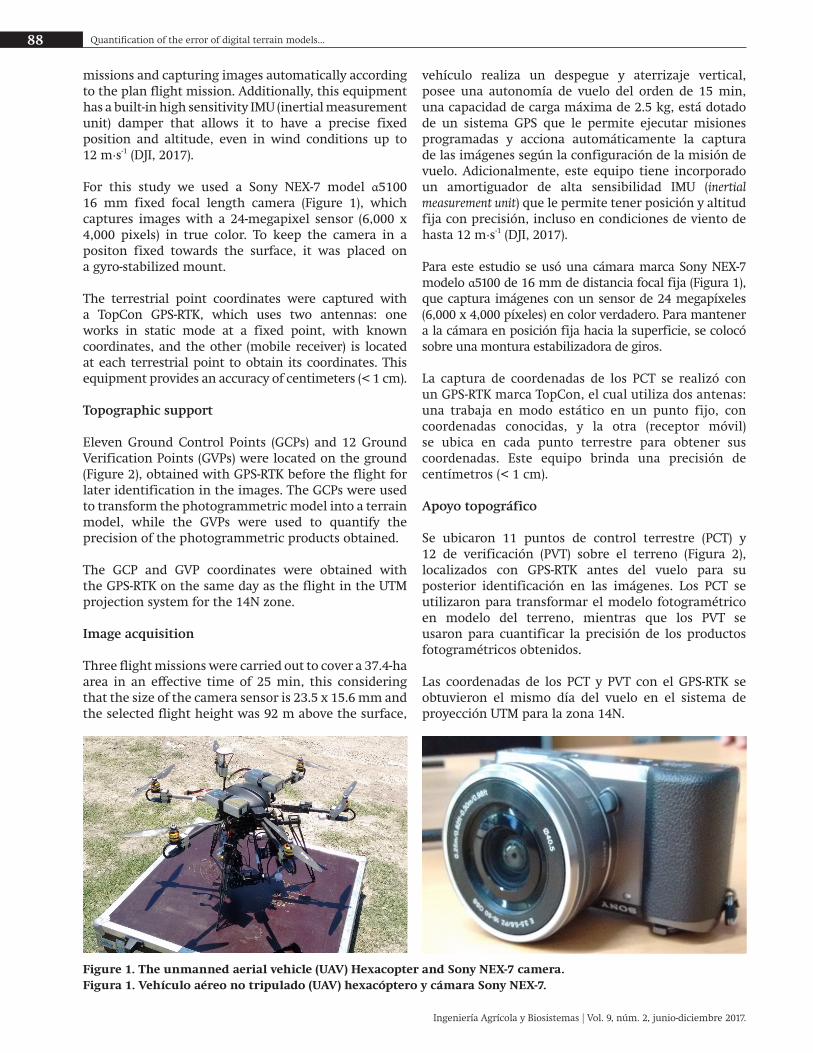
For this study we used a Sony NEX-7 model α5100 16 mm fixed focal length camera (Figure 1), which captures images with a 24-megapixel sensor (6,000 x 4,000 pixels) in true color. To keep the camera in a positon fixed towards the surface, it was placed on a gyro-stabilized mount.

The terrestrial point coordinates were captured with a TopCon GPS-RTK, which uses two antennas: one works in static mode at a fixed point, with known coordinates, and the other (mobile receiver) is located at each terrestrial point to obtain its coordinates. This equipment provides an accuracy of centimeters (< 1 cm).

Topographic support

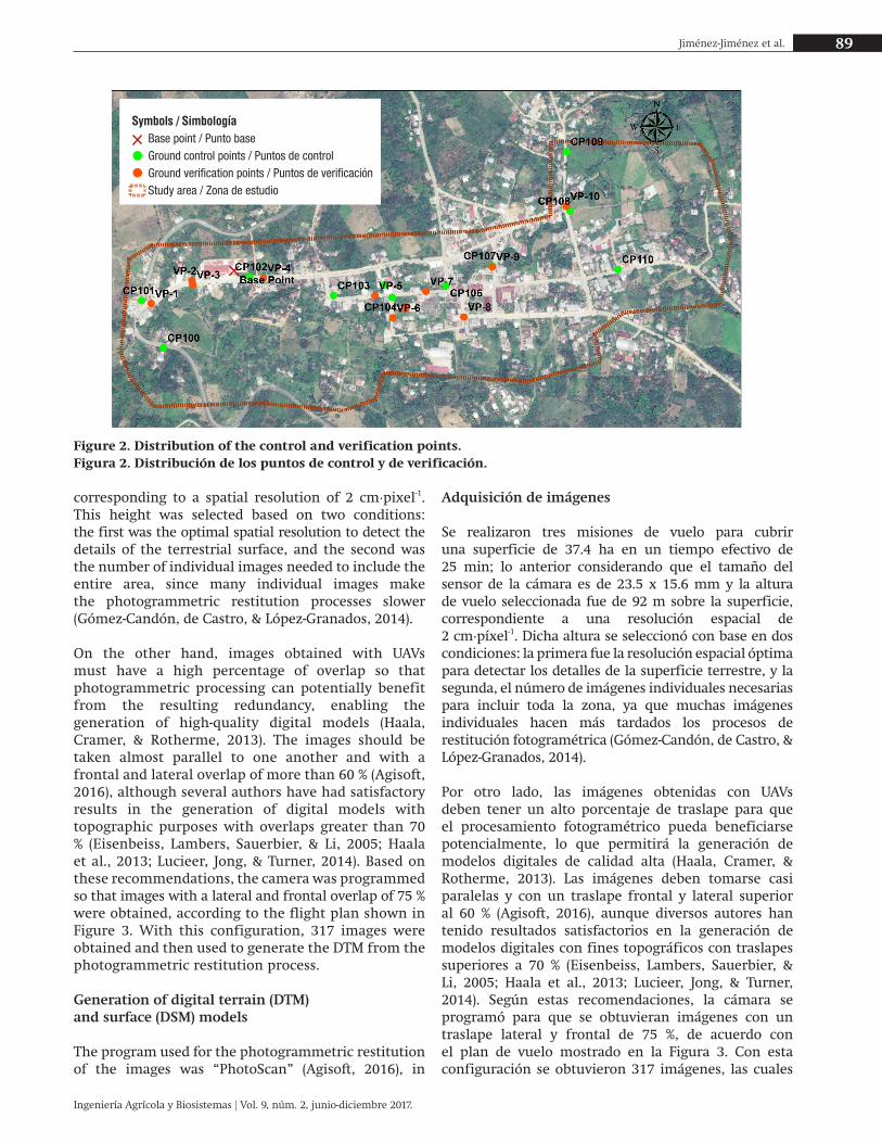
Eleven Ground Control Points (GCPs) and 12 Ground Verification Points (GVPs) were located on the ground (Figure 2), obtained with GPS-RTK before the flight for later identification in the images. The GCPs were used to transform the photogrammetric model into a terrain model, while the GVPs were used to quantify the precision of the photogrammetric products obtained.

The GCP and GVP coordinates were obtained with the GPS-RTK on the same day as the flight in the UTM projection system for the 14N zone.

Image acquisition

Three flight missions were carried out to cover a 37.4-ha area in an effective time of 25 min, this considering that the size of the camera sensor is 23.5 x 15.6 mm and the selected flight height was 92 m above the surface,

Figure 1. The unmanned aerial vehicle (UAV) Hexacopter and Sony NEX-7 camera.Figura 1. Vehículo aéreo no tripulado (UAV) hexacóptero y cámara Sony NEX-7.

vehículo realiza un despegue y aterrizaje vertical, posee una autonomía de vuelo del orden de 15 min, una capacidad de carga máxima de 2.5 kg, está dotado de un sistema GPS que le permite ejecutar misiones programadas y acciona automáticamente la captura de las imágenes según la configuración de la misión de vuelo. Adicionalmente, este equipo tiene incorporado un amortiguador de alta sensibilidad IMU (inertial measurement unit) que le permite tener posición y altitud fija con precisión, incluso en condiciones de viento de hasta 12 m∙s-1 (DJI, 2017).

Para este estudio se usó una cámara marca Sony NEX-7 modelo α5100 de 16 mm de distancia focal fija (Figura 1), que captura imágenes con un sensor de 24 megapíxeles (6,000 x 4,000 píxeles) en color verdadero. Para mantener a la cámara en posición fija hacia la superficie, se colocó sobre una montura estabilizadora de giros.

La captura de coordenadas de los PCT se realizó con un GPS-RTK marca TopCon, el cual utiliza dos antenas: una trabaja en modo estático en un punto fijo, con coordenadas conocidas, y la otra (receptor móvil) se ubica en cada punto terrestre para obtener sus coordenadas. Este equipo brinda una precisión de centímetros (< 1 cm).

Apoyo topográfico

Se ubicaron 11 puntos de control terrestre (PCT) y 12 de verificación (PVT) sobre el terreno (Figura 2), localizados con GPS-RTK antes del vuelo para su posterior identificación en las imágenes. Los PCT se utilizaron para transformar el modelo fotogramétrico en modelo del terreno, mientras que los PVT se usaron para cuantificar la precisión de los productos fotogramétricos obtenidos.

Las coordenadas de los PCT y PVT con el GPS-RTK se obtuvieron el mismo día del vuelo en el sistema de proyección UTM para la zona 14N.



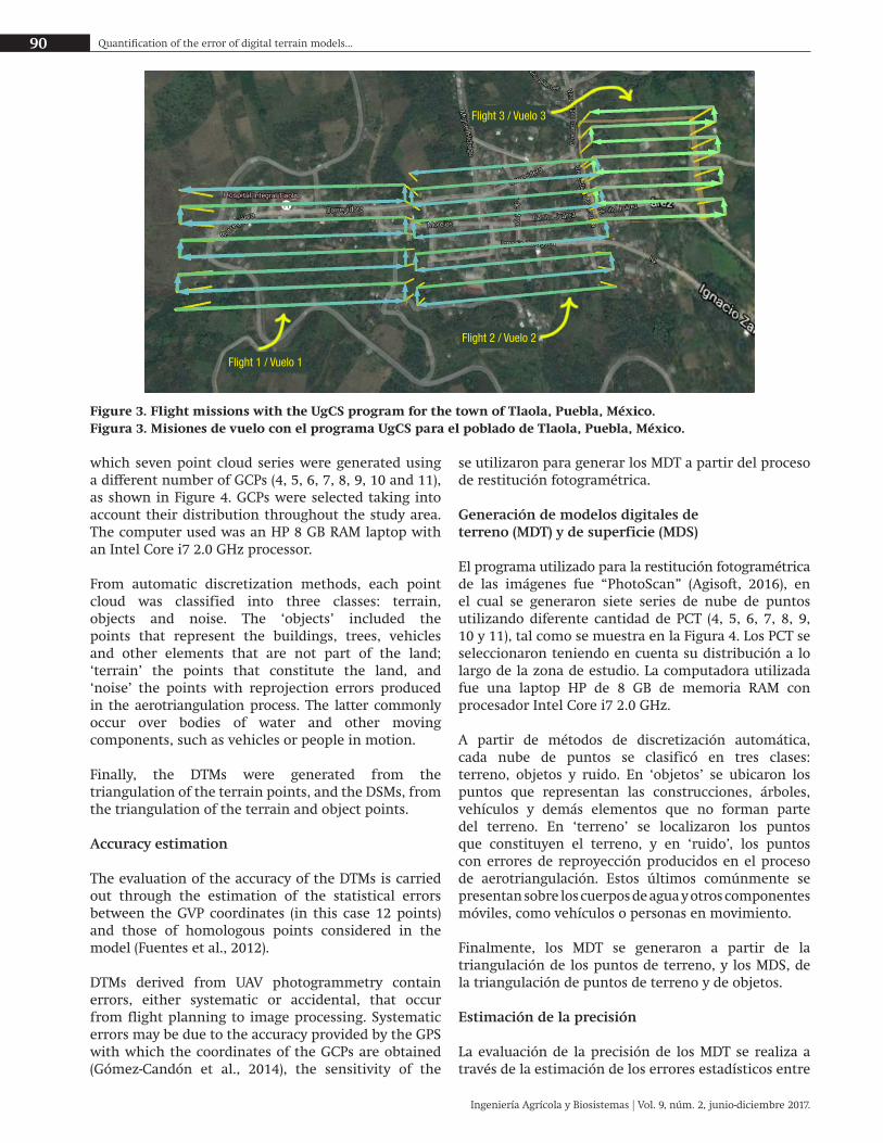
corresponding to a spatial resolution of 2 cm∙pixel-1. This height was selected based on two conditions: the first was the optimal spatial resolution to detect the details of the terrestrial surface, and the second was the number of individual images needed to include the entire area, since many individual images make the photogrammetric restitution processes slower (Gómez-Candón, de Castro, & López-Granados, 2014). On the other hand, images obtained with UAVs must have a high percentage of overlap so that photogrammetric processing can potentially benefit from the resulting redundancy, enabling the generation of high-quality digital models (Haala, Cramer, & Rotherme, 2013). The images should be taken almost parallel to one another and with a frontal and lateral overlap of more than 60 % (Agisoft, 2016), although several authors have had satisfactory results in the generation of digital models with topographic purposes with overlaps greater than 70 % (Eisenbeiss, Lambers, Sauerbier, & Li, 2005; Haala et al., 2013; Lucieer, Jong, & Turner, 2014). Based on these recommendations, the camera was programmed so that images with a lateral and frontal overlap of 75 % were obtained, according to the flight plan shown in Figure 3. With this configuration, 317 images were obtained and then used to generate the DTM from the photogrammetric restitution process.

Generation of digital terrain (DTM) and surface (DSM) models

The program used for the photogrammetric restitution of the images was “PhotoScan” (Agisoft, 2016), in

Symbols / SimbologíaBase point / Punto baseGround control points / Puntos de controlGround verification points / Puntos de verificaciónStudy area / Zona de estudio

Figure 2. Distribution of the control and verification points. Figura 2. Distribución de los puntos de control y de verificación.

Adquisición de imágenes

Se realizaron tres misiones de vuelo para cubrir una superficie de 37.4 ha en un tiempo efectivo de 25 min; lo anterior considerando que el tamaño del sensor de la cámara es de 23.5 x 15.6 mm y la altura de vuelo seleccionada fue de 92 m sobre la superficie, correspondiente a una resolución espacial de 2 cm∙píxel-1. Dicha altura se seleccionó con base en dos condiciones: la primera fue la resolución espacial óptima para detectar los detalles de la superficie terrestre, y la segunda, el número de imágenes individuales necesarias para incluir toda la zona, ya que muchas imágenes individuales hacen más tardados los procesos de restitución fotogramétrica (Gómez-Candón, de Castro, & López-Granados, 2014).

Por otro lado, las imágenes obtenidas con UAVs deben tener un alto porcentaje de traslape para que el procesamiento fotogramétrico pueda beneficiarse potencialmente, lo que permitirá la generación de modelos digitales de calidad alta (Haala, Cramer, & Rotherme, 2013). Las imágenes deben tomarse casi paralelas y con un traslape frontal y lateral superior al 60 % (Agisoft, 2016), aunque diversos autores han tenido resultados satisfactorios en la generación de modelos digitales con fines topográficos con traslapes superiores a 70 % (Eisenbeiss, Lambers, Sauerbier, & Li, 2005; Haala et al., 2013; Lucieer, Jong, & Turner, 2014). Según estas recomendaciones, la cámara se programó para que se obtuvieran imágenes con un traslape lateral y frontal de 75 %, de acuerdo con el plan de vuelo mostrado en la Figura 3. Con esta configuración se obtuvieron 317 imágenes, las cuales



which seven point cloud series were generated using a different number of GCPs (4, 5, 6, 7, 8, 9, 10 and 11), as shown in Figure 4. GCPs were selected taking into account their distribution throughout the study area. The computer used was an HP 8 GB RAM laptop with an Intel Core i7 2.0 GHz processor.

From automatic discretization methods, each point cloud was classified into three classes: terrain, objects and noise. The ‘objects’ included the points that represent the buildings, trees, vehicles and other elements that are not part of the land; ‘terrain’ the points that constitute the land, and ‘noise’ the points with reprojection errors produced in the aerotriangulation process. The latter commonly occur over bodies of water and other moving components, such as vehicles or people in motion.

Finally, the DTMs were generated from the triangulation of the terrain points, and the DSMs, from the triangulation of the terrain and object points.

Accuracy estimation

The evaluation of the accuracy of the DTMs is carried out through the estimation of the statistical errors between the GVP coordinates (in this case 12 points) and those of homologous points considered in the model (Fuentes et al., 2012).

DTMs derived from UAV photogrammetry contain errors, either systematic or accidental, that occur from flight planning to image processing. Systematic errors may be due to the accuracy provided by the GPS with which the coordinates of the GCPs are obtained (Gómez-Candón et al., 2014), the sensitivity of the

Figure 3. Flight missions with the UgCS program for the town of Tlaola, Puebla, México. Figura 3. Misiones de vuelo con el programa UgCS para el poblado de Tlaola, Puebla, México.

se utilizaron para generar los MDT a partir del proceso de restitución fotogramétrica.

Generación de modelos digitales de terreno (MDT) y de superficie (MDS)

El programa utilizado para la restitución fotogramétrica de las imágenes fue “PhotoScan” (Agisoft, 2016), en el cual se generaron siete series de nube de puntos utilizando diferente cantidad de PCT (4, 5, 6, 7, 8, 9, 10 y 11), tal como se muestra en la Figura 4. Los PCT se seleccionaron teniendo en cuenta su distribución a lo largo de la zona de estudio. La computadora utilizada fue una laptop HP de 8 GB de memoria RAM con procesador Intel Core i7 2.0 GHz.

A partir de métodos de discretización automática, cada nube de puntos se clasificó en tres clases: terreno, objetos y ruido. En ‘objetos’ se ubicaron los puntos que representan las construcciones, árboles, vehículos y demás elementos que no forman parte del terreno. En ‘terreno’ se localizaron los puntos que constituyen el terreno, y en ‘ruido’, los puntos con errores de reproyección producidos en el proceso de aerotriangulación. Estos últimos comúnmente se presentan sobre los cuerpos de agua y otros componentes móviles, como vehículos o personas en movimiento.

Finalmente, los MDT se generaron a partir de la triangulación de los puntos de terreno, y los MDS, de la triangulación de puntos de terreno y de objetos.

Estimación de la precisión

La evaluación de la precisión de los MDT se realiza a través de la estimación de los errores estadísticos entre

Flight 1 / Vuelo 1

Flight 2 / Vuelo 2

Flight 3 / Vuelo 3



UAV to the presence of wind (since it is not possible to ensure a regular overlap of the images), the ability of autonomous UAV piloting or the low quality of its sensors (this can randomly affect its altitude and location on the flight) (Nex & Remondino, 2014), the type of UAV selected (multirotor UAVs are more stable than fixed-wing ones) and the geometric accuracy of the camera caused by the distortion of the lens.

On the other hand, accidental errors may be due to the lack of calibration of the camera’s internal parameters

Figure 4. Location of ground control points (GCPs) by the photogrammetric restitution project.Figura 4. Ubicación de puntos de control terrestre (PCT) por proyecto de restitución fotogramétrica.

las coordenadas de PV (en este caso 12 puntos) y las coordenadas de puntos homólogos consideradas en el modelo (Fuentes et al., 2012).

Los MDT derivados de la fotogrametría con UAVs contienen errores, ya sea sistemáticos o accidentales, que ocurren desde la planificación del vuelo hasta el procesamiento de las imágenes. Los errores sistemáticos pueden deberse a la precisión que brinda el GPS con el que se obtiene las coordenadas de los PCT (Gómez-Candón et al., 2014) a la sensibilidad del UAV

A) 11 GCPs / 11 PCT

B) 10 GCPs / 10 PCT C) 9 GCPs / 9 PCT

D) 8 GCPs / 8 PCT E) 6 GCPs / 6 PCT

F) 5 GCPs / 5 PCT G) 4 GCPs / 4 PCT



(Nex & Remondino, 2014), the low percentage (< 70 %) of overlapping between images, the focus of the camera on the flight (since it may not stay fixed, which makes the focal distance vary) (Cabezos & Cisneros, 2012), the number of GCPs selected and their distribution in the field (Grenzdörffer, Engel, & Teichert, 2008), and poor identification of the GCPs in the images within the photogrammetric restitution program (Westoby, Brasington, Glasser, Hambrey, & Reynolds, 2012).

The accuracy of the DTMs was evaluated with the total errors, which involve the errors present from the planning of the flight until the generation of the models with the photogrammetric technique, for which four statistical error parameters were calculated (Equations 1 to 4): the mean error (ME), the root-mean-square error (RMSE), the standard deviation of the error (SDE) and the maximum absolute error (Emax). ME is a measure of the accuracy of the data that indicates any positive or negative systematic error, RMSE is a dispersion measure of the frequency distribution of the residuals that is sensitive to large errors, SDE provides information on the accuracy and distribution of the residuals around the average and Emax describes the greater residual present for understanding the quality limits of the data (Willmott & Matsuura, 2005). The residuals (Ccal-Cobs) on each axis were calculated as the difference between the measurements taken from the DTMs and those taken with the GPS-RTK on the plane (X, Y, Z) (Equation 5). Positive values indicate overestimation of data from the DTM, and negative values indicate underestimation of data by the DTM.

E= ni (Ccal – Cobs)

nM (1)

RMSE= n

i (Ccal-Cobs)2

n

(2)

SDE= ni [ Ccal-Cobs -ME]2

n-1 (3)

(4)Emax=max Ccal-Cobs

Ccal-Cobs= Xcal-Xobs2+ Ycal-Yobs

2 + Zcal-Zobs2 (5)

Where: Ccal = coordinates x, y, z extracted from the DTM in the GVPs and Cobs = coordinates of the GVPs measured with the GPS-RTK.

The SDE for each axis should not be understood as the maximum error of the DTM on that axis, but as an indicator of the overall error. Assuming a normal distribution of errors, 68.27 % of the errors are below the indicated SDE, 95.45 % twofold below the SDE and 99.76 % threefold below the SDE.

a la presencia de viento (ya que no se puede asegurar un traslape regular de las imágenes), a la capacidad de pilotaje autónomo del UAV o calidad baja de sus sensores (esto puede afectar aleatoriamente su altitud y ubicación en el vuelo) (Nex & Remondino, 2014), al tipo de UAV seleccionado (los multirotores son más estables que los de ala fija) y a la precisión geométrica de la cámara provocada por la distorsión del objetivo.

Por otro lado, los errores accidentales pueden deberse a la falta de calibración de los parámetros internos de la cámara (Nex & Remondino, 2014), al porcentaje bajo (< 70 %) de traslape entre imágenes, al enfoque de la cámara en el vuelo (ya que puede que no se mantenga fijo, lo que hace que la distancia focal varíe) (Cabezos & Cisneros, 2012), al número de PCT seleccionados y a su distribución en el terreno (Grenzdörffer, Engel, & Teichert, 2008) y a la deficiente identificación de los PCT en las imágenes dentro del programa de restitución fotogramétrica (Westoby, Brasington, Glasser, Hambrey, & Reynolds, 2012). La evaluación de la precisión de los MDT se realizó con los errores totales, los cuales involucran los errores presentes desde la planificación del vuelo hasta la generación de los modelos con la técnica fotogramétrica, para ello se calcularon cuatro parámetros estadísticos de error (Ecuaciones 1 a 4): el error medio (EM), la raíz del cuadrado medio del error (RCME), la desviación estándar de los errores (DEE) y el error absoluto máximo (Emáx). El EM es una medida de precisión de los datos que indica cualquier error sistemático positivo o negativo, la RCME es una medida de dispersión de la distribución de frecuencias de los residuales que es sensible a grandes errores, la DEE proporciona información sobre la precisión y distribución de los residuos alrededor de la media y el Emáx describe el residual mayor presente para la comprensión de los límites de la calidad de los datos (Willmott & Matsuura, 2005). Los residuales (Ccal-Cobs) en cada eje se calcularon como la diferencia entre las mediciones extraídas de los MDT y las tomadas con el GPS-RTK en el plano (X, Y, Z) (Ecuación 5). Los valores positivos indican sobreestimación de datos del MDT, y los negativos, subestimación de datos por parte del MDT. EM=

ni (Ccal – Cobs)

n (1)

RCME=

ni (Ccal-Cobs)

2

n (2)

DEE= ni [ Ccal-Cobs -EM]2

n-1(3)

(4)Emax=max Ccal-Cobs

Ccal-Cobs= Xcal-Xobs2+ Ycal-Yobs

2 + Zcal-Zobs2 (5)



Results and discussion

Generation of DTM and DSM

For each of the seven photogrammetric restitutions, a dense cloud of points, a DSM, a DTM and an orthomosaic were obtained; the main characteristics of these photogrammetric products are shown in Table 1.

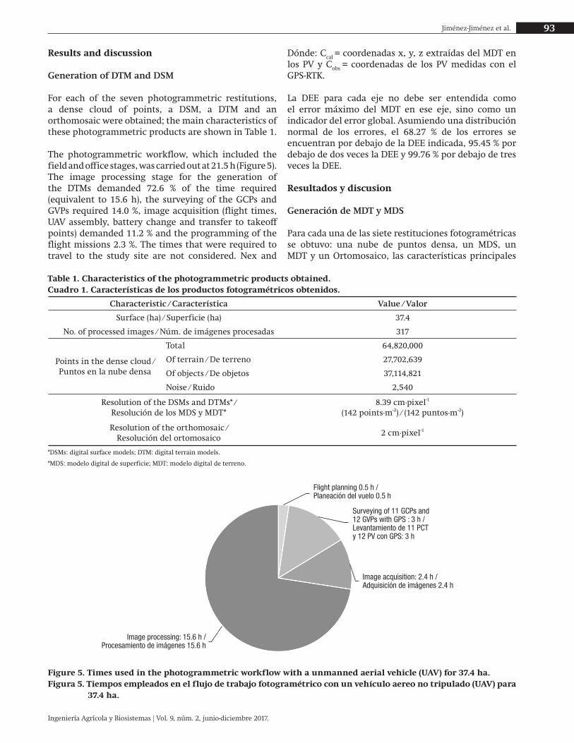
The photogrammetric workflow, which included the field and office stages, was carried out at 21.5 h (Figure 5). The image processing stage for the generation of the DTMs demanded 72.6 % of the time required (equivalent to 15.6 h), the surveying of the GCPs and GVPs required 14.0 %, image acquisition (flight times, UAV assembly, battery change and transfer to takeoff points) demanded 11.2 % and the programming of the flight missions 2.3 %. The times that were required to travel to the study site are not considered. Nex and

Table 1. Characteristics of the photogrammetric products obtained.Cuadro 1. Características de los productos fotogramétricos obtenidos.

Characteristic / Característica Value / Valor

Surface (ha) / Superficie (ha) 37.4

No. of processed images / Núm. de imágenes procesadas 317

Points in the dense cloud /Puntos en la nube densa

Total 64,820,000

Of terrain / De terreno 27,702,639

Of objects / De objetos 37,114,821

Noise / Ruido 2,540

Resolution of the DSMs and DTMs* /Resolución de los MDS y MDT*

8.39 cm∙pixel-1 (142 points∙m-2) / (142 puntos∙m-2)

Resolution of the orthomosaic /Resolución del ortomosaico

2 cm∙pixel-1

*DSMs: digital surface models; DTM: digital terrain models.

*MDS: modelo digital de superficie; MDT: modelo digital de terreno.

Figure 5. Times used in the photogrammetric workflow with a unmanned aerial vehicle (UAV) for 37.4 ha.Figura 5. Tiempos empleados en el flujo de trabajo fotogramétrico con un vehículo aereo no tripulado (UAV) para

37.4 ha.

Dónde: Ccal = coordenadas x, y, z extraídas del MDT en los PV y Cobs = coordenadas de los PV medidas con el GPS-RTK.

La DEE para cada eje no debe ser entendida como el error máximo del MDT en ese eje, sino como un indicador del error global. Asumiendo una distribución normal de los errores, el 68.27 % de los errores se encuentran por debajo de la DEE indicada, 95.45 % por debajo de dos veces la DEE y 99.76 % por debajo de tres veces la DEE.

Resultados y discusion

Generación de MDT y MDS

Para cada una de las siete restituciones fotogramétricas se obtuvo: una nube de puntos densa, un MDS, un MDT y un Ortomosaico, las características principales

Flight planning 0.5 h /Planeación del vuelo 0.5 h

Surveying of 11 GCPs and 12 GVPs with GPS : 3 h / Levantamiento de 11 PCTy 12 PV con GPS: 3 h

Image acquisition: 2.4 h / Adquisición de imágenes 2.4 h

Image processing: 15.6 h / Procesamiento de imágenes 15.6 h



Remondino (2014) mention that the image processing stage requires the most time in photogrammetric work with UAV, approximately 60 %; although in this work it was greater, it can be improved if a computer with a greater processing capacity is used.

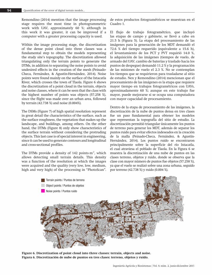
Within the image processing stage, the discretization of the dense point cloud into three classes was a fundamental step to obtain the models representing the study site’s topography. The discretization allowed triangulating only the terrain points to generate the DTMs, in addition to separating the noise points to avoid undesired effects in the creation of the mesh (Peinado-Checa, Fernández, & Agustín-Hernández, 2014). Noise points were found mainly on the surface of the Ixtacatla River, which crosses the town of Tlaola. Figure 6 shows the discretization of a point cloud in the terrain, objects and noise classes, where it can be seen that the class with the highest number of points was objects (57.258 %), since the flight was made over an urban area, followed by terrain (42.738 %) and noise (0.004%).

The DSMs (Figure 7) of high spatial resolution represent in great detail the characteristics of the surface, such as the surface roughness, the vegetation that makes up the landscape, and buildings, among others. On the other hand, the DTMs (Figure 8) only show characteristics of the surface terrain without considering the protruding objects. This last case is of special interest in engineering, since it can be used to generate contours and longitudinal and cross-sectional profiles.

The DTMs provide a density of 142 points∙m-2, which allows detecting small terrain details. This density was a function of the resolution at which the images were acquired and the quality (very low, low, medium, high and very high) of the processing in “PhotoScan”.

Figure 6. Discretization of point cloud into three classes: terrain, objects and noise.Figura 6. Discretización de nube de puntos en tres clases: terreno, objetos y ruido.

de estos productos fotogramétricos se muestran en el Cuadro 1.

El flujo de trabajo fotogramétrico, que incluyó las etapas de campo y gabinete, se llevó a cabo en 21.5 h (Figura 5). La etapa del procesamiento de las imágenes para la generación de los MDT demandó el 72.6 % del tiempo requerido (equivalente a 15.6 h), el levantamiento de los PCT y PVT requirió 14.0 %, la adquisición de las imágenes (tiempos de vuelo, de armado del UAV, cambio de baterías y traslado hacia los puntos de despegue) demandó 11.2 % y la programación de las misiones de vuelo el 2.3 %. No se contemplan los tiempos que se requirieron para trasladarse al sitio de estudio. Nex y Remondino (2014) mencionan que el procesamiento de las imágenes es la etapa que requiere mayor tiempo en trabajos fotogramétricos con UAVs, aproximadamente 60 %; aunque en este trabajo fue mayor, puede mejorarse si se ocupa una computadora con mayor capacidad de procesamiento.

Dentro de la etapa de procesamiento de las imágenes, la discretización de la nube de puntos densa en tres clases fue un paso fundamental para obtener los modelos que representan la topografía del sitio de estudio. La discretización permitió triangular únicamente los puntos de terreno para generar los MDT, además de separar los puntos ruido para evitar efectos indeseados en la creación de la malla (Peinado-Checa, Fernández, & Agustín-Hernández, 2014). Los puntos ruido se encontraron principalmente sobre la superficie del río Ixtacatla, el cual atraviesa el poblado de Tlaola. En la Figura 6 se muestra la discretización de una nube de puntos en las clases terreno, objetos y ruido, donde se observa que la clase con mayor número de puntos fue objetos (57.258 %), ya que el vuelo se realizó sobre una zona urbana, seguido por terreno (42.738 %) y ruido (0.004 %).

Terrain points / Puntos de terreno

Object points / Puntos de objetos

Noise points / Puntos ruido



Figure 7. Digital surface model (DSM).Figura 7. Modelo digital de superficie (MDS).

Figure 8. Digital terrain model (DTM). Figura 8. Modelo digital de terreno (MDT).

Generally, this type of technology can provide a density greater than 100 points∙m-2 (Cryderman, Bill-Mah, & Shufletoski, 2015; Neitzel & Klonowski, 2012) in a relatively short time, which could not be achieved with conventional technologies such as total station or GPS.

Accuracy estimation

The ME of the DTM generated with four GCPs was less than 11 cm on the X and Y axes, while on Z it was greater than 2 m. This DTM greatly overestimated terrain elevations, indicating that the number of GCPs used for its georeferencing are not sufficient; however, the errors in X and Y are not so large because the percentage of overlap between images had a greater influence than the number of GCPs. For the rest of the DTMs, the ME values on the three axes were less than 2 cm, which shows that the number of points and their distribution are important in determining the accuracy of the models, since GCPs were used in the corners and near the center of the study area.

Los MDS (Figura 7) de alta resolución espacial representan con gran detalle las características de la superficie, como rugosidad del terreno, vegetación que compone el paisaje, construcciones, entre otros. Por otro lado, los MDT (Figura 8) solo muestran características del terreno superficial sin considerar los objetos sobresalientes. Este último caso es de especial interés en ingeniería, ya que puede ser utilizado para generar curvas de nivel, perfiles longitudinales y trasversales.

Los MDT brindan una densidad de 142 puntos∙m-2, lo que permite detectar pequeños detalles del terreno. Dicha densidad estuvo en función de la resolución a la que se adquirieron las imágenes y de la calidad (muy baja, baja, media, alta y muy alta) del procesamiento en “PhotoScan”. Generalmente, este tipo de tecnologías pueden brindar densidad mayores a 100 puntos∙m-2

(Cryderman, Bill-Mah, & Shufletoski, 2015; Neitzel & Klonowski, 2012) en tiempos relativamente cortos, lo cual no se podría lograr con las tecnologías convencionales como estación total o GPS.



In the analyses with the RMSE, it was found that the DTMs have a greater error on vertical (Z) than horizontal (X and Y) axes. The DTM with four GCPs has a value greater than 3 m on the Z axis, and with five or more GCPs have errors of less than 5, 4 and 12 cm on the X, Y and Z axes, respectively. This again highlights the importance of having GCPs in the central area of the study area. The RMSE, in comparison with the ME, amplifies and penalizes with greater force those errors of greater magnitude.

In these digital models, as errors are greater in the vertical than in the horizontal, several authors have quantified the error only on the vertical axis with the support of a multirotor UAV, finding an RMSE of 8.8 cm (Tamminga et al., 2014) and 6.6. cm (Uysal, Toprak, & Polat, 2015), while Hugenholtz et al. (2013), when using a fixed-wing UAV, obtained an RMSE of 29 cm. This shows that the accuracy on the three axes of the digital models generated by photogrammetry using UAV can be less than 10 cm. Nex and Remondino (2014) mention that the RMSE of these models is generally two to three times the pixel size of the acquired images (or the spatial resolution of the orthomosaic). In this case, the georeferenced models with 9, 10 and 11 GCPs have an RMSE of less than 10 cm in the three axes; however, only the model georeferenced with 11 GCPs has an RMSE (5.9 cm) of less than three times the resolution of the orthomosaic (2 cm∙pixel-1). Therefore, the latter could represent the site’s topography with high accuracy.

Because the DTM referenced with 11 GCPs is the one with the best accuracy and the one that best represents the site’s topography, according to the SDE, the accuracy on the Z axis was less than 5.8 cm in 25.53 ha (68.27 % of the total surface), 11.6 cm in 35.70 ha (95.45 %) and 17 cm in 37.31 ha.

The Emax, like the other estimators, was greater on the Z axis. The Emax that was found in all the DTMs on the plane (X, Y, Z) was in GVP 10, because it is located in an area (near the edge) with less than six overlapping images, while the other points present at least nine images for photogrammetric restitution. In photogrammetric surveys near the edge of the surveyed area, the number of overlapping images is smaller with respect to the central area; therefore, it is advisable to program the flight mission for a larger area of the area of interest, in such a way that a minimum number of overlapping images (nine) images is ensured. On the other hand, one should avoid locating terrestrial points near the boundaries of the area of interest.

Table 2 shows the comparison of the errors calculated for the DTMs generated from different CP numbers. The statistical errors of the digital models on the plane (X, Y, Z) (Figure 9) decreased when the number of GCPs

Estimación de la precisión

El EM del MDT generado con cuatro PCT fue inferior a 11 cm en los ejes X y Y, en tanto que en Z fue superior a 2 m. Este MDT sobreestimó en gran medida las elevaciones del terreno, lo que indica que el número de PCT utilizados para su georeferenciación no son suficientes; sin embargo, los errores en X y Y no logran ser tan grandes debido a que influyó más el porcentaje de traslape entre imágenes que el número de PCT. Para el resto de los MDT, los valores del EM en los tres ejes fueron inferiores a 2 cm, lo cual muestra que el número de puntos y su distribución son importantes para determinar la precisión de los modelos, ya que se usaron PC en las esquinas y cerca del centro de la zona de estudio.

En los análisis con la RCME se encontró que los MDT presentan un error mayor en vertical (Z) que en horizontal (X y Y). El MDT con cuatro PCT presenta un valor mayor a 3 m en el eje Z, y con cinco o más PCT presentan errores menores de 5, 4 y 12 cm en los ejes X, Y y Z, respectivamente. Esto vuelve a resaltar la importancia de contar con PCT en la zona central del área de estudio. La RCME, en comparación con el EM, amplifica y penaliza con mayor fuerza aquellos errores de mayor magnitud.

En estos modelos digitales, al ser mayores los errores en el vertical que en el horizontal, diversos autores han cuantificado el error únicamente en el eje vertical con el apoyo de un UAV multirotor, encontrando una RCME de 8.8 cm (Tamminga et al., 2014) y de 6.6. cm (Uysal, Toprak, & Polat, 2015); mientras que Hugenholtz et al. (2013), al utilizar un UAV de ala fija, obtuvieron una RCME de 29 cm. Lo anterior muestra que la precisión en los tres ejes de los modelos digitales generados por fotogrametría con UAVs puede llegar a ser menor de 10 cm. Nex y Remondino (2014) mencionan que la RCME de estos modelos generalmente es de dos a tres veces el tamaño del pixel de las imágenes adquiridas (o de la resolución espacial del ortomosaico). En este caso, los modelos georreferenciados con 9, 10 y 11 PCT tienen RCME menores a 10 cm en los tres ejes; sin embargo, únicamente el georreferenciado con 11 PCT tiene un RCME (5.9 cm) menor de tres veces la resolución del ortomosaico (2 cm∙pixel-1). Por lo tanto, este último podría representar con alta precisión la topografía del sitio.

Debido a que el MDT referenciado con 11 PC es el de mejor precisión y el que representa mejor la topografía del sitio, de acuerdo con la DEE, la precisión en el eje Z fue menor de 5.8 cm en 25.53 ha (68.27 % de la superficie total), 11.6 cm en 35.70 ha (95.45 %) y 17 cm en 37.31 ha.

El Emáx, al igual que los demás estimadores, fue mayor en el eje Z. El Emáx que se encontró en todos los MDT



used for their georeferencing increased. The accuracy of digital models on X and Y remains stable (RMSE < 5 cm) from five GCPs, while on the Z axis a greater influence of the number of points is observed, since the values of the RMSE were found to be greater than 10 cm when less than nine points were used.

Table 2. Comparison of statistical errors between digital terrain models and GPS-RTK measurements.Cuadro 2. Comparación de errores estadísticos entre los modelos digitales de terreno y las mediciones del GPS-RTK.

Axis / EjeParameters (cm) /Parámetros (cm)

Number of ground control points /Número de puntos de control

4 5 6 8 9 10 11

X ME* / EM* 6.5 -0.4 1.7 0.5 0.0 -0.1 0.3

RMSE / RCME 9.4 4.3 5.2 3.0 3.7 3.7 2.1

SDE / DEE 7.1 4.5 5.1 3.0 3.8 3.8 2.2

Emax 16.2 9.4 10.9 5.3 7.4 10.2 4.1

Y ME* / EM* 10.5 0.0 0.9 0.6 -0.1 0.0 1.3

RMSE / RCME 11.6 3.2 3.0 2.7 3.3 3.8 3.0

SDE / DEE 6.8 3.4 3.0 2.7 3.4 3.9 2.8

Emax 17.8 6.0 6.4 5.8 6.2 7.4 6.9

Z ME* / EM* 275.5 0.0 1.5 1.2 0.3 -0.6 2.1

RMSE / RCME 304.1 12.2 11.2 10.5 7.7 6.6 5.9

SDE / DEE 134.5 12.8 11.6 10.9 8.0 6.9 5.8

Emax 400.7 30.0 29.0 27.0 18.0 12.2 10.9

Average(X, Y, Z) /

Promedio(X, Y, Z)

ME* / EM* 276.0 10.9 10.0 9.0 7.6 7.5 6.2

RMSE / RCME 304.5 13.4 12.7 11.2 9.1 8.5 7.0

SDE / DEE 134.2 8.2 8.1 7.1 5.2 4.2 3.2

Emax 401.2 32.0 31.3 27.7 20.3 14.4 11.7

*ME: mean error; RMSE: root-mean-square error; SDE: standard deviation of the error; Emax: maximum absolute error.

*EM: error medio; RCME: raíz del cuadrado medio del error; DEE: desviación estándar de los errores; Emáx: error absoluto máximo.

Figure 9. Statistical errors of the digital terrain models on the plane (X, Y, Z). *ME: mean error; RMSE: root-mean-square error; Emax: maximum absolute error.Figura 9. Errores estadísticos de los modelos digitales de terreno en el plano (X, Y, Z). *EM: error medio; RCME: raíz del cuadrado medio del error; Emáx: error absoluto máximo.

en el plano (X, Y, Z) fue en el PV 10, debido a que se ubica en una zona (cerca del borde) con menos de seis imágenes traslapadas, mientras que los demás puntos presentan al menos nueve imágenes para la restitución fotogramétrica. En los levantamientos fotogramétricos cerca del borde del área levantada, el número de

Errors on the plane (X, Y, Z) / Errores en el plano (X, Y, Z)

Erro

r (cm

)

ME / EM RMSE / RCME Emax

Number of ground control points / Número de puntos de control



The results show that accuracy of less than 10 cm (in the three axes) can be obtained in the DTMs derived from photogrammetry with UAV. This accuracy is greater than that obtained with other remote sensing technologies, as is the case of Fuentes et al. (2012), who used IKONOS satellite images and found accuracies of 1.49, 3.5 and 3.89 m on the X, Y and Z axes, respectively. On the other hand, Zhang, Pateraki, and Baltsavias (2002) obtained five DEMs with five different interpolation algorithms using IKONOS images and found RMSE values on the Z axis from 3.1 m to 5.4 m. With airborne LiDAR sensors, Bowen and Waltermire (2002) report an RMSE in the vertical of 43 cm, Legleiter (2012) of 21 cm and Notebaert, Verstraeten, Govers, and Poesen (2009) of 15 cm in the Belgian river valleys. However, there are other technologies such as terrestrial laser scanners that can provide accuracies of the order of 4 cm on Z (Williams et al., 2013), although with a cost of resources and time greater than with the use of UAVs.

Conclusions

Information capture by UAVs allows generating a greater number of points, which improves the level of detail with which the surface is represented in the models. The DTMs generated have a spatial resolution of 8.4 cm∙pixel-1, equivalent to 142 points∙m-2, and provide a level of detail that is not possible to obtain with traditional topographic equipment.

The most reliable statistical parameter to determine the accuracy of the models is the RMSE since it is sensitive to large errors. In turn, the ME estimator provides useful information, but it is not recommended when large-magnitude errors occur.

The largest errors in the DTMs were found on the Z axis. The number of GCPs in the terrain had a considerable impact on the accuracy of the DTMs, especially on the Z axis; that is, if the number of GCPs is low, accuracy is guaranteed on X and Y, but not on Z. The RMSEs on X and Y of the DTMs georeferenced with more than five GCPs were less than 5 cm, which shows little influence of the number of GCPs on the accuracy on these axes, while on Z they were greater than 10 cm when less than nine points were used.

The DTM georeferenced with 11 GCPs represented the site’s topography with better accuracy, since the highest RMSE, which was presented on the Z axis, was 5.9 cm, which is three times less than the spatial resolution of the orthomosaic (2 cm∙pixel-1). Therefore, at least five terrestrial GCPs well-distributed throughout the study area are essential for every 15 ha of surveyed surface; in addition, it is necessary to add one point for each additional 3 ha to obtain a minimum accuracy (RMSE) of 6 cm on the Z axis and 7 cm on the plane (X, Y, Z).

imágenes traslapadas es menor con respecto a la zona central; por tanto, es conveniente que la misión de vuelo se programe para una superficie mayor de la zona de interés, de tal manera que se garantice una cantidad mínima de imágenes (nueve) traslapadas. Por otro lado, se debe evitar ubicar puntos terrestres cercanos a los límites de la zona de interés.

En el Cuadro 2 se observa la comparación de los errores calculados para los MDT generados a partir de diferente número de PCT. Los errores estadísticos de los modelos digitales en el plano (X, Y, Z) (Figura 9) disminuyeron cuando aumentó el número de PCT utilizados para su georreferenciación. La precisión de los modelos digitales en X y Y se mantiene estable (RCME < 5 cm) a partir de cinco PCT; mientras que en el eje Z se observa una mayor influencia del número de puntos, ya que los valores de la RCME resultaron ser mayores a 10 cm cuando se utilizaron menos de nueve puntos.

Los resultados muestran que se puede obtener precisión menor a 10 cm (en los tres ejes) en los MDT derivados de la fotogrametría con UAVs. Dicha precisión es mayor que la obtenida con otras tecnologías de percepción remota, como es el caso de Fuentes et al. (2012), quienes usaron imágenes de satélite IKONOS y encontraron precisiones de 1.49, 3.5 y 3.89 m en los ejes X, Y y Z, respectivamente. Por otro lado, Zhang, Pateraki, y Baltsavias (2002) obtuvieron cinco MDE con cinco diferentes algoritmos de interpolación usando imágenes IKONOS y encontraron valores de la RCME, en el eje Z, desde 3.1 m hasta 5.4 m. Con sensores LiDAR aerotransportado, Bowen y Waltermire (2002) reportan una RCME en el vertical de 43 cm, Legleiter (2012) de 21 cm y Notebaert, Verstraeten, Govers, y Poesen (2009) de 15 cm en los valles fluviales belgas. No obstante, existen otras tecnologías como los escáneres laser terrestres que pueden proporcionar precisiones del orden de 4 cm en Z (Williams et al., 2013), aunque con un costo de recursos y tiempo mayor que con el empleo de UAVs.

Conclusiones

La captura de información mediante UAVs permite generar una mayor cantidad de puntos, lo que mejora el nivel del detalle con el que se representa la superficie en los modelos. Los MDT generados presentan una resolución espacial de 8.4 cm∙píxel-1, equivalente a 142 puntos∙m-2, y brindan un nivel de detalle que no es posible obtener con equipos topográficos tradicionales.

El parámetro estadístico más confiable para determinar la precisión de los modelos es la RCME ya que es sensible a grandes errores. A su vez, el estimador EM brinda información útil, pero no es recomendable cuando se presentan errores de gran magnitud.



Additionally, the frontal and lateral overlap of the images play an important role, since they determine the number of images in which the same point is observed. A minimum average frontal and lateral overlap of 75 % ensures an adequate number of points in the DTM. In addition, the flight mission must be programmed for a larger area of the area of interest, since near the limits of the flight area where few images overlap, the accuracy is less than in the central areas.

Finally, we were able to determine that the digital models derived from UAV photogrammetry are of high spatial resolution and can provide accuracies of less than 10 cm on the three axes. Therefore, this technology can be adopted in the field of topography, since these models are also obtained in shorter times and with fewer resources than conventional technologies such as total stations and differential GPS. However, both technologies should be considered complementary, because it is essential to obtain terrestrial GCPs for the georeferencing of digital models.

End of English version

References / Referencias

Agisoft. (2016). Agisoft PhotoScan user manual: professional edition, version 1.2. San Petersburgo, Rusia: Author.

Bowen, Z., & Waltermire, R. (2002). Evaluation of light detection and ranging (LIDAR) for measuring river corridor topography. Journal of the American Water Resources, 38(1), 33-41. doi: 10.1111/j.1752-1688.2002.tb01532.x

Cabezos, P., & Cisneros, J. (2012). Fotogrametría con cámaras digitales convencionales y software libre. Revista de Expresión Gráfica Arquitectónica, 20(1), 88-99. doi: 10.4995/ega.2012.1407

Cavallini, R., Mancini, F., & Zanni, M. (2004). Orthorectification of HR satellite images with space derived DSM. XXth Congress International Archives of Photogrammetry and Remote (pp. 1682-1700). Retrieved from http://www.isprs.org/proceedings/XXXV/congress/comm7/papers/201.pdf

Cryderman, C., Bill-Mah, S., & Shufletoski, A. (2015). Evaluation of UAV photogrammetric accuracy for mapping and earthworks computations. Geomática, 68(4), 309-317. doi: 10.5623/cig2014-405

DJI. (2017). A2 Especificaciones. Retrieved from http://www.dji.com/es/a2

Eisenbeiss, H., Lambers, K., Sauerbier, M., & Li, Z. (2005). Photogrammetric documentation of an archaeological site (Palpa, Peru) using an autonomous model helicopter. Proceedings of the XX International Symposium CIPA, 1-6. Retrieved from https://www.uni-bamberg.de/fileadmin/ivga/Lambers/eisenbeiss_et_al_2005.pdf

Flener, C., Vaaja, M., Jaakkola, A., Krooks, A., Kaartinen, H., Kukko, A., Kasvi, E., Hyyppä, H., Hyyppä, J., & Alho,

Los errores más grandes en los MDT se encontraron en el eje Z. El número de PCT influyó considerablemente en la precisión de los MDT, sobre todo en el eje Z; es decir, si el número de PCT es bajo se garantiza precisión en X y Y, pero no en Z. Las RCME en X y Y de los MDT georreferenciados con más de cinco PC fueron menor a 5 cm, lo cual muestra poca influencia de la cantidad de PCT sobre la precisión en estos ejes; mientras que en Z fueron mayores a 10 cm cuando se utilizaron menos de nueve puntos.

El MDT georreferenciado con 11 PC representó con mejor precisión la topografía del sitio, ya que la mayor RMSE, que se presentó en el eje Z, fue de 5.9 cm, la cual es menor a tres veces la resolución espacial del ortomosaico (2 cm∙pixel-1). Por lo tanto, son indispensables al menos cinco PCT bien distribuidos a lo largo de la zona de estudio por cada 15 ha de superficie levantada; además, es necesario agregar un punto por cada 3 ha adicionales para obtener una precisión (RCME) mínima de 6 cm en el eje Z y de 7 cm en el plano (X, Y, Z).

Adicionalmente, el traslape frontal y lateral de las imágenes juegan un papel importante, ya que determinan el número de imágenes en que se observa un mismo punto. Un traslape frontal y lateral promedio mínimo de 75 % garantiza una cantidad de puntos adecuada en el MDT. Además, la misión de vuelo debe programarse para una superficie mayor de la zona de interés, ya que cerca de los límites del área de vuelo en donde se traslapan pocas imágenes la precisión es menor que en las zonas centrales.

Finalmente, se pudo identificar que los modelos digitales derivados de la fotogrametría con UAVs son de alta resolución espacial y pueden brindan precisiones menores a 10 cm en los tres ejes. Por ello, esta tecnología puede ser adoptada en el campo de la topografía, ya que además estos modelos se obtienen en tiempos más cortos y con menos recursos que las tecnologías convencionales como estaciones totales y GPS diferenciales. Sin embargo, ambas tecnologías deben considerarse complementarias, debido a que es indispensable la toma de PCT para la georeferenciación de los modelos digitales.

Fin de la version en español

P. (2013). Seamless mapping of river channels at high resolution using mobile LiDAR and UAV-Photography. Remote Sensing, 5(1), 6382-6407. doi: 10.3390/rs5126382

Fuentes, J., Bolaños, J., & Rozo, D. (2012). Modelo digital de superficie a partir de imágenes de satélite IKONOS para el análisis de áreas de inundación en santa marta, Colombia. Boletín de Investigaciones Marinas y Costeras, 41(2), 251-266.



Gómez-Candón, D., de Castro, A. I., & López-Granados, F. (2014). Assessing the accuracy of mosaics from unmanned aerial vehicle (UAV) imagery for precision agriculture purposes in wheat. Precision Agriculture, 15(1), 44-56. doi: 10.1007/s11119-013-9335-4

Goncalves, J., & Henriques, R. (2015). UAV photogrammetry for topographic monitoring of coastal areas. Journal of Photogrammetry and Remote Sensing, 104, 101-111. doi: 10.1016/j.isprsjprs.2015.02.009

Grenzdörffer, G. J., Engel, A., & Teichert, B. (2008). The photogrammetric potential of low-cost UAVs in forestry and agriculture. The International Archives of the Photogrammetry, Remote Sensing and Spatial Information Sciences, Vol. XXXVII, 1207-2014. Retrieved from http://www.isprs.org/proceedings/XXXVII/congress/1_pdf/206.pdf

Haala, N., Cramer, M., & Rotherme, M. (2013). Quality of 3d point clouds from highly overlapping UAV imagery. International Archives of the Photogrammetry, Remote Sensing and Spatial Information Sciences, 40(1), 183-188.

Fook, H. (2008). 3D Terrestrial Laser Scanning for Application in Earthwork and Topographical Surveys (Bachelor thesis). University of Southern Queensland, Faculty of Engineering and Surveying, Australia.

Hernández, D. (2006). Introducción a la fotogrametría digital. Madrid, España: Universidad de Castilla la Mancha.

Hugenholtz, C. H., Whitehead, K., Brown, O. W., Barchyn, T. E., Moorman, B., LeClair, A., Riddell, K., & Hamilton, T. (2013). Geomorphological mapping with a small unmanned aircraft system (sUAS): Feature detection and accuracy assessment of a photogrammetrically-derived digital terrain model. Geomorphology, 194, 16-24. doi: 10.1016/j.geomorph.2013.03.023

Legleiter, C. (2012). Remote measurement of river morphology via fusion of LiDAR topography and spectrally based bathymetry. Earth Surface Processes and Landforms, 37(5), 499-518. doi: 10.1002/esp.2262

Lucieer, A., Jong, S., & Turner, D. (2014). Mapping landslide displacements using structure from motion (SfM) and image correlation of multi-temporal UAV photography. Progress In Physical Geography, 38(1), 97-116. doi: 10.1177/0309133313515293

Mancini, F., Dubbini, M., Gattelli, M., Stecchi, F., & Gabbianelli, G. (2013). Using unmanned aerial vehicles (UAV) for high-resolution reconstruction of topography: The structure from motion approach on coastal environments. Remote Sensing, 5(12), 6680-6898. doi: 10.3390/rs5126880

Neitzel, F., & Klonowski, J. (2012). Mobile 3D mapping with a low-cost UAV system. International Archives of the Photogrammetry, Remote Sensing and Spatial Information Sciences, XXXVIII-1(C22), 39-44. doi: 10.5194/isprsarchives-XXXVIII-1-C22-39-2011

Nex, F. C., & Remondino, F. (2014). UAV for 3D mapping applications: A review. Applied Geomatics, 6(1), 1-1-2015. doi: 10.1007/s12518-013-0120-x

Notebaert, B., Verstraeten, G., Govers, G., & Poesen, J. (2009). Qualitative and quantitative applications of LiDAR imagery in fuvial geomorphology. Earth Surface Processes and Landforms, 34(2), 217-231. doi: 10.1002/esp.1705

Pachas, R. (2009). El levantamiento topográfico: uso del GPS y estación total. Academia, 8(16), 29-45. Retrieved from http://www.academia.edu/8695799/EL_LEVANTAMIENTO_TOPOGR%C3%81FICO_USO_DEL_GPS_Y_ESTACI%C3%93N_TOTAL_Surveying_Use_of_GPS_and_Total_Station

Peinado-Checa, Z. J., Fernández, A., & Agustín-Hernández, L. (2014). Combinación de fotogrametría terrestre y áerea de bajo coste: el levantamiento tridimensional de la iglesia de San Miguel de Ágreda (Soria). Virtual Archaeology Review, 5(10), 51-58. Retrieved from https://dialnet.unirioja.es/servlet/articulo?codigo=5210196

Siebert, S., & Teizer, J. (2014). Mobile 3D mapping for surveying earthwork projects using an unmanned aerial vehicle (UAV) system. Automation in Construction, 41, 1-14. doi: 10.1016/j.autcon.2014.01.004

Tamminga, A., Hugenholtz, C., Eaton, B., & Lapointe, M. (2014). Hyperspatial remote sensing of channel reach morphology and hydraulic fish habitat using an unmanned aerial vehicle (UAV): A first assessment in the context of river research and management. River Research and Applications, 31(3), 379-391. doi: 10.1002/rra.2743

Torres, A., & Villate, E. (2001). Topografía. Bogotá: Escuela Colombiana de Ingeniería.

Uysal, M., Toprak, A., & Polat, N. (2015). DEM generation with UAV photogrammetry and accuracy analysis in Sahitler hill. Measurement, 73(1), 539-543. doi: 10.1016/j.measurement.2015.06.010

Weather channel. (2017). The weather channel. Retrieved from https://weather.com/es-MX/tiempo/mensual/l/MXPA1830:1:MX

Westoby, M. J., Brasington, J., Glasser, N. F., Hambrey, M. J., & Reynolds, J. M. (2012). “Structure-from-motion” photogrammetry: A low-cost, effective tool for geoscience applications. Geomorphology, 179, 300-314. doi: 10.1016/j.geomorph.2012.08.021

Williams, R., Brasington, J., Hicks, M., Measures, R., Rennie, C., & Vericat, D. (2013). Hydraulic validation of two-dimensional simulations of braided river flow with spatially continuous aDcp data. Water Resources Research, 49(9), 5183-5205. doi: 10.1002/wrcr.20391

Willmott, C., & Matsuura, K. (2005). Advantages of the mean absolute error (MAE) over the root mean square error (RMSE) in assessing average model performance. Climate Research, 30(1), 79-82. Retrieved from http://www.jstor.org/stable/24869236

Zhang, L., Pateraki, M., & Baltsavias, E. (2002). Matching of ikonos stereo and multitemporal GEO images for DSM generation. ETH, Swiss Federal Institute of Technology, Institute of Geodesy and Photogrammetry, 1-7. doi: 10.3929/ethz-a-004659022

scientific article doi: ...comeii.com/doc/articulos/r.inagbi.2017.03.007.pdf · (torres &...

Documents