scientiﬁc report [email protected] - eric a. lehmann · scientiﬁc report document reference: ......

Classification:

Public

Document Type:

Scientific Report

Document Reference:

PRJ-NICTA-PM-025

Status:

Draft

Revision:

2.2

A joint venture between:

The University of Western Australia &Curtin University of Technology

E-mail: [email protected]

Tel.: +61 (0)8 6488 4642

Date:

June 15, 2008

Title:

Prediction of Energy Decay in Room Impulse Responses Simu-

lated with the Image-Source Model

Author(s):

Eric A. Lehmann and Anders M. Johansson

Document History:

Revision Date Comments

1.0 06-12-06 Initial full report draft1.1 08-01-07 Corrections from internal review

1.2 09-01-07 Added plot of hP (t) to show decrease to 0 as t→ ∞. This version was used forthe creation of 2 separate journal/conference papers.

1.3 16-01-07 Plot of hP (t) now plotted in log-scale2.0 25-02-08 Included corrections from review process on JASA submission2.1 24-05-08 Version made public (papers published/to appear in WASPAA’07 and JASA)2.2 15-06-08 Appendix updated to explain coordinate rotation

Publicc© WATRI 2008

PRJ-NICTA-PM-025

Contents

Abstract 2

1 Introduction 3

2 Image Source Method 4

2.1 Original Approach . . . . . . . . . . . . . . . . . . . . . . . . . . . . . . . . . . . . . . . . 42.2 Modified ISM Technique . . . . . . . . . . . . . . . . . . . . . . . . . . . . . . . . . . . . . 5

2.2.1 Frequency-Domain Computations . . . . . . . . . . . . . . . . . . . . . . . . . . . . 52.2.2 Negative Reflection Coefficients . . . . . . . . . . . . . . . . . . . . . . . . . . . . . 6

2.3 Energy Decay . . . . . . . . . . . . . . . . . . . . . . . . . . . . . . . . . . . . . . . . . . . 8

3 Proposed Energy Decay Approximation 8

3.1 Theoretical Developments . . . . . . . . . . . . . . . . . . . . . . . . . . . . . . . . . . . . 83.2 Discussion . . . . . . . . . . . . . . . . . . . . . . . . . . . . . . . . . . . . . . . . . . . . . 10

4 Experimental Results 11

4.1 Numerical Evaluations . . . . . . . . . . . . . . . . . . . . . . . . . . . . . . . . . . . . . . 114.2 Discussion . . . . . . . . . . . . . . . . . . . . . . . . . . . . . . . . . . . . . . . . . . . . . 13

5 Application Example 13

5.1 Reverberation Time Prediction Formulae . . . . . . . . . . . . . . . . . . . . . . . . . . . 145.2 Reverberation Time Prediction using EDC Approximation . . . . . . . . . . . . . . . . . . 165.3 Numerical Results . . . . . . . . . . . . . . . . . . . . . . . . . . . . . . . . . . . . . . . . 165.4 Discussion . . . . . . . . . . . . . . . . . . . . . . . . . . . . . . . . . . . . . . . . . . . . . 17

6 Conclusion 18

Acknowledgments 18

Appendix 19

Bibliography 22

c© WATRI 2008 Public 1 of 25

PRJ-NICTA-PM-025

Abstract

Image source methods have become a widely-used analysis tool in many fields of acoustics andengineering. In this paper, a technique is proposed for approximating the energy decay (energy–timecurve) in the room impulse responses simulated using the image source model. To this purpose,a modified version of the image method is considered: the computations are carried out in thefrequency domain and negative reflection coefficients are used, which leads to more natural-lookingimpulse responses. A geometrical analysis of the image source principle leads to an analytical formuladescribing the energy decay curve, which is valid for either a uniform or non-uniform definition of theenclosure’s six absorption coefficients. The proposed approximation is investigated and compared toimage source results on the basis of simulations involving various room sizes and reverberation levels,and with uniform as well as non-uniform sound absorption coefficients. It is shown that the proposedformula provides a good approximation of the energy–time curve computed from a simulated roomimpulse response: the predicted curve accurately “mimics” the overall slope as well as the specificcurvature of the energy decay. The result presented in this work thus enables designers to undertakea preliminary analysis of a simulated reverberant environment without the need for time-consumingimage method simulations.

A potential implementation example for the proposed method is also considered in this work.Currently available formulae for the prediction of an enclosure’s reverberation time, such as the well-known formulae by Sabine and Eyring, do not provide accurate results when used in conjunctionwith the image method. In this paper, it is shown how the proposed energy decay approximationcan be used to effectively determine the enclosure’s absorption coefficients in order to achieve adesired reverberation time. This approach hence ensures that the image source model effectivelygenerates impulse responses with a correct level of reverberation, which is of particular importance,for instance, for the purpose of assessing the performance of acoustic signal processing algorithmsoperating in reverberant conditions.


PRJ-NICTA-PM-025

1 Introduction

The image source model (ISM) has received enormous attention in many fields of engineering and acous-tics over the last few decades. Together with other modeling techniques of geometrical room acoustics,such as ray and beam tracing, the ISM undoubtedly represents an established tool of considerable im-portance in the research community. This huge gain in popularity can be linked mainly to the dramaticincrease in processing power of personal computers, which partly alleviates the computational burdenrequired by the ISM technique. Its success also relies on its conceptual simplicity, thus making ISM-basedalgorithms relatively straightforward to implement.

As a result, the ISM approach has been used, mostly in the domain of room acoustics and architecturaldesign, as a basis principle for a variety of purposes, such as generic simulation of acoustic transferfunctions in reverberant enclosures [1–5], prediction of sound propagation in closed or open environments[6–8], and modeling and design of architectural spaces [9–11], including specific spaces such as longenclosures (road tunnels, narrow “street canyons”, etc.) [12–14] and factories (noise control) [15]. Theimage source model also provides insight into the fundamental acoustical properties of various enclosures,and can be used for the analysis of perceptual properties such as reverberation time, speech intelligibilityand speech transmission index [16–18], or for the purpose of auralization and binaural reproduction [19–22]. Recently, the ISM technique has also been implemented in relation to spatialized sound renderingin virtual environments [23–26], immersive or interactive systems [27, 28], and augmented reality videogames [29].

Another important domain of application of the image source technique is as a tool used in the processof assessing the performance of many acoustic signal processing algorithms operating in reverberantenvironments. To name but a few examples, the ISM approach has been used in order to validatealgorithms for blind source separation [30–32], channel identification and equalization [33–36], acousticsource localization and tracking [37–39], speech recognition [40, 41], speech enhancement [42, 43], andvarious other array signal processing techniques [44–48]. Typically, the image source model is used totest the algorithms under consideration, in order to determine their robustness against increasing levels ofenvironmental reverberation. A significant difficulty during this assessment process is related to predictingthe reverberation time (RT) in the room impulse responses generated with the ISM. Well-establishedformulae, such as Sabine’s or Eyring’s reverberation time, do not provide good results when attemptingto determine the environment’s sound absorption coefficients in order to achieve a given reverberationlevel in the ISM results, especially when used in conjunction with a non-uniform definition of the soundreflection coefficients in the considered room. The current solution to this problem is a computationallydemanding trial-and-error process, where the reverberation time is determined from a few sample transferfunctions. In settings where many impulse responses are to be computed, such as, for instance, whensimulating a source moving in the environment [37, 38], this can lead to a prohibitively time-consumingprocess. A solution to this specific problem was the motivating idea behind the work presented here.

This paper describes a numerical strategy for predicting the energy decay in a room impulse response(RIR) simulated with the ISM. The proposed approximation method is based on a geometrical consid-eration of the ISM principle: the power in the transfer function at a specific time lag can be seen as theaddition of the contributions from the image sources located on a sphere centered around the receiver.This approach leads to a closed-form equation which then allows a numerical prediction of the energy de-cay curve (EDC), thus alleviating the need to practically simulate the RIR of interest. Furthermore, thismethod efficiently deals with situations where current RT prediction techniques experience significantinaccuracies, such as in the case of highly non-uniform absorption coefficients. The ability to accuratelypredict the energy decay thus allows a simplified design process when dealing with the image sourcetechnique, and typically provides an efficient tool for the above-mentioned problem of determining thevalue of absorption coefficients achieving a desired reverberation time. It must be emphasized here thatthe purpose of this work is not towards improving the performance of the ISM or the accuracy of currentRT prediction formulae in comparison to practically-measured responses in real rooms or in scale mod-els. Instead, the proposed technique can be seen as a complementary tool developed to make the ISMmore efficient to deal with, thus facilitating the ISM-based analysis of acoustical spaces, in particular byreducing the computational burden, and hence the computation time, required for such an analysis.

In the next section, the basic principles underlying the image source model are first reviewed, followedby a description of the modified ISM technique that will be used throughout the rest of this work.Section 3 then presents the details of the proposed EDC approximation technique, where parts of the


PRJ-NICTA-PM-025

derivations can be found in the Appendix for clarity. The accuracy of this approximation method isalso demonstrated using a series of numerical evaluation scenarios. In Section 5, a typical applicationexample is considered: it is shown how the proposed technique can be efficiently applied to the problemof setting the environment’s absorption coefficients in order to achieve a specific reverberation time in thesimulated RIRs. The superiority of this approach over several formulae used currently in the literatureis demonstrated by means of ISM simulations in various room settings. Finally, Section 6 concludes witha discussion of the main concepts and results presented in this work.

2 Image Source Method

This section briefly reviews the basic principles underlying the image source simulation technique, andestablishes the corresponding notational conventions used throughout the rest of the paper. It firstsummarizes the developments leading to the conventional image source method, as presented originallyin a landmark paper by Allen and Berkley [1]. It then presents a modified version of this technique thatwill be used in relation to the proposed energy decay approximation in Section 3.

2.1 Original Approach

Allen and Berkley’s implementation of the image source method [1] is a well-established algorithm forgenerating simulated RIRs in a given room. Assume that a Cartesian coordinate system with coordinates(x, y, z) is defined in the considered enclosure, with its origin corresponding to one of the room corners.Let ps and pr denote the position vectors of a source and a receiver in this setting, respectively, asfollows:

ps = [xs, ys, zs]T, (1)

pr = [xr, yr, zr]T, (2)

where [ · ]T denotes the matrix transpose operator. Similarly, let

r = [Lx, Ly, Lz]T (3)

represent the vector of room dimensions, with length Lx, width Ly and height Lz. It is also assumedthat the acoustical characteristics of each surface in the enclosure are characterized by means of a soundreflection coefficient β, related to an absorption coefficient α according to the well-known formula

α = 1 − β2. (4)

The reflection coefficients for each surface are denoted βx,i, βy,i and βz,i, respectively, with i = 1, 2,where the subindex 1 refers to the wall closest to the origin. For simplicity, this work makes use of theusual geometrical room acoustics assumption that the reflection coefficients are frequency-independentas well as angle-independent (specular reflection on a locally reacting surface).1

The room impulse response from the source to the receiver can be determined by considering imagesources on an infinite grid of mirror rooms expanding in all three dimensions. The contribution of eachimage source to the receiver signal is a replica of the source signal delayed by a lag τ , correspondingto the sound propagation time from the image source to the receiver, and attenuated by a factor Acorresponding to the number of reflections on each wall as well as the sound intensity decay along thepath from the source to the receiver. The RIR h(·) hence follows as

h(t,ps,pr) =

1∑

u=0

∞∑

l=−∞

A(u, l) · δ(t− τ(u, l)

), (5)

where t denotes time, δ(·) is the Dirac impulse function, and the triplets u = (u, v, w) and l = (l,m, n)are parameters controlling the image source indexing in all dimensions. For conciseness, the sum over u

1For the purpose of clarity, this work only considers frequency-independent and angle-independent coefficients. Boththe angle and frequency dependence could be included in the acoustic model, but only at the expense of significantlycomplicating the derivations presented in the following.


PRJ-NICTA-PM-025

(respectively l) in (5) is used to represent a triple sum over each of the triplet’s internal indices. Theattenuation factor A(·) and time delay τ(·) in (5) are defined as follows:

A(u, l) =β|l−u|x,1 β

|l|x,2 β

|m−v|y,1 β

|m|y,2 β

|n−w|z,1 β

|n|z,2

4π · d(u, l) , (6)

τ(u, l) = d(u, l)/c , (7)

where c = 343m/s is the sound propagation velocity, and d(·) represents the distance from the imagesource to the receiver, computed according to

d(u, l) =∥∥diag(2u− 1, 2v − 1, 2w − 1) · ps + pr − diag(2l, 2m, 2n) · r

∥∥ , (8)

where ‖ · ‖ is the Euclidean norm and with diag(·) denoting a diagonal matrix with the argumentsas diagonal elements. According to (5), the resulting transfer function h(·) can be seen as a positive(constructive) addition of the sound amplitude associated with each of the image sources.

Finally, note that the number of image sources to include in the summation of (5) grows exponentiallywith the considered order of reflections. The simulation of a full-length RIR using an image-sourceapproach can thus lead to a considerable computational load in practice.

2.2 Modified ISM Technique

The basic image source simulation method can be improved in a number of different ways. This sectionpresents two such modifications, which lead to more efficient simulations and more accurate results. Theresulting algorithm will be used as a basis for the simulations presented at the end of this document.

2.2.1 Frequency-Domain Computations

The ISM implementation presented in Section 2.1 is typically inappropriate in practice when dealing withdiscrete-time signals, since the time delay τ(·) in (7) does not usually correspond to an integer multipleof the sampling period. In Allen and Berkley’s approach [1], this problem is dealt with by using nearest-integer rounding of the image source’s propagation time, resulting in a slight shift of the correspondingimpulse in the RIR. Computing the desired RIR according to (5) hence results in a coarse, histogram-likerepresentation [3, 5], which subsequently requires high-pass filtering in order to remove a non-physicaldefect of the model resulting at zero frequency.

A more accurate solution to this problem is to carry out the ISM computations in the frequencydomain, which allows the representation of fractional delays that are not necessarily integer multiplesof the sampling period. In the frequency domain, a time shift τ can be represented as exp(−jωτ), withj =

√−1 and ω denoting the frequency variable. The frequency-domain RIR H(·) hence results from (5)

as

H(ω,ps,pr) =

1∑

u=0

∞∑

l=−∞

A(u, l) · e−jω τ(u,l), (9)

where A(·) and τ(·) are computed according to (6) and (7), respectively. The time-domain RIR thenresults as the inverse Fourier transform of H(·):

h(t,ps,pr) = F−1{H(ω,ps,pr)

}. (10)

Note that for time-sampled, and hence band-limited signals, the contribution of each image source in thetime domain then results as a (truncated) sinc-like fractional-delay filter that accounts for non-integertime delays; the computation of h(·) in (5) hence effectively becomes

h(t,ps,pr) =

1∑

u=0

∞∑

l=−∞

A(u, l) · sinc(t− τ(u, l)

), (11)

with sinc(ξ) = sin(2πFsξ)/(2πFsξ) and Fs denoting the sampling frequency. This approach, which wasused previously by various authors [18, 33], essentially represents the frequency-domain equivalent to


PRJ-NICTA-PM-025

0.05 0.1 0.15 0.2 0.25 0.3 0.35−0.01

0

0.01

0.02

0.03

0.04

time (s)

RIR

am

plitu

de

Figure 1: Typical RIR example obtained using frequency-domain ISM computations with positive reflec-tion coefficients. This example was computed for a 3.2m×4m×2.7m room, with pr = [1.1m, 1m, 1.2m]T,ps = [2m, 3m, 2m]T, Fs = 16kHz and uniform reflection coefficients β = 0.92 for each enclosure surface.

low-pass impulse method (with infinite window duration) proposed by Peterson [49].

In the case of a practical implementation, the considered signal data is typically discretized followingan anti-aliasing step, which ensures that the signals are band-limited. As a result, a significant advantageof the frequency-domain approach described by (9) and (10) is the ability to speed up the ISM compu-tations according to the following principle. With time-sampled signals, the Fourier transform in (10) isreplaced by a fast Fourier transform (FFT), and the function H(·) in (9) is computed at a number ofdiscrete frequency values ωk:

ωk = k · 2πFs/K︸︷︷︸∆ω

, k = 1, . . . ,K, (12)

where K the FFT length. It follows that the complex exponential function in (9) can be rewritten as

e−jωkτ = e−j(ωk−1+∆ω)τ (13)

= e−jωk−1τ · e−j∆ω τ . (14)

Thus, the exponential term for the k-th frequency value can be replaced with a recursive computationinvolving the previous term with index k − 1 multiplied by the factor exp(−j∆ω τ), which is a constantcalculated once only for each image source. This results in a significant reduction of the computationalcomplexity in the ISM implementation, since otherwise the complex exponential function is executed Ktimes for each one of a usually very large number of image sources.

2.2.2 Negative Reflection Coefficients

Given a specific absorption coefficient α characterizing any room surface, the corresponding reflectioncoefficient β follows from (4) as

β = ±√

1 − α . (15)

The ISM implementation in Section 2.1 makes use of the positive definition of the β parameter, whichresults in a positive addition of the amplitude contribution from all the considered image sources. How-ever, when used in conjunction with a frequency-domain implementation (i.e., Peterson’s method), thismethod generates RIRs showing a distinctively anomalous (i.e., non-physical) tail decay, as depicted inFigure 1: the RIR is shifted upwards by a time-varying offset value.

An alternative approach is to use the negative definition of the parameter β in (15); this can beexplained by considering the well-known angle-dependent reflection coefficient formula for a boundary


PRJ-NICTA-PM-025

0.05 0.1 0.15 0.2 0.25 0.3 0.35−0.04

−0.03

−0.02

−0.01

0

0.01

0.02

0.03

0.04

time (s)

RIR

am

plitu

de

Figure 2: Typical RIR example obtained using frequency-domain ISM computations with negative re-flection coefficients. This example was computed using the same environmental setup as for Figure 1.

0.05 0.1 0.15 0.2 0.25 0.3 0.35−0.04

−0.03

−0.02

−0.01

0

0.01

0.02

0.03

0.04

time (s)

RIR

am

plitu

de

Figure 3: Typical example of real RIR, practically recorded in a room with reverberation time T60 ≈ 0.6s.

with impedance ζ [50]:

β =ζ cos(ψ) − 1

ζ cos(ψ) + 1, (16)

which can become negative for a certain range of incidence angle ψ.2 Using a negative β coefficientimplements a phase inversion (180◦ phase shift) upon every sound reflection on the enclosure surfaces,which effectively replicates the effect of a soft surface. This phase inversion typically represents anapproximation of what happens in practice, where a sound-reflecting material is usually characterizedin terms of sound absorption and phase shift by means of a complex reflection coefficient (acousticimpedance) [11, 50–53]. The main reason for using negative β coefficients however is that this resultsin better RIRs, as shown in Figure 2 which depicts an example of RIR resulting from this approach.By comparison with Figure 1, it can be seen that the frequency-domain ISM algorithm using negativereflection coefficients effectively achieves better practical results: the overall shape of the RIR is notbiased as in Figure 1, and the computed RIR looks more “natural”, i.e., compares well with a practically-measured transfer function recorded in real acoustic setting [54, 55], an example of which is displayed in

2Please note that (16) is only provided here in order to provide some insight into the physical meaning of using negativeβ coefficients. As mentioned in Section 2.1, the derivations in this work assume angle-independent reflection coefficients.


PRJ-NICTA-PM-025

Figure 3. Thus, because this model can be seen as being more accurate in replicating the effects of a realacoustic environment, the ISM algorithm used in the remainder of this work will be based on (9) with,instead of the equation previously given in (6), the following definition of an image source’s amplitudefactor:

A(u, l) =1

4π d(u, l)· (−βx,1)

|l−u|(−βx,2)|l|(−βy,1)

|m−v|(−βy,2)|m|(−βz,1)

|n−w|(−βz,2)|n| , (17)

where d(·) is computed according to (8) and with the β parameters corresponding to the usual definitionof sound reflection coefficients. Finally, it must be noted that this “negative coefficient approach” waspreviously studied and used by Antonio et al. [18].

2.3 Energy Decay

Given a RIR h(t) computed for a specific environment according to (10), the energy decay envelope E(t),known in the literature as energy–time curve (ETC) or energy decay curve (EDC), can be computedusing a normalized version of the Schroeder integration method [16, 56, 57]:

E(t) = 10 · log10

(∫∞

t h2(ξ) dξ∫∞

0 h2(ξ) dξ

), (18)

where E(·) is expressed in dB. The result from (18) can then be used as a basis for deriving an estimateof the reverberation time, such as T20 or T60 for instance.

A common problem with the integration method described here is that of slope biasing in the tailof the energy–time curve [57, 58]. In practical RIR measurements, the presence of background noise willbias the curve upwards in the late part of the energy decay, in case the upper integration limit in (18)is not chosen properly. It is however worth noting that this problem is here avoided altogether since theSchroeder integration method is applied directly to the computed RIR itself; the background noise istherefore nonexistent in the considered application.

3 Proposed Energy Decay Approximation

This section presents the developments leading to the proposed method for energy decay approximation.The derivations are first carried out in a two-dimensional (2D) (x, y)-plane, and the results are thenextended to the 3D case. For clarity, some derivations are presented in the Appendix.

3.1 Theoretical Developments

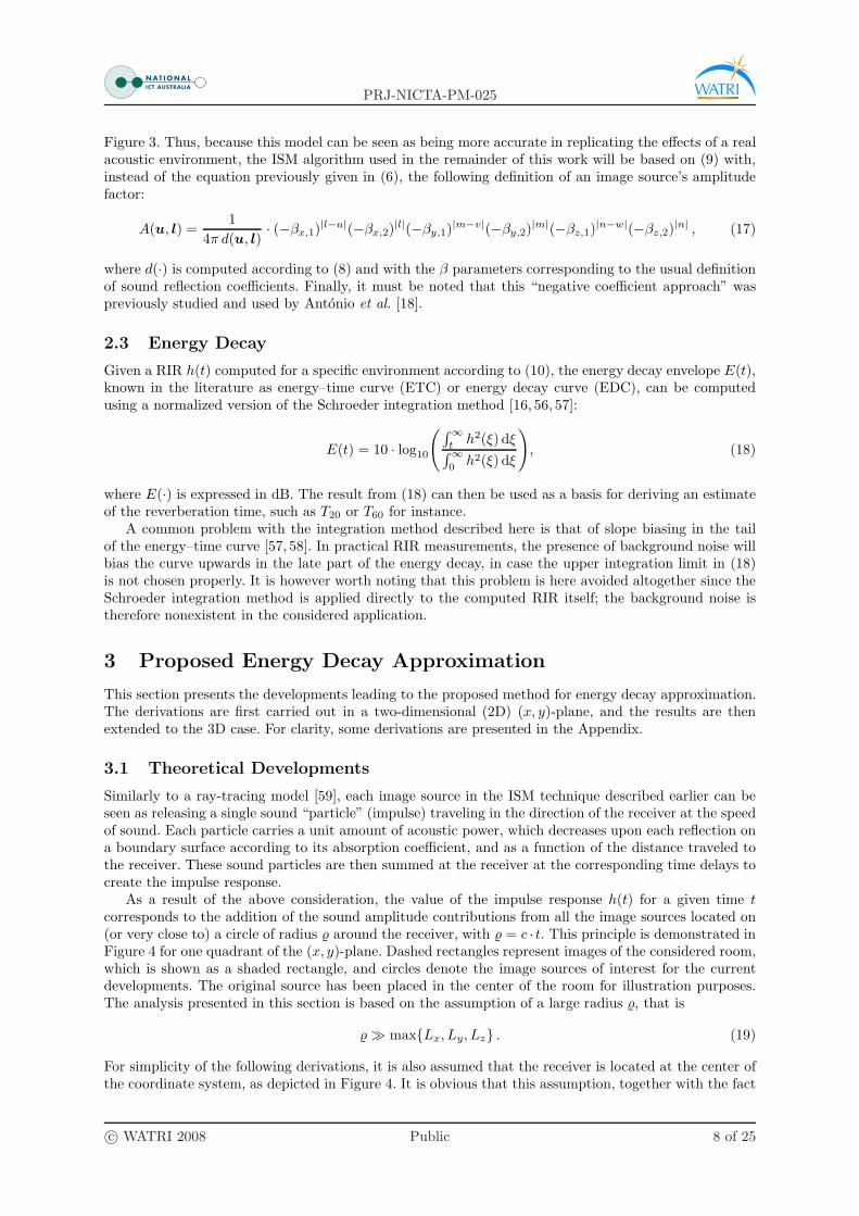
Similarly to a ray-tracing model [59], each image source in the ISM technique described earlier can beseen as releasing a single sound “particle” (impulse) traveling in the direction of the receiver at the speedof sound. Each particle carries a unit amount of acoustic power, which decreases upon each reflection ona boundary surface according to its absorption coefficient, and as a function of the distance traveled tothe receiver. These sound particles are then summed at the receiver at the corresponding time delays tocreate the impulse response.

As a result of the above consideration, the value of the impulse response h(t) for a given time tcorresponds to the addition of the sound amplitude contributions from all the image sources located on(or very close to) a circle of radius around the receiver, with = c · t. This principle is demonstrated inFigure 4 for one quadrant of the (x, y)-plane. Dashed rectangles represent images of the considered room,which is shown as a shaded rectangle, and circles denote the image sources of interest for the currentdevelopments. The original source has been placed in the center of the room for illustration purposes.The analysis presented in this section is based on the assumption of a large radius , that is

≫ max{Lx, Ly, Lz} . (19)

For simplicity of the following derivations, it is also assumed that the receiver is located at the center ofthe coordinate system, as depicted in Figure 4. It is obvious that this assumption, together with the fact


PRJ-NICTA-PM-025

βx,1

βx,1

βx,1

βx,2

βx,2

βy,1

βy,1

βy,2

βy,2

βy,2

x

y

ϑ

Lx

Ly

Figure 4: Two-dimensional representation of the ISM principle. Dashed lines represent the grid of imagesof the original room, which is displayed as a shaded rectangle. The β parameters indicate the reflectioncoefficients of the corresponding boundaries, and circles (◦) represent the considered image sources.

that some image sources do not lie perfectly on the considered circle, typically lead to approximationerrors that become negligible as the radius of the considered circle increases.

Let us now consider the i-th source located at an angle ϑi along the considered circle. Prior toreaching the receiver, its sound impulse traverses a number Wx , Wx(ϑi) of walls in the x-direction,and Wy , Wy(ϑi) walls in the y-direction, which can be determined in a straightforward manner on thebasis of the known position of the source. Consequently, the power contribution Pi(·) made by the i-thsource to the transfer function can be expressed as

Pi(, ϑi) =(β2

x,1)Wx2 (β2

x,2)Wx2 (β2

y,1)Wy

2 (β2y,2)

Wy

2

(4π)2. (20)

This expression makes use of the assumption that along the path to the receiver, the number of wallswith coefficient βx,1 (respectively βy,1) is approximately equal to the number of walls with coefficientβx,2 (respectively βy,2), that is, approximately equal to half the number of walls Wx/2 (respectivelyWy/2). This condition essentially becomes valid as the radius becomes large. Also, note that (20) usessquared-amplitude coefficients compared to (6) and (17), since the current developments are based onacoustic power rather than amplitude [11].

From this analysis, it follows that the value of the power impulse response hP (t) at time t, where thesubscript in hP (·) emphasizes the fact that the RIR is power-based, can be determined as

hP (t) =∑

i∈Ic

Pi(, ϑi) , (21)

with , (t) = c · t, and Ic representing the index set of the sources located on, or very close to theconsidered circle. The basis of the proposed approximation is then to consider (21) as a Riemann sumthat can be represented as the integral of a continuous function over the angle ϑ:

hP (t) · ∆ϑ =∑

i∈Ic

Pi(, ϑi) · ∆ϑ (22)

≈∫ 2π

0

P (, ϑ) dϑ . (23)


PRJ-NICTA-PM-025

With (20), the solution to this integral leads to an analytical expression, which can then be extendedto the 3D case. These derivations, which are provided in the Appendix, lead to the following estimatehP (·) ≈ hP (·) of the power transfer function:

hP (t) =1

8 r·

Bz

log(

By

Bx

) ·(

Ei1(log(

Bz

Bx

))+ log

(log(

Bz

Bx

))− Ei1

(log(

Bz

By

))− log

(log(

Bz

By

)))if Bx 6= By 6= Bz ,

Bz

log(

BzB

) ·(

Ei1(log(

Bz

B

))+ log

(log(

Bz

B

))+ γ

)if Bz = By 6= Bx , B or Bz = Bx 6= By , B ,

B−Bz

log(

BBz

) if Bz 6= Bx = By , B ,

B if Bx = By = Bz , B ,

(24)where , (t) = c · t as defined earlier, and with the following definitions:

Bx = (βx,1βx,2)/Lx , (25)

By = (βy,1βy,2)/Ly , (26)

Bz = (βz,1βz,2)/Lz , (27)

r =Lx + Ly + Lz

3, (28)

with γ = 0.5772157. . . the Euler–Mascheroni constant, and with Ein(ξ) denoting the exponential integral,defined in terms of the incomplete Gamma function for ξ 6= 0 as [60]

Ein(ξ) = ξn−1 · Γ(1 − n, ξ) . (29)

The exponential integral is a common mathematical function, implemented for instance as expint inMatlab, Ei in Maple, and ExpIntegralEi in Mathematica; alternatively, it can also be evaluatednumerically using a power series representation [60, 61].

An estimate of the energy decay curve can then be computed on the basis of (18) as

E(t) = 10 · log10

(∫∞

thP (ξ) dξ

∫∞

0hP (ξ) dξ

). (30)

In practice, the integrals on the right-hand side of (30) can be replaced with a Riemann sum as follows:

∫ ∞

t

hP (ξ) dξ ≈ T ·∞∑

i=0

hP (t+ iT ) . (31)

with an appropriate discretisation step T . As specified by fundamental principles of numerical integration,the validity of this approximation depends upon the function hP (·) being smooth and bounded in theconsidered interval, which is supported by the plots in Figure 5; it is also shown in the next section that(31) indeed holds true for the type of function defined in (24). Thus, the estimated energy–time curvecan be finally computed according to (30) and (31), and for t > t0, as

E(t) ≈ 10 · log10

( ∑∞i=0 hP (t+ iT )

∑∞i=0 hP (t0 + iT )

), t > t0. (32)

The introduction of the parameter t0 in (32) can be explained as follows. According to the assumptionsmade in this work, the EDC approximation is expected to be inaccurate for small values, that is, fort → 0. Therefore, the approximation formula in (32) can be considered as relevant only for values of tgreater than a specific threshold, denoted here as t0. Section 4.1 will provide more detail regarding anappropriate setting of the t0 parameter for numerical simulation purposes.

3.2 Discussion

Two distinct sources of error can be identified in relation to the expression proposed in (32). As mentionedabove, the assumption of a large radius will typically lead to a poor approximation of the true EDC as


PRJ-NICTA-PM-025

0 0.05 0.1 0.15 0.2 0.25 0.3 0.35

10−5

10−4

10−3

10−2

10−1

T20 ≈ 0.05sT20 ≈ 0.1sT20 ≈ 0.15sT20 ≈ 0.2s

time t (s)

hP(t

)

Figure 5: Numerical evaluation of the approximate power transfer function hP (·), for various levels ofreverberation, i.e., various β coefficients, in a room with dimensions r = [4.0m, 5.0m, 2.9m]T.

Figure 6 Figures 7 and 8r (m) [4.0, 5.0, 2.9]T [3.2, 4.0, 2.7]T

ps (m) [1.5, 1.0, 1.0]T [1.1, 1.0, 1.2]T

pr (m) [3.5, 3.8, 1.9]T [2.0, 3.0, 2.0]T

Fs (Hz) 16000 16000

Table 1: Environmental parameter setup for the results presented in Figures 6, 7 and 8.

t→ 0. In addition, the parameter t0 effectively introduces an additive error term ∆ in the denominatorof (32). This error term is related to the missing initial part of the denominator integration:

∆ , ∆(t0) =

∫ t0

0

h2(ξ) dξ , (33)

which is impossible to calculate on the basis of hP (·) due to the intrinsically poor approximation of

h2(·) provided by hP (·) for values of t below the threshold t0. The error term ∆ is however independentof the time variable t, and thus potentially creates a constant offset in the EDC approximation curveE(·). These two distinct effects (i.e., poor approximation at low values of t and offset due to ∆) will beillustrated more specifically in the following section.

Finally, the infinite sums in (32) have to be truncated to a finite set of indices in practice. As shown in

Figure 5, the function hP (ξ) tends towards 0 very quickly as ξ increases, and as a result, the summationcan be terminated relatively early while still providing a good approximation for practical purposes.

4 Experimental Results

4.1 Numerical Evaluations

This section provides some examples of the results obtained with the proposed approximation method.Figure 6 considers a typical enclosure setup, the details of which are provided in Table 1, for threedifferent levels of reverberation and assuming uniform reflection coefficients β for all enclosure surfaces.The solid lines represent the energy decay lines computed via (18) on the basis of the impulse responsessimulated with the ISM technique of Section 2.2. Circle markers (◦) indicate the values obtained via(24) and (32) computed at several discrete values of time. Figure 7 shows similar results, obtained usinga different room setup (see Table 1) in the case of non-uniform wall reflection coefficients, the valuesof which are given in Table 2. Note that the curves in Figure 7 correspond to a scenario where a pair


PRJ-NICTA-PM-025

0 0.1 0.2 0.3 0.4 0.5−70

−60

−50

−40

−30

−20

−10

0

(a) (b) (c)

time (s)

ED

C(d

B)

Figure 6: Examples of energy decay curves with uniform reflection coefficients. (a) β = 0.669 (T20 ≈0.05s), (b) β = 0.831 (T20 ≈ 0.1s), and (c) β = 0.889 (T20 ≈ 0.15s). Solid lines represent E(t) obtained

from ISM computations; circles (◦) indicate values obtained with the proposed approximation E(t).

Curve βx,1 βx,2 βy,1 βy,2 βz,1 βz,2

(a) T20 ≈ 0.05s 0.032 0.032 0.548 0.548 0.837 0.837(b) T20 ≈ 0.1s 0.675 0.675 0.787 0.787 0.915 0.915(c) T20 ≈ 0.15s 0.802 0.802 0.866 0.866 0.945 0.945

Table 2: Values of reflection coefficients for each boundary surface, for the curves displayed in Figure 7.

of opposing walls are significantly different in reflectivity compared to other surfaces; this specific casewas found to lead to discrepancies between estimated and measured reverberation time in Allen andBerkley’s original publication [1].

Despite several simplifying assumptions made in this work, Figures 6 and 7 demonstrate that theproposed EDC approximation technique is quite accurate when estimating the energy decay in RIRsproduced with the image source method. The overall decay rate, as well as the shape (curvature) of thedecay line for non-uniform β coefficients, matches the practical results relatively well. With respect tothe effects of the large-radius assumption mentioned previously, these numerical results clearly illustratethe discrepancy between the approximated and the practical results for low values of t, which appears asa slight upward bias at the beginning of the approximation curves. This effect becomes more pronouncedfor larger reverberation times, but remains nonetheless relatively negligible for practical purposes.

It must be noted here that the results in Figures 6 and 7 have been obtained with an optimal settingof the variable t0 (i.e., the time lag of the first value on the approximation curves). This effectivelycompensates for the constant error term mentioned in Section 3.2, and thus enables a better visualcomparison of the displayed results. In practice, a non-optimal setting of t0 would hence result in aslight offset in the corresponding EDC approximation curve. It was found empirically that choosingt0 = 1.5 · ‖ps − pr‖/c or t0 = 1.5 · r/c achieves a relatively good match for a large number of enclosuresizes and reflection coefficients. Note also that this offset only has a marginal effect when assessing theoverall energy decay of the considered RIR or when measuring quantities such as the reverberation time.If necessary, Ref. [62] further demonstrates the practical accuracy of the proposed method by means ofmore extensive numerical simulations. The development of a more accurate definition of the parametert0 is left as matter for further research, as a result of its minor impact on the considered analysis.

Finally, the different plots in Figure 8 provide an insight into the influence of the integration intervalT in (32). This figure displays the approximation results for three different integration lengths, computedwith T20 ≈ 0.1s and for an environmental setup as described in Table 1. These results clearly demonstratethe fact that the accuracy of the approximation remains very good regardless of the number of pointsconsidered along the curve, which corroborates the validity of the approximation in (31). If necessary, the


PRJ-NICTA-PM-025

0 0.1 0.2 0.3 0.4 0.5−70

−60

−50

−40

−30

−20

−10

0

(a) (b) (c)

time (s)

ED

C(d

B)

Figure 7: Examples of energy decay curves with non-uniform reflection coefficients, for (a) T20 ≈ 0.05s,(b) T20 ≈ 0.1s, and (c) T20 ≈ 0.15s. See Table 2 for corresponding β values. Solid lines represent E(t)

obtained from ISM computations; circles (◦) are values from the proposed approximation E(t).

computations can hence be made more efficient by reducing the number of points on the approximationcurve, with only a marginal reduction of the representation accuracy.

4.2 Discussion

The accuracy of the proposed EDC approximation method was tested and confirmed for a number ofscenarios considering different enclosure volumes, source and sensor positions, uniform and non-uniformreflection coefficients, and so forth. As shown in Section 4.1 and despite several simplifying assumptionsmade in Section 3.1, it is interesting to see that the discrepancy between the approximation and thepractical results remains relatively small even for very low radius values.

The proposed approximation technique hence enables designers to efficiently investigate the acousticalcharacteristics of a simulated room without the need to generate the RIRs of interest. Due to the consid-erable computational demands usually associated with the ISM technique, this consequently representsa substantial reduction of the resulting computation time during the analysis.

5 Application Example

This section describes a possible application of the developments presented in Section 3. It considersthe example of how to accurately determine the value of reflection coefficients in order to achieve agiven reverberation time in the considered virtual enclosure. As mentioned earlier, the image sourcemethod constitutes a major tool in the process of assessing the performance of many acoustic signalprocessing algorithms operating in reverberant environments. Typically, the image source model is usedto test the algorithms under consideration, in order to determine their robustness against increasinglevels of environmental reverberation. For the sake of a fair and consistent comparison, it is henceimportant to ensure that the algorithms are assessed using the same measure of reverberation across alltest simulations.

In recent literature [37, 42, 43, 46], a common approach to this assessment process involves the use ofthe well-known Sabine or Eyring formulae to determine reflection coefficients given a desired reverberationtime. The RIRs are then generated with the ISM technique (possibly using Peterson’s improvement [49]to Allen and Berkley’s original method [1]), and the performance results are finally displayed againstthe reverberation time that was used as a basis for the derivation of the β coefficients. As shown in thenext subsection, this approach is however subject to significant inaccuracies, especially for a non-uniformdefinition of the reflection coefficients in the considered room. This discrepancy between predicted and


PRJ-NICTA-PM-025

0 0.05 0.1 0.15 0.2 0.25 0.3 0.35

−60

−40

−20

0

0 0.05 0.1 0.15 0.2 0.25 0.3 0.35

−60

−40

−20

0

0 0.05 0.1 0.15 0.2 0.25 0.3 0.35

−60

−40

−20

0

(a)

(b)

(c)

time (s)

ED

C(d

B)

ED

C(d

B)

ED

C(d

B)

Figure 8: EDC approximation results with varying integration intervals, for T20 ≈ 0.1s and using thesame setup as in Figure 7. The integration interval is defined as (a) T = 0.014s, (b) T = 0.024s, and (c)T = 0.083s.

measured reverberation time was also observed in several publications of the acoustics literature [18, 63].As a result, it is very likely that the performance outcomes are ultimately presented for a reverberationlevel that does not correspond to the actual testing conditions.

An alternative approach chosen by various authors is to present the performance results versus thereflection coefficient itself [30–33,36]. However, contrary to more intuitive measures such as the rever-beration time T60 for instance, this way of presenting results does not provide any real insight into thepractical reverberation characteristics of the considered environment.

The EDC approximation method proposed in Section 3 can be used efficiently to alleviate theseproblems altogether, by providing an accurate and unequivocal correspondence between the reflectioncoefficients β and the resulting reverberation time.

5.1 Reverberation Time Prediction Formulae

Let us consider an enclosure with dimensions Lx × Ly × Lz where each boundary surface is assigned

an absorption coefficient as follows: αx,1 , α1, αx,2 , α2, αy,1 , α3, and so forth. For the sake ofsimplicity in the following presentation, it will be assumed that the coefficients are identical for each pairof opposing walls, i.e.,

α1 = α2 , α · wx , (34)

α3 = α4 , α · wy , (35)

α5 = α6 , α · wz , (36)

where wx, wy and wz are absorption weighting factors for the walls in the x, y and z dimensions, respec-tively. This representation allows for clearer derivations related to non-uniform absorption coefficients,which can be simply characterized in terms of the single parameter α used in conjunction with theweights vector w = [wx, wy, wz ] or, alternatively, the weighting ratio wx : wy : wz ≡ α1 : α3 : α5. It mustbe stressed however that this restriction is without loss of generality, since the following derivations canbe easily extended to the case where all coefficients have different values.


PRJ-NICTA-PM-025

As mentioned above, previous literature works have made an extensive use of well-known formulaeby Sabine or Eyring in order to determine the value of absorption coefficients achieving a desired rever-beration time T60. Many other formulae can also be found in the acoustics literature [64]. The presentwork will investigate several of these definitions, namely Sabine’s formula [65]:

T60,S(α,w) =0.161 · V∑6

i=1 Si αi

, (37)

Eyring’s formula [66]:

T60,E(α,w) =0.161 · V

−S · log(1 −∑6

i=1 Si αi/S) , (38)

Millington–Sette’s formula [67, 68]:

T60,MS(α,w) =0.161 · V

−∑6

i=1 Si · log(1 − αi), (39)

and Fitzroy’s formula [69]:

T60,F(α,w) =0.161 · V

S2·( −2LyLz

log(1 − (α1 + α2)/2

)− 2LxLz

log(1 − (α3 + α4)/2

)− 2LxLy

log(1 − (α5 + α6)/2

))

, (40)

where S is the total surface area of the enclosure, and Si, i = 1, . . . , 6, are the surface areas of eachindividual wall.

Given a specific weighting vector w, the problem of determining the value of α that achieves a desiredreverberation time, denoted here as T60,des, can be seen as a nonlinear optimization problem:

α(·) = arg minα∈[0,1]

∣∣T60,des − T60,(·)(α,w)∣∣ , (41)

where the subindex in α(·) indicates one of the formulae in (37)–(40). This minimization problem canbe solved numerically using, for instance, a golden section search algorithm with parabolic interpolation[70], as implemented by the function fminbnd in Matlab.

In the following, the reverberation time will be characterized using T20 rather than T60, where T20 ishere defined according to the classical formula as the time required by the RIR energy E(·), defined by(18), to decay from −5dB to −25dB:

T20 = E−1(−25) − E−1(−5) , (42)

where E−1(·) represents the inverse of the EDC function E(·), i.e., E−1(ξ) corresponds to the time lag tξfor which E(tξ) = ξ. The reason for using T20 instead of T60 is solely in order to reduce the computationalload when measuring the reverberation time in simulated RIRs in Section 5.3. As a result of using non-uniform absorption coefficients, the EDC will typically display a non-negligible curvature, which in turnmeans that it would be inaccurate to measure T60 by interpolation of the initial decay slope in theenergy–time curve. By using the parameter T20 instead of T60, it is hence only necessary to compute theEDC down to −25dB (or slightly below), which involves significantly less image sources during the RIRcomputations. It is however emphasized once more that this substitution is only to facilitate the displayof the comparison results; the present developments are valid for any quantity of interest defined on thebasis of the EDC, such as T60, T30, early decay time, etc.

Because the various classical formulae given in (37)–(40) have been derived on the basis of the averagesound absorption within the room, or assuming a homogenous spatial distribution of the sound power(diffuse field), they implicitly assume a linear energy decay in the resulting EDC. It follows that for thesecases, the T20 value is simply defined as

T20,(·)(α,w) = T60,(·)(α,w)/3 . (43)


PRJ-NICTA-PM-025

0 0.05 0.1 0.15 0.2 0.25 0.3 0.35

−50

−40

−30

−20

−10

0

T20,EDC

time (s)

ED

C(d

B)

Figure 9: Determining the reverberation time T20 from the proposed EDC approximation results.

5.2 Reverberation Time Prediction using EDC Approximation

The EDC approximation method described in Section 3 can be used in a straightforward manner inorder to determine the value of the absorption coefficients αi achieving a desired reverberation time.As depicted in Figure 9, the numerical value of T20,EDC(α,w) for a given absorption parameter α andweighting vector w is obtained by simply computing the EDC approximation curve according to (24) and(32), and determining the corresponding reverberation time directly from it. A first-order interpolationbetween points is also used in this process to refine the estimate. Using this approach, the α parametervalue that yields the desired reverberation time T20,des is finally obtained as the solution to the sameoptimization problem as given previously in (41).

5.3 Numerical Results

In this section, the accuracy of the proposed EDC approximation method is assessed and compared tothe currently established formulae using the following test. Given a specific target reverberation timeT20,des and weight vector w, the absorption parameter α is determined via (41) for each of the consideredreverberation time approximation formulae in (37)–(40), as well as the proposed technique as describedin Section 5.2. The image source method is then used with the resulting α values to generate a number ofRIRs in the considered environment, and the “true” reverberation time value T20,meas is then measureddirectly from the RIR using the definition in (42). For the proposed EDC approximation method, thefrequency-domain ISM algorithm with negative reflection coefficients is used to simulate the RIRs, asdescribed in Section 2.2. The original implementation of Allen and Berkley (positive reflection coefficients)is used in conjunction with the classical reverberation prediction methods, since this represents theapproach that is currently widely used in the literature. The resulting error ε is then simply defined, foreach method, as

ε =∣∣T20,des − T20,meas

∣∣ . (44)

For a given T20,des, this process is repeated for a total of 30 randomly selected source and receiverpositions, in each of eight different rooms, ranging from a size of 2.7m× 3m× 2.5m (volume of 20.25m3)to 6.53m × 7.26m × 4.27m (volume of 202.5m3). Finally, Figure 10 presents the distribution of theresulting 240 error values obtained with each method under consideration and for each desired value ofreverberation time, in the form of a median and interquartile-range plot. Each plot in this figure presentsthe results obtained with a different ratio of absorption coefficient wx : wy : wz , which represent variouslevels of non-uniformity amongst the specific absorption coefficients, including the special case of equalcoefficient values.

Note that these graphs only display results for simulation conditions that are considered to be “phys-ically” attainable: assuming non-uniform wall coefficients results in some surfaces having non-total ab-sorption (i.e., α 6= 1), which in turn will generate a minimum, non-vanishing amount of reverberation inthe enclosure. In other words, some values of T20 below a certain limit will be impossible to generate givena specific room r and non-uniform weighting vector w. Error results below this limit are not displayedin Figure 10, since it is known that such simulation conditions will yield large errors by definition.


PRJ-NICTA-PM-025

0.05 0.1 0.15 0.2 0.250

0.02

0.04

0.06

0.08

0.1

0.12

Fitzroy

Eyring

Millington−Sette

Sabine

Proposed method (a)

T20,des (s)

erro

rε

(s)

0.05 0.1 0.15 0.2 0.250

0.02

0.04

0.06

0.08

0.1

0.12

Fitzroy

Eyring

Millington−Sette

Sabine

Proposed method (b)

T20,des (s)

erro

rε

(s)

0.05 0.1 0.15 0.2 0.250

0.02

0.04

0.06

0.08

0.1

0.12

0.14

0.16

0.18

Fitzroy

Eyring

Millington−Sette

Sabine

Proposed method (c)

T20,des (s)

erro

rε

(s)

0.05 0.1 0.15 0.2 0.250

0.05

0.1

0.15

0.2

0.25

0.3

0.35

0.4

0.45

0.5

Fitzroy

Eyring

Millington−Sette

Sabine

Proposed method (d)

T20,des (s)

erro

rε

(s)

Figure 10: Distribution of the resulting T20 prediction error, for each considered method: error barsrepresent the interquartile range (25-th and 75-th percentile, respectively), whereas center markers cor-respond to the median of the distribution. The absorption coefficient ratio wx : wy : wz is defined as (a)1.0 : 1.0 : 1.0, (b) 1.0 : 0.8 : 0.6, (c) 1.0 : 0.6 : 0.3, and (d) 1.0 : 0.5 : 0.1.

5.4 Discussion

Figure 10 shows that the proposed EDC approximation method is able to maintain a low level of errorfor the considered test scenarios, and provides the best results among the five considered T20 predictionmethods. While most of the other methods display a large resulting error, some of them also have awidely spread distribution of their error values (large interquartile range). This results from the fact thatthe accuracy of such methods varies significantly as a function of the considered room size: typically, suchmethods will generate larger errors as the size of the considered enclosure becomes smaller. On the otherhand, the technique proposed in this paper is able to maintain a relatively concentrated distributionthroughout the simulations, which highlights the fact that it provides good results for a wide range ofroom volumes.

When considering the various formulae described in Section 5.1, it can be seen on the basis of Figure 10that none of them provides a consistently low level of estimation error. On the contrary, for most of themthe error becomes larger as the desired value of reverberation time increases. This consequently raisessome doubts regarding their usefulness in predicting the reverberation level in simulated RIRs, whichcan be regarded as being of some concern since several publications have been published which provideassessment results based on these formulae [42, 43, 45–47]. On the other hand, the results obtained withthe proposed EDC approximation are consistently better than any other method. For the proposed tech-nique, the largest error in fact occurs in the case of uniform absorption coefficients and large T20 values,as shown in the top left-hand graph of Figure 10. This is a direct result of the upwards biasing problem


PRJ-NICTA-PM-025

of the EDC approximation curve, as observed in Section 4.1, and which becomes more pronounced whenthe “true” EDC is close to a straight line, i.e., in the case of uniform α coefficients. Finally, it is alsointeresting to notice how Fitzroy’s formula becomes more accurate as the level of non-uniformity in theabsorption coefficients increases. This formula was empirically derived to account for a non-uniform defi-nition of the absorption coefficients in the room [69], which explains this effect in the results of Figure 10.

In summary, the results displayed in Figure 10 demonstrate that the proposed EDC approximationmethod can be used as an efficient tool in the process of analyzing acoustic signal processing algorithms,evaluated on the basis of image source simulations. The results in this section show that the accuracyof this approximation technique allows to generate simulated RIRs with a reverberation time within asmall percentage of the desired T20 value. Consequently, this approach can be efficiently implemented inreplacement of the only current solution to this specific issue, i.e., a lengthy trial-and-error process usingtime-consuming ISM simulations.

6 Conclusion

This paper proposes a new method for approximating the energy decay in simulated room impulse re-sponses. It was demonstrated that the proposed technique provides an accurate approximation of thepower transfer function generated on the basis of a modified version of the widely-used image sourcemodel: this modification involves computations in the frequency domain to account for non-integertime delays, and implements a phase inversion upon each reflection of the sound rays off the enclo-sure boundaries. As a result, the simulated transfer functions look more natural and constitute a betterrepresentation of practical impulse response measurements, compared to Allen and Berkley’s originalmethod.

This paper also considered an application example where the proposed approximation method isproving useful, namely when implemented during the testing phase of single or multi-channel acousticsignal processing algorithms. Using the approach described in this work, it is possible to accuratelydetermine the value of absorption coefficients required to achieve a desired reverberation level in theenvironment, which results in two valuable benefits. Since this process can now be carried out withoutthe need for time-consuming image method simulations, the time required for the design or analysis ofalgorithms using the image source method is drastically reduced. Also, it ensures that the algorithms aretested, and performance results are presented, versus a reverberation level that corresponds more or lessexactly to what was used during the algorithm simulations. This ensures uniformity of the results whencomparing the algorithm performance presented by various authors in different publications.

Finally, the technique described in this work can also be of potential interest in other fields of acous-tic design and engineering, such as, for instance, virtual auditory environments, perceptual acoustics,interactive architectural acoustics, reverberant sound field modeling, etc.

Acknowledgments

This work was supported by National ICT Australia (NICTA). NICTA is funded through the AustralianGovernment’s Backing Australia’s Ability initiative, in part through the Australian Research Council.


PRJ-NICTA-PM-025

Appendix

This Appendix contains the derivations leading to the result of (24), starting from a two-dimensionalconsideration of the problem (see Figure 4). From (20), the contribution to the power RIR from an imagesource, located at angle ϑ on a circle with radius , is

P (, ϑ) =(βx,1βx,2)

Wx(βy,1βy,2)Wy

(4π)2, (45)

with , (t) = c · t. On the basis of Figure 4, and using a first-order approximation, the number ofboundary surfaces between the source and the receiver, in the x and y dimensions, are defined as follows(for ϑ ∈ [0, π/2]):

Wx =

Lx·(1 − 2ϑ

π

), (46)

Wy =

Ly· 2ϑ

π. (47)

From (23), the estimated power transfer function hP (·) results as follows:

hP (t) ≈ hP (t) =4

∆ϑ

∫ π2

0

P (, ϑ) dϑ , (48)

where the analysis has been restricted to a quarter of the circle, for ϑ ∈ [0, π/2], as a result of thesymmetry in the problem definition. The angular variable ∆ϑ can be determined as

∆ϑ =2π

Ns, (49)

where Ns corresponds to the total number of image sources considered on the circle (or located veryclose to it). From Figure 4, it can be seen that for ϑ→ 0, the average distance between the image sourceson the circle approaches Ly; similarly, for ϑ → π/2, it approaches Lx. Consequently, the parameter Ns

is here defined as the circle’s circumference divided by the average room dimension, i.e.,

Ns =2π

r, (50)

with r = (Lx + Ly)/2. The value of ∆ϑ then follows as ∆ϑ = r/, which leads to the final power RIRapproximation for the 2D setting:

hP (t) =4

r

∫ π2

0

P (, ϑ) dϑ . (51)

In effect, the various approximations used in the developments so far take into account the averagedistribution of the image sources located in the vicinity of the considered circle, rather than only thosesources located exactly at a radius from the receiver.

The extension of the above derivations to the 3D case is based on the same approach, as illustrated inFigure 11. The total power in the RIR for a given time lag t corresponds to the sum of the contributionsfrom image sources located on, or very close to a sphere with corresponding radius = c · t, centeredon the origin. With the introduction of the polar angle ϕ ∈ [0, π] (see Figure 11), the correspondingRiemann sum then follows as

∑

i∈Is

Pi(, ϑi, ϕi) · ∆ϑ∆ϕ =

∫ π

0

∫ 2π

0

P (, ϑ, ϕ) dϑ dϕ , (52)

where Is represents the index set of the sources located on the sphere. The main issue with (52) isregarding the computation of the term ∆ϑ∆ϕ. As demonstrated in Figure 11, simply defining uniformlyspaced points in ϑ and ϕ (as done in the 2D derivations), leads to a grid on the sphere that obviously doesnot correspond to the distribution of image sources in the ISM technique. The “true” distribution of the


PRJ-NICTA-PM-025

x

y

z

ϑ

ϕ

Figure 11: Definition of variables in a spherical coordinate system. The grid of points on the sphere isnot representative of the 3D distribution of image sources in the ISM technique.

sources corresponds to a nonlinear spherical grid, which is quite complex to derive mathematically fromthe grid of mirror rooms defined by the image source method. One possible approach for a 3D scenario isto update the expression for the 2D case obtained in (51); this approximation has been empirically foundto be sufficiently accurate, due mainly to the normalization process carried out in (30) when computingthe energy decay values. Again limiting the analysis to one eighth of the sphere, (51) becomes

hP (t) =8

r

∫ π2

0

∫ π2

0

P (, ϑ, ϕ) dϑ dϕ , (53)

where r now includes the room dimension for the z coordinate:

r =Lx + Ly + Lz

3, (54)

and with the 3D extension of the power amplitude coefficient and number of walls:

P (, ϑ, ϕ) =(βx,1βx,2)

Wx(βy,1βy,2)Wy (βz,1βz,2)

Wz

(4π)2, (55)

Wx =

Lx·(1 − 2ϑ

π

)· 2ϕ

π, (56)

Wy =

Ly· 2ϑ

π· 2ϕ

π, (57)

Wz =

Lz·(1 − 2ϕ

π

). (58)

Inserting (55)–(58) into (53) and analytically solving the double integral finally leads to the result in(24). As shown in this equation, the resulting expression can be simplified further in case equality holdsbetween the value of certain parameters.

In Equation (24), rotation of the coordinates x, y and z can be applied in order to avoid cases thatwould otherwise lead to negative arguments for the exponential integral Ei1(·) or for the logarithm func-tion. For instance, if a given environmental setup leads to Bz = Bx 6= By with By > Bz, Equation (24)involves the logarithm of a negative argument, which in turn generates complex values for the powertransfer function. Such a case can be dealt with by swapping the coordinates y and z, i.e., by carrying


PRJ-NICTA-PM-025

out the computations with the newly defined variables B′y , Bz and B′

z , By. As a result, this leads to acase where B′

z 6= B′y = Bx, which can be successfully handled by Equation (24). This type of coordinate

rotation effectively corresponds to a simple re-definition of the axis coordinates (here, e.g., y′ , z andz′ , y) with respect to the spherical coordinate system shown in Figure 11, and does not change thegenerality or validity of the main result provided in (24).


PRJ-NICTA-PM-025

References

[1] J. Allen and D. Berkley. Image method for efficiently simulating small-room acoustics. Journal ofthe Acoustical Society of America, 65(4):943–950, April 1979.

[2] J. Borish. Extension of the image model to arbitrary polyhedra. Journal of the Acoustical Societyof America, 75(6):1827–1836, June 1984.

[3] H. Lee and B.-H. Lee. An efficient algorithm for the image model technique. Applied Acoustics,24(2):87–115, 1988.

[4] U. Kristiansen, A. Krokstad, and T. Follestad. Extending the image method to higher-order reflec-tions. Applied Acoustics, 38(2–4):195–206, 1993.

[5] M. Vorlander. Simulation of the transient and steady-state sound propagation in rooms using anew combined ray-tracing/image-source algorithm. Journal of the Acoustical Society of America,86(1):172–178, July 1989.

[6] S. Dance, J. Roberts, and B. Shield. Computer prediction of sound distribution in enclosed spacesusing an interference pressure model. Applied Acoustics, 44(1):53–65, 1995.

[7] M. Hodgson. On the accuracy of models for predicting sound propagation in fitted rooms. Journalof the Acoustical Society of America, 88(2):871–878, August 1990.

[8] B. Gibbs and D. Jones. A simple image method for calculating the distribution of sound pressurelevels within an enclosure. Acustica, 26:24–32, 1972.

[9] Y. Lam. Issues for computer modelling of room acoustics in non-concert hall settings. AcousticalScience and Technology, 26(2):145–155, 2005.

[10] M. Kleiner, R. Orlowski, and J. Kirszenstein. A comparison between results from a physical scalemodel and a computer image source model for architectural acoustics. Applied Acoustics, 38(2–4):245–265, 1993.

[11] J. Suh and P. Nelson. Measurement of transient response of rooms and comparison with geometricalacoustic models. Journal of the Acoustical Society of America, 105(4):2304–2317, April 1999.

[12] K. Li and K. Iu. Propagation of sound in long enclosures. Journal of the Acoustical Society ofAmerica, 116(5):2759–2770, November 2004.

[13] K. Li and K. Iu. Full-scale measurements for noise transmission in tunnels. Journal of the AcousticalSociety of America, 117(3):1138–1145, March 2005.

[14] K. Iu and K. Li. The propagation of sound in narrow street canyons. Journal of the AcousticalSociety of America, 112(2):537–550, August 2002.

[15] S. Dance and B. Shield. The complete image-source method for the prediction of sound distributionin non-diffuse enclosed spaces. Journal of Sound and Vibration, 201(4):473–489, 1997.

[16] K. Li and P. Lam. Prediction of reverberation time and speech transmission index in long enclosures.Journal of the Acoustical Society of America, 117(6):3716–3726, June 2005.

[17] J. Kang. A method for predicting acoustic indices in long enclosures. Applied Acoustics, 51(2):169–180, June 1997.

[18] J. Antonio, L. Godinho, and A. Tadeu. Reverberation times obtained using a numerical modelversus those given by simplified formulas and measurements. Acta Acustica united with Acustica,88(2):252–261, March/April 2002.

[19] J. Rindel and C. Lynge Christensen. Room acoustic simulation and auralization—How close can weget to the real room? In Proceedings of the Eighth Western Pacific Acoustics Conference, Melbourne,Australia, April 2003. Keynote lecture, 8 pages.


PRJ-NICTA-PM-025

[20] H. Lehnert and J. Blauert. Virtual auditory environment. In Proceedings of the IEEE InternationalConference on Advanced Robotics, volume 1, pages 211–216, Pisa, Italy, June 1991.

[21] H. Møller. Fundamentals of binaural technology. Applied Acoustics, 36(3–4):171–218, 1992.

[22] L. Savioja, T. Lokki, and J. Huopaniemi. Auralization applying the parametric room acousticmodeling technique—the DIVA auralization system. In Proceedings of the International Conferenceon Auditory Display, pages 219–224, Kyoto, Japan, July 2002.

[23] T. Lokki, L. Savioja, R. Vaananen, J. Huopaniemi, and T. Takala. Creating interactive virtualauditory environments. IEEE Computer Graphics and Applications, 22(4):49–57, July 2002.

[24] N. Tsingos and J.-D. Gascuel. Soundtracks for computer animation: sound rendering in dynamicenvironments with occlusions. In Proceedings of the Graphics Interface Conference, pages 9–16,Kelowna, BC, Canada, May 1997.

[25] J. Miller and E. Wenzel. Recent developments in SLAB: a software-based system for interactivespatial sound synthesis. In Proceedings of the Eighth International Conference on Auditory Display,pages 403–408, Kyoto, Japan, July 2002.

[26] T. Lentz, D. Schroder, M. Vorlander, and I. Assenmacher. Virtual reality system with integratedsound field simulation and reproduction. EURASIP Journal on Advances in Signal Processing, 2007,2007. Article ID 70540, 19 pages.

[27] E. Wenzel, J. Miller, and J. Abel. A software-based system for interactive spatial sound synthesis.In Proceedings of the International Conference on Auditory Display, pages 151–156, Atlanta, GA,USA, April 2000.

[28] J.-M. Jot. Real-time spatial processing of sounds for music, multimedia and interactive human-computer interfaces. Multimedia Systems, 7(1):55–69, 1999.

[29] D. Zotkin, R. Duraiswami, and L. Davis. Rendering localized spatial audio in a virtual auditoryspace. IEEE Transactions on Multimedia, 6(4):553–564, August 2004.

[30] M. Ikram and D. Morgan. A multiresolution approach to blind separation of speech signals in areverberant environment. In Proceedings of the IEEE International Conference on Acoustics, Speech,and Signal Processing, volume 5, pages 2757–2760, Salt Lake City, UT, USA, May 2001.

[31] M. Ikram and D. Morgan. A beamforming approach to permutation alignment for multichannelfrequency-domain blind speech separation. In Proceedings of the IEEE International Conference onAcoustics, Speech, and Signal Processing, volume 1, pages 881–884, Orlando, FL, USA, May 2002.

[32] J. Hopgood, P. Rayner, and P. Yuen. The effect of sensor placement in blind source separation. InProceedings of the IEEE Workshop on the Applications of Signal Processing to Audio and Acoustics,pages 95–98, New Paltz, NY, USA, October 2001.

[33] B. Radlovic, R. Williamson, and R. Kennedy. Equalization in an acoustic reverberant environment:robustness results. IEEE Transactions on Speech and Audio Processing, 8(3):311–319, May 2000.

[34] F. Talantzis and D. Ward. Robustness of multichannel equalization in an acoustic reverberantenvironment. Journal of the Acoustical Society of America, 114(2):833–841, August 2003.

[35] D. Ward. On the performance of acoustic crosstalk cancellation in a reverberant environment.Journal of the Acoustical Society of America, 110(2):1195–1198, August 2001.

[36] Y. Huang and J. Benesty. A class of frequency-domain adaptive approaches to blind multichannelidentification. IEEE Transactions on Signal Processing, 51(1):11–24, January 2003.

[37] E. Lehmann and A. Johansson. Particle filter with integrated voice activity detection for acousticsource tracking. EURASIP Journal on Advances in Signal Processing, 2007, 2007. Article ID 50870,11 pages.


PRJ-NICTA-PM-025

[38] D. Ward, E. Lehmann, and R. Williamson. Particle filtering algorithms for tracking an acousticsource in a reverberant environment. IEEE Transactions on Speech and Audio Processing, 11(6):826–836, November 2003.

[39] J. Vermaak and A. Blake. Nonlinear filtering for speaker tracking in noisy and reverberant envi-ronments. In Proceedings of the IEEE International Conference on Acoustics, Speech, and SignalProcessing, volume 5, pages 3021–3024, Salt Lake City, UT, USA, may 2001.

[40] K. Palomaki, G. Brown, and J. Barker. Missing data speech recognition in reverberant conditions.In Proceedings of the IEEE International Conference on Acoustics, Speech, and Signal Processing,volume 1, pages 65–68, Orlando, FL, USA, May 2002.

[41] K. Palomaki, G. Brown, and D. Wang. A binaural processor for missing data speech recognition inthe presence of noise and small-room reverberation. Speech Communication, 43(4):361–378, 2004.

[42] S. Doclo and M. Moonen. GSVD-based optimal filtering for single and multimicrophone speechenhancement. IEEE Transactions on Signal Processing, 50(9):2230–2244, September 2002.

[43] P. Aarabi and G. Shi. Phase-based dual-microphone robust speech enhancement. IEEE Transactionson Systems, Man, and Cybernetics—Part B: Cybernetics, 34(4):1763–1773, August 2004.

[44] J. Chen, J. Benesty, and Y. Huang. Robust time delay estimation exploiting redundancy among mul-tiple microphones. IEEE Transactions on Speech and Audio Processing, 11(6):549–557, November2003.

[45] P. Aarabi. Self-localizing dynamic microphone arrays. IEEE Transactions on Systems, Man, andCybernetics—Part C: Applications and Reviews, 32(4):474–484, November 2002.

[46] M. Brandstein and H. Silverman. A robust method for speech signal time-delay estimation inreverberant rooms. In Proceedings of the IEEE International Conference on Acoustics, Speech, andSignal Processing, volume 1, pages 375–378, Munich, Germany, April 1997.

[47] S. Doclo and M. Moonen. Robust adaptive time delay estimation for speaker localization in noisy andreverberant acoustic environments. EURASIP Journal on Applied Signal Processing, 2003(11):1110–1124, 2003.

[48] Y. Zheng, R. Goubran, and M. El-Tanany. Robust near-field adaptive beamforming with distancediscrimination. IEEE Transactions on Speech and Audio Processing, 12(5):478–488, September 2004.

[49] P. Peterson. Simulating the response of multiple microphones to a single acoustic source in areverberant room. Journal of the Acoustical Society of America, 80(5):1527–1529, November 1986.

[50] H. Kuttruff. Room acoustics. Spon Press, London – New York, Fourth edition, August 2000.

[51] C. Nocke. In-situ acoustic impedance measurement using a free-field transfer function method.Applied Acoustics, 59(3):253–264, March 2000.

[52] M. Delany and E. Bazley. Acoustical properties of fibrous absorbent materials. Applied Acoustics,3(2):105–116, April 1970.

[53] B. Brouard, D. Lafarge, J.-F. Allard, and M. Tamura. Measurement and prediction of the reflec-tion coefficient of porous layers at oblique incidence and for inhomogeneous waves. Journal of theAcoustical Society of America, 99(1):100–107, January 1996.

[54] M. Schroeder. Integrated-impulse method measuring sound decay without using impulses. Journalof the Acoustical Society of America, 66(2):497–500, August 1979.

[55] B. Katz. International round robin on room acoustical impulse response analysis software 2004.Acoustics Research Letters Online, 5(4):158–164, October 2004.

[56] M. Schroeder. New method of measuring reverberation time. Journal of the Acoustical Society ofAmerica, 37(6):409–412, June 1965.


PRJ-NICTA-PM-025

[57] M. Karjalainen, P. Antsalo, A. Makivirta, T. Peltonen, and V. Valimaki. Estimation of modaldecay parameters from noisy response measurements. Journal of the Audio Engineering Society,50(11):867–878, November 2002.

[58] D. Morgan. A parametric error analysis of the backward integration method for reverberation timeestimation. Journal of the Acoustical Society of America, 101(5):2686–2693, May 1997.

[59] A. Krokstad, S. Strøm, and S. Sørsdal. Calculating the acoustical room response by use of a raytracing technique. Journal of Sound and Vibration, 8(1):118–125, 1968.

[60] M. Abramowitz and I. Stegun. Handbook of mathematical functions with formulas, graphs, andmathematical tables. Dover Publications, New York, 1965.

[61] W. Press, B. Flannery, S. Teukolsky, and W. Vetterling. Numerical recipes in C: the art of scientificcomputing. Cambridge University Press, Cambridge, Second edition, 1992.

[62] E. Lehmann, A. Johansson, and S. Nordholm. Reverberation-time prediction method for roomimpulse responses simulated with the image-source model. In Proceedings of the IEEE Workshopon Applications of Signal Processing to Audio and Acoustics (WASPAA’07), pages 159–162, NewPaltz, NY, USA, October 2007.

[63] S. Dance and B. Shield. Modelling of sound fields in enclosed spaces with absorbent room surfaces—Part II: absorptive panels. Applied Acoustics, 61(4):373–384, December 2000.

[64] R. Neubauer and B. Kostek. Prediction of the reverberation time in rectangular rooms with non-uniformly distributed sound absorption. Archives of Acoustics, 26(3):183–202, 2001.

[65] W. Sabine. Collected papers on acoustics. Dover Publications, New York, 1964.

[66] C. Eyring. Reverberation time in “dead” rooms. Journal of the Acoustical Society of America,1(2A):217–241, January 1930.

[67] W. Sette. A new reverberation time formula. Journal of the Acoustical Society of America, 4(3):193–210, January 1933.

[68] G. Millington. A modified formula for reverberation. Journal of the Acoustical Society of America,4(1A):69–82, July 1932.

[69] D. Fitzroy. Reverberation formula which seems to be more accurate with nonuniform distributionof absorption. Journal of the Acoustical Society of America, 31(7):893–897, July 1959.

[70] R. Brent. Algorithms for minimization without derivatives. Prentice-Hall, Englewood Cliffs, NJ,1973.


scientiﬁc report [email protected] - eric a. lehmann · scientiﬁc report document reference: ......

Documents